informality, corruption, and inequality...1 informality, corruption, and inequality 1 introduction...
TRANSCRIPT
Informality, Corruption, and Inequality*
(Preliminary, October 2011)
Ajit Mishraa Ranjan Rayb
University of Bath, UK Monash University, Australia
Abstract
The paper looks at the determinants of the size of the informal sector. We argue that corruption and informality complement each other and are jointly determined by various market and non-market variables. Our theoretical model and the empirical exercises focus on wealth/income inequality as a key determinant of informality and corruption, with a high degree of inequality leading to a bigger informal sector. We discuss various channels through which inequality can impact the size of the informal sector. JEL Classification Codes: O15; O17; K4. Keywords: Informal Sector; Shadow economy; Corruption; Inequality; Credit Market
*We have benefited from discussions with Dilip Mookherjee, Jihyun Kim, Indranil Dutta and seminar participants at Monash, Bath, and Warwick. We would like to thank Ishita Chatterjee for invaluable research assistance. Part of the work was done while Ajit Mishra was visiting Monash University. Financial support and hospitality for his visit are gratefully acknowledged. a Department of Economics, University of Bath, Bath, UK, BA2 7AY Email: [email protected]; corresponding author. b Department of Economics, Monash University, Clayton,Victoria,3800, Australia. Email: [email protected]
1
Informality, Corruption, and Inequality
1 Introduction The “informal sector”, which has also been referred to as the “shadow or
underground economy” [Schneider and Enste (2000)], and “unofficial activity”
[Friedman, et. al. (2000)], plays a significant role in developing economies. The
precise definition of the informal sector varies considerably but it generally refers to
economic activity that is neither taxed nor monitored by a government.1 It is clear
that the existence of this sector poses serious challenges to policy makers in
developing countries. First, it is a significant source of revenue leaks for the
government that deprives the economy of budgetary resources. Second, since its
activities are hidden from public scrutiny, it is not subject to labour standards such as
minimum wages, decent and non hazardous working conditions, child labour laws,
etc. Third, in denying access to official credit channels, firms operating informally are
denied access to modern technology leading to loss of productivity. Last, the informal
sector provides gainful employment to large sections of the workforce though the
informal labor does not enjoy the various social security benefits of the formal
counterpart.
There have been several interesting attempts to measure the size of the informal
economy and examine some of the factors that explain the existence and size of the
informal sector.2 While by the very nature of the concept of informality, all such
measures must be tentative, the available evidence suggests that the size of the
informal sector is quite significant. Informal sector exists in all economies in varied
sizes, but its size and determinants are of particular interest in the context of
developing economies.
This paper examines two aspects of the informal sector that have not featured much in
the literature, namely, the interaction of the informal sector with corruption, and the
role that rising income inequality plays in supporting the informal sector. This paper
1 In many definitions the shadowy nature of this sector is not raised at all. For example, the Report on Definitional and Statistical Issues relating Informal Economy (Government of India) recommends that the informal sector be defined to consist of all unincorporated private enterprises owned by individuals or households …., with less than ten total workers. In this paper, the focus is more on the illegal shadowy side of the informal sector. This is partly because the actual data used in the paper identifies informality with ‘percentage of undeclared sales’. 2 See Straub (2005), Dabla-Norris et al (2008), Choi and Thum (2005), Johnson et al (2000 ), Friedman et al (2000), Schneider and Enste (2000) among others.
2
develops analytical arguments that suggest that there is complementarity between the
informal economy and corruption and that higher inequality leads to larger informal
sector. We also provide support for the theoretical arguments with empirical evidence
based on a large cross country survey data containing firms’ responses.
Corruption entails social and economic costs to development that are similar to those
of informality. The magnitude of corruption is also believed to be comparable to that
of the informal sector.3 It is worth pointing out that factors such as “the rise of the
burden of taxes…declining tax morale” identified by Schneider and Enste (2000) or
the lack of a quality legal system identified by Dabla-Norris, et. al. (2008) as possible
explanations for the informal sector also figure prominently as likely explanations for
corruption. Some of the earlier studies on the informal sector [Johnson et. al. (1998),
Friedman et. al. (2000), Djankov et. al.(2002)] have noted the possible link between
corruption and informality. For example, Djankov et. al. (2002) suggests that
“countries with heavier regulation of entry have higher corruption and larger
unofficial economies”. Our paper contributes to this literature by developing a model
of the joint determination of corruption and informality, something lacking in the
existing literature. 4 From a policy viewpoint, this is an important issue to investigate
since if, as this paper shows, the interaction between the two is mutual, positive and
significant, with informality and corruption feeding off one another, then an integrated
strategy in dealing with both is likely to be more effective.
The issue of increasing inequality possibly leading to rising informal sector is also
significant in the present context.5 Rosser et.al. (2000), Chong and Gradstein (2007)
report a positive relationship between inequality and informality. Our paper is perhaps
closer to Chong and Gradstein (2007) but the analytical framework and the data sets
are quite different. Our paper explores the precise mechanism(s) through which
inequality affects the informal sector and we find strong evidence for the positive
relationship in a large sample of firms across several countries. In this context our
mechanism is very similar to the credit market channel discussed by Straub (2005).
Straub (2005) argues that lack of access to formal credit encourages firms to go
informal. The inequality variable adds to this explanation since in a more unequal
3 See Mishra (2005) for a comprehensive survey and for some of the important contributions in the corruption literature. 4 Recently we came across Samuel and Alger (2011) which models corruption and informality but in an entirely different context (foreign aid) and in the absence of any wealth/credit considerations. 5 See You and Khagram (2005), Gupta et. al. (2000), and Dutta and Mishra (2005).
3
society individuals and firms at the lower end of the distribution find it harder to get
access to formal credit and modern technology.
Before we discuss the formal analytical model, the main arguments can be described
as follows. Firm’s choice to be in the informal sector (or to keep part of its business in
the informal sector) can be studied under two different but related approaches. First,
we can treat this as an enforcement problem not very different from the classical tax
evasion problem (Rauch 1991, Dabla-Norris et al 2008). Operation in the formal
sector entails certain fixed costs like cost of obtaining license (including extortion by
license issuing bureaucrats), taxes of several kinds and other costs of meeting various
regulatory standards. By choosing to be in the informal sector a firm avoids these
costs but runs the risk of apprehension and penalties. Hence factors contributing to
either the fixed costs (taxes and regulatory burden) or actual enforcement (rule of law,
corruption) will affect the extent of informal activities. As mentioned earlier,
corruption is a key determinant but it can be affected by the size of the informal
sector. A large informal sector dilutes the anti-corruption efforts and makes bribery
more attractive.
The second approach entails looking at structural characteristics like market
imperfections and unequal distribution of wealth and income to explain why it might
be profitable to locate in the informal sector. Imperfect credit markets would lead to
firm’s total investment being determined by available wealth. The existence of fixed
operation costs in the formal sector would imply that only the wealthy would find it
profitable to be in the formal sector. An economy with very few wealthy potential
entrepreneurs will exhibit a small formal sector.
But a small formal sector does not necessarily lead to a large informal sector.
Profitability in the informal sector also has to be sufficiently high relative to non-
production activities. Several factors including corruption contribute to this. At low
levels of development returns to non-production activities (subsistence sector or wage
employment) are likely to be low. Second, returns to informality might be high if the
competing formal sector is not very efficient- an outcome made feasible by the
inability of efficient but wealth constrained entrepreneurs to enter the market. It is
difficult to test the actual mechanism but we do find strong evidence that greater
inequality supports a larger informal sector.
The rest of this paper is organized as follows. Section 2 presents a simple model that
is used to explain how corruption and informality are jointly determined. In Section 3
4
the model is extended in different ways to study the impact of inequality. Given the
complex nature of interaction between informality and inequality, we consider
different channels though which inequality might affect the size of the informal
sector. Section 4 reports the empirical evidence that provides support to the
propositions outlined in Section 2 and compares the determinants of informal sector
and corruption. We end on the concluding note of Section 5.
2 A Simple Model We consider a set of potential entrepreneurs (also referred to as firms) of
measure one. Each entrepreneur is endowed with asset/income A, distributed
according to G(A), 0 ≤ A ≤ A .6 An entrepreneur can make an investment of K and
produce output RK. Production can take place either in the formal sector (F) or in the
informal sector (I). Formal sector production involves fixed non-production cost C.
This cost has several components. It includes the costs of obtaining various licenses
and permits to undertake production, costs of compliance with government stipulated
rules and regulations, and a lump sum tax t, t< C. It could also include bribe
payments (extortion) that the entrepreneur might have to make before undertaking the
project. However, by locating in the informal sector an entrepreneur can avoid
incurring such costs. We assume that investment of K in the informal sector produces
exactly same amount of output RK as in the formal sector. But entrepreneurs in this
sector always run the risk being apprehended by an inspector. If apprehended, the
entrepreneur looses all its net profit.7
2.1 Credit Market We consider a simple variant of credit market imperfections where credit
contracts are not enforced perfectly.8 Credit market is otherwise competitive where
the gross interest rate ρ is taken as given. Suppose the entrepreneur borrows an
amount B and invests K. If it defaults the bank can recover only a fraction τ of the 6The corresponding density is denoted by g(A), the upper bound on A allows us to consider simple constant returns technology. G(A) satisfies the usual properties, G(0) = 0, G( A ) = 1, G/ ≥0. 7 It is possible to argue that productivity in the informal sector is likely to be low because entrepreneurs do not have access to various publicly provided goods and services or benefits of protection from the legal system. We do not dispute this but we begin with the simpler formulation where an. This will be relaxed later in section 3. 8 There are various ways in which credit market imperfections in the presence of wealth constraints can be modeled. The present version follows Matsuyama (2000).
5
total return RK, 0 ≤ τ ≤ 1. It will default if the cost of default (τRK) is lower than the
repayment obligation (Bρ). To avoid such default, the bank will choose B (for a
project of size K) such that
B ≤ τRK/ρ (1)
We assume that all entrepreneurs have access to the same credit market. This is in
contrast to Straub (2005) where entrepreneurs in the informal sector do not have
access to the formal credit market; rather they rely on the informal credit market.9
Consider an entrepreneur in the formal sector. Note that C has to be paid from own
income and only (A-C) can be used to invest in the production process. To make a
total investment of K, it needs to borrow (K-A+C). Using (1) it is clear that the
maximum investment it can undertake will be given by
KF(A) = η(A-C) where η = ρ/(ρ-τR) >1, ρ > 0 (2)
Assuming R>ρ, entrepreneurs will in fact borrow and invest the maximum amount.
Likewise, for the informal sector entrepreneur,
KI(A) = ηA where η = ρ/(ρ-τR) >1 (3)
Note that that the amount an entrepreneur in the formal sector can borrow gets
severely constrained because of C. Condition (2) implies that anyone with A less than
C can never be in the formal sector. However, we are interested in examining why
entrepreneurs with A in excess of C might locate in the informal sector.
2.2 Informality Each firm is inspected with probability θ by an inspector. The entrepreneur in
the informal sector, if apprehended, stands to lose entire net profit. However, the
inspector is corruptible and can be bribed. Suppose the likelihood of the inspector
being corrupt is q and the entrepreneur has to pay a fraction b of the profit as bribe.
We are treating corruption as exogenous for this section only; both q and b will be
derived explicitly in the next section.
Following the previous discussion, payoffs (expected payoffs) in the formal (VF) and
informal sectors (VI) can be easily derived.
9We do not find strong empirical justification for such dual access. Note that output may not be declared by entrepreneurs in the informal sector, but that does not mean output can not be verified ex post. This ex post verification is needed to enforce (however imperfectly) credit contracts. Secondly, formality and informality are only two ends of a spectrum where each firm hides output to some extent. However, we can introduce differential cost of capital or borrowing constraints without any problem
6
})(){1(})(.{.
)(
AKRKAKRKbqVACKRKV
IIIII
FFF
(4)
Using (2) and (3), it can be shown that entrepreneurs with A ≥ A* will choose to be in
the formal sector where A* is given by
)qb(CA*
1 > C (5)
Let V0 be the payoff to an entrepreneur who chooses not to undertake production. We
shall assume that V0 is independent of A and there exists A0 such that VI (A0) =V0.
Hence all entrepreneurs with A0≤ A<A* will choose to be the informal sector.
It is straightforward to show that
00
CA,
qA **
, 0
*A , 00
qA
, and 00
CA
(6)
Remark: Note that q and C affect informal sector in slightly different ways. A higher
C leads to a rise in A* and makes informal sector relatively attractive compared to
formal sector. On the other hand, a rise in q lead to a rise in A* and a fall in A0;
makes informal sector attractive compared to both outside option and formal sector.
It can be argued that V0 depends on the level of economic development and we expect
the informal sector to be larger at lower levels of development.10 But this may not be
so straightforward because at lower levels of development productivity parameter R is
also likely to be lower. Note that A* does not depend on R but A0 falls as R is
raised.11 This suggests that as productivity rises without a change in costs C, rule of
law θ and level of corruption q, we will see a rise in the informal sector. 12
Let F and I denote the sizes of formal and informal sector respectively.
A
A
A
A *
*
dA)A(gF,dA)A(gI0
(7)
10 Later, in the empirical analysis, we do find a negative relationship with informality and per-capita GDP. Chong and Gradstein (2007) predicts a positive relationship between informal sector and level of development. 11 In fact A* does not depend on credit market variables (τ, ρ) also. This does not mean that credit market imperfections do not matter. This is partly due to the fact that we have taken total bribe payment to be proportional to the net output. If bribe payment is a constant, then A* will depend on R and credit market variables. But then a rise in R would lead to a rise in A*- suggesting a fall in the formal sector. 12 Since we have taken productivity to be same in both sectors, we do not wish to make too much of this observation. But later we shall introduce different R for the two sectors.
7
It will be convenient to consider the relative size of the informal sector as S = I/(I+F).
It is easy to verify that
00,0,0,00
VSS
RS
CS
qS
(8)
Suppose the level of corruption (q) is given and same for all entrepreneurs. The
previous discussion can be summarized as follows
Proposition 1: The relative size of the informal sector is positively related to the
extent of non-production costs (C) in the formal sector and the level of corruption in
the informal sector (q), and inversely related to the effectiveness of the rule of law
(θ).13
2.3 Corruption To see how corruption interacts with informality we shall extend the basic
model of the previous section. The regulator employs some inspectors (of measure P)
to inspect the firms and each inspector receives wage w. We assume that each
inspector inspects only one firm and can detect whether the firm has complied or not.
The inspector can (truthfully) report non-compliance by the informal sector
entrepreneur or suppress this information in exchange for a bribe.14 But bribery gets
exposed with some probability and following exposure the corrupt inspector is fired.
In addition to the loss of wage income, dismissal implies a personal cost m. This cost
m is uniformly distributed over an interval [0, M]. We shall assume that this cost m is
independent of total bribes received by the inspector.15
Since all firms will have to be inspected, the probability that an informal sector firm
will be apprehended is given by θ = P/( I+F). We shall assume that θ is not a choice
variable of the regulator. Hence P is adjusted to maintain this audit probability.
The inspector will choose to report honestly if the following condition is satisfied,
w ≥ (1-)(y + w)+ (-m), (9)
13 The rule of law is highlighted as a key determinant by Dabla-Norris et.al. (2008), the interpretation is somewhat different in the present model. 14 To keep things simple we do not consider the possibility of extortion where the inspector could extort from the formal sector firms by threatening to report. 15 When an inspector is found to have taken bribe from some entrepreneur, the moral indignation suffered is same as discovery of bribery from several entrepreneurs. In the absence of heterogeneity this cost does not play any significant role. See Bose and Echazu (2007) for an analysis of bribery in the informal sector with other types of agent heterogeneity.
8
where y is the total bribe received by the inspector. As is evident from the corruption
literature, bribe will depend on several factors including the distribution of bargaining
powers between inspector and the entrepreneur, the disagreement payoffs and the total
benefit from collusion. In the previous section we had taken y = b(RK-(K-A)ρ). Here,
we assume that the firm makes a bribe offer to the inspector after being apprehended.
Note that the private cost m is known only to the inspector. Hence while making an
offer the firm takes in to account the fact that a low bribe offer will be rejected with a
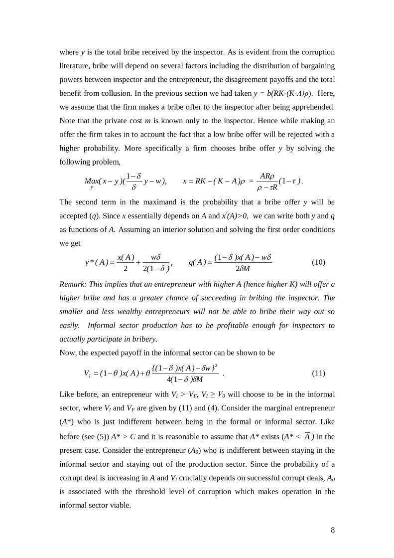
higher probability. More specifically a firm chooses bribe offer y by solving the
following problem,
)AK(RKx),wy)(yx(Max
y
1 = )(R
AR
1 .
The second term in the maximand is the probability that a bribe offer y will be
accepted (q). Since x essentially depends on A and x/(A)>0, we can write both y and q
as functions of A. Assuming an interior solution and solving the first order conditions
we get
Mw)A(x)()A(q,
)(w)A(x)A(*y
21
122
(10)
Remark: This implies that an entrepreneur with higher A (hence higher K) will offer a
higher bribe and has a greater chance of succeeding in bribing the inspector. The
smaller and less wealthy entrepreneurs will not be able to bribe their way out so
easily. Informal sector production has to be profitable enough for inspectors to
actually participate in bribery.
Now, the expected payoff in the informal sector can be shown to be
M)(}w)A(x){()A(x)(VI
14
112
. (11)
Like before, an entrepreneur with VI > VF, VI ≥ V0 will choose to be in the informal
sector, where VI and VF are given by (11) and (4). Consider the marginal entrepreneur
(A*) who is just indifferent between being in the formal or informal sector. Like
before (see (5)) A* > C and it is reasonable to assume that A* exists (A* < A ) in the
present case. Consider the entrepreneur (A0) who is indifferent between staying in the
informal sector and staying out of the production sector. Since the probability of a
corrupt deal is increasing in A and VI crucially depends on successful corrupt deals, A0
is associated with the threshold level of corruption which makes operation in the
informal sector viable.
9
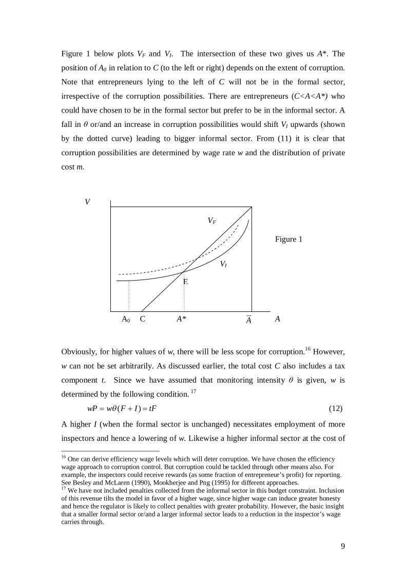
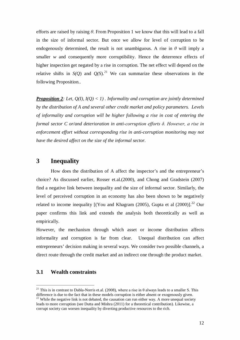
Figure 1 below plots VF and VI. The intersection of these two gives us A*. The
position of A0 in relation to C (to the left or right) depends on the extent of corruption.
Note that entrepreneurs lying to the left of C will not be in the formal sector,
irrespective of the corruption possibilities. There are entrepreneurs (C<A<A*) who
could have chosen to be in the formal sector but prefer to be in the informal sector. A
fall in θ or/and an increase in corruption possibilities would shift VI upwards (shown
by the dotted curve) leading to bigger informal sector. From (11) it is clear that
corruption possibilities are determined by wage rate w and the distribution of private
cost m.
Obviously, for higher values of w, there will be less scope for corruption.16 However,
w can not be set arbitrarily. As discussed earlier, the total cost C also includes a tax
component t. Since we have assumed that monitoring intensity θ is given, w is
determined by the following condition. 17
tFIFwwP )( (12)
A higher I (when the formal sector is unchanged) necessitates employment of more
inspectors and hence a lowering of w. Likewise a higher informal sector at the cost of 16 One can derive efficiency wage levels which will deter corruption. We have chosen the efficiency wage approach to corruption control. But corruption could be tackled through other means also. For example, the inspectors could receive rewards (as some fraction of entrepreneur’s profit) for reporting. See Besley and McLaren (1990), Mookherjee and Png (1995) for different approaches. 17 We have not included penalties collected from the informal sector in this budget constraint. Inclusion of this revenue tilts the model in favor of a higher wage, since higher wage can induce greater honesty and hence the regulator is likely to collect penalties with greater probability. However, the basic insight that a smaller formal sector or/and a larger informal sector leads to a reduction in the inspector’s wage carries through.
A
V
A
VI
VF
A* C
E
A0
Figure 1
10
formal sector (so that I + F is unchanged) will lead to a lower wage.18 From (10) it is
clear that a lower w in turn would mean a higher q for each level of A, provided q<1.
Hence informality extends the scope for corruption.
To capture the extent of corruption, it will be convenient to refer to the average
corruption level given by the following.
*A
A
dA)A(g)A(qI
Q0
1 (13)
Suppose q(A) = q (as in Section 2.2), then (13) implies that q = Q. Following the
previous discussion, it is clear that we can express the level of corruption as Q(S) and
SQ
> 0.
2.4 Joint determination: Informality and Corruption As discussed earlier, an entrepreneur’s payoff from being in the informal sector will
depend on the probability that it is able to bribe the inspector. As the level of
corruption rises the expected payoff from being in the informal sector is also higher.
Formally, informality and corruption will follow from decisions by entrepreneurs
(with different A) regarding the choice of sector and size of bribe offer, and decisions
by inspector (with different m) to accept the bribe or not. Given the distributions of A
and m, credit market parameters τ, ρ, and other policy parameters θ, , C, and t, we
can solve for informality and corruption. However, instead of formally deriving the
equilibrium, we use the following Figure to provide the basic intuition and heuristic
analysis.
18 It can be shown that we can not have a case where I rises but (I+F) falls significantly to raise w.
11
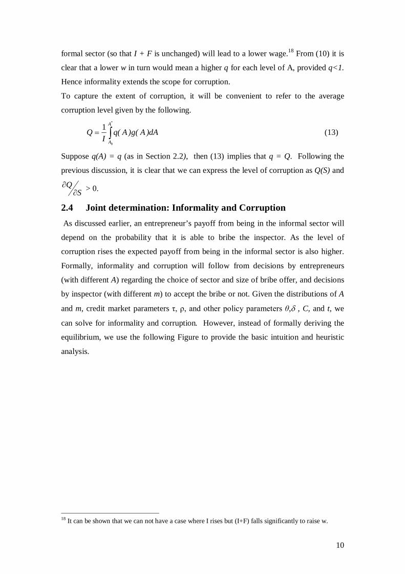
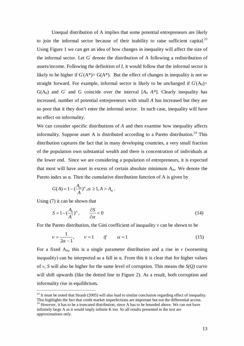
Figure 2 plots S(Q) and Q(S) showing the equilibrium levels of informality and
corruption (point E). Using (12) we argued that Q(S) is positively sloped. From (8) in
Section 2.2, it is clear that higher values of Q will lead to a bigger informal sector.
Hence S(Q) is also positively sloped. To guarantee that these two curves intersect (an
interior equilibrium point) we assume that Q(1) <1 and S(1) < 1. The first inequality is
always going to be satisfied for higher values of M. This is similar to the assumption
made in various models of corruption where a certain (however small) fraction of the
population is always honest. Likewise, the second inequality will follow from the fact
bribery is not costless. The entrepreneur in the informal sector will escape the
stipulated punishment with certainty, but will nonetheless pay a substantial bribe to do
so. Additionally, S(0) > Q(0).19
Figure 2 shows how levels of informality and corruption will change following
changes in exogenous parameters. Following a rise in C, keeping the level of
corruption the same, the relative size of informal sector goes up. This leads to an
upward shift in S(Q) (shown by the dotted line) resulting in higher informality and
corruption.20 Similarly, suppose anti-corruption efforts are more effective (δ is
higher) or the private cost of dismissal m goes up. This will lead to a shift in Q(S)
(shown by the dotted line) resulting in a fall in the levels of corruption and
informality. In some other instances both these curves will shift. Suppose enforcement
19 Note that Q(S) is not well defined at S = 0. One can use limited arguments here, we are referring to smallest possible informal sector share. 20 Usually, C is associated with extortion and bribery in the formal sector (i.e. Choi and Thum 2005), but this result shows that corruption in the informal sector is also affected by changes in C. These complementarities between different forms of corruption have not been modeled.
Q
S
1
S(Q)
Q(S)
Q*
S* E
Figure 2
12
efforts are raised by raising θ. From Proposition 1 we know that this will lead to a fall
in the size of informal sector. But once we allow for level of corruption to be
endogenously determined, the result is not unambiguous. A rise in θ will imply a
smaller w and consequently more corruptibility. Hence the deterrence effects of
higher inspection get negated by a rise in corruption. The net effect will depend on the
relative shifts in S(Q) and Q(S).21 We can summarize these observations in the
following Proposition..
Proposition 2: Let, Q(I), I(Q) < 1) . Informality and corruption are jointly determined
by the distribution of A and several other credit market and policy parameters. Levels
of informality and corruption will be higher following a rise in cost of entering the
formal sector C or/and deterioration in anti-corruption efforts δ. However, a rise in
enforcement effort without corresponding rise in anti-corruption monitoring may not
have the desired affect on the size of the informal sector.
3 Inequality How does the distribution of A affect the inspector’s and the entrepreneur’s
choice? As discussed earlier, Rosser et.al.(2000), and Chong and Gradstein (2007)
find a negative link between inequality and the size of informal sector. Similarly, the
level of perceived corruption in an economy has also been shown to be negatively
related to income inequality [(You and Khagram (2005), Gupta et al (2000)].22 Our
paper confirms this link and extends the analysis both theoretically as well as
empirically.
However, the mechanism through which asset or income distribution affects
informality and corruption is far from clear. Unequal distribution can affect
entrepreneurs’ decision making in several ways. We consider two possible channels, a
direct route through the credit market and an indirect one through the product market.
3.1 Wealth constraints
21 This is in contrast to Dabla-Norris et.al. (2008), where a rise in θ always leads to a smaller S. This difference is due to the fact that in these models corruption is either absent or exogenously given. 22 While the negative link is not debated, the causation can run either way. A more unequal society leads to more corruption (see Dutta and Mishra (2011) for a theoretical contribution). Likewise, a corrupt society can worsen inequality by diverting productive resources to the rich.
13
Unequal distribution of A implies that some potential entrepreneurs are likely
to join the informal sector because of their inability to raise sufficient capital.23
Using Figure 1 we can get an idea of how changes in inequality will affect the size of
the informal sector. Let G/ denote the distribution of A following a redistribution of
assets/income. Following the definition of I, it would follow that the informal sector is
likely to be higher if G/(A*)> G(A*). But the effect of changes in inequality is not so
straight forward. For example, informal sector is likely to be unchanged if G/(A0)>
G(A0) and G/ and G coincide over the interval [A0 A*]. Clearly inequality has
increased, number of potential entrepreneurs with small A has increased but they are
so poor that it they don’t enter the informal sector. In such case, inequality will have
no effect on informality.
We can consider specific distributions of A and then examine how inequality affects
informality. Suppose asset A is distributed according to a Pareto distribution.24 This
distribution captures the fact that in many developing countries, a very small fraction
of the population own substantial wealth and there is concentration of individuals at
the lower end. Since we are considering a population of entrepreneurs, it is expected
that most will have asset in excess of certain absolute minimum Am. We denote the
Pareto index as α. Then the cumulative distribution function of A is given by
mm AA
AAAG ,1,)(1)( .
Using (7) it can be shown that
0,)(1 *0
SAAS (14)
For the Pareto distribution, the Gini coefficient of inequality ν can be shown to be
11,12
1
if (15)
For a fixed Am, this is a single parameter distribution and a rise in ν (worsening
inequality) can be interpreted as a fall in α. From this it is clear that for higher values
of ν, S will also be higher for the same level of corruption. This means the S(Q) curve
will shift upwards (like the dotted line in Figure 2). As a result, both corruption and
informality rise in equilibrium. 23 It must be noted that Straub (2005) will also lead to similar conclusion regarding effect of inequality. This highlights the fact that credit market imperfections are important but not the differential access. 24 However, it has to be a truncated distribution, since A has to be bounded above. We can not have infinitely large A as it would imply infinite K too. So all results presented in the text are approximations only.
14
3.2 Informal sector profitability As discussed in previous sections, for the informal sector to be large,
profitability in this sector has to be high. But entrepreneurs in the informal sector do
not have access to benefits associated with various public goods and secure property
rights.25. What prevents informal sector profitability from being driven down? In this
Section we argue that greater inequality enhances profitability in the informal sector.
We argue that informal sector returns depend on the composition of entrepreneurs
operating in the formal sector. If the formal sector consists of highly productive/
efficient entrepreneurs, one expects informal sector returns to be lower. In the
presence of unequal distribution of A and imperfect credit market, some productive
but wealth constrained entrepreneurs are unable to enter the formal sector. As a result,
informal sector enjoys higher returns.
Consider the basic model of Section 2 with the following differences. Entrepreneurs
can be of two types depending on their abilities: high (h) and low (l). Let H and L
denote the measures of these two types. We also assume that credit market is non-
existent. Productivity of the h-type entrepreneur in the formal sector is given by Rh.
Productivity of the l-types in the formal sector and productivity of both types in the
informal sector is simply RI, Rh < RI. As discussed earlier RI depends on the number
of h-type entrepreneurs in the formal sector. In the informal sector, we consider the
simpler version of section 2.2 where the probability of meeting a corrupt inspector is
same for all entrepreneurs and is fixed at q. Assuming θ = 1, we can derive the
payoffs VF and VI as follows.
)(,..),( CARVARbqVCARV IFlIIhFh (16)
The h-type entrepreneurs with A≥ A*h will choose to be in the formal sector where
Ih
hh RbqR
CRA..
*
(17)
We can derive a similar condition for the l-type entrepreneurs. The number of h-type
formal sector entrepreneurs will be given by
25 Dabla-Norris et. al. (2008) note that informal sector is populated by less productive firms. It is clear that causality runs both ways. A firm is less productive because it is located in the informal sector. The reverse is also possible, only less productive firm prefer to join the informal sector.
15
A
Ah
h
dAAgHF*
)( (18)
Recall that RI = R(Fh ) and R/ < 0. Consider a situation where G(A*h ) is small. This
suggests a large Fh leading to a low RI. But a lower RI reduces A*h further and more h-
type entrepreneurs would join the formal sector. The informal sector will be populated
by some h-type (A< A*h ) and more l-types with A < C/(1-qb). However, a lower RI
implies that those with lower A will choose to be outside the production sector. In the
limiting case, Fh reaches its maximum (A*h→ C).
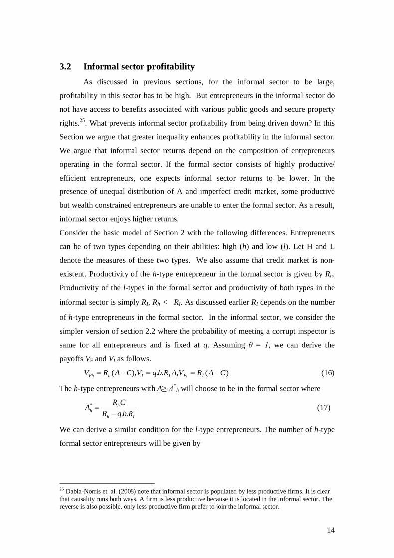
If the number of wealth-constrained entrepreneurs rises following a redistribution of
assets, the number of h-type entrepreneurs entering the formal sector shrinks
significantly. As Fh falls initially due to redistribution, RI increases leading to further
expansion of the informal sector and fall in Fh. The Figure below shows how the
informal sector grows following a change in distribution of A. The solid and dashed VI
lines show the payoffs to being in the informal sector before and after the
redistribution, respectively. The slopes of the two lines are different because
profitability is higher following the exit of some h-types after the redistribution. The
initial redistribution might have been small but the final effect on the size of the
informal sector is substantial.
We summarize the previous discussions in the following Proposition.
Proposition 3: A rise in inequality following an increase in the number of wealth
constrained entrepreneurs will lead to a bigger informal sector and more corruption.
A
V
A
VI
VF
A* C A*
VI Figure 3
16
4 Data and Empirical Analysis The World Bank Enterprise Surveys (WBES) which provided the data set used in this
study collect information (from the firm level surveys) about a host of questions that
include the business environment, how it is perceived by individual firms, how it
changes over time, and about the various constraints on firm performance and growth.
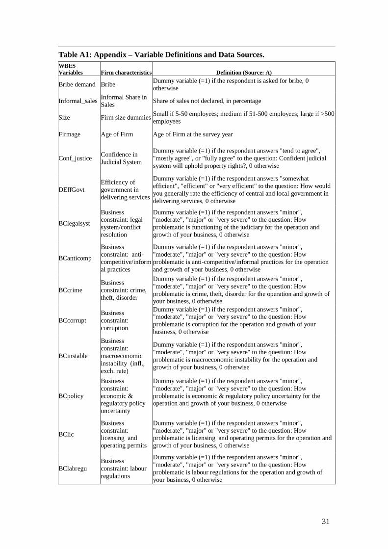
The WBES is not panel data, but repeated cross section26. The Appendix table A1
lists the variables from this data set that we have used in this study. The variables that
are worth special mention in the present context are Informal sales (as % age of total
sales) and Bribe demand which is a dummy that takes the value 1 if the firm has been
asked to pay a bribe and 0, otherwise. The data set, one of the largest of its kind, is a
cross country data set covering a range of developing and developed countries at
various stages of development. While the WBES data provides information on the
characteristics and attitudes of the individual firms surveyed, we supplemented this
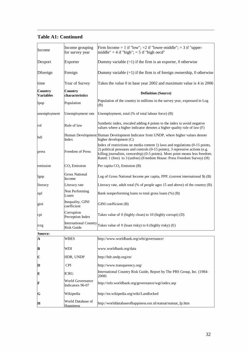
information by country level indicators obtained from a variety of sources that have
been listed in the second half of Appendix table A1. These include the macro
corruption perception and corruption risk indicators, Corruption Perception Index
(CPI) distributed by Transparency International and corruption component of
International Country Risk Guide (ICRG) supplied by Political Risk Services,
respectively, which have been widely used in recent studies.27 In our empirical work,
we arranged the CPI and ICRG variables such that higher values denote increased
corruption perception and corruption risk. It is important to note that while the
variable, Bribe demand, is a firm level characteristic that contains information on
whether a firm has been asked for a bribe or not, this is distinct from the country level
corruption indicators, CPI and ICRG, which measure the overall climate of corruption
in the country.
The estimations reported below were based on a pooling of the WBES data sets over
the period, 2002-2006. The list of countries by years and showing the number of firms
interviewed in each country is presented in Appendix table A2. Starting from a total
26 Further details are available from the World Bank website, http://www.enterprisesurveys.org/ . See also Batra et al. (2003) for description of the data and some of its principal features. Dabla-Norris et. al. (2008) use this data as well to study the determinants of informality. 27 See the following websites on details of these perception indictors: http://www.prsgroup.com/ and http://www.transparency.org/ .
17
of 27,086 observations, as recorded in Appendix Table A2, we lost observations with
the inclusion of the various determinants dropping down to 17606 observations which
dropped further to 10,883 observations with the inclusion of additional country level
characteristics.
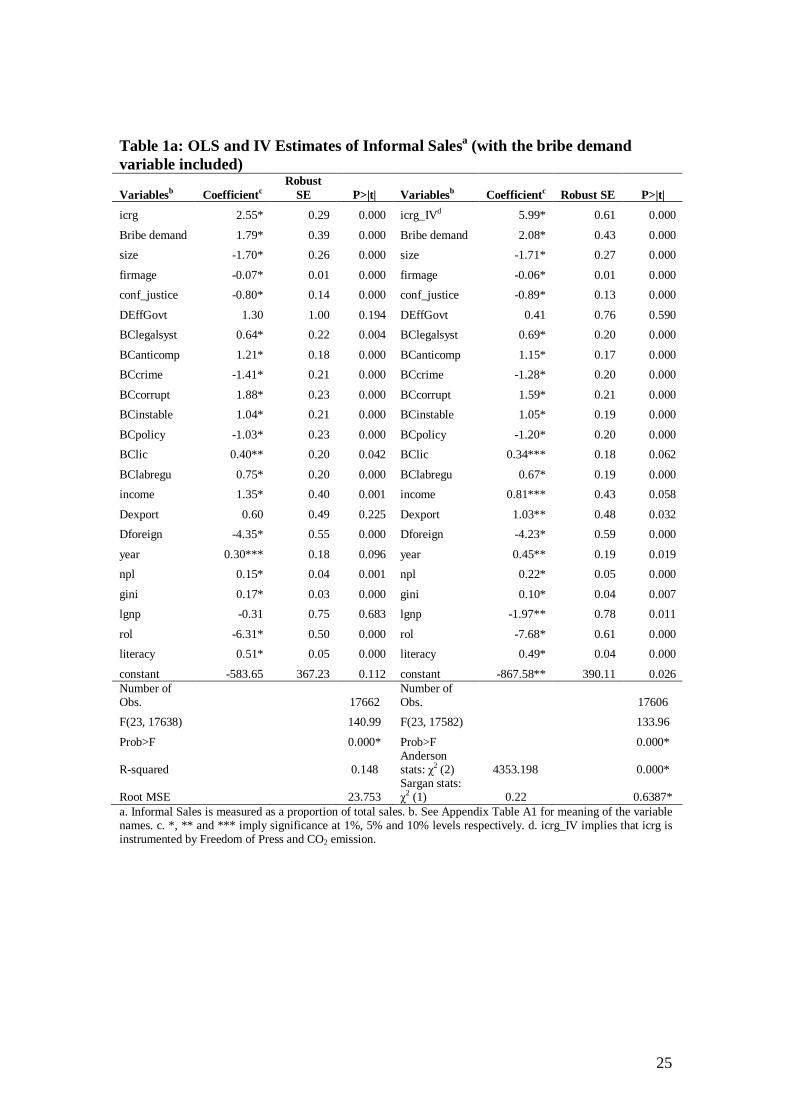
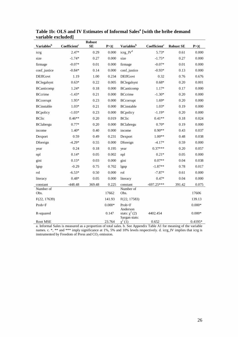
Tables 1a and 1b present the OLS and IV estimates of the regression of informal sales
( as % age of total sales) on a variety of firm characteristics and country level
indicators listed in Appendix table A1.The IV estimation was based on the treatment
of the corruption perception indicator, ICRG, for possible endogeneity. Tables 1a and
1b differ because while the former (table 1a) includes the bribe demand of the
individual firm as a determinant of that firm’s informal sales, the latter (table1b)
excludes this variable The tables also present the robust standard errors and the p-
values showing the significance of the estimates. The estimates are mostly well
determined.
Tables1a and 1b provide strong and robust support to the proposition on a positive
association between corruption perception and informal sales. In other words, firms
that operate in countries that are perceived to be at higher risk from corruption report,
ceteris paribus, a higher share of its sales as informal sales. It is worth noting that this
result is robust to the instrumentation of corruption perception by freedom of press
and CO2 emissions. The positive, large and statistically significant estimate of the
coefficient of the bribe demand variable in Table 1a suggests that a firm that has been
asked to pay a bribe will increase its undeclared sales as a proportion of its total sales
quite substantially. Income inequality, measured by Gini coefficient (gini) has a
strong and positive effect on informal sales. Consistent with the proposition28 derived
earlier, increasing inequality leads to a large increase in the size of the informal
sector. Another variable with a positive effect on informal sales and with some policy
significance is nonperforming loans (npl). This result suggests that in a deteriorating
credit environment caused by large default of loans due to their non performance the
informal sector will be larger. The qualitative results are generally robust between the
OLS and the IV estimates, i.e. with respect to the sign and significance of the
estimates, though the magnitude often changes. This is in line with the bias in the
OLS estimates from the treatment of the corruption perception variable (icrg) as an
28 Strictly speaking, the proposition relates to wealth inequality but, given the availability of data on wealth inequality for only a limited number of countries, we are using income inequality as a proxy for wealth inequality.
18
exogenous determinant. These tables also provide evidence on the validity of the
instruments used.
Other results from tables 1a, 1b include the feature that a firm’s perception of the
country’s legal system is a significant determinant of its decision on informal
operations. Increased confidence in the country’s justice system (conf_justice) will
encourage a firm to reduce informality and increase the share of formal sales. A firm
that considers the functioning of the country’s judiciary as not conducive to its
business operations (BClegalsyst) or, alternatively, views corruption as a business
impediment (BCcorrupt) will increase the share of its total sales that it chooses not to
declare. This is also true of firms that see labour regulations (BClabregu) as a
constraint on its business operations. Consistent with these results and that of Dabla-
Norris, et. al. (2008), the large and highly significant coefficient estimate of the rule
of law variable (ROL) suggests that firms operating in countries with superior quality
legal systems will declare a larger share of their sales or, alternatively, improved legal
systems will reduce informality. In other words, measures aimed at strengthening
legal institutions, stricter enforcement of justice and increased confidence in the
country’s judiciary are some of the most effective means of safeguarding the formal
sector and preventing informality.
Foreign owned firms are much less likely to go informal, but higher income firms and
those in the export business will have a higher informality. The more literate a
country, the higher is the size of the informal sector. Note however that this
paradoxical result could be due to the treatment of bribe demand as an exogenous
determinant of informal sales. As the following tables show, bribe demand is
significantly and negatively affected by the literacy rates. The overall message from
tables 1a and 1b is one of robustness of the qualitative picture on the effects of the
principal variables of interest on informal share of sales to the treatment of the macro
level corruption variable (icrg) as an exogenous or endogenous determinant in the
econometric specification. The evidence contained in Tables 1(a) and 1(b) provides
strong empirical support to the propositions in Sections 2 and 3.
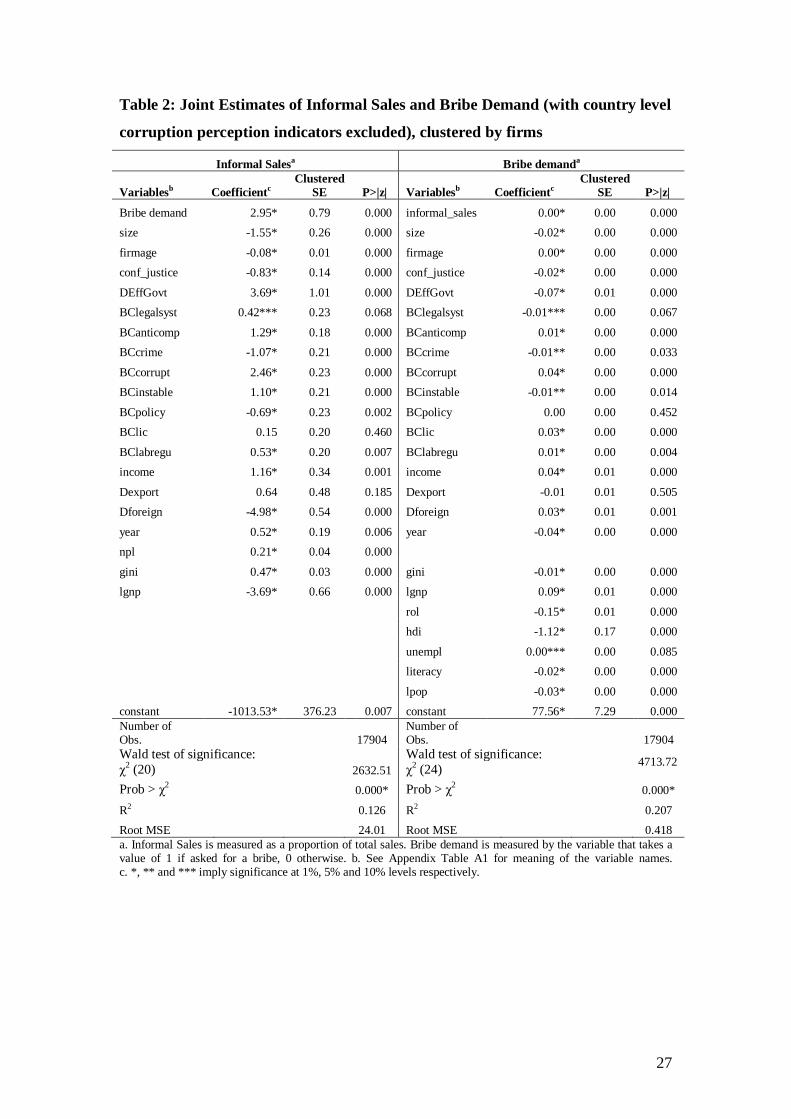
As discussed earlier, the positive correlation between bribe demand and informality
suggests that firms that are asked to pay bribes will declare a lower share of their
sales. However, this relationship can go the other way as well since firms that go
informal are more likely to receive bribe demands. To allow for this joint dependence,
and examine robustness of the results to the possible endogeneity of the bribe demand
19
variable, we performed joint estimation of informal sales and bribe demand consistent
with the discussion on their joint determination in Section 2.4. The results are
presented in Table 2 with the standard errors clustered by firms. Table 2 allows
comparison of the effects of the various determinants of the two forms of illegality.
Such a comparison suggests that the direction of the effect of the firm level
characteristics and the macro indicators on informal sales and bribe demands is the
same in most cases, but the magnitude of such effects is generally much larger for
informal sales. The principal result of Table 1a, namely, the positive impact of bribe
demand on informality is not only robust but the effect is actually stronger in Table 2
which allows for two way feedback between the two. Table 2 confirms the reverse
causation with informal sales having a positive and significant effect on bribe
demands though the effect is much weaker. Increasing confidence in the country’s
judicial system acts a brake on both forms of illegality extending the earlier result in
Table 1 from informality to corruption. The earlier result that rising inequality
increases informality is also robust between the two tables. It is also worth noting that
while inequality has a large, positive and significant effect on informal sales,
inequality has a negative and statistically significant effect on bribe demand, though
the effect is much weaker. The rule of law variable impacts negatively on the
corruption variable and this is passed on to informality through the positive
association between corruption and informality. The policy implication is clear- an
integrated approach to reducing both informality and corruption rests on a
strengthening of legal institutions and measures to increase confidence in the
country’s judiciary. An interesting point of difference between the two forms of
illegality is that, after controlling for the respondents’ characteristics and country
differences, while there has an increase in informality there has been a decline in
business corruption.
Table 2 excludes several of the country level variables from the informal sales
equation that is reported on the left hand side, though they appear as determinants in
the bribe demand equation. Prominent examples of such omissions include the rule of
law (rol) and human development index (hdi). In other words, these country
characteristics are assumed to have an impact on informal sales only through the bribe
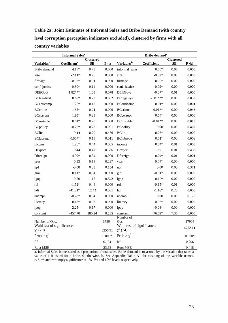
demand variable. Table 2a examines robustness of the evidence in table 2 by
including all the principal country level variables in the informal sales equation just as
they do in the bribe demand equation. In other words, all the country indicators have
20
both a direct effect and indirect effect on informal sales. The standard errors are
clustered by firms as in table 2. A comparison of tables 2 and 2a establishes
robustness of the principal result of table 2, namely, the positive and mutually
reinforcing relationship between informal sales and bribe demand. In fact, the impact
of bribe demand on informal sales strengthens considerably on the inclusion of the
country level variables in the equation for informal sales. The rule of law (rol), human
development index (hdi) and the unemployment rate (unempl) variables, that were all
excluded from the informal sales equation reported in table 2, are seen from the left
hand side of table 2 (a) to have a significantly negative direct impact on informal
sales. It is worth noting from the right hand side of table 2 (a) that the first two
country characteristics (rol, hdi) also have a significantly negative impact on bribe
demand, though the size of the coefficients is smaller compared to those in the
informal sales equation. Literacy has reverse impacts on informal sales and bribe
demand, positive in case of the former, negative in case of the latter. The coefficient
estimates in the bribe demand equation in table 2a are nearly all identical to those in
table 2, ie. the results in the bribe demand equation are robust to the expanded list of
country level regressors used in the informal sales equation
Tables 2, 2a both suffer from the limitation that while the joint estimations consider
the effect of micro level business corruption in the form of the WBES variable, bribe
demands, on informal sales, they do not control for the corruption perception of the
country at the macro level. To do so, we repeated the joint estimation with the
corruption perception variables, ICRG and CPI, introduced as additional regressors,
on the right hand size of the informal sales and corruption equations, respectively. The
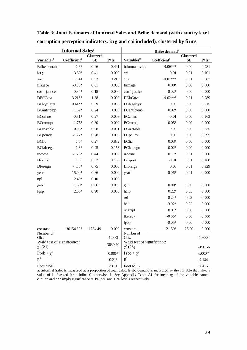
results corresponding to Tables 2, 2a are reported in Tables 3, 3a, respectively.
The positive association between corruption and informal sales manifests itself
through the large and statistically significant impact of ICRG on informal sales. In
other words, and consistent with tables 1a,1b, firms operating in countries with higher
perceived risk of corruption are likely to experience greater informality. Note,
however, that on the introduction of the country wide indicator, icrg, the effect of the
firm level bribe demand variable in the informal sales equation now weakens to
statistical insignificance. This has the policy message that, in countries which are not
regarded as being at high risk from corruption, bribe demands on the individual firms
do not have any impact on the firm’s decision on informality. It is the overall
corruption perception of a country that matters in driving informality, not so much the
21
bribe demands made to the individual firms. In contrast, controlling for macro level
corruption as measured by the corruption perception indicator (cpi) and the other
determinants, increased informality does lead to significantly higher bribe demands on
the firms. Most of the principal results on informality, for example, rising inequality
increases informality, increased confidence in the country’s judiciary and an
improvement in the credit situation brought about by a reduction in non performing
bank loans reduces informality, is seen from Tables 1 and 3 to be robust between the
single equation and the simultaneous equation estimates. Note from Table 3 that rising
inequality as measured by the Gini leads to an increase in both informal sales and
bribe demands as stated in our Proposition 3, but the effect on the latter is much
weaker.
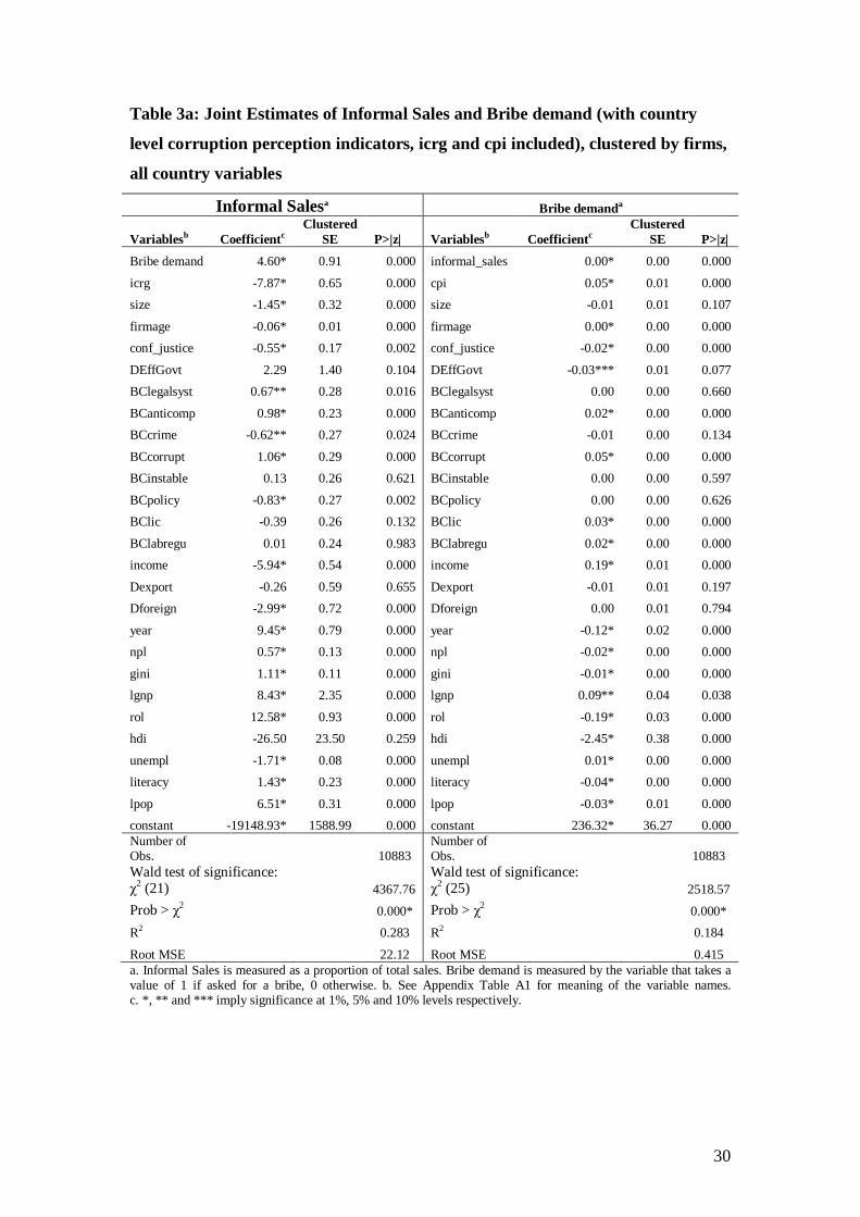
Table 3a shows that the sign, size and significance of the impact of corruption risk
(icrg) on informal sales are highly sensitive to the inclusion of the additional country
indicators as regressors in the informal sales equation. Controlling for the other
indicators, table 3a confirms the results in tables 2, 2(a) that bribe demand has a
positive impact on informal sales and vice versa as well. In contrast, once we control
for bribe demand and the expanded list of country characteristics, informal sales will
be lower in countries which are considered to be at high risk from corruption. The
estimated coefficients reported on the right hand side of tables 3 and 3 (a) are virtually
identical. The result that comes out consistently from these tables is one of a positive
and mutually reinforcing relationship between bribe demand and informal sales.
Another remarkably robust result is that, ceteris paribus, increasing inequality has a
large and positive impact on informal sales, consistent with the analytical discussion
of this paper. Again, as the earlier discussion suggests, a deteriorating credit situation,
as reflected in an increase in nonperforming bank loans (npl), will tend to increase
informal sales. This result is seen most clearly from the large and statistically
significant positive coefficient estimate of npl on the left hand side of tables 3 and 3
(a). The empirical results are subject to the qualification that while they establish
association they do not necessarily indicate causation. That is an area for further
research.

22
5. Conclusion
The principal objective has been to look at the determinants of the size of the informal
sector in developing countries. Large informal sectors are predominant in developing
countries and corruption is also pervasive in many of these countries. This is not a
simple coincidence; the paper proposes an analytical model where corruption and
informality are closely linked. In fact corruption and informality are jointly
determined by a common set of variables. Our empirical exercises using firm level
data support this approach.
While we do not dispute several earlier observations that higher tax rates in the formal
sector and inefficient regulations drive firms to the informal sectors, these
observations fail to explain why firms in the informal sector find it viable and in
many cases profitable to operate. Corruption in the informal sector allows the
informal sector firms to enjoy greater protection from enforcement and consequently
higher profits. Corruptible inspectors, in turn, thrive when there is a large informal
sector. For a fixed size of formal sector, a larger informal sector implies poorer
enforcement effort and lower efficiency wages for the inspectors.
Corruption and informality complement each other and are jointly determined by
several firm level as well as economy level variables like levels of development,
literacy levels. Our key contribution lies in exploring the link between informality and
inequality. Our theoretical model as well empirical exercises focus on wealth/income
inequality as a key determinant. High degree of inequality leads to a bigger informal
sector.
There are different ways in which inequality can affect informality and corruption.
The first one is the most obvious and direct route where greater wealth inequality in
the sense of large number wealth constrained entrepreneurs can lead to larger informal
sector. Formal sector is normally associated with larger fixed costs and these wealth
constrained individuals are forced to join the informal sector in the absence of well
functioning credit markets. The second (indirect) route is through the product market.
We argue that greater inequality limits the entry of productive but wealth constrained
firms in the formal sector. As a result, informal sector enjoys higher returns.29 The
29 In a related paper Mishra (2011) argues, in a model with differentiated products, that informal sector returns are likely to high due to a strong demand for informal sector goods emanating from distributional issues. Greater inequality in income distribution of the consumers will mean bigger demand and profitability for the informal sector.
23
empirical exercises show that this relation between informality and inequality is
indeed quite robust.
References Ades, A., Di-Tella, R., 1999. Rents, competition and corruptio. American Economic
Review, 89( ) 982-93. Batra, G., Kaufmann, D., Stone, A.H., 2003. The firms speak: what the World
Business Environment Survey tells us about constraints on private sector development. Working Paper, World Bank.
Besley, T., Maclaren, J., 1993. Taxes and bribery: The role of wage incentives. Economic Journal, 103(416), 119-141.
Bose, P., Echazu,L., 2007. Corruption with heterogenous enforcement agents in the shadow economy. Journal of Institutional and Theoretical Economics. 163, 285-296.
Choi, J., Thum, M., 2005. Corruption and the shadow economy. International Economic Review 46, 817-836.
Chong, A., Gradstein, M., 2007. Inequality and Informality. Journal of Public Economics 91, 159-179.
Cule, M., Fulton, M., 2005. Some implications of the unofficial economy. Economics Letters 89, 207-211.
Dabla-Norris, E., Gradstein, M., Inchauste, G., 2008. What causes firms to hide output? The determinants of informality. Journal of Development Economics 85, 1-27.
De Mel, S., McKenzie, D., Woodruff, C., 2010, What is the cost of formality? Mimeo, University of Warwick, UK. Djankov, S., La-Porta, R., Lopez-de-Silanes, F., Shleifer, A., 2002. The regulation of
entry. Quarterly Journal of Economics, 117, 1-37. Dutta, I., Mishra, A., 2011. Does inequality foster corruption? Journal of Public
Economic Theory, forthcoming Friedman, E., Johnson S., Kaufmann, D., Zoido-Lobaton, P., 2000. Dodging the
grabbing hand: The determinants of unofficial activity in 69 countries. Journal of Public Economics, 76, 459-493.
Gupta, S., Davoodi, H., Alonso-Terme, R., 2002. Does corruption affect inequality and poverty? Economics of Governance , 3, 23-45.
Johnson, S., Kaufmann, D., Zoido-Lobaton, P., 1998. Regulatory discretion and the unofficial economy. American Economic Review Papers and Proceedings 88,387-392.
Loayza, N.,1996. The economics of the informal sector. Carnegie-Rochester Conference Series on Public Policy 45, 129-162.
Matsuyama, K., 2000, Endogenous Inequality. Review of Economic Studies 67, 743-759. McKenzie, D., Sakho, Y.S., 2010. Does it pay firms to register for taxes? Journal of Development Economics, 91, 15-24 Mishra, A., 1995. Economics of Corruption. Oxford University Press, New Delhi.
24
Mishra, A., 2011, Informality and Inequality: The product market channel, mimeo, University of Bath, UK. Mookherjee, D., Png, I., 1995. Corruptible law enforcers: how should they be
compensated. Economic Journal, 105, 149-159. Rauch, J., 1991. Modeling the informal sector formally. Journal of Development
Economics 35, 33-47. Rosser, J.B. Jr, Rosser, M.V., Ahmed, E., 2000. Income inequality and the informal
economy in transition countries. Journal of Comparative Economics 28, 156-171. Samuel, A., Alger, A.,2010. Corruption, the informal sector and foreign aid in weak
states. mimeo, Loyola University, Baltimore, MD 21210. Schneider, F., Ernste, D., 2000. Shadow economies: Size, causes and consequences.
Journal of Economic Literature. 38, 77-114. Straub, S., 2005. Informal sector: the credit market channel. Journal of Development
Economics 78, 299-321. You, J-S., Khagram, S., 2005. A comparative study of inequality and corruption,
American Sociological Review 70, 136-157.
25
Table 1a: OLS and IV Estimates of Informal Salesa (with the bribe demand variable included)
Variablesb Coefficientc Robust
SE P>|t| Variablesb Coefficientc Robust SE P>|t|
icrg 2.55* 0.29 0.000 icrg_IVd 5.99* 0.61 0.000
Bribe demand 1.79* 0.39 0.000 Bribe demand 2.08* 0.43 0.000 size -1.70* 0.26 0.000 size -1.71* 0.27 0.000
firmage -0.07* 0.01 0.000 firmage -0.06* 0.01 0.000 conf_justice -0.80* 0.14 0.000 conf_justice -0.89* 0.13 0.000
DEffGovt 1.30 1.00 0.194 DEffGovt 0.41 0.76 0.590 BClegalsyst 0.64* 0.22 0.004 BClegalsyst 0.69* 0.20 0.000
BCanticomp 1.21* 0.18 0.000 BCanticomp 1.15* 0.17 0.000 BCcrime -1.41* 0.21 0.000 BCcrime -1.28* 0.20 0.000
BCcorrupt 1.88* 0.23 0.000 BCcorrupt 1.59* 0.21 0.000 BCinstable 1.04* 0.21 0.000 BCinstable 1.05* 0.19 0.000
BCpolicy -1.03* 0.23 0.000 BCpolicy -1.20* 0.20 0.000 BClic 0.40** 0.20 0.042 BClic 0.34*** 0.18 0.062
BClabregu 0.75* 0.20 0.000 BClabregu 0.67* 0.19 0.000 income 1.35* 0.40 0.001 income 0.81*** 0.43 0.058
Dexport 0.60 0.49 0.225 Dexport 1.03** 0.48 0.032 Dforeign -4.35* 0.55 0.000 Dforeign -4.23* 0.59 0.000
year 0.30*** 0.18 0.096 year 0.45** 0.19 0.019 npl 0.15* 0.04 0.001 npl 0.22* 0.05 0.000
gini 0.17* 0.03 0.000 gini 0.10* 0.04 0.007 lgnp -0.31 0.75 0.683 lgnp -1.97** 0.78 0.011
rol -6.31* 0.50 0.000 rol -7.68* 0.61 0.000 literacy 0.51* 0.05 0.000 literacy 0.49* 0.04 0.000
constant -583.65 367.23 0.112 constant -867.58** 390.11 0.026 Number of Obs. 17662
Number of Obs.
17606
F(23, 17638) 140.99 F(23, 17582) 133.96
Prob>F 0.000* Prob>F 0.000*
R-squared 0.148 Anderson stats: χ2 (2) 4353.198
0.000*
Root MSE 23.753 Sargan stats: χ2 (1) 0.22
0.6387*
a. Informal Sales is measured as a proportion of total sales. b. See Appendix Table A1 for meaning of the variable names. c. *, ** and *** imply significance at 1%, 5% and 10% levels respectively. d. icrg_IV implies that icrg is instrumented by Freedom of Press and CO2 emission.
26
Table 1b: OLS and IV Estimates of Informal Salesa [with the bribe demand variable excluded]
Variablesb Coefficientc Robust
SE P>|t| Variablesb Coefficientc Robust SE P>|t|
icrg 2.47* 0.29 0.000 icrg_IVd 5.73* 0.61 0.000 size -1.74* 0.27 0.000 size -1.75* 0.27 0.000
firmage -0.07* 0.01 0.000 firmage -0.07* 0.01 0.000 conf_justice -0.84* 0.14 0.000 conf_justice -0.93* 0.13 0.000
DEffGovt 1.19 1.00 0.234 DEffGovt 0.32 0.76 0.676 BClegalsyst 0.63* 0.22 0.005 BClegalsyst 0.68* 0.20 0.001
BCanticomp 1.24* 0.18 0.000 BCanticomp 1.17* 0.17 0.000 BCcrime -1.43* 0.21 0.000 BCcrime -1.30* 0.20 0.000
BCcorrupt 1.95* 0.23 0.000 BCcorrupt 1.69* 0.20 0.000 BCinstable 1.03* 0.21 0.000 BCinstable 1.03* 0.19 0.000
BCpolicy -1.03* 0.23 0.000 BCpolicy -1.19* 0.20 0.000 BClic 0.46** 0.20 0.019 BClic 0.41** 0.18 0.024
BClabregu 0.77* 0.20 0.000 BClabregu 0.70* 0.19 0.000 income 1.40* 0.40 0.000 income 0.90** 0.43 0.037
Dexport 0.59 0.49 0.231 Dexport 1.00** 0.48 0.038 Dforeign -4.29* 0.55 0.000 Dforeign -4.17* 0.59 0.000
year 0.24 0.18 0.195 year 0.37*** 0.20 0.057 npl 0.14* 0.05 0.002 npl 0.21* 0.05 0.000
gini 0.15* 0.03 0.000 gini 0.07** 0.04 0.038 lgnp -0.29 0.75 0.702 lgnp -1.87** 0.78 0.017
rol -6.53* 0.50 0.000 rol -7.87* 0.61 0.000 literacy 0.48* 0.05 0.000 literacy 0.47* 0.04 0.000
constant -448.48 369.48 0.225 constant -697.25*** 391.42 0.075 Number of Obs. 17662
Number of Obs.
17606
F(22, 17639) 141.93 F(22, 17583) 139.13 Prob>F 0.000* Prob>F 0.000*
R-squared 0.147 Anderson stats: χ2 (2) 4402.454
0.000*
Root MSE 23.764 Sargan stats: χ2 (1) 0.652
0.4195*
a. Informal Sales is measured as a proportion of total sales. b. See Appendix Table A1 for meaning of the variable names. c. *, ** and *** imply significance at 1%, 5% and 10% levels respectively. d. icrg_IV implies that icrg is instrumented by Freedom of Press and CO2 emission.
27
Table 2: Joint Estimates of Informal Sales and Bribe Demand (with country level
corruption perception indicators excluded), clustered by firms
Informal Salesa Bribe demanda
Variablesb Coefficientc Clustered
SE P>|z| Variablesb Coefficientc Clustered
SE P>|z|
Bribe demand 2.95* 0.79 0.000 informal_sales 0.00* 0.00 0.000 size -1.55* 0.26 0.000 size -0.02* 0.00 0.000
firmage -0.08* 0.01 0.000 firmage 0.00* 0.00 0.000 conf_justice -0.83* 0.14 0.000 conf_justice -0.02* 0.00 0.000
DEffGovt 3.69* 1.01 0.000 DEffGovt -0.07* 0.01 0.000 BClegalsyst 0.42*** 0.23 0.068 BClegalsyst -0.01*** 0.00 0.067
BCanticomp 1.29* 0.18 0.000 BCanticomp 0.01* 0.00 0.000 BCcrime -1.07* 0.21 0.000 BCcrime -0.01** 0.00 0.033
BCcorrupt 2.46* 0.23 0.000 BCcorrupt 0.04* 0.00 0.000 BCinstable 1.10* 0.21 0.000 BCinstable -0.01** 0.00 0.014
BCpolicy -0.69* 0.23 0.002 BCpolicy 0.00 0.00 0.452 BClic 0.15 0.20 0.460 BClic 0.03* 0.00 0.000
BClabregu 0.53* 0.20 0.007 BClabregu 0.01* 0.00 0.004 income 1.16* 0.34 0.001 income 0.04* 0.01 0.000
Dexport 0.64 0.48 0.185 Dexport -0.01 0.01 0.505 Dforeign -4.98* 0.54 0.000 Dforeign 0.03* 0.01 0.001
year 0.52* 0.19 0.006 year -0.04* 0.00 0.000 npl 0.21* 0.04 0.000
gini 0.47* 0.03 0.000 gini -0.01* 0.00 0.000 lgnp -3.69* 0.66 0.000 lgnp 0.09* 0.01 0.000
rol -0.15* 0.01 0.000 hdi -1.12* 0.17 0.000
unempl 0.00*** 0.00 0.085 literacy -0.02* 0.00 0.000
lpop -0.03* 0.00 0.000 constant -1013.53* 376.23 0.007 constant 77.56* 7.29 0.000 Number of Obs. 17904
Number of Obs. 17904
Wald test of significance: χ2 (20) 2632.51
Wald test of significance: χ2 (24) 4713.72
Prob > χ2 0.000* Prob > χ2 0.000*
R2 0.126 R2 0.207 Root MSE 24.01 Root MSE 0.418 a. Informal Sales is measured as a proportion of total sales. Bribe demand is measured by the variable that takes a value of 1 if asked for a bribe, 0 otherwise. b. See Appendix Table A1 for meaning of the variable names. c. *, ** and *** imply significance at 1%, 5% and 10% levels respectively.
28
Table 2a: Joint Estimates of Informal Sales and Bribe Demand (with country
level corruption perception indicators excluded), clustered by firms with all
country variables
Informal Salesa Bribe demanda
Variablesb Coefficientc Clustered
SE P>|z| Variablesb Coefficientc Clustered
SE P>|z|
Bribe demand 4.18* 0.78 0.000 informal_sales 0.00* 0.00 0.000
size -2.11* 0.25 0.000 size -0.02* 0.00 0.000 firmage -0.06* 0.01 0.000 firmage 0.00* 0.00 0.000
conf_justice -0.80* 0.14 0.000 conf_justice -0.02* 0.00 0.000 DEffGovt 1.82*** 1.03 0.078 DEffGovt -0.07* 0.01 0.000
BClegalsyst 0.69* 0.23 0.002 BClegalsyst -0.01*** 0.00 0.053 BCanticomp 1.28* 0.18 0.000 BCanticomp 0.01* 0.00 0.001
BCcrime -1.35* 0.21 0.000 BCcrime -0.01** 0.00 0.048 BCcorrupt 1.95* 0.23 0.000 BCcorrupt 0.04* 0.00 0.000
BCinstable 0.81* 0.20 0.000 BCinstable -0.01** 0.00 0.013 BCpolicy -0.76* 0.23 0.001 BCpolicy 0.00 0.00 0.407
BClic 0.14 0.20 0.486 BClic 0.03* 0.00 0.000 BClabregu 0.50** 0.19 0.011 BClabregu 0.01* 0.00 0.006
income 1.26* 0.44 0.005 income 0.04* 0.01 0.000 Dexport 0.44 0.47 0.356 Dexport -0.01 0.01 0.498
Dforeign -4.09* 0.54 0.000 Dforeign 0.04* 0.01 0.001 year 0.23 0.19 0.227 year -0.04* 0.00 0.000
npl -0.08 0.05 0.154 npl 0.00 0.00 0.371 gini 0.14* 0.04 0.000 gini -0.01* 0.00 0.000
lgnp 0.70 1.15 0.542 lgnp 0.10* 0.02 0.000 rol -1.72* 0.48 0.000 rol -0.15* 0.01 0.000
hdi -41.81* 12.42 0.001 hdi -1.16* 0.20 0.000 unempl -0.28* 0.04 0.000 unempl 0.00 0.00 0.170
literacy 0.45* 0.08 0.000 literacy -0.02* 0.00 0.000 lpop 2.25* 0.17 0.000 lpop -0.03* 0.00 0.000
constant -457.70 385.24 0.235 constant 76.09* 7.36 0.000
Number of Obs. 17904 Number of Obs. 17904
Wald test of significance: χ2 (20) 3356.91
Wald test of significance: χ2 (24) 4752.11
Prob > χ2 0.000* Prob > χ2 0.000*
R2 0.154 R2 0.206 Root MSE 23.63 Root MSE 0.418 a. Informal Sales is measured as a proportion of total sales. Bribe demand is measured by the variable that takes a value of 1 if asked for a bribe, 0 otherwise. b. See Appendix Table A1 for meaning of the variable names. c. *, ** and *** imply significance at 1%, 5% and 10% levels respectively.
29
Table 3: Joint Estimates of Informal Sales and Bribe demand (with country level
corruption perception indicators, icrg and cpi included), clustered by firms Informal Salesa Bribe demanda
Variablesb Coefficientc Clustered
SE P>|z| Variablesb Coefficientc Clustered
SE P>|z|
Bribe demand -0.66 0.96 0.491 informal_sales 0.00*** 0.00 0.081 icrg 3.60* 0.41 0.000 cpi 0.01 0.01 0.101
size -0.41 0.33 0.215 size -0.01*** 0.01 0.087 firmage -0.08* 0.01 0.000 firmage 0.00* 0.00 0.000
conf_justice -0.84* 0.18 0.000 conf_justice -0.02* 0.00 0.000 DEffGovt 3.21** 1.38 0.020 DEffGovt -0.02*** 0.01 0.089
BClegalsyst 0.61** 0.29 0.036 BClegalsyst 0.00 0.00 0.615 BCanticomp 1.62* 0.24 0.000 BCanticomp 0.02* 0.00 0.000
BCcrime -0.81* 0.27 0.003 BCcrime -0.01 0.00 0.163 BCcorrupt 1.75* 0.30 0.000 BCcorrupt 0.05* 0.00 0.000
BCinstable 0.95* 0.28 0.001 BCinstable 0.00 0.00 0.735 BCpolicy -1.27* 0.28 0.000 BCpolicy 0.00 0.00 0.695
BClic 0.04 0.27 0.882 BClic 0.03* 0.00 0.000 BClabregu 0.36 0.25 0.153 BClabregu 0.02* 0.00 0.000
income -1.78* 0.44 0.000 income 0.17* 0.01 0.000 Dexport 0.83 0.62 0.185 Dexport -0.01 0.01 0.168
Dforeign -4.53* 0.75 0.000 Dforeign 0.00 0.01 0.929 year 15.00* 0.86 0.000 year -0.06* 0.01 0.000
npl 2.49* 0.10 0.000 gini 1.68* 0.06 0.000 gini 0.00* 0.00 0.000
lgnp 2.65* 0.90 0.003 lgnp 0.22* 0.03 0.000 rol -0.24* 0.03 0.000
hdi -3.02* 0.35 0.000 unempl 0.01* 0.00 0.000
literacy -0.05* 0.00 0.000 lpop -0.05* 0.00 0.000
constant -30154.39* 1734.49 0.000 constant 121.50* 25.90 0.000 Number of Obs. 10883
Number of Obs. 10883
Wald test of significance: χ2 (21) 3030.20 Wald test of significance:
χ2 (25) 2450.56 Prob > χ2 0.000* Prob > χ2 0.000* R2 0.218 R2 0.184
Root MSE 23.11 Root MSE 0.415 a. Informal Sales is measured as a proportion of total sales. Bribe demand is measured by the variable that takes a value of 1 if asked for a bribe, 0 otherwise. b. See Appendix Table A1 for meaning of the variable names. c. *, ** and *** imply significance at 1%, 5% and 10% levels respectively.
30
Table 3a: Joint Estimates of Informal Sales and Bribe demand (with country
level corruption perception indicators, icrg and cpi included), clustered by firms,
all country variables Informal Salesa Bribe demanda
Variablesb Coefficientc Clustered
SE P>|z| Variablesb Coefficientc Clustered
SE P>|z|
Bribe demand 4.60* 0.91 0.000 informal_sales 0.00* 0.00 0.000
icrg -7.87* 0.65 0.000 cpi 0.05* 0.01 0.000 size -1.45* 0.32 0.000 size -0.01 0.01 0.107
firmage -0.06* 0.01 0.000 firmage 0.00* 0.00 0.000 conf_justice -0.55* 0.17 0.002 conf_justice -0.02* 0.00 0.000
DEffGovt 2.29 1.40 0.104 DEffGovt -0.03*** 0.01 0.077 BClegalsyst 0.67** 0.28 0.016 BClegalsyst 0.00 0.00 0.660
BCanticomp 0.98* 0.23 0.000 BCanticomp 0.02* 0.00 0.000 BCcrime -0.62** 0.27 0.024 BCcrime -0.01 0.00 0.134
BCcorrupt 1.06* 0.29 0.000 BCcorrupt 0.05* 0.00 0.000 BCinstable 0.13 0.26 0.621 BCinstable 0.00 0.00 0.597
BCpolicy -0.83* 0.27 0.002 BCpolicy 0.00 0.00 0.626 BClic -0.39 0.26 0.132 BClic 0.03* 0.00 0.000
BClabregu 0.01 0.24 0.983 BClabregu 0.02* 0.00 0.000 income -5.94* 0.54 0.000 income 0.19* 0.01 0.000
Dexport -0.26 0.59 0.655 Dexport -0.01 0.01 0.197 Dforeign -2.99* 0.72 0.000 Dforeign 0.00 0.01 0.794
year 9.45* 0.79 0.000 year -0.12* 0.02 0.000 npl 0.57* 0.13 0.000 npl -0.02* 0.00 0.000
gini 1.11* 0.11 0.000 gini -0.01* 0.00 0.000 lgnp 8.43* 2.35 0.000 lgnp 0.09** 0.04 0.038
rol 12.58* 0.93 0.000 rol -0.19* 0.03 0.000 hdi -26.50 23.50 0.259 hdi -2.45* 0.38 0.000
unempl -1.71* 0.08 0.000 unempl 0.01* 0.00 0.000 literacy 1.43* 0.23 0.000 literacy -0.04* 0.00 0.000
lpop 6.51* 0.31 0.000 lpop -0.03* 0.01 0.000 constant -19148.93* 1588.99 0.000 constant 236.32* 36.27 0.000 Number of Obs. 10883
Number of Obs. 10883
Wald test of significance: χ2 (21) 4367.76
Wald test of significance: χ2 (25) 2518.57
Prob > χ2 0.000* Prob > χ2 0.000* R2 0.283 R2 0.184
Root MSE 22.12 Root MSE 0.415 a. Informal Sales is measured as a proportion of total sales. Bribe demand is measured by the variable that takes a value of 1 if asked for a bribe, 0 otherwise. b. See Appendix Table A1 for meaning of the variable names. c. *, ** and *** imply significance at 1%, 5% and 10% levels respectively.
31
Table A1: Appendix – Variable Definitions and Data Sources. WBES Variables Firm characteristics Definition (Source: A)
Bribe demand Bribe Dummy variable (=1) if the respondent is asked for bribe, 0 otherwise
Informal_sales Informal Share in Sales Share of sales not declared, in percentage
Size Firm size dummies Small if 5-50 employees; medium if 51-500 employees; large if >500 employees
Firmage Age of Firm Age of Firm at the survey year
Conf_justice Confidence in Judicial System
Dummy variable (=1) if the respondent answers "tend to agree", "mostly agree", or "fully agree" to the question: Confident judicial system will uphold property rights?, 0 otherwise
DEffGovt Efficiency of government in delivering services
Dummy variable (=1) if the respondent answers "somewhat efficient", "efficient" or "very efficient" to the question: How would you generally rate the efficiency of central and local government in delivering services, 0 otherwise
BClegalsyst
Business constraint: legal system/conflict resolution
Dummy variable (=1) if the respondent answers "minor", "moderate", "major" or "very severe" to the question: How problematic is functioning of the judiciary for the operation and growth of your business, 0 otherwise
BCanticomp
Business constraint: anti-competitive/informal practices
Dummy variable (=1) if the respondent answers "minor", "moderate", "major" or "very severe" to the question: How problematic is anti-competitive/informal practices for the operation and growth of your business, 0 otherwise
BCcrime Business constraint: crime, theft, disorder
Dummy variable (=1) if the respondent answers "minor", "moderate", "major" or "very severe" to the question: How problematic is crime, theft, disorder for the operation and growth of your business, 0 otherwise
BCcorrupt Business constraint: corruption
Dummy variable (=1) if the respondent answers "minor", "moderate", "major" or "very severe" to the question: How problematic is corruption for the operation and growth of your business, 0 otherwise
BCinstable
Business constraint: macroeconomic instability (infl., exch. rate)
Dummy variable (=1) if the respondent answers "minor", "moderate", "major" or "very severe" to the question: How problematic is macroeconomic instability for the operation and growth of your business, 0 otherwise
BCpolicy
Business constraint: economic & regulatory policy uncertainty
Dummy variable (=1) if the respondent answers "minor", "moderate", "major" or "very severe" to the question: How problematic is economic & regulatory policy uncertainty for the operation and growth of your business, 0 otherwise
BClic
Business constraint: licensing and operating permits
Dummy variable (=1) if the respondent answers "minor", "moderate", "major" or "very severe" to the question: How problematic is licensing and operating permits for the operation and growth of your business, 0 otherwise
BClabregu Business constraint: labour regulations
Dummy variable (=1) if the respondent answers "minor", "moderate", "major" or "very severe" to the question: How problematic is labour regulations for the operation and growth of your business, 0 otherwise
32
Table A1: Continued
Income Income grouping for survey year
Firm Income = 1 if "low"; =2 if "lower-middle"; = 3 if "upper-middle" = 4 if "high"; = 5 if "high oecd"
Dexport Exporter Dummy variable (=1) if the firm is an exporter, 0 otherwise
Dforeign Foreign Dummy variable (=1) if the firm is of foreign ownership, 0 otherwise
time Year of Survey Takes the value 0 in base year 2002 and maximum value is 4 in 2006
Country Variables
Country characteristics Definition (Source)
lpop Population Population of the country in millions in the survey year, expressed in Log (B)
unemployment Unemployment rate Unemployment, total (% of total labour force) (B)
rol Rule of law Synthetic index, rescaled adding 4 points to the index to avoid negative values where a higher indicator denotes a higher quality rule of law (F)
hdi Human Development Index
Human Development Indicator from UNDP, where higher values denote higher development (C)
press Freedom of Press
Index of restrictions on media content 1) laws and regulations (0-15 points, 2) political pressures and controls (0-15 points), 3 repressive actions (e.g. killing journalists, censorship) (0-5 points). More point means less freedom. Rated: 1 (free) to 3 (unfree) (Freedom House: Press Freedom Survey) (H)
emission CO2 Emission Per capita CO2 Emission (B)
lgnp Gross National Income Log of Gross National Income per capita, PPP, (current international $) (B)
literacy Literacy rate Literacy rate, adult total (% of people ages 15 and above) of the country (B)
npl Non Performing Loans Bank nonperforming loans to total gross loans (%) (B)
gini Inequality, GINI coefficient GINI coefficient (B)
cpi Corruption Perception Index Takes value of 0 (highly clean) to 10 (highly corrupt) (D)
icrg International Country Risk Guide Takes value of 0 (least risky) to 6 (highly risky) (E)
Source: A WBES http://www.worldbank.org/wbi/governance/
B WDI www.worldbank.org/data
C HDR, UNDP http://hdr.undp.org/en/
D CPI http://www.transparency.org/
E ICRG International Country Risk Guide, Report by The PRS Group, Inc. (1984-2008)
F World Governance Indicators 96-07 http://info.worldbank.org/governance/wgi/index.asp
G Wikipedia http://en.wikipedia.org/wiki/Landlocked
H World Database of Happiness
http://worlddatabaseofhappiness.eur.nl/statnat/statnat_fp.htm
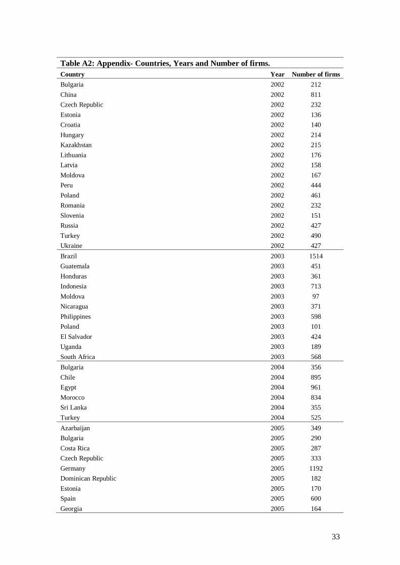
33
Table A2: Appendix- Countries, Years and Number of firms. Country Year Number of firms Bulgaria 2002 212 China 2002 811 Czech Republic 2002 232 Estonia 2002 136 Croatia 2002 140 Hungary 2002 214 Kazakhstan 2002 215 Lithuania 2002 176 Latvia 2002 158 Moldova 2002 167 Peru 2002 444 Poland 2002 461 Romania 2002 232 Slovenia 2002 151 Russia 2002 427 Turkey 2002 490 Ukraine 2002 427 Brazil 2003 1514 Guatemala 2003 451 Honduras 2003 361 Indonesia 2003 713 Moldova 2003 97 Nicaragua 2003 371 Philippines 2003 598 Poland 2003 101 El Salvador 2003 424 Uganda 2003 189 South Africa 2003 568 Bulgaria 2004 356 Chile 2004 895 Egypt 2004 961 Morocco 2004 834 Sri Lanka 2004 355 Turkey 2004 525 Azarbaijan 2005 349 Bulgaria 2005 290 Costa Rica 2005 287 Czech Republic 2005 333 Germany 2005 1192 Dominican Republic 2005 182 Estonia 2005 170 Spain 2005 600 Georgia 2005 164
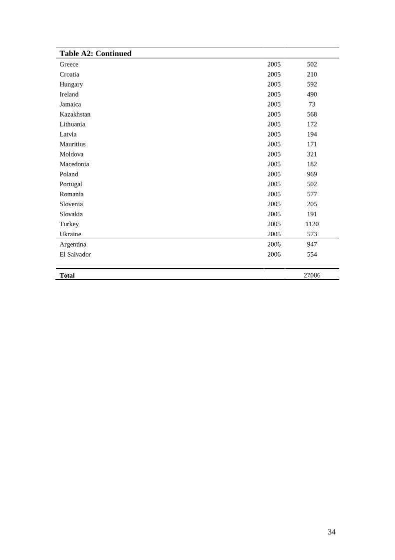
34
Table A2: Continued Greece 2005 502 Croatia 2005 210 Hungary 2005 592 Ireland 2005 490 Jamaica 2005 73 Kazakhstan 2005 568 Lithuania 2005 172 Latvia 2005 194 Mauritius 2005 171 Moldova 2005 321 Macedonia 2005 182 Poland 2005 969 Portugal 2005 502 Romania 2005 577 Slovenia 2005 205 Slovakia 2005 191 Turkey 2005 1120 Ukraine 2005 573 Argentina 2006 947 El Salvador 2006 554
Total 27086
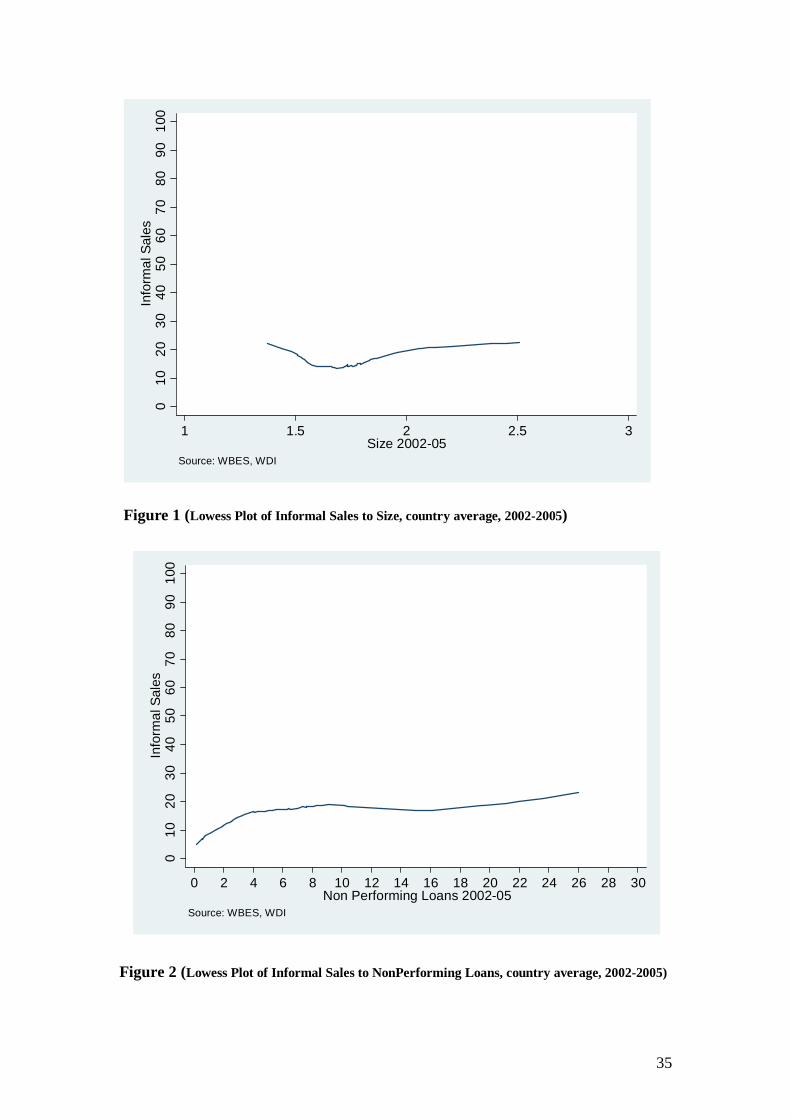
35
010
2030
4050
6070
8090
100
Info
rmal
Sal
es
1 1.5 2 2.5 3Size 2002-05
Source: WBES, WDI
Figure 1 (Lowess Plot of Informal Sales to Size, country average, 2002-2005)
Figure 2 (Lowess Plot of Informal Sales to NonPerforming Loans, country average, 2002-2005)
010
2030
4050
6070
8090
100
Info
rmal
Sal
es
0 2 4 6 8 10 12 14 16 18 20 22 24 26 28 30Non Performing Loans 2002-05
Source: WBES, WDI
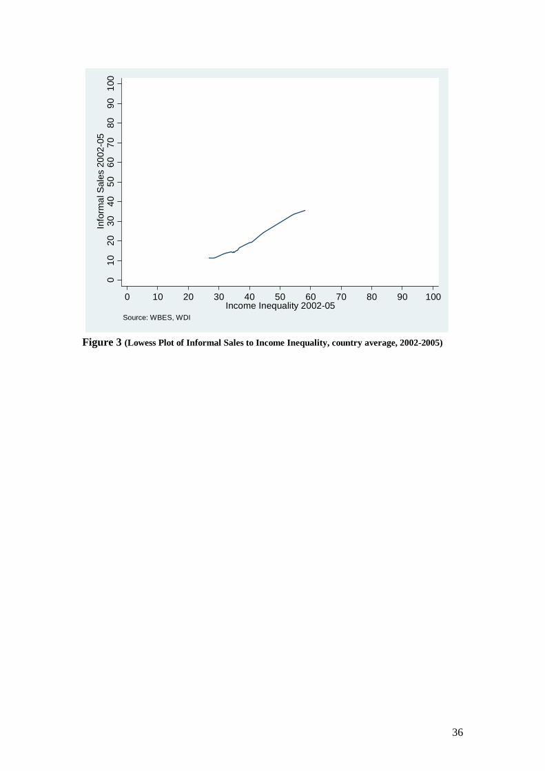
36
010
2030
4050
6070
8090
100
Info
rmal
Sal
es 2
002-
05
0 10 20 30 40 50 60 70 80 90 100Income Inequality 2002-05
Source: WBES, WDI
Figure 3 (Lowess Plot of Informal Sales to Income Inequality, country average, 2002-2005)