Informal Sanctions on Prosecutors and Defendants and the Disposition of Criminal Cases*

by

Andrew F. Daughety and Jennifer F. Reinganum**Department of Economics and Law School

Vanderbilt University

Original: May 2014This version: September 2014

* This paper was partly-written while visiting at the Paris Center for Law and Economics (Daughety) andthe University of Paris 2 (Reinganum); we especially thank Bruno Deffains for providing a supportiveresearch environment. We also thank Scott Baker, David Bjerk, Richard Boylan, Rosa Ferrer, FrancoiseForges, Luigi Franzoni, Nancy King, Kathryn Spier, Christopher Slobogin, and seminar participants at theUniversity of Bologna for comments and suggestions on an earlier version.

** andrew.f.daughety@vanderbilt.edu; jennifer.f.reinganum@vanderbilt.edu

Informal Sanctions on Prosecutors and Defendants and the Disposition of Criminal Cases

Abstract

We model the strategic interaction between a prosecutor and a defendant when informal sanctionsby outside observers (society) may be imposed on both the defendant and the prosecutor. Outside observersrationally use the disposition of the case (plea bargain, case drop, acquittal, or conviction) to impose thesesanctions, but also recognize that errors in the legal process (as well as hidden information) means they maymisclassify defendants and thereby erroneously impose sanctions on both defendants and prosecutors. If thirdparties prefer a legal system with minimal regret arising from classification errors, there is a uniqueequilibrium wherein the guilty defendant accepts the prosecutor’s proposed plea offer with positive (butfractional) probability, the innocent defendant rejects the proposed offer, and the prosecutor chooses to takeall defendants who reject the offer to trial.

We also consider the effect of increasing the informativeness of the jury’s decision by extending themodel to allow for a three-verdict outcome (not guilty, not proven, and guilty), sometimes referred to as the“Scottish” verdict. We find that: 1) guilty defendants are worse off, as plea bargains get tougher but therejection rate does not change; 2) innocent defendants are better off; 3) the prosecutor’s overall payoff goesup; and 4) the outside observers’ regret over possible misapplication of informal sanctions is reduced. Thusthe Scottish verdict is justice-improving when compared with the standard (two-outcome) verdict.

1. Introduction

All of us are familiar (if only from TV and the movies) with the fact that the criminal justice process

provides formal sanctions for convicted defendants. These formal sanctions generally take two forms:

incarceration (with the possibility of probation being used in some cases) and fines. In this paper we consider

a third form of sanction that arises from members of society who observe pieces of the process, draw

conclusions about the participants, and impose costs on the (perceived) offending party; we refer to these as

informal sanctions.

Formal sanctions are imposed on defendants who are judged guilty (that is, who have accepted a plea

bargain or were found guilty at trial),1 and informal sanctions on convicted defendants have a long history;

for example, defendants who have been judged guilty and served their sentences (or paid their fines) may find

it difficult to find housing and employment after release. Informal sanctions can also fall on defendants who

have only been arrested, and for whom any charges have been dropped. Only one-fourth of the states actually

prohibit the use of (pure) arrest information by employers when hiring (and the degree of enforcement is

unclear).2 Many states are silent on such matters (leaving the use of such information for hiring purposes

entirely at the discretion of employers), while the remainder have imposed some limitations. For example,

while Michigan prohibits employers asking about misdemeanor arrests that did not lead to conviction, no

restrictions are placed on asking about felony arrests that did not lead to conviction. There are a number of

firms that specialize in investigating job candidates’ past criminal records (which typically include arrests,

even if those arrests did not lead to conviction) and provide such services to employers. A recent online

1 We abstract from the use of formal sanctions for officials, but abuses such as prosecutorial misconduct can lead to formal sanctions. A fairly well-known example of prosecutorial misconduct involved Michael Nifong, the District Attorney for Durham County, NC, who was disbarredfor his actions in the 2006 Duke University lacrosse case prosecution; see NC State Bar v. Nifong (June 16, 2007). Nifong also was convicted ofcriminal contempt of court for lying to a judge and served one day in jail and paid a $500 fine; see Associated Press (2007).

2 The website Nolo.com provides state-level detail on the state and federal restrictions on the use by employers of information about arrestor conviction (www.nolo.com/legal-encyclopedia/state-laws-use-arrests-convictions-employment.html; accessed June 24, 2014). The EqualOpportunity Employment Commission provides guidance on what could constitute discriminatory hiring from a federal perspective, and only prohibitsblanket policies of not hiring those with arrest records. The EEOC reports survey results that 92% of responding employers use criminal or backgroundchecks on all or some of job candidates (http://www.eeoc.gov/laws/guidance/arrest_conviction.cfm#IIIA; accessed June 24, 2014).

2

development has been websites that publish booking photos (“mug shots”) that are part of the public record.3

Moreover, defendants who have been acquitted may be greeted with the suspicion that they were actually

guilty but the jury was unable to formally reach that conclusion.4

Informal sanctions may also be applied to officials in the system; for concreteness we specifically

focus on prosecutors, but others may also be subject to such sanctions. Some prosecutors may be viewed as

“soft on crime” or “not up to the task” in that cases against defendants believed to be guilty are dismissed,

or trials are lost. Other prosecutors may be viewed as abusing their position, railroading possibly innocent

defendants into accepting plea bargains, or by winning trials that seem unfair. Informal sanctions on the

prosecutor can affect her career concerns via election, appointment, promotion, or selection for judgeships,

or outside opportunities in private law firms and universities.

We view formal sanctions as operating via the existing judicial system while informal sanctions come

from members of society and reflect the beliefs of “outside observers.” Thus, both defendants and

prosecutors may experience losses due to informal sanctions applied by these same outside observers.

Importantly, we show how informal sanctions may affect (including limit) the use of formal sanctions.

More precisely, informal sanctions for the defendant involve outside observers drawing an inference

about how likely it is that the defendant is guilty, given the case disposition, and applying sanctions that are

proportional to this belief.5 These sanctions correspond to the outside observers withdrawing from further

interactions with the defendant; for instance, they may choose not to hire him for a job, or to avoid social

interactions with him, and so on. The proportional specification is a simple way to ensure that the defendant

3 See the discussion of the case of Dr. Janese Trimaldi, among others, in Segal (2013). Despite the fact that all charges against her weredropped, her booking photo (which is a public record) began to appear at online mug-shot sites. Segal estimates that there are over 80 such sites thatgenerally charge people to remove the images; he indicates that fees for removal of information tend to run between $30 and $400 and, since multiplesites may post the picture, the cost of eliminating this information from the web can be exorbitant.

4 One juror in the case against Casey Anthony (acquitted of murdering her two-year-old daughter), stated: “I did not say she was innocent;I just said there was not enough evidence. If you cannot prove what the crime was, you cannot determine what the punishment should be.” See Burke,et. al. (2011).

5 Other recent papers that incorporate payoffs (representing the assessments of third parties) that are proportional to inferred type includeBenabou and Tirole (2006), Daughety and Reinganum (2013), and Deffains and Fluet (2013).

3

suffers worse informal sanctions the higher is the outside observers’ belief in his guilt. Although these

informal sanctions are costly to the defendant, we assume that the outside observers do not bear any direct

cost of imposing them; for instance, they can simply hire, or interact socially with, someone else. As

suggested earlier, we also assume that the outside observers impose informal sanctions on the prosecutor, and

these too we take as being in proportion to their posterior belief that she has punished an innocent defendant

(through conviction at trial or through a plea-bargained conviction), or failed to punish a guilty defendant

(either through acquittal at trial or through dropping the case).

We find that informal sanctions will affect both the feasibility, and the willingness, of the prosecutor

to employ plea bargaining. In particular, the only type of equilibrium that can exist is a semi-separating one

wherein innocent defendants reject the plea offer,6 whereas guilty defendants mix between accepting and

rejecting the plea offer. Because the prosecutor has the option to drop the case, there must be a sufficient

fraction of guilty defendants among those that reject the plea offer in order to incentivize the prosecutor to

go to trial following rejection. Informal sanctions may restrict the feasibility of the equilibrium wherein at

least some defendants settle, as (in equilibrium) accepting the plea bargain results in a clear inference of guilt,

which results in the highest informal sanction against the defendant. If the informal sanction rate for the

defendant is too high, then it will not be possible to induce a defendant to accept a plea bargain. Similarly,

a prosecutor may prefer to take a case to trial rather than settling via a plea bargain if the informal sanction

rate on the defendant is too high, because the prosecutor has to discount the formal sanction (in the plea offer)

in order to induce the defendant to accept both the plea offer and the informal sanction that results when he

thereby reveals his guilt. The threshold informal sanction rate on the defendant increases in the informal

sanction rate on the prosecutor for punishing the innocent, as a higher informal sanction rate on the prosecutor

for punishing an innocent person makes trial (which can result in erroneous convictions) less attractive to the

6 Innocent defendants never accepting the equilibrium plea offer is a common characteristic of many of the economic analyses of pleabargaining. In reality, some innocent defendants do accept plea offers. The model’s prediction in this regard can be modified by incorporating asufficiently high degree of risk aversion or ambiguity aversion on the part of innocent defendants (that is, making defendants heterogeneous withregard to risk or uncertainty about the relevant probability distribution to use), but this is at a severe cost of making the model intractable and wouldobscure the interplay between informal sanctions and choices by defendants and prosecutors. We return to this topic near the end of the paper.

4

prosecutor. Thus, some informal sanctions work in opposition to others.

Because the equilibrium fraction of guilty defendants among those that reject the plea offer is co-

determined with the fraction that outside observers expect to reject the plea offer, there is a continuum of

semi-separating equilibria, indexed by this fraction. There is a smallest equilibrium fraction that is necessary

to incentivize the prosecutor to go to trial following a rejection (rather than dropping the case). We show that,

if outside observers prefer to minimize the extent of erroneously-imposed informal sanctions, then they prefer

the equilibrium wherein the smallest fraction of guilty defendants reject the plea offer. That is, they prefer

the equilibrium which entails the greatest amount of successful plea bargaining. This equilibrium involves

the lowest possible amount of “misclassification” because those that accept the plea offer are revealed to be

guilty types, and trial is the clearest possible signal of innocence (subject to the noise that is required to

incentivize the prosecutor to go to trial following a rejected plea offer).

Finally, we consider a legal system wherein the outside observers are able to acquire more

information from a jury as to the degree of guilt of the defendant. Specifically, we extend the model to

consider the “Scottish verdict” wherein the verdict allows for three outcomes: not guilty, not proven, and

guilty. The intermediate case, not proven, carries no formal sanctions (it is a form of acquittal); it represents

an outcome wherein jurors felt that the prosecution’s case against the defendant was insufficiently strong to

meet the high evidentiary standard needed in a criminal case (beyond a reasonable doubt), but also reflects

an unwillingness on the part of the jury to assert a belief that the defendant was not guilty. We show that this

finer resolution of the jury’s assessment leads to increased expected costs to a truly guilty defendant, lower

expected costs to a truly innocent defendant, and informal sanctions by outside observers that are more likely

to be deserved; altogether, these results suggest that the Scottish verdict is likely to be justice-enhancing

relative to the standard two-outcome (guilty/not guilty) verdict.

Related Literature

Landes (1971) provides a complete-information model wherein the prosecutor’s objective is to

maximize expected sentences obtained from a collection of defendants, subject to a resource constraint; the

5

potential for innocent defendants is not considered. Grossman and Katz (1983) and Reinganum (1988)

provide screening and signaling models, respectively, of plea bargaining wherein the prosecutor maximizes

a utility function that corresponds to social welfare. Grossman and Katz assume that the defendant knows

whether he is guilty or innocent; the prosecutor’s plea offer screens the defendant types so that the innocent

go to trial whereas the guilty accept the plea offer. Reinganum assumes that the defendant knows whether

he is guilty or innocent, but the prosecutor also has private information: she knows the actual likelihood of

conviction at trial. In this case, the plea offer signals the strength of the prosecutor’s case but it does not

screen the defendant types; both guilty and innocent defendants randomize between accepting the plea offer

and going to trial. Thus, the prosecutor goes to trial against a mixture of guilty and innocent defendants. In

both of these models, however, it is assumed that the prosecutor is committed to taking the case to trial

following a rejected plea offer; this means that even if the prosecutor knew the defendant was innocent, she

would pursue a conviction.

Absent this commitment to trial following a rejected plea, a putative equilibrium in which the guilty

accept the plea offer and the innocent reject it is undermined by the prosecutor’s desire to drop the case rather

than proceeding to trial against a defendant that (she now believes) is innocent. Franzoni (1999) and Baker

and Mezzetti (2001) explicitly incorporate a credibility constraint into a screening model, which requires that

a sufficiently high fraction of guilty defendants reject the plea offer.7 We also incorporate this kind of

credibility constraint; our model is closest in terms of the prosecutor’s payoff functions to that of Baker and

Mezzetti because in both models the prosecutor faces a risk of convicting an innocent defendant.8 However,

7 See Nalebuff (1987) for a screening model with a possibly-binding credibility constraint in the case of a civil suit. In Franzoni’s model,innocent defendants are never convicted, so the prosecutor simply maximizes the expected penalty imposed on the guilty less the cost of the effortshe expends to investigate prior to trial. However, if only innocent defendants reject the plea offer, then the prosecutor is unwilling to expend anyeffort on investigation; thus, equilibrium must involve some guilty defendants rejecting the plea offer as well.

8 In Baker and Mezzetti’s model, a prosecutor obtains a payoff of x (resp., - x) if a guilty (resp. innocent) defendant gets a sentence of x. The prosecutor obtains a payoff of zero if she frees an innocent defendant and - αx if she frees a guilty defendant. Finally, the prosecutor does nothave a cost of trial, but loses the amount c whenever she loses at trial (this is viewed as a reputational cost). Thus, in their model the prosecutor hasinternal concern for punishing the innocent and letting the guilty go free, and they obtain a unique semi-separating equilibrium. In our model thesesanctions are provided by the outside observers, and we obtain a continuum of semi-separating equilibria, and then use a selection criterion to obtaina unique (selected) equilibrium.

6

we will incorporate informal sanctions that fall on both the defendant and the prosecutor, depending on the

disposition of the case (e.g., convicted; acquitted; plea-bargained; or dropped).

The papers discussed thus far (as well as our paper) assume that the judge or jury makes its decision

based only on the evidence (“signal”) they observe in the course of the trial and the specified standard of

proof. That is, they follow their instructions rather than acting as rational Bayesian agents. Bjerk (2007)

provides a model in which the jury acts as a rational Bayesian agent, and this undermines an equilibrium

wherein the prosecutor screens defendant types perfectly. For if the prosecutor was expected to induce a

guilty plea from all of the guilty defendants, then the jury would rationally infer that those coming to trial

must be innocent, and the jury would acquit (but then the guilty would refuse to plead). The beliefs of the

jury are self-fulfilling and Bjerk finds that the model can have a continuum of equilibria, indexed by the

evidentiary threshold needed for the jury to convict the defendant.9

Our model also has a continuum of equilibria, but these are based on the (rational Bayesian) beliefs

of the outside observers, who impose informal sanctions on both the defendant and the prosecutor. As in

Franzoni (1999), Baker and Mezzetti (2001), and Bjerk (2007), our prosecutor will face a credibility

constraint in that she will have to ensure that there are enough guilty defendants among those that reject the

plea offer to rationalize her going to trial. Our multiple equilibria are indexed by the fraction of guilty

defendants among those that reject the plea offer (again, innocent defendants always reject the plea offer).

When outside observers believe that this fraction is high, then they impose high informal sanctions on

defendants following a trial, which allows the prosecutor to make a high plea offer that is rejected by a high

fraction of guilty defendants. On the other hand, if the outside observers believe that the fraction of guilty

defendants among those that reject the plea offer is low, then they impose low informal sanctions on

defendants following a trial, which constrains the prosecutor to make only a low plea offer that is rejected

9 Bjerk assumes that both the prosecutor and the jury maximize social welfare (given their respective beliefs and information), and trialsare costless. Our prosecutor’s objective increases in the sentences she obtains, but is also influenced by informal sanctions imposed by outsideobservers based on her perceived errors. Bjerk does not argue for a particular selection from among the equilibria he identifies. We argue for aparticular equilibrium to be selected based on the desire of outside observers to minimize the extent of informal sanctions that they impose in error.

7

by a low fraction of guilty defendants. Because the outside observers’ beliefs are based on coarse information

(i.e., the case disposition), they will sometimes impose informal sanctions on defendants and prosecutors that

are excessive or insufficient. We select among the equilibria in our model by positing a preference on the part

of the outside observers to minimize the expected regret due to erroneously-imposed informal sanctions.10

Finally, as indicated above, there are a number of different formulations for the prosecutor’s

objective, ranging from expected sentences to social welfare to a mixture of motivations. Prosecutors are in

an unusual position as they are supposed to represent society but they will clearly have personal preferences

and career concerns as well. The general issue of what it is that prosecutors are maximizing is important to

formulating models of plea bargaining. Glaeser, Kessler, and Piehl (2000), in a study of drug prosecutions

at the federal and state level, find that some federal prosecutors are motivated by reducing crime while others

appear to be primarily motivated by career concerns. Boylan and Long (2005) used data on young federal

prosecutors and found that those assistant U.S. attorneys in districts with very high private salaries were more

likely to take cases to trial, and viewed this as evidence that those positions for young prosecutors were

sought by individuals who wanted the trial experience, with an eye towards an eventual private-sector job.

Boylan (2005) expands on this by examining the careers of U.S. attorneys and finds that the length of prison

sentences obtained (but not conviction rates) is positively related to positive outcomes in their career paths.

Bandyopadhyay and McCannon (forthcoming), using data from North Carolina, find that prosecutors subject

to reelection pressure alter the mix of cases taken to trial (versus plea-bargained cases) so as to increase the

number of convictions at trial (this includes taking more weak cases to trial).11 McCannon (2013) uses data

from western New York and finds that cases taken by prosecutors during the six months before the election

10 Defendants also prefer this equilibrium. As we discuss later, despite the fact that outsiders incur no cost for imposing sanctions, analternative basis for choosing this equilibrium is that outsiders under a veil of ignorance (so that they recognize that they may be defendants one day)would prefer the same equilibrium as that which minimizes expected regret.

11 Gordon and Huber (2002) argue that voters concerned with prosecutorial power (including those worried about conviction of innocents)and who desire imposing accountability on prosecutors should follow a strategy of reelecting prosecutors who pursue cases to trial and obtainconvictions. In their model the prosecutor can, with effort, observe the true guilt or innocence of the defendant and go to trial with “unimpeachableevidence” so that truly innocent cases are dropped.

8

(and then later appealed) are more likely to be reversed by the appellate court: it appears that the desire to

influence the election leads to more wrongful convictions.

In our model prosecutors maximize the expected sentence (that is, statutory length times the

likelihood of conviction), minus the cost of trial, and minus the expected informal sanctions from outside

observers arising from convicting the innocent or not convicting the guilty.12 Thus, our prosecutor’s objective

reflects career concerns that are modeled as being a function of statutory sentence length, likelihood of

conviction, and the possibility of informal sanctions from outside observers.

Plan of the Paper

In Section 2, we provide the notation and formal model. In Section 3, we describe the equilibria of

the model (the equilibrium concept will be Perfect Bayesian equilibrium), and a rationale for selecting among

them. We then discuss some important comparative statics due to the informal sanctions on the defendant

and on the prosecutor. Section 4 extends the model to the Scottish verdict and shows that this refinement

enhances justice. In Section 5, we provide a summary and some additional discussion, and we raise some

possible extensions. A few of the most salient technical issues are included in the Appendix while a

Technical Appendix13 contains the full details of the analysis.

2. Modeling Preliminaries

Description of the Game

Our game commences after the police arrest the defendant on suspicion of committing a specific

crime. The defendant, D, will be taken to be male, and the prosecutor, P, female. The exogenous parameters

of the game include the sentence upon conviction (Sc), the evidentiary criterion used by the jury for

12 One might question whether it is fair to place all the weight of getting it right on the prosecutor when there is incomplete informationabout the defendant and imperfect information about the evidence and the jury. We would argue that it is the prosecutor who chooses to make an offer(or not), to drop a case or to pursue the case to trial, and that the foregoing empirical studies, in toto, generally support a model focused around careerconcerns that reflect social preferences regarding criminality and the use of prosecutorial power.

13 Available at http://www.vanderbilt.edu/econ/faculty/Daughety/DR-InformalSanctionsandCaseDispositions-TechApp.pdf

9

conviction (γc), and the cost of trial for each agent (kP for P and kD for D). More detail on the notation (and

the informal sanctions, which also have exogenously-determined elements) will be provided as we progress,

but a basic notational convention will be that outcomes or actions appear as subscripts while “ownership” –

that is, which agent is affected by the variable or parameter of interest – is indicated by a superscript.

There are five stages in the game:

Stage 1: Nature (N) draws D’s type, denoted by t, and this is revealed to D only.

Stage 2: P makes a plea bargain offer of Sb > 0 (since P is the only agent who can make such offers

in our analysis, ownership is implied).

Stage 3: D chooses whether to accept (A) or reject (R) the plea bargain offer; if he accepts the offer

(outcome b), the game ends and payoffs (πbP and πb

D) are obtained.

Stage 4: If D has chosen R, then P now chooses whether to drop the case (outcome d) or pursue it

to trial (action T). A case that is dropped means that P and D obtain payoffs πdP and πd

D,

respectively.

Stage 5: If the case goes to trial (T), then Nature (N) draws the evidence of guilt, e, and the jury (J)

uses the rule that if e > γc, then the outcome is conviction (c), while otherwise the outcome

is acquittal (a). In the case of conviction P and D obtain πcP and πc

D, respectively, while in the

case of acquittal P and D obtain πaP and πa

D, respectively.

Figure 1 below illustrates the sequence of actions and outcomes in the game (the “fans” indicate that

the specified variable can take on a continuum of values); we have not indicated information sets so as to

make the diagram more readable.

Let t 0 {I, G} denote D’s privately-known type (Innocent or Guilty), and let λ > 0 denote the fraction

of innocent Ds; that is λ = Pr{t = I}, the probability that a D at the left end of Figure 1 is innocent of the crime

for which he was arrested. This parameter reflects some initial level of evidence gathered by the police. As

indicated above, no further evidence is available until P and D go to trial, in which case a draw of evidence

of guilt, e 0 [0, 1], occurs; this draw is influenced by the underlying type for D and is observed only by the

10

jury. The jury is instructed to convict if its evidence signal exceeds a threshold (γc) and to otherwise acquit

the defendant. We denote the distribution of evidence (given D’s type) as F(e | t), which we assume is

continuous in e. Since for any evidentiary standard for conviction, γc, the jury (J) will choose outcome a

when e < γc, then for either type t, F(γc | t) is the probability that D is acquitted and 1 - F(γc | t) is the

probability that D is convicted. This motivates the assumption that at any level of evidence e, the probability

of acquittal for an innocent D is higher than that for a guilty D:

F(e | I) > F(e | G) for all e.

Finally, to aid readability in writing out payoffs, let Ft denote F(γc | t), for t = I, G, so our assumption implies

that FI > FG.

The sentences Sc and Sb are formal sanctions. Informal sanctions are penalties imposed by outside

observers on both defendants and prosecutors; to reduce the verbiage, let Θ denote the outside observer(s).14

Informal sanctions are based on Θ’s beliefs, which are contingent on the case disposition (a, b, c, or d). We

assume that these informal sanctions are proportional to the observers’ beliefs, which depend upon the

inferred type of defendant and the observed outcome of the legal process.15 More precisely, these beliefs

14 Since we will not be accounting for any heterogeneity among the outside observers, we will refer to both singular possessive and pluralpossessive Θ (e.g., we will refer to Θ’s and Θs’ beliefs) interchangeably. Outside observer beliefs will always be denoted by μ, so ownership of suchbeliefs will be obvious and therefore superscripting them with a Θ is unnecessary.

15 For simplicity, we assume that the outside observers always observe the case disposition. However, it is trivial to allow this to occuronly with positive probability. Probabilistic observation would simply re-scale the informal sanction rates by pre-multiplying these rates by theprobability that the observers actually do observe the case disposition.

11

represent Θ’s posterior probability that the defendant is type t, given the case disposition was y, and are

denoted μ(t | y), where t = I, G and y = a, b, c, d. Note that this also means that Θ cannot directly observe the

plea offer, Sb, the levels of P’s and D’s payoffs, or the evidence draw e.16

Informal sanctions imposed on D are of the form rDμ(G | y), where rD > 0 is an exogenous parameter.17

That is, given any case disposition, Θ assesses the posterior likelihood that D is guilty, and then imposes

informal sanctions at the rate rD. These informal sanctions, which are increasing in the posterior assessment

of guilt, reflect the fact that Θs may be future trading partners (broadly-construed) who decline to trade with

the defendant; we assume that the observers themselves do not suffer a direct cost of imposing these sanctions

(though we will later assume that they prefer a society that minimizes the extent of erroneously-imposed

informal sanctions).

As indicated earlier, Θs also impose informal sanctions on P, reflecting the notion that errors occur

within the legal process; informal sanctions imposed on the prosecutor arise when there is a belief that

prosecutors should be blamed for such perceived errors; for instance, a guilty defendant may be acquitted or

the case may be dropped. In these instances, P has allowed a guilty D to escape punishment. The associated

informal sanctions are given by rPGμ(G | y), for y 0 {a, d}. On the other hand, an innocent defendant can be

convicted or may accept a plea bargain. In these instances, the prosecutor has punished an innocent

defendant. The associated informal sanctions are given by rPIμ(I | y), for y 0 {b, c}. We assume that rP

I and

rPG are non-negative. While not needed in the model, a natural assumption would be that the sanction rate for

the prosecutor is higher when an innocent defendant is punished than when a guilty defendant is not punished;

that is, rPI > rP

G.18

16 It is very plausible that Θ would not observe a rejected plea offer. Our analysis assumes that Θ does not observe the plea bargain offerSb, even if D accepts the bargain and the fact of that acceptance is observed. We speculate that, due to the structure of the game and the fact that thereare only two types of D, observing Sb if D accepts the offer would not affect Θ’s out-of-equilibrium beliefs, but we leave this as an item for futureresearch; see our discussion of transparency in the last section.

17 In general we think of this rate as positive, but it could be negative (which the model accommodates), such as might hold if D was agang member desiring “street cred” and the relevant set of outside observers was restricted to gang members and friends. Moreover, rD may differfrom one crime to another; a heinous crime is likely to have a higher value of this parameter than a petty crime.

18 As with rD, rPI and rP

G may vary with the crime in question.

12

D’s Payoffs

We are interested in non-cooperative solutions for the game that exhibit sequential rationality by G,

I, P and Θ, so we will first develop payoff functions starting from the outcomes (a, b, c, and d). Since trial

ends in conviction or acquittal, D’s payoffs on the right-hand-side of Figure 1 can be written as (note that D

chooses actions so as to minimize his total expected payoff):

πcD = Sc + kD + rDμ(G | c); (1a)

and πaD = kD + rDμ(G | a). (1b)

That is, going to trial costs D the amount kD. Conviction results in the formal sanction Sc plus the informal

sanction rDμ(G | c); since I-types may have been convicted (the evidence draw for an I-type could,

conceivably, result in conviction), Θ recognizes that conviction is not a guarantee of guilt, so μ(G | c) will

be less than one. Similarly, acquittal generally does not imply innocence, so Θ’s belief μ(G | a) will be

positive and D will bear both the cost of trial and the informal sanction rDμ(G | a).

We can write D’s expected loss from going to trial (given his type t) as the weighted combination

of the elements in equations (1a) and (1b), where the weights reflect the likely outcome at trial:

πTD(t) = Sc(1 - Ft) + kD + rDμ(G | c)(1 - Ft) + rDμ(G | a)Ft, t 0 {I, G}. (2)

For instance, if t = I, then if D goes to trial, he expects to be convicted (outcome c) with probability 1 - FI,

in which case he will receive the formal sanction Sc and the informal sanction rDμ(G | c). He expects to be

acquitted (outcome a) with probability FI, in which case he will receive no formal sanction but Θ still believes

there is a chance D is guilty despite his acquittal, and imposes the informal sanction rDμ(G | a). Also note that

D pays his trial costs kD regardless of the trial outcome. The following result is shown in the Technical

Appendix.

Remark 1: πTD(I) < πT

D(G).

That is, a D of type I has a lower expected loss from trial than does a D of type G. This result follows from:

1) the linear structure of πTD(t) and 2) the fact that FI > FG. Remark 1 is important in that it suggests that the

equilibrium might involve full screening (wherein, say, P makes an offer that only G-types accept and I-types

13

reject), or partial screening (wherein, say, P makes an offer that all of one type reject, and that some of the

other type reject); that is, properly-constructed offers in the plea bargaining stage may yield information about

D’s type. We return to this in Section 3 in our discussion of the equilibria of the game.

If P offers a plea bargain of Sb, then D can choose to accept (A) or reject (R) the offer. D’s payoff

from accepting a plea bargain of Sb is:

πbD = Sb + rDμ(G | b); (3)

that is, he receives the formal sanction Sb plus the informal sanction that observers impose because, having

accepted the plea offer (outcome b), they believe that he is guilty with probability μ(G | b).

Similarly, D’s payoff if P drops the case is:

πdD = rDμ(G | d), (4)

which reflects Θ’s beliefs that D might have been guilty.

Since P may mix between going to trial and dropping the case following a rejection of the plea offer

by D, let ρP denote the probability that P takes the case to trial following rejection by D. Combining

equations (2) and (4), weighted by the probability that P takes the case to trial, yields D’s expected payoff

following rejection (given his type) as:

πRD(t) = ρPπT

D(t) + (1 - ρP)πdD. (5)

P’s Payoffs

Again, starting at the right of Figure 1, since trial ends in conviction or acquittal, P’s payoffs on the

right-hand-side of Figure 1 can be written as (note that P chooses actions so as to maximize her total expected

payoff):

πcP = Sc - k

P - rPIμ(I | c); (6a)

πaP = - (kP + rP

Gμ(G | a)). (6b)

Next we obtain P’s expected payoff from going to trial; this turns out to be somewhat more

complicated than D’s corresponding payoff because P and Θ have different amounts of information on which

to form beliefs. When the prosecutor makes the plea offer Sb, she does not know whether the defendant is

14

guilty or innocent, so D’s decision to accept or reject the offer will affect the prosecutor’s posterior belief that

he is guilty. The prosecutor’s beliefs may differ from those of the observer because she observes the plea

offer, whereas the observer observes only the disposition of the case. To capture this, let ν(G | R) (resp.,

ν(G | A)) denote the prosecutor’s posterior probability that the defendant is guilty,19 given that he rejected

(resp., accepted) the plea offer Sb. Of course, in equilibrium, P’s beliefs and Θ’s beliefs must be the same

(and must be correct).

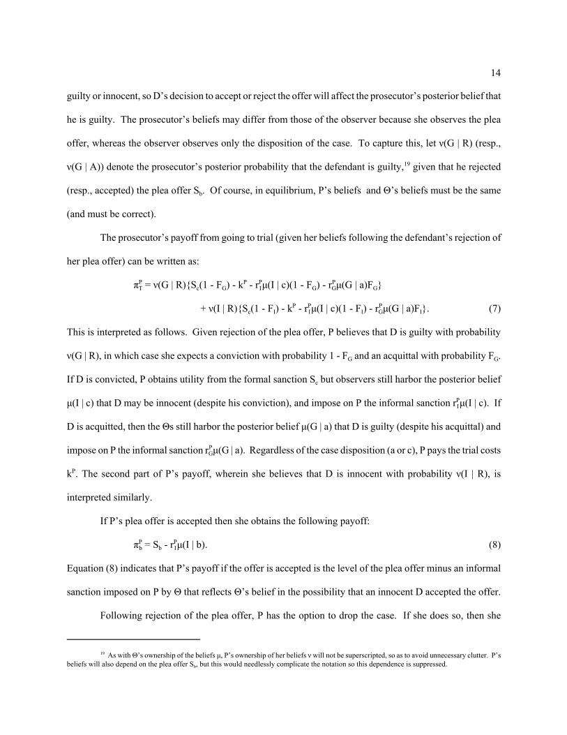
The prosecutor’s payoff from going to trial (given her beliefs following the defendant’s rejection of

her plea offer) can be written as:

πTP = ν(G | R){Sc(1 - FG) - kP - rP

Iμ(I | c)(1 - FG) - rPGμ(G | a)FG}

+ ν(I | R){Sc(1 - FI) - kP - rP

Iμ(I | c)(1 - FI) - rPGμ(G | a)FI}. (7)

This is interpreted as follows. Given rejection of the plea offer, P believes that D is guilty with probability

ν(G | R), in which case she expects a conviction with probability 1 - FG and an acquittal with probability FG.

If D is convicted, P obtains utility from the formal sanction Sc but observers still harbor the posterior belief

μ(I | c) that D may be innocent (despite his conviction), and impose on P the informal sanction rPIμ(I | c). If

D is acquitted, then the Θs still harbor the posterior belief μ(G | a) that D is guilty (despite his acquittal) and

impose on P the informal sanction rPGμ(G | a). Regardless of the case disposition (a or c), P pays the trial costs

kP. The second part of P’s payoff, wherein she believes that D is innocent with probability ν(I | R), is

interpreted similarly.

If P’s plea offer is accepted then she obtains the following payoff:

πbP = Sb - r

PIμ(I | b). (8)

Equation (8) indicates that P’s payoff if the offer is accepted is the level of the plea offer minus an informal

sanction imposed on P by Θ that reflects Θ’s belief in the possibility that an innocent D accepted the offer.

Following rejection of the plea offer, P has the option to drop the case. If she does so, then she

19 As with Θ’s ownership of the beliefs μ, P’s ownership of her beliefs ν will not be superscripted, so as to avoid unnecessary clutter. P’sbeliefs will also depend on the plea offer Sb, but this would needlessly complicate the notation so this dependence is suppressed.

15

receives no payoff from formal sanctions, but she receives an informal sanction from Θ, who believes with

probability μ(G | d) that D is guilty, so by dropping the case P let a guilty defendant go free. Thus, P’s payoff

from dropping the case is simply:

πdP = – rP

Gμ(G | d). (9)

As earlier, since P may mix between dropping the case and going to trial, P’s expected payoff

following a rejection by D is given by:

πRP = ρPπT

P + (1 - ρP)πdP. (10)

3. Results

In this section we provide the main results; a sketch of the derivation is in the Appendix while the

Technical Appendix contains the complete analysis. We start by providing notation for the strategies for each

type of D and for P, for Θ’s conjectures about these strategies, and two restrictions on the parameter space

that reflect sensible behavior by P. We then describe the game’s equilibria and the reasons for selecting a

specific equilibrium.

First, we denote a strategy profile as a four-tuple of strategies, one for P in Stage 2, one for each type

of D in Stage 3, and one for P in Stage 4:

(Sb, ρGD, ρ I

D, ρP) 0 [0, 4)×[0, 1]×[0, 1]×[0, 1],

where Sb is the plea offer made by P; ρGD is the probability a D of type G rejects the plea bargain offer; ρ I

D is

the probability a D of type I rejects the plea bargain offer; and ρP is the probability that P goes to trial against

a D who rejected the offer (rather than dropping the case). Thus, suppressing the plea offer for now, a

candidate equilibrium wherein both types of D always reject the offer Sb and P always goes to trial is (1, 1, 1).

Notice that P has conjectures about what types of D will choose to reject the offer. D has conjectures about

what P will do, conditional on D’s action and, while Θ cannot observe P’s and D’s actions, Θ has conjectures

about what P will do and about what the types of D will do. All conjectures must be correct in equilibrium,

16

but since P’s and D’s conjectures are not the primary focus of the paper (and are pretty standard) we do not

generate additional notation for these conjectures.

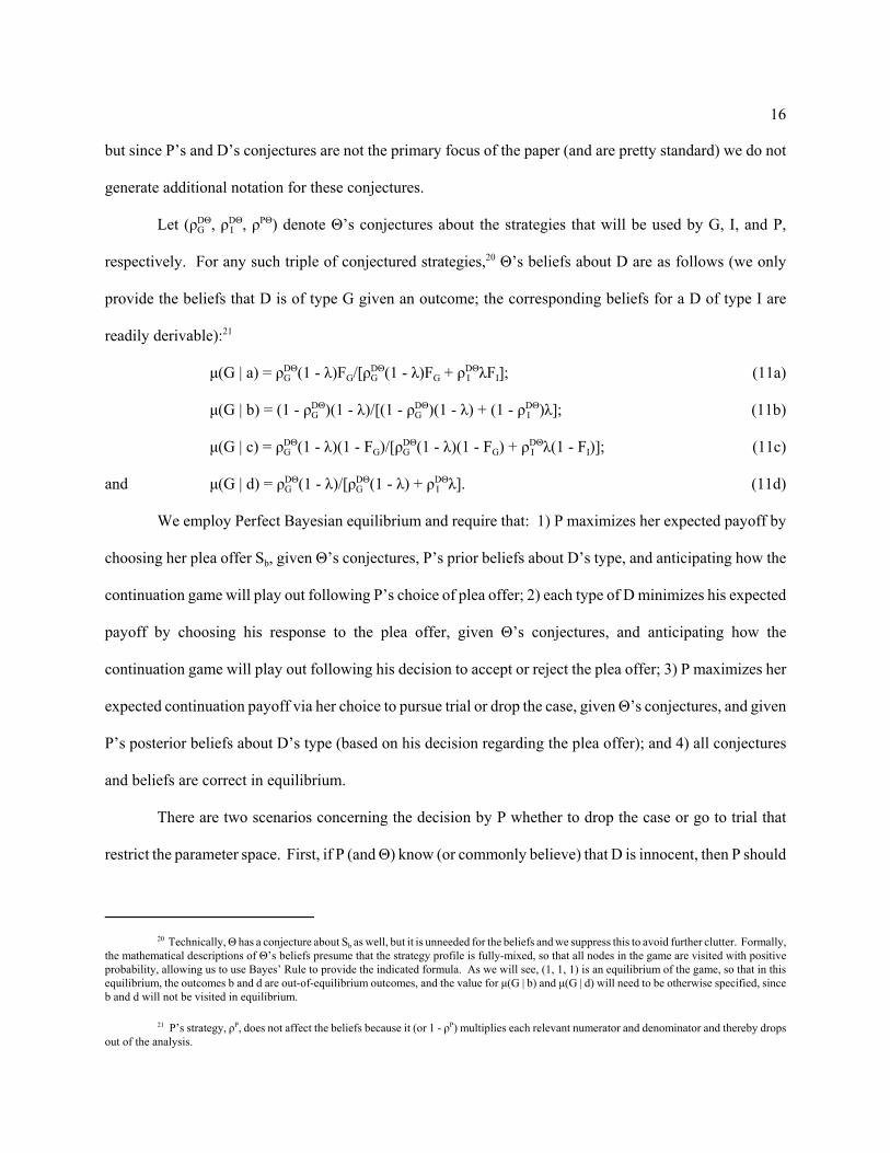
Let (ρGDΘ, ρ I

DΘ, ρPΘ) denote Θ’s conjectures about the strategies that will be used by G, I, and P,

respectively. For any such triple of conjectured strategies,20 Θ’s beliefs about D are as follows (we only

provide the beliefs that D is of type G given an outcome; the corresponding beliefs for a D of type I are

readily derivable):21

μ(G | a) = ρGDΘ(1 - λ)FG/[ρG

DΘ(1 - λ)FG + ρ IDΘλFI]; (11a)

μ(G | b) = (1 - ρGDΘ)(1 - λ)/[(1 - ρG

DΘ)(1 - λ) + (1 - ρ IDΘ)λ]; (11b)

μ(G | c) = ρGDΘ(1 - λ)(1 - FG)/[ρG

DΘ(1 - λ)(1 - FG) + ρ IDΘλ(1 - FI)]; (11c)

and μ(G | d) = ρGDΘ(1 - λ)/[ρG

DΘ(1 - λ) + ρ IDΘλ]. (11d)

We employ Perfect Bayesian equilibrium and require that: 1) P maximizes her expected payoff by

choosing her plea offer Sb, given Θ’s conjectures, P’s prior beliefs about D’s type, and anticipating how the

continuation game will play out following P’s choice of plea offer; 2) each type of D minimizes his expected

payoff by choosing his response to the plea offer, given Θ’s conjectures, and anticipating how the

continuation game will play out following his decision to accept or reject the plea offer; 3) P maximizes her

expected continuation payoff via her choice to pursue trial or drop the case, given Θ’s conjectures, and given

P’s posterior beliefs about D’s type (based on his decision regarding the plea offer); and 4) all conjectures

and beliefs are correct in equilibrium.

There are two scenarios concerning the decision by P whether to drop the case or go to trial that

restrict the parameter space. First, if P (and Θ) know (or commonly believe) that D is innocent, then P should

20 Technically, Θ has a conjecture about Sb as well, but it is unneeded for the beliefs and we suppress this to avoid further clutter. Formally,the mathematical descriptions of Θ’s beliefs presume that the strategy profile is fully-mixed, so that all nodes in the game are visited with positiveprobability, allowing us to use Bayes’ Rule to provide the indicated formula. As we will see, (1, 1, 1) is an equilibrium of the game, so that in thisequilibrium, the outcomes b and d are out-of-equilibrium outcomes, and the value for μ(G | b) and μ(G | d) will need to be otherwise specified, sinceb and d will not be visited in equilibrium.

21 P’s strategy, ρP, does not affect the beliefs because it (or 1 - ρP) multiplies each relevant numerator and denominator and thereby dropsout of the analysis.

17

prefer dropping the case to going to trial. Second, imagine that both types of D were expected to reject P’s

offer. Then P’s (and Θ’s) posterior beliefs about the types would be the same as the prior beliefs (that

Pr{t = I} = λ); this would also be true if there was no stage involving P making a plea bargain offer. In this

scenario, P should prefer trial over dropping the case; this will be true if the police arrest process procedure

is sufficiently effective at discriminating between guilty and innocent persons; that is, if λ, the prior

probability that D is of type I, is not “too large.”22 These two scenarios imply the following maintained

restrictions.

Maintained Restriction 1 (hereafter, MR1): If P and Θ know (or commonly believe) that D is of type

I, P should prefer to drop the case. Formally, this means that πTP < πd

P under the specified

beliefs, which reduces to: (Sc - rPI)(1 - FI) - k

P < 0. Notice that this can hold even if kP is

zero, as long as rPI exceeds Sc; lower values of rP

I are still feasible if kP is sufficiently positive.

Maintained Restriction 2 (hereafter, MR2): If P and Θ know (or commonly believe) that the fraction

of type G among those that reject the plea offer is the same as the prior, then P should prefer

to take the case to trial rather than dropping it. Formally, this restriction reduces to:

(1 - λ)[(Sc + rPG)(1 - FG) - kP] + λ[(Sc - r

PI)(1 - FI) - k

P] > 0.

Note that the second term in brackets in MR2 is negative by MR1, so the above condition is an upper

bound on λ (the arrest process is sufficiently effective). Moreover, MR1 implies that the first term in brackets

in MR2, which represents the difference in the value of going to trial versus dropping the case against a D

that is known (or commonly believed) to be type G, is positive. Basically, P prefers to drop rather than try

cases against known innocent types, and prefers to try rather than drop cases against known guilty types;

moreover, she still prefers to try rather than drop against the prior mixture of defendant types.

Using these natural parameter restrictions, we find that the only23 equilibria of the game involve the

22 Essentially, this is the reason for requiring probable cause for an arrest (i.e., there is a reasonable basis to believe a potential D committeda specific crime).

23 Alternative candidates for equilibria, such as fully-separating or fully-pooling candidates, or candidates involving type I accepting aplea offer, cannot be equilibria; see the Technical Appendix for details.

18

D of type I always rejecting the equilibrium plea offer (so, hereafter, ρ ID = 1), the D of type G rejecting the

equilibrium plea offer with a positive probability ρGD, and P never dropping a case when D rejects an offer.

We provide a sketch of the proof of the following Proposition, which formalizes the description of the game’s

continuum of equilibria, in the Appendix (the complete proof is in the Technical Appendix). To simplify the

exposition of the Proposition, 1) let πTD(G; ρG

D) be πTD(G), as specified in equation (4), with Θ’s beliefs

evaluated at ρGD and ρ I

D = 1; and 2) define ρGD0 as the (unique) solution to the condition that πT

P = πdP, where both

of these expressions have Θ’s beliefs and P’s beliefs evaluated at ρGD0 (the specific value of ρG

D0 appears in

equation (14) below).24

Proposition 1: If rD is not “too large” then there is a unique family of Perfect Bayesian equilibria for

the game summarized by the four-tuple (Sb(ρGD), ρG

D, 1, 1), with ρGD 0 [ρG

D0, 1], ρGD0 a positive fraction.

For each ρGD, P’s equilibrium plea offer is Sb(ρG

D) = πTD(G; ρG

D) - rD.

Note the following:

1) Both the D of type I and P use pure strategies in equilibrium: all Ds who are innocent reject P’s

equilibrium offer, and the equilibrium involves a sufficient fraction of Ds who are guilty that

also reject the plea offer, so that P will not choose to drop any case.25

2) One member of this family of equilibria is (Sb(1), 1, 1, 1) wherein ρGD = 1, in which case all Ds are

rejecting P’s offer, meaning that P’s (and Θ’s) beliefs about the types that chose R is the

prior, so (by MR2) P goes to trial against all Ds.26

3) The smallest ρGD-value (ρG

D0) in the family of equilibria is in (0, 1), so in almost all of the equilibria

in the Proposition, G-types accept the plea offer with positive probability. From the

24 Beliefs for Θ are given by equations 11(a-d), evaluated at arbitrary ρGD and ρ I

D = 1; beliefs for P are given byν(G | R) = ρG

D(1 - λ)/[ρGD(1 - λ) + λ], as ρG

D of the G-types and all of the I-types are expected to reject the plea offer.

25 Out-of-equilibrium beliefs for Θ following an unexpected dropped case are μ(G | d) = ρGD(1 - λ)/[ρG

D(1 - λ) + λ]; since ρGD of the G-types

and all of the I-types are expected to reject the plea offer, Θ interprets the unexpected dropped case as an error on the part of P.

26 Now we also need an out-of-equilibrium belief for Θ’s observation of outcome b; that belief would be that the type is G, since G doesworse at trial than does I, so observing b should be associated with t = G: μ(G | b) = 1. Alternatively put, I is willing to reject the plea offer for astrictly larger probability of subsequently going to trial than is G, so selection of the “safe” option (accept) is attributed to G. This argument is anapplication of the Cho and Kreps (1987) refinement D1.

19

perspective of Θ, since I-types always reject the offer, this means that μ(G | b) is one: a D

who accepts the offer incurs the full sanction rD from Θ.

Limits on Informal Sanctions

What do we mean by the qualifier in Proposition 1 “If rD is not ‘too large’”? Consider those

equilibria wherein ρGD 0 [ρG

D0, 1); that is, G-types accept P’s offer with positive probability. In order for this

to occur, P must: 1) be choosing Sb from a non-empty set and 2) not wish to defect by making a very high

offer to D so as to make D reject the offer for sure. Notice that the Proposition indicates that Sb(ρGD) =

πTD(G; ρG

D) - rD, so that the set of feasible Sb-values capable of inducing some acceptance is [0, πTD(G; ρG

D) - rD].

Hence, in order to have a non-empty feasible set for Sb, it must be that rD < πTD(G; ρG

D). Substituting into this

inequality yields our first condition restricting the level of informal sanctions, Condition 1 (see the Technical

Appendix for more detail):

Condition 1 (feasibility). In order for P to be able to induce a D of type G to accept a plea offer, it

must be that: rD < [Sc(1 - FG) + kD]/[1 - μ(G | c)(1 - FG) - μ(G | a)FG].

Multiplying through both sides of the above inequality by the expression in the denominator on the

right, the resulting expression rD[1 - μ(G | c;)(1 - FG) - μ(G | a; )FG] is the increment in informal sanctions that

the D of type G suffers by accepting a plea (which only a true G is expected to do) rather than going to trial

(where there are trial costs plus a chance of conviction and a chance of acquittal, with corresponding informal

sanctions), which is the resulting term now on the right (i.e., Sc(1 - FG) + kD). If there were no positive

informal sanctions for D, then Condition 1 would be satisfied automatically.

Thus, positive informal sanctions on D constrain P’s ability to settle cases via plea bargain. Were

rD to violate Condition 1, the feasible set of plea offers that P could optimize over would be empty, resulting

in evisceration of plea bargaining. This means that beliefs by P (and Θ) would be given by the prior, and

according to MR2, P would always go to trial.

The second issue of concern (item (2) in the first paragraph of this sub-section) is that the informal

sanctions may result in P defecting from her part of the equilibrium by making a larger plea offer that

20

provokes both types to reject. This could occur if, despite the presence of informal sanctions in P’s expected

payoff from trial, Sb(ρGD) = πT

D(G; ρGD) - rD was less than what P could obtain by driving those D’s that would

have otherwise settled to trial. In the Technical Appendix we derive Condition 2 as the restriction that

eliminates this incentive for defection by P.27

Condition 2 (no defection). For P to find it preferable to settle with a D of type G rather than

provoking trial (holding Θ’s beliefs fixed at the equilibrium ρGD), it must be that:

rD < [kP + kD + rPIμ(I | c)(1 - FG) + rP

Gμ(G | a)FG]/[1 - μ(G | c)(1 - FG) - μ(G | a)FG].

The point of displaying this condition is that while rD again appears on the left (and the denominators of the

expressions in the two Conditions are the same), the informal sanctions on P, at rates rPI and rP

G, contribute to

the magnitude of the right-hand-side, and therefore alsso affect the ability to conclude a successful plea

bargain.

Finally, P could also defect by dropping all cases; again, this would not change the observers’ beliefs,

but we need to verify that P prefers the hypothesized equilibrium outcome to what she would get by defecting

to dropping all cases. Condition 1, however, is sufficient to imply this preference. To see why, notice that

in the hypothesized equilibrium (Sb(ρGD), ρG

D, 1, 1), P’s payoff is:

(1 - ρGD)(1 - λ)[πT

D(G; ρGD) - rD] + (ρG

D(1 - λ) + λ)πTP(ρG

D).

It is straightforward to show that P is indifferent between trying and dropping the case for ρGD = ρG

D0 (and

strictly prefers trying to dropping for ρGD > ρG

D0; see the Technical Appendix). Then Condition 1 implies that

the settlement offer Sb(ρGD) = πT

D(G; ρGD) - rD is non-negative, whereas P’s payoff from dropping the case is

- rPGμ(G | d), which is strictly negative. Thus, P strictly prefers the outcome involving some plea bargaining

to defecting to dropping all cases.

Since P prefers to settle via plea bargain rather than going to trial against type G when Condition 2

holds, why can’t P offer a slightly lower plea offer than Sb(ρGD) = πT

D(G; ρGD) - rD and induce type G to accept

27 Condition 2 is not necessary in the (1, 1, 1) equilibrium (i.e., when all types reject P’s offer).

21

with probability 1? The reason is that P needs to maintain her own incentives to go to trial following

rejection. If P were to offer a slightly lower plea offer designed to induce type G to accept for sure, then G

should expect the case to be dropped following rejection (since P’s subsequent beliefs should be that every

rejection is coming from a D of type I). This will cause type G to reject this offer, despite its apparent allure.

Consequently, P cannot gain by deviating to a lower plea offer.28

Selecting an Equilibrium

Proposition 1 characterizes the nature of the equilibria for the game, but we are still left with a

continuum of equilibria. We now propose a basis to select a unique member of that family, namely

(Sb(ρGD0),ρG

D0, 1, 1), which is the equilibrium with the highest fraction of G-types that choose to accept the plea

bargain.

Notice that Θ’s beliefs punish I-types by lumping them in with G-types. For example, rDμ(G | c) is

the sanction for a D that is convicted, whether he is truly guilty or innocent; if Θ knew that D was a wrongly-

convicted I, then one would expect the sanction to be (at worst) zero. Θ erroneously punishes an I, based on

observing a conviction, with probability λ(1 - FI), so the misclassification cost is λ(1 - FI)rDμ(G | c). Similarly,

if P obtains a conviction against D, then she will suffer an informal sanction based on Θ’s beliefs that the

convicted D might be innocent, in the amount of rPIμ(I | c). But if Θ knew that D was a wrongly-convicted

I, then the appropriate informal sanction for P would be rPI. Thus the outside observer’s misclassification cost

is λ(1 - FI)[rPI - r

PIμ(I | c)].

In the Appendix we assume that these costs are additive and we provide an overall “ expected regret”

measure, denoted as R(ρGD), which is shown to reduce to the following expression:

R(ρGD) = (rD + rP

I){λ(1 - FI)μ(G | c) + ρGD(1 - λ)(1 - FG)μ(I | c)}

+ (rD + rPG){λFIμ(G | a) + ρG

D(1 - λ)FGμ(I | a)}. (13)

28 For the equilibrium at ρGD = ρG

D0, there is actually a continuation equilibrium following the out-of-equilibrium plea offer Sb < Sb(ρGD)

wherein type G mixes between accepting and rejecting the plea offer with probability ρGD0 and P mixes between taking the case to trial and dropping

it; see the Appendix for details.

22

We further show that R(ρGD) is increasing on [ρG

D0, 1]. That is, if we assume that outside observers, while not

bearing any direct costs for imposing informal sanctions, have a preference to have a legal system that allows

them to make the smallest level of classification errors, then to minimize the expected regret observers

experience due to erroneously-imposed sanctions, the observers should adopt the conjecture ρGD0, and the

associated beliefs. In Proposition 2 we adopt this notion to select the specific equilibrium (Sb(ρGD0), ρG

D0, 1, 1).

Proposition 2. If rD is not “too large” and if the observers adopt the expected-regret minimizing

conjecture as to a G-type’s strategy to accept or reject a plea bargain, then the unique

equilibrium for the game is (Sb(ρGD0), ρG

D0, 1, 1). In equilibrium, P makes the plea bargain

offer Sb(ρGD0), G-types reject the offer with probability ρG

D0 < 1, I -types always reject the

offer, and P always takes all Ds that reject the plea offer to trial.

Notice that the notion of preferring a lower value of ρGD is also consistent with a “veil of ignorance” argument

for a Θ who realizes they might become a D some day. Higher values of ρGD than ρG

D0 mean lower payoffs for

both G-types and I-types, so while a Θ does not incur a direct cost from applying sanctions (and presumably

does not derive utility from applying such sanctions), behind a veil of ignorance as to whether or not Θ might

become a D, any positive probability associated with that possibility means that Θ should prefer ρGD0 to any

higher value of ρGD.

Notice also that the equilibrium in Proposition 1 wherein ρGD = 1 provides the same payoffs as if there

were no plea bargaining. Thus, since the selected equilibrium involves ρGD = ρG

D0 < 1, then both types of

defendant and the outside observer all prefer that plea bargaining be possible. This reflects the externality

that even though all I-types reject the plea offer and go to trial, the fact that some G-types accept the offer

reduces the guilty types in the pool of defendants choosing trial, thereby raising the equilibrium belief of

innocence for defendants who choose to reject the plea offer.

A special subcase of our model involves eliminating the informal sanctions, so that rD = rPI = rP

G = 0.

Again, the G-type mixes because P is not committed to going to trial, so some fraction of the G-types must

reject the offer in order that P not defect to dropping cases (due to MR1). In this case Θ’s beliefs do not affect

23

D or P. Conditions 1 and 2 now always hold, so there is always a plea bargain, Sb(ρGD0), that P makes in

equilibrium. Thus, we can see that it is the informal sanctions that can restrict or eliminate plea bargaining.

Comparative Statics

Table 1 provides a summary of effects of changes in the informal sanctions on the equilibrium

likelihood of plea bargaining failure (ρGD0), the size of P’s equilibrium offer (Sb), on Θ’s beliefs about whether

dispositions of cases at trial are “justly” well-correlated with the types of D (that is, μ(G | a) and μ(I | c)),29

and about the right-hand-sides of Conditions 1 and 2.

Table 1: Primary Comparative Statics

ρGD0 Sb(ρG

D0) μ(G | a) μ(I | c) Cond’n 1 Cond’n 2

rD 0 – 0 0 0 0

rPI + + + – + +

rPG – – – + – ?

Thus, for example, increases in rD have no effect on the likelihood of bargaining failure, the beliefs, or the

right-hand-sides of the two conditions (trivially, rD affects the left-hand-sides of the conditions). Increases

in either of rPI or rP

G have opposite effects on the first five columns of the Table, and all of this springs from

their effect on ρGD0, which by direct computation is (see the Appendix):

ρGD0 = - λ[(Sc - r

PI)(1 - FI) - k

P]/(1 - λ)[(Sc + rPG)(1 - FG) - kP]. (14)

For example, consider an increase in rPI; it enters ρG

D0 via the numerator, so according to equation (14)

increasing rPI means that the computed value of ρG

D0 should (in equilibrium) rise. The intuition for this rise in

ρGD0 is that increasing rP

I makes trial less appealing to P, since it is the errors arising from trial that can result

in an I-type being convicted. This undermines P’s incentives to take Ds who reject the offer to trial, so to

maintain those incentives, more G-types must be in the mix, thereby requiring that more reject the offer.

More G-types in the mix allows the equilibrium plea bargain to rise. Furthermore, higher values of rPI, which

29 Parameter adjustments that increase these particular beliefs would seem to increase the degree of perceived injustice or unfairness ofthe legal system.

24

causes a greater fraction of G-types to reject the offer, means that the pool of Ds at trial is richer in G-types,

meaning that both conviction and acquittal are more likely to be associated with a G-type. This in turn means

that conviction is less likely to be associated with an I-type (since μ(I | c) = 1 - μ(G | c)).

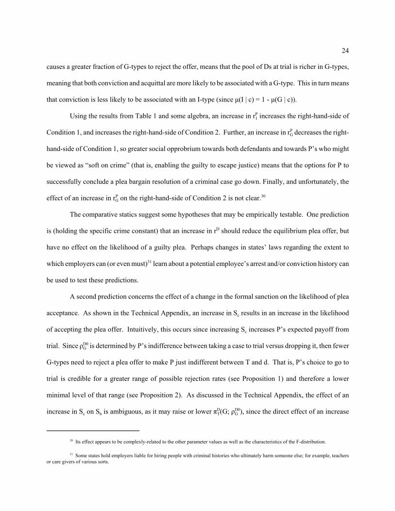
Using the results from Table 1 and some algebra, an increase in rPI increases the right-hand-side of

Condition 1, and increases the right-hand-side of Condition 2. Further, an increase in rPG decreases the right-

hand-side of Condition 1, so greater social opprobrium towards both defendants and towards P’s who might

be viewed as “soft on crime” (that is, enabling the guilty to escape justice) means that the options for P to

successfully conclude a plea bargain resolution of a criminal case go down. Finally, and unfortunately, the

effect of an increase in rPG on the right-hand-side of Condition 2 is not clear.30

The comparative statics suggest some hypotheses that may be empirically testable. One prediction

is (holding the specific crime constant) that an increase in rD should reduce the equilibrium plea offer, but

have no effect on the likelihood of a guilty plea. Perhaps changes in states’ laws regarding the extent to

which employers can (or even must)31 learn about a potential employee’s arrest and/or conviction history can

be used to test these predictions.

A second prediction concerns the effect of a change in the formal sanction on the likelihood of plea

acceptance. As shown in the Technical Appendix, an increase in Sc results in an increase in the likelihood

of accepting the plea offer. Intuitively, this occurs since increasing Sc increases P’s expected payoff from

trial. Since ρGD0 is determined by P’s indifference between taking a case to trial versus dropping it, then fewer

G-types need to reject a plea offer to make P just indifferent between T and d. That is, P’s choice to go to

trial is credible for a greater range of possible rejection rates (see Proposition 1) and therefore a lower

minimal level of that range (see Proposition 2). As discussed in the Technical Appendix, the effect of an

increase in Sc on Sb is ambiguous, as it may raise or lower πTD(G; ρG

D0), since the direct effect of an increase

30 Its effect appears to be complexly-related to the other parameter values as well as the characteristics of the F-distribution.

31 Some states hold employers liable for hiring people with criminal histories who ultimately harm someone else; for example, teachersor care givers of various sorts.

25

in Sc makes trial worse for a G-type, but there is an indirect effect of Sc on Sb via ρGD0.

What if the cost of trial to P, kP, falls? Direct computation from equation (14) above shows that ρGD0

falls (there is no change in Sb), so again what would seem like a reason for P to pursue more trials turns out,

in equilibrium, to induce fewer trials (all I-types go to trial, as before, but fewer G-types go).

Finally, overall, anything that lowers ρGD0 (holding λ and the evidence distributions constant) will raise

P’s “conviction rate” since any Ds accepting a plea are (formally) convicted of the offense. The conviction

rate is:

λ(1 - FI) + (1 - λ)ρGD0(1 - FG) + (1 - λ)(1 - ρG

D0),

where the first two terms come from I-types and G-types who go to trial and the last term reflects G-types

who plead guilty. This reduces to 1 - λFI - (1 - λ)ρGD0FG, which is clearly increasing as ρG

D0 falls. Thus,

increases in Sc, or decreases in kP, result in increases in conviction rates.

Police Arrest and Trial Process Effectiveness

Earlier we reflected on police arrest effectiveness as involving λ being small: the intake process into

the legal system is effective if the likelihood that the police arrested an I-type is (relatively) small. From

equation (14) above reductions in λ lead to reductions in ρGD0, meaning that improvements in police arrest

effectiveness increases the likelihood of plea bargaining success, which reduces the expenditure of court

costs, since fewer cases go to trial. Moreover, given the manner in which ρGD0 enters the beliefs (see equation

(11)), in equilibrium λ’s influence cancels out, so the beliefs μ(G | a) and μ(I | c) are independent of λ. Thus,

the intervening bargaining game between arrest and trial eliminates the impact of the prior λ on the

equilibrium posterior assessments about the results of trial that Θ makes.

We are also interested in the effectiveness of the trial process at properly convicting the guilty and

acquitting the innocent. If trials were perfect discriminators of guilt or innocence, we would have FI = 1 (all

innocent Ds are acquitted) and FG = 0 (all guilty Ds are convicted). While this thought experiment does not

seem possible to achieve, it does inform us about what we want investment in trial resources to do (such

investments might involve better procedures for obtaining and vetting evidence, or improved procedures for

26

the trial itself).

Let z be a level of investment in trial resources, and now extend our earlier notation F(γc | t) to

incorporate investment z:

F(γc | t, z), t = I, G,

denotes the probability that type t’s evidence draw yields an acquittal if the investment level is z and the

evidentiary standard for conviction is γc. Following our earlier example of a perfect trial, this means that we

want to require that:

FIz / MF(γc | I, z)/Mz > 0 and FGz / MF(γc | G, z)/Mz < 0.

Such an investment would increase trial effectiveness (we abstract from concerns about the cost of such

investments). Some investments may only affect FI or FG, while some might affect both.

Again, returning to equation (14), an increase in z that only affects FG thereby increases the only the

denominator of ρGD0, meaning that such an investment increases the likelihood of plea-bargaining success. The

stand-alone effect of z via FI is more complicated. This is because of the relationship between Sc and rPI.

Recall that MR1 required that (Sc - rPI)(1 - FI) - k

P < 0: if P (and Θ) know that D was of type I, P should prefer

to drop the case rather than take the case to trial. However, this does not determine the sign of Sc - rPI. If this

term is positive, then from P’s perspective, her payoff (abstracting from the cost of trial) from a conviction

of an innocent D exceeds the informal sanction rate, while if this term is negative, it means that the informal

sanction rate outweighs the utility P gains from obtaining the formal sanction.

Now we can turn to the question of an investment that improves the likelihood of acquitting an

innocent D. If the informal sanction rate is small (“small rPI,” meaning Sc - r

PI > 0), then an increase in z leads

to an increase in FI, which leads to an increase in ρGD0, which means less settlement, and higher plea offers as

well (since Sb(ρGD0) also rises in equilibrium). If the informal sanction rate is large (“large rP

I,” meaning Sc -

rPI < 0), then an increase in z leads to an increase in FI, which leads to a decrease in ρG

D0, which means more

settlement, and lower plea offers as well (since Sb(ρGD0) also falls in equilibrium). Putting this together with

the effects on FG, we see that the effect of an increase in z in the large-rPI case definitely leads to a reduction

27

in ρGD0 (and in Sb(ρG

D0)), as the numerator of equation (14) is falling while the denominator of equation (14) is

increasing. Here, trial is becoming clearly more effective at separating I-types and G-types and providing

them with the corresponding dispositions of a and c, respectively: trial is a better tool for not convicting the

innocent and for convicting the guilty. Sadly, this clarity is not present in the small-rPI case when investment

affects both FI and FG because it is not possible to sign the effect of z on ρGD0, since both the numerator and

the denominator of equation (14) are increasing.

4. Refining the Jury’s Assessment: The Scottish Verdict

For almost 300 years, Scotland has used a three-outcome verdict for criminal juries; a defendant is

found not guilty, or not proven, or guilty, with no formal sanction attaching to the first two outcomes.32 Such

a refinement of the jury’s assessment of a defendant’s guilt or innocence should provide more information

to the outside observers to employ in applying informal sanctions. Does it and, if so, what else does it do?

To address this extension, we strengthen an earlier assumption about the distribution F(e | t). We

assume that F is differentiable in e and that the strict monotone likelihood ratio property (SMLRP) holds:

SMLRP: f(e | G)/f(e | I) is strictly increasing in e, for e in (0, 1). (15)

As discussed in the Technical Appendix, this assumption implies (see Figure 1 for the weak versions in

Müller and Stoyan, 2002): 1) F(e | I) > F(e | G) (strict stochastic dominance by G); 2) f(e | G)/(1 - F(e | G))

> f(e | I)/(1 - F(e | I)) (strict hazard rate dominance by G); and 3) f(e | G)/F(e | G) > f(e | I)/F(e | I) (strict

reverse hazard rate dominance by G). We represent the three-outcome verdict by the triple {ng, np, g}, with

the obvious interpretation, and assume that γg / γc (that is, the same evidentiary standard for a conviction

under the previous two-outcome verdict is used to find a defendant “guilty” under the three-outcome

32 See Duff (1999) for an extensive discussion of the history of the development of this institution; he indicates that not proven verdictsare reached by juries in approximately one-third of the acquittals. Bray (2005) indicates that the same three-outcome verdict was used in the 1807trial of Aaron Burr for treason. Also, see Leipold (2000) for a discussion of the “California Alternative” wherein an acquitted defendant can petitionthe court for a declaration of factual innocence. While this two-stage process seems similar to the three-verdict approach in Scotland, Leipold (2000,p. 1324) indicates that California imposes “a nearly prohibitive burden of proof” on the defendant, as the defendant must prove that there was “noreasonable cause to believe that he committed the crime.” As Leipold observes, this results in relatively few defendants pursuing this remedy.

28

verdict).33 Further, let γng be the cutoff for not guilty versus not proven, where 0 < γng < γg . Thus, we extend

the previous notation so that Ft(γg) / Pr{e < γg | t} and Ft(γng) / Pr{e < γng | t}, for t = I, G.

In the Technical Appendix we show that:

1) For any non-zero vector of strategies by D, (ρGD, ρ I

D), Θ’s beliefs as to D’s likelihood of being of

type G, having observed one of the mutually-exclusive outcomes ng, np, or g, satisfies:

μ(G | ng) < μ(G | ng) < μ(G | g); (16)

and 2) that I’s expected loss from proceeding to trial (πTD(I)) is strictly lower than G’s expected loss from

proceeding to trial (πTD(G)), where:

πTD(t) = Sc(1 - Ft(γg)) + kD + rDμ(G | g)(1 - Ft(γg)) + rDμ(G | ng)Ft(γng)

+ rDμ(G | np)(Ft(γg) - Ft(γng))}, t 0 {I, G}. (17)

As earlier, the ordering of payoffs indicated above means that Proposition 1 applies to the modified game,

so that the family of equilibria again involve I-types always rejecting the plea offer and P always taking any

D who rejects a plea offer to trial, while G-types mix between accepting the plea offer and rejecting it with

probability ρGD. Similarly, P’s expected payoff from trial (πT

P) can be extended to allow for the three outcomes

but, as shown in the Technical Appendix, this function is independent of γng. This means that since ρGD makes

P indifferent between dropping and going to trial, then the equilibrium values for ρGD are the same as in the

two-outcome verdict regime. Thus, ρGD 0 [ρG

D0, 1], as before. This occurs because P’s reduced-form expected

payoffs from trial simply reflect whether D is found guilty or is acquitted. Furthermore, as shown in the

Technical Appendix, Conditions 1 and 2 now hold for a larger range of the parameter rD, so the use of the

three-outcome verdict means that informal sanctions are less likely to interfere with plea bargaining.

Proposition 2 carries over to the modified game as well: the selected equilibrium value for ρGD is the same as

earlier, ρGD0.

33 One might wonder whether the introduction of the partitioning of acquittal into not guilty and not proven might cause juries to effectivelyadjust the evidentiary standard used to convict. Not surprisingly, there is not much evidence about this (we have assumed no change). Our assumptionis consistent with results in the only experimental work of which we are aware; three psychologists consider just this issue in a series of laboratoryexperiments (see Smithson, et. al., 2007) and find that the introduction of the third verdict option does not significantly alter the likelihood of aconviction (p. 492). They also find that reported assessments of guilt follow the same montonicity as shown in our equation (16) below.

29

The change in the number of possible verdict outcomes affects Θ and D. The difference between the

regret functions for the two-outcome verdict and the three outcome verdict is that now the term

μ(G | np)(Ft(γg) - Ft(γng)) + μ(G | ng)Ft(γng) replaces μ(G | a)Ft(γg) in the computation. This change also

appears in D’s expected cost from the three-outcome trial verdict. Using the assumption SMLRP, we show

in the Technical Appendix that the following result holds:

μ(G | np)(FG(γg) - FG(γng)) + μ(G | ng)FG(γng) > μ(G | a)FG(γg), (18a)

and μ(G | np)(FI(γg) - FI(γng)) + μ(G | ng)FI(γng) < μ(G | a)FI(γg). (18b)

The implication of inequalities (18a) and (18b) is summarized in Proposition 3.

Proposition 3: The expected cost for a D of type G is higher under the three-outcome verdict than

under the two-outcome verdict. The expected cost for a D of type I is lower under the three-outcome

verdict than under the two-outcome verdict.

This means that while a G-type still rejects the equilibrium plea offer at the same rate as before, ρGD0, the

equilibrium offer itself is larger, since Sb(ρGD0) = πT

D(G; ρGD0) - rD, but the expected cost for the G-type has gotten

worse (a larger loss). Thus, P’s overall payoff increases (since the plea bargains are tougher and are accepted

at the same rate, and P’s trial payoff is unchanged). Finally, it is also straightforward to show that Θ’s

expected regret is lower in the three-outcome verdict regime. We take this to mean that, overall, use of the

Scottish verdict would enhance justice: the I-types lose less, G-types lose more, and Θs impose fewer

erroneous informal sanctions.

Further Assessment Refinement

Clearly the foregoing analysis suggests that schemes that might provide more precision with respect

to the jury’s assessment may be socially valuable. One should be cautious, however, in how this is

implemented. For example, transcripts of trials are generally pubic records, but few people wish to expend

the effort cost of obtaining and reading them, and the transcripts lack information about the visual or vocal

30

cues that the jury observed during testimony (which the jury used to assess credibility).34 Televised trials

(which occur only for a rare, selected, subset of trials) often involve extra-legal commentary, introducing

expert (and/or incompetent) opinion and evidence that was not contemplated by the jury. Thus, a prescription

to “reveal e” might, in reality, not be as useful as it seems. Since the jury is aggregating the information into

a judgment, a suitable question is what other judgments about the defendant would be informative?

One purely theoretical possibility is that the jury might choose to award compensation to D upon

acquittal, with the level of compensation adjustable to reflect the assessed degree of innocence. Thus, a D

that the jury finds to be very likely to be innocent might get a large monetary compensation. Juries compute

compensation in civil cases all the time (including complex allocations of losses between a plaintiff and a

defendant). Moreover, if the size of such an award affects the prosecutor’s career prospects (for example,

via internal reviews or public disclosure before elections), this may further incentivize her to screen

defendants more carefully.

5. Summary and Further Discussion

Our model considers the strategic interaction between a prosecutor and a defendant when informal

sanctions by third parties can be imposed on both the defendant and the prosecutor. These sanctions affect

the feasibility of plea bargaining, as well as the level of the bargain offered and the frequency of bargaining

success. The model follows the action from choosing a plea offer up through trial, allowing for dropping of

cases, thereby not relying on prosecutors being able to pre-commit to taking defendants who reject offers to

trial. The defendant’s private information concerns his guilt or innocence of the crime for which he was

arrested; this underlying state of the world affects the evidence that is presented at trial. Third parties form

beliefs about the defendants who are processed through the system, allowing for outcomes wherein a plea is

34 This is why appeals courts in the U.S. do not use the trial record to re-try the case (or incorporate new evidence) and gives deferenceto the jury’s decision; if there appears to have been a procedural error (for example, evidence was included that should have been excluded), theappeals court will order a new trial with a new jury again seeing evidence presented in court.

31

accepted, or a case is dropped, or a defendant goes to trial and is convicted or acquitted. Significantly, while

the third parties can observe the disposition of the cases, they cannot observe plea offers or evidence

generation; of course they are rational and can construct the equilibrium of the game, but the errors in the

legal process (as well as hidden information) means that they will misclassify defendants and thereby

erroneously impose sanctions on both defendants and prosecutors.

We show that there is a unique family of equilibria and, if third parties prefer a legal system with

minimal regret arising from classification errors, a unique equilibrium within this family, wherein the guilty

defendant accepts the prosecutor’s proposed plea offer with positive (but fractional) probability, the innocent

defendant rejects the proposed offer, and the prosecutor chooses to take all defendants who reject the offer

to trial. The plea offer and the decisions by each agent are all a function of the informal sanctions.

We find that informal sanctions may act to constrain the set of possible plea offers the prosecutor can

make, but informal sanctions on the prosecutor can work in opposite directions depending upon whether the

concern is for convicting the innocent or letting the guilty escape justice. If the informal sanction rate on

defendants is high enough (if society is sufficiently condemning of those agents who are arrested), then plea

bargaining is eviscerated. High potential sanctions on prosecutors can also lead to distortions, with high

sanctioning of prosecutors for likely conviction of innocents leading to tougher plea offers, and more guilty

defendants rejecting the plea offer and going to trial, which increases the association between any trial

outcome (conviction or acquittal) and guilt. Alternatively, high potential informal sanctions of prosecutors

for perceived release of the guilty (“soft on crime”) leads to greater use of plea bargaining, as offers are made

less tough (acceptance of an offer by a defendant self-labels them as guilty, so prosecutors do not suffer any

informal sanctions following a plea bargain offer that is accepted).

We further consider the importance of police effectiveness (that police have a solid basis for an arrest

in the first place, thereby reducing the likelihood that innocents are swept up into the process) as well as trial

effectiveness (the degree to which evidence acts to correctly classify defendants as to their guilt). Increased

police effectiveness leads to greater use of plea bargaining to resolve offenses, and thereby saves trial costs.

32

Increased investment in the trial process, when informal sanctions on prosecutors for possibly “railroading”

innocents (that is, rPI) is sufficiently high, has a clear result of enhancing the effectiveness of plea bargaining;

results are less clear if the informal sanctions are less important to the prosecutor than her utility for the

formal sanction associated with conviction at trial.

Finally, we examined the effect of extending the analysis to the “Scottish” (three-outcome) verdict,

wherein juries find a defendant not guilty, not proven, or guilty. We showed that the propositions proved

earlier carry over to the new regime. In particular, the same equilibrium obtains, including the same

likelihood of bargaining success, with the only modification being that the equilibrium settlement offer is

higher. This reflects the result that, at trial, guilty defendants do worse under this scheme while innocent

defendants do better. Moreover, outside observers impose informal sanctions with a lower total regret

associated with erroneous application. Overall, the Scottish verdict leads to an increase in justice.

Further Discussion Concerning Maintained Assumptions and Possible Extensions

An important assumption made in the model is that all agent payoffs are linear in sanctions, both

formal and informal (see the payoffs in Section 2). This provided an important result: innocent defendants

expect a smaller loss from proceeding to trial than guilty ones (Remark 1). Using this result contributes to

the further result that we can (at least partly) separate the guilty from the innocent via a plea offer, with (in

equilibrium) all innocent defendants rejecting the offer, and some guilty defendants also rejecting it.

It is quite possible that defendants may have a nonlinear response to risk, and the implications for

our equilibria may be significant.35 If the G-types are less risk-averse (or possibly even risk-taking) in

comparison with I-types, then Remark 1 may not hold. This, in turn, would alter the type of equilibrium for

the game. For example, the payoffs might reverse their ordering and we might have guilty defendants

electing trial and innocent defendants being willing to accept a plea offer. Or, more interestingly, neither

payoff would dominate for all possible distributions of evidence, leading to an equilibrium wherein a fraction

35 Becker (1968) suggests that offenders (G-types) may be risk-takers, while law-abiding citizens may be risk-avoiders.

33

of both types accept a plea offer. We view this as a worthwhile, but very complex, extension.36

A second direction of extension would be to provide a more complete model of the trial, especially

the generation of evidence. In the current analysis, the only conditioning variable for the F-distribution is

the underlying guilt or innocence of the defendant. If the prosecutor could make an investment in evidence

production, possibly based on what she inferred from the plea bargaining outcome, that might affect both the

trial and the plea bargaining process itself (especially if plea bargaining was modeled as – say – an

alternating-offer process, rather than a take-it-or-leave-it offer as we do above). Of course, allowing the

prosecutor to make such investments suggests allowing the defendants to do this as well, and that suggests

a more sophisticated model of the jury’s decision process might also be warranted.37

Third, one might use the model to consider possible social policies to rectify the inaccuracies inherent

in the use of informal sanctions; we briefly speculated about this in Section 4. Should society compensate

those who are acquitted for their trial costs? For the inevitable informal sanction that they face, even though

they are acquitted? How would the presence of such a subsidy impact plea bargaining? Would greater

transparency of the legal process further help reduce misapplication of informal sanctions? We have the jury

following a simple rule (i.e., not drawing an inference from the level of the evidence, e, as to the underlying

distribution – and therefore type of D). What if (as suggested in Section 4) outside observers could acquire

a more detailed version of the jury’s assessment of the defendant’s guilt or innocence and draw inferences

based on it? Both of these suggestions (subsidies and transparency) would involve substantial modifications

to the game, but could lead to interesting implications and policy proposals.

Finally, another possible direction of extension concerns how informal sanctions affect deterrence

36 If G-types are more likely to have experience with the legal process than I-types, then it is possible that G-types can better anticipatethe relevant details of the distribution associated with evidence, F, while I-types might be unsure about the F-distribution that would apply. That is,perhaps I-types are ambiguity averse, and this, too, would affect payoffs. For a recent application of ambiguity aversion to civil suits, see Franzoni(2014).

37 It may also be worth noting that police effectiveness might affect the distributions of evidence as well, which might cause the observers’equilibrium posterior beliefs to be influenced by the prior.

34

and the application of both formal and informal sanctions.38 This extension necessitates expanding the model

so as to allow for a socially-optimal choice of the statutory sanction for convictions, Sc. The presence of

informal sanctions should affect the socially optimal level of the formal sanctions, though the direction is

unclear. Informal sanctions on the defendant suggest that the statutory sanction would be lower (assuming

that the existing level ignored the possibility of informal sanctions), since it is the total level that would

influence the person committing the crime, and incarceration implies costs due to maintaining facilities as

well as any productivity losses. Thus, this might lead to lower plea offers, but lower statutory sanctions

coupled with informal sanctions on prosecutors could lead to reduced incentives for prosecutors, which may

be undesirable. Whether improved deterrence would have any effect on the observers’ expected regret in the

application of the informal sanctions would also be worth evaluating.

38 See Reinganum (1993) for an example of a model with criminals choosing whether to commit a crime, police potentially detecting acrime committed, and plea bargaining with a prosecutor if arrested.

35

References

Associated Press, “Day in Jail for Ex-Duke Prosecutor,” New York Times, September 1, 2007. Online athttp://www.nytimes.com/2007/09/01/us/01nifong.html; accessed on May 20, 2014.

Baker, Scott, and Mezzetti, Claudio, “Prosecutorial Resources, Plea Bargaining, and the Decision to Go toTrial,” Journal of Law, Economics, and Organization, 17(1), 2001, pp. 149-167.

Bandoyopadhyay, Siddhartha, and McCannon, Bryan C., “The Effect of the Election of Prosecutors onCriminal Trials,” Public Choice, forthcoming 2014.

Becker, Gary S., “Crime and Punishment: An Economic Approach,” Journal of Political Economy, 76(2),1968, pp. 169-217.

Benabou, Roland, and Tirole, Jean, “Incentives and Prosocial Behavior,” American Economic Review 96(2006), 1652-1678.

Bjerk, David, “Guilt Shall not Escape of Innocence Suffer: The Limits of Plea Bargaining When DefendantGuilt is Uncertain,” American Law and Economics Review, 9(2), 2007, pp. 305-329.

Boylan, Richard T., and Long, Cheryl X., “Salaries, Plea Rates, and the Career Objectives of FederalProsecutors,” Journal of Law and Economics, 48(2), 2005, pp. 627-652.

Boylan, Richard T., “What do Prosecutors Maximize? Evidence from the Careers of U.S. Attorneys,”American Law and Economics Review, 7(2), 2005, pp. 379-402.

Bray, Samuel, “Not Proven: Introducing a Third Verdict,” The University of Chicago Law Review, 72(4),2005, pp.1299-1329.

Burke, Mary Kate; Hopper, Jessica; Francis, Enjoli; and Effron, Lauren, “Casey Anthony Juror: ‘Sick to OurStomachs’ Over Not Guilty Verdict,” ABC News, July 6, 2011. Online at:http://abcnews.go.com/US/casey_anthony_trial/casey-anthony-juror-jury-sick-stomach-guilty-verdict/story?id=14005609

Daughety, Andrew F., and Reinganum, Jennifer F., “Public Goods, Social Pressure, and the Choice BetweenPrivacy and Publicity,” American Economic Journal: Microeconomics 2 (2010), 191-221.

Deffains, Bruno, and Fluet, Claude, “Legal Liability when Individuals Have Moral Concerns,” Journal ofLaw, Economics, and Organization 29 (2013), 930-955.

Duff, Peter, “The Scottish Criminal Jury: A Very Peculiar Institution,” Law and Contemporary Problems,62(2), 1999, pp. 173-201.

Franzoni, Luigi A., “Negotiated Enforcement and Credible Deterrence,” The Economic Journal, 109, 1999,pp. 509-535.

Franzoni, Luigi A., “Liability Law and Uncertainty Spreading,” Working Paper, Department of Economics,University of Bologna, February, 2014.

36

Glaeser, Edward L., Kessler, Daniel P., and Piehl, Anne Morrison, “What do Prosecutors Maximize? AnAnalysis of the federalization of Drug Crimes,” American Law and Economics Review, 2(2), 2000, pp. 259-290.

Gordon, Sanford C., and Huber, Gregory A., “Citizen Oversight and the Electoral Incentives of CriminalProsecutors, American Journal of Political Science, 46(2), 2002, pp. 334-351.

Grossman, Gene M., and Katz, Michael L., “Plea Bargaining and Social Welfare, The American EconomicReview, 73(4), 1983, pp. 749-757.

Landes, William M., “An Economic Analysis of the Courts,” Journal of Law and Economics, 14(1), 1971,pp. 61-108.

Leipold, Andrew D., “The Problem of the Innocent, Acquitted Defendant,” Northwestern University LawReview, 94(4), 2000, 1297-1356.

McCannon, Bryan C., “Prosecutor Elections, Mistakes, and Appeals,” Journal of Empirical Legal Studies,10(4), 2013, pp. 696-714.

Müller, Alfred, and Stoyan, Dietrich, Comparison Methods for Stochastic Models and Risks, John Wiley andSons, England, 2002.

Nalebuff, Barry, “Credible Pretrial Negotiation, The RAND Journal of Economics, 18(2), pp. 198-210.

NC State Bar v. Michael B. Nifong, Disciplinary Hearing Commission, NC State Bar, 06 DHC 35. Onlineat http://www.ncbar.com/discipline/printorder.asp?id=505

Reinganum, Jennifer F., “Plea Bargaining and Prosecutorial Discretion,” The American Economic Review,78(4), 1988, pp. 713-728.

Reinganum, Jennifer F., “The Law Enforcement Process and Criminal Choice,” International Review of Lawand Economics, 13(2), 1993, pp. 115-134.

Smithson, Michael; Deady, Sara; and Gracik, Lavinia, “Guilty, Not Guilty, or ...? Multiple Options in JuryVerdict Choices,” Journal of Behavioral Decision Making, 20(5), 2007, pp. 481-498.

Segal, David, “Mugged by a Mug Shot Online,” New York Times, October 5, 2013. Online athttp://www.nytimes.com/2013/10/06/business/mugged-by-a-mug-shot-online.html?pagew; accessed on May20, 2014.

37

Appendix

Characterizing EquilibriaThe only candidates for an equilibrium involve ρ I

D = 1 (I-types always reject the plea offer) and ρGD

0 (0, 1] (G-types reject the plea offer with positive probability); see the Technical Appendix wherein othercandidates are ruled out. P may also mix between taking the case to trial and dropping it following rejection.

The timing of the game is such that each type of D chooses to accept or reject the plea offer, takingas given the likelihood that P takes the case to trial following rejection; and P chooses to take the case to trialor drop it, given her beliefs about the posterior probability that D is of type G, given rejection. Both of thesedecisions are taken following P’s choice of plea offer, SP, so both parties must take this offer as given atsubsequent decision nodes.

We first characterize the equilibrium in the continuation game, given Sb, allowing for mixed strategiesfor both P (ρP) and the D of type G (ρG

D). Since the observers’ beliefs will depend on their conjectured valuefor ρG

D, we will augment the notation for the observers’ beliefs to reflect these conjectures, ρGDΘ. Other

functions that also depend on these conjectures through the observers’ beliefs will be similarly augmented.

Suppose that observers conjecture that the D of type G rejects the plea offer with probability ρGDΘ.

Then μ(G | c; ρGDΘ) = ρG

DΘ(1 - λ)(1 - FG)/[ρGDΘ(1 - λ)(1 - FG) + λ(1 - FI)]; μ(G | a; ρG

DΘ) = ρGDΘ(1 - λ)FG/[ρG

DΘ(1 - λ)FG

+ λFI]; μ(G | d; ρGDΘ) = ρG

DΘ(1 - λ)/[ρGDΘ(1 - λ) + λ]; and μ(G | b; ρG

DΘ) = 1. Moreover, suppose that the D of typeG anticipates these beliefs, and also expects that P will take the case to trial following rejection withprobability ρP. Then type G will be indifferent, and hence willing to mix, between accepting and rejecting theoffer Sb, if πR

D(G; ρGDΘ) = ρPπT

D(G; ρGDΘ) + (1 - ρP)πd

D(ρGDΘ) = πb

D(ρGDΘ). Substitution and simplification yields the

value of ρP that renders G indifferent:

ρP(Sb; ρGDΘ) = {Sb + rD(1 - μ(G | d; ρG

DΘ))}{Sc(1 - FG) + kD + rD[μ(G | c; ρG

DΘ)(1 - FG) + μ(G | a; ρGDΘ)FG - μ(G | d; ρG

DΘ)]}.

The numerator of the expression ρP(Sb; ρGDΘ), which is the difference between type G’s payoff from

accepting the plea offer versus having his case dropped, is clearly positive, meaning that D would prefer tohave his case dropped than to accept a plea offer. The denominator of the expression ρP(Sb; ρG

DΘ) is thedifference between type G’s payoff from trial versus having his case dropped. This denominator is alsopositive (see Remark 3 in the Technical Appendix), which implies that type G would prefer that P drop thecase against him rather than take it to trial.

Since the observers’ beliefs are based on their conjectures ρGDΘ and the case disposition, and NOT on

Sb, which they do not observe, the expression ρP(Sb; ρGDΘ) is an increasing function of Sb. That is, when Sb is

higher, P must take the case to trial following rejection with a higher probability in order to make the D oftype G indifferent about accepting or rejecting Sb. Notice that even a plea offer of Sb = 0 requires a positiveprobability of trial following a rejection in order to induce the D of type G to be willing to accept it; this isbecause acceptance of a plea offer comes with a sure informal sanction of rD (as only a truly guilty D isexpected to accept the plea).

Now consider P’s decision about trying versus dropping the case. Again suppose that observers –and P – both conjecture that type G rejects the plea offer with probability ρG

DΘ in this candidate forequilibrium; thus ν(G | R; ρG

DΘ) = ρGDΘ(1 - λ)/[ρG

DΘ(1 - λ) + λ]. Since these conjectures must be the same (andcorrect) in equilibrium, it is valid to equate them at this point in order to identify what common beliefs forP and Θ will make P indifferent, and hence willing to mix, between trying and dropping the case following

38

a rejection. P will be indifferent between these two options if πTP(ρG

DΘ) = πdP(ρG

DΘ); that is, if:

ν(G | R; ρGDΘ){Sc(1 - FG) - kP - rP

Iμ(I | c; ρGDΘ)(1 - FG) - rP

Gμ(G | a; ρGDΘ)FG}

+ ν(I | R; ρGDΘ){Sc(1 - FI) - k

P - rPIμ(I | c; ρG

DΘ)(1 - FI) - rPGμ(G | a; ρG

DΘ)FI} = - rPGμ(G | d; ρG

DΘ).

Substituting for the beliefs and solving for the value of ρGDΘ that generates this equality (see the Technical

Appendix for details) yields:

ρGD0 = - λ[(Sc - r

PI)(1 - FI) - k

P]/(1 - λ)[(Sc + rP

G)(1 - FG) - kP],

where the numerator is positive by MR1; MR2 implies that the denominator is positive and the ratio is afraction. For any ρG

DΘ > ρGD0, P will strictly prefer to take the case to trial following a rejection, and for any

ρGDΘ < ρG

D0, P will strictly prefer to drop the case following a rejection.

To summarize, type G is willing to mix between accepting and rejecting the plea offer Sb if heanticipates that the observers’ beliefs are ρG

DΘ = ρGD0 and he expects that P will take the case to trial following

rejection of offer Sb with probability ρP(Sb; ρGD0). P is indifferent between trying and dropping the case if she

and the observers believe that type G rejects the plea offer with probability ρGD0. Thus, the mixed-strategy

continuation equilibrium, given Sb, is (ρGD0, ρP(Sb; ρG

D0)).

We can now move back to the decision node at which P chooses the plea offer Sb, anticipating thatit will be following by the mixed-strategy equilibrium (ρG

D0, ρP(Sb; ρGD0)) in the continuation game. P’s payoff

from making the plea offer Sb is:

(1 - ρGD0)(1 - λ)Sb + (ρG

D0(1 - λ) + λ)[ρP(Sb; ρGD0)πT

P(ρGD0) + (1 - ρP(Sb; ρG

D0))πdP(ρG

D0)].

The set of Sb values that support some plea acceptance is bounded below by 0 and above by Sb =πT

D(G; ρGD0) - rD, where πT

D(G; ρGD0) is the expression for πT

D(G), evaluated at the beliefs μ(G | c; ρGD0) = ρG

D0(1 -λ)(1 - FG) /[ρG

D0(1 - λ)(1 - FG) + λ(1 - FI)]; and μ(G | a; ρGD0) = ρG

D0(1 - λ)FG/[ρGD0(1 - λ)FG + λFI]. This is because

accepting the plea offer results in a combined sanction of Sb + rD (since only guilty D’s accept the plea offer)and thus any plea offer higher than πT

D(G; ρGD0) - rD will be rejected for sure (rather than with probability ρG

D0). At this upper bound, the function ρP(Sb; ρG

D0) just reaches 1. In order for this range to be non-empty, we needπT

D(G; ρGD0) - rD > 0; or, equivalently (note that the denominator of the expression below is positive):

Condition 1. In order for P to be able to induce a D of type G to accept a plea offer, it must be that rD < [Sc(1- FG) + kD]/[1 - μ(G | c; ρG

D0)(1 - FG) - μ(G | a; ρGD0)FG].

Returning to P’s payoff as a function of Sb, notice two things. First, since ρGD0, which is independent

of Sb, renders P indifferent between trying and dropping the case following rejection, the term in squarebrackets simply equals πd

P(ρGD0) = - rP

Gμ(G | d; ρGD0), where μ(G | d; ρG

D0) = ρGD0(1 - λ)/[ρG

D0(1 - λ) + λ]. Thus, theoptimal Sb that supports some plea acceptance is Sb(ρG

D0) = πTD(G; ρG

D0) - rD. This offer is rejected by type Gwith probability ρG

D0, and P goes to trial with certainty following a rejection. Note that a D of type I wouldalways reject this plea offer, consistent with the hypothesized form of the equilibrium.

Every plea offer in the feasible set [0, πTD(G; ρG

D0) - rD] is consistent with a mixed-strategy equilibriumin which some D’s of type G accept, and others reject, the offer. But – taking the observers’ beliefs of ρG

D0

as given – P could make a higher demand that would provoke certain rejection by both D-types. We needto verify that P prefers the hypothesized equilibrium described above to the “defection payoff” she would

39

obtain if all cases went to trial.

In the hypothesized equilibrium, P settles with (1 - ρGD0)(1 - λ) guilty defendants and goes to trial

against the rest of the guilty defendants and all of the innocent defendants; if P defects and provokes rejectionby all, then she will simply replace the settlement Sb(ρG

D0) = πT

D(G; ρGD0) - rD with the expected payoff from

taking a guilty defendant to trial (holding the observers’ beliefs fixed at ρGD0). Thus, P prefers (at least weakly)

the hypothesized equilibrium to defection as long as:

πTD(G; ρG

D0) - rD = Sc(1 - FG) + kD + rDμ(G | c; ρGD0)(1 - FG) + rDμ(G | a; ρG

D0)FG - rD

> Sc(1 - FG) - kP - rPIμ(I | c; ρG

D0)(1 - FG) - rPGμ(G | a; ρG

D0)FG.

Rearranging, we can write this as:

Condition 2. For P to find it preferable to settle with a D of type G rather than provoking a trial (holding theobservers’ beliefs fixed at ρG

D0), it must be that:

rD < [kP + kD + rPIμ(I | c; ρG

D0)(1 - FG) + rPGμ(G | a; ρG

D0)FG]/[1 - μ(G | c; ρGD0)(1 - FG) - μ(G | a; ρG

D0)FG].

Finally, P could also defect by dropping all cases; again, this would not change the observers’ beliefs,but we need to verify that P prefers the hypothesized equilibrium outcome to what she would get by defectingto dropping all cases. However, Condition 1 is sufficient to imply this preference. To see why, notice thatin the hypothesized equilibrium, P’s payoff is:

(1 - ρGD0)(1 - λ)[πT

D(G; ρGD0) - rD] + (ρG

D0(1 - λ) + λ)πTP(ρG

D0).

We already know that πTP(ρG

D0) = πdP(ρG

D0) by construction. Then Condition 1 implies that the settlement offerSc(ρG

D0) = πTD(G; ρG

D0) - rD is non-negative, whereas P’s payoff from dropping a case is - rPGμ(G | d; ρG

D0), whichis strictly negative. Thus, P strictly prefers the outcome involving some plea bargaining to defecting todropping all cases.

Multiple EquilibriaThere can also be equilibria wherein the D of type G rejects the plea bargain with probability ρG

D >ρG

D0. The reason for this multiplicity of equilibria is that the observers’ beliefs actually drive the equilibriumbehavior of P and the D of type G. To see this, suppose that ρG

DΘ = ρGD1 > ρG

D0, and that P and type G anticipatethese beliefs. Since the observers’ posterior beliefs μ(G | c; ρG

DΘ) and μ(G | a; ρGDΘ) are increasing in ρG

DΘ, bothP and the D of type G expect that D will face harsher informal sanctions following either trial outcome (thanthey would face at ρG

D0).

This means that P can demand the higher plea sentence, Sb(ρGD1) = πT

D(G; ρGD1) - rD, which will make

the D of type G indifferent about accepting and rejecting it (if he expects P to take the case to trial followinga rejection); thus, type G is willing to randomize and reject the plea bargain with probability equal to ρG

D1. Since ρG

D1 > ρGD0, P will take the case to trial with probability 1 following a rejection (if he thinks that the D

of type G is using the rejection probability ρGD1). Thus, there is an equilibrium at any ρG

D 0 [ρGD0, 1) as long as

Conditions 1 and 2 continue to hold at that ρGD.

Since P prefers to settle via plea bargain rather than going to trial against type G when Condition 2holds, and P strictly prefers to go to trial (rather than drop) following rejection when ρG

D > ρGD0, why can’t P

offer a slightly lower plea offer than Sb(ρGD) = πT

D(G; ρGD) - rD and induce type G to accept with probability 1?

40

The reason is that P needs to maintain her own incentives to go to trial following rejection. If P were to offera slightly lower plea offer designed to induce type G to accept for sure, then G should expect the case to bedropped following rejection (since P’s subsequent beliefs should be that every rejection is coming from a Dof type I). This will cause type G to reject this offer, despite its apparent allure. Consequently, P cannot gainby deviating to a lower plea offer.

Selecting Among EquilibriaThe following terms summarize erroneously-imposed informal sanctions. Excessive sanctions

imposed on type I defendants following conviction, or acquittal, at trial (ideally, there would be no sanctions):

λ(1 - FI)rDμ(G | c) + λFIr

Dμ(G | a).

Insufficient sanctions imposed on type G defendants following conviction, or acquittal, at trial(ideally, the sanction would be rD):

ρGD(1 - λ)(1 - FG)[rD - rDμ(G | c)] + ρG

D(1 - λ)FG[rD - rDμ(G | a)].

Prosecutors also suffer erroneously-imposed sanctions. With respect to innocent defendants:

λ(1 - FI)[rPI - r

PIμ(I | c)] + λFI[r

PGμ(G | a)].

Note that the first term reflects the fact that P convicted a type I and ideally would have received the sanctionrP

I, but she only received rPIμ(I | c); the second term reflects the fact that an innocent was acquitted, but P was

still sanctioned because observers’ beliefs admit some probability that the acquittal was an error, for whichP is sanctioned (undeservedly).

With respect to guilty defendants:

ρGD(1 - λ)(1 - FG)[rP

Iμ(I | c)] + ρGD(1 - λ)FG[rP

G - rPGμ(G | a)].

The first term reflects the fact that P convicted a guilty D, but was still sanctioned because observers’ beliefsadmit some probability that the conviction was an error, for which P is sanctioned (undeservedly); the secondterm reflects the fact that a guilty D was acquitted, so P ideally would have received the sanction rP

G but onlyreceived rP

Gμ(G | a).

Let R(ρGD) denote the measure of “expected regret” that observers experience due to these erroneous

sanctions. Then (all of the observers’ beliefs are evaluated at ρGD):

R(ρGD) = λ(1 - FI)r

Dμ(G | c) + λFIrDμ(G | a) + ρG

D(1 - λ)(1 - FG)[rD - rDμ(G | c)] + ρG

D(1 - λ)FG[rD - rDμ(G | a)] + λ(1 - FI)[rPI - r

PIμ(I | c)] + λFI[r

PGμ(G | a)]

+ ρGD(1 - λ)(1 - FG)[rP

Iμ(I | c)] + ρGD(1 - λ)FG[rP

G - rPGμ(G | a)].

Collecting terms simplifies the above expression greatly:

R(ρGD) = (rD + rP

I){λ(1 - FI)μ(G | c) + ρGD(1 - λ)(1 - FG)μ(I | c)}

+ (rD + rPG){λFIμ(G | a) + ρG

D(1 - λ)FGμ(I | a)}.

Upon recalling the definitions of μ(t | y), and evaluating them at ρGD), it is straightforward (though tedious)

to show that both of the terms in curly brackets in the expression R(ρGD) are increasing in ρG

D.