120.~ \ 7~8

~ "Proj ect 264,;?1#

INFLUENCE SURFACES FOR BRIDGE SLABSBY

TADAHIKO KAWAI

May 2 9 1957

A. INTRODUCTION.''>- '<,

FRITZ ENGINEERINGLABORATORY LIBRARY

The use of influence lines for the design of bridges sUb-

jected to live loads has become a standard practice, even to the

extent that no other method is accepted.

The influence lines allow the determination of the maximum

mOment, shearing force, axial load, etc. for a given section in a

bridge me~ber under live loads. A logical extension of this

method; to the design of bridge slabs is the development of in-, .'

fluence surfaces (two,-dimensional influence lines).' ,They ~a11ow'-

. .: ~

to determine the maximum moment (and shearing force, tWi,s~lng

moments etc.', if desired) at a given point of the slab subjected

to concentrated wheel loads. The proper detail,ing of the .'slab

can be readily handled, once the extreme moment values are known.

It is quite evident that use of influence surfaces to determine

the maximum bending moments in the slab will lead to more e~on-

, . .

'omical designs than the present semi-empirical rules.

B. ENGINEERING CONCEPT OF INFLUENCE SURFACES

(I) Mathematical Th~ory of Influence Lines(Theory of Green's Functions of Beams)

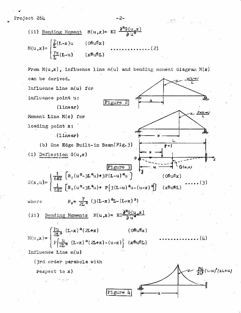
(a) Simply Supported Beam

(1) Deflection G(u,i}

(Figure 1)

IP(L-x )u (2L (L-u) - (L-x) 2_ (L_u)2 ]G( )

I 6EIL 'u x ==

, . Px(L-u) (2L(L-X)-(L-u)2_(L-x)2), 6ElL

Ie

(O~u~x) .

•••• (I)(x~u~L)

Lp=1

"

---------

..'

..Project 264 -2-

(ii) Bending Moment

, {E(L-X)UM(u,x)= L, iX(L-U)

(():€u~X )••••• 0 ••• 0.0 •• (2)

F'rom M(u,x), influence line m{u) and bending moment diagram:M(x)

loading point x:

(l;inear)

(b) One Edge Built-in Beam(Fig.3)

( i) 'Defle.s,tion G(u,x)

fX(L-tt.}

L

1.1.(L-u}L

• • • • • (3)

(~u~x)

o r----'J---I--f----_=-:-::-:-...---t--........~- x

IFigure 21

IFigure 31

[R, (tiO3-3L~)+3P(L-u)~J ~

[R I (u 3-3L 2u)+ p{ 3 (L~u) 2 U _ (u-x) iJR,= ~O3 (3(L-x)2L~(Li~)03)

can be derived.

(linear)

Moment Line M(x) for

,ltkG(x,u)= 1

6EI

Influence Line m(u) for

wheT"s

'influence point u:

(i ') a d" M t ~I( } El a2G (u,x}1, L>en :tng !·!omen s !', U,X = ' 0 U:a

T' , '. f~. 3 .. (L.I-X) 2 ( 2L+X) ( ~U~x)."'ItU,X)= p{2Lua }

(L-x) 2'(2L+X)-(U-X) (x~~L)

Ini'luencieLine m( U)

(3rd order parabola with

respect to x)

114'igure 41,

• • .'. • .. • • • • • • • • (4)

·.Project 264•

Moment Line N(x)

(linear with respect to u)

-3-

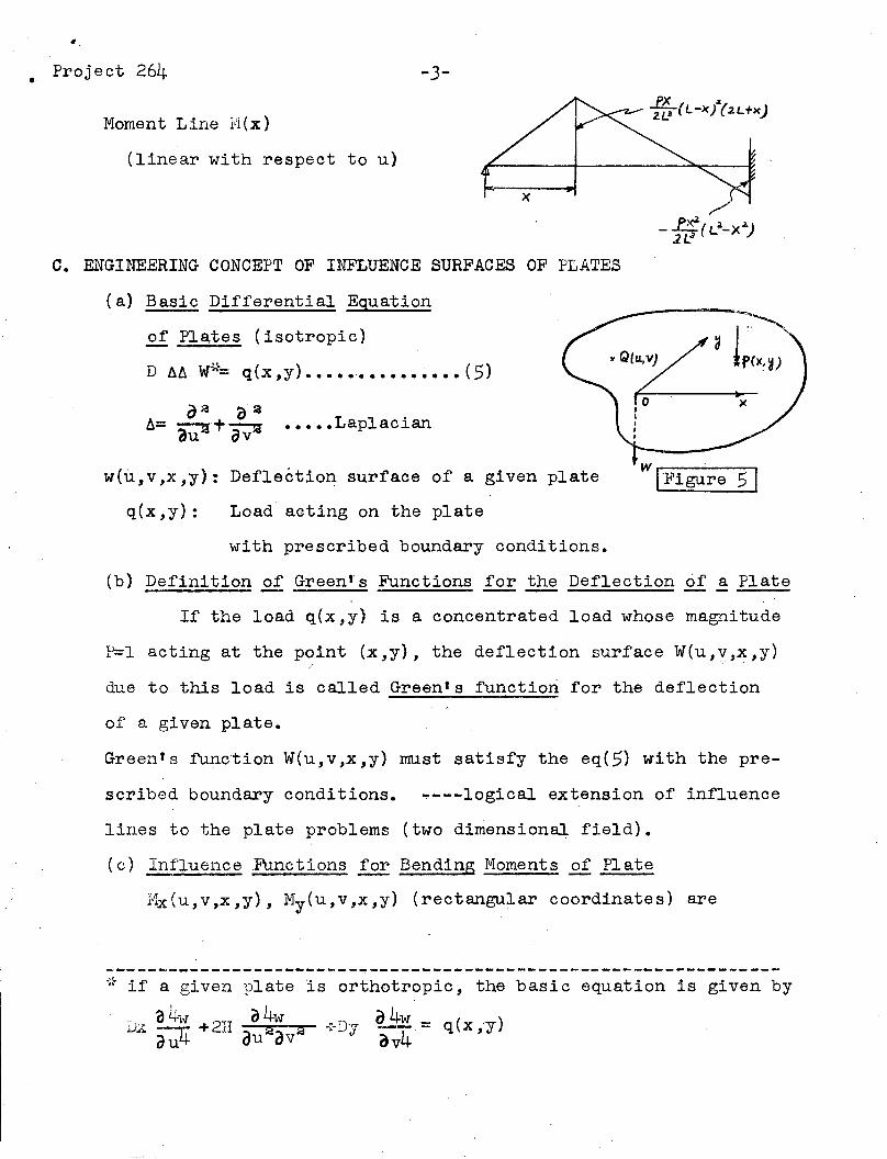
c. &~GINEERING CONCEPT OF INFLUENCE SURFACES OF PLATES

(a) Basic Differential Equation

of Pl~tes (isotropic)

D fj.fj. W~~'= q(x,y) ••••••••••••••• (5)

ala 0 2

fj.= DU2+ ov2 •••• • Laplacian

w(u,v,x,y}: Deflection surface of a given platew .

IFigure 51

q(x,y): Load acting on the plate

with prescribed boundary conditions.

(b) Definition of Green's Functions for the Deflection of a Plate

If the load q(x,y) is a concentrated load whose magnitude

P=l acting at the point (x,y), the deflection surface W(u,v,x,y)

due to this load is called Green's function for the deflection

of a given plate.

Green's function W(u,v,x,y) must satisfy the eq(5) with the pre-

scribed boundary conditions. ~---logical extension of influence

lines to the plate problems (two dimensional field).

(c) Influence Functions for Bending Moments of Plate

Mx(u,v,x,y), My(U,v,x,y) (rectangular coordinates) are

--------------------------------------~-------------------------

~w = q(x ,y)av4

';(- if a given plate is orthotropic, the

VX ~ ~li +2H ....;a:;...,~,.;,.;.~;...v.....J3,... +D-y

basic equation is given by

,

•Project 264 -4-

given by~

(d) An Example of Influence Functions.

Infinite plate strip with simply

supported parallel edges (isotropic)o I----'----.;----+__­

«. X

,Figure E?l

In1T'

Pal ~ 1 - mr ±a-( v-y) nlTUW(u,v;x,y}= 21f3D2, '!i3 (1 + "a(v-y» sirr-a

"=1

~-oomrx

sin-a

(upper sign for V ~ y)

(lower sign for V ~ y)•••••• '••• oo •• o••• o(7)

I1X(U,V;X,y)\ P ;2 1 [=_ _ (l+y)111[ ( '"'1) 21f n'l_y,U,V,x,Y 1\=1"

(

upper sign for M.x )

lower sign for My

«f?vJ•• " ••••••••••• 0 (8)

or closed form expressions:

Mx (u, V;X,y}j P [' cosh-i-( v-y) _ cos.JL( u+x); " = 'Elf (l+y) log - - :::g:My(u,v;x,y} , cos~(v-y)-cos~(u-x)

; (l-y) -f( v-y) J siuhf-( v-y) ... sinh:! ( v-y) " -lJ'1 cosh-i-(v-y)-cos-i-(u-x) cosh-!-(v-y)-cos-l-(u+x)

••••••••••••• (9)

From moment influence functions Mx(U'v;x,y), My{u,v;x,y) influence

surfaces for 111x(u,v), my(u,v) and moment surfaces for Mx(x,y) ,My(x,y)

can be derived, and those furfaces' _are~ presented by contour line dia.-~E~~~_1~~~:12 ~ ~ __~;. for y ~ v the sign' preceding (v-y) ~us t be changed.

,

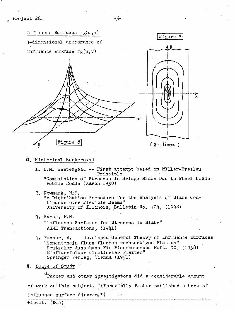
Project 264.'Influence Surfaces mx(u,v)

3-dimensional appearance of

. influence surface mx(u,v)

{Figure 81

-5-

:\:....

IFigure 71

I

( 8 1T times)

•• Historical Backgrounq

1. H.M. Westergaad -~ First attempt based on M~ller-Breslau

Principle"Computation of Stresses in Bridge Slabs Due to Wheel. Loads"Public Roads (March 1930)

2. Newmark, N,;1Vl."A Distribution Procedure for the Analysis of Slabs Con­tinuous over Flexible Beams"University of Illinois, Bulletin No. 304, (1938)

3. Baron, F.M."Influence Surfaces· for Stresses in Slabs"

ASME Transactions, (1941)

4. Pucher, A. -- developed General Theory of Influence SurfacesllHomentenein fluss fl!ichen rechteckigen Platten"Deutsch.er Ausschuss Ft!frEisenhetonbau Heft. 90, (1938)

"Einflussfelder elastischer Platten"Springev Verlag, Vienna (1951)

"E. Scope of Study ;~

.;(-Pucher and other inve!3tigators did a considerable amount

of ''lork on! this subject. . (Especially Pucher published a book of

infiuencesurface diagram~+)---------~--------~------~---------------~--~--~---------_._------+locit. (~.4) . .

,Project 264

•-6-

Unfortunately the known surfaces cover only cases of single

slabs o:f rectangular shape. The main objective of this research

program. is the development of new theoretical solutions for

a. continuous slabs

b. skewedslabs

Co orthotropic slabs

d. slabs on elastic foundationsI

e. flatslabs

f'. study of possibility to determine the influence

surfaces by experiments for unusual cases.

F. APPLICATION OF INFLUENCE SURFACES

(i) for a distributed load p(x,y)

M(u,v)= Jf p(x,y) m(u,v;x,y) dXdy

(ii) for a line load p(s)

M(u,v)= !p(s) m(u,v;x,y} ds

(iii) for several concentrated loads Pi(xi,yi)

M(u,v)= Z'Pi(Xi,Yi) m(u,v;xi,yi)•

(Similar to the influence linesl)

Volume of influence surface above value 7/8V

V. = 1.338 x IO-5a

such that it can be ordinarily neglected in computing the Mx­

moment. (similar for My) In actual computation, SimpsonI s Rule

is employed. Careful computation will yield very accurate re-

suIts (maximum error < 5%) •.

. IG. EXPERIMENTAL VERIFICATION OF INFLUENCE SURFACES

Since the influence surfaces are based on the ordinary

. plate theory, the accuracy of the obtained results is correct

• Project 264 -7-

within limitations of the theory of elasticity, and hence far

superior to semi-empirical rules.

The theo~y developed by Pucher has been experimentally

verified by several investigators.

(1) R.G. Sturm and R.L. Moore

The Behavior of Rectangular Plates Under Con­

centrated Load. Jour. of Applied Mech. (June 1937)

(2) Ir. H.J. Kist, Ir~ A.L. Boum~

An·Experimental Investigation of Slabs, Subjected

to Concentrated Loads. I.A~B.S.E. (1954)

Especially, the second reference assured very successfully

the consistency between the theory and experiments. However,

the moments at the influence point inside of slabs become in­

finitely larg~ so that the influence surfaces contain singular

points. This is due to the application of a concentrated load.

ActuallY,the portion of the plate just under the load

TIllist be subjected to rather high compression because of highly

localized load. Therefore it is impossible to apply the. ordinary

plate theory. Instead, the theory of thick plates (three dimen­

sional theory of plates) mus t be applied (Nadai t s Elastis che

Platten" 1923 r. Nevertheless, such a disturbance is so localized

(St. Venant's Principle) that the accuracy of the theory is

practically not affected because the value of ihfluence surface

above the value ~ is usually negligible as stated before.

H·. PRACTICAL APPLICATION OF INFLUENCE SURFACES

It should be pointed out that the use of influence surfaces

is by no means restricted to concrete.·. slabs but has its applications

.. 'Project 264 -8-

in case of steel decks such as open grid floors,battleship decks,

corrugated sheets and plywood plates, etc. Such plates can be

regarded as orthotropic plates.

The 'extension of the theory of influence surfaces to

orthotropic plates is the first phase of this research program.

Besides the bending problem of plates, the' theory of influence

fUnctions has other extensive applications, i.e., all classes of

eigen value problems of plates (vibration as well as instability

problems of plates), transient phenomena in plates due to dynamic

loading, thermal effects, etc o

~ POSSIBLE MATHEMATICAL METHODS FOR THE STUDY OF INFLUENCE SURFACES

General Approach (Singularity Method)

W{u,v;x,y) = Wo(u,v;x,y} + Wl(u,v;x,y)

whereWo(u,v;x,y): particular (singular) solution of D66W=q(x,y)

(Wo contains the singularity of influence

surface ; r 2 log r)

WI(u,v;x,y): homogeneous solution of D66W=O (Biharmoic

fUnctions)

WI must be determined such that sum Wo+WI

will fulfill the prescribed boundary conditions.

(I) Differential equations

Infinite, semi-infinite plate strips, rectangular plates with

simply supported 'edges.

Wo(u,v;x,y): solution'for infinite plate strips given in (7).00

~_nll"v mrv _ n1fv n7TV

W ( ) ( A -.B -+0 (n,~v) e-a +Dn (n1T"av )e-a ) sinnTraU

1 u, v ;x , y = . n e a n e a ,n11=,

••• homogeneous solution for D66W=O

Project 264-(2) Fourier Integrals

-9-

F:Airy's stress function

quicker and simpler way to find the solution for infinite,,

semi-finite plate strip starting from Navier's solution for a

rectangular plate, especially useful for slabs on elastic foundation.

'(3) Application of Theory of Complex Variables

(a) Conformal Mapping plates with polygonal shapes and simply

supported edges (isotropic)"

Introduction of Moment Invariant M

lV1 = Mx+My = -D(l+Y) ~W

D~~W=q(~~y) .':. -(I+)I)~H = q(x,y) ••••• Poisson's equation.

Boundary Condition M=O

M can be obtained by conformal mapping of Green's function

for a unit circle to required domain.

Mx,My can be derived without finding deflection W.

(b) !"1usche1isvi]j.I,g Method·,',

Similarity between bending of plates and plane

stress problems

(~~F=O

~~W=O

~~W _ a4w =0 (z=x+iy, z=x-iy)az 2a z~

Singular solutidii.::',:l

p 2 P (-1 JWo= W r 10gr= IT Re z z ogz

WI= Re (z <p( z) + ¢( z) J ... Goursat' s stress function

~(z), ¢(z) are analytic functions.

With the aid of theory of function, WI will be determined such

that W=Wo+,WI may satisfy boundary conditions.

·1

~roject 264~.

-10-

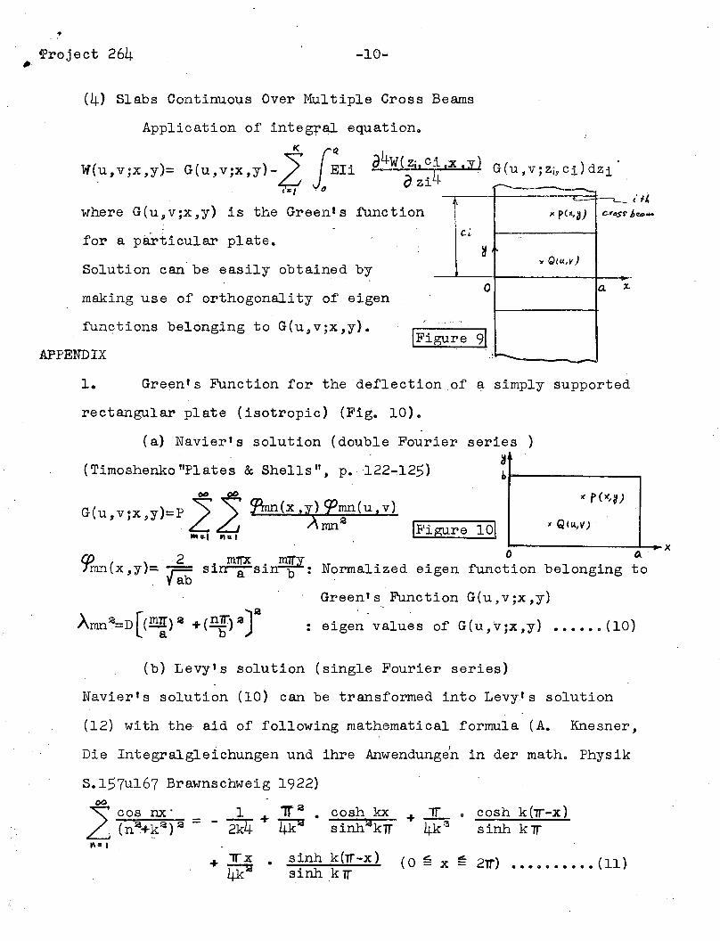
(4) Slabs Continuous Over Multiple Cross Beams

..-...--------~.------c=~

" p(~,a) c.'DSt'

c.~

~'" Q(U,v)

0 a. x.

..............gure 9l

".~~

IFi

making use of orthogonality of eigen

functions belonging to G(u,VjX,y}.

Application of integral equation...

Zl< fq a4W( Zj, ci .x .y) .W(.u,VjX,y)= G(u,v;x,y)- Eli i G(U,VjZi,ci)dzi

ozi4 .<=/ ' ()

where G(u,VjX,y) is the Green's function

for a particular plate.

Solution can'be easily obtained by

APPENDIX

1. Green's Function for the deflection of a simply supported

rectangular plate (isotropic) (Fig. 10).

(a) Navier's solution (double Fourier series)

(Timoshenko "Plates & Shells", p. '122-125)~

~t-------....,

IFigure 10( - QILl/II) .

1----------1._xG) 2 mn. m1Ty 0 D..Tmn(x,y}:..~ sin-a-s~n b : Normalized eigen function belonging to

. yabGreen's Function G(u,v;x,y}

: eigen values of G(u,v;x,y} •••••• (10)

(b) Levy's solution (single Fourier series)

Navier's solution (10) can be transformed into Levy~s solution

(12) with the aid of following mathematical formula (A. Knesner,

Die Integralgleichungen und ihre Anwendungen in der math. Physik

S.157u167 Brawnschweig 1922)

1 + 11" a • cosh kx +.JL.... cosh k (lr-x)- 2k4 4k2 sinh2 k1T 4k <3 sinh k lr

+ lfx •4k2

sinh k(lr-x)sinh krr

(0 ~ x ~ 2rr) .0.0 ..•... (11)

-11-

The following are the results of transformation.

(i) v ~ y

Fa200

LlTGD11 =I

nlf { 1 sinhElCl

1 [Sin~(b-V) sinh nlTy _ nn cosh !!.'[X + __ . a (7 . n b . a a a, sinhn7Tb )

Sl~- a

. hnlrv 1nVVcoshn~ (b-v) _ n~b Sln a JSinnVU

asinnVX

aa a a sinhnrroa

(ii) v ~ y

00 sinh ill!:.Y }Fa2l 1 [ a { . nTf nTr n1T'-3-"'""'::i3 n'Yrbh sln~(b-y) - -(b-y) cos~(b-y)Tf D n sinh~ a a a

k:' a n •••••• (12)

Si~.(b-y) jn'll"" nlTv n7Tb sin!#f(b-V)}' J+ a --!L(b-v)cos~ - :--_"1'nh mrb a a a . h nlTb0,. -a sln -a

2. Green's Function for the deflection of semi-infipite

plate strip (Fig.ll).

r()C/~)

xQ(IA,VJ

0 Q x

IFi'gure Ill.

+00-

3. Green's Function for the deflection of

The solution can be easily derived by making b ~ co in the

Levy's solution (12) derived above.

1 n~b' b 1 nwbnTtb -- mr --b » 0 si~ "'"2 e a , cosh-a-v 2 e a

\~ ± n~ (v-y)

W(u, v;x ,y)= ~~D.2 ~<3 r{l .. n:.( V-y )l e al'l=~ ,

I _mITr } - nTT+ (v+y~ 1f TTV

- \ 1+7 (y+v) e a Jsinnausinn~.n.

(

upper sign for ~y ) ..

],.mver sign for -¢.y

••••• (13)

infinite plate strip.

Since the second series of eq. (13) represents the image of the

first s,eries with respect to x-axis , it is obvious that the first

series is the required solution.

.",.·"pro j ect 264

~~W(u,v;x,y)= 2~DL

~:I

This is the solution

)j.fIIP.~YjY.'

~12-

1 [ ..gjL 1±!?-{-( v-y) mTu nlrxn 3 1+ a (v-y)J e sin--asin--a-

given in (7)

4. Derivation of closed form expressions (9) for ~JIx(u,v;x,y)

My(u,v;x,y) of an infinite plate strip.

In order to sum up the series sollitionfor Mx , My given (d),

the following mathematical formul.a can be applied.

1-1' ~os x 1 l-r2cos nx = 1-2r cosx+1'2 -1 ="2 (1-21'cosx+1' 2 -1) •• (15)

c;osnx = - 1 log (1-21' cos x+1' 2 ) •••••••••••••••• (14)2

for values of lr:1 <1. (Whittaker & Watson t s J:1ode1'n Analysis p.190,

ex.l) •

()O +n TT (v-y) 00 -t!!.!L. (v-y)~ 1 0- _ a sinnml.sinnTfX- 1

2~ 1 ~ a (cosE:..:!L.(u-x)-cosn 71" (u+x»Lnl....- a a Ln~ -aa

~~I ~=I

1 cosh i (v-y)-cosi(u+x')= T:" logLj. cosh -rr (v-y)-cos 1T"(u-x)

a aand 00 -:. -

~ ...nlT (v-y) n1Tu nlTX 1_~±n'JT (v-y) n7T" n71"Le - a si:r:r--a-Sin--a=2LC a (c0s-a(u-x)-cos-a.(u+x»M:' M:/

= 1 t sinhf(v-y) sin~ (v-y) )

4\cosbJI( v-y) -cos1l:(u+x) cosh¥a( v-y) -cos{(u-x)a aTherefore,

MX(U,V;X,y)} ~ [(1+)1) log cosh-f(v-y)-cos-1t-(u+x) +: (l-vl-i-(v-y) XMy(u, v;x, y) = Tf cosh-f( v-y) -cos~(u-x) --

sinhf(v-y)

( cos~(v-y)-cos~(u+x)- sinh-t( v...,y)

- coshf-(v-y) -cos-I-(U-xJ 1.