Influence of Surface Flatness on Bolted Flanges

Bolt Section Method and Fatigue Strength Limit

Ytflathetens Påverkan på Flänsförband

Bolt Section Method och Utmattningshållfasthet

Anders Söderlund

Faculty of Health, Science and Technology

Degree Project for Master of Science in Engineering, Mechanical Engineering

30 HP/ Credit points

Supervisor: Henrik Jackman

Examiner: Jens Bergström

2017-06-20

35106172

Influence of Surface Flatness on Bolted Flanges Strength and Fatigue Strength Limit

ANDERS SÖDERLUND

© ANDERS SÖDERLUND, 2017

Supervisors: Lennart Ekvall & Per Widström, GKN Aerospace Sweden AB Engine Systems

Supervisor: Henrik Jackman, Karlstad University

Master’s Thesis 2017

Faculty of Health, Science and Technology

Division of Mechanical Engineering

Karlstad University

SE-65188 Karlstad

Telephone +46 54 700 1000

Abstract

GKN Aerospace is one of the few main suppliers of engine components in the world,

continuously cultivating engineering and design methods. An important factor in this are the

components ability to withstand fatigue and to provide designs to improve fatigue strength

limit. A design element that occurs in many components construction is the bolted joint,

particularly for circular casings. The conditions for these are also susceptible to fatigue failure.

This report focusses of the surface flatness of bolted joints used in flanges and with the help

of CAE-programs find the best way of modeling the specific problem. The threads in the bolt

and nut are complicated to model accurately. Therefore, some alternative solutions were

evaluated and verified as acceptable. When a proper way to model the thread was found, this

study was focused on investigate the influence of a deviating surfaces on flanges where bolted

joints are applied. Finally, influence on fatigue strength of the bolted joint was studied for

flange surface deviating from nominal. The Bolt Section Method that creates a 2-dimensional

contact surface between the bolt and nut is found to display behavior that resembles that of

thread contact. Results on stiffness, contact and displacement correlate well to the model

where 3-dimensional threads were modelled (True Thread Modeling). It also lower the

computational time significantly and a viable option for Finite Element Analysis on bolted

joints. The surface deviation on the flange results in lower fatigue strength. A surface

deviation also causes plasticity to occur in both bolt and nut by simply pre-loading the joint,

when part of the pretension is used to close the gap. The direction of the surface deviation will

influence as well. When the gap is located at the inner diameter we found the lowest fatigue

life. To detail the flatness requirement, it is required also to account for the effect from prying

bolt, pretension ratio and friction coefficient. The conclusion from this master thesis was that

the modeling of threads can be simplified by implementing the Bolt Section Method. The

influence on fatigue was described by a general model and flatness requirements can be

established accordingly.

Abstrakt

GKN Aerospace är en av de mest framstående leverantörerna av motorkomponenter i världen

och kontinuerligt drivande i ingenjörskap och design. En viktig faktor i detta är en

komponents förmåga att motstå utmattningsbrott och designa för att förbättra

utmattningshållfastheten. En komponent som förekommer i de flesta konstruktioner är

skruvförband och dessa då ofta mottagliga för utmattningsbrott. I rapporten analyseras

flänsförband med hjälp av finita elementmetoden och mjukvaruprogram för att nå de bästa

resultaten från det specifika problemet. Gängorna i bult och mutter är svårmodellerade och

kommer med flertalet ogynnsamma aspekter likt tidskonsumering och elementstorlek som

krävs. I rapporten undersöks hur gängkontakt är implementerat på bästa sätt. När den

optimala modelleringen funnits utfördes en analys av ytflathetens påverkan på ett

skruvförband och slutligen en undersökning hur detta påverkar utmattningshållfastheten på

komponenten. Den undersöka kontaktmetoden för att implementera det mekaniska beteendet

av gängor (Bolt Section Method) konstruerar en tvådimensionell kontaktyta mellan bult och

mutter. Resultaten från denna metod korrelerar väl med modellerade tredimensionella gängor

beträffande styvhet, kontakter och förskjutning. Den erbjuder också omfattande sänkning i

beräkningstid eftersom modellen kräver betydligt färre element för att nå konvergens. En

lutande yta på flänsar resulterar i sänkt utmattningshållfasthet och plasticering redan under

förlastning av skruvförbandet. Det noterades också hur riktningen på lutningen influerar på

olika sätt, att ett orsakat gap vid livet sänker utmattningshållfastheten ytterligare i jämförelse

med ett gap i änden av flänsen.

Preface

This report is the result of a master thesis conducted at the master degree program in material

science, Karlstad University. The thesis was supervised and accomplished in collaboration

with GKN Aerospace AB in Trollhättan, Sweden during the spring of 2017.

Extended gratitude to the supervisors from GKN Aerospace AB, Per Widström and Lennart

Ekvall. Without their invaluable guidance, this thesis would never have been completed.

Further thanks to the supervisor from Karlstad University, Henrik Jackman.

Nomenclature

Abbreviations

FE Finite Element

FEA Finite Element Analysis

BSM Bolt Section Method

MPC Multiple Point Constraints

TTM True Thread Modeling

GAS GKN Aerospace AB

CAD Computer Aided Design

FSL Fatigue Strength Limit

CPU Central Processing Unit

1

Contents

1. Introduction ............................................................................................................................................... 1

1.1 GKN Aerospace AB ........................................................................................................................ 1

1.2 Problem statement .......................................................................................................................... 2

1.3 Purpose ............................................................................................................................................... 2

1.4 Aim ....................................................................................................................................................... 3

1.5 Computer-Aided Engineering (CAE) ....................................................................................... 3

1.6 Background ....................................................................................................................................... 4

1.6.1 Bolt .............................................................................................................................................. 4

1.6.2 Bolt Design ............................................................................................................................... 7

1.6.3 Nut ............................................................................................................................................... 7

1.6.4 Bolted Joints ............................................................................................................................. 8

2. Theory ......................................................................................................................................................... 9

2.1 Analytical calculation ..................................................................................................................... 9

2.1.1 Pre-tension................................................................................................................................ 9

2.1.2 Tensile load ............................................................................................................................ 12

2.1.3 Bending Moment .................................................................................................................. 13

2.1.4 Fatigue ..................................................................................................................................... 14

3. Finite Element Theory ......................................................................................................................... 17

3.1 Contacts ....................................................................................................................................... 17

3.2 Theory: Bolt Section method ................................................................................................ 19

3.3 APDL ............................................................................................................................................ 20

3.4 Mesh .............................................................................................................................................. 20

3.5 Material ........................................................................................................................................ 22

3.6 Element type............................................................................................................................... 24

3.7 Loads and Boundary Conditions .......................................................................................... 25

4. Finite Element Analysis ....................................................................................................................... 26

4.1 Contact Evaluation ....................................................................................................................... 26

4.2 Method Evaluation ....................................................................................................................... 28

4.3 Tensile Test Comparison ............................................................................................................ 31

4.4 Surface deviation ............................................................................................................................ 34

5. Results ....................................................................................................................................................... 39

5.1 Contact Method Evaluation ....................................................................................................... 39

5.2 Method Evaluation ....................................................................................................................... 41

5.3 Tensile test ...................................................................................................................................... 49

2

5.4 Surface Deviation .......................................................................................................................... 53

6. Discussion ................................................................................................................................................. 69

6.1 Analysis of the Bolt Section Method ....................................................................................... 69

6.2 Method Evaluation ....................................................................................................................... 72

6.3 Tensile Test Comparison ............................................................................................................ 73

6.4 Surface Deviation .......................................................................................................................... 74

7. Conclusion ................................................................................................................................................ 77

7.1 BSM ................................................................................................................................................... 77

7.2 Surface influence on fatigue strength limit ........................................................................... 77

7.3 Tolerances ....................................................................................................................................... 77

8. Future Work............................................................................................................................................ 78

8.1 Bolt Section Method ..................................................................................................................... 78

8.2 Method Evaluation ....................................................................................................................... 79

8.3 Tensile Test Comparison ............................................................................................................ 79

8.4 Surface Deviation .......................................................................................................................... 79

References ......................................................................................................................................................... 81

1

1. Introduction

The master thesis was executed at GKN Aerospace Sweden AB in Trollhättan. This chapter

have the function of declaring the purpose, aim, objective and some theoretical background of

the master thesis. Also, give a summary of the company that is GKN and more specifically on

GKN Aerospace AB.

1.1 GKN Aerospace AB

GKN is a global engineering business. GKN Group consists of four different division;

Aerospace, Driveline, Land Systems and Powder Metallurgy. Facilities can be found in over

30 countries with a total of 56100 employees, where the Aerospace group is responsible for

16700 of these [1]. The Aerospace group are active in 14 countries and accounts for 33 % of

the total revenue, placing it in second place, 13 percentage points below Driveline but around

three times larger than the other two divisions. The manufacturing of aerospace products are

both for commercial and military purposes, where three quarters correspond to the

commercial applications and the rest to military applications [1]. The facility where the

master thesis has been conducted, in Trollhättan, is a part of the aerospace division and in

turn a sub-division focusing on Engine systems. The Engine systems sub-division also have

facilities in Mexico, Norway and the United States of America. In Trollhättan there are both

commercial-, military-, and space components handled and in addition to that also fractions

concentrating on engine service and maintenance.

Specific components that are designed, manufactured or both are displayed in Figure 1.1.

Figure 1.1: Showing the engine components designed and/or manufactured at GAS in Trollhättan [1].

2

1.2 Problem statement

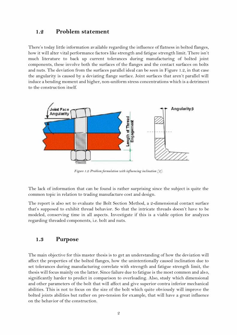
There’s today little information available regarding the influence of flatness in bolted flanges,

how it will alter vital performance factors like strength and fatigue strength limit. There isn’t

much literature to back up current tolerances during manufacturing of bolted joint

components, these involve both the surfaces of the flanges and the contact surfaces on bolts

and nuts. The deviation from the surfaces parallel ideal can be seen in Figure 1.2, in that case

the angularity is caused by a deviating flange surface. Joint surfaces that aren’t parallel will

induce a bending moment and higher, non-uniform stress concentrations which is a detriment

to the construction itself.

Figure 1.2: Problem formulation with influencing inclination [2].

The lack of information that can be found is rather surprising since the subject is quite the

common topic in relation to trading manufacture cost and design.

The report is also set to evaluate the Bolt Section Method, a 2-dimensional contact surface

that’s supposed to exhibit thread behavior. So that the intricate threads doesn’t have to be

modeled, conserving time in all aspects. Investigate if this is a viable option for analyzes

regarding threaded components, i.e. bolt and nuts.

1.3 Purpose

The main objective for this master thesis is to get an understanding of how the deviation will

affect the properties of the bolted flanges, how the unintentionally caused inclination due to

set tolerances during manufacturing correlate with strength and fatigue strength limit, the

thesis will focus mainly on the latter. Since failure due to fatigue is the most common and also,

significantly harder to predict in comparison to overloading. Also, study which dimensional

and other parameters of the bolt that will affect and give superior contra inferior mechanical

abilities. This is not to focus on the size of the bolt which quite obviously will improve the

bolted joints abilities but rather on pre-tension for example, that will have a great influence

on the behavior of the construction.

3

To analyze the possibilities to perform finite element analysis on bolted joints and investigate

the options to simulate threaded contact and give advantages versus disadvantages to be able

to acquire the correct influence of threads.

1.4 Aim

That through simulation in computer-aided engineering programs (CAE) using finite element

methods and a comparison to a practical test to evaluate the correlation between deviations

on the flange and strength and fatigue strength limit of the bolted flanges. Optimizing the

flatness of the flange, to determine if current tolerances are relevant or if they need to be

lowered to decrease production costs or if better and higher tolerances are needed to increase

mechanical abilities of the component despite manufacturing cost increase due to this. This

regard each separate component in the assembly, including: bolt, nut and flanges.

To establish whether the bolt section method is viable in finite element analysis.

1.5 Computer-Aided Engineering (CAE)

During this master thesis second part, where the problem is to be evaluated with finite element

analysis (FEA) by computer software, two main CAE-programs are used, Hypermesh and

Ansys. Hypermesh is a multidisciplinary finite element pre-processor that usually starts with

an imported Computer aided design-file (CAD) to later be exported as a ready-to-go solver

file. The ability to handle advanced geometries and meshing capabilities provide a good

environment for rapid model generation. Ansys will purely be used as a solver of the input file

earlier created in Hypermesh and to evaluate and study the simulation HyperView is used

instead of Ansys since it’s easier to get the valuable data needed in this case. Also, Ansys

include the bolt section method (BSM), which the thesis will investigate, evaluate and validate

for thread analysis.

4

1.6 Background

A short explanation of different components, their purpose, general history and design with

advantages and disadvantages.

1.6.1 Bolt

The distinction between a bolt and a screw is unclear and commonly misunderstood. There

are several practical differences, but these practical differences also have an overlap between

bolts and screws to some extent. The defining distinction, per Machinery’s Handbook [8] is

in their intended purpose. Bolts are for the assembly of two unthreaded components, with aid

of a nut, creating a bolted joint. Screws in contrast are used with components, where at least

one of the components have its own internal thread, which even may be formed by the

installation of the screw itself. Many threaded fasteners can be described as either-or bolts,

depending on how they are used.

Bolts are often used in bolted joints, which the name clearly implies. This is a combination of

the nut applying an axial clamping force and also the shank that’s acting as a dowel, pinning

the joint against sideways shear forces. For this reason, many bolts have plain unthreaded

shank that’s also known as the grip length, as this makes for a better, stronger dowel. The

presence of the unthreaded shank has often been given as characteristics of bolt versus screws,

but this is incidental to its use, rather than defining [4].

Where a fastener that forms its own thread in the component when being fastened is called a

screw. This is most obviously so when the thread is tapered (i.e. traditional wood screws for

example), precluding the use of a nut, or when a sheet metal screw or other thread-forming

screw is used.

A screw must always be turned to assemble the joint. Many bolts are held fixed in place during

assembly, either by a tool or by a design of non-rotating bolt, such as a carriage bolt, and only

the corresponding nut is turned.

In the specific bolted flanges that are designed and constructed at GAS the 12-point type is

utilized.

A 12-point head is a combination of two overlapped hexagon shapes. Standard 12-point hex

socket bits and wrenches fit these screws or bolts. The heads are typically flanged and fit

standard Allen hex socket cap screw counterbores. Advantages of these include higher torque

capability compared to Allen hex socket, and lack of a recess to trap water [5]. A disadvantage

is the higher cost of production to manufacture this head. The higher strength and larger

bearing area under the head of this design provide additional benefits for assemblies over

standard hex caps. Clamp load for engine applications are typically higher than most others,

which make a 12-point will help to provide.

There are several important dimensional attributes of a bolt that will influence the mechanical

abilities in a bolted joint. These can be seen and described respectively by Figure 1.3 and Table

1-1.

5

Figure 1.3: Important bolt dimension [3].

Clarification of indexation in Figure 1.3 are found in Table 1-1.

Table 1-1: Explanation of index in Figure 1.3

Index Dimension

B Bolt Diameter

C Width Across Corners

D Bolt Head Diameter

F Width Across Flats

H Head Height

L Length of Bolt

LB Shank Length

LT Thread Length

T Height of Gaging Ring

W Height of 12-point

X Chamfer or Radius

Y Transition thread Length

The specific type of bolt and nut at GAS is specially designed for aerospace and space

applications. The bolt material is INCO and the material of the nut is Waspaloy. INCO is a

family of austenitic nickel-chromium-based superalloys and the limiting chemical

composition can be found in Table 1-2.

6

Table 1-2. Limiting chemical composition of the INCO-material [23]

Element Limiting Chemical Composition (%)

Nickel (plus Cobalt) 50-55

Chromium 17-21 Iron Balance Niobium (plus Tantalum) 4.75-5.50

Molybdenum 2.80-3.30

Titanium 0.65-1.15

Aluminum 0.20-0.80 Cobalt 1.00 max Carbon 0.08 max

Manganese 0.35 max

Silicon 0.35 max

Phosphorus 0.015 max Sulfur 0.015 max Boron 0.006 max

Copper 0.30 max

Waspaloy are trademarked by United Technologies Corp and is an age hardened austenitic

nickel-based superalloy with a face-centered-cubic structure. The main advantage with using

Waspaloy is its thermal stability, it exhibits excellent strength attributes up to a temperature

of 980 °C. This is crucial since the conditions during application reach around 500 °C, where

numerous materials would suffer greatly in regards to strength. Additional positive aspects

being good corrosion resistance and oxidation resistance which makes it useful in though

conditions, such as gas turbines. [5]

Chemical composition maximum and minimum of the Waspaloy can be found in Table 1-3

and the nominal composition in Table 1-4.

Table 1-3. Possible chemical composition of the Waspaloy [5]

Cr Ni Mo Co Al Ti B C Zr Fe Mn Si P S Cu

MIN 18.00 -- 3.50 12.00 1.20 2.75 0.003 0.02 0.02 -- -- -- -- -- --

MAX 21.00 Balance 5.00 15.00 1.60 3.25 0.01 0.10 0.08 2.00 0.10 0.15 0.015 0.015 0.10

Table 1-4: Nominal composition of Waspaloy nuts [5]

Element Percent by Weight

Nickel 58 % Chromium 19 %

Cobalt 13 %

Molybdenum 4 %

Titanium 3 %

Aluminum 1.4 %

7

1.6.2 Bolt Design

Standard practice of aerospace applications is to use reduced shank, double hex head bolts (12-

point bolt). The reduced shanks are preferable to reduce the axial flexibility ratio. The

temperature needs to be considered for the choice of bolt material regarding limitation and

applicability. Size is also something that has to be taken into account, bolts smaller than 6.35

mm (1/4-inch) are easily fractured during assembly or disassembly, but a smaller bolt size

will minimize the weight of the bolted joint and is sought. Notable is also that in aerospace

applications, dimensions still occur only in imperial units to go with an American standard

[6]. A larger number of smaller bolts will always yield the lightest joint configuration this

due to that reduction of flange height required to provide seating surface for the fastener.

The thesis will first and foremost evaluate the specific size used in the current application and

its SI-unit counterpart. These are the quarter inch bolt and M6 bolt.

1.6.3 Nut

There are self-aligning nuts, constructed for the specific purpose of handling a deviation at on

the joint surface. Most usually used in aerospace application that is the case for GAS and even

more specific to the Waspaloy nuts that will be examined later in this thesis. These self-

aligning nuts are made out of two components, a nut with a convex base which will fit a

washer. Necessary when the two surfaces of the assembly aren’t parallel. These nuts are

supposed to be able to handle a surface deviation reaching around 5°. They are used in

aerospace application, however they’re also expensive and adds weight to the construction.

Weight reduction being one of the most sought abilities during construction making the usage

of this nuts only when it’s a must. The design of the self-aligning nut is displayed in Figure

1.4.

Figure 1.4: Displays how a self-aligning nut treats the surface inclination [7].

8

The thesis will not go in to the specifics of self-align nuts, but that these exists in the realm

of aerospace engineering vouch for the problems that is around surface flatness for bolted

joints.

1.6.4 Bolted Joints

One of the most common elements used in construction, whether it’s in construction of

transportation vehicles or any other applied area. They consist of fasteners, in this case the

fasteners are composed of one bolt and one nut. There are two different practices of bolted

joints, one is designed for tension and the other for shear load. The bolt and nut earlier

mentioned are representatives from the family designed to withstand tension. The thesis will

not be handle the bolted joint sub-group that handles shear, but tension will be investigated

further.

9

2. Theory

This chapter’s purpose is to describe how and why specific methods were chosen to attain

relevant results. This regarding the literature survey, analytical calculations and

Hypermesh/Ansys/HyperView simulations.

2.1 Analytical calculation

There’s no direct way of calculating the influence of a surface deviation on fatigue strength of

a bolted flange. That’s the major reason for the GAS interest in performing the investigation

in the first place, the lack of actual knowledge around it.

As said, no direct way of calculating the influence of a surface deviation, no equation where

input parameters can provide a result of for example changed fatigue strength limit. Also, a

general lack of information surrounding the problem. Worrying, since bolted joints can be

found in so many constructions and that there are tolerances put on both flange and bolt head

surfaces, allowing surfaces with deviations without the effect of it. By having tolerances,

perspective is that it’s fine for the surface to deviate to some extent, without being considered

unreliable after manufacturing of the component. The few sources that try to explain the

phenomenon tells a story of a significant drop in life expectancy when the surfaces deviate

from each other and extremely when passing above 2° [2]. This is from the ideal parallel

alignment that is sought. The problem with a deviating surface is also seen through the

counter measures that are against it described in section 1.6.3.

Analytical calculations will have to investigate several different types of loadings and in turn

several elemental cases surrounding bending, shear, tensile and rotational stresses and strains

in more simplistic ways.

2.1.1 Pre-tension

For a bolted joint to function correctly, a preload or pre-tension is needed to make sure it

withstands large mechanical loads or cyclic loads under an extensive time period. It is

important for the joint in several aspects and as an example prohibits the nut from loosen itself

during vibrations, thermomechanical loads etc. There are several different ways of controlling

the tightening of the joint, most common methods include Torque controlled tightening,

angle-controlled tightening and yield-controlled tightening. If the greatest possible assembly

preload is sought, yield-controlled tightening should be chosen [11]. Torque-controlled

tightening is the widespread technique on account of its simplicity and cost-effective tools. A

correctly preloaded bolted joint (i.e. high preload) will improve mechanical properties in every

single way. A correctly applied preload will cause 80-90 % of external loading to go through

the substrate rather than the bolt, however this percentage may fluctuate due to differences

in stiffness [17].

There are several types of methods to achieve this pre-load that will improve the mechanical

abilities of the joint, the complexity and accuracy of these vary in a quite broad spectrum.

10

Table 2-1 shows the method of pre-loading the bolted joint and the inaccuracy of correctly

applied pre-tension each of these [8].

Table 2-1. Methods of pre-loading and their inaccuracy [8]

Method Inaccuracy (± %) Torque wrench on unlubricated bolts 35

Torque wrench on cad plated bolts 30

Torque wrench on lubricated bolts 25

Preload indicating washer 10 Strain gauges 1 Computer-controlled wrench (below yield) 15

Computer-controlled wrench (yield sensing) 8

Bolt elongation 5

Ultrasonic sensing 5

It should be noted that the distribution of the torque under normal circumstances is in that

way that 50 % will be lost due to friction against abutment surfaces. 40 % will be lost through

friction in the threads and the remaining 10 % is what will be the actual pre-load [17]. This

may vary though, in some cases the percentage that goes to pre-load can reach 30 %.

The preloading of the component will depend on several parameters surrounding the bolt and

to calculate the torque needed to achieve the sought pre-tension.

The calculations on the desired torque is given by Fel! Hittar inte referenskälla.-4 and Table

1-1: Explanation of index in Figure 1.3 [11]:

3

1

10***

1

ss

FM

F

V APd

F

Sk

KM (1)

Pd

DdK uk

2

*'tan2 (2)

2

221 *155.112

1

d

P

Dk g

As

(3)

s

As

AD

4 (4)

11

Table 2-2. Parameters in Fel! Hittar inte referenskälla.-4 [11]

Index Material property (Unit)

MV Torque (Nm)

K Factor

k1 Correlation between effective stress and tensile stress

SF Distribution of pre-load

FFM Average pre-load (N) d Diameter of the bolt thread P Thread pitch diameter

As Tension area cross section, (mm2)

σs General indexation for Rp0.2 (N/mm2)

Rp0.2 Extension limit (N/mm2) Rel Lower yield limit (N/mm2)

ϧ Thread pitch angle (°)

d2 Average diameter of the bolt thread

ρ’ Friction angle of thread

Dk Plant surface friction diameter (mm)

μu Friction coefficient of the plant surface

μtot Active friction coefficient in torque-force exchange

σe Effective stress

σF Pre-tension of the bolt

AsD Diameter of the tension-area

P Thread pitch (mm)

μg Coefficient of friction in the thread

d2 Bolt threads average diameter

Fel! Hittar inte referenskälla.-4 and the sheer number of influencing parameters from Table

2-2 shows how intricate and complex it is to evaluate the torque needed to achieve the desired

pre-tension. That in turn explain the varying accuracy results that usually is when preloading

from Table 2-1. Also, including the basic problem of evaluating relevant parameters as friction

that is dependent on so many variables in itself. So, one of the most significant parameters to

achieve functional bolted joints relies on numerous factors and has to be handled carefully,

especially in this report.

12

2.1.2 Tensile load

The main type of load exerted on bolted joints and most common for bolts to be designed to

withstand. By clamping together two or more components a tensile stress is exerted on the

bolt which then increase when the two (or more) components try to separate. If a proper pre-

tension is applied, most of the load will go through the substrate instead of the bolts.

Therefore, part of the tensile stress is no major problem, since pre-tension is advantageous for

the joint, it is all well for the joint to be exerted to some extent of tensile stress. But this stress

should be through the preloading and nothing else. Although, high tensile stress will as

imagined lead to failure, therefore it’s often sought to get a pre-tension set to in an around the

yield stress because after that the bolt is deformed and weakened. In the present problem that

is the thesis main ambition to assess, the tensile stresses will be represented by the flanges the

bolt components is set to hold together. This is displayed in Figure 2.1, where the bolt and

nut can be seen on the far left and right. The two central components are representative of

the flanges that the joint itself seeks to hold together.

Figure 2.1: Simple explanation of the tensile load applied a bolted flange [14].

Figure 2.1 is representative of the ultimate problem that is sought to be investigated and when

external forces try to separate the flanges there will be tensile stresses exerted on the bolted

joint.

13

2.1.3 Bending Moment

In an ideal environment, a bolted joint and bolt in particular is not exerted to a bending

moment, but this is very rarely the case. Due to that the flange can’t be considered as

completely rigid or tolerances on surface flatness as examples. Problems occur when the

surfaces are not completely flat, then by preloading the element a bending moment will be

induced due to the inclination on one or both of the surfaces. This will of course increase even

more when the load the bolt is supposed to withstand is applied. The normal force from the

flanges will always be perpendicular to the surface itself and with a deviating surface, the

normal force be perpendicular to the surface but not in line with the axial direction of the bolt

(from pre-tension as an example). This will directly induce stress concentrations that are

inhomogeneous and become especially notable at sensitive points where there’s phases on the

bolt, lowering the life expectancy of the joint straight away. This will be extensively examined

in this thesis and the bending is displayed in Figure 2.2.

Figure 2.2: Displays the moment that occurs when there’s an angularity on the surface [15].

14

2.1.4 Fatigue

Most component failures in application today is due to fatigue, this occurs since it’s harder to evaluate the fatigue strength limit and also harder to examine if the failure is bound to occur. Statistics show that majority of service failures in aircraft components occur by fatigue and it amounts to about 60% of the total failures [10]. Also, the influence of a bending moment is likely to have a significant effect, this since bending induces higher stress levels than the tensile load. An example of this could be found by comparing machines that are set to evaluate fatigue failure, structures that investigate the influence of bending does not need to apply as high load to achieved the stress levels that are to be examined. The bending moment mentioned in this chapter will be instrumental in the latter fatigue failure. Tensile stresses will of course also influence the fatigue strength limit but the major cause for fatigue failure for bolts and bolted joints will likely come through bending fatigue. A small degree of inclination may not be worrying in regards of strength but will most likely

have a large influence on the life expectancy on the components/joints i.e. fatigue strength

limit.

The report will judge the fatigue strength limit according to Basquin’s law. There are several

models to accommodate fatigue life and fatigue crack growth and in aerospace applications

fatigue is dominated by fatigue crack initiation. Then it’s common to utilize the stress-life (SN)

curves accordingly to Basquin’s law. There are also numerous empirical models to

accommodate for large scale plasticity, but since this generally isn’t the case in aerospace it’s

considered unnecessary. Basquin’s law assess the varying amplitude cycling and the effect of

the maximum stress level. Basquin’s law is described in Fel! Hittar inte referenskälla..

CN a

f (5)

Description of the parameters used in Basquin’s’ law (Fel! Hittar inte referenskälla.) is

explained in Table 2-3.Fel! Hittar inte referenskälla.

Table 2-3: Describes the parameters that are used in equation 5.

Indexation Parameter Unit

Stress amplitude MPa

Nf Number of cycles - a (1/a=m) Empirical constant -

C Empirical constant that describes the maximum completely reversing stress.

MPa

Reconfiguring Fel! Hittar inte referenskälla. to solve for Nf since it’s the unknown quantity

in this case gives:

15

m

f

a

f

a

C

N

f

f

a

f

a

f

CN

CN

eeea

CN

CNa

CNCN

f

1

1ln

ln*

1*lnln

lnln*

m

f

CN

(6)

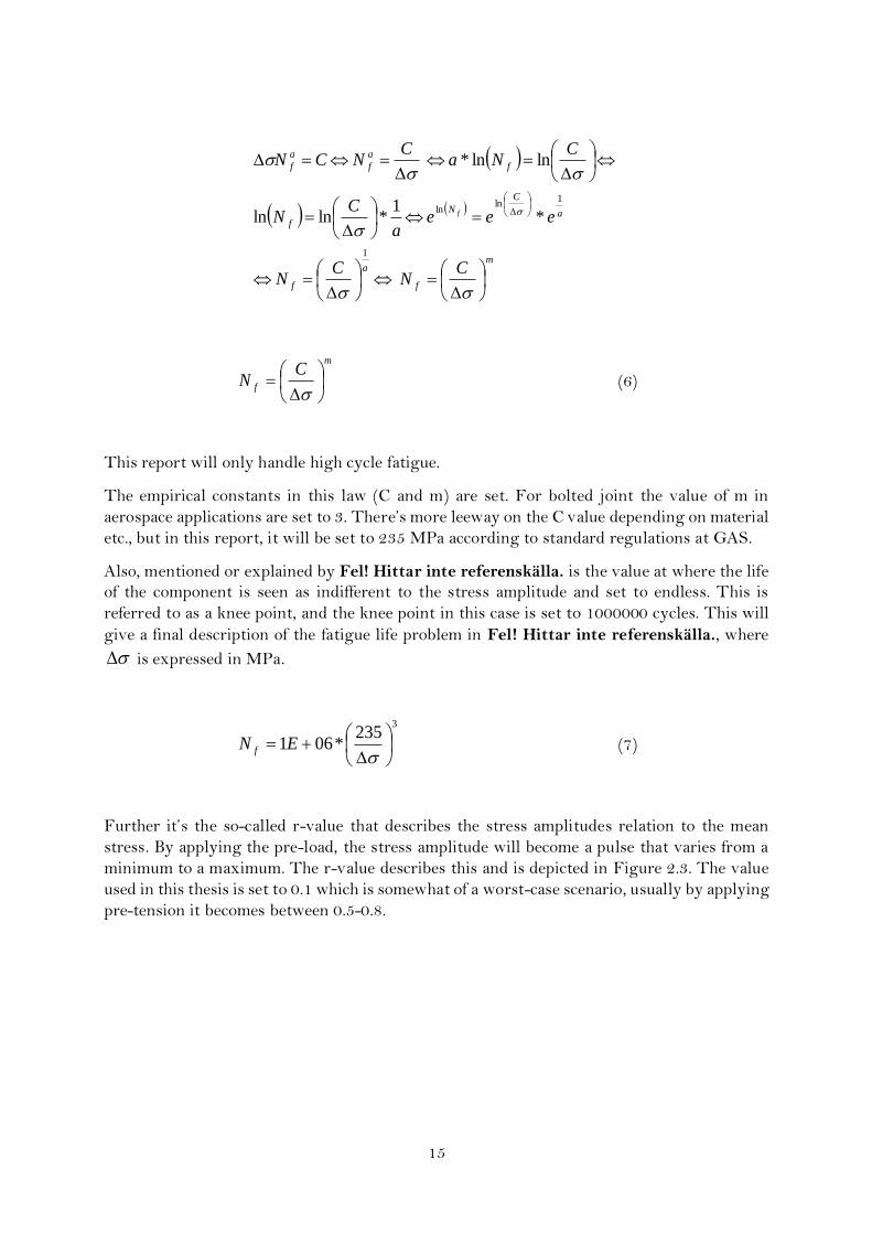
This report will only handle high cycle fatigue.

The empirical constants in this law (C and m) are set. For bolted joint the value of m in

aerospace applications are set to 3. There’s more leeway on the C value depending on material

etc., but in this report, it will be set to 235 MPa according to standard regulations at GAS.

Also, mentioned or explained by Fel! Hittar inte referenskälla. is the value at where the life

of the component is seen as indifferent to the stress amplitude and set to endless. This is

referred to as a knee point, and the knee point in this case is set to 1000000 cycles. This will

give a final description of the fatigue life problem in Fel! Hittar inte referenskälla., where

is expressed in MPa.

3235

*061

EN f (7)

Further it’s the so-called r-value that describes the stress amplitudes relation to the mean

stress. By applying the pre-load, the stress amplitude will become a pulse that varies from a

minimum to a maximum. The r-value describes this and is depicted in Figure 2.3. The value

used in this thesis is set to 0.1 which is somewhat of a worst-case scenario, usually by applying

pre-tension it becomes between 0.5-0.8.

16

Figure 2.3. Depicts how the r-value influences the stress amplitude.

This is needed when the stress amplitude is to be calculated, the minimum and maximum

stress will be interpolated from the results at a certain external load applied. The stress

amplitude is easily calculated after that, this described by Fel! Hittar inte referenskälla..

2

minmax

amp (8)

17

3. Finite Element Theory

The major part of the thesis was performed with the help of CAE and this chapter describes

how the solutions are evaluated and explain why these methods were chosen.

3.1 Contacts

During the FEAs and comparisons between Multiple Point Constraint (MPC), Bolt Section

Method (BSM) and True Thread Modeling (TTM) contacts are defined. Of the two surfaces

in contact, one of them is once defined as the master surface and the other as the slave. The

same regards to the thread contact explained in 3.2 Theory: Bolt Section method. This

constitutes that constraints can be set and penetration prohibited. Thereby, removing the risk

of the unrealistic behavior in the form of two bodies overlapping into each other.

Then the contact has to be constituted how to behave and interact further. There are several

types of contact types to choose between but the main two being considered for the latter

FEAs are kinematic contact method and penalty contact method.

MPC contact is somewhat investigated, but never as a solution for the final analysis. The

MPC utilizes bonded means. Bonded contact is a linear connection. A linear penalty-based

contact connection between two bodies are defined by a contact surface of the face of one body

and target surface on the face of the other body (master/slave). The contact and target

elements lies on the peripheral surface of the solid elements.

Penalty contact method have no problems or conflicts due to other constraints applied.

Basically, adding a term acting like a stiff spring and lets one surface slightly penetrate the

other surface before being exerted to a “spring” forcing it back. This is done by adding a term

that’s zero when no constraints are violated and non-zero when constraints are violated.

Otherwise the kinematic contact method is used which utilizes the Lagrange multiplier

method, adding a term that equals 0 when in contact. Positives with this contact method is

the accuracy which is better than the penalty contact method. But then again, it’s a way more

sensitive method to use in contacts. The computational cost may become very high and there’s

a risk of the computations to diverge instead of converging, leaving the analysis without any

results. These methods advantages and disadvantages are displayed in Table 3-1. The +/-

indicates advantages and disadvantages respectively, no indicator is general information.

18

Table 3-1: Contact methods and information on advantages and disadvantages using them [18]

Pure Penalty Augmented Lagrange Normal Lagrange MPC

+ Good convergence behavior (few equilibrium equations)

- May require additional equilibrium iterations if penetration is too large

- May require additional equilibrium iterations if chattering is too large

+ Good convergence behavior (few equilibrium iterations)

- Sensitive to selection of normal contact stiffness

Less sensitive to selection of normal contact stiffness

+ No normal contact stiffness required

+ No normal contact stiffness is required

- Contact penetration is present and uncontrolled

Contact penetration is present but controlled to some degree

+ Usually, penetration is near-zero

+ No penetration

+ Useful for any type of contact behavior

+ Useful for any type of contact behavior

+ Useful for any type of contact behavior

- Only bonded and No separation behaviors

+ Either iterative or direct solvers can be used

+ Either iterative or direct solvers can be used

- Only direct solver can be used

+ Either iterative or direct solvers can be used

+ Symmetric or asymmetric contact available

+ symmetric or asymmetric contact available

Asymmetric contact only

Asymmetric contact only

+ Contact detection at integration points

+ contact detection at integration points

Contact detection at nodes

Contact detection at nodes

For this thesis, the kinematic contact method has been chosen, the contacts are considered to

have an important influence when the surfaces in contact deviate. Therefore, the more accurate

and less computational effective Normal Lagrange multiplier method will be more

appropriate.

19

3.2 Theory: Bolt Section method

The Bolt Section Method is a way to perform a simplified bolt thread modeling without the

unpractical refined mesh discretization needed on both bolt and bolt hole during True Thread

Modeling (TTM) to achieve convergence. Ansys have made it possible to accomplish the

behavior of threads through contact elements instead of complicated modeling and fine mesh

size that will greatly increase computational time. All this through contact elements

“CONTA171-175” that they claim have nearly the accuracy of true threaded bolt models [12].

The technique is available both for two-dimensional axisymmetric and three-dimensional

models by simply modeling a smooth cylindrical surface on both bolt and hole. The user

specifies the geometry of the threads and the end points, the parameters that’s specified are

displayed in Figure 3.1.

Figure 3.1: Bolt parameters used in the BSM contact method [12].

The input parameters include mean pitch diameter (dr), pitch, thread angle (2α), and end points

of the bolt axis ((x2, y2, z2), (x1, y1, z1)). Only referrals to ANSYS Mechanical APDL Contact

Technology and a workshop regarding Ansys Workbench which provides very little

information. [12, 13]

20

3.3 APDL

During all FEAs, APDL (ANSYS Parametric Design Language) is used to evaluate the model

rather than the Ansys-workbench. The Ansys-workbench do have a good and very user-

friendly interface property but there’s an uncertainty regarding some default values. The

workbench sets some default values that’s not displayed and described for the user and this

could in some cases lead to inaccurate models and give a deceptive analysis of the problem

itself. The target is heavily set to converge, and to be able to do this the program may go a

long way in the expense of what could be considered a good analysis. Therefore, ADPL-files

is used, to have complete control and knowledge of what is done during the simulation, leaving

the uncertainty outside of analysis. The ADPL-files basically consist of text files where

programming is done to later on tell the solver (Ansys) what needs and should be done.

The most notable disadvantage with using APDL will most likely appear when the surface

deviation is to be studied. In Ansys classic each and every model (with varying degree of

surface inclination) will have to be constructed and meshed separately. The workbench option

would provide the user with possibility to set the deviation as a parameter and automatically

remesh and vary this. This would make it possible to perform a greater number of analyses

but also give less control over element properties that could become a worry since there’s a

contact between the two flanges.

The difference depends on what’s sought to be done, for speed there is arguments for

workbench and for detail Classic (APDL)

3.4 Mesh

The meshing of the model is significant in many ways for the latter analysis since creating the

elements will influence important FEA factors. First and foremost, creating elements that are

too big will cause to either give a completely deceptive solution to the analysis both regarding

contact, stress concentrations and displacements. It may even cause the computation to

diverge and no solution at all will be reached. Neither will extremely small elements have a

beneficial effect on the analysis, small elements may prompt better results (i.e. contacts, stress

concentrations, displacement values) but will increase computational time. The relation

between the number of nodes and computational is not linear, the nodes are set in a matrix to

be solve, for example doubling the number of nodes would increase the computational time by

a factor larger than two [19]. So, on one side of the spectrum the solution will never be

reached due to collapsing calculation and on the other side the solution will never be reached

since the computation will never be done. An optimization is sought where the mesh provides

an adequate result without taking too much time. Adequate result conclusion may be drawn

after a comparison to a practical test for example. This is why it’s useful to have mesh that

varies depending on the part of the component that’s to be analyzed. Areas where there are

larger stress concentrations for example, can be made finer for a better result and areas

unaffected by the load, moment applied or insipid to the analysis can be rougher (larger). This

will give a better analysis of the problem and have a better computational time than if the

whole component was meshed to a finer state. Complication may occur during this kind of

meshing if the change in size of the elements increase too sudden and give elements that aren’t

21

at all appropriate for a deformation. Problems that might occur is skewed and disproportionate

elements that gives a misleading result of the stress state as an example.

Especially with an element size that differ depending on locations on the component, then all

elements can’t be uniform. Depending on what type of element is chosen, you seek angles

within the element borders to be as alike as possible. Elements that look greatly deformed

before the analysis have a higher tendency to cause problem, a problem could be hourglassing.

Hourglassing results from the excitation of zero-energy degrees of freedom and expresses

itself in reduced integration with too few gauss points, this may be prohibited with full

integration that involve more gauss points. Elements become skewed and two elements

together form something that looks like an hourglass. This is displayed in Figure 3.2.

Figure 3.2. Depiction of hourglass formation.

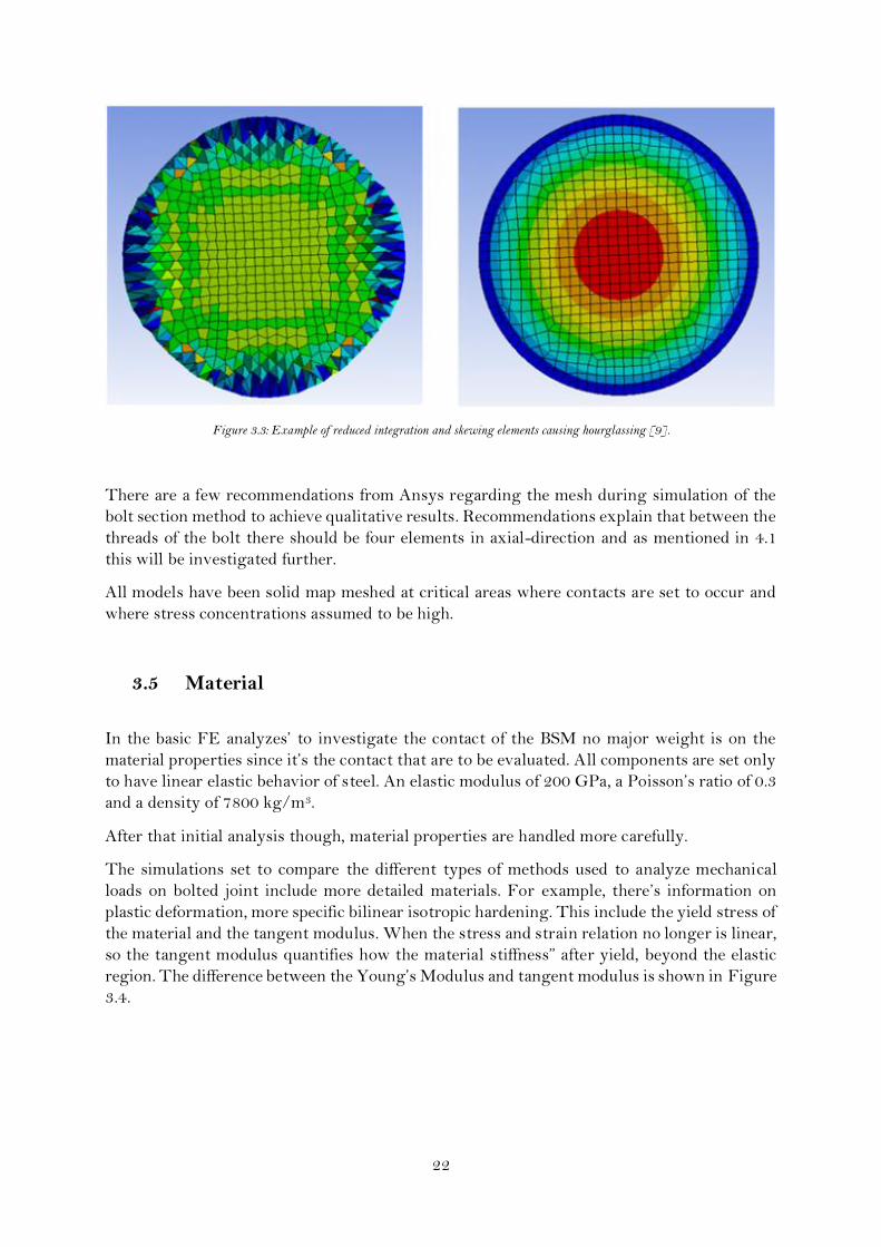
Figure 3.3 clearly depicts how these hourglass formations may give a misleading visualization

of stress concentrations or displacements. These sort of problems is usually more prone to

occur where triangular, tetrahedral or pyramid elements, but as earlier mentioned it might be

necessary for changing element sizes. So, they need to be placed strategically, away from large

deformation or the problem in the left picture in Figure 3.3 will occur. There are other ways

of getting around some of these problems with for example hourglass control to prevent the

hourglass formations, even though it might exploit other problems within the model. System

energy can be artificially removed if hourglass control is applied incorrectly.

All elements that are involved in a contact are configured to be hexagonal elements in shape,

leaving the rest to have a tetrahedral shape. The element size in the contact to simulate threads

are set to become eight per thread as explained in 3.2.

22

Figure 3.3: Example of reduced integration and skewing elements causing hourglassing [9].

There are a few recommendations from Ansys regarding the mesh during simulation of the

bolt section method to achieve qualitative results. Recommendations explain that between the

threads of the bolt there should be four elements in axial-direction and as mentioned in 4.1

this will be investigated further.

All models have been solid map meshed at critical areas where contacts are set to occur and

where stress concentrations assumed to be high.

3.5 Material

In the basic FE analyzes’ to investigate the contact of the BSM no major weight is on the

material properties since it’s the contact that are to be evaluated. All components are set only

to have linear elastic behavior of steel. An elastic modulus of 200 GPa, a Poisson’s ratio of 0.3

and a density of 7800 kg/m3.

After that initial analysis though, material properties are handled more carefully.

The simulations set to compare the different types of methods used to analyze mechanical

loads on bolted joint include more detailed materials. For example, there’s information on

plastic deformation, more specific bilinear isotropic hardening. This include the yield stress of

the material and the tangent modulus. When the stress and strain relation no longer is linear,

so the tangent modulus quantifies how the material stiffness” after yield, beyond the elastic

region. The difference between the Young’s Modulus and tangent modulus is shown in Figure

3.4.

23

Figure 3.4: Displays the behavior of the tangent modulus.

Details involving the previous mentioned Waspaloy- and INCO-material that’s described in

chapter 1 cannot be discussed in too much detail. The specific values these materials display

is classified and can’t be discussed further without violating the written agreement with GAS.

But both of them consists of both linear and non-linear properties with temperature

dependency. They also include numerous parameters that won’t be considered in this report

such as electrical properties.

But more general material properties of the different analysis’s can of course be discussed.

Every analysis has first been performed in a linear analysis and after that result has converged

moves on to the non-linear material to be evaluated. This to save time during creation of the

simulation since there’s a lot of trial and error surrounding FEA. Further specification

regarding this in each description of the analysis under the method chapter. Each simulation

has their own properties, the project will include elastically linear, bilinear isotropic materials

and multilinear isotropic material models.

24

3.6 Element type

All FE-models are constructed with Solid-186 element. It’s a three dimensional, 20-node

element that each has three degrees of freedom (x, y, and z) and exhibits quadratic

displacement behavior. Solid-186 supports plasticity, hyperelasticity, creep, stress stiffening,

large deflection, and large strain capabilities. It also has mixed formulation capability for

simulating deformations of nearly incompressible elastoplastic materials, and fully

incompressible hyperelastic materials [20]. This is considered fully suitable for all FEAs.

The thesis is only deal with hexagonal and tetrahedral elements, these can be seen in Figure

3.5 together with the pyramid and prism option.

Figure 3.5. Depiction of solid-186 elements [20].

25

3.7 Loads and Boundary Conditions

To acquire any kind of relevant results from the simulation where an external force is applied,

there must be some boundary condition otherwise the model will travel in the direction of the

applied force. So, in all performed FEAs there are either one node (Surface deviation) or a set

of nodes on a surface (rest) that are prohibited from any form of displacement. More

information regarding boundary conditions can be found in the description of the model. But

all constraints are set on one or several nodes, prohibiting them from any displacement.

Rigid elements were only used for the first analysis that’s set to evaluate the BSM. For all

latter analyzes the pressures are applied on Surf154 elements. The RBE3 was tried to be

implemented in the tensile test comparison but problems occurred during the thermal loading

step. The RBE3 is set to distribute the force or moment applied at the master node to a set of

slave nodes, considering the geometry of the slave nodes as well as weighting factors, however

this was hard to implement due to the thermal loading step.

Also, for each analysis the coefficient of friction is set to an arbitrary 0.1.

26

4. Finite Element Analysis

This chapter is set to explain how the analysis of the different models are performed in regards

of chapter 3.

4.1 Contact Evaluation

The first FEA is set to evaluate the BSM contact in comparison to the MPC solution. If it is

a viable option at all and if so, get an understanding of the contact method and how to

appropriately implement it since the information provided by Ansys is limited. Further, if the

contact method seems like an interesting technique to evaluate the problem, additional

information must be gathered on how the model should be created.

The FEA’s in this case is simplistic, with a circular rod is modelled into a larger cylindrical

substrate. Basically, one cylinder inserted into another, with simulated thread contact between

them. This is set to be compared to exactly the same model with MPC-contact. To achieve

any sort of result there must be loads applied and to get a wider understanding that includes

both a tensile stress step and a bending force step. The substrate is then constrained so no

movement is allowed in any direction and forces applied at the end of the rod. The model can

be seen in Figure 4.1.

Figure 4.1: Model constructed to evaluate the BSM contact, contact occur on the surface between the changing colors.

The two components consist of mostly tetrahedral elements since the only objective is to study

the contact section, there’s no interest at the peripheral parts of the substrate so large

tetrahedral elements will only save computational time. At the contact section though, it’s

hexagonal elements to get a better view on how the thread contact will behave and modeled

in the way that there is 4 tetragonal element/pitch which is recommended by Ansys [21].

27

The FEA is initially set to be performed with a symmetry on the z-x-axis in Figure 4.1 to

minimize the computational requirements. This will be expanded to analyze the full model,

and if the results seem promising, continue with a mesh refinement at the contact to

understand that influence as well, the contact is specified in Figure 4.1 as “thread contact”.

The mesh refinement is set to be performed at an element size that gives 8 elements per pitch

rather than the recommended 4.

Material properties in all analyzes are purely elastic and are set to behave like an

approximation of steel in both rod and substrate. Nothing more is considered interesting since

only the contact is to be evaluated. The material properties in this FEA can be found in Table

4-1: Material properties used in the contact evaluation. The material does not include any

information in regard to plasticity, it’s considered unnecessary in the evaluation of the contact.

Table 4-1: Material properties used in the contact evaluation

Component Young’s’ Modulus, E (GPa) Poisson’s Ratio, ν Density, ρ (kg/m3)

Rod 210 0.3 7800 Substrate 210 0.3 7800

28

4.2 Method Evaluation

Duly note that the models regarding this chapter was not completely designed, but provided

to a certain extent. Although, the models were customized, rearranged and loaded to suit this

project.

There are three different ways of formulating and analyzing the contact between threads that

will be evaluated in this project. First and foremost is the MPC Method, this is the most

simplistic way of performing a simulation of a bolted joint. In this method, the contact or

rather lack of it is due to meshing the bolt and flange part together, losing the subsequent

influence of the threads and bonding the two components to each other, see 3.1 Contacts.

Disregarding the threads though, may give insufficient information of the actual stress

concentrations and stiffness in the bolted joint. Although, this method of evaluating the

problem will be the fastest, the simple simulation can be done with fairly large elements and

elements are not allowed any penetration into one another. Large elements in turn will give

fewer number of processed elements that needs to be analyzed which will lower the

computational time and so will simple contacts.

The second contact formulation that is considered is the earlier mentioned Bolt Section

Method (BSM), where contact surfaces are set to exhibit the properties of threads without

actually modeling them. This is the method the thesis has tried to evaluate and hopefully be

able to use to establish the influence of a surface deviation on bolted flanges. In theory, the

BSM will not require much more or finer elements than the MPC method but the simulated

contact between the surfaces will add some computational time. But, it’s preferable to use

hexagonal elements in contacts which do apply more nodes to the model that increases the

number of nodes slightly. That might increase the time marginally. Information from Ansys

itself tells us the increase in computational time will be around 8 % [12]. This gives a

simulation that will take the threads into consideration without greatly effecting the

computational time.

The third solution is to make a complete model of the problem, involving the spiraling thread

at contacts. This may be able to prevail the most accurate picture of the real-life occasion if

performed correctly. Although, when modeling the actual thread, it will require a very fine

mesh that in turn will cause the total number of elements to escalate. Increasing number of

elements gives an increased number of nodes that needs to be calculated in the matrixes. This

large increase in elements compared to the other two methods will cause the true thread

modeling (TTM) simulations computational time to increase significantly. The total number

of elements will need to be increased by a factor of 16 in comparison to the other methods.

Furthermore, the computational time necessary compared to the MPC Method will increase

with 1770 % according to information [12].

The most interesting solution for this master thesis is the second solution regarding the Bolt

Section Method, if considered a viable solution and to some degree also the third solution

(TTM), mostly for comparison to BSM. The comparison refers to how similar the BSM will

behave in regard to the TTM. The TTM has to be seen as the most conclusive way to evaluate

simulations of bolted joints, although, the computational time needed may prohibit its use in

this master thesis and unnecessary even if time wasn’t a factor to consider . Hopefully the less

demanding BSM will provide results that closely resembles those of the TTM and be

considered an adequate solution to bolted joint simulations. This to later be able to analyze

29

the influence of a surface deviation and bolt parameters a significant number of simulations

needs to be performed to get a complete picture.

A visualization of the problem is found in Figure 4.2 where the cross-section of the problem

can be seen. The analysis is performed on the full model. Constrains are set on the outer nodes

of the substrate, to not allow any displacement of the nodes. Loading steps include the first

tensile load and the second bending.

Figure 4.2. Displays how the (cross-section) FEA of the method evaluation is performed is performed in regard to constrains, contact and loads.

The test is set to evaluate how the three different methods vary in stiffness depending on the

method chosen, both in tensile and bending loading. Also, to evaluate the bolt contacts and

the deviation of the cross-sectional area at the thread top and bolt head top surface. The three

models are displayed in Figure 4.3, TTM, BSM and MPC respectively. Notice the fine mesh

needed for the TTM.

30

Figure 4.3: Cross section of method evaluation models (TTM, BSM and MPC respectively).

The test is performed on a large M120 bolt, which is considerably larger than the bolts used at GAS, however this should make no difference in comparing the different ways of modeling. In the models, there’s a bilinear isotropic steel set as material. Material data and bolt dimension can be found in Table 4-2 and Table 4-3 respectively.

Table 4-2: Material properties used in the method evaluation

Parameter True Thread BSM MPC

Young’s Modulus (GPa) 200 200 200 Poisson’s ratio 0.3 0.3 0.3 Density (kg/m3) 7850 7850 7850

Bilinear Isotropic Hardening Yield Stress (MPa) 450 450 450

Yield Stress, substrate (MPa)

280 280 280

Tangent Modulus (MPa) 20*103 20*103 20*103

31

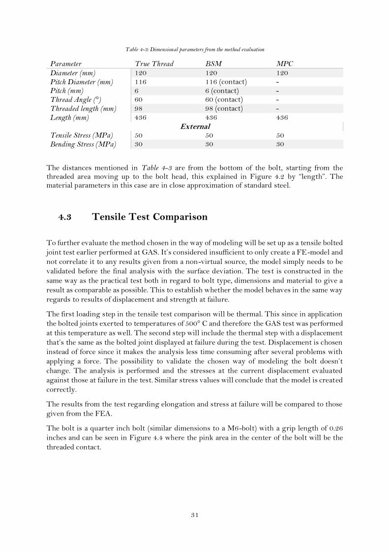
Table 4-3: Dimensional parameters from the method evaluation

Parameter True Thread BSM MPC

Diameter (mm) 120 120 120

Pitch Diameter (mm) 116 116 (contact) - Pitch (mm) 6 6 (contact) - Thread Angle (°) 60 60 (contact) -

Threaded length (mm) 98 98 (contact) -

Length (mm) 436 436 436

External Tensile Stress (MPa) 50 50 50 Bending Stress (MPa) 30 30 30

The distances mentioned in Table 4-3 are from the bottom of the bolt, starting from the threaded area moving up to the bolt head, this explained in Figure 4.2 by “length”. The material parameters in this case are in close approximation of standard steel.

4.3 Tensile Test Comparison

To further evaluate the method chosen in the way of modeling will be set up as a tensile bolted

joint test earlier performed at GAS. It’s considered insufficient to only create a FE-model and

not correlate it to any results given from a non-virtual source, the model simply needs to be

validated before the final analysis with the surface deviation. The test is constructed in the

same way as the practical test both in regard to bolt type, dimensions and material to give a

result as comparable as possible. This to establish whether the model behaves in the same way

regards to results of displacement and strength at failure.

The first loading step in the tensile test comparison will be thermal. This since in application

the bolted joints exerted to temperatures of 500° C and therefore the GAS test was performed

at this temperature as well. The second step will include the thermal step with a displacement

that’s the same as the bolted joint displayed at failure during the test. Displacement is chosen

instead of force since it makes the analysis less time consuming after several problems with

applying a force. The possibility to validate the chosen way of modeling the bolt doesn’t

change. The analysis is performed and the stresses at the current displacement evaluated

against those at failure in the test. Similar stress values will conclude that the model is created

correctly.

The results from the test regarding elongation and stress at failure will be compared to those

given from the FEA.

The bolt is a quarter inch bolt (similar dimensions to a M6-bolt) with a grip length of 0.26

inches and can be seen in Figure 4.4 where the pink area in the center of the bolt will be the

threaded contact.

32

Figure 4.4: INCO 12-point bolt model used in the tensile test comparison.

The model consists of four main parts, the bolt and nut components and a structure to be able

to implement the tensile load with contacts that occurs during application of a bolted joint.

The third component, the so-called structure is in fact two parts that can be separated. The

parts are completely similar for the exception of one being the others reflection along the axial

direction. The parts need to be able to separate since this where the force is applied by a thin

and stiff material going in between the gap of the third component and pull along the axial-

direction of the model i.e. bolt, nut and structure components. The nut is of the earlier

mentioned Waspaloy material, quarter inch in size. The same as the bolt, the 12-point nut

used in the tensile test comparison can be seen in Figure 4.5.

Figure 4.5: 12-point nut with an M6 thread in Waspaloy material.

33

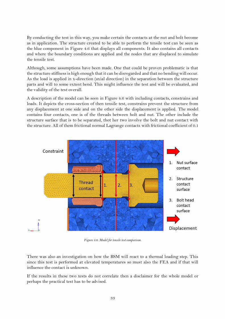
By conducting the test in this way, you make certain the contacts at the nut and bolt become

as in application. The structure created to be able to perform the tensile test can be seen as

the blue component in Figure 4.6 that displays all components. It also contains all contacts

and where the boundary conditions are applied and the nodes that are displaced to simulate

the tensile test.

Although, some assumptions have been made. One that could be proven problematic is that

the structure stiffness is high enough that it can be disregarded and that no bending will occur.

As the load is applied in x-direction (axial direction) in the separation between the structure

parts and will to some extent bend. This might influence the test and will be evaluated, and

the validity of the test overall.

A description of the model can be seen in Figure 4.6 with including contacts, constrains and

loads. It depicts the cross-section of then tensile test, constrains prevent the structure from

any displacement at one side and on the other side the displacement is applied. The model

contains four contacts, one is of the threads between bolt and nut. The other include the

structure surface that is to be separated, thot her two involve the bolt and nut contact with

the structure. All of them frictional normal Lagrange contacts with frictional coefficient of 0.1

Figure 4.6. Model for tensile test comparison.

There was also an investigation on how the BSM will react to a thermal loading step. This

since this test is performed at elevated temperatures so must also the FEA and if that will

influence the contact is unknown.

If the results in these two tests do not correlate then a disclaimer for the whole model or

perhaps the practical test has to be advised.

34

4.4 Surface deviation

After the examination of the tensile test values are provided and compared to that of the

simulations and the values bestowed there. Main focus is set to evaluate the influence of

surface deviation on strength and fatigue strength limit on the bolted flanges. This is set to

primary be done by varying the angle of deviation and see how stress concentrations and

deformations through tensile stress and bending moment and calculated its influence on

strength levels.

For this analysis, another type of bolt and nut are modelled, the new models are created as an

imaging of a hexagonal bolt and nut. Both with M6 standards. The bolt is displayed in Figure

4.7 with an explanation of the contact surfaces used in the analysis (purple) and where the pre-

tension is applied.

Figure 4.7. Depicts the M6 bolt and explains contact surfaces and pre-tension.

The bolt includes similar surfaces for contact but does not include any pre-tension elements.

The model of the bolt is depicted in Figure 4.8 with including hexagonal elements at the

contact surfaces (blue).

35

Figure 4.8. Shows the M6 bolt and displays where the contact surfaces are, including the thread contact.

This is done by modeling a circle sector of the hull and flange of the engine, the sector is

modelled in that way that it contains one bolted joint with boundary constraints to oversee

the whole component. The deviation is achieved by remodeling the solid of the flanges that

are hold together by the bolted joint, adding an either positive or negative inclination of the

surface in radial direction. The same loads and boundary conditions are applied to each model,

to later on be able to evaluate the differences between them.

The model is translated into a cylindrical coordination system to be able to apply the

symmetry in phi-direction. This since creation the whole model would be inappropriate, the

model would become too large and the number of nodes and elements the analysis would be

extremely time consuming. The model would need to have around 500 000-1000 000

elements, roughly between 1-2 million nodes and can be seen. A model including the whole

flange and all bolted joints would make those number increase with a factor of 12. Leaving the

analysis to take weeks impossible during this project.

The full model is depicted in Figure 4.9, it displays the surface constrain that gives the

symmetry in phi-direction, the applied loads and the node constrain to able to apply the loads.

36

Figure 4.9. Displays the model for investigating the influence of surface flatness.

The bolted joint components are not the same as those used in the tensile test. To get a more

general view of the influence the joint component are made in SI-units instead of imperial

measurements. The bolt and nut are M6 and both of have a hexagonal head instead of the

earlier Aerospace specific 12-point. The Joint is displayed in Figure 4.10 which is an

enlargement of the flange model in Figure 4.9. The pretension placement and normal

Lagrange contact surfaces are also explained in this picture. The contacts include

Figure 4.10: Magnification of the model in figure 19 with a 0.5-degree inclination on the flange surface.

Current model is estimated to take around a day’s work, 8-15 hours depending on the

deviation of the flange surface making the model harder to compute. This because GAS kindly

have allowed the usage of 6 CPUs for each FEA and two licenses allowing two processes to

evaluate parallel. Although, there’s a lot of trial and error regarding the FEAs to decrease the

number of errors and warnings so the second license become useful first when the model and

APDL-file correct.

37

The pre-tension is set as the first loading step to 8 kN, which is relatively low. This induces a

stress slightly higher than 30 % of the yield stress and is applied with the PSMESH. PSMESH

is a command where you specify the component and plane where the pre-tension is to be

applied. The program simply splits the elements and apply the pre-tension. To apply this in

the best manner possible the mesh is aligned, by creating a surface in the solid that the

elements will set. This will give more points where the pre-tension can be applied since the

nodes will be aligned. This is not necessary but it makes it easier to withstand complications

in the tetrahedral elements that they can be quite prone of.

The external force applied is 10 kN (4 kN in the multi-linear material model) at each surface

end of the flange in x-direction in Figure 4.9 and Figure 4.10 that will try to separate the two

flanges. To make sure the load is applied correctly there’s also a boundary condition in one

node, that won’t let that node move in x-direction. This is considered to be a better and more

uniform approach than simply lock one flange and apply the force on the other.

The test is set to evaluate the situation at 7 different cases of a deviating surface, ranging

through -2°, -1°, -0.5°, 0°, 0.5°, 1°, 2°. Negative values being when the outer part of the flange

has a gap and reversely for the positive, this depicted in Figure 4.11. All these models are set

to be evaluated linearly to begin with and if possible later on be performed as a non-linear

analysis. Considering the models sheer number of nodes, elements and contacts there might

be hard to achieve a non-linear result in both a time- and convergence perspective. Therefore,

a linear analysis is performed initially.

Figure 4.11. Displays the definition of a negative inclination (left) and a positive inclination (right).

To evaluate the pre-tension, if it’s even possible for the 8 kN pre-tension to close the gap and

if there’s a difference between a negative and positive inclination. If there is it might be an

indication of that the tolerances on the flanges should be set around another value than 0°

that is today.

Further, evaluate the contact between the flanges this might also give indications if there’s

benefit to having a negative inclination compared to a positive one, for example. To investigate

38

how the applied pre-load are able to close the gap caused by the deviating surface. Further

how the contact surface between the set contact behave,

Finally, there will be investigation of the stress concentrations around the bolt head, this to

be able to see the potential decline in fatigue life strength from a deviation. This from

investigating the stress levels, plastic strain both at pre-load and with external load applied

and compare the FSL for the models through Basquin’s law.

39

5. Results

This chapter is set to evaluate results given by performing the simulations described in

chapter 4. This will correspond to the simpler evaluations of methods to the more complicated

and elaborated evaluation of the effect of surface deviation.

5.1 Contact Method Evaluation

The analysis began with simply trying to get an understanding of how the contact method

behaves and if this could be a suitable way to perform latter analyses. Previous FEA of bolts

have been done at GAS but these where simply made and modelled with the MPC method.

Therefore, simple models were created to investigate the difference between contacts using

MPC and BSM. To establish if the BSM is suitable and if so also, how to model it for optimal

results with some help from the guidelines provided by Ansys.

Although, an examination of this shows that the contact of the thread using four elements per

pitch of the specified pitch distance become somewhat discontinuous. Instead of step-by-step

moving in the axial direction, the threads make small jump, this can be seen in Figure 5.1.

Further investigation showed that refining the mesh, now containing twice as many elements

i.e. eight in axial-direction per thread gave something a lot more similar to what an actual

thread resembles. Continuously and gradually spirally moving in the axial direction of the

bolt.

Figure 5.1. Displays the contact surface with an element size corresponding to 4 elements/pitch in the axial direction.

40

Figure 5.1 can be compared to Figure 5.2, where the contact forces can be seen for the finer

mesh that uses 8 elements per thread. The contact with the finer mesh moves more gradually

than the rougher one, displaying something that resembles a thread in a better way.

Figure 5.2. Shows the contact forces when the mesh is refined to have 8 elements per thread.

The contact area improves vastly and become more continuous looking far more like an actual

thread and promising for further analysis with the BSM.

The result from the BSM is considered more promising than that of the MPC that totally

neglects the influence of the threads and seems to overrate the bending stiffness in comparison

to the BSM. The displacement also differs to some degree but this will be investigated in

greater detail during the method evaluation in chapter 3.2 Method Evaluation.

What also was decided from the information gathered was that future analysis would be

performed with a complete model of the bolt. This since removing half of the contact surface

made it hard to decide whether the contact was implemented correctly. The uncertainty if the

thread was continuous couldn’t be had, which occurred with a half model with z-x-plane as a

symmetry plane. Although the surface in Figure 5.2 is half, it’s a complete three-dimensional

model that has been masked to display the inside (i.e. the threads in the substrate).

41

5.2 Method Evaluation

First results provided by comparing the different types of methods that can be used analyze a

bolt and bolted joints. To see for how example the contact areas will differ between the way

of modeling. To see how well the methods will take into account the formation and influence

of the threads on contacts between surfaces. The mentioned methods are Multiple Point

Constraint (MPC), Bolt Section Method (BSM) and True Thread Modeling (TTM).

Therefore, the main focus is on the Bolt Section Method provided in Ansys and the True

Thread Analysis with a purpose to comparing advantages and disadvantages for future use. It

was set to further evaluate this BSM in regards to mesh refinement, the element size needed

to get at proper analysis that will most correctly display the influence of the threads, partly

done in 5.1. Of course this is also compared to the time elapsed during the simulation since

and decrease element size will exponentially increase the time it will take to perform the

simulation [19]. Even though in most cases a finer mesh will provided better results there

has to be some regards to the computational time since there’s a time dependency on the

master thesis.

The provided information about the time difference between the different analyses are not

comparable to the FEAs performed in this thesis. This might occur due to the changes done

to the model and loading setup, but the increase seems far too high. The information describes

a difference to the MPC by a factor of 1.08 for BSM and 18 for TTM which aren’t the case

during these simulations [21]. The result and comparison in regards to time can be found in

Table 5-1.

Table 5-1: Method and time comparison

Method Number of elements Elapsed time (s) Elapsed time compared to MPC

TTM 1111133 317972 37,75941

BSM 69061 14450 1,715948

MPC 69061 8421 1

This is a more complex analysis than the earlier one set to look into mesh size and thread

creation in 5.1 Contact Method Evaluation and will help to compare with the TTM and MPC.

So, through this comparisons between the methods can be made, this is especially done to

evaluate the displacement to understand the threads influence on stiffness. This will be

interesting since future analysis will be done with a bending load, high stiffness may have a

large influence on this. These two models that are compared is a M120 bolt with a pre-tension

of 256446 N. The difference between the two models are of course the modelled threads in the

first one and a larger element size in the second one that treats the BSM. Otherwise the

materials and dimensions do not differ.

Step 1 of the analysis are set to investigate the influence of tensile stresses in bolt and

especially contacts. The loads are described in Table 4-2. The results seen and described by

Figure 5.3 show how very little differ between the TTM and the BSM but a greater difference

to the MPC. The stiffness is overestimated using this simplistic method of evaluating bolt

contacts, which was hypothesized after chapter 3.1 Contact Method Evaluation.

42

Note that the maximum value for each method in Figure 5.3 displaying the displacement when

the tensile load is applied must be handled carefully. Some elements at the peripheral top, of

the TTM bolt model where the load is applied behaves rather strange and might allow a

deflection that is too large. At the same time, the nodes closer to the center allows less

deformation.

Taking that out of consideration the behavior of TTM and BSM is very similar which is

promising for future analysis.

Figure 5.3: Displacement in axial direction (mm) of the bolt when tensile load applied (TTM, BSM and MPC respectively).

To achieve improved information of the deformation central nodes of the bolt in the z-x-plane

from Figure 5.3 along the y-axis in from bottom of the bolt to the top are analyzed in regard

to how they are displaced. The distance covered by threads are 98 mm and displayed in Figure

5.4 by a black line. The behavior of all three models are similar although, the MPC allows

lower displacement. The other two methods are so similar that most True thread line can’t be

seen since it’s at the same location as the BSM. They do separate from one another during the

last 50 mm of the central axis, this is might occur due to that the element size differs between

the BSM and TTM. This since a smaller element size will increase the number of nodes that

are analyzed which in turn will give a better assessment of the displacement, larger elements

will increase the margin of error since fewer calculations are performed [22].

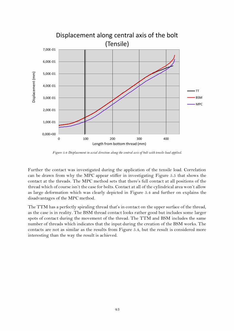
43

Figure 5.4: Displacement in axial direction along the central axis of bolt with tensile load applied.

Further the contact was investigated during the application of the tensile load. Correlation

can be drawn from why the MPC appear stiffer in investigating Figure 5.5 that shows the

contact at the threads. The MPC method sets that there’s full contact at all positions of the

thread which of course isn’t the case for bolts. Contact at all of the cylindrical area won’t allow

as large deformation which was clearly depicted in Figure 5.4 and further on explains the

disadvantages of the MPC method.

The TTM has a perfectly spiraling thread that’s in contact on the upper surface of the thread,

as the case is in reality. The BSM thread contact looks rather good but includes some larger

spots of contact during the movement of the thread. The TTM and BSM includes the same

number of threads which indicates that the input during the creation of the BSM works. The

contacts are not as similar as the results from Figure 5.4, but the result is considered more

interesting than the way the result is achieved.

0,00E+00

1,00E-01

2,00E-01

3,00E-01

4,00E-01

5,00E-01

6,00E-01

7,00E-01

0 100 200 300 400

Dis

pla

cem

ent

(mm

)

Length from bottom thread (mm)

Displacement along central axis of the bolt (Tensile)

TT

BSM

MPC

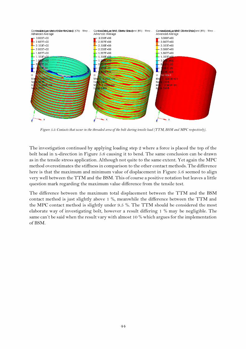
44

Figure 5.5: Contacts that occur in the threaded area of the bolt during tensile load (TTM, BSM and MPC respectively).

The investigation continued by applying loading step 2 where a force is placed the top of the

bolt head in x-direction in Figure 5.6 causing it to bend. The same conclusion can be drawn

as in the tensile stress application. Although not quite to the same extent. Yet again the MPC

method overestimates the stiffness in comparison to the other contact methods. The difference

here is that the maximum and minimum value of displacement in Figure 5.6 seemed to align

very well between the TTM and the BSM. This of course a positive notation but leaves a little

question mark regarding the maximum value difference from the tensile test.

The difference between the maximum total displacement between the TTM and the BSM

contact method is just slightly above 1 %, meanwhile the difference between the TTM and

the MPC contact method is slightly under 9.5 %. The TTM should be considered the most

elaborate way of investigating bolt, however a result differing 1 % may be negligible. The

same can’t be said when the result vary with almost 10 % which argues for the implementation

of BSM.

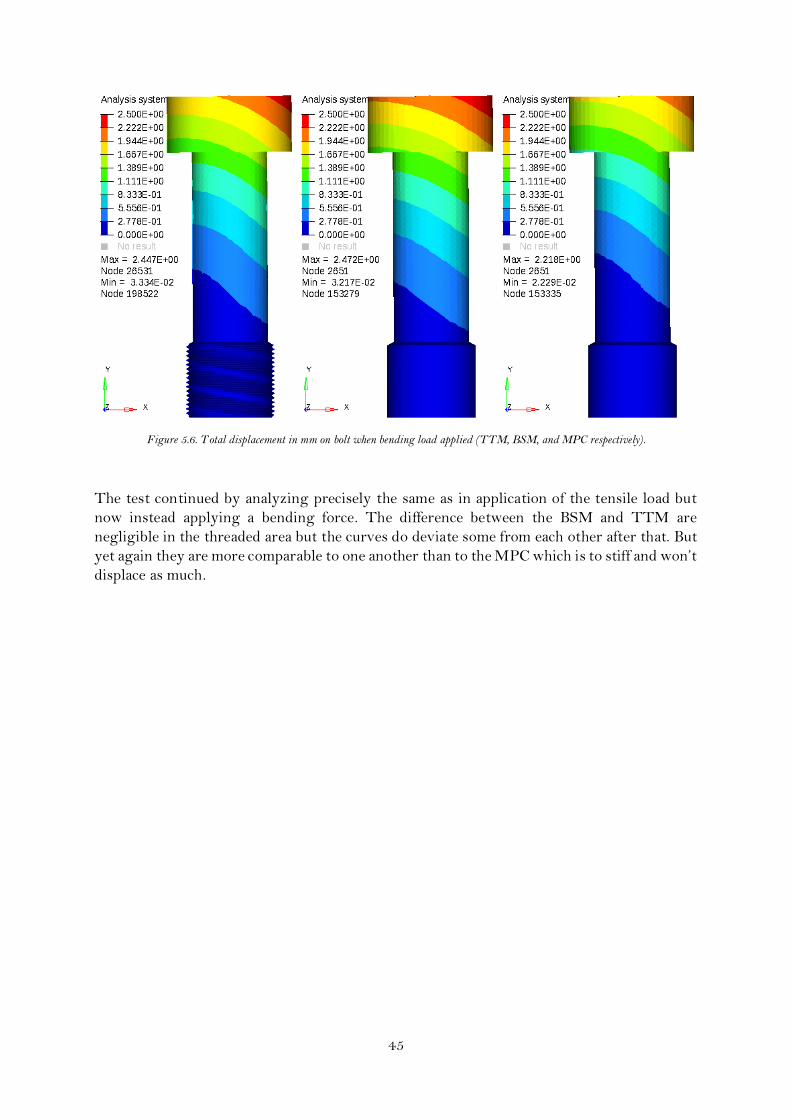
45

Figure 5.6. Total displacement in mm on bolt when bending load applied (TTM, BSM, and MPC respectively).

The test continued by analyzing precisely the same as in application of the tensile load but

now instead applying a bending force. The difference between the BSM and TTM are

negligible in the threaded area but the curves do deviate some from each other after that. But

yet again they are more comparable to one another than to the MPC which is to stiff and won’t

displace as much.

46

Figure 5.7. Displays the total displacement of the bolt nodes along the central axis of the bolt.

Looking at the surface in contact in Figure 5.8 during bending there’s absolutely no difference

for the MPC contact in comparison to the tensile loading step (Figure 5.5). As expected since

the components a meshed together.

The interesting part when looking at the contact surface during bending in Figure 5.7 is the

difference that occur between the TTM and BSM. The difference being that the true thread

seemed to be relieved from contact on the upper part in the direction where the load is applied.

No difference can be seen on the opposite side. But the BSM contact reacts in the opposite

way, instead of being relieved on one side there’s an increase of the area in contact.

0,00E+00

5,00E-01

1,00E+00

1,50E+00

2,00E+00

2,50E+00

0 50 100 150 200 250 300 350 400 450

Dis

pla

cem

ent

(mm

)

Length from bottom thread (mm)

Displacement along central axis of the bolt (Bending)

BSM

MPC

TT

47

Figure 5.8: Surface contact during bending where red displays closed and sticking, yellow closed and sliding and blue open (no contact) (TTM, BSM, and MPC respectively).

The final step of the examination of the bending loads influence is how the bending moment

will cause the surface to deviate. Both at the top part of the contact surfaces and at bolt head.

This is done by measuring the difference in axial distance between the two nodes furthest

apart in x-direction of Figure 5.6. The angle is then given by calculating arc tangent of the

axial displacement through the distance between the nodes. Since the load is exerted in the x-

direction, so is the surface deviation. The result follows in Table 5-2.

Table 5-2: Cross sectional area angularity

Method Angle at thread

Angle at bolt head

Comparison at thread (TTM)

Comparison at head (TTM)

True Thread Modeling 0.050° 5.065° 1 1 Bolt Section Method 0.048° 5.135° 0.96 1.014 Multi Point Constraint Method 0.017° 4.894° 0.34 0.9662

How the angle is evaluated are explained in Figure 5.9.

48

Figure 5.9. Explains how the angularity in table 5-2 is measured.

The most relevant from Table 5-2 is the third column of result, explaining how well the MPC

and BSM correspond to the result from the true thread modeling. This concludes with all

other results from the method evaluation that the MPC overestimates the stiffness if TTM is

considered the most thorough way to FEA bolted joints. The variation between the contacts

that takes the thread into account is 4 % and corresponds to 0.002°. This have to be considered

a small difference on a M120 bolt which has 98 mm of the bolt covered in threads.

Also interesting is column 4 that BSM later surpasses the TTM in regards to deflection even

though material properties, dimension, loads, element type and boundary conditions are all

the same. Leaving only one option for the difference, element size since it’s the only thing that

vary between the two models when the threaded area is surpassed in Figure 5.7.

49

5.3 Tensile test

To further evaluate the BSM to actual data a tensile test simulation is performed. A model is

constructed, as closely as possible resembling that of earlier performed practical test executed

at GAS. The test was conducted in an environment imitating those conditions where the

bolted joints are applied. In this case a temperature dependent orthotropic material has to be

constructed since the temperature during application is around 700 K.

The test is a very basic where the bolted joint is rigged in a structure where the components

can be separated with a tensile force applied within the grip length. The force is increased

until some component of the bolted joint gives in and complete failure occur and during this

experiment values can be extracted in the regard to yield stress and displacement at failure.

The modeled structure can be seen in Figure 4.6, where the load is applied at the ends of the

structure in one part and locked with boundary conditions at the other end.

There were a few notable and unanticipated results from the test. The first one regarding the

BSM, up to this point there could be seen that the contact is deforming the bolt as threads

would. But in this test further reasons to propagate that the BSM is a valid option for bolted

joint simulations regarding deformations.

The first interesting results were found at the contacts seen in Figure 5.10 where the two-

dimensional contact surface creates deformations that actually implies there are threads. It

can be seen by the wave-form deformation on the bolt surface, which looks like threads. This

has not been seen in any of the earlier simulations but is another positive aspect that comes

with the BSM.

Figure 5.10. Shows deformations that take form of three-dimensional threads.

The second unanticipated prospect that the BSM displayed during this test was the fact that

a rotation occurs. That applying the tensile stress causes the bolt to start threading out of the

nut. Unexpected but positive in remarks to the BSM, this since it would be expected from a

50

non-virtual practical test. All similarities in the virtual analysis that concurs with the practical

strengthens the case for utilization of the contact method. This also concurs with the choice

to create the whole model; the rotation would make a construction of the half model to save

time inconclusive. Luckily, the correct choice was made in 4.1 Contact Evaluation, otherwise

it would have rendered an incorrect analysis from the tensile test. The rotation can be seen in

Figure 5.11, where the bolt starts to thread out of the model.

Figure 5.11. Shows the von Mises stress levels of the tensile test with a magnification of a factor 100 of the occurring deformation. This

displays that the contact-modeled threads actually cause the bolt to rotate.

By rotating, this shows that to use the BSM correctly the whole bolt and nut must be

modelled. The models that was constructed to evaluate the BSM in section 5.1 Contact

Method Evaluation had a symmetry in the z-x-plane. This result of rotation shows that those

models cannot be used for a correct analysis of the problem. In section 5.1 it was concluded

that by constructing half the model would give insufficient information about the threads, this

now adds another reason that causes the model to be directly incorrect. The rotation renders

that such a symmetry would not be applicable.

Also, a problem occurs that hasn’t transpired before. During the analysis of the simulation the

BSM contact doesn’t occur at a small sector of the bolt. 1/24 part of the threaded area are not

exerted to any stresses and the problem doesn’t seem to be caused by the parameter input

about the BSM in Ansys, this seen in Figure 5.12. This was thoroughly investigated by

changing all relevant parameters to see if any other result could be achieved, but no changes

where found.

The only difference from earlier analyses using the BSM is the thermal loading step and by

applying the second step the bolt contact occurs once more. The difference from step 1

(thermal load) and step 2 (displacement) can be seen. Noted should be that in step 2 the

analysis starts at the end of the results from step 1. So, in Figure 5.12 the bolt on the right

depicts contact forces occurring due to a difference in thermal expansion between the INCO

bolt and the Waspaloy nut. The bolt on the left depicts the contact forces at the threads due

to both difference in thermal expansion and a displacement.

51

Figure 5.12. Comparison of the contact forces (N) from 1 (left) and step 2 (right) and scaled to visualize the thread contacts.

The tensile test was also set up to evaluate how well the created model corresponds to real

life by comparing the model to an earlier performed tensile test. However, the simulation was

not able to converge at the displacement that occurred during the tensile test. The multilinear

material was able to plasticize to a small degree seen in Figure 5.13, but only to 60 % of the

extent at were complete failure occurs according to the GAS experiment.

At 60 % of the displacement, the bolt and joint plasticize only in the areas most susceptible to

high concentration of stresses. This can be seen in Figure 5.13, where plastic deformation

occurs in the threads of the bolt and bolt head in particular. The plasticity that do occur are

relatively shallow and at no cross-section in the model is it completely plasticized.

Figure 5.13. Depicts the total plastic strain that occurs in the bolted joint and the threads of the bolt during the tensile test.

Investigating the bolt there’s also found that it goes through plastic deformation, mostly at

the contact surface but some can also be seen in the threads.

52

Figure 5.14. Total plastic strain that occurs in the bolt during the tensile test.

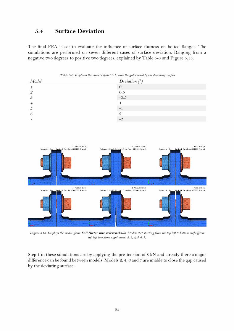
53

5.4 Surface Deviation

The final FEA is set to evaluate the influence of surface flatness on bolted flanges. The

simulations are performed on seven different cases of surface deviation. Ranging from a

negative two degrees to positive two degrees, explained by Table 5-3 and Figure 5.15.

Table 5-3. Explains the model capability to close the gap caused by the deviating surface

Figure 5.15. Displays the models from Fel! Hittar inte referenskälla. Models 2-7 starting from the top left to bottom right (from

top left to bottom right model 2, 3, 4, 5, 6, 7)

Step 1 in these simulations are by applying the pre-tension of 8 kN and already there a major

difference can be found between models. Models 2, 4, 6 and 7 are unable to close the gap caused

by the deviating surface.

Model Deviation (°)

1 0 2 0.5 3 -0.5

4 1

5 -1

6 2 7 -2

54

Table 5-4. Explanation of the model number and surface deviation

Model Deviation Able to close gap

1 0 No gap at any point.

2 0.5 No 3 -0.5 Yes 4 1 No

5 -1 Yes

6 2 No

7 -2 No

From Table 5-4 it can be seen that it’s more problematic for the pre-tension to compensate

for the gap caused by the deviating surface when the deviation is negative. Even in model 7

the gap is nearly closed, model 7 is closer than model 2 to compensate the surface deviation.

The interest in closing this gap comes from the pressure that are within the flange structure,

for the engine needs to reach a higher pressure than that of the outside surrounding. If a gap

exist it will cause leakage, leakage will in turn prohibit the engine from reaching its full

potential and the efficiency decreases. Model 7 will at one point leave an open path causing a

free flow out of the hull, highly problematic. This is done by studying the model’s

displacement after applying pretension.

This can be further seen by investigating the contact surface between the two flanges. For the

hull component that includes the flange, it’s preferred to have the contact occur at as close

approximation as possible to the web or hull. The contact surface from model 1 is displayed

in Figure 5.16.

Figure 5.16. Displays the contact status between the flanges in model 1 where 3 is closed contact and stick, 2 is closed contact that’s sliding and 1 is considered open but near contact.

This contradict the result Table 5-4 some, since evaluating the contact surface displays large

areas of blue which explains the contact to be open but close to contact in Figure 5.16 and

Figure 5.17. In the models with positive inclination the contact surface moves outwards on

55

the flange and in the negative they can be seen to decrease in bonded area (red). Model 7 is

only in bonded contact in the inner part of the flange.

Figure 5.17. Displays the contact between the flanges in model 2-7 where 3 is closed contact and stick, 2 is closed contact that’s sliding and 1 is considered open but near contact.

By removing the flange component and nut the stresses in the bolts can be examined and the

stresses in the bolt in model 1 can be seen in Figure 5.18 where only the pre-tension is applied.

This from the first evaluation of a linear material implemented.

Figure 5.18. Displays the normal stress (Pa) distribution in axial direction of the bolt on model 1 where red is at yield.

Comparing the stresses from model 1 with the ideal surface to the deviating ones gives widely

different results. When the pre-tension is applied the deviating surfaces induce high stresses

56

and instead of having the highest stress levels in the beginning of the threads it occurs in the

phasing under the bolt head.

Figure 5.19. Normal stresses (x-direction) of the bolt for model 2, 4 and 6 in the first row and 3, 5 and 7 in the second row where red and blue regions have a normal stress with an absolute value close to the yield strength.

Comparing the highest and lowest stress levels in the different models and comparing them

to flat surface model 1.

Table 5-5: Compares highest and lowest stress levels in Pascal in the models and compare them model 1 that has a non-deviating surface

Model Max stress (Pa) Min stress (Pa) Max/Model 1 max Min/Model 1 min

2 1.98E+09 – 1.26E+09 1.74 1.58

3 2.05E+09 – 1.40E+09 1.80 1.75

4 2.93E+09 – 1.81E+09 2.58 2.26

5 3.20E+09 – 2.19E+09 2.82 2.74 6 4.26E+09 – 2.99E+09 3.75 3.74 7 4.81E+09 – 3.83E+09 4.24 4.79

Table 5-5: Compares highest and lowest stress levels in Pascal in the models and compare

them model 1 that has a non-deviating surface Gives that by introducing an inclination of 0.5

degrees the stress levels increase radically with roughly 75 %. Increasing them to such extent

that plastic deformation is likely to occur without any external forces on the flanges.

In the external loading case (step 2) 10 kN is applied on both flanges in ten sub-steps to be

able to analyze the loading case. Step 1 is still there, therefore when measuring the force

through bolt and flange it should be starting at 8 kN (preload) for both bolt and flange. Each

sub-step is an increase of the external load on the flange by 2 kN and if correctly measured,

the difference between the bolt and flange force should be the same size as the step taken in

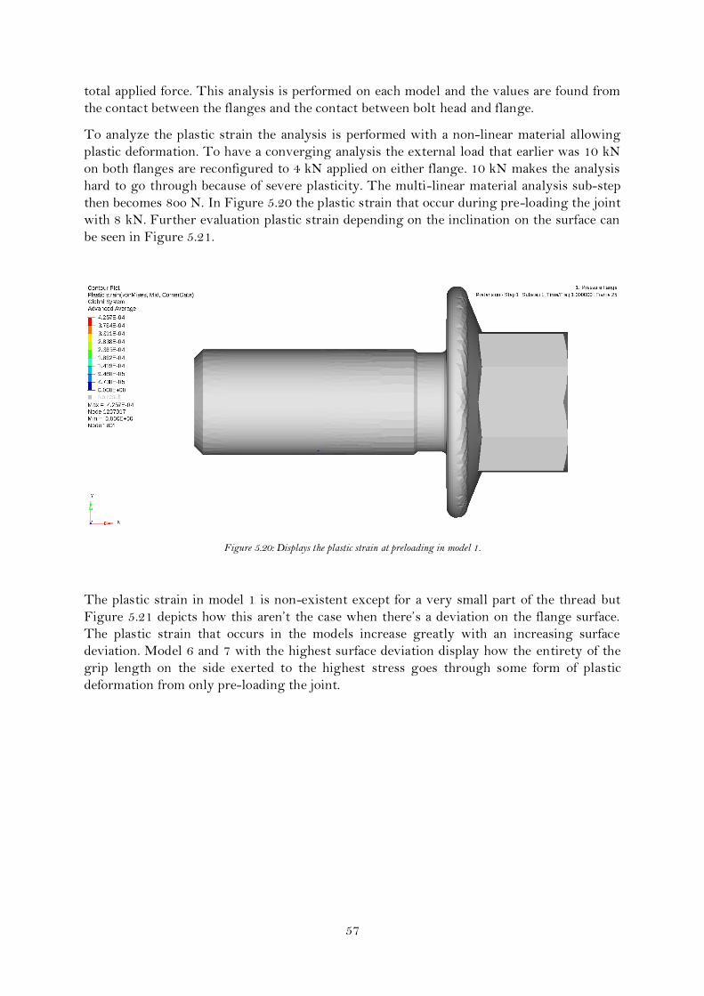
57

total applied force. This analysis is performed on each model and the values are found from

the contact between the flanges and the contact between bolt head and flange.

To analyze the plastic strain the analysis is performed with a non-linear material allowing

plastic deformation. To have a converging analysis the external load that earlier was 10 kN

on both flanges are reconfigured to 4 kN applied on either flange. 10 kN makes the analysis

hard to go through because of severe plasticity. The multi-linear material analysis sub-step

then becomes 8oo N. In Figure 5.20 the plastic strain that occur during pre-loading the joint

with 8 kN. Further evaluation plastic strain depending on the inclination on the surface can

be seen in Figure 5.21.

Figure 5.20: Displays the plastic strain at preloading in model 1.

The plastic strain in model 1 is non-existent except for a very small part of the thread but

Figure 5.21 depicts how this aren’t the case when there’s a deviation on the flange surface.

The plastic strain that occurs in the models increase greatly with an increasing surface

deviation. Model 6 and 7 with the highest surface deviation display how the entirety of the

grip length on the side exerted to the highest stress goes through some form of plastic

deformation from only pre-loading the joint.

58

Figure 5.21: Displays plastic strain at pre-load of 8 kN (from top left to bottom right model 2, 3, 4, 5, 6, 7).

Applying the full external load gives plastic strain even in model 1 with the flat flange surface

which is displayed in Figure 5.22.

Figure 5.22: Displays the plastic strain at full loading in model 1.

The already region surface that goes through plastic deformation in the deviating models are

increased even further and the severity of it as well. In model 2 and 3 with the lowest

inclination on the surface, the plastic strain is localized at the threads and bolt head. The other

models go through plasticity at other areas as well. Looking at Figure 5.23 and Figure 5.24 it

also explains that a negative surface deviation will increase the severity of the plastic

deformation in the bolt (model 3, 5 and 7). However, the section that goes through plastic

deformation in larger the positive models (2, 4, and 6).

59

Figure 5.23. Displays plastic strain at full load of 4 kN (from top left to bottom right model 2, 3, 4, 5, 6, 7).

Figure 5.24. Displays the total plastic strain straightly under the bolt head for model 2-7.

Further investigation on the von Mises stress also seem to reveal that a negative surface

inclination increases stress levels, seen through Figure 5.25 and Figure 5.26. Also Figure 5.26

reveals the thread involvement, the stresses vary and depicts a picture of the threads gradually

and spirally moving down the bolt from model 1.

60

Figure 5.25. von Mises stress at full load, red displays likelihood of plasticity in model 1.

This is even more obvious when analyzing the stresses from the deviating models. It can also

be seen that model 2, 4 and 6 have the highest stress concentration on the top surface in Figure

5.26 and the models with a negative surface inclination display the reverse, this induced by

the bending.

Figure 5.26. von Mises stress in the plastic material analysis of the bolt at full-load, red displays likelihood of plasticity (from top left to

bottom right model 2, 3, 4, 5, 6, 7).

Also interesting is the bending of the bolt during preloading the bolted joint, this is depicted

in Figure 5.27 with a magnification of the displacement by a factor of 10. The displacement

and bending are higher in the negative surface deviations, this since the flange stiffness

prohibits the closing of the gap. Bending will induce stress and the especially create a larger

stress amplitude which will lower the fatigue strength limit according to Basquin’s law and

therefore considered negative. More bending can be seen to occur with increasing surface

deviation in Figure 5.27.

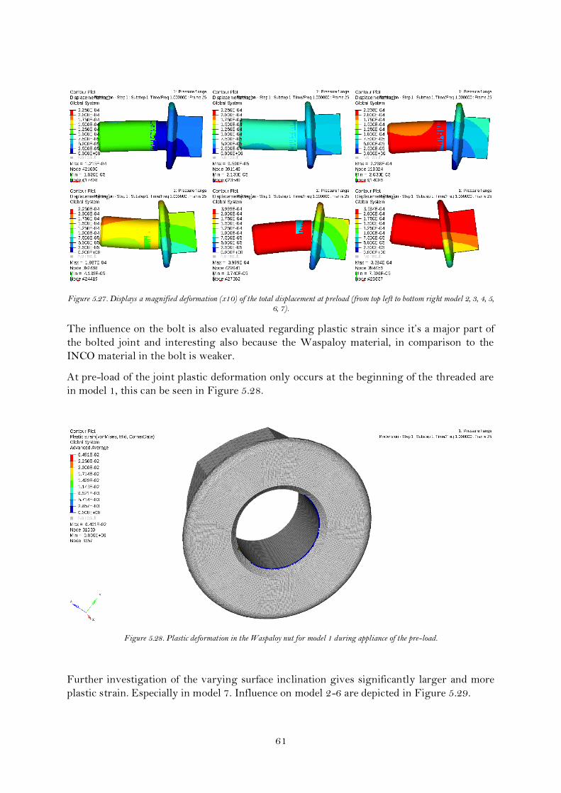
61

Figure 5.27. Displays a magnified deformation (x10) of the total displacement at preload (from top left to bottom right model 2, 3, 4, 5, 6, 7).

The influence on the bolt is also evaluated regarding plastic strain since it’s a major part of

the bolted joint and interesting also because the Waspaloy material, in comparison to the

INCO material in the bolt is weaker.

At pre-load of the joint plastic deformation only occurs at the beginning of the threaded are

in model 1, this can be seen in Figure 5.28.

Figure 5.28. Plastic deformation in the Waspaloy nut for model 1 during appliance of the pre-load.

Further investigation of the varying surface inclination gives significantly larger and more

plastic strain. Especially in model 7. Influence on model 2-6 are depicted in Figure 5.29.

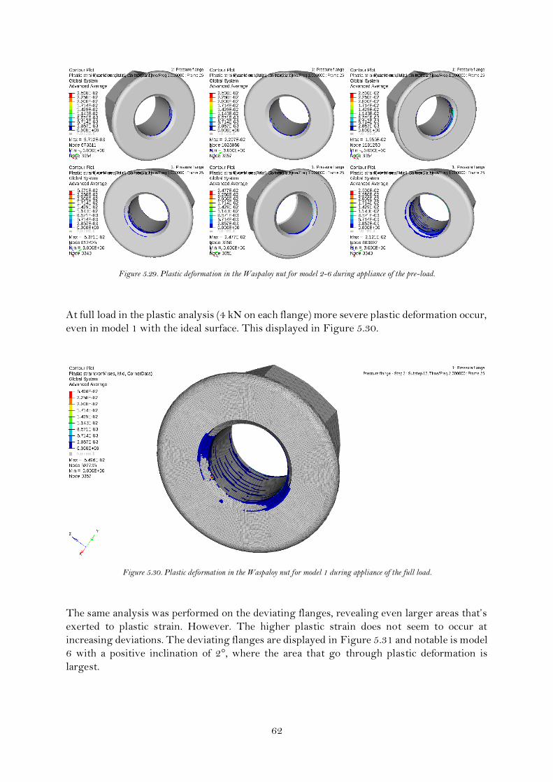
62

Figure 5.29. Plastic deformation in the Waspaloy nut for model 2-6 during appliance of the pre-load.

At full load in the plastic analysis (4 kN on each flange) more severe plastic deformation occur,

even in model 1 with the ideal surface. This displayed in Figure 5.30.

Figure 5.30. Plastic deformation in the Waspaloy nut for model 1 during appliance of the full load.

The same analysis was performed on the deviating flanges, revealing even larger areas that’s

exerted to plastic strain. However. The higher plastic strain does not seem to occur at

increasing deviations. The deviating flanges are displayed in Figure 5.31 and notable is model

6 with a positive inclination of 2°, where the area that go through plastic deformation is

largest.

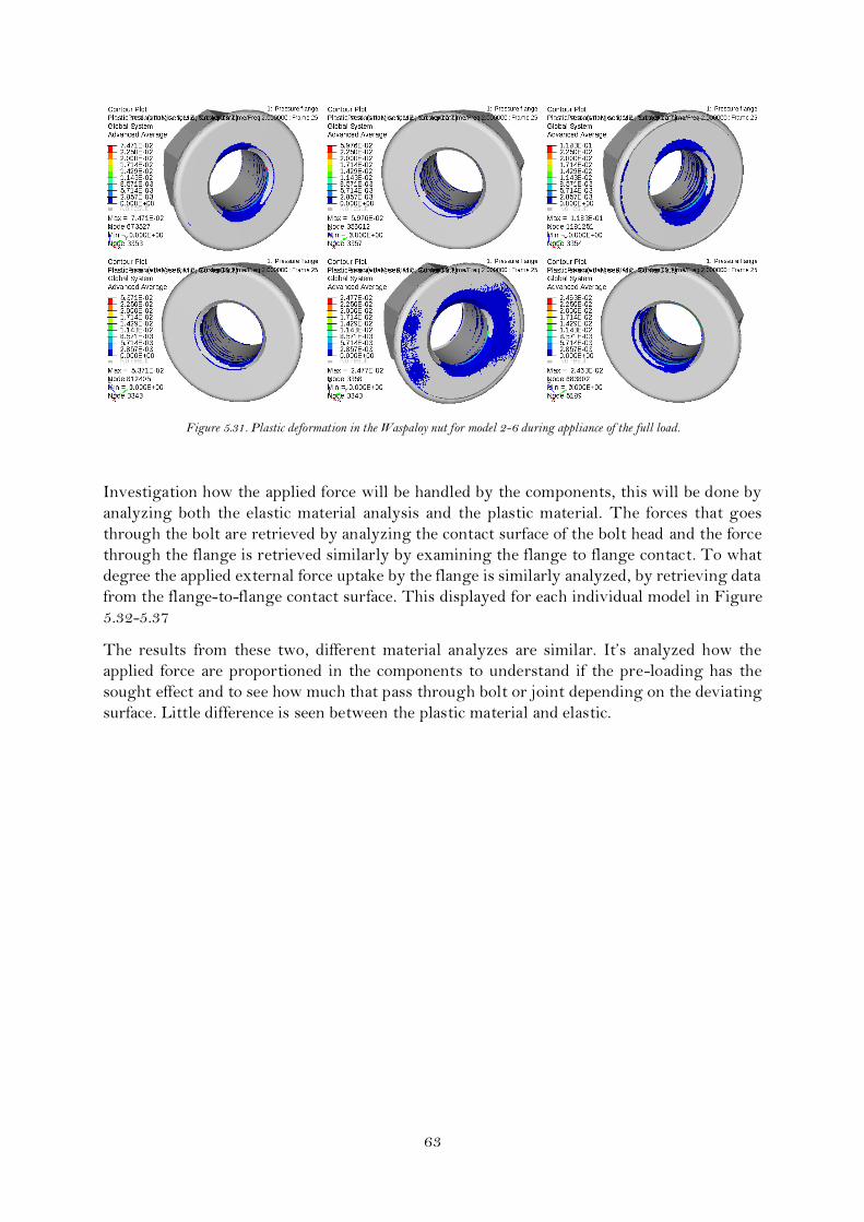
63

Figure 5.31. Plastic deformation in the Waspaloy nut for model 2-6 during appliance of the full load.

Investigation how the applied force will be handled by the components, this will be done by

analyzing both the elastic material analysis and the plastic material. The forces that goes

through the bolt are retrieved by analyzing the contact surface of the bolt head and the force

through the flange is retrieved similarly by examining the flange to flange contact. To what

degree the applied external force uptake by the flange is similarly analyzed, by retrieving data

from the flange-to-flange contact surface. This displayed for each individual model in Figure

5.32-5.37

The results from these two, different material analyzes are similar. It’s analyzed how the

applied force are proportioned in the components to understand if the pre-loading has the

sought effect and to see how much that pass through bolt or joint depending on the deviating

surface. Little difference is seen between the plastic material and elastic.

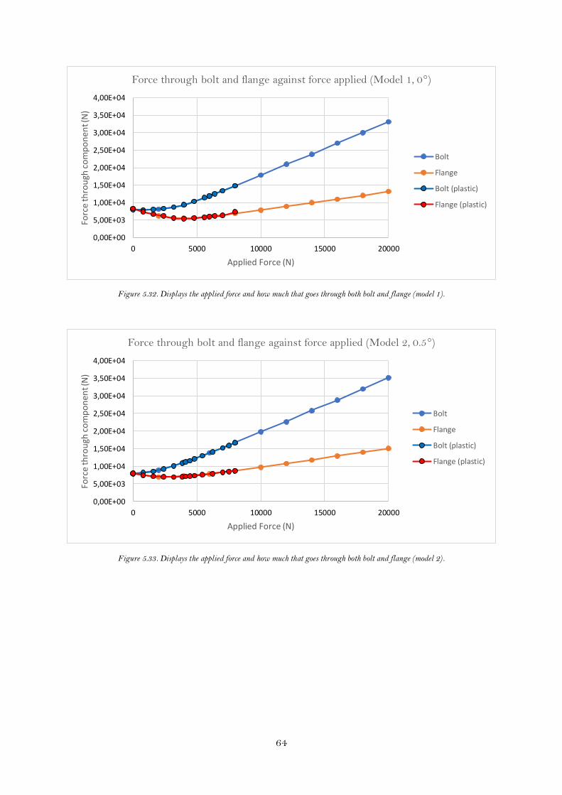
64

Figure 5.32. Displays the applied force and how much that goes through both bolt and flange (model 1).

Figure 5.33. Displays the applied force and how much that goes through both bolt and flange (model 2).

0,00E+00

5,00E+03

1,00E+04

1,50E+04

2,00E+04

2,50E+04

3,00E+04

3,50E+04

4,00E+04

0 5000 10000 15000 20000

Forc

e th

rou

gh c

om

po

nen

t (N

)

Applied Force (N)

Force through bolt and flange against force applied (Model 1, 0°)

Bolt

Flange

Bolt (plastic)

Flange (plastic)

0,00E+00

5,00E+03

1,00E+04

1,50E+04

2,00E+04

2,50E+04

3,00E+04

3,50E+04

4,00E+04

0 5000 10000 15000 20000

Forc

e th

rou

gh c

om

po

nen

t (N

)

Applied Force (N)

Force through bolt and flange against force applied (Model 2, 0.5°)

Bolt

Flange

Bolt (plastic)

Flange (plastic)

65

Figure 5.34. Displays the applied force and how much that goes through both bolt and flange (model 3).

Figure 5.35. Displays the applied force and how much that goes through both bolt and flange (model 4).

0,00E+00

5,00E+03

1,00E+04

1,50E+04

2,00E+04

2,50E+04

3,00E+04

3,50E+04

4,00E+04

0 5000 10000 15000 20000

Forc

e th

rou

gh c

om

po

nen

t (N

)

Applied Force (N)

Force through bolt and flange against force applied (Model 3, -0.5°)

Bolt

Flange

Bolt (plastic)

Flange (plastic)

0,00E+00

5,00E+03

1,00E+04

1,50E+04

2,00E+04

2,50E+04

3,00E+04

3,50E+04

4,00E+04

0 5000 10000 15000 20000

Forc

e th

rou

gh c

om

po

nen

t (N

)

Applied Force (N)

Force through bolt and flange against force applied (Model 4, 1°)

Bolt

Flange

Bolt (plastic)

Flange (plastic)

66

Figure 5.36. Displays the applied force and how much that goes through both bolt and flange (model 5).

Figure 5.37. Displays the applied force and how much that goes through both bolt and flange (model 6).

0,00E+00

5,00E+03

1,00E+04

1,50E+04

2,00E+04

2,50E+04

3,00E+04

3,50E+04

4,00E+04

0 5000 10000 15000 20000

Forc

e th

rou

gh c

om

po

nen

t (N

)

Applied Force (N)

Force through bolt and flange against force applied (Model 5, -1°)

Bolt

Flange

Bolt (plastic)

Flange (plastic)

0,00E+00

5,00E+03

1,00E+04

1,50E+04

2,00E+04

2,50E+04

3,00E+04

3,50E+04

4,00E+04

0 5000 10000 15000 20000

Forc

e th

rou

gh c

om

po

nen

t (N

)

Applied Force (N)

Force through bolt and flange against force applied (Model 6, 2°)

Bolt

Flange

Flange (plastic)

Bolt (plastic)

67

Figure 5.38. Displays the applied force and how much that goes through both bolt and flange (model 7).

Notable are the two models handling the two models with the largest surface deviation.

Figure 5.38 analyzing model 7 with the negative 2° deviation. By applying the force at the

flanges during the external loading step, at one point the two flanges are not in contact with

each other. At loading sub-step 5, where 5 kN is applied on both flanges all of the applied force

goes through the bolt and nothing through the flanges. All the force being exerted through

the bolt would be catastrophic, leading to imminent failure.

At the other side of the spectrum described in Figure 5.37 with model 6 and the positive 2°

inclination another problem occurs. The surface deviation causes the effect from the pre-

tension to be completely neglected and a bolted joint that’s not pre-loaded correctly will cause

problems. This given from gathered intel of the amplitude stresses at certain loads from the

sub-step of the applied external load. This seen in Figure 5.39.

0,00E+00

5,00E+03

1,00E+04

1,50E+04

2,00E+04

2,50E+04

3,00E+04

3,50E+04

4,00E+04

0 5000 10000 15000 20000

Forc

e th

rou

gh c

om

po

nen

t (N

)

Applied Force (N)

Force through bolt and flange against force applied (Model 7, -2°)

Bolt

Flange

Bolt (plastic)

Flange (plastic)

68

Figure 5.39. Displays external load applied to flange versus life length for the different models.

2000

3000

4000

5000

6000

7000

8000

9000

1,000E+03 1,000E+04 1,000E+05 1,000E+06

Exte

rnal

Lo

ad (

N)

Life length (Nf)

Life depending on surface deviation (r=0.1)

0.5 Degrees 0 Degrees

1 Degree 2 Degrees

-0.5 Degrees -1 Degree

-2 Degrees

69

6. Discussion

This chapter is set out to investigate the results given in the project, to decipher and interpret

the implication of the results. This will be done separately, each analyze performed have its

own sub-chapter for discussion with names corresponding to the chapter in Results.

6.1 Analysis of the Bolt Section Method

The evaluation of the bolt section method became a larger part of the master thesis than was

anticipated at the start. The method was considered a real opportunity to implement a better

way of performing FEA analysis’s on large models containing several bolts without increasing

computational time to an unacceptable level. The implementation of contact method in the

software isn’t any more complicated than the construction of any other contact. The extra

work only includes some bolt parameters and a definition of the axis and the dimensional

parameters of a colt could easily be created in a macro since its likely several bolts that have

the same dimensions. So, if a macro is created for each bolt type, there’s basically only the axis

(location of bolt) that needs to be specified. So there’s no practical reasons not to implement it

in the analysis. The contact method does need a relatively fine mesh, which may make it

unsuitable for full scale models that usually are performed in the beginning of a new project,

at GAS this example could be an engine. However, after this incipient analysis to locate

problematic areas there are sub-analyzes performed to be able to investigate more thoroughly

regarding loads and mesh. This is where the BSM could be applied to give further credence

to the analysis. Because as seen from the results and especially in 5.1 Contact Method

Evaluation and 5.2 Method Evaluation the BSM gives a more realistic behavior in regards to

thread contact. Yes, it will also increase the computational time, but this project considers a

factor of 1.7 affordable, especially when the material in the Method Evaluation involved

plasticity. Usually most analysis on larger components are first and foremost evaluated

linearly.

The first analysis in 5.1 Contact Method Evaluation does not take the whole bolt into

consideration that will be a latter improvement of the analysis. This is mainly performed for

the sake of the contact threads. Advantages and disadvantages from the evaluation can be

found in Table 6-1.

Table 6-1: Advantages and disadvantages from the three tested models in evaluation of the BSM.

Models Advantage Disadvantage Further Evaluation

x-z-symmetry, 4 elements/pitch

Fewer elements Poor thread contact.

No

Full model, 4 elements/pitch

Improved contact surface

More elements No

Full model, 8 elements/pitch

Greatly improved contact surface

Even more elements

Yes

70

Then the BSM analysis progressed through 5.2 Method Evaluation. There’s of course not as

a clear-cut contact in the BSM as in the TTM, but there’s nothing showing that the BSM

surface contact wouldn’t improve with a finer mesh. The TTM needs a very fine mesh, a

similar mesh on the BSM would most likely improve the contact surface to a more continues

and good-looking thread. But this is of point, the reason of the BSM being a viable and good

option is that there’s no need for the hyperfine mesh but still achieve impact resembling that

of threads. In the large-scale models that are evaluated at GAS there’s no interest in a perfect

contact of the threads but the influence it might have on stiffness and dislocation in stress

analysis’s is highly relevant.

In this thesis, there’s found that the bolt section method very closely resembles the true thread

modeling in both displacement and stiffness. This through the comparison mad between the

three different models in 5.2 Method Evaluation of the thesis. The difference at the contact or

thread are absolutely negligible to each other which can’t be said about the MPC method that’s

currently used during simulation of large scale models. With this showed the thesis concedes

that there’s a good reason why to implement the BSM.

However, the BSM did show some limitations during the FEAs as well. During the analysis

regarding 5.3 Tensile test the initial loading step which was thermal revealed some concerns.

The application of the thermal load lead to the contact method to completely neglect the

contact at a small part. This was the exact same size as the modeled solid from Hypermesh.

The solid was modeled as 1/24 of the total bolt and then reflected and rotated to achieve the

full bolt model. The contact goes missing at the origin of that solid, why is unclear since

there’s no problem with this in the last evaluation of surface deviation even though the models

are constructed in the same way. The only thing that tells the two analyzes apart is the

thermal loading step in the tensile test comparison and therefore precautions have to be made

when utilizing the BSM with varying temperatures.

A simple way to get around this problem is by directly use the material properties at the

certain temperature and not have a multilinear material model that adapts to temperature

change. But since the Waspaloy nut and INCO bolt does have differences in thermal expansion

the project sought to find the effects of this as well and not neglected the stresses induced by

using the bolted joint in elevated temperature applications.

Rather unexpected the 5.3 Tensile test comparison provided furthermore explanation to how

the BSM behaves, fortunately in two ways that strengthens the argument for it to be applied.

In a magnification of the problem of an early analysis with only elastic material properties it

can clearly be seen that the bolt starts to thread out of the nut, causing the bolt to rotate which

no external load would imply it should. This is viewed as a good property since this is what

would be expected in the practical test and the TTM that are seen as what the BSM should

strive to become. What this also implies is that the first analysis from the investigation on the

BSM where a symmetry in the z-x-plane was implemented is not a viable way to analyze with

the BSM. Luckily for this project the symmetry was considered bad in the way that it made

the whole contact area made it hard to analyze the formulation. But after the tensile test it can

be seen that modeling this way is completely incorrect since that symmetry does not apply

when rotation occurs.

Another notable result coming from the tensile test comparison was the deformation

occurring on the bolt surface, when magnified, the picture depicts how models actually are

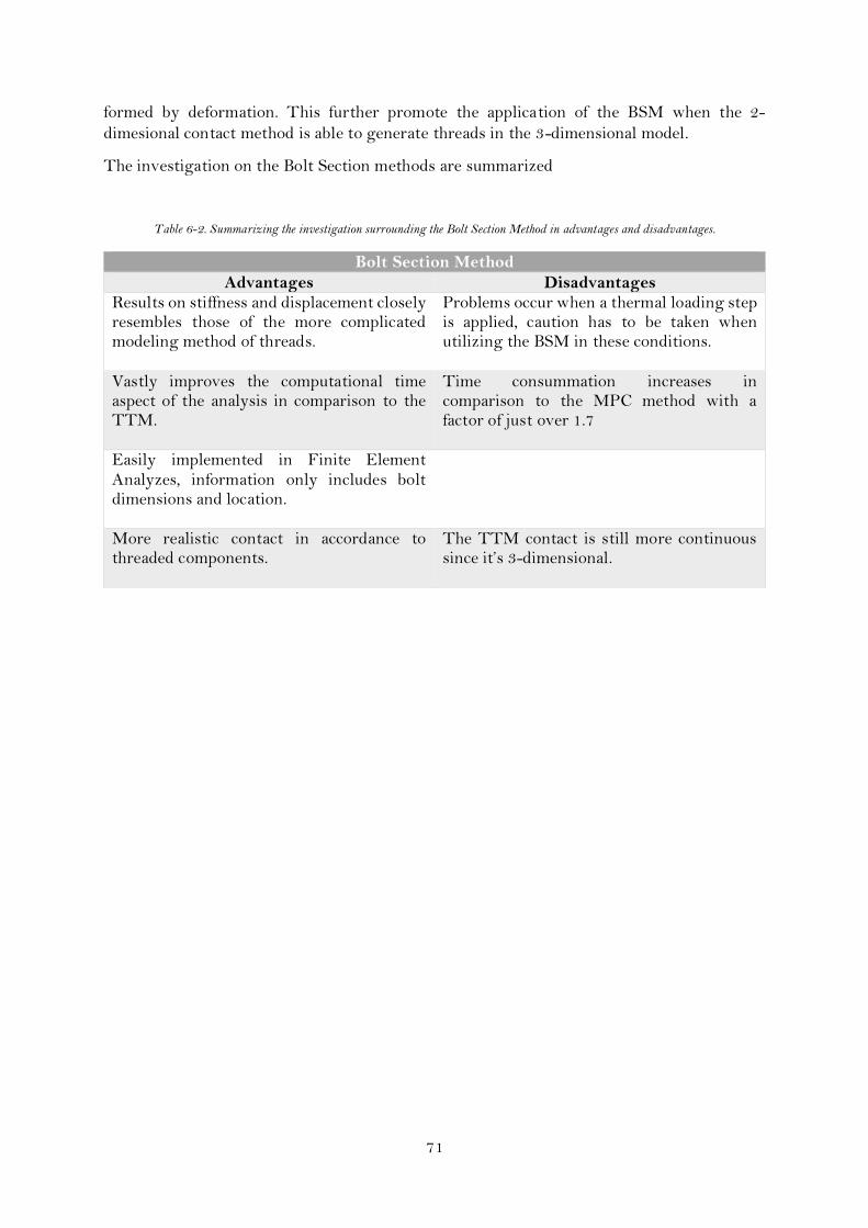
71

formed by deformation. This further promote the application of the BSM when the 2-

dimesional contact method is able to generate threads in the 3-dimensional model.

The investigation on the Bolt Section methods are summarized

Table 6-2. Summarizing the investigation surrounding the Bolt Section Method in advantages and disadvantages.

Bolt Section Method

Advantages Disadvantages Results on stiffness and displacement closely resembles those of the more complicated modeling method of threads.

Problems occur when a thermal loading step is applied, caution has to be taken when utilizing the BSM in these conditions.

Vastly improves the computational time aspect of the analysis in comparison to the TTM.

Time consummation increases in comparison to the MPC method with a factor of just over 1.7

Easily implemented in Finite Element Analyzes, information only includes bolt dimensions and location.

More realistic contact in accordance to threaded components.

The TTM contact is still more continuous since it’s 3-dimensional.

72

6.2 Method Evaluation

The fact that the analysis for the TTM analysis takes roughly 88 hours makes it unsuitable

for future FEAs. Since the future planned surface deviation investigation is set to evaluate a

number of different cases with models that most likely includes more elements and nodes.

This model of the M120 is large, but in latter FEAs there are more components, with two

flanges and a nut to be included as well. The fact that the model of the bolt will be smaller

doesn’t imply that the elements can be any larger in comparison to the model. A small model

would need smaller elements for a correct and good analysis, it’s relative to the model.

The results from the BSM are less convincing than the information provided but if considered

viable in other aspects a 71 % longer examination is acceptable. This analysis is performed in

just above 4 hours which absolutely would be acceptable in latter stages in the thesis. So even

though the results are worse than expected they are considered fully viable. From the Method

evaluation and the analysis of the BSM in the earlier sub-chapter it’s considered the best way

to analyze future problems regarding the tensile test comparison and surface deviation.

The MPC was as expected the fastest way of performing the test. But the results of the MPC

method was also worst in comparison to the TTM which was considered the most thorough

way to analyze bolted joints. The complete negligence of threads rendered it to be considered

harmful to this project.

The comparison to the information given in regard to computational time can’t be established

fully since there’s no information about how many CPUs that are used. But the factor between

them shouldn’t really be changed. With an increasing number of CPUs, the elapsed time will

decrease linearly, so twice the number of CPUs would leave the FEA to be halved. But the

results aren’t comparable in that way either, leaving a question in regards of the sources

explanation of elapsed time during analysis.

The TTM is performed as expected the computational time increase significantly since a large

number of elements is a must because of the small thread that is modelled. The specific

simulations take just short of 90 hours to perform, luckily the simulations can be left overnight

leaving it to take just 3 work-days to perform. Otherwise it would take just short of nine days

of work. The result of the simulation is great and if it wasn’t for the time parameter it would

have been most interesting to perform all simulations and analyzing this way.

But since the most important part for comparison is the threaded this result is very promising

(0-98 on x-axis). The following parts differences may occur due to the differing element size

in the models, to compensate for the extremely small elements at the thread of the TTM

simulation the element moving up to the bolt head are constructed larger than in the BSM

model. That might allow a difference.

73

6.3 Tensile Test Comparison

The tensile test comparison is left somewhat inconclusive since the model couldn’t converge

at complete plasticity of the bolt. The model is considered to be meshed to a very fine size,

however to complete the analysis it probably needs to be even more extensive in that regard.

The current analysis was performed in roughly 10 hours and considering a finer mesh would

extend this further it could not be performed. To what extent the mesh needed to be

configured to achieve this is unknown but when the model only could converge at 60 % of the

displacement of the performed test, it would probably be to a great degree. So, the results from

this analysis couldn’t give the model the credence that was sought, however two unexpected

perks from the BSM was found instead as well as a disadvantage.

To try to achieve convergence both a rigid element and a RBE3 where tested but neither of

these was a solution, instead the analysis was even further from convergence. GAS insisted it

would be performed in the same way practical test. This to conclude whether the test itself

was performed correctly.

The test is concluded to not be optimal since there’s a bending that’s not accounted for. By

applying the load in the gap between the structure and the bolt is aligned along the central

axis of the structure, the center can be reached. This will cause the structure to bend slightly

inwards, toward the central axis.

74

6.4 Surface Deviation

First and foremost, in the investigation regarding the influence on surface flatness on flanges

the ability to close the gap caused by the deviation was observed. This is relevant since there’s

lower and at some sections higher pressure inside the engine than in the surrounding

environment and that is needed for the engine to function properly. A gap between the two

underlying surfaces of the flange would increase leakage which in turn would decrease

efficiency of the engine or in fact cause it to fail.

Noted from the result is that it seems a negative inclination have an easier time closing the

created gap, this according to Table 5-3. This is explained by that the positive inclination have

clamp down the whole web while the negative only need to take the flange thickness into

regard. Looking from this perspective a negative deviation surface is better than a positive

one, the leakage would likely become lower.

Although, contradicting the previous section some, at full load model 7 would definitely have

the highest leakage. This since at one point during application of the external load of the

flange the two surfaces would completely separate. Leaving an open passage for the fluid to

travel through and severe leakage would occur.

The ability to close the gap also correlate with the next analysis regarding the contact between

the two flanges. The depictions of the contact surfaces is also after applying the pre-tension.

It’s beneficial for the construction ta have the contact center as close as possible to the web,

this will further help to prevent leakage. That can be seen though, is that the contact moves

further out on the flange on the positively deviating model (model 2, 4, 6). This also explains

that a negative inclination might be preferable in comparison to a positive one with the same

value. However, yet again model 7 contradicts this, where no influence of the preload of the

bolt can be seen at all. Leaving only a small line on the inner part of the flanges to be in

contact. Portraying model 7 as the most problematic model.

It should be noted that the results from the contact surface evaluation is with a perfect surface

roughness and the sectors that display “no-contact” doesn’t have to leak. The correlation

between the contact surface and leakage can’t be drawn conclusively. A surface roughness

would increase contact and decrease leakage.

The investigation then moved on to the linearly elastic material stress analysis after applying

the preload. The difference in stress concentration between the models are significant,

especially the highest notated stress. Even the models with the least deviating surfaces (model

2 and 3) display major rises in stress levels, in comparison to model 1 these increase by at least

70 %. Since the same pre-load are applied to all the models this tells a story of an increasing

stress intensity factor depending on the surface inclination. Higher stress concentrations will

in turn lower the components fatigue strength limit, so this is a first indication on how a

deviating surface will influence fatigue strength limit.

As mentioned, the first FEA was performed with a linear elastic material, causing the result

to display extreme values in regard to stress. Model 7 display stresses above 4 GPa, which is

well above the INCO-materials yield stress and concluded that a analysis with a multilinear

material info would provide very interesting information.

75

However, the earlier applied external load on the flanges was too high for the analysis to

converge so it was decreased with 60 % to 4 kN on each flange.

After pre-loading the ideal barely any plastic deformation has occurred, but as expected from

the linear material analysis the other models all displays signs of deformation. Increasing

severely with increasing or decreasing inclination.

The plastic strain that occurs in the bolt is increased when there’s a deviating plane, in the

models with the highest and lowest inclination on the surface (model 6 and 7 respectively)

there are very large areas that goes through plastic deformation. This occurs even when the

bolt is only exerted to the pre-load, so by simply clamping the flanges there’s severe plastic

deformation. At full loading the models doesn’t differ too much from the plastic strain that

occur during appliance of the preload, this probably comes through that in the plastic model

the pre-load and external load is of the same size. Inducing this kind of plastic strain by simply

pre-loading the bolt is worrying and to say that an inclination on the surface is bad for the

joint in the case of plastic strain would be an understatement.

What should be noted on the plastic strain analysis of the bolts in the different models are the

plastic deformation that occurs on the upper areas of the bolt head. These are most likely

exaggerated due to the models lack of phasing at the part where the structure of the bolt head

begins. This causes an unanticipated stress concentration, which when modeling was

neglected. The sharp edges will cause severe stress concentrations which in turn might give

quite a misleading description of the plastic deformation.

There is also an explanation on how the deformation looks like, the deviating models are

displayed and increasing deviation logically causes the bolts to bend more. What also can be

seen in the figure is that there seems to occur a larger deformation in form of bending on

model 3, 5 and 7 with the negative inclination.

The plastic deformation that occurred on the nut was also investigated since it’s a major part

in a bolted joint. The analysis of the plastic deformation in the nut is done in exactly the same

way as with the bolt.

Firstly, the plastic strain that occurs at pre-loading the bolted joint is studied and this depicts

that there’s very little plastic deformation at the ideal surface flatness in model 1, only the

topmost thread goes through a small deformation. Looking at the deviating models (2-6) it

can be seen here as well how the increasing or decreasing inclination also induces more areas

going through plastic deformation. Precisely the same pattern that occurs when deciphering

the results of the bolt.

However, there is a difference that occurs when looking at when the full external load is

applied. With the bolts, there wasn’t too much difference between the results from applying

the pre-load and later applying the full external load. This is not the case for the plastic strain

analysis of the nut, here it’s a clear difference. The area that goes through plastic deformation

in the nut is considerably larger when the external load is applied. This might come through

that the Waspaloy material properties are around 25 % weaker in regard to strength in

comparison to the INCO-material that are used in bolt and flange. Opposite to earlier results

as well, the more severe deformation seems to occur in the models with a positive deviation

(model 2, 4, 6). Model 2, 4 and 6 have a larger area of the contact surface going through plastic

deformation, however model 3, 5 and seven seem to have an increased number of threads that

are exerted to plastic deformation.

76

Further the result surrounding the surface deviation analysis looks at how the applied external

load is distributed in the bolted flange. This to see how well the pre-tension can be utilized in

the models. This since a properly pre-loaded bolted joint is mandatory to achieve a good

fatigue strength limit for the joint.

The models exhibiting an acceptable or good behavior in regards to this from the model 2-7

are model 2, 3 and 5. In these it can be seen how the pre-tension takes care of the external

load (until a certain point). If the load in the bolt doesn’t increase then neither does the stress

and no stress variations will prevent a stress amplitude which will decrease the fatigue

strength limit of the bolt.

By the definition above, model 7 should also be included, however the data from model 7 shows

that at one point the load through the flange is non-existent. Since the data is retrieved by

analyzing the contact between the flanges, this implies that they no longer are in contact.

Causing all the force to go through the bolt which most likely would lead to failure. Not due

to fatigue but from simply overloading the bolted joint but if the bolt would be able to handle

the load, failure due to fatigue would occur imminent. But yet again the results seem to apply

in comparison to each other, the negative inclination is the lesser of two evils and slightly

better for the construction.

Finally, the fatigue strength is evaluated and the results display what the earlier results

implies at least in comparison to model 1 with ideal surface conditions. However, there are

some anomalies, for example model 2 with the 0.5° positive inclination appear to be the worse

in comparison to model 4 which is very unintuitive. This might come through that the stress

amplitude that is utilized in Basquin’s law was hard to extract from the models. Since the

highest stress amplitude might not occur where the highest stress levels are reached. So there

are some error margins surrounding the localization of the node with the highest stress

amplitude. Otherwise the results seem to match earlier extracted information, the negative

inclination seem better than the positive one (except for model 7, again).

A deviating surface will decrease fatigue strength.

77

7. Conclusion

This chapter is set to discuss and draw conclusions from the given results during the thesis

with the major goal to evaluate the Bolt Section method in bolted joint FEAs and the influence

of surface flatness on fatigue strength limit in regard to tolerances.

7.1 BSM

The BSM is considered a viable option in this report, it’s considered a good optimization of

mechanical similarities to TTM and computational time. It’s simply implemented and using

APDL-files macros can be generated for each type of bolt and a line of code is sufficient to

implement the contact method.

7.2 Surface influence on fatigue strength limit

It can be seen that even relatively small degrees of inclination on the flange surfaces induce

significantly higher stresses in the bolt. Higher stress concentrations within a component will

directly reduce the number of cycles before failure. It can be seen by just applying the pre-

tension on the deviating surfaces induces stresses above the yield stress of bolt.

So a surface deviation do have an influence on FSL and a large one when a totally plausible

inclination on the surface will induce a roughly 70 % higher stress.

7.3 Tolerances

As seen from the results, it’s slightly better to have a negative inclination than a positive one.

The project then conclude that current tolerances that are set by the ideal surface that’s

completely flat surface should be re-advised. Tolerances should allow a slightly lower

inclination in positive direction since the positive, with a gap at the web does have a more

severe effect on leakage, contact and FSL.

78

8. Future Work

This chapter is set to discuss what the report finds relevant to further investigate and the

results given and the analysis of it.

8.1 Bolt Section Method

Further investigation surrounding the BSM has to be performed to assure its viability in

bolted joint FEAs. What’s found in chapter 3.3 Tensile Test is that the thermal loading step

seem to cause problems for the contact method. By applying the thermal load, it causes the

contact surface to completely disregard a small part of the threads leaving a 1/24 of the bolt

free from any of contact. This will cause a slight, deceptive increase in stress and force exerted

in the other nodes remaining threads.

Even stranger during the simulations to compare the model to a practically performed tensile

test is that when the displacement is exerted the contact is working again. The only conclusion

that can be drawn from this report is that the BSM is problematic to use in cases where

thermal loading occurs, or at least where there’s only a temperature increase or decrease.

This project sought to find out if there was a viable option to the true thread modeling which

is way too complicated and time consuming for implementation in large scale simulation. An

interesting point of view could be to see how rough mesh there can be and still see the

improvement compared to the MPC models. This report evaluated the recommended 4

elements/pitch and later on refined the mash to come to the conclusion that the contact

appeared more realistic then. But it may be relevant to go the other way as well, will the

mechanical properties differ with 2 elements/pitch? There’s always that consideration

between accuracy and time in FEAs, so even though the contact may appear worse it may be

a better option in a certain analysis.

It’s interesting and worrying how reluctant Ansys is to release any data surrounding how the

contact method is implemented. During this thesis, at several occasions contact was

established with both support and Ansys sales providers and neither of these could prevail the

project with any extensive explanation of the method. If this was because of lack of knowledge

or reluctance is unclear.

What is known is that there are a highly competitive market surrounding the CAE-programs

able to perform complicated FEAs and that may cause the company’s to be careful with

information and ideas.

79

8.2 Method Evaluation

The method analysis was done to depict how properties differ from each other in the three

possible ways of modeling the problem. The comparison looks at the contact surface in the

threaded area of the bolted joint components, stiffness and displacement. Further comparisons

would improve the knowledge of when in what case a method should be implemented. Even

though the lack threads in the MPC method it might be the most suitable under certain

conditions, the same in regard to the other two modeling forms. So to establish this all

parameters will need investigation, thermal conditions, electrical influence and rotation by

torque are examples. So that an engineer can look at a problem and implement the right type

of model.

8.3 Tensile Test Comparison

The tensile test comparison exhibit one property that may cause reason to reconfigure the

test if performed again in the future and that’s the bending of the structure. During GAS

practical test, the deformation at failure occurred slightly before the expected elongation and

it was never concluded why this was. The project has hypothesized that this may due to this

and recommends an evaluation of this if plans are to be performed again.

8.4 Surface Deviation

There are several important factors that surround bolted joints that’s still needs to be

investigated after this analysis, to see how they influence the fatigue strength limit when

there’s a surface deviation.

The most interesting to look at might be the pre-tension, to also be able to get knowledge

how a varying pre-tension might influence the fatigue strength. Generally, a higher pre-load

will improve mechanical abilities of the bolted joint. Looking at the M6 bolt used in this

analysis, by applying a pre-load of 8 kN the pre-tension reaches to around 30 % of the yield

strength. This may be considered quite low and therefore it would be interesting to perform

further analyses with alternative pre-tension and in particular a higher one. However, the

surface deviation results provided conclude that that pretty severe plasticity occur when

preloading with 8 kN that was investigated in this report, especially on the models with the

highest deviation (model 6 and 7). So, to establish a correlation there and further be able to

conclude at what level of deviation the constructed part become completely impracticable and

correlate tolerances according to this value. So to perform analysis on each of the models

studied in this thesis, with a range of pre-loading.

Further investigation should involve the analysis of surfaces that deviate less than the models

tested in this project. Analyzing models that increase in deviation step-by-step in the range of

0.05-0.01 to be able to achieve a more thorough and clear visualization how the fatigue

strength limit is influenced. This project is able to provide the information that a surface

80

deviation has a negative influence on the FSL, however it would be interesting to also get an

understanding to what extent.

This report analyzed the influence of a surface deviation on the bottom surfaces of the flange,

other possible outcomes should also be investigated. An inclination on the top surface of the

flange, on the bolt head or the nut are likely to have negative effects as well.

81

References

[1] Gkn.com. 2017. GKN | Engineering That Moves The World | GKN Group. [online]

Available at: http://www.gkn.com/ [Accessed 26 Apr. 2017].

[2] Boltscience.com. 2017. The Effect on the Fatigue Life of Bolts of Joint Face Angularity.

[online] Available at: http://www.boltscience.com/pages/nutfaceangularity.htm [Accessed

26 Apr. 2017].

[3] Zerofast.com. 2017. 12 POINT BOLT | zero products inc.. [online] Available at:

http://www.zerofast.com/product/12-point-bolt [Accessed 2 May 2017].

[4] Civil Engineers Forum. 2017. 5 Differences Between Bolt and Screw. [online] Available at:

http://civilengineersforum.com/bolt-vs-screw-difference/ [Accessed 26 Apr. 2017].

[5] Rolled Alloys, I. 2017. WASPALOY® - Rolled Alloys, Inc.. [online] Rolledalloys.com.

Available at: https://www.rolledalloys.com/alloys/cobalt-alloys/Waspaloy/en/ [Accessed

26 Apr. 2017].

[6] Corda, S. 2017. Introduction to aerospace engineering. 1st ed. Chichester, West Sussex,

United Kingdom: John Wiley & Sons, Inc.

[7] Lisi-aerospace.com. 2017. Self aligning Nut. [online] Available at: http://www.lisi-

aerospace.com/products/fasteners/internally-threaded/self-aligning-

nut/Pages/default.aspx [Accessed 26 Apr. 2017].

[8] Oberg, E., Jones, F., Horton, H., Ryffel, H. and McCauley, C. 2016. Machinery's handbook.

1st ed. New York: Industrial Press.

[9] Hale, S. 2015. Why Worry About Hourglassing in Explicit Dynamics? Part II | CAE

Associates. [online] Caeai.com. Available at: https://caeai.com/blog/why-worry-about-

hourglassing-explicit-dynamics-part-ii [Accessed 3 May 2017].

[10] S.K. Bhaumik, M. Sujata, M.A. Venkataswamy, Failure Analysis & Accident

Investigation Group, 2010, Microstructural study: an aid to determination of failure mechanism in

nickel base superalloy blades, Materials Science Division, National Aerospace Laboratories,

Bangalore 560 017, India]

[11] VDI 2230 Part 1 Systematic calculation of high duty bolted joints, 2003, Distribuerad

av SIS Förlag AB på licens av DIN

[12] ANSYS, Inc. 2016, ANSYS Mechanical APDL Contact Technology. 17.0 ed.

Southpointe: Ansys, Inc.

[13] Lauth, M. 2014. Workshop Bolt thread and pre-tension, , EDR MEDESO.

[14] Newsteelconstruction.com. (2017). AD 286: Preloaded Bolts: The Net Effect of Applied

Tension and Preload. [online] Available at: http://www.newsteelconstruction.com/wp/ad-

286-preloaded-bolts-the-net-effect-of-applied-tension-and-preload/ [Accessed 4 May 2017].

[15] Agatonovic.de. (2017). Auswahl - Bolt connections, Fracture mechanics, creep, Fatigue.

[online] Available at: http://www.agatonovic.de/schlane.htm [Accessed 4 May 2017].

82

[16] Brown, K.H., Morrow, C. Durbin, S, Baca. A. (2008). Guideline for bolted joint design

analysis. Alburquerque. Sandia National Laboratories.

[17] Colly Company AB, Handbok Om Skruvforband. 1st ed. Kista: Division

maskinelement, Colly Co., 1995. Print.

[18] ANSYS, Inc. 2010, ANSYS Mechanical APDL Contact Technology. 13.0 ed.

Southpointe: Ansys, Inc.

[19] Liu, G. and Quek, S. (2003). The Finite Element Method. 1st ed. Oxford: Butterworth

Heinemann, p.247.

[20] ANSYS, Inc. 2016, ANSYS Mechanical APDL Element References. 17.0 ed. Southpointe:

Ansys, Inc.

[21] ANSYS, Inc. 2016, ANSYS Mechanical APDL Technology demonstration Guide. 17.0 ed.

Southpointe: Ansys, Inc.

[22] Logan, D. and Chaudhry, K. (2012). A first course in the finite element method. 1st ed.

Stamford: Cengage Learning.

[23] www.specialmetals.com. (2017). Inconel alloy 718. [online] Available at:

http://www.specialmetals.com/documents/Inconel%20alloy%20718.pdf [Accessed 24 May

2017].