influence of longitudinal space charge fields on the
TRANSCRIPT

Influence of longitudinal space charge fields on the modulation processof coherent electron cooling
G. Wang,1,* M. Blaskiewicz,1 and V. N. Litvinenko1,21Collider-Accelerator Department, Brookhaven National Laboratory, Upton, New York 11973-5000, USA2Department of Physics and Astronomy, Stony Brook University, Stony Brook, New York 11794-3800, USA
(Received 3 June 2014; published 28 October 2014)
The initial modulation in the scheme for coherent electron cooling (CeC) rests on the screening of the ioncharge by electrons. However, in a CeC system with a bunched electron beam, inevitably, a long-rangelongitudinal space charge force is introduced. For a relatively dense electron beam, its force can becomparable to, or even greater than, the attractive force from the ions. Hence, the influence of the spacecharge field on the modulation process could be important. If the 3D Debye lengths are much smaller than theextension of the electron bunch, the modulation induced by the ion happens locally. Then, in that case, we canapproximate the long-range longitudinal space charge field as a uniform electric field across the region. Asdetailed in this paper, we developed an analytical model to study the dynamics of ion shielding in the presenceof a uniform electric field. We solved the coupled Vlasov-Poisson equation system for infinite anisotropicelectron plasma, and estimated the influences of the longitudinal space charge field to the modulation processfor the experimental proof of the CeC principle at the Relativistic Heavy Ion Collider.
DOI: 10.1103/PhysRevSTAB.17.101004 PACS numbers: 29.20.db
I. INTRODUCTION
The idea of coherent electron cooling (CeC) first wasintroduced by Derbenev in the 1980s [1]. In 2007,Litvinenko and Derbenev developed a detailed theory ofthe free electron laser (FEL) based a CeC scheme [2,3],wherein FEL is used as an amplifier, and the time-of-flightdependence upon hadrons’ energy is exploited to coolthem. Estimates suggest that this scheme potentially couldcool a high-energy, high-intensity ion beam in modernhadron accelerators, such as the RHIC, LHC, and theproposed eRHIC. More recently, a similar CeC conceptbased upon amplification via microbunch instability wasproposed by Ratner [4], which he called microbunchedelectron cooling. This technique potentially has a muchlarger bandwidth than other CeC schemes. A CeC systemcomprises of three sections: modulator, amplifier, andkicker. In the modulator, the ion beam and the electronbeam are merged. Each ion creates an electron-densitymodulation around itself through the process of shielding,or screening. The modulation in electron density then isamplified in the CeC amplifier and acts back on the ion inthe kicker section, so reducing the error in the ions energy.By coupling the transverse and longitudinal motions [2,3],the oscillations in all 3 degrees of freedom are cooled.
The modulation of CeC relies on the Coulomb interactionbetween electrons and ions. The dynamics of this process ina uniform anisotropic electron plasma was investigatedpreviously and it is shown that, at the limit of the coldelectron beam, the results obtained are reduced to those fromthe hydrodynamical model [3,5]. In those calculations, it isassumed that electrons have uniform spatial distributionand, hence, that there is no net space charge field in theunperturbed electron plasma. This assumption is valid if thespatial extension of the electron bunch is much larger thanthe Debye lengths in all three dimensions, and the ion islocated close to the center of the electron bunch. However,for an electron bunch with high density and an ioninteracting with electrons at a distance away from thebunch’s center, the electrons surrounding the ion may seea net longitudinal space charge force comparable to, or evengreater than, the attractive force from the ion. This makes itnecessary to account for the long-range space charge fieldwhile analyzing the process of modulation.In this work, we do not assume that the net long-range
space charge field is negligible, while still assuming that thespatial distribution of electrons is smooth and its spatialextension is much larger than the Debye lengths in all threedimensions. With these considerations, it still is possible tomake the approximation that the electrons participating inshielding a specific ion have a uniform spatial distribution.Also, the long-range space charge field acting on theseelectrons can be considered as uniform. Consequently, themodulation process can be described by the self-consistentVlasov-Poisson equation system for uniform electronplasma in the presence of a moving ion and an externalelectric field. By linearizing the Vlasov equation, we can
Published by the American Physical Society under the terms ofthe Creative Commons Attribution 3.0 License. Further distri-bution of this work must maintain attribution to the author(s) andthe published article’s title, journal citation, and DOI.
PHYSICAL REVIEW SPECIAL TOPICS - ACCELERATORS AND BEAMS 17, 101004 (2014)
1098-4402=14=17(10)=101004(18) 101004-1 Published by the American Physical Society

solve analytically the equation system for the κ-2 velocitydistribution,1 and so obtain the density modulation in thesimple form of a 1D integral.The paper is organized as follows. In Sec. II, we derive the
linearized Vlasov-Poisson equation for the system, and solvethe equations for the background electrons. The linearizedVlasov-Poisson equation system is solved in Sec. III, therebyyielding the electron-density modulation induced by themoving ion. In Sec. IV, we give two numerical examples ofthe influence of the longitudinal long-range space chargefield on the modulation process in the proof-of-principleexperiment of CeC and in the proposed CeC systems for theeRHIC. We assess effects from the beam pipe wall in Sec. V,which include the reduction of the longitudinal space chargefield due to screening by the beam pipe and the longitudinalelectric field due to resistive wall impedance. Section VIpresents the summary.
II. LINEARIZED VLASOV-POISSON EQUATIONS
It is convenient to choose the reference frame as the restframe of the ion, wherein the velocities of electrons arenonrelativistic. Such motion of the particles in this frameallows us to use the electrostatic Poisson equation as a goodapproximation for the evolution of the electric fields.Let fð~x; ~v; tÞ be the distribution of the electrons’ phase
space density at time twith the initial distribution at t ¼ 0 of2
fð~x; ~v; 0Þ ¼ f0ð~vÞ: ð1Þ
For t > 0, the phase space distribution function isdetermined by the coupled Vlasov-Poisson equation system:
∂∂t fð~x; ~v; tÞ þ ~v ·
∂∂~x fð~x; ~v; tÞ
− eme
½~Eext − ~∇ϕindð~x; tÞ� ·∂∂~v fð~x; ~v; tÞ ¼ 0; ð2Þ
and,
∇2ϕindð~x; tÞ ¼ − 1
ε0
�Zieδð~xÞ − e
Z∞−∞
fð~x; ~v; tÞd3v�; ð3Þ
where ~Eext is the uniform space charge field at the location ofthe ion, and Zie is the ion’s electric charge. The electricpotential, ϕindð~x; tÞ, is induced both by the ion and theelectrons’ response to the ion’s field. To linearize Eq. (2), wewrite the phase space density of electrons as
fð~x; ~v; tÞ ¼ fBGð~x; ~v; tÞ þ findð~x; ~v; tÞ; ð4Þ
where the distribution function of background electrons,fBGð~x; ~v; tÞ, describes the evolution of the electrons’ phasespace density in the absence of the ion, and satisfies
∂∂t fBGð~x; ~v; tÞ þ ~v ·
∂∂~xfBGð~x; ~v; tÞ þ ~a ·
∂∂~vfBGð~x; ~v; tÞ ¼ 0;
ð5Þ
with
~a≡− eme
~Eext: ð6Þ
Since the acceleration does not depend either on thecoordinate or on the initial velocity, the evolution of thedistribution simply is a shift of the initial distribution byΔ~v ¼ ~at:
fBGð~x; ~v; tÞ ¼ f0ð~v − ~atÞ: ð7Þ
The solution in Eq. (7) explicitly satisfies Eq. (5).Inserting Eq. (4) into Eq. (2), and using Eq. (5) leads tothe linearized Vlasov equation
∂∂t findð~x; ~v; tÞ þ ~v ·
∂∂~x findð~x; ~v; tÞ þ ~a ·
∂∂~v findð~x; ~v; tÞ
þ eme
~∇ϕindð~x; tÞ ·∂∂~v f0ð~v − ~atÞ ¼ 0. ð8Þ
As the distribution of background electrons is uniform,and hence, does not contribute to the electric field, theelectric potential, ϕindð~x; tÞ, is determined solely by themodulation in electron density:
∇2ϕindð~x; tÞ ¼ − 1
ε0
�Zieδð~xÞ − e
Z∞−∞
findð~x; ~v; tÞd3v�:
ð9ÞEquations (8) and (9) constitute the linearized Vlasov-
Poisson system that determines the electron phase spacedensity modulation induced by the ion.
1A general 3D κ − 2 distribution has the form of
fðx1; x2; x3Þ ¼1
π2a1a2a3
×
�1þ ðx1 − b1Þ2
a21þ ðx2 − b2Þ2
a22þ ðx3 − b3Þ2
a23
�−2;
where ai and bi for i ¼ 1, 2, 3 are parameters describing the widthand center of the distribution. The distribution satisfiesR∞−∞ fðx1; x2; x3Þdx1dx2dx3 ¼ 1.2Assuming that the phase space density, f0ð~vÞ, does not depend
on the spatial coordinate, implies that the spatial density of theelectrons stays constant over the modulator. Since the variation ofthe beta function in the free space follows Δβ=β� ¼ l2mod=2β
�2, inpractice, the validity of the assumption requires the length of themodulator satisfies lmod <
ffiffiffi2
pβ�.
G. WANG, M. BLASKIEWICZ, AND V. N. LITVINENKO Phys. Rev. ST Accel. Beams 17, 101004 (2014)
101004-2

III. ANALYTICAL SOLUTION FOR κ-2 VELOCITY DISTRIBUTION
To move further, we assume that the initial distribution of the velocity of electrons at t ¼ 0 is an anisotropic κ − 2distribution:
f0ð~vÞ ¼n0
π2βv;xβv;yβv;z
�1þ ðvx þ v0xÞ2
β2v;xþ ðvy þ v0yÞ2
β2v;yþ ðvz þ v0zÞ2
β2v;z
�−2; ð10Þ
where ~v0 is the velocity of the ion, and n0 is the spatial density of the background electrons. Parameters βv;x, βv;y, and βv;zdescribe the velocity spreads of electrons in the corresponding directions. Solving Eq. (8) and Eq. (9) yields the followingexpression for the electron-density modulation induced by an ion moving with velocity ~v0 (see Appendix A):
n1ð~x; tÞ≡Z∞−∞
findð~x; ~v; tÞd3v ¼ Zi
π2rxryrz
Zωpt
0
ψ sinψ�ψ2 þ
�x − axψ
�ωpt − ψ
2
�þ v0;xψ
�2
þ�y − ayψ
�ωpt − ψ
2
�þ v0;yψ
�2
þ�z − azψ
�ωpt − ψ
2
�þ v0;zψ
�2�−2
dψ ; ð11Þ
wherein we used the normalized variables, defined asxj ≡ xj=rj, aj ≡ aj=rjω2
p, ωp ≡ffiffiffiffiffiffiffiffiffiffiffiffiffiffiffiffiffiffiffiffiffiffiffiffiffin0e2=ðmeε0Þ
p, v0;j ¼
v0;j=βv;j, and rj ≡ βv;j=ωp, with the index, j ¼ x; y; z,referring to the components of a spatial vector.Equation (11) has the form of a 1D integral with finiteintegration range, and, as expected, it reduces to thepreviously derived results at the limit of ~a ¼ 0 [5].Figures 1 and 2 show the 1D and 2D plots of themodulation of electron density obtained by the numerical
evaluation of Eq. (11). In Fig. 1, we plot the modulations inelectron density at a specific transverse location for variouslongitudinal space charge fields. For an ion at rest, as seenin Figs. 1(a) and 2(a), the space charge field reduces theamplitude of the peak modulation and shifts its longitudinallocation. However, for a moving ion, Figs. 1(b) and 2(b)show that the acceleration of electrons due to space chargefield can compensate for the effects due to ion motionprovided that the space charge force is in the same direction
FIG. 1. Profiles of the density modulation induced by an ion in the presence of an external electric field [as calculated in Eq. (11)].The external electric field is along the z direction and the following values are used for the normalized acceleration: az: 0 (red), 0.5(blue), 1 (green), 2 (magenta), and −0.5 (light blue). The abscissa is the longitudinal location in units of longitudinal Debye length, rz,and the ordinate is the electron density at transverse location x ¼ 0.1rx and y ¼ 0.1ry in units of Zi=ðrxryrzÞ. The snapshot is taken atωpt ¼ π=2. (a) The ion is at rest; (b) the ion is moving with velocity v0;z ¼ βv;z.
INFLUENCE OF LONGITUDINAL SPACE CHARGE … Phys. Rev. ST Accel. Beams 17, 101004 (2014)
101004-3

as the ion’s velocity. Qualitatively, this can be understoodas a matching between the hadrons’ velocity and averagevelocity of the electrons during their interaction.Hence, matching an average electron’s velocity with that
of the ion should increase the amplitude of modulation.Direct numerical evaluation of Eq. (11) showed that theeffect nearly is compensated (within a deviation of a fewpercent) when the normalized velocity and the acceleration ismatched. Figure 3 illustrates such compensation for three
phase advances of the plasma oscillations. The matchingnaturally depends on the phase advance. At phase advanceωpt ¼ π=4, the matching occurs at about vz ≈ 0.63az. Forphase advances of ωpt ¼ π=2 and ωpt ¼ π the matchingratios are vz ≈ 1.35az and vz ≈ 2.9az, correspondingly.As FEL only amplifies modulation in electron current
with frequencies close to its resonant frequency, thefollowing quantity is closely related to the efficiency ofmodulation:
FIG. 2. Modulation in electron density induced by an ion in the presence of an external electric field in the z direction with az ¼ 1.The abscissa is the location along the z direction in units of the longitudinal Debye length, rz, and the ordinate is the location along xin units of the horizontal Debye length, rx. (a) The ion is at rest; (b) the ion is moving at v0;z ¼ βv;z. The snapshot is taken at ωpt ¼ π=2and y ¼ 0.1ry.
FIG. 3. Plots of the normalized density at z ¼ 0, x ¼ 0.1rx, and y ¼ 0.1ry as functions of vz, and az for three-phase advances ofplasma oscillations: (a) ωpt ¼ π=4; (b) ωpt ¼ π=2; and (c) ωpt ¼ π. The distributions are normalized to their maximum values and thecontour lines are spaced by 0.2.
G. WANG, M. BLASKIEWICZ, AND V. N. LITVINENKO Phys. Rev. ST Accel. Beams 17, 101004 (2014)
101004-4
ηðkz; tÞ≡Z∞−∞
dze−ikzzZ∞−∞
n1ðx; y; z; tÞdxdy: ð12Þ
Inserting Eq. (A33) into (12) leads to
η�kz; t
�¼ 1
2π
Z∞−∞
dk1;z ~n1ð0; 0; k1;z; tÞZ∞−∞
eiðk1;z−kzÞzdz
¼ ~n1ð0; 0; kz; tÞ: ð13Þ
Using Eq. (A32), then Eq. (13) becomes
ηðkz; tÞ ¼ Zi
Zωpt
0
exp
�−ikzazψ
�ωpt − ψ
2
�
þ ðikzv0;z − jkzjÞψ�sinψdψ ; ð14Þ
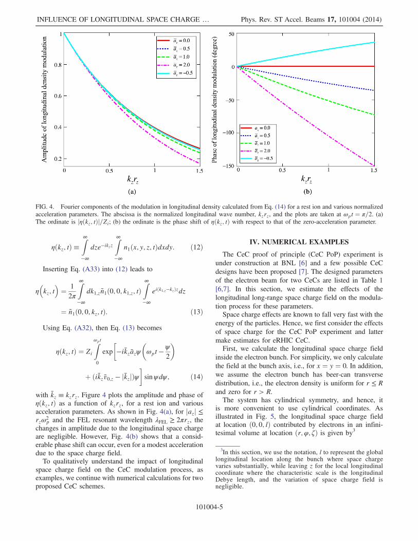
with kz ≡ kzrz. Figure 4 plots the amplitude and phase ofηðkz; tÞ as a function of kzrz, for a rest ion and variousacceleration parameters. As shown in Fig. 4(a), for jazj ≤rzω2
p and the FEL resonant wavelength λFEL ≥ 2πrz, thechanges in amplitude due to the longitudinal space chargeare negligible. However, Fig. 4(b) shows that a consid-erable phase shift can occur, even for a modest accelerationdue to the space charge field.To qualitatively understand the impact of longitudinal
space charge field on the CeC modulation process, asexamples, we continue with numerical calculations for twoproposed CeC schemes.
IV. NUMERICAL EXAMPLES
The CeC proof of principle (CeC PoP) experiment isunder construction at BNL [6] and a few possible CeCdesigns have been proposed [7]. The designed parametersof the electron beam for two CeCs are listed in Table 1[6,7]. In this section, we estimate the effects of thelongitudinal long-range space charge field on the modula-tion process for these parameters.Space charge effects are known to fall very fast with the
energy of the particles. Hence, we first consider the effectsof space charge for the CeC PoP experiment and lattermake estimates for eRHIC CeC.First, we calculate the longitudinal space charge field
inside the electron bunch. For simplicity, we only calculatethe field at the bunch axis, i.e., for x ¼ y ¼ 0. In addition,we assume the electron bunch has beer-can transversedistribution, i.e., the electron density is uniform for r ≤ Rand zero for r > R.The system has cylindrical symmetry, and hence, it
is more convenient to use cylindrical coordinates. Asillustrated in Fig. 5, the longitudinal space charge fieldat location ð0; 0; lÞ contributed by electrons in an infini-tesimal volume at location ðr;φ; ζÞ is given by3
FIG. 4. Fourier components of the modulation in longitudinal density calculated from Eq. (14) for a rest ion and various normalizedacceleration parameters. The abscissa is the normalized longitudinal wave number, kzrz, and the plots are taken at ωpt ¼ π=2. (a)The ordinate is jηðkz; tÞj=Zi; (b) the ordinate is the phase shift of ηðkz; tÞ with respect to that of the zero-acceleration parameter.
3In this section, we use the notation, l to represent the globallongitudinal location along the bunch where space chargevaries substantially, while leaving z for the local longitudinalcoordinate where the characteristic scale is the longitudinalDebye length, and the variation of space charge field isnegligible.
INFLUENCE OF LONGITUDINAL SPACE CHARGE … Phys. Rev. ST Accel. Beams 17, 101004 (2014)
101004-5

ΔEzðl; r;φ; ζÞ ¼rðl − ζÞρðζÞθðR − rÞΔζΔrΔφ
4πε0½ðζ − lÞ2 þ r2�32 ; ð15Þ
where θðxÞ is the Heaviside step function with thedefinition
θðxÞ≡1; x ≥ 0
0 x < 0; ð16Þ
and ρðζÞ is the density of the electron charge in the beamframe for r ≤ R. Integrating Eq. (15) over the transversearea of the beam yields the space charge field at locationð0; 0; lÞ due to a longitudinal slice of electrons at longi-tudinal location ζ with width Δζ
ΔEzðl; ζÞ ¼ρðζÞΔζ2ε0
�l − ζ
jl − ζj −l − ζffiffiffiffiffiffiffiffiffiffiffiffiffiffiffiffiffiffiffiffiffiffiffiffiffiffi
ðl − ζÞ2 þ R2p �
: ð17Þ
To proceed, we assumed that the electrons’ chargedistribution at r ≤ R has the following form:
ρðζÞ ¼ Qe
πR2
1ffiffiffiffiffiffi2π
pσz
e− ζ2
2σ2z ; ð18Þ
whereQe is the total charge of the electron bunch, and σz isthe rms length of the electron bunch. Inserting Eq. (18) into(17) and then integrating over z yields the longitudinalspace charge field at the location ð0; 0; lÞ,
EzðlÞ ¼−Qeffiffiffi2
pπ
32ε0σ
2z
F
�lσz
;Rσz
�; ð19Þ
with
Fðζ; χÞ≡ e−ζ2
2
χ2
Z∞0
e−ξ2
2 sinhðζ · ξÞ�
ξffiffiffiffiffiffiffiffiffiffiffiffiffiffiffiξ2 þ χ2
p − 1
�dξ:
ð20Þ
We note that, as shown in Fig. 6, even though the valuesof R=σz varies by 2 orders of magnitude for the two caseslisted in Table 1, the peak values of Fðl=σz; R=σzÞ onlychange by a factor of 2. We numerically evaluated Eq. (19)for the CeC PoP parameters and plot the results in Fig. 10(blue); they show the maximal longitudinal space chargefield reaches about 1.5 KV=m.As detailed in the previous section, the effects of the
space charge relate to the normalized acceleration param-eter, az, which can be calculated as follows:
azðlÞ ¼−eEzðlÞmeβzωpðlÞ
¼ −eEzðlÞmerzð0Þω2
pð0Þe
l2
4σ2z ; ð21Þ
where
ωpð0Þ ¼ffiffiffiffiffiffiffiffiffiffiffiffiffiffiffiffiffiffiffiffiffiffiffiffiffiffiffiffiffiffi
jQejeffiffiffiffiffiffiffi2π3
pR2σzmeε0
sð22Þ
and
rzð0Þ ¼βv;z
ωpð0Þð23Þ
are the plasma frequency and the longitudinal Debye lengthat the center of the electron bunch. The plasma frequency atlocation l is
TABLE I. Electron beam parameters for two CeC systemsproposed in [7].
Parameter/CeC CeC PoP eRHIC CeC
Bunch charge, nC 3.8 10Bunch length, rms, beamframe, σz, m
0.252 6.3
Beam radius R, mm 1.2 0.35R=σz 4.76 × 10⁻³ 5.56 × 10⁻⁵Energy ðMeVÞ= γ 21.5=42 136.2=266Longitudinal Debye length at thebunch center, beam frame, μm
46.3 19.1
Plasma phase advance inmodulator, rad
π=2 π=2
FIG. 5. Illustration of our calculation of the longitudinal spacecharge field.
4 2 2 4l
z
3
2
1
1
2
3
F
FIG. 6. Plot of the F function for two R=σz parameters inTable 1 versus l=σz. Blue is for the CeC PoP case; magenta is foreRHIC CeC.
G. WANG, M. BLASKIEWICZ, AND V. N. LITVINENKO Phys. Rev. ST Accel. Beams 17, 101004 (2014)
101004-6

ωpðlÞ ¼ e− l2
4σ2zωpð0Þ: ð24Þ
Employing Eqs. (19) and (21), we obtain the expressionfor the normalized acceleration parameter as follows:
azðlÞ ¼R2
rzð0Þ · σze
l2
4σ2zF
�lσz
;Rσz
�: ð25Þ
Figure 7 plots the normalized acceleration parameteralong the electron bunch for the CeC PoP parameters,suggesting that it stays below 0.4 within �4σz of thebunch.The apparent growth of jazðlÞj at jlj=σz > 3 in Fig. 7
does not mean that the effects of space charge field on themodulation are stronger for electrons far away from thebunch’s center. In practice, the time of interaction t ¼φpð0Þ=ωpð0Þ is fixed, and not the local phase advances ofplasma oscillations φpðlÞ ¼ ωpðlÞt, with l being the dis-tance from the bunch’s center. Hence, to properly evaluatethe space charge effect at l ≠ 0, we must evaluateEq. (11) at
ωpðlÞt ¼ φpð0Þ expð−l2=4σ2l Þ: ð26Þ
Figure 8 illustrates the dependence of the density modu-lation on az as function of the phase of plasma oscillation,e.g., Eq. (26). It shows that at small phase advances, thedependence is very weak. It is apparent from Fig. 7 that azreaches a local extreme of jazj ∼ 0.34 at jzj=σz ≈ 1.6. At thislocation, the plasma frequency is 2 times smaller than that inthe beam’s center, and with φpð0Þ ¼ π=2 → φpð1.6σzÞ ≈π=4. Hence, the effect onthe peak density does not exceed10% for jazj∼0.34. In addition, at jzj=σz ≈ 1.6, the e-beam’speak current is about 1=4 of that in the center. Therefore, inthe FEL-based CeC, the FEL gain is turned off at this
location, and hence, this part of the beam does not effectivelyparticipate in the cooling process.To account for the variation of ωpðlÞ along the bunch,
while estimating the influences of the longitudinal space’scharge field on the efficiency of modulation, we rewriteEq. (14) in non-normalized variables:
ηðkz; t; lÞ ¼ ZiωpðlÞ
×Zt0
exp
�−ikzazðlÞ
�t − τ
2
�τ
þ ðikz · v0;z − jkzjβv;zÞτ�sinðωpðlÞτÞdτ; ð27Þ
and the space charge influences along the electron bunchcan be represented by the following quantities:
Δηampðkz; t; lÞ≡ jηðkz; t; lÞj − jη0ðkz; t; lÞjjη0ðkz; t; lÞj
ð28Þ
and
Δηphðkz; t; lÞ≡ arg½ηðkz; t; lÞ� − arg½η0ðkz; t; lÞ� ð29Þwhere
η0ðkz; t; lÞ ¼ ZiωpðlÞZt0
exp½ðikz · v0;z − jkzjβzÞτ�
× sinðωpðlÞtÞdτ ð30Þ
is the Fourier component in the absence of the space chargeeffects, i.e., az ¼ 0. Figure 9 plots the relative changes of
�4 �2 0 2 4�0.4
�0.2
0.0
0.2
0.4
Longitudinal location � rms bunch length
Nor
mal
ized
acce
lera
tion
para
met
er
FIG. 7. Normalized acceleration parameter due to space chargefield (for the CeC PoP parameters listed in Table 1) as function ofthe longitudinal coordinate within a bunch.
FIG. 8. Plots of the normalized density at z ¼ 0, x ¼ 0.1rx, andy ¼ 0.1ry as functions of az (horizontal axis), and φp ¼ ωpt(vertical axis) ωpt ¼ π. The distributions are normalized to theirvalues at az ¼ 0. The contour lines are spaced by 0.2.
INFLUENCE OF LONGITUDINAL SPACE CHARGE … Phys. Rev. ST Accel. Beams 17, 101004 (2014)
101004-7

ηðkz; t; lÞ calculated from Eqs. (28) and (29) for theexperimental proof of the CeC principle.As shown in Fig. 9(a), the reduction in amplitude of the
wave packets due to the longitudinal space charge effects atthe modulator is under 0.04%. However, Fig. 9(b) showsthat the phase change of the initial modulation will result inthe maximal wave packet phase shift of �6°. Since thereduction of the CeC efficiency is proportional to the cosineof phase shift, this effect would lower CeC efficiency byless than 0.6%.Compared with the CeC proof-of-principle experiment,
the longitudinal space charge fields for the eRHIC CeC aredramatically lower. In the eRHIC CeC scheme, the strengthof the space charge field peaks at 6.15 V=m and con-sequently, the peak value of az falls, to �0.003.
V. EFFECTS FROM THE BEAM PIPE
In reality, the electron bunch usually is enclosed by ametallic vacuum chamber, the walls of which can affect thelongitudinal field acting on the electrons. In this section, weconsider two effects from the wall: screening of thelongitudinal space charge field and wake field due to wallresistivity.For perfectly conducting wall and σz=b ≫ 1, the longi-
tudinal space charge field in terms of the beam framevariables is given by4 [8]
Eapp;zðzÞ ¼e
4πε0
�2 ln
�bR
�þ 1
�dλdz
; ð31Þ
where b is the beam pipe’s radius, and
λðzÞ ¼ − πR2
eρðzÞ ð32Þ
is the electron line’s number density. Inserting Eqs. (18)and (32) into Eq. (31) yields
Eapp;zðzÞ ¼Qe
4ffiffiffi2
pπ
32ε0σ
2z
�2 ln
�bR
�þ 1
�zσz
e− z2
2σ2z : ð33Þ
More generally, in the presence of a circular perfectlyconducting beam pipe, the on-axis longitudinal spacecharge field of an electron bunch with the distribution ofEq. (18) and arbitrary bunch length is given by thefollowing 1D integral (Appendix B):
Eexa;zð0; zÞ ¼ − Qe
ε0π2R
×Z∞0
e−k2z σ
2z
2
�I1ðkzRÞK0ðkzbÞ
I0ðkzbÞ
þ K1ðkzRÞ − 1
kzR
�sinðkzzÞdkz; ð34Þ
where InðxÞ and KnðxÞ are the modified Bessel functions.In Fig 10, we plot the space charge field calculated from
FIG. 9. Influences of the longitudinal space charge field on the Fourier components of the longitudinal density modulation at the FELresonant wavelength as a function of longitudinal location along the electron bunch. The ion is at rest, and the parameters from the proofof the CeC principle experiment are applied in generating these plots. The abscissa is the longitudinal location in units of rms bunchlength. (a) The relative change in percentage of the amplitude of the Fourier component calculated from Eq. (28); (b) the phase change ofFourier component in degrees, calculated from Eq. (29).
4We defined e≡ 1.602… × 10−19C across this article, which isdifferent from the definition in [8].
G. WANG, M. BLASKIEWICZ, AND V. N. LITVINENKO Phys. Rev. ST Accel. Beams 17, 101004 (2014)
101004-8

Eqs. (33) and (34) for the parameters of the proof of theCeC principle experiment; they show that the formulasagree well for the considered parameters. More importantly,this figure implies that the shielding effects from a perfectlyconducting beam pipe wall reduce by 36% the peak fieldfrom the longitudinal space charge.In practice, the wall of the beam pipe always has nonzero
resistivity. As an electron bunch passing through the beam
pipe, the longitudinal wake field due to the resistive wall isgenerated and acts on the electrons, in addition to the spacecharge field. The energy change of an electron due tolongitudinal resistive wall wake field can be calculatedfrom [9]
ΔEðtÞ ¼ −eVsðtÞ ð35Þ
where
VsðtÞ ¼ −Z∞−∞
WsðτÞIbðt − τÞdτ ð36Þ
is the wake potential generated by an electron bunch withinstantaneous current of IbðtÞ,
WsðτÞ ¼ddτ
θðτÞ Ls
2πb
ffiffiffiffiffiffiffiffiffiffiρwZ0
πcτ
r ð37Þ
is the longitudinal resistive wall wake potential, θðτÞ is theHeaviside step function as defined in Eq. (16), Ls isthe length of the considered structure, b is the radius ofthe beam pipe, Z0 is the impedance of the free space, and ρwis the resistivity of the wall. The longitudinal electric fieldaveraged over the structure can be calculated as
EsðtÞ ¼VsðtÞLs
: ð38Þ
For an electron bunch with the Gaussian longitudinalprofile
IbðtÞ ¼ I0e− t2
2σ2τ ; ð39Þ
FIG. 10. The longitudinal space charge field of an electronbunch in the free space (blue) and, inside a beam pipe (red andgreen) with inner radius of 2.54 cm. The blue curve is generatedusing Eq. (19) for an electron bunch in the free space, the redcurve is produced by the approximate formula, Eq. (33), for along electron bunch inside a beam pipe, and the green curve iscreated from the exact formula, Eq. (34), for an electron bunchwith arbitrary length inside a beam pipe. The parameters of theproof of CeC principle experiment are applied for all plots.
FIG. 11. Average longitudinal electric field due to longitudinal resistive wall impedance for the CeC proof of principle experiment(left) and the proposed eRHIC CeC parameters (right). The following parameters are applied in generating the plots: ρw ¼6.9 × 10⁻⁷Ωm and b ¼ 2.54 cm. It is worth noting that the bunch head is at negative t, i.e. towards the left of the plots.
INFLUENCE OF LONGITUDINAL SPACE CHARGE … Phys. Rev. ST Accel. Beams 17, 101004 (2014)
101004-9

Eqs. (36)–(39) yields
EsðtÞ ¼ − I0πb
ffiffiffiffiffiffiffiffiffiffiffiffiffiffiffiffiρwZ0ffiffiffi2
pστπc
sG
�tffiffiffi2
pστ
�; ð40Þ
where
GðxÞ≡Z∞0
ð1 − 4xξþ 4x2Þffiffiffiξ
pe−ðξ−xÞ2dξ: ð41Þ
Figure 11 shows the average longitudinal electric fielddue to nonzero resistivity of beam pipe wall for the twocases listed in Table 1. The maximal field is 75 V=m for theproof of CeC principle experiment, which is more than oneorder of magnitude less than the space charge field. For theeRHIC scheme, the maximal longitudinal field due toresistive wall impedance is 25 V=m, which is muchstronger than the longitudinal space charge field. Toestimate the effects of the resistive wall wake field tothe modulation process for eRHIC CeC, we insert Eq. (40)into Eq. (21) and obtain
azðlÞ ¼−eEsð− l
γecÞ
merzð0Þω2pð0Þ
· el2
4σ2l : ð42Þ
Figure 12 shows the normalized acceleration parameteras a function of the longitudinal location along theelectron bunch for the eRHIC CeC scheme. For electronswithin �3σz, the normalized accelerator parameter staysbelow 0.02. Figure 13 plots the relative change of theFourier component at the resonant wavelength of theproposed FEL amplifier, 423 nm, due to the resistive wallimpedance as calculated from Eqs. (28) and (29) for theeRHIC CeC scheme, indicating that the relative change ofthe amplitude is below 3 × 10⁻⁶ and the phase change isbelow 0.4°.
VI. SUMMARY AND DISCUSSION
In this work, we developed an analytical model to studythe effect of ion shielding in the presence of a uniform
FIG. 13. Influences of the resistive wall wake field on the Fourier component of the longitudinal density modulation at the FELresonant wavelength, λFEL ¼ 423 nm. The ion is at rest, and the parameters from eRHIC CeC scheme are applied. The abscissa is thelongitudinal location in units of rms bunch length. (a) The relative change in percentage of the amplitude of the Fourier componentcalculated from Eq. (28); (b) the phase change of Fourier component in degrees, calculated from Eq. (29).
FIG. 12. Normalized acceleration parameter due to resistivewall impedance as function of the longitudinal coordinate withina bunch. Parameters for eRHIC CeC scheme are applied.
G. WANG, M. BLASKIEWICZ, AND V. N. LITVINENKO Phys. Rev. ST Accel. Beams 17, 101004 (2014)
101004-10

electric field. The model assumes a uniform electron spatialdistribution and an anisotropic 3D velocity distribution. Weshowed that the modulation in electron density, induced bya moving ion, could be expressed as a 1D integral thatdepends upon both the ion’s velocity and the acceleration ofelectrons caused by the external field. A higher modulationof the electron’s peak density occurs when the accelerationof electrons is along the same direction of the ion velocitythan otherwise.We applied this model to the processes in the CeC
modulator in the presence of a longitudinal electric field. Itsuse is valid provided that the spatial extension ofthe electron bunch is much larger than the correspondingDebye length. As numerical examples, we estimatedinfluences of the longitudinal space charge field and theresistive wall wake field on the modulation processes inCeC used for the proof-of-principle experiment at BNL, aswell as for the proposed eRHIC CeC. For the CeC PoPexperiment, the longitudinal space charge field is dominant.Our estimations show that its effect on the modulationprocess is relatively mild and can reduce CeC efficiencyonly by subpercent. For the CeC scheme proposed foreRHIC, the longitudinal resistive wall wake dominates andthis analysis confirmed our early estimations that the effectsdue to longitudinal electric field are negligible.Depending on the specific design of the modulator,
impedances from other sources, such as beam positionmonitors, beam pipe transitions, flanges, and bellows, mayalso contribute significantly to the electric fields in themodulator and hence should be considered for a morerealistic estimate. The analysis in Sec. III shows that, inorder to avoid severe adverse effects on the modulationprocess, the net longitudinal electric field due to imped-ances in the modulator should not exceed meβv;zωp=e,
5
with ωp and βv;z being the electrons’ local angular plasmafrequency and longitudinal velocity spread in the comovingframe, respectively.It is straightforward to calculate the electron density
modulation in the presence of the transverse space chargefield from Eq. (11). The FEL amplifiers for the proof ofCeC principle experiment and the proposed eRHIC CeCwork on the diffraction dominated regime and the trans-verse mode with maximal growth rate, i.e. the fundamentalmode, determines the performance of the system. AlthoughEq. (14) suggests that the transverse electric field does notaffect the Fourier components of the electron currentmodulation, it can affect the transverse distribution ofthe modulation and hence the initial component of thefundamental mode. A complete analysis of such effects
requires a 3D model for the FEL amplifier and needs to befurther pursued.
ACKNOWLEDGMENTS
This work was supported by Brookhaven ScienceAssociates, LLC under Contract No. DE-AC02-98CH10886 with the U.S. Department of Energy.
APPENDIX A: ANALYTICAL SOLUTIONFOR κ − 2 VELOCITY DISTRIBUTION
To proceed from Eqs. (8) and (9), it is convenient tochange the independent variables, ~v and t, to a set of newones:
~u≡ ~v − ~at; ðA1Þ
and
τ≡ t: ðA2ÞWe denote the induced variation in the phase space densityin terms of the new variables as follows:
f1ð~x; ~u; τÞ≡ findð~x; ~uþ ~aτ; τÞ: ðA3Þ
With the new variables, the partial derivatives in Eq. (8)with respect to ~v and t can be rewritten as
∂∂t findð~x; ~v; tÞ
����~v¼ − ∂
∂~u f1ð~x; ~u; τÞ����τ
· ~aþ ∂∂τ f1ð~x; ~u; τÞj~u;
ðA4Þ
and
~a ·∂∂~v findð~x; ~v; tÞjt ¼ ~a ·
∂∂~u f1ð~x; ~u; τÞjτ: ðA5Þ
Inserting Eqs. (A4) and (A5) into Eq. (8) yields thelinearized Vlasov equation in the new variables:
∂∂τ f1ð~x; ~u; τÞ þ ð~uþ ~aτÞ· ∂∂~x f1ð~x; ~u; τÞ
þ eme
~∇ϕindð~x; τÞ·∂∂~u f0ð~uÞ ¼ 0. ðA6Þ
The Poisson equation, Eq. (9), can be rewritten simply as
∇2ϕindð~x; τÞ ¼ − 1
ε0
�Zieδð~xÞ − e
Z∞−∞
f1ð~x; ~u; τÞd3u�:
ðA7ÞMultiplying both sides of Eqs. (A6) and (A7) by
e−i~k·~x, and integrating over ~x gives their Fouriertransformation:
5This upper limit is obtained by requiring that the normalizedacceleration parameter stays below unity and should be consid-ered as a rough estimate. More precise analysis for a certain typeof impedance requires evaluation of Eq. (27).
INFLUENCE OF LONGITUDINAL SPACE CHARGE … Phys. Rev. ST Accel. Beams 17, 101004 (2014)
101004-11

∂∂τ ~f1ð~k; ~u; τÞ þ i~k · ð~uþ ~aτÞ ~f1ð~k; ~u; τÞ
¼ −i eme
~ϕindð~k; τÞ~k ·∂∂~u f0ð~uÞ; ðA8Þ
and
~ϕindð~k; τÞ ¼e
ε0k2½Zi − ~n1ð~k; τÞ�: ðA9Þ
The Fourier components of the phase space density andelectric potential are defined as
~f1ð~k; ~u; τÞ ¼Z∞−∞
f1ð~x; ~u; τÞe−i~k·~xd3x; ðA10Þ
~ϕindð~k; τÞ ¼Z∞−∞
ϕindð~x; τÞe−i~k·~xd3x; ðA11Þ
and the Fourier components of the modulation in spatialdensity is given by
~n1ð~k; τÞ ¼Z∞−∞
~f1ð~k; ~u; τÞd3u: ðA12Þ
Multiplying both sides of Eq. (A8) by expði~k · ~uτþi~k · ~a τ2
2Þ, it becomes
∂∂τ
�ei~k·ð~uþ
~aτ2Þτ ~f1ð~k; ~u; τÞ
�
¼ −i eme
�~k ·
∂∂~u f0ð~uÞ
�ei~k·ð~uþ
~aτ2Þτ ~ϕindð~k; τÞ; ðA13Þ
that, after integration over τ, produces
~f1ð~k; ~u; τÞ ¼ −i eme
Zτ0
~ϕindð~k; τ1Þei~k·~aðτ2
1−τ2Þ
2
�~k ·
∂∂~u f0ð~uÞ
�
× ei~k·~uðτ1−τÞdτ1: ðA14Þ
Inserting Eq. (A9) into (A14), and then taking theintegration over ~u, leads to the following integral equation
~n1ð~k; τÞ ¼e2
ε0me
Zτ0
dτ1
�~n1ð~k; τ1Þ − Zi
�
× ei~k·~aðτ2
1−τ2Þ
2
Z∞−∞
�i~kk2
·∂∂~u f0ð~uÞ
�ei~k·~uðτ1−τÞd3u:
ðA15Þ
To move further, we assume that the initial distribution ofthe velocity of electrons at t ¼ 0 is an anisotropic κ-2distribution, which, in terms of the new variables, gives thedistribution of background electrons as follows:
f0ð~uÞ ¼n0
π2βv;xβv;yβv;z
×
�1þðuxþ v0xÞ2
β2v;xþðuyþ v0yÞ2
β2v;yþðuzþ v0zÞ2
β2v;z
�−2;
ðA16Þ
where ~v0 is the velocity of the ion, and n0 is the spatialdensity of the background electrons. Parameters βv;x, βv;y,and βv;z describe the velocity spreads of electrons in thecorresponding directions. Inserting Eq. (A16) into (A15)and applying the relation
iZ∞−∞
ei~k·~uτ~kk2
·∂∂~u f0ð~uÞd
3u ¼Z∞−∞
f0ð~uÞei~k·~uττd3u; ðA17Þ
the integral equation is reduced to
~n1ð~k; τÞ
¼ ω2p
Zτ0
½ ~n1ð~k; τ1Þ − Zi�ei~k·~aðτ2
1−τ2Þ
2 ðτ1 − τÞgð~kðτ − τ1ÞÞdτ1
¼ ω2p
Zτ0
½ ~n1ð~k; τ1Þ − Zi�ei~k·~aðτ2
1−τ2Þ
2 ðτ1 − τÞeλð~kÞðτ−τ1Þdτ1;
ðA18Þ
where
gð~qÞ≡ 1
n0
Z∞−∞
f0ð~uÞe−i~q·~ud3u
¼ exphi~q · ~v0 −
ffiffiffiffiffiffiffiffiffiffiffiffiffiffiffiffiffiffiffiffiffiffiffiffiffiffiffiffiffiffiffiffiffiffiffiffiffiffiffiffiffiffiffiffiffiffiffiq2xβ2v;x þ q2yβ2v;y þ q2zβ2v;z
q i; ðA19Þ
λð~kÞ≡ i~k · ~v0 −ffiffiffiffiffiffiffiffiffiffiffiffiffiffiffiffiffiffiffiffiffiffiffiffiffiffiffiffiffiffiffiffiffiffiffiffiffiffiffiffiffiffiffiffiffiffik2xβ2v;x þ k2yβ2v;y þ k2zβ2v;z
q; ðA20Þ
and,
G. WANG, M. BLASKIEWICZ, AND V. N. LITVINENKO Phys. Rev. ST Accel. Beams 17, 101004 (2014)
101004-12

ωp ≡ffiffiffiffiffiffiffiffiffiffin0e2
meε0
s: ðA21Þ
Equation (A18) can be written into a more compactform:
~H1ð~k; τÞ ¼ ω2p
Zτ0
�~H1ð~k; τ1Þ − Zie
i~k·~aτ21
2−λð~kÞτ1
�ðτ1 − τÞdτ1;
ðA22Þand, the new function, ~H1ð~k; τÞ, is defined as
~H1ð~k; τÞ≡ ~n1ð~k; τÞe−λð~kÞτþi~k·~aτ22 : ðA23Þ
Taking the second-time derivative of Eq. (A22) generatesan inhomogeneous second-order ordinary differentialequation
d2
dτ2~H1ð~k; τÞ þ ω2
p~H1ð~k; τÞ ¼ Ziω
2pe
i~k·~aτ22
−λð~kÞτ; ðA24Þ
which, for arbitrary initial conditions, has the solution [10]
~H1ð~k; τÞ ¼ c1 cosðωpτÞ þ c2 sinðωpτÞ
þ Ziωp
Zτ0
sin½ωpðτ − τ1Þ�ei~k·~aτ2
12
−λð~kÞτ1dτ1;
ðA25Þwith c1 and c2 being constants to be determined by theinitial conditions at t ¼ 0. As we assume that there is nomodulation at t ¼ 0, the initial conditions read
~H1ð~k; 0Þ ¼ ~n1ð~k; 0Þ ¼ 0; ðA26Þ
and
ddτ
~H1ð~k; τÞjτ¼0
¼ ddτ
~n1ð~k; τÞjτ¼0
− λð~kÞ ~n1ð~k; 0Þ ¼ 0.
ðA27Þ
Applying the initial conditions of Eq. (A26) to Eq. (A25)for τ ¼ 0 yields
c1 ¼ 0. ðA28Þ
Inserting Eq. (A28) into (A25) and then taking the first-time derivative produces
ddτ
~H1ð~k;τÞ¼ c2ωp cosðωpτÞþZiω2p cosðωpτÞ
×Zτ0
cosðωpτ1Þei~k·~aτ2
12
−λð~kÞτ1dτ1þZiω2p sinðωpτÞ
×Zτ0
sinðωpτ1Þei~k·~aτ2
12
−λð~kÞτ1dτ1: ðA29Þ
Equations (A27) and (A29) require
c2 ¼ 0; ðA30Þand hence, we obtain from Eqs. (A25), (A28), and (A30)
~H1ð~k; τÞ ¼ Ziωp
Zτ0
sin½ωpðτ − τ1Þ�e−λð~kÞτ1þi~k·~aτ2
12 dτ1:
ðA31Þ
Substituting the definition of ~H1ð~k; τÞ, Eq. (A23), backinto Eq. (A31), we obtain the modulation in electrondensity in the wave-vector domain
~n1ð~k; τÞ ¼ Ziωp
Zτ0
sin½ωpðτ − τ1Þ�eλð~kÞðτ−τ1Þ−i~k·~aðτ2−τ2
1Þ
2 dτ1:
ðA32Þ
The electron-density modulation in the configurationspace is given by the inverse Fourier transformation of
~n1ð~k; τÞ, i.e.,
n1ð~x; tÞ ¼1
ð2πÞ3Z∞−∞
~n1ð~k; tÞei~k·~xd3k: ðA33Þ
Inserting Eq. (A32) into Eq. (A33), we finally obtain thefollowing expression for the electron-density modulationinduced by an ion:
n1ð~x; tÞ ¼Zi
π2rxryrz
Zωpt
0
ψ sinψ
�ψ2 þ
�x − axψ
�ωpt − ψ
2
�þ v0;xψ
�2
þ�y − ayψ
�ωpt − ψ
2
�þ v0;yψ
�2
þ�z − azψ
�ωpt − ψ
2
�þ v0;zψ
�2�−2
dψ ; ðA34Þ
wherein we used the normalized variables, defined as xj ≡ xj=rj, aj ≡ aj=rjω2p, v0;j ¼ v0;j=βv;j, and rj ≡ βv;j=ωp, with the
index, j ¼ x; y; z, referring to the components of a spatial vector.
INFLUENCE OF LONGITUDINAL SPACE CHARGE … Phys. Rev. ST Accel. Beams 17, 101004 (2014)
101004-13

APPENDIX B: LONGITUDINAL SPACE CHARGEFIELD OF A CHARGED BUNCH INSIDE A
CONDUCTING CIRCULAR PIPE
For a charged particle bunch enclosed by an infinitelylong conducting beam pipe with radius b, the electricpotential, φ, at the beam pipe is equal to its value at infinity,such that the boundary condition can be set as
φðb;ϕ; zÞ ¼ φðr;ϕ;∞Þ ¼ 0. ðB1Þ
We assume that the charged-particle bunch is trans-versely uniform with radius R and its total charge is Qe. Inthe comoving frame of the bunch, the Poisson equationinside the beam pipe reads
∇2φ ¼ − Qe
ε0πR2
1ffiffiffiffiffiffi2π
pσz
e− z2
2σ2zθðR − rÞ; ðB2Þ
where θðxÞ is the Heaviside step function with thedefinition
θðxÞ≡1; x ≥ 0
0; x < 0: ðB3Þ
In cylindrical coordinates, Eq. (B2) becomes
1
r∂∂r
�r∂∂r
�φþ 1
r2∂2
∂ϕ2φþ ∂2
∂z2 φ
¼ − Qe
ε0πR2
1ffiffiffiffiffiffi2π
pσz
e− z2
2σ2zθðR − rÞ: ðB4Þ
Since the system has cylindrical symmetry, the derivativewith respect to the azimuthal angle, ϕ, vanishes, and hence,Eq. (B4) reduces to
1
r∂∂r
�r∂∂r
�φþ ∂2
∂z2 φ ¼ − Qe
ε0πR2
1ffiffiffiffiffiffi2π
pσz
e− z2
2σ2zθðR − rÞ:
ðB5Þ
Taking Fourier transformation of Eq. (B5) along the zaxis yields the following:
1
r∂∂r
�r∂∂r
�~φinðr; kzÞ − k2z ~φinðr; kzÞ
¼ − Qe
ε0πR2e−
k2z σ2z
2 θðR − rÞ; ðB6Þ
where
~φðr; kzÞ≡Z∞−∞
e−ikzφðr; zÞdz: ðB7Þ
The boundary condition for ~φðr; kzÞ at r ¼ b is obtainedfrom Eqs. (B1) and (B7) as
~φðb; kzÞ ¼ 0. ðB8Þ
Expanding the first term of Eq. (B6) yields
∂2
∂r2 ~φinðr; kzÞ þ1
r∂∂r ~φinðr; kzÞ − k2z ~φinðr; kzÞ
¼ − Qe
ε0πR2e−
k2z σ2z
2 θðR − rÞ: ðB9Þ
For r ≤ R, Eq. (B9) can be rewritten into
∂2
∂ ~r2 ~φinð~r; kzÞ þ1
~r∂∂ ~r ~φinð~r; kzÞ − ~φinð~r; kzÞ
¼ − Qe
ε0πk2zR2e−
k2z σ2z
2 ; ðB10Þ
with
~r ¼ kzr: ðB11Þ
Equation (B10) is the inhomogeneous modified Besseldifferential equation, and its solution can be expressed as
~φinð~r; kzÞ ¼ ~φin;hð~r; kzÞ þ ~φin;pð~r; kzÞ; ðB12Þ
where
~φin;hð~r; kzÞ ¼ c1ðkzÞI0ð~rÞ þ c2ðkzÞK0ð~rÞ ðB13Þ
is the solution of the homogeneous modified Besseldifferential equation, i.e.,
∂2
∂ ~r2 ~φin;hð~r; kzÞ þ1
~r∂∂ ~r ~φin;hð~r; kzÞ − ~φin;hð~r; kzÞ ¼ 0;
ðB14Þand ~φin;pðkz; ~rÞ is the particular solution satisfyingEq. (B10). Since the driving term in Eq. (B10) is inde-pendent of ~r, the particular solution reads
~φin;pð~r; kzÞ ¼Qe
ε0πk2zR2e−
k2z σ2z
2 : ðB15Þ
Inserting Eqs. (B13) and (B15) into eq. (B12) yields
~φinð~r; kzÞ ¼ c1ðkzÞI0ð~rÞ þ c2ðkzÞK0ð~rÞ þQe
ε0πk2zR2e−
k2z σ2z
2 :
ðB16Þ
G. WANG, M. BLASKIEWICZ, AND V. N. LITVINENKO Phys. Rev. ST Accel. Beams 17, 101004 (2014)
101004-14
Requiring ~φinð~r ¼ 0Þ to being finite leads to
~φinð~r; kzÞ ¼ c1ðkzÞI0ð~rÞ þQe
ε0πk2zR2e−
k2z σ2z
2 : ðB17Þ
For r > R, Eq. (B9) becomes the homogeneous modifiedBessel differential equation
∂2
∂ ~r2 ~φoutð~r; kzÞ þ1
~r∂∂ ~r ~φoutð~r; kzÞ − ~φoutð~r; kzÞ ¼ 0;
ðB18Þ
that has solutions of the form
~φoutð~r; kzÞ ¼ d1ðkzÞI0ð~rÞ þ d2ðkzÞK0ð~rÞ: ðB19Þ
Applying the boundary condition, Eq. (B8), leads to
d2ðkzÞ ¼ −d1ðkzÞ I0ðkzbÞK0ðkzbÞ; ðB20Þ
and hence, Eq. (B19) becomes
~φoutð~r; kzÞ ¼ d1ðkzÞ�I0ð~rÞ − I0ðkzbÞ
K0ðkzbÞK0ð~rÞ
�: ðB21Þ
The two remaining coefficients, c1ðkzÞ and d1ðkzÞ, aredetermined by the conditions at the beam’s boundary,r ¼ R, which read
~φoutðkzR; kzÞ ¼ ~φinðkzR; kzÞ; ðB22Þ
and
∂∂ ~r ~φoutð~r; kzÞ
����~r¼kzR; kz¼const
¼ ∂∂ ~r ~φinð~r; kzÞ
����~r¼kzR; kz¼const
:
ðB23Þ
Eqs. (B22) and (B23) produce
d1ðkzÞ ¼ − Qe
ε0πkzR2
RI1ðkzRÞK0ðkzbÞI0ðkzbÞ
e−k2z σ
2z
2 ; ðB24Þ
and
c1ðkzÞ ¼ − Qe
ε0πkzRe−
k2z σ2z
2
�I1ðkzRÞ
K0ðkzbÞI0ðkzbÞ
þ K1ðkzRÞ�;
ðB25Þ
where we used the relations
ddz
K0ðzÞ ¼ −K1ðzÞ; ðB26Þ
and
ddz
I0ðzÞ ¼ I1ðzÞ; ðB27Þ
and
IνðzÞKνþ1ðzÞ þ Iνþ1ðzÞKνðzÞ ¼1
z: ðB28Þ
Inserting Eqs. (B24) and (B25) into Eqs. (B21) and(B17) generates
~φinðr; kzÞ
¼ − Qe
ε0πR2e−
k2z σ2z
2
×
Rkz
�I1ðkzRÞK0ðkzbÞ þ K1ðkzRÞI0ðkzbÞ
I0ðkzbÞ�
× I0ðkzrÞ − 1
k2z
; ðB29Þ
for r ≤ R, and
~φoutðr; kzÞ ¼ − QeRε0πkzR2
e−k2z σ
2z
2I1ðkzRÞI0ðkzbÞ
× ½K0ðkzbÞI0ðkzrÞ − I0ðkzbÞK0ðkzrÞ�; ðB30Þ
for R < r ≤ b.The electric potential inside the bunch is given by the
inverse Fourier transformation of Eq. (B29), i.e.,
φinðr; zÞ ¼1
2π
Z∞−∞
~φinðr; kzÞeikzzdkz; ðB31Þ
that leads to the longitudinal electric field,
Ez;inðr; zÞ ¼ − ∂∂zφinðr; zÞ ¼ − i
2π
Z∞−∞
kz ~φinðr; kzÞeikzzdkz:
ðB32Þ
On the bunch axis, r ¼ 0, and the longitudinal electricfield is
INFLUENCE OF LONGITUDINAL SPACE CHARGE … Phys. Rev. ST Accel. Beams 17, 101004 (2014)
101004-15

Ez;inð0; zÞ ¼ − i2π
Z∞−∞
kz ~φinð0; kzÞeikzzdkz ¼Qe
ε0πRi2π
Z∞−∞
e−k2z σ
2z
2
I1ðkzRÞK0ðkzbÞ
I0ðkzbÞþ K1ðkzRÞ − 1
kzR
eikzzdkz
¼ Qe
ε0πRi2π
Z∞0
½fðkzÞeikzz þ fð−kzÞe−ikzz�dkz; ðB33Þ
with
fðkzÞ¼ e−k2z σ
2z
2
I1ðkzRÞK0ðkzbÞþ I0ðkzbÞK1ðkzRÞ
I0ðkzbÞ− 1
kzR
:
ðB34Þ
The function, fðkzÞ, is an odd function of kz. To prove it,it is sufficient to show that the function
hðkzÞ ¼ I1ðkzRÞK0ðkzbÞ þ I0ðkzbÞK1ðkzRÞ ðB35Þ
is odd, or, more explicitly,
hðkzÞ þ hð−kzÞ ¼ I1ðkzRÞ½K0ðkzbÞ − K0ð−kzbÞ�þ I0ðkzbÞ½K1ðkzRÞ þ K1ð−kzRÞ�;
ðB36Þ
vanishes for any real value of kz. The integral representa-tions of the modified Bessel function of the 0th zeroth orderread [11]
K0ðzÞ ¼ − 1
π
Zπ0
e�z cos θ½γ þ lnð2zsin2θÞ�dθ; ðB37Þ
and
I0ðzÞ ¼1
π
Zπ0
e�z cos θdθ; ðB38Þ
where
γ ≡ limn→∞
�1þ 1
2þ 1
3þ � � � þ 1
n− ln n
�≈ 0.5772156649… ðB39Þ
is the Euler’s constant. It follows from Eq. (B37) that
K0ðzÞ − K0ð−zÞ ¼ − 1
π
Zπ0
e�z cos θ½lnð2zsin2θÞ − lnð−2zsin2θÞ�dθ ¼ lnð−1Þπ
Zπ0
e�z cos θdθ ¼ iπð2nþ 1ÞI0ðzÞ; ðB40Þ
with n being an arbitrary integer. Taking the first derivative of Eq. (B40) gives
K1ðzÞ þ K1ð−zÞ ¼ −iπð2nþ 1ÞI1ðzÞ: ðB41Þ
Using Eqs. (B40) and (B41), Eq. (B36) becomes
hðkzÞ þ hð−kzÞ ¼ iπð2nþ 1ÞI1ðkzRÞI0ðkzbÞ − iπð2nþ 1ÞI1ðkzRÞI0ðkzbÞ ¼ 0; ðB42Þ
and consequently, we proved that fðkzÞ is an odd function, i.e.,
fð−kzÞ ¼ −fðkzÞ: ðB43ÞInserting Eq. (B43) into Eq. (B33), we obtain
Ez;inð0; zÞ ¼ − Qe
ε0π2R
Z∞0
fðkzÞ sinðkzzÞdkz ¼ − Qe
ε0π2R
Z∞0
e−k2z σ
2z
2
I1ðkzRÞK0ðkzbÞ
I0ðkzbÞþ K1ðkzRÞ − 1
kzR
sinðkzzÞdkz:
ðB44Þ
G. WANG, M. BLASKIEWICZ, AND V. N. LITVINENKO Phys. Rev. ST Accel. Beams 17, 101004 (2014)
101004-16

It often is convenient to express Eq. (B44) in terms of thenormalized variables
Ez;inð0; zÞ ¼ − Qe
ε0π2Rσ2z
Z∞0
e−ξ2
2
I1ðξ · RÞK0ðξ · bÞ
I0ðξ · bÞ
þ K1ðξ · RÞ − 1
ξR
sinðξ · zÞdξ; ðB45Þ
with R ¼ R=σz, z ¼ z=σz, and b ¼ b=σz. Applying theasymptotic behavior of the modified Bessel function atkz → 0 yields
limkz→0
½fðkzÞ sinðkzzÞ� ¼ limkz→0
�− kzR
2lnðkzbÞ
þ 1
kzR− 1
kzR
�sinðkzzÞ
¼ 0.
ðB46Þ
At kz → ∞, the asymptotic behaviors of the modifiedBessel functions are
I0;1ðxÞ ∼exffiffiffiffiffiffiffiffi2πx
p ;
K0;1ðxÞ ∼ffiffiffiffiffiπ
2x
re−x;
and hence, it follows that
limkz→∞
½fðkzÞ sinðkzzÞ� ¼ limkz→∞
e−
k2z σ2z
2
� ffiffiffiffiffiffiffiffiffiffiπ
2kzR
re−kzð2b−RÞ
þffiffiffiffiffiffiffiffiffiffiπ
2kzR
re−kzR − 1
kzR
�sinðkzzÞ
¼ 0. ðB47Þ
Equations (B46) and (B47) suggest that the integrand ofthe integral in Eq. (B44) is a finite real function. Figure 14compares the results in Eq. (B44) with the previouslyderived longitudinal space charge field in the absence of thebeam pipe and with that in the presence of the beam pipebut with long beam approximation. As shown in Fig. 14(a),when the beam frame’s bunch length, 1.26 cm, is muchsmaller than the beam pipe’s radius, the exact solution(green) in Eq. (B44) overlaps with that for an open beam(blue), i.e., without a beam pipe. Figure 14(b) shows that asthe beam frame’s bunch length increases to 1.26 m, theexact solution overlaps with that of the long-bunchapproximation (red). With a rms bunch length of 5 cm,Fig. 14(c) shows that the exact solution deviates from thatin both of the other solutions.
[1] Ya. S. Derbenev, in Proceedings of the 7th Conference onCharged Particle Accelerators, Dubna, USSR, 1980, p. 269[http://ab‑abp‑clic‑qcde.web.cern.ch/ab‑abp‑clic‑qcde/Literature/Derbenev_1991_Coherent_Electron_Cooling.pdf]
FIG. 14. The exact longitudinal space charge field in the presence of the 5 cm radius beam pipe. The abscissas are the longitudinallocations in units of the rms bunch length and the ordinates are the longitudinal space charge field in units of V/m. The green dashedcurve shows the field calculated from the exact solution, i.e., Eq. (B44), the blue solid curve shows the field from the electron bunch,without considering the beam pipe, and the red solid curve shows the field calculated from an approximate formula where shielding fromthe beam pipe is considered but the electron bunch is assumed to be much longer than the beam pipe’s radius. (a) Calculated for PoPparameters but with 1.26 cm beam frame rms bunch length; (b) calculated with 1.26 m beam framerms bunch length;(c) calculated with5 cm beam frame rms bunch length.
INFLUENCE OF LONGITUDINAL SPACE CHARGE … Phys. Rev. ST Accel. Beams 17, 101004 (2014)
101004-17

[2] V. N. Litvinenko and Ya. S. Derbenev, in Proceedings ofthe 29th International Free Electron Laser Conference,FEL-2007, Novosibirsk, Russia (JACoW, Novosibirsk,Russia, 2007), p. 268 [http://accelconf.web.cern.ch/AccelConf/f07/PAPERS/TUCAU01.PDF].
[3] V. N. Litvinenko and Y. S. Derbenev, Phys. Rev. Lett. 102,114801 (2009).
[4] D. Ratner, Phys. Rev. Lett. 111, 084802 (2013).[5] G. Wang and M. Blaskiewicz, Phys. Rev. E 78, 026413
(2008).[6] I. Pinayev et al., in Proceedings of the 4th International
Particle Accelerator Conference, IPAC-2013, Shanghai,China, 2013 (JACoW, Shanghai, China, 2013), p. 1535.
[7] V. N. Litvinenko, in Proceedings of the InternationalWorkshop on Beam Cooling and Related Topics,COOL’13, Mürren, Switzerland, 2013 (JACoW, Mürren,Switzerland, 2013), p. 175 [http://accelconf.web.cern.ch/AccelConf/COOL2013/papers/tham2ha02.pdf].
[8] S.-Y. Lee, Accelerator Physics (World Scientific, Singapore,2004).
[9] M. Blaskiewicz, http://www.bnl.gov/isd/documents/32667.pdf.
[10] I. Gradshteyn and I. Ryzhik, Tables of Integrals, Series andProducts, 7th ed. (Academic Press, New York, 2007).
[11] M. Abramowitz, National Bureau of Standards AppliedMathematics Series 55, 376 (1965).
G. WANG, M. BLASKIEWICZ, AND V. N. LITVINENKO Phys. Rev. ST Accel. Beams 17, 101004 (2014)
101004-18