inflation targeting and fiscal rules in developing
TRANSCRIPT
HAL Id: tel-01167687https://tel.archives-ouvertes.fr/tel-01167687
Submitted on 24 Jun 2015
HAL is a multi-disciplinary open accessarchive for the deposit and dissemination of sci-entific research documents, whether they are pub-lished or not. The documents may come fromteaching and research institutions in France orabroad, or from public or private research centers.
L’archive ouverte pluridisciplinaire HAL, estdestinée au dépôt et à la diffusion de documentsscientifiques de niveau recherche, publiés ou non,émanant des établissements d’enseignement et derecherche français ou étrangers, des laboratoirespublics ou privés.
Inflation targeting and fiscal rules in developingcountries : interactions and macroeconomic consequences
René Tapsoba
To cite this version:René Tapsoba. Inflation targeting and fiscal rules in developing countries : interactions and macroe-conomic consequences. Economics and Finance. Université d’Auvergne - Clermont-Ferrand I, 2012.English. �NNT : 2012CLF10394�. �tel-01167687�

Université d’Auvergne, Clermont-Ferrand 1
Faculté des Sciences Économiques et de Gestion
École Doctorale des Sciences Économiques, Juridiques et de Gestion
Centre d’Études et de Recherches sur le Développement International (CERDI)
Inflation Targeting and Fiscal Rules in Developing
Countries: Interactions and Macroeconomic Consequences
Thèse Nouveau Régime Présentée et soutenue publiquement le 25 Juin 2012
Pour l’obtention du titre de Docteur ès Sciences Économiques
Par
René TAPSOBA
Sous la direction de:
M. Le Professeur Jean-Louis COMBES M. Le Professeur Alexandru MINEA
Membres du Jury:
Jean-Bernard CHATELAIN, Professeur, Université Paris 1, Panthéon Sorbonne (Rapporteur)
Marc-Alexandre SENEGAS, Professeur, Université Montesquieu Bordeaux IV (Rapporteur)
Nasser ARY TANIMOUNE, Professeur Adjoint, School of International Development and
Global Studies, University of Ottawa (Suffragant)
Xavier DEBRUN, Deputy Division Chief at the Fiscal Affairs Department, International Monetary Fund (Suffragant)
Patrick VILLIEU, Professeur, Directeur du Laboratoire d’Economie d’Orléans (Suffragant)
Jean-Louis COMBES, Professeur, Université d’Auvergne, CERDI (Directeur de thèse)
Alexandru MINEA, Professeur, Université d’Auvergne, CERDI (Directeur de thèse)


La faculté n’entend donner aucune approbation ou improbation aux opinions émises dans
la thèse. Ces opinions doivent être considérées comme propres à leur auteur.

À mes parents, Mathias et Noëllie,
À mes frères et sœurs, Romuald, Pierre et Denise


Remerciements - Acknowledgments
Avant tout propos, je tiens à traduire toute ma gratitude à l’endroit de tous ceux et de toutes celles, qui,
d’une manière ou d’une autre, ont permis l’aboutissement heureux de cette thèse. Je pense en
particulier à Messieurs les Professeurs Jean-Louis Combes et Alexandru Minea qui ont eu l’amabilité
d’accepter de diriger mes travaux durant ces trois années. J’ai beaucoup apprécié de travailler sous
votre encadrement empreint de rigueur, de suivi régulier et de bienveillance. Je puis vous assurer que
j’ai énormément appris à vos côtés.
L’expression de ma profonde gratitude s’adresse également aux Professeurs Jean-Bernard Chatelain,
Marc-Alexandre Senegas, Patrick Villieu, et à Messieurs les Docteurs Nasser Ary Tanimoune et
Xavier Debrun pour avoir généreusement accepté d’être membres de ce Jury de Thèse, témoignant
ainsi leur intérêt pour mes travaux.
Cette thèse doit également beaucoup au Ministère Français de l’Enseignement Supérieur et de la
Recherche, qui au travers de l’Université d’Auvergne, m’a gratifié d’un financement, lequel a
considérablement facilité sa rédaction. De même, l’excellence des conditions de travail du CERDI
ainsi que la qualité des enseignements dont j’ai bénéficiés durant mes trois années de Magistère sont
bien sûr le socle sur lequel je me suis appuyé pour l’écriture de cette thèse. La gentillesse et le
dynamisme de tout le personnel administratif ont également favorisé mon épanouissement dans ma vie
de doctorant. Puissent-toutes ces personnes trouver à travers ces lignes mes sincères remerciements.
Pour la rédaction du Chapitre 7 de la thèse, j’ai effectué un séjour de recherche à l’Ecole de
Développement International et de Mondialisation de l’Université d’Ottawa. A cet égard, j’ai bénéficié
d’un financement conjoint de la Fondation de l’Université d’Auvergne et de l’Université d’Ottawa.
Merci infiniment à ces deux entités pour leurs générosités à mon égard. J’aimerais aussi remercier
chaleureusement M. Ary Tanimoune Nasser pour l’excellence de l’accueil dont il m’a fait montre à
cette occasion. Je voudrais également remercier sincèrement tous les participants aux séminaires et
conférences auxquels j’ai pris part, pour leurs commentaires pertinents. Merci également à Samuel
Guérineau, Chloé Duvivier, Florian Léon, Yannick Lucotte et Achille Souilli pour toutes les fois où ils
ont généreusement relu cette thèse.

J’ai naturellement une pensée spéciale à mes très sympathiques promotionnaires de thèse (Alexandre,
Aurore, Céline, Charline, Chloé, Eric, Mireille, Moussa, Yep et Zorobabel) et plus généralement à mes
camarades de classe du Magistère, pour l’ambiance combien conviviale qu’ils ont su instaurer durant
ces six années « cerdiennes ». Rassurez-vous, j’en garderai de très beaux souvenirs! Un merci très
spécial à Zorobabel dit « Zoro le Justicier », mon co-auteur de toujours: tout en te souhaitant bonne
chance dans ta thèse, je te renouvelle mes remerciements pour ta fraternité!
Je pense aussi à mes illustres devanciers sur le chemin du doctorat, pour tous leurs conseils avisés:
Christian Ebéké, Yacouba Gnégné, Jules-Armand Tapsoba, Tidiane Kinda, Ulrich Zombré, Alassane
Drabo, Thierry Kangoye, Romuald Kinda, Gaoussou Diarra, Yannick Lucotte, Félix Badolo, Seydou
Ouédraogo, Luc Désiré Omgba, Fousseini Traoré, Eric Djimeu, Seydou Dao, Hélène, Emilie
Catherine et Sébastien. Je remercie aussi mes jeunes frères doctorants (Moussé, Samba, Youssouf,
Christian, Florian, Antoine, Gwenolee). Je pense également aux doctorants avec qui j’ai
chaleureusement co-assuré les travaux dirigés à la Faculté (Chloé, Thierry, Gaoussou, Florian,
Gwenolee, Sébastien, Alassane).
La saine émulation de ma vie de doctorant est également beaucoup redevable à la dynamique équipe
de football du CERDI, au sein de laquelle j’ai livré des matchs de haut niveau qui resteront à jamais
gravés dans ma mémoire. Merci aux vaillants co-équipiers avec qui j’ai partagé ces beaux moments.
Comme on le dit si souvent, « La musique adoucit les mœurs!». J’adresse ainsi une pensée spéciale à
mes camarades de la Chorale Africaine Chœur des Anges, avec qui j’ai toujours pris du plaisir à
fredonner des belles et adoucissantes mélodies pendant ces années à Clermont. Mes camarades de la
vie Associative ne sont pas en reste. Je pense aux membres de l’Association des Burkinabès de
Clermont-Ferrand (ABUC). Je remercie aussi mes amis qui m’ont toujours apporté leur soutien (Juste
A. Goungounga, Romain C. Ouédraogo, Martin Kanazoé, Gilbert Korogho, Ulrich Zombré, Gislain
Zombré, Yves Kinda, Patrice Zidouemba, David Zombré, Gilles Koala, Yves Koala, Rémi Tapsoba,
Nafissatou, Inès, Saïdou, Martin Simporé, Romaric Ouédraogo, Missom G. Benoît, Valentin Ilboudo,
Eric Kinda, Hyacinthe Nikièma, Irmeya Ouédraogo, Marcel Thiombiano, Jean-Abel Traoré, Jean-Luc
Kafando, Hervé Yamkoudougou, Dieudonné Kaboré et Paul Conseiga). La contrainte d’espace
m’oblige à conclure ici la liste des remerciements; mes sincères excuses donc à tous ceux et à toutes
celles qui ne verraient pas leurs noms! Rassurez-vous, ceci n’est point synonyme d’un manque de
reconnaissance à l’égard de nos relations cordiales, de notre camaraderie, amitié et fraternité.
Pour finir, j’aimerais rendre un hommage particulier à mes parents, mes frères et à ma sœur, qui n’ont
jamais douté de moi, et qui malgré la distance m’ont toujours soutenu. Mention spéciale à Olivia dont
la présence apaisante m’a inspiré et procuré un « second souffle » dans la dernière ligne droite de cette
thèse.


List of acronyms
AE Advanced Economy
ATT Average Treatment effect on the Treated
BBR(s) Budget Balance Rule(s)
CAB Cyclically-Adjusted overall fiscal Balance
CAPB Cyclically-Adjusted Primary fiscal Balance
CAPE Cyclically-Adjusted-Primary Expenditure
CEE Central and Eastern Europe
CEEC Central and Eastern European Countries
CEMAC Central African Economic and Monetary Community
CERDI Centre d’Etudes et de Recherches sur le Développement International
CFA Communauté Financière Africaine
CPI Consumer Price Index
DID Differences-in-Differences
DR(s) Debt Rule(s)
ECB European Central Bank
ECCU Eastern Caribbean Currency Union
ECOWAS Economic Community of West African States
EIT Eclectic Inflation Targeting
EME Emerging Market Economy
EMS European Monetary System
EMU Economic and Monetary Union of the European Union
ER(s) Expenditure Rule(s)
ERM Exchange Rate Mechanism
FB (Overall) Fiscal Balance
FD Fiscal Discipline
FDI Foreign Direct Investment
Fed Federal Reserve
FFIT Full-Fledged Inflation Targeting
FOC First Order Condition
FR(s) Fiscal Rule (s)

FRer Country having adopted fiscal rule (FR)
GDP Gross Domestic Product
GFS Government Financial Statistics
GMM Generalized Method of Moments
ICRG International Country Risk Guide
IFS International Financial Statistics
IMF International Monetary Fund
IT Inflation Targeting
ITer(s) Inflation Targeter(s): countries having adopted Inflation Targeting
ITL Inflation Targeting Lite
LIC Low Income Country
MCI Monetary Conditions Index
MP Monetary Policy
OECD Organization for Economic Co-operation and Development
OLS Ordinary Least Squares
PCE Personal Consumption Expenditure price index
PFB Primary Fiscal Balance
PFM Public Financial Management
PS Propensity Score
PSM Propensity Scores-Matching
PWT Penn World Table
QI Quality of Institutions
QOG Quality Of Government
REER Real Effective Exchange Rate
ROSC Reports on the Observance of Standards and Codes
RR(s) Revenue Rule(s)
SBS (Primary) Structural Fiscal Balance
SGP Stability and Growth Pact
UK United Kingdom
US United States (of America)
VAT Value Added Tax
WAEMU West African Economic and Monetary Union
WAMZ West African Monetary Zone
WDI World Development Indicators
WEO World Economic Outlook
2SLS Two Stages Least Squares


Table of Contents
General Introduction 1
Chapter 1: Definitions, Typology and Overview of Inflation Targeting and Fiscal Rule
Experiences Around the World 15
Chapter 2: Does Inflation Targeting Matter for Attracting Foreign Direct Investment
into Developing Countries? 57
Chapter 3: Can Inflation Targeting Promote Institutional Quality in Developing
Countries? 81
Chapter 4: Do National Numerical Fiscal Rules Really Shape Fiscal Behaviors in
Developing Countries? 115
Chapter 5: Does Inflation Targeting Improve Fiscal Discipline? 143
Chapter 6: Inflation Targeting and Fiscal Rules: Do Interactions and Sequence of
Adoption Matter? 179
Chapter 7: Policy Mix Coherence and Monetary Policy in West Africa 205
General Conclusion 223
References 233
Contents 251


1
GENERAL INTRODUCTION
“The primary usefulness of […] fiscal rules consists of establishing a depoliticized framework for fiscal policy – much like the depoliticization of monetary policy under
successful inflation targeting” (Kopits, 2001, p. 8)

General Introduction
2
ince the early 1990s, rules-based macroeconomic policy frameworks are gaining
considerable popularity among policymakers and academics around the world. On the
monetary area, Inflation Targeting (IT) emerged as the new framework for the conduct of
monetary policy (MP) while in the fiscal area, Fiscal Rules (FRs) turned out to be the
framework of reference for conducting fiscal policy soundly, away from political pressures.
Both frameworks (IT and FRs) function in the form of numerical targets placed officially and
durably on macroeconomic aggregates (inflation and fiscal variables for IT and FRs
respectively), - hence the term rules-based -, proceeds with ex-ante forecasts of these
aggregates, and are supported by institutional infrastructures – transparency and
accountability mechanisms inter alia - to frame the regular communications with the financial
markets and the general public, regarding the different policy objectives, stances and
decisions (see Bernanke and Mishkin, 1997; Svensson, 1999; Mishkin, 2000; Truman, 2003
for IT; and Von Hagen, 1992; Kopits & Symansky, 1998; Alesina et al.,1999 for FRs).1
According to the last IMF’s classification of MP frameworks, around 44 countries can be
considered as operating under IT.2 But given that this classification includes the member
States of the Economic and Monetary Union (EMU) of the European Union in the group of
Inflation Targeters (ITers) while there is no consensus that the European Central Bank (ECB)
practices IT, excluding these countries allows seeing that there are actually around 30
countries practicing explicitly IT.3 Besides the relative important number of countries having
adopted IT, another worth highlighting fact is that this new MP regime proliferated
worldwide, gaining the developed as well as the developing world. First adopted by the
Reserve Bank of New Zealand in 1990, IT rapidly spread among industrialized countries:
Bank of Canada (1991), the Bank of England (1992), Sweden's Riksbank (1993), the Reserve
Bank of Australia (1993), the Swiss National Bank (2000) and the Norges Bank (2001). In
the developing world, IT reached the Emerging Market Countries (EMEs), the Transition
Economies and the Low Income Countries (LICs). Since the late 1990s, various forms of IT
have indeed been introduced in several EMEs (Brazil (1999), Chile (1999), Israel (1997), 1 Further detailed discussion on the definition of IT and FRs is developed in the first chapter of this thesis. 2 See IMF’s Classification of Exchange Rate Arrangements and Monetary Frameworks, available at http://www.imf.org/external/np/mfd/er/index.asp. 3 It is worth noting that even though the ECB displays much characteristics of an IT central bank, it does not self-declare officially as an ITer. Actually, the ECB publishes inflation forecasts but emphasizes that these predictions are purely indicative and do not constitute any commitment regarding the conduct of the MP (See Svensson, 2000). Moreover, the ECB self-describes as using two “pillars to achieve its objective of price stability, namely the broad money growth and the expected inflation”. Accordingly, Carare & Stone (2006) for instance rather classified the ECB as an eclectic (or implicit) ITer, i.e. a central bank that already enjoys enough credibility so that it can achieve price stability without a clear commitment to IT.
S

General Introduction
3
Korea (2000), South Africa (2000), Thailand (2000), Mexico (2001), the Philippines (2002),
and Indonesia (2005)) as well as in some Transition countries, notably the Czech Republic
(1998), Poland (1998), Hungary (1998), and Romania (2005). Most recently, some LICs also
“boarded the IT ship”, the Bank of Ghana being the pioneering central bank in this path. As
pointed out by Gemayel et al. (2011), Serbia, Armenia, Albania, Moldova and Georgia are
about to join the ITers’ club shortly. Undoubtedly, the very recent (on January 25, 2012)
commitment of the Federal Reserve (Fed) to follow an explicit inflation target marks a
decisive step toward the popularization of this new MP strategy. Further, the fact that more
than 35 developing countries, including notably China, Russia and several African countries
(Angola, Botswana, Egypt, Guinea, Kenya, Morocco, Tunisia, Nigeria, Sudan and Uganda)
are considering the prospect of switching to IT in a near future (see e.g., Batini, et al., 2006;
and Warburton & Davies, 2012) suggests that the increasingly widespread adoption of IT is
not going to stop, with a growing dominance of developing countries within the ITers’ club.
Regarding FRs, a close look at the very recent fiscal rules database collected by the IMF’s
Fiscal Affairs Department (IMF, 2009) allows measuring the scope of the growing interest of
policymakers for FRs around the world.4 Indeed, a noticeable fact emerging from the analysis
of this dataset is the spectacular increase in the number of countries having experienced FRs.
Until the early 1990s, less than 10 countries enacted FRs, with Japan (1947), Indonesia (1967)
and Germany (1972) being the first countries to place constraints on their fiscal aggregates.
But since the mid-1990s, an impressive number of countries introduced various forms of FRs
at the national as well as at the supranational level, so that the IMF estimates the number of
countries having a FR to 80 in early 2009, including, 33 EMEs and 26 LICs. The recognition
of the role of these fiscal constraints for preserving fiscal discipline, which is the cornerstone
of the viability of the currency unions that emerged throughout the world (EMU, WAEMU,
CEMAC, ECCU), was one of the main factors behind this new massive wave of FRs
adoption (IMF, 2009).5 This new wave of FRs, started with the New Zealand Fiscal
Responsibility Act of 1994, and contrary to the first one, is backed up with strong
enforcement mechanisms, including among others, transparency and responsibility procedures
(Kopits, 2001). Figure A.1 below provides an overview of this increasingly widespread
adoption of IT and/or FRs.
4 The database is available at www.imf.org/external/np/pp/eng/2009/121609.pdf (p. 59-68). 5 EMU=Economic and Monetary Union of the European Union (17countries); WAEMU: West African Monetary and Economic Union (8 countries); CEMAC= Central African Economic and Monetary Community (6 countries); ECCU= Eastern Caribbean Currency Union (6 countries).

General Introduction
4
Figure A. 1: Geographic extent of IT and FR experiences
Countries having adopted IT & FR
Countries having adopted only FR Countries having adopted only IT
Countries having adopted neither IT nor FR

General Introduction
5
To some extent, this concomitance in the popularity of both rules-based policy frameworks –
IT and the new wave of FRs started spreading throughout the world nearly at the same time,
namely from the first half of the 1990s - is not a pure coincidence. This co-movement in the
spreading of both IT and FRs does reflect the recognition of the pivotal role of
macroeconomic stability for a strong and balanced long term economic growth, which is the
common ultimate goal of both these frameworks. Indeed, at the same period, a vast strand of
the literature, led by the very influential paper by Fischer (1993) did stress out the undeniable
role of macroeconomic stability, i.e. the phenomena which makes sound and predictable the
domestic macroeconomic environment, in the quest for a sustainable economic growth, and
hence for poverty reduction and improvement of living standards.
“A stable macroeconomic framework is necessary though not sufficient for sustainable economic growth!” (Fischer, 1993, p. 1)
In his study, Fischer (1993) points out that macroeconomic instability, as captured by high
inflation rates and unsustainable fiscal balances is detrimental to economic growth, an effect
that is found to be channeled mainly through an adverse effect on investments and
productivity growth. Indeed, one matter of concern related to the instability of the
macroeconomic environment is that the unpredictability caused by price instability and/or
large budget deficits hampers seriously resource allocation decisions and investments (see
also Ramey & Ramey, 1995; or Easterly & Kraay, 2000).6 Besides, it is worth emphasizing
that the relevance of macroeconomic stability is not limited to creating the conditions for
setting off economic growth, but also and especially to sustain this positive growth trajectory
over a long time period, by preventing financial crises and their associate sharp contractionary
effects on output from taking place. In the current context of globalizing financial markets,
fiscal discipline and price stability, hence macroeconomic stability, are the cornerstones of the
strength of a country’s financial system. Consequently, those perceived by the financial
markets as recording low long-term fundamentals may face severe speculative attacks,
resulting in massive reversals of capital flows (the so-called ‘sudden stop’), triggering
ultimately financial crises, particularly in the contexts of weak regulations and supervision
(Mishkin, 1996; 2003). Such scenarios have been at work in several countries, notably in the
6 Note however that the concept of macroeconomic stability encompasses other dimensions, including the appropriateness of interest rates, the competitiveness and predictability of the exchanges rates, the viability of the balance of payments and the healthiness of the public and private sector balance sheets (see e.g., Fischer, 1993 or Ocampo, 2005).
General Introduction
6
sovereign debt crisis of the early 1980s, the Mexican crisis (1994), the Asian financial crisis
(1997) and the Argentine crisis (2001).
However, one needs to keep in mind that while examining the corner solutions, Fischer did
carefully note that most of the African countries of the franc zone have grown slowly since
1980 despite low inflation, suggesting clearly that even though high inflation is not consistent
with sustained growth, low inflation and small deficits are not necessarily conducive to high
growth even over long periods. Put simply, macroeconomic stability just stands as a
prerequisite for a strong and balanced long term economic growth, i.e. any endeavor to foster
economic growth may be undermined by price volatility and/or unsustainable fiscal policies.
In the same vein, it is worth noting that the recent financial crisis revealed to some extent,
certain limits of macroeconomic stability, strictly speaking, when it comes to achieving long-
lasting growth, as the experience has shown that macroeconomic stability may not be a
sufficient condition for financial stability. This sparked the ongoing interest in the literature
for accompanying the conduct of MP with macroprudential measures (see, e.g., Cúrdia &
Woodford, 2010; Kannan et al., 2009; Lim et al., 2011; and Agénor et al., 2012).7
Notwithstanding, even though the recent global recession and financial crisis have highlighted
the limits of macroeconomic stability in avoiding and/or mitigating the severity of financial
instability, they - especially the Euro debt crisis - have not denied the virtues of sound and
prudent policymaking for achieving long-lasting growth. These have rather been reasserted.
Indeed, the loose fiscal policies centered in Greece, but also present across the southern Euro
Area (Italy, Portugal and Spain) and Ireland, combined with a weak banking system and a
lack of a centralized fiscal entity capable of acting in a crisis on behalf of the Euro Area as a
whole, have resulted in an unprecedented painful and costly crisis that completely devastated
the growth momentum initiated many years before. According to the last European Economic
Outlook projections, Portugal and Greece for instance are expected to remain in recession
until mid-2012 and early 2013, respectively (IMF, 2011a). Further stylized facts on the fiscal
and inflationary consequences of these recent global and financial crises allow realizing that
in addition to the need to ensure stability in the financial markets, one of the main policy
challenges that this crisis and its associated consequences have re-put at the forefront of
7 Macroprudential measures are defined as regulatory policies that aim to reduce systemic risks to protect the financial system against shocks (IMF, 2011b).

General Introduction
7
policy discussions is the imperative for policymakers to work toward the restoration of sound
and strong long term fundamentals. This includes inter alia, a return to fiscal solvency and
preserving past gains in terms of well-anchored inflation expectations, a key challenge that is
also included in the last African Economic Outlook, as summarized in the following: “most
LICs are currently on a faster growth trajectory, but […] these countries should focus squarely
on medium-term considerations in setting fiscal policy while tightening monetary policy
wherever nonfood inflation has climbed above the single digits” (IMF, 2011c, p. 1).
Indeed, on the one hand, the policy actions taken to buffer the effects of the recent global
recession and financial crisis have eroded fiscal positions in several countries. The current
debt outlook is markedly worsening, as under current projections the general government
gross debt-to-GDP is expected to rise from 73 percent at end of 2007 to 109 percent at end of
2014 in the advanced economies for example (IMF, 2010). The fiscal outlook is significantly
stronger for EMEs, as debt ratios are projected to return to pre-crisis levels by 2013, but is not
without risks (IMF, 2009). In the LICs, debt dynamics are under control, thanks to the fiscal
consolidations, strong growth and debt relief, but may be subject to risks, as many developing
countries have let fiscal automatic stabilizers operating in response to the contractionary
effects of the crisis (IMF, 2010). In the years ahead, if fiscal adjustments and concessional
official aid are not at the rendezvous, then the risk of debt distress may increase. Given this
current worsening in the debt outlook around the world, then putting back public debt and
fiscal balances on a sustainable path turns out to be a major imperative.
On the other hand, the massive output contraction which followed the recent crisis has raised
the spectrum of deflation in many countries, that is, the situation in which MP is caught into
the liquidity trap, highlighting the importance of having in place an appropriate MP
framework to provide the central bankers with enough room to expand the economy during
crises without hitting the so-called Zero-Lower Bound (see, e.g., Walsh, 2011). Furthermore,
the recent hikes in food and oil prices, in addition to have hit severely the purchasing power
of poor households, are exerting upward pressures on the general level of prices.
Consequently, they raised concerns regarding the likely de-anchorage of inflation
expectations along with its associated negative consequences on the stability of the
macroeconomic environment. An appropriate MP framework, capable of anchoring credibly
inflation expectations while providing the monetary authorities with the necessary flexibility
to deal temporally with output shocks is therefore more than ever strongly needed.

General Introduction
8
Contribution of Inflation Targeting and Fiscal Rules to macroeconomic stability
For macroeconomic stability led by MP, IT seems to be a candidate of choice. Indeed, as
pointed out by Bernanke and Mishkin (1997), IT, which functions in the form of a judicious
mix of discretion an constraints does have the required qualities to rule out the so-called
inflationary bias without jeopardizing the potential for smoothing output growth.
Accordingly, IT appears well to meet the policy challenges faced by modern monetary
policymaking, in non-crisis period as well as during short-run disturbances – such as the
current economic environment. In the same vein, IT countries have been found to experience
better resilience to the contractionary effects of the crisis than the non-ITers, in terms of
unemployment rates, industrial production and GDP growth rates, even though the evidence
was found to be weak in the EMEs (de Carvalho Filho, 2010). This stems from the fact that IT
countries had relatively higher nominal interest rates than the non-IT countries before the
onset of the crisis. Consequently, they had more room to expand the economy without hitting
the Zero Lower Bound (de Carvalho Filho, 2010; Walsh, 2011; and Kuttner & Posen, 2012).
Interestingly, these relatively higher nominal policy rates in IT countries in the pre-crisis
period - which underlie the capacity of their central bank to ‘lean against the wind’ without
hitting the Zero Lower Bound - have not been found to be harmful to economic activity
(Gemayel et al., 2011).8 This relative better resilience of IT to the crisis, together with the
other macroeconomic benefits9 found to be associated with its implementation, therefore
make this MP regime, an actual candidate for creating permanently a sound and predictable
macroeconomic environment (Carney, 2012). This is well reflected in the words of Rose who
exclaimed in the following words: “A Stable International Monetary System Emerges:
Inflation Targeting is Bretton Woods, Reversed” (Rose, 2007).
Regarding macroeconomic stability led by fiscal policy, beyond the painful adjustments that
must be necessarily implemented in the near short term, bold fiscal reforms, including the
adoption of credible rules-based fiscal frameworks (FRs), aiming to ensure durably, if not
permanently fiscal discipline, appears to be at the core of the policy agenda. Indeed, the
tendency of government to run permanently fiscal deficits, the so-called deficit bias, can be
8 Note however that the debate regarding the macroeconomic effects and notably the growth-effects of IT is not clear-cut (see e.g., Ball & Sheridan, 2005; and Brito & Bystedt, 2010). 9 A vast strand of the empirical literature found evidence supporting that IT has several macroeconomic benefits, in terms of inflation dynamics, output growth volatility, interest rates and exchange rates volatility, notably in developing countries (see e.g., Batini & Laxton, 2007; Gonçalves & Salles, 2008; IMF, 2005; Lin & Ye, 2009; and Mishkin & Schmidt-Hebbel, 2007). Section 1.2.5 of chapter 1 provides a detailed review of these effects.

General Introduction
9
explained by three main structural factors: i) the common pool problem which arises when the
various decision makers involved in the budgetary process (legislators, the finance minister,
line ministers, etc.) compete for public resources and fail to internalize the current and future
costs of their choices (Weingast et al., 1981; von Hagen & Harden, 1995; Hallerberg & von
Hagen, 1999; Velasco, 1999; and Krogstrup & Wyplosz; 2010); ii) the agency problem which
stems from the informational asymmetry, and incentive incompatibilities between the
government and voters and within the government hierarchy. Most of the time, it results in
manipulation of fiscal policy for electoral purposes (Nordhaus, 1975; Buchanan & Wagner,
1977; Cukierman & Meltzer, 1986; and Dixit, 1998); and iii) the dynamic inconsistency
problem which pushes governments to use strategically budget deficits to tie the hands of
their successors when faced with electoral uncertainty (Alesina & Tabellini, 1990; and Alt
& Lassen, 2006).10 Consequently, delivering fiscal discipline commands to rule out
imperatively the roots of this deficit bias. In this regard, placing institutional constraints,
either in the forms of numerical targets on fiscal aggregates or in the forms of procedures
governing the drafting, the approval, the implementation and the monitoring of the budgetary
process, i.e. introducing FRs, turns out to be one of the most credible and effective
arrangements (von Hagen, 1992; Kopits & Symansky, 1998; and Alesina et al., 1999). Indeed,
rules-based fiscal frameworks are superior to a discretionary approach, since contrary to the
latter, they allow escaping the dynamic inconsistency problem (Kydland & Prescott, 1977;
Kopits, 2001; and Debrun et al., 2008) by compelling the government to tie its own hands,
such as Ulysses ordered his sailors to tie him tightly to the mast, no matter how much he
would beg, so as not to fall victim to the songs of the Sirens. FRs also help discarding the
common-pool problem, through a better centralization and/or hierarchy in the budgetary
process (von Hagen, 1992, Hallerberg & von Hagen, 1999; and Ljungman, 2009). Finally,
FRs are effective in tackling the agency problem, through higher transparency and
accountability in the budget process (Kopits & Craig, 1998; Alt & Lassen, 2006; and Shi &
Svensson, 2006).
Value Added of the thesis
Relying on the aforementioned undeniable role of IT and FRs in creating the necessary
conditions for a strong and balanced long term economic growth, and hence for achieving
poverty reduction and for improving living standards, this thesis, which is mainly focused on 10 For a very recent and detailed literature review on the underlying causes of fiscal deficits, see Eslava (2011).

General Introduction
10
developing countries – including the LICs and the Middle Income Countries -, aims to extend
the reflection on the macroeconomic consequences of these rules-based policy frameworks.
To this end, based essentially on empirical analyses, it places a special focus on issues not
addressed yet but important in the existing literature.11 Of particular importance, the thesis
examines the extent to which the interactions between IT and FRs as well as the timing for
adopting them may influence their respective individual macroeconomic consequences.
Outline and Main Results
The thesis is organized around seven chapters. Chapter 1 lays the conceptual framework and
provides an overview of IT and FR experiences around the world. More precisely, Chapter 1
defines thoroughly IT and FRs, describes the various forms that their implementation may
take and reviews the main motivations underlying their adoption. It also identifies
comprehensively the different experiences of both frameworks throughout the world and ends
up with a detailed review of the existing evidence on the macroeconomic consequences of
both frameworks. On the basis of this conceptual and empirical background, the next three
chapters of the thesis then explore “New Evidence on the Macroeconomic Consequences of
IT and FRs”.
Relying on one of the alleged channels (private investment) through which macroeconomic
stability is expected to be conducive to economic growth (as underlined above), Chapter 2
analyzes the effect of IT on Foreign Direct Investment. The underlying idea is that even
though IT is not directly concerned with Foreign Direct Investment (FDI), it may contribute to
attract FDI through a side effect, notably by making the macroeconomic environment more
sound and predictable. The analysis is conducted on a wide panel dataset of 53 Developing
countries over the period 1980-2007. Employing a variety of propensity scores matching
methods which allow controlling for self-selection in IT adoption, we find that IT does help
attracting significantly FDI in developing countries. The magnitude of the contribution of IT
to FDI inflows is rather important, as IT enhances FDI inflows by at least 1.404 and up to
1.985 percentage points of GDP, depending on the matching technique used. The result is also
found to be robust to several robustness checks (alternative starting dates of IT adoption,
11 A detailed literature review of the existing macroeconomic effects of IT and FRs is discussed in chapter 1 (of this thesis), section 1.2.5 and 1.3.5, respectively.

General Introduction
11
different specifications for the probit selection model, different sub-samples, or when
controlling for hyperinflation episodes).
Then Chapter 3 moves to analyzing the influence of IT on the quality of institutions, a
variable through which the aforementioned FDI-enhancing effects of IT may be channeled, as
it is a key part of the FDI pull factors. The chapter tests the idea that adopting an IT regime
may provide strong incentives, from a public finance stance viewpoint, for governments to
undertake reforms designed to improve the quality of institutions, as IT constrains
government discretion when it comes to raising seigniorage revenue. For this purpose, we
develop a simple model in which public spending may be financed by taxes and seigniorage,
and where the quality of institutions exerts a positive effect on tax collection. To remove the
inflation bias of MP, we consider an appropriate inflation target. Then, the model emphasizes
the role of the “political context” (the initial cost of reforms) as regards the link between
institutional quality and the monetary regime. For high or low values of the political cost of
reforms, no relation emerges between these two variables. For intermediate values, on the
contrary, a tighter monetary regime induces government to undertake efforts for improving
the quality of institutions, in order to increase the efficiency of tax collection, because
seigniorage resources become insufficient. Based on a panel dataset of 53 developing
countries (the same as that of Chapter 2) examined over the 1984-2007 period, and using the
propensity scores-matching methods, which allow controlling for self-selection in IT
adoption, we find that IT does improve institutional quality, in accordance with our theoretical
model.
Chapter 4 concludes the investigation of new evidence on the macroeconomic effects of
rules-based policy frameworks by proposing a more formal evaluation of the discipline-
enhancing effect of FRs, an issue of particular importance in the current context of erosions of
fiscal stances around the world. Build upon the ground that not only a few papers have
assessed the effectiveness of FRs in shaping fiscal behaviors in the developing world, but also
that all these existing studies shared a common drawback, namely ignoring the self-selection
problem in FRs adoption, Chapter 4 therefore takes advantage of the recently-developed
propensity scores matching methods, to appraise more formally the impact of FRs on fiscal
discipline. It finds that FRs do really improve fiscal discipline, as measured by the structural
fiscal balance. The magnitude of the contribution of FRs to fiscal discipline is rather
important, as FRs adoption enhances the Cyclically-Adjusted Primary Fiscal Balance by at

General Introduction
12
least 0.642 and up to 1.180 percentage points of GDP. But this effect varies with the type of
rules: while budget balance rules and expenditure rules have significant discipline-enhancing
effects, the effect of debt rules appears mixed and not significantly different from zero. Last
but not the least, the treatment effect was found to differ according to countries’
characteristics: number of FRs, time length since FRs adoption, presence of supranational
FRs, government fractionalization and government stability.
Recognizing that both IT and FRs share a common ultimate goal, namely conferring
credibility to macroeconomic policies, the thesis, in the last three chapters, then wonders
about the extent to which the interplay between Monetary and Fiscal Policymakers may
matter for the respective individual effects of fiscal and monetary policies.
Contrary to the existing literature which focuses exclusively on the role of fiscal discipline as
a precondition for IT adoption, Chapter 5 extends this literature by considering the reverse
direction, namely by exploring the performances of IT adoption in terms of fiscal discipline.
Build upon the influential literature on the unpleasant monetarist arithmetic (Sargent &
Wallace, 1981), this chapter postulates that IT promotes fiscal discipline through two ways: i)
first, IT adoption may catalyze the implementation of sound fiscal policies for preserving the
viability of the IT regime itself (a direct credibility-signaling argument); ii) second, the
commitment to low inflation target which underlies the IT regimes makes it harder for the
government to rely on seignoriage revenue for financing its deficits, commanding it to run
fiscal surpluses (indirect, inflation-based, arguments). Evidence based on a sample of both
developing and developed countries shows that IT adoption exerts a positive and significant
effect on FD. The result is found to be robust to a wide variety of alternative specifications. In
addition, although IT adoption always improves FD, this effect is statistically significant only
in developing countries, a result that may fuel the current debate regarding the relevance of IT
adoption in general, and particularly for developing countries.
This finding that IT – which is a MP framework, not a fiscal policy framework - shapes fiscal
behaviors then provides fertile ground for assuming that the interactions between and/or the
timing of adopting IT and FRs may matter for their macroeconomic effects, an issue that we
address in Chapter 6. More precisely, Chapter 6 analyzes the effects of IT and FRs on fiscal
behaviors and on inflation dynamics. Its main novelty is twofold: first, it is the first study
which accounts explicitly for the role of the interactions between IT and FR while assessing

General Introduction
13
their budgetary and inflationary effects. Second, it questions the optimality of the sequence of
adoption by examining which of the two following sequences of adoption, namely
introducing FRs first before adopting IT and adopting IT first before introducing FRs leads to
better performances. The analysis is based on a wide panel dataset of 152 countries, covering
both developed and developing countries, over the period 1990-2009. It finds that some
complementarity is at work in the effectiveness of IT and FRs, as adopting both IT and FRs
leads to better results in terms of running primary (or overall) fiscal surpluses and in terms of
bringing down average inflation than adopting only one of these two frameworks. We also
highlight the dominance of the sequence which consists of introducing FRs first before
adopting IT over the opposite sequence regarding their fiscal and inflationary effects.
Then the thesis extends the analysis of the role of the interplay between monetary and fiscal
policymakers to West Africa in Chapter 7. In this chapter, we examine the influence of
Policy Mix coherence in the Economic Community of West African States (ECOWAS). In
line with the literature on the coordination mechanisms of economic policy in Monetary
Unions, we test the hypothesis that in ECOWAS, better coherence between monetary and
fiscal policies yields higher economic growth. This chapter is innovative in two ways. First,
through an interaction between the monetary conditions index and the primary structural
fiscal balance, it highlights coherence-type complementarities between MP and fiscal policy
with regard to their effects on economic activity. Second, it shows that the influence of policy
mix coherence on the effect of MP is different according to the stance of the economy within
the four possible regimes of policy mix, mostly in the West African Economic and Monetary
Union (WAEMU) subsample, where integration is deeper than in the non-WAEMU countries,
thanks to the common currency (the CFA Franc) they share. The analysis is based upon a
panel dataset from 1990 to 2006 and remains robust to alternative specifications used to
calculate the monetary conditions index. Finally, we conclude and draw some policy
recommendations (General Conclusion).
Before shifting to Chapter 1, it is worth noting that even though the seven chapters of the
dissertation are linked consistently, we tried to render each chapter self-sufficient, for ease of
reading. Accordingly, the reader will notice that the presentation of the methodology of
propensity scores-matching (used in four out of the seven chapters) is repeated throughout
these chapters.

14

15
Chapter 1
Definitions, Typology and Overview of
Inflation Targeting and Fiscal Rule
Experiences around the World
“One difficulty in assessing whether the United States has
been practicing inflation targeting is in defining the term”.
(Kohn, 2003, p. 2)

Chapter 1: Definition, Typology and Overview of IT and FR Experiences Around the World
16
1.1. Introduction
As well stressed out by Kohn (2003), a major difficulty regarding which country to classify as
ITer relies on the difficulty in defining the notion of IT itself. Indeed, despite the considerable
popularity of IT, there is no consensus on how to define exactly the term. This is reflected in
the divergence on the identification of the starting dates of IT (Rose, 2007). The main reason
underlying these controversies stems from the differences in the understanding of what
constitutes really IT. One matter of concern behind these divergences is the extent to which
they can influence the results of all studies assessing the impacts of IT. Of particular
relevance, the results of this dissertation - which aims to assess the macroeconomic effects of
IT – heavily depend on the meaning we give to IT. To some extent, the same applies also to
FRs, i.e. the results of an assessment of the performances of FRs are strongly conditioned by
what we mean by FRs. Given this crucial importance of the definition of IT and FRs for the
evaluation of their macroeconomic performances, the validity of the results of this thesis
needs thus to rely on a solid conceptual background of IT and FRs.
For this purpose, the present chapter of the thesis provides a broad discussion on the
conceptual framework of both IT and FRs. More precisely, the chapter lays the foundations
for further analyses by defining both IT and FRs, reviewing comprehensively the countries
which have adopted IT and/or introduced FRs to date, and by addressing the following related
issues: what are the main characteristics of IT and FRs? Under which forms are they
implemented? What are the key institutional parameters surrounding their implementation?
What are the pivotal motivations underlying countries’ decisions to adopt IT and FRs? Do
developing countries behave differently when it comes to implementing IT and FRs? Then,
the chapter reviews the existing literature on the macroeconomic consequences of IT and FRs.
1.2. Inflation Targeting
1.2.1. Definition
In the literature, IT is diversely defined. This diversity results from the flexibility of IT
practices around the world, and affects the list of countries considered as operating under IT.

Chapter 1: Definition, Typology and Overview of IT and FR Experiences Around the World
17
According to Kuttner (2004), there are two alternative ways, not mutually exclusive, of
thinking about IT: one known as the practical definition of IT, and based on the observed
characteristics of the framework for conducting monetary policy (MP), and the other,
consisting of defining IT in terms of a MP rule. This dual view of IT stems from the fact that
IT was first developed in practice by central banks before being formalized theoretically.
Practical definition of IT…
With respect to the first approach of characterizing IT, two tendencies can be distinguished:
the first consists of considering central banks’ self-declarations as the main criterion for
classifying them as an ITers or not. Put simply, if a central bank declare itself as targeting
inflation, then it is classified as an ITer. Obviously, such a way of classifying central banks
may be misleading for two reasons: on the one hand, some central banks declare themselves
as ITers but do not fulfill the other required features to be actually classified as such. This was
the case of the central bank of Chile which declares itself as an ITer in 1991 while it keeps on
pursuing a crawling exchange rate regime, so that 1999 is rather considered in several studies
as its actual starting date of IT (see e.g., Rose, 2007). On the other hand, some central banks
do not declare themselves as ITers, but do possess much of the features of IT. These include
notably the Federal Reserve before its recent (January 25, 2012) explicit commitment to
follow an inflation target and the European Central Bank (ECB). It is worth noting that
Bernanke & Mihov (1997) even consider the practices of Germany's Bundesbank as those of
an IT central bank. Indeed, they point out that the Bundesbank indirectly targeted inflation,
using money growth as a quantitative indicator, just as an intermediate in the calibration of its
policy.12 Consequently, this naive self-declaration-based classification of central banks turns
out to be inappropriate. The second tendency rather consists of identifying, on the basis of
country experiences with IT (see e.g., Bernanke et al., 1999), some objective features to be
considered as the pivotal criteria for classifying a central bank as an ITer. In this regard,
several definitions exist in the literature, but can be grouped into 3 main ranges:
1) Svensson (1997a) defines IT as a MP strategy, first introduced successfully by the Central
Bank of New Zealand in 1990 and displaying three main characteristics: i) announcing a
numerical target for inflation; ii) implementing a MP which ascribes a major role to inflation
12 In the face of conflicts between its money growth targets and inflation targets, the Bundesbank generally chose to give greater weight to its inflation targets.

Chapter 1: Definition, Typology and Overview of IT and FR Experiences Around the World
18
forecasts, hence the term “inflation-forecast targeting” attributed to this way of conducting
MP; and iii) a higher degree of transparency and accountability.
2) Mishkin (2000) suggests capturing the essence of IT through the five following elements:
“i) the public announcement of medium-term numerical targets for inflation; ii) an
institutional commitment to price stability as the primary goal of MP, to which other goals are
subordinated; iii) an information-inclusive strategy in which many variables and not just
monetary aggregates or the exchange rates are used for deciding the setting of policy
instruments; (iv) increased transparency of the MP strategy through communications with the
public and the markets about the plans, objectives, and decisions of the monetary authorities;
and (v) increased accountability of the central bank for attaining its inflation objectives.”
3) Truman (2003) finally considers the four following features as the key elements of IT: “i)
adopting price stability as the formal goal of MP, ii) articulating a numerical target or
sequence of targets, iii) establishing a time horizon to reach the target, and iv) creating an
evaluation system to review whether the target has been met”.
A relative consensus seems to emerge from these three definitions, except on the point
relative to the commitment to price stability as the overriding goal of MP. Indeed, while
Mishkin (2000) and Truman (2003) do emphasize the importance of this point, Svensson
(1997a) rather suggests that this feature is not essential for characterizing the IT strategy,
arguing that IT is compatible with a dual mandate of MP. In the literature, the second
definition (Mishkin, 2000) is the most used. This may be explained by the fact that in contexts
where inflation expectations are not well anchored yet, notably in developing countries,
ascribing a dual mandate to MP without establishing a clear hierarchy between them, i.e.
without assigning clearly a greater weight on one or other of these two mandates may result in
further de-anchorage of inflation expectations. Indeed, such a MP framework may be
counterproductive for one of the main features underlying the IT strategy, namely the
transparency in communicating with the markets about MP objectives and plans. This lack of
transparency may undermine the effectiveness of MP in keeping inflation under track, as this
reduces the credibility of the central bank, which is however the cornerstone of modern
central banking. Mishkin (2000)’ definition of IT therefore appears to be more comprehensive
than Svensson (1997a). Furthermore, Mishkin (2000) covers a key element of IT that is
missing in Truman (2003), namely that IT employs an information-inclusive strategy for

Chapter 1: Definition, Typology and Overview of IT and FR Experiences Around the World
19
deciding the setting of MP instruments. As a consequence, Mishkin (2000) provides the most
comprehensive definition of IT, and will be the practical definition of reference later in this
thesis.
It is however worth noting that confusion may still subsist with Mishkin (2000) practical
definition of IT, as some criteria remain unclear, leaving room for subjectivity. For instance,
what is a “high” level of transparency and or accountability? Further, as pointed out by Amato
& Gerlach (2002), the IT frameworks in use have typically been refined considerably over
time, suggesting that the definition of IT is not static but dynamic, evolving according to the
practice of the framework by central bankers.
Policy rule-based definition of IT…
Regarding this second approach of thinking about IT, other studies suggest thinking of IT in
terms of a policy rule, viewed broadly as a “guiding principle for formulating MP” (Kuttner,
2004). In this regard, two kinds of distinctions can be made on policy rules: on the one hand,
optimal rules can be opposed to ad hoc rules, i.e. those based on an explicit optimization
problem versus those that rather link the policy instrument to a set of macroeconomic
variables.13 Examples of ad hoc rules include the so-called Inflation Forecast-based rules,
which link the current interest rate to the inflation forecasts (Batini & Haldane, 1999). When
the coefficient on the output gap and on the deviation of the inflation rate from its targeted
level are 0.5 and 1.5 respectively, then the rule fits the classical Taylor rule (Taylor, 1993).
Optimal rules rather express as a minimization of the expected loss function of the central
bank. The solution that results from the minimization of this loss function is an optimal MP
rule provided that the sum of the coefficients on the deviation of inflation from its targeted
level inflation exceeds one, consistently with the Taylor’s principle (see Rudebusch &
Svensson, 1999; and Williams, 2003). On the other hand, a distinction can be made between
targeting and instrument rules: the first specifies entirely the rules in terms of the targets of
MP (inflation and output), while the second rather is formulated in such a way that it renders
optimal the setting of the MP instrument (namely the short-term interest rate under the control
of the central bank).
13 Note however that both these rules are part of the contingent rules, as opposed to non-contingent or unconditional rules which relate to an inflexible commitment to a rule, prohibiting any reactions to business cycle fluctuations. Central banks following such unconditional rules place a zero weight on output fluctuations in their loss function, and have then been called “Inflation Nutters” by King (1997)

Chapter 1: Definition, Typology and Overview of IT and FR Experiences Around the World
20
In sum, this yields four alternative ways of specifying a MP rule, as summarized in the
following table (Table 1.1) borrowed from Kuttner (2004).
Table 1. 1: A Classification of Policy Rules
Ad hoc Optimal
Instrument (I):
Taylor rule Inflation forecast-based (IFB) rule
(II):
*)(b~
xa~*itttt
πππ −++=
Targeting (III):
*Ektt
ππ =+
(IV):
( )[ ]∑∞
=++
+−0
2
t
2
t
t
tx*E
τττ
γππδ
( )[ ]1tt
2
1ttxE
k*E
++−=−
λππ
Source: Kuttner (2004). Note: the optimal instrument rule example is from Svensson (1997a, Equation 6.11). The examples of optimal targeting rules are from Svensson (2003, Equations 5.1 and 5.7). Throughout, π represents the inflation rate, π* the inflation target, x is the output gap, and k is the coefficient on the output gap in the inflation equation (Phillips Curve).
In line with this classification of MP rules, Svensson (1997a; 1999) suggests modeling a
posteriori (ex-post)14 IT as an “optimal Targeting rule” (quadrant 4 of Table 1.1) derived
from a “reasonable explicit objective function”. Besides, Walsh (2002) and Woodford (2004)
also describe IT as an optimal targeting rule. On the contrary, Gali (2002) and McCallum
(2002) rather model IT simply as an ad hoc instrument rule, characterized by some fixed (but
not necessarily announced) target of inflation π*, and an inflation coefficient in excess of
unity to guarantee that eventually inflation returns to π*.
IT as a framework, not a mechanical policy rule…
Bernanke & Mishkin (1997) disagree with this second approach of thinking about IT as an
optimal targeting rule, and rather describe IT as a “framework, not a mechanical rule”. From
their point of view, the best practice of IT should be viewed as a framework of “constrained
discretion”, resulting from a judicious mix of discretion and constraints, allowing to strike the
right balance between the inflexibility of strict policy rules (as those suggested by Svensson
(1997b; 1999)) and the potential lack of discipline and structure of a discretionary approach of
conducting MP. The discretionary component of this framework stems from the autonomy it
gives to central bankers for setting the policy instrument in such a way to hit their announced
target for inflation, also known as the operational (or instrument) independence of the central
bank. This discretion feature of IT is also materialized by other institutional parameters
14 Recall that the practice of IT by central bankers preceded its theoretical formalization by academics.

Chapter 1: Definition, Typology and Overview of IT and FR Experiences Around the World
21
inherent to the inflation target, including the width of the target band, the time horizon of the
target, the use of inflation measures more easily controllable by the central bank, such as core
or underlying inflation measures (as opposed to headline inflation)15 and the definition of ex-
ante escape clauses. The constraining component of the IT framework refers to the strategy of
communication which underlies it, a strategy which mainly consists of setting strong and
tough transparency and accountability requirements. These latter allow supporting the
credibility of the institutional commitment to price stability. This ultimately helps anchoring
inflation expectations, i.e. reducing the persistence in inflation dynamics, since transparency
and accountability enhance the credibility of MP announcements, hence leading private
agents and the financial markets to formulate their inflation expectations with respect to their
inflation forecasts and not to the past values of inflation. In this line, it is worth mentioning
that IT is also viewed as a “forward-looking” approach of conducting MP (Svensson, 1997a),
a notion also present in the inflation Forecast-based view of IT (Batini & Haldane, 1999).
Reconciling the practical and the rule-based definition of IT…
In summary, it turns out that IT is best described in terms of a MP framework (practical
definition) as well as in terms of an optimal targeting rule (rule-based definition), and follows
a forward-looking approach in both cases. Accordingly, a reasonable compromise would
consist of describing IT as a forward-looking rule-based framework for conducting MP,
first adopted by the Central Bank of New Zealand in 199016 and characterized by five
key elements (those pointed out by Mishkin (2000)).
15 Core inflation refers to inflation measures used by central banks to filter out the effect of short-term fluctuations in certain components of the consumer price index (CPI), such as food prices and energy prices, as well as one-off changes in the overall price level, resulting for example from changes in the VAT rate or long-lasting level changes in energy prices (Freedman & Laxton, 2009). Another form that this discretionary feature of IT can take is the use of “adjusted targets”, where the principle consists of abandoning the initial target in the face of a larger and /or persistent shock, to use an adjusted target that should then be publicly announced to avoid a loss of policy credibility (see Fraga et al., 2003 for the case of the central bank of Brazil). 16 Note that 1989 is sometimes considered as the starting date of IT (see e.g., Hu, 2003; Carare & Stone, 2006; Gemayel et al., 2011; or Warburton & Davies, 2012). This stems from the fact that actually, the establishement of IT came into effect with the Reserve Bank of New Zealand Act of 1989. But as well stressed out by Ball & Sheridan (2005), the genuine starting date of IT should range around the first full quarter in which a specific inflation target or target range was in effect, with this target having been announced publicly at some earlier time. The main reason for such a more stringent choice for the beginning of IT lies on the fact that most of the intended effects of IT, namely those which occur through the anchorage of inflation expectations, work only if agents know that they are currently in an IT framework. Besides, from this stringent viewpoint of identifying the starting date of IT, if a central bank declares a posteriori that it has operated under an IT regime during a given period without pre-announcing it publicly, then that period is not retained as an IT period.

Chapter 1: Definition, Typology and Overview of IT and FR Experiences Around the World
22
List of Inflation Targeters (ITers)…
After having broadly discussed and summarized the exact meaning of IT, we then deduct the
countries that can be classified as operating under IT (ITers). We mainly rely on the last
IMF’s classification of MP frameworks (adjusted for the exclusion of the Euro area countries,
as discussed in the General Introduction), on Rose (2007) and Roger (2009), for identifying
the ITers along with their starting dates.17 We also base on newly updated lists taken from
Batini et al. (2006), Gemayel et al. (2011) and Warburton & Davies (2012) to identify the
very recent experiences of IT adoption as well as the prospective candidates of IT adoption.
Table 1.2 below shows the ITers along with their starting dates.
Table 1. 2: ITers’ list along with their starting dates
Country Starting dates
Country Starting dates
Default/Conservative Default/Conservative
New Zealand 1990/1990 Iceland 2001/2001 Canada 1991/1992 Mexico 1999/2001
United Kingdom 1992/1992 Norway 2001/2001 Australia 1993/1994 Peru 2002/2002 Sweden 1993/1995 Philippines 2002/2002 Finland* 1993/1994 Guatemala 2005/2005 Spain* 1995/1995 Indonesia 2005/2005 Israel 1992/1997 Romania 2005/2005
Czech Republic 1998/1998 Slovak Republic* 2005/2005 Poland 1998/1998 Armenia 2006/In transition to FFIT
South Korea 1998/1998 Turkey 2006/2006 Brazil 1999/1999 Serbia 2006/In transition to FFIT Chile 1991/1999 Ghana 2007/2007
Columbia 1999/1999 Albania 2009/2009 South Africa 2000/2000 Moldova 2010/In transition to FFIT
Thailand 2000/2000 United States of America 2012/2012 Switzerland 2000/2000 Georgia In transition to FFIT
Hungary 2001/2001
Prospective candidates for IT
Angola, Azerbaijan, Belarus, Bolivia, Botswana, China, Costa Rica, Dominican Republic, Egypt, Guinea, Honduras, Jamaica, Kenya, Kyrgyz Republic, Mauritius, Morocco, Nigeria, Pakistan, Paraguay, Papua New
Guinea, Russia, Sri Lanka, Sudan, Tunisia, Uganda, Ukraine, Uruguay, Vietnam, Venezuela and Zambia, Sources: Batini et al. (2006), Rose (2007), Roger (2009), Gemayel et al. (2011), Warburton & Davies, 2012), and the IMF’s classification of exchange rate arrangements and monetary policy frameworks (available at: http://www.imf.org/external/np/mfd/er/index.asp). Notes: * The country ceases practicing IT when he joined the Euro area. FFIT = Full-fledged IT.
Following Rose (2007), for some countries, two starting dates are considered: the first refers
to the starting date self-announced by the central as its official starting date of IT and is called
default starting date of IT. The second refers to the date retained by academics as the genuine
17 Rose (2007) is the most consensual and commonly source used for identifying the starting dates of IT. We also fill up Rose’s dates with dates from Roger (2009) who provides the most comprehensive overview on IT adoption experiences between 2005 and 2009, just before the very recent experiences identified in IMF’s updated classification of MP frameworks and in Warburton & Davies (2012).
Chapter 1: Definition, Typology and Overview of IT and FR Experiences Around the World
23
date from which the central bank began meeting the required criteria to be classified as an
ITer (as discussed in Mishkin (2000)) and are called conservative starting dates of IT. Also
note that some authors (see, e.g., Mishkin & Schmidt-Hebbel, 2007) rather use these two
kinds of dates to differentiate between the starting of the converging-target period (when
countries adopt IT with disinflation still underway) and the starting of the stationary-target
period (when disinflation is over). It appears that around 35 countries have already
experienced IT up to date and that no country has abandoned it yet for economic duress
patterns. But following their adhesion to the Euro area, Finland, Spain and Slovakia which
adopted IT in 1993, 1995 and 2005 respectively, abandoned it in 1999 (for the first two
countries) and in 2009 (for the latter). This leaves us with 32 countries that are currently
classified as ITers.
1.2.2. Typology of Inflation Targeting
In the literature, it is well acknowledged that IT is a multifaceted strategy and that its practice
varies from one central bank to another (Truman, 2003; Carare & Stone, 2006; and Miao,
2009). Consequently, several forms of the implementation of IT have been found in the
literature.
Strict IT versus Flexible (or soft) IT…
A first distinction has been made between the so-called “strict” IT and “flexible” IT. Flexible
IT means that MP aims at stabilizing both inflation around the inflation target and the real
economy, while strict IT aims at stabilizing inflation only, without regard to the stability of
the real economy (Bernanke, 2003; and Svensson, 2009). But as underlined by the same
authors, such a distinction is nothing than a misconception of IT, at least with respect to the
current practices of IT around the world.18 Indeed, they emphasize that no central bank in the
world does still behave as a strict ITer, since there is no central bank that treats the
stabilization of employment and output as unimportant policy objectives. Echoing the famous
phrase coined by King (1997), they stress out that there are no “inflation nutters heading
major central banks”. Put differently, nowadays, all ITers follow flexible IT, a point also
raised by Carney (2012) and Kuttner & Posen (2012) who, in light of the recent global
18 In the early days of IT, “this distinction may have been a useful one, as a number of IT central banks talked the language of strict IT and one or two came close to actually practicing it” (Bernanke, 2003).
Chapter 1: Definition, Typology and Overview of IT and FR Experiences Around the World
24
recession and financial crisis, pointed out that not only flexible IT is the best-practice MP, but
also that IT central banks reacted more flexibly to the contractionary effects of the crisis. This
relative higher flexibility of IT in the face of the crisis lies on the discretion this MP
framework provides the central bankers to deal with temporary shocks without jeopardizing
their credibility (as pointed out in the definition of IT, above). In the same line, another
terminology is employed in the literature to characterize this flexibility of the regime, namely
the so-called “soft” IT (Vega & Winkelried, 2005). According to these authors, for the sake of
limiting output fluctuations, the central bank reaction, following a deviation of inflation from
its targeted level, is slower compared to its reaction under an explicit or strict IT.19 With
respect to the rule-based definition of IT, this flexibility of IT is materialized in the modeling
of the central bank’s loss function. Indeed, under flexible (or soft) IT, the loss function
contains two arguments, namely the variability of the inflation rate around its target and the
variability of output around its potential, reflecting that the central bank aims at achieving its
inflation target but do so in a way that would not result in excessive fluctuations in output and
unemployment (Svensson, 1997a; 1997b).
Full-fledged IT versus Partial IT…
A second distinction is made between “Full-Fledged” IT (FFIT) and “Partial” IT, and stems
from the fact that the implementation of IT regimes occurs gradually, particularly in
developing countries where some central banks implemented first a “partial” version of IT
before moving gradually to Full-Fledged IT. In the implementation process, Partial IT refers
to the stage in which the central bank commitment to the IT regime is incomplete, as it
“maintains an additional nominal anchor (typically an exchange rate band or a money growth
target), did not satisfy key preconditions for IT, and did not put in place formal features of IT
such as formalizing MP decisions or publishing an inflation report with inflation forecasts”
(Mishkin & Schmidt-Hebbel, 2007). Once the inflation target becomes the only nominal
anchor (although exchange rate interventions could be present)20, and that the formal key
features and preconditions of IT are fulfilled, then the regime is termed FFIT. For instance,
19 It is however worth noting that opponents of IT rather argue that IT constrains the discretion of policymakers inappropriately and that its ability to achieve price stability comes at the cost of output volatility and/or contraction (Epstein, 2006; Brito & Bystedt, 2010). Consequently, they support the “conservative window- dressing view” of IT (due to Anna Schwartz in the literature, see Romer, 2006, p. 532). 20 Indeed, even though IT goes hand in hand with floating exchange rate regimes (Amato & Gerlach, 2002), IT central banks should nevertheless limit temporally exchange rate fluctuations insofar as they affect the outlook for inflation and output (Roger, 2009).

Chapter 1: Definition, Typology and Overview of IT and FR Experiences Around the World
25
Chile adopted first a “partial” version of IT in 1991, consisting of a mixture of IT and a
crawling exchange rate regime, before switching to a full-fledged version of IT in 1999. Israel
also implemented IT together with a widening exchange rate band in 1992 before abandoning
the exchange rate target in 1997 and to commit explicitly to FFIT. Mexico also first
experienced a mixture of IT and monetary targeting in 1999 before committing to FFIT in
2001. It is worth noting that in the literature, other terminologies have been employed to
characterize to some extent, this distinction (FFIT versus Partial IT) of the different forms of
IT, namely “Formal” IT versus “Informal” IT (Truman, 2003; and Pétursson, 2005) and “de
facto” IT versus “de jure” IT (Miao, 2009).
Relying on this finding that IT is implemented gradually over time in some countries, Carare
& Stone (2006) suggest classifying the ITers on the basis of their degree of progress in the
implementation of the IT regime. They subdivide the group of ITers into three classes, based
on the scores assigned to each ITer regarding the extent to which it meets the following two
key features of IT, namely the clarity and credibility of the central bank’s commitment to the
IT regime. The clarity is captured through the public announcement of the inflation target and
the institutional arrangements in support of the accountability to the target, while credibility is
measured by actual inflation performances and by market ratings of long-term local currency
government debt. These three classes are as follows: i) countries practicing full-fledged IT
(FFIT); ii) countries operating under Eclectic IT (EIT); and iii) countries that implement
Inflation Targeting Lite (ITL).21
In the same vein, Miao (2009) also recognizes this diversity in the practice of IT around the
world. However, unlike previous studies, he suggests taking into account this diversity by
measuring IT with a continuous variable (instead of a simple binary variable for the presence
of IT). To this end, he constructs three sub-indices representing three of the key dimensions of
IT, namely flexibility, transparency, and explicitness of the central bank’s commitment to the
inflation target. Although very attractive, this attempt to measuring IT with a composite index
21 Full-Fledged ITers have a medium to high level of credibility, clearly commit to their inflation target and institutionalize this commitment in the form of a transparent MP framework that fosters accountability of the central bank to the inflation target. Eclectic ITers have so much credibility that they can maintain low and stable inflation without high transparency and accountability with respect to the inflation target. These include notably Singapore, Switzerland, Japan, the EMU and the US (before the very explicit announcement of the Fed to target inflation). Finally, countries practicing ITL announce a broad inflation objective but owing to their relatively low credibility, are not able to maintain inflation as the foremost policy objective. Simply put, ITL can be viewed as a transitory regime aimed at buying time for the implementation of the structural reforms needed for a single credible nominal anchor (Stone, 2003; and Carare & Stone, 2006).
Chapter 1: Definition, Typology and Overview of IT and FR Experiences Around the World
26
resulting from an aggregation of sub-indices capturing some of the key features of IT, has
however a major limit, namely that the assignment of scores to each ITer remains somewhere
subjective.
1.2.3. Institutional parameters of the inflation target22
The effectiveness of IT in achieving price stability strongly depends on the design of key
parameters surrounding the organization of the IT framework (Roger & Stone, 2005;
Freedman & Laxton, 2009; and Roger, 2009). These vary by country and include notably: i)
the definition of the target variable; ii) the use of a point target (with or without a band) or a
range target; iii) the target horizon; and iv) the definition of mechanisms ensuring
accountability and transparency in the conduct of MP. The design of all these parameters is
country-specific, but most of the time results from a trade-off between the width of the target
band, the target horizon, the escape clauses and the target variable (Bernanke & Mishkin,
1997; and Mishkin & Schmidt-Hebbel, 2002).
Defining the target variable…
Almost all ITers specify the target in terms of the 12-month change in the CPI, reflecting the
familiarity of the public with the CPI comparatively to a broader measure such as the GDP
deflator, the importance of the CPI in the formation of inflation expectations and wage
determination, and the fact that it is more frequently available. One exception is the Fed
which targets a measure of Personal Consumption Expenditure (PCE) price index.23 Another
noticeable fact is that even with the CPI, two options are available: the “headline” CPI and the
“underlying” (or “core”) CPI. Headline CPI refers to the total CPI while the underlying
inflation refers to a measure of headline inflation, excluding certain components such as food
prices, energy prices, fresh fruits and vegetables, non-market-determined or administered
prices (Roger & Stone, 2005; Freedman & Laxton, 2009; and Roger, 2009). Consequently,
22 For a detailed description of institutional parameters of inflation targets on a country-by-country base, see e.g., Mishkin & Schmidt-Hebbel (2002), Freedman & Laxton (2009) and Roger (2009). See also Gemayel et al. (2011) for recent LICs’ experiences. 23 PCE is a measure of inflation based on price index calculated using weights that are constantly changing in response to relative price changes, simulating consumer substitution among item categories. There are four main reasons on which the differences between the CPI and the PCE lies: i) the formula effect (different methods of combining the price components); ii) the weight effect (CPI uses consumer surveys, PCE uses business surveys); iii) the scope effect (some items are missing from the PCE that are included in the CPI and vice-versa); and iv) an assortment of seasonal adjustments and other differences.

Chapter 1: Definition, Typology and Overview of IT and FR Experiences Around the World
27
underlying inflation is a measure which reflects the changes in inflation that are likely to be
sustained over the medium term. The use of underlying (or core) inflation as measure of
official target therefore aims at filtering out the effect of aforementioned short-term
fluctuations in the CPI, leaving therefore the central bank with a measure of inflation that is
directly under its control. To some extent, this use of headline inflation measure is a part of
the discretion component of the IT framework. Nevertheless, this approach has the
disadvantage of excluding from the calculation of the CPI, a large portion of the poorest
households, which could undermine the legitimacy of the central bank in pursuing the IT
regime. This may justifies that in practice only one country is currently setting its target in
term of core inflation, namely Thailand (Roger, 2009).24
Point Target, Point Target with Band, and Range Target…
While announcing their medium-term numerical target for inflation, the ITers face generally
three options: i) a “point target without a band”, consisting of a single quantitative number
(e.g., 2%); ii) a “point target with a band”, consisting of a number plus or minus an
uncertainty interval (e.g., 2% +/- 1%); and iii) a “range target” consisting of an interval
without a single quantitative central number (e.g., 1% to 3%) (See Freedman & Laxton,
2009). The choice of the target width is country-specific, and results from a compromise
between credibility and flexibility: on the one hand, the wider the target band, the higher the
room the central bank has to hit its inflation target without entailing excessive fluctuations in
output and unemployment. But on the other hand, the wider the target band, the lower the
credibility of MP announcements, as wide target bands may be interpreted by private agents
and markets as a lack of actual commitment of the central bank in favor of the inflation target.
Consequently, while designing the target width, the ITers aim at striking the right balance
between flexibility and credibility. In practice, the second option is most used, namely that the
ITers set their target in terms of a point target with a band (Roger, 2009).
Regarding the level of the target, it is not constant, but rather evolves over time, especially in
countries having adopted IT while they were in disinflation stages, as it is a common
knowledge that inflation volatility goes hand in hand with the level of inflation rate. Chile for
example begins with a target band between 15 and 20 percent in 1991, but has a point target
24 Czech Republic and Korea set targets initially in terms of core inflation but both have subsequently switched to headline inflation.

Chapter 1: Definition, Typology and Overview of IT and FR Experiences Around the World
28
with band set to 3+/-1 percent in 2012. Above all, it turns out that although inflation targets
differed hugely across the ITers in the early days of IT, they have converged over time, with
target midpoints and ranges being similar for most countries nowadays. This is illustrated by
the following figure (Figure 1.1), borrowed from Roger (2009), which displays inflation
target levels and bands throughout the world in 2008.
Figure 1.1: Inflation Target Levels and Bands in 2008
Source: Roger (2009)
It appears that inflation targets are tendentiously higher in developing IT countries than in
developed IT countries. Industrialized IT countries have target around 2% (with or without a
band, where the band is most commonly +/- 1%) or a 1% to 3% target range, while in
developing IT countries, on average target band lies between 3% and 6%.25
Target horizon…
“The target horizon is the period over which the central bank and/or the government specify
the target path for inflation” (Freedman & Laxton, 2009). It differs considerably across
countries and most of the time obeys to the following scheme. During disinflation, it is
advisable for central banks to have a multi-year target horizon rather than setting too short
horizons, as this have often been the case in some EMEs. Once countries reach stable inflation
levels, namely at their equilibrium situation, central banks have much to gain in lengthening
the target horizon, even by setting an indefinitely long target horizon, as this is the case in
industrialized IT countries. Recall however that the setting of the target horizon results in
25 For an extensive discussion on the main reasons underlying the choice of the long term equilibrium inflation target, see Mishkin & Schmidt-Hebbel (2002) or Freedman & Laxton (2009).

Chapter 1: Definition, Typology and Overview of IT and FR Experiences Around the World
29
some cases from a compromise with the choices of the target width, the target variable and the
escape clauses (as discussed above in the point related to the choice of the target width).
Accountability and Transparency mechanisms…
As pointed out by Mishkin (2000) and Mishkin & Schmidt-Hebbel (2002), accountability and
transparency are two pillars of the IT framework. They constitute the pedestal of the
communication strategy that should accompany the implementation of IT and as such, are
often overlapping and mutually reinforcing (Bernanke et al., 1999).
On the one hand, with regard to accountability, the mechanisms used to hold the central bank
accountable for its performances in meeting its inflation target are diverse, encompassing
more or less formal arrangements between countries (Roger, 2009). These include notably: i)
the publication of special reports or open letters in the event of significant misses of the target.
In the United Kingdom (UK) for instance, the Bank of England needs to send an open letter to
the Chancellor of the Exchequer to explain all target breaches, along with the policy actions
(and the time horizon) taken to return to the target. Such a scheme has also been adopted in
Brazil. ii) Parliamentary testimony by the central bank governor and/or officials. In some
countries such as New Zealand, the UK, Norway and Sweden, MP is even subject to
extensive reports by independent experts. iii) Use of “escape” clauses to limit central bank
accountability in exceptional circumstances (that must however be identified ex-ante), as well
as to indicate, in advance, how policy will react to certain kinds of shocks (major changes in
terms of trade, changes in indirect taxes likely to affect the general level of prices, supply
shocks such as drought, agricultural shock and epidemics affecting livestock). iv)
Undoubtedly, the extreme form of accountability is the establishment of a contract between
the governor of the central bank and the government, stipulating that maintaining the
governor’s position is conditioned by the achievement of the inflation target, consistently with
Persson & Tabellini (1993) and Walsh (1995) conclusions.
On the other hand, regarding transparency mechanisms, it appears that they also take several
forms, including among others: i) the regular publication of inflation reports and forecasts in
the Press or in the central bank’s website; ii) the publication of minutes of meetings of the MP
committee within a reasonable time frame of MP calendar and forecasts of interest rate paths;
and iii) Press conferences and analyst briefings following release of policy decisions and MP
reports.

Chapter 1: Definition, Typology and Overview of IT and FR Experiences Around the World
30
1.2.4. Motivations for adopting Inflation Targeting
Several motivations are behind the decision of countries to adopt IT. But before going any
further in identifying the specific factors having motivated the shift of countries toward IT, it
is worth recalling that from an historical viewpoint, the growing popularity of IT lies on the
lack of alternative credible nominal anchors (Roger & Stone, 2005). Indeed, historically, six
standard candidates for nominal anchors (or MP frameworks), of which IT, existed (Frankel,
2011). Two have been used in the past in many countries but have been abandoned. These
are: i) the “price of gold”, employed as a nominal anchor during the pre-1914 gold standard,
but abandoned owing to the large monetary fluctuations resulting from the large shifts in the
world demand and supply for gold; ii) the growth rate of money supply (M1) put at the
forefront of MP by the monetarists and experienced in largest industrialized countries in the
early 1980s. But financial innovations which render unstable the demand for money led to the
ongoing decline of money growth targeting.26 Then two other candidates for nominal anchors
were put on the table by economists, emanating from an attempt to improve the two previous
ones. Keynes (1938) and Hall (1984) suggested that targeting the price of a broader basket of
commodities would have been more stable than targeting the price of gold alone. Other
economists, including McKibbin & Singh (2003), also argue that targeting the Nominal
Income may help avoiding the instability of money velocity. But none of these two candidates
for nominal anchors has been put into practice. This consequently left central bankers with the
remaining two candidates for nominal anchors, as widely used currently by central banks,
namely Exchange Rate Targeting and Inflation Targeting, chronologically. Exchange rate
targeting is mostly used in small open countries and Middle income countries, the first group
often preferring to fix their exchange rates or joining a monetary union, while the second
group rather follows a target zone or some other intermediate regimes. But the currency crises
of the 1990s, reflecting the difficulty of running an autonomous MP under a context of fixed
exchange rates and growing globalization of financial markets – the so-called “impossible
trinity problem” -, have curbed the appetite for exchange rate targeting. Hence, IT which
consists of targeting directly the expected inflation rate, turned out to be the remaining
credible alternative framework for conducting MP. Accordingly, the first factor explaining the
growing popularity and/or resilience of IT lies on the lack of alternative credible framework.
26 According to the last IMF’s classification of exchange rate arrangements and MP frameworks, it appears that only around 25 central banks operate under money growth targeting, several of which are preparing to switch to IT in a near future.

Chapter 1: Definition, Typology and Overview of IT and FR Experiences Around the World
31
Besides, findings drawn from a review of existing experiences of IT adoption and/or
questionnaires to central bankers, allow highlighting key other specific factors underlying
countries’ motivations for introducing IT. These reasons can be categorized according to the
geographic regions in which IT is established. Indeed, Roger (2009) points out that the
collapse of the Exchange Rate Mechanism (ERM) of the European Monetary System (EMS)
played a major role in the spread of IT in Europe. Regarding Latin America, episodes of
widespread adoption of FFIT occurs in the late 1990s and early 2000s, following the 1998
financial crisis. In the transition economies of Central and Eastern Europe (CEE), IT began in
the late 1990s as part of their comprehensive economic reforms, while in East Asia IT began
to be adopted in the early 2000s, when countries emerged from monetary targeting under
Fund-supported programs following the 1997 Asian financial crisis. Recent waves of IT
adoption in the transitions economies of the CEE as well as in Africa, notably since 2005,
result from the good performances recorded by the pioneering ITers (Roger, 2009; and
Freedman & Ötker-Robe, 2009). To some extent, these recent episodes of shifts toward IT
may have much to do with phenomena of “imitation” or “fashion”. Undoubtedly, the extent to
which the IT framework will be perceived to have coped with the recent global crisis and oil
price shocks will be a key determinant of future IT adoption.
In the literature, several empirical studies also highlight the main determinants of IT adoption
(see e.g., Hu, 2006; Leyva, 2008; Schmidt-Hebbel, 2009; and Samaryna & de Haan, 2011).
Of particular relevance, country’s past macroeconomic performances, its fiscal discipline,
exchange rate regimes, as well as the structure and development of its financial system have
been found to be significantly correlated with countries’ decision to adopt IT. With respect to
macroeconomic performances, it appears that low inflation rates are conducive to IT adoption,
indicating that countries adopt IT to “maintain” their already low inflation rate or to
“converge” to a lower rate, rather than to “squeeze” very high inflation rates down (Hu,
2006). In this regard, it is worth recalling that Truman (2003) classified the ITers into three
groups, depending on their pre-IT inflation rates: the “maintainers”, the “convergers” and the
“squeezers”.27 Low GDP growth rates and high interest rates also turned out to be positive
determinants of IT adoption, suggesting that IT adoption may signal dissatisfaction with past
poor economic performances. Fiscal discipline, as captured either by fiscal balances or debt
ratio is also found to be positively associated with IT adoption. Also, countries experiencing
27 The “maintainers” are ITers whose pre-IT inflation rates are less than five percent but above zero; the “convergers” have pre-IT inflation rates more than five percent but less than 10 percent; and the pre-IT inflation rates for the “squeezers” are 10 percent or higher.
Chapter 1: Definition, Typology and Overview of IT and FR Experiences Around the World
32
higher exchange rates volatility, as well as those with more flexible exchange rate
arrangements are more likely to adopt IT. Another noticeable finding is that the motivations
for introducing IT differ between developed and developing countries: for instance, low trade
openness and higher degree of central bank’s instrument independence are found to determine
IT adoption in the developing world while they are not in the developed one.
Besides, it is worth emphasizing that some of these determinants have been identified as key
preconditions for a successful implementation of IT, a point that we now address.
Preconditions for IT adoption…
As for any MP framework, IT needs the achievement of some key prerequisites to be credible
with regard to private agents and financial markets. These include notably: i) the absence of
fiscal dominance and/or the presence of sound fiscal policies; ii) a sufficient degree of central
bank operational28 (or instrument) independence; iii) a sound financial system; iv) a resilience
to changes in exchange and interest rates; v) absence of dollarization; vi) absence of price
regulation; and vii) the availability of a developed technical infrastructure for forecasting the
inflation process and the transmission mechanism (see, e.g., Masson et al., 1997; Debelle et
al., 1998; Agénor, 2000; Mishkin, 2000; Amato & Gerlach, 2002; Sims, 2004; Bernanke &
Woodford, 2004; Batini & Laxton, 2007; and Freedman & Ötker-Robe, 2009).
In practice, Amato & Gerlach (2002) or Batini & Laxton (2007) however found evidence
showing that the ITers did not meet the aforementioned prerequisites at the starting date of
their IT, mainly in developing IT countries. In this regard, Mishkin (2000) and Calvo &
Mishkin (2003) stressed out that the developing countries present fundamental specific
institutional differences with respect to the developed countries that need to be taken carefully
into account when it comes to considering the prospect for switching to IT.
Specificities of developing countries…
Developing countries do have specific characteristics, including: i) weak fiscal institutions; ii)
importance of seignoriage revenue, as a proportion of government total revenue; iii) weak
28 In this regard, note that only operational independence, which relates to the scope for the central bankers to set autonomously the policy instrument (namely the short-term nominal interest rate), is necessary for a credible IT adoption. The independence of goal, which relates to the autonomy for choosing the main objective of the MP along with the fixation of the level of the inflation target, is not found to be essential for a credible adoption of IT. Indeed, since the precise numerical specification of the inflation target may be controversial, it may be preferable not to have the central bank setting it (see e.g., Mishkin, 2000 or Amato & Gerlach, 2002).

Chapter 1: Definition, Typology and Overview of IT and FR Experiences Around the World
33
financial institutions including government prudential regulation and supervision; iv) low
credibility of monetary institutions; v) currency substitution and liability dollarization;
Vulnerability to sudden stops (of capital inflows).
As pointed out by Freedman & Ötker-Robe (2009), the main concerns related to these
institutional weaknesses can be grouped into two main points, both rendering less credible
any commitment of the central banks to price stability as their overriding nominal anchor in
these countries. First, with regard to the weakness of fiscal institutions for instance, these
authors note that it reinforces the doubts of financial markets regarding the probability of
pressures from the government on monetary authorities for monetizing the public debt, which
would prevent them from hitting the inflation target. The main reason for such expectations
lies on the short-term nature of public debt in many developing economies, which could raise
concerns in the financial markets about debt sustainability and, hence, bringing up the risk
premium on the country’s debt. This in turn could lead to a depreciation of the currency
(rather than the appreciation normally associated with a rise in the policy interest rate), which
would tend to put upward pressure on inflation, both directly and indirectly. One ultimate
outcome of such scenario is potentially the loose of the control over inflation dynamics by
central bankers, consistently with the so-called unpleasant monetarist arithmetic (Sargent &
Wallace, 1981). Second, the vulnerability of developing countries to large swings in external
capital flows makes it harder for their central bank from limiting interventions in the foreign
exchange markets, which are however incompatible with a credible IT adoption, as
emphasized by Amato & Gerlach (2002). This explains why several developing ITers like
Chile, Mexico, Israel or Hungary implemented first a version of “IT Lite”, in which they keep
on limiting fluctuations in exchange rates in parallel of IT, before moving to FFIT
subsequently. Nevertheless, note that such attempts to stabilize exchange rates while targeting
inflation are not necessarily irrelevant, provided that they occur when these fluctuations in
foreign exchange threaten the outlook for inflation and output (Roger, 2009). This desire to
care about the role of exchange rate in the effectiveness of IT in these countries led to the
suggestion of a version of IT, termed “hybrid IT” (Garcia et al., 2011).
1.2.5. Macroeconomic performances under Inflation Targeting: a literature review
After having laid the conceptual framework of IT, this section now wonders about the
effectiveness of this MP framework: does it really make a difference? Throughout this

Chapter 1: Definition, Typology and Overview of IT and FR Experiences Around the World
34
section, we make a survey of the existing literature regarding the macroeconomic
consequences of IT. Then, on the basis of this existing evidence on the effects of IT, the next
chapters of the thesis will explore new evidence of IT.
Effects on inflation dynamics…
An abundant literature analyzed the effects of IT on inflation, its volatility its persistence and
expectations, in industrialized countries as well as in developing countries. Overall, it appears
that IT is more effective in developing countries than in developed countries.
On the one hand, a strand of the literature finds evidence showing that IT adoption has
beneficial effects on inflation dynamics. Pétursson (2005), with a sample of 21 developed and
developing countries, but covering only ITers, find that IT reduces inflation, its volatility and
its persistence. IMF (2005), Levin et al. (2004) and Truman (2003) also use a wide sample of
both developed and developing countries and find that IT brings down average inflation, its
volatility and its persistence. Using panels with country and time fixed effects, Wu (2004a)
also find that the OECD ITers have reduced inflation, even when controlling for past
inflation. Vega & Winkelried (2005) control for self-selection in IT adoption while assessing
the effect of IT in a sample of developed and developing countries. For this purpose, they
make use of a variety of propensity scores-matching methods and their results also support
the view that IT adoption has been followed by a downward trend in average inflation, its
volatility and its persistence. Employing the same methodology, but only on a sample of
developing countries, Lin & Ye (2009) highlight that IT helped reducing average inflation and
its volatility. They also emphasize that this inflation-reducing effect of IT increases with the
time length since IT adoption, the country’s willingness to meet the preconditions of IT
adoption, the strength of the country’s fiscal stance, but decrease with the country’s attempts
to limit the fluctuations of exchange rates. Most recently, de Mendonça & de Guimarães e
Souza (2012) corroborate these results in developing countries using the same estimation
methodology. Recognizing that there exists some persistence in the inflation dynamic, Wu
(2004b) mobilizes dynamic panel methods and conclude that the beneficial effects of IT
remain significant and reliable. On the contrary, Willard (2006), using also dynamic panel
methods, rather conclude that the inflationary effects of IT are small and insignificant.
Mishkin & Schmidt-Hebbel apply instrumental variable methods and find that IT is effective
in lowering average inflation and its volatility in developing countries. With regard to

Chapter 1: Definition, Typology and Overview of IT and FR Experiences Around the World
35
developing countries, it is worth underlining that Gonçalves & Salles (2008) is the pioneering
evaluation study. They find that IT does reduce inflation and its volatility in these countries.
Following them, Batini & Laxton (2007) and IMF (2006) find evidence supporting these
favorable inflationary (inflation and its volatility) effects of IT in developing countries. Other
studies focused on the effects of IT on inflation expectations. Johnson (2002) compares five
developed ITers to six developed non-ITers and finds that IT reduces expected inflation but
not the average absolute inflation forecast errors. Quite similar results showing that inflation
persistence has decreased following IT adoption have been found by other studies (Corbo et
al., 2002; Levin et al., 2004; and Levin & Piger, 2004). Most recently, for a first attempt to
evaluating the inflationary performances of IT in LICs, Gemayel et al. (2011) find that IT
appears to be associated with lower inflation and inflation volatility.
On the other hand, another strand of the literature rather casts doubts on the effectiveness of
IT in tilting down inflation dynamics, by finding evidence showing that the ITers did not
behave differently than the non-ITers following the introduction of IT. Neumann & Von
Hagen (2002) compare six ITers against three non-ITers and find no significant difference
between them in terms of average inflation. On a sample of developed countries, Ball &
Sheridan (2005) find that the favorable effects ascribed to IT are actually the reflection of a
“reversion to the mean” phenomenon, i.e. once they control for the pre-IT inflation rate, the
inflation-reducing effect of IT ceases being statistically significant. The effect is also found
not to be significant for the volatility and the persistence of inflation. Note however that Ball
& Sheridan emphasize that this lack of a significant effect of IT is not synonymous of an
irrelevance of IT, as they do not find significant negative effects of IT. Put differently, they
simply show that on average, countries improved their inflationary performances in the 1990s,
but there is no significant evidence that the ITers performed better than the non-ITers.
Hyovonen (2004) find the similar conclusion that in reality inflationary performances depends
on past inflation rates. Mishkin & Schmidt-Hebbel (2007) and Lin& Ye (2007), using
instrumental variables methods and propensity scores-matching methods respectively, also
find that the developed ITers reduced average inflation and/or its volatility but not better than
the best developed non-ITers. Most recently, Brito & Bystedt (2010), focusing on a sample of
46 developing countries over 1980-2006, use dynamic panel models and conclude that once
they control for time fixed effects, the significance of the reducing-effect of IT on inflation
and its volatility gets weakened.

Chapter 1: Definition, Typology and Overview of IT and FR Experiences Around the World
36
Effects on the real economy…
Existing studies on the effects of IT on the real economy can also be categorized into two
groups: those arguing for a favorable effect of IT and those defending an adverse influence of
IT. Regarding the first strand of the literature, many studies emphasize that the favorable
effects of IT on price stability does not come at the cost of output volatility or contraction.
Corbo et al. (2002) compare ITers with potential ITers and find that the sacrifice ratios are
weaker in the ITers’ group than in the non-ITers’ group, suggesting that the costs of
disinflation decreased after IT adoption. A similar conclusion is reached by Gonçalves &
Carvalho (2009) who show that the OECD ITers record lower sacrifice ratios than the OECD
non-ITers. Neumann & von Hagen (2002), IMF (2006), Batini & Laxton (2007), Gonçalves &
Salles (2008), Lin & Ye (2009) and Fang et al. (2011) also find evidence showing that IT
adoption has been followed by a downward trend in output volatility, notably in developing
countries, indicating that this MP framework provides central bankers with enough flexibility
to cope with temporary shocks hitting the economy. Regarding the effects on output growth,
Walsh (2009), employing the Propensity scores-matching methods, finds no significant
harmful effects of IT on economic growth. Fang et al. (2011) use an adjusted version of these
methods, allowing them to identify time-varying treatments effects, and find that no negative
intertemporal treatment effect of IT on output growth is significant. The cumulative effect
eventually becomes positive, although not significantly so. Naqvi & Rizvi (2009) and
Gemayel et al. (2011) also find that there are no output costs accompanying the favorable
effects of IT on price stability in Asian countries and in a set of LICs, respectively.
On the contrary, the opponents of IT support the view that IT constrains disproportionally the
discretion of monetary authorities, resulting in considerable output losses. This is well
reflected in the following skepticism regarding the relevance of IT: “Today, inflation targeting
is being put to the test - and it will almost certainly fail” (Stiglitz, 2008). Regarding output
volatility, the seminal paper by Ball & Sheridan (2005), suggests that in developed countries,
the ITers decreased output volatility following IT adoption, but not significantly better than
the non-ITers. Lin & Ye (2007) also find that IT is not significantly helpful for stabilizing the
volatility of output growth in these countries. Most recently, Brito & Bystedt (2010), focusing
on developing countries, use dynamic panel methods and find that once controlling for time
and country effects, the significance of the stabilizing effect of IT on output growth
disappears. Further, they find that IT affects negatively output growth, and that once

Chapter 1: Definition, Typology and Overview of IT and FR Experiences Around the World
37
controlling for the short-run inflation-output tradeoff, the favorable effects of IT on price
stability disappear, signaling that the disinflation costs have not fallen under IT.
Beside these effects on output growth and its volatility, it is worth noting that other studies
highlighted the influence of IT on interest rates. Ball & Sheridan (2005) show that once
controlling for “mean reversion”, the OECD ITers do not reduce significantly more their
average long-term interest rates than the OECD non-ITers. A similar result is found by Lin &
Ye (2007). Ball & Sheridan (2005) also find that the ITers’ short-term interest rates are higher
than the non-ITers’. On the contrary, Neumann & von Hagen (2002) do find that IT reduces
the volatility of both short-term and long-term interest rates in developed countries. Pétursson
(2005) also find that IT helped decreasing average interest rates, suggesting that IT has raised
the credibility of MP and reduced the inflation risk premium of nominal interest rates.
International effects of Inflation Targeting…
The effect of IT on variables measuring the influence of external factors has also been
evaluated. Pétursson (2005) shows that on average, exchange rate fluctuations decreased
following IT adoption. Mishkin & Schmidt-Hebbel (2007) also find that IT adoption helped
reducing exchange rates pass-through, notably in the EMEs. Rose (2007) finds that the ITers
experienced less nominal and exchange rate volatility than the non-ITers. The latter also
points out that the ITers recorded close mean values for international reserves and current
accounts than the non-ITers. Most recently, Lin (2010) corroborated this result, showing that
IT increases nominal and real exchange rates stability and international reserves in developing
countries. But the contrary is observed in developed countries.
Performances in achieving the inflation target…
Finally, a bourgeoning body of the existing literature paid attention to the effectiveness of the
ITers in hitting their inflation targets. Roger & Stone (2005) and Roger (2009) stress out that a
large proportion of IT countries have failed to respect their targets, either “undershooting” or
“overshooting” these latter. On average, inflation targets are missed 40 percent of the time,
sometimes with a large magnitude and over a long time period. Moreover, it appears that
target breaches are more frequent in developing than in developed IT countries. Target
violations also occur more likely during disinflation stages. Other studies, including Albagli

Chapter 1: Definition, Typology and Overview of IT and FR Experiences Around the World
38
& Schmidt-Hebbel (2004), Gosselin (2007) and Lostumbo (2007) also find that inflation
targets are frequently missed. They suggest that the main reasons underlying these target
misses stem from the institutional and policy weakness (including low overall institutional
quality, lack of central bank independence, and high country risk-premiums). Nevertheless,
these authors do emphasize that despite these target misses, no ITer has abandoned IT yet.
This resilience comes from the transparency mechanisms of the IT framework which help the
central bankers explaining to the general public the reasons underlying the target misses along
with the policy actions taken to return to the target.
1.3. Fiscal Rules
1.3.1. Definition
From a broad viewpoint, Fiscal rules (FRs) refer to the “sets of rules, procedures and practices
according to which budgets are crafted” (Alesina et al., 1999). A similar view is present in
Ayuso-i-Casals et al. (2006) who define FRs as “all the legislative and procedural elements
underpinning the making of budgetary policy”. Most recently, Dabla-Norris et al. (2010)
follows a similar definition, but rather use the expression “Budget Institutions” which they
refer to “the structures, formal and informal rules, and procedures governing budget planning,
approval and implementation”. These authors also point out that the term “public financial
management” (PFM) is often used synonymously with “budget institutions”. Nevertheless,
they carefully note that although the two terms are similar, “budget institutions” encompass
larger dimensions, including wider socio-political economy factors shaping the budget
process, whereas the PFM rather focuses on narrower aspects of the budget since technically
put, it is associated with systems, procedures and processes related to the budget.
In the literature, the term “fiscal rule” is sometimes used in another understanding, to mean
the “fiscal reaction function”, i.e. the implicit rule followed by fiscal authorities when setting
fiscal balances in response to relevant macroeconomic or fiscal variables (Ayuso-i-Casals et
al., 2006). The most conventional cited example is the fiscal rule proposed by Bohn (1998).
He characterizes a country’s compliance with its long term fiscal sustainability by an equation
linking its primary fiscal balance to its past developments in public debt, business cycles
fluctuations, a set of politico-institutional variables and shock variables (wars, disasters, etc).

Chapter 1: Definition, Typology and Overview of IT and FR Experiences Around the World
39
Analogously to the definitions of IT in the previous sections, this latter terminology of FRs
can be related to a rule-based definition of FRs, i.e. thinking of FRs in terms of policy rule for
setting fiscal aggregates. In this regard, the broad view of FRs (above) therefore refers to a
practical definition of FRs. In summary, we can therefore view FR as a rule-based
framework that uses institutional mechanisms to constrain permanently the discretion
of fiscal authorities throughout the budget process.
List of Countries experiencing FRs (FRers)…
As recalled in the General Introduction of the thesis, the very recent fiscal rules database
collected by the IMF’s Fiscal Affairs Department (IMF, 2009) estimates the number of
countries having a FR to 80 in early 2009, including 21 Advanced Economies (AEs), 33
EMEs and 26 LICs. For a detailed and comprehensive overview of these FR experiences
along with their starting dates, see IMF (2009), Appendix Table 1 (p. 59-68). Figure 1.2
below provides an overview of the evolution of FR experiences by type of country group.
Figure 1.2: Number of countries with FRs by type of Country Group
Sources: IMF (2009)
It appears that the appetite for FRs has converged between countries group, the developing
countries group (EMEs and LICs) having caught up the AEs around the mid-2000s.
Moreover, the trend seems to have stabilized for the AEs from this date, whereas it is upward
for the other two groups, suggesting that the wave of FRs adoption will likely continue in
these countries, all the more that the current global recession and financial crisis has renewed
the interest for FRs as a device for restoring fiscal sustainability.

Chapter 1: Definition, Typology and Overview of IT and FR Experiences Around the World
40
1.3.2. Typology of fiscal rules
The implementation of FRs takes many forms that we now describe in this section.
Numerical fiscal rules versus procedural fiscal rules…
In general, two sets of rules are considered: i) numerical fiscal rules, and ii) procedural
rules (Von Hagen & Harden, 1995).
On the one hand, numerical FR consists of “a permanent constraint on fiscal policy, expressed
in terms of a summary indicator of fiscal performance” (Kopits & Symansky, 1998, p.2). The
summary indicator needs to be as simple as possible, to be readily operationalized,
communicated to the public, and monitored. These numerical limits should not be subject to
frequent revisions. They need to be set durably, if not permanently. In this regard, it is worth
noting that semantically, there is a shade between a numerical FR and a simple fiscal “target”,
the first being embodied in a legal framework, and hence very costly to violate, owing to the
reputation losses that this would entail, while the second can be breached without significant
sanctions and/or reputation losses (Kopits & Symansky, 1998). If well designed and
effectively enforced, numerical FRs should therefore be conducive to more fiscal discipline.
However, they are frequently hard to enforce, as governments can circumvent them through
creative accounting practices (Milesi-Ferretti, 2003). To avoid such practices, optimal
introduction of FRs needs to be as comprehensive as possible. But more comprehensive rules
may also turn out to be more complicated, and hence less easily enforceable.
In practice, there are four types of numerical FRs: i) budget rule (e.g., balanced budget rule);
ii) expenditure rule (e.g., ceiling on certain types of public spending and/or the growth rate
of public spending); iii) revenue rule (e.g., a target for revenue-to-GDP ratio); and iv) debt
rule (e.g., ceiling for the Government debt in level or as a percentage of GDP). According to
IMF (2009), the choice of the appropriate fiscal variable to be constrained depends on three
main considerations, namely its closeness to the ultimate goal variable (e.g., debt ratio), its
controllability and the extent to which it provides clear operational guidance for fiscal policy,
and transparency as well as the easiness for monitoring it. In this regard, overall budget
balance rules (in percentage of GDP) and debt rules appear to be the most comprehensive and
therefore the most used throughout the sample period covered by the IMF’s FRs dataset,
whereas revenue rules are the least employed.

Chapter 1: Definition, Typology and Overview of IT and FR Experiences Around the World
41
On the other hand, procedural FRs consist of all the procedures governing each of the three
stages of the budget process, as summarized by the following figure (Figure 1.3):
Figure 1.3: The budget process
Source: Dabla-Norris et al. (2010)
In this regard, Von Hagen (2002) classifies procedural FRs in more versus less “centralized”
rules, with the effectiveness of the rules increasing with the degree of centralization in the
budget process, consistently with a desire to tackling the so-called common-pool problem.
Alesina & Perotti (1999) adopt a similar classification but use rather the following
terminology: “hierarchical” versus “collegial” rules. The rules governing the budget process
are considered as hierarchical if they allow less representation of the different interest groups
in the budgetary process. In the drafting stage of the budget for instance, more hierarchical
rules limit the power of spending ministers and centralize drafting power on the treasury
minister. At the voting stage, the hierarchical feature of the rules consists of limiting the
legislature’s abilities to modify the budget size proposed by the government. Finally, at the
implementation stage, more hierarchical FRs involve for instance limits on the Congress’s
ability to impose ex-post amendments on the size of the budget. In the same vein, Hallerberg
& von Hagen (1999), Hallerberg et al. (2007) and Ljungman (2009) propose categorizing FRs
over two approaches in planning the budget: the “delegation” or “top-down” decision
making approach and the “cooperative bargaining” or “contract” approach. The first
consists of creating a clear authority by assigning budgetary powers to a strong central player
(the ministry of finance). This approach needs strong accountability mechanisms to be
effective. On the contrary, the second approach favors a cooperative approach, with the goal

Chapter 1: Definition, Typology and Overview of IT and FR Experiences Around the World
42
of ensuring sufficient consensus among different players throughout the budget process, and
strongly needs transparency mechanisms to be effective in delivering fiscal discipline. As
pointed out by Dabla-Norris et al. (2010), the choice between these two approaches is
country-specific and depends on the political system. But in practice, the two approaches are
typically combined.
National versus supranational fiscal rules…
In some countries, FRs introduction results from a political commitment at the national-level,
i.e. they are designed and implemented domestically by national policymakers and/or
legislatures, in which case they are considered as “National” FRs. It is worth noting that even
at the national level there exist several forms of rules, depending on the level of the
government to which they are applied. Rules applied at the general and/or central government
level are termed as National FRs while those applied on the local and regional government or
individual sectors are termed as “Sub-national” FRs. However, the FRs dataset collected by
IMF (2009), on which the present thesis is widely based, covers at the national-level, FRs
established at least at the central or general government level. Accordingly, throughout the
thesis, we mean exclusively those rules when we refer to national FRs.
In other countries, FRs establishment results from treaties or rules designed and implemented
by officials of supranational organizations to frame the conduct of fiscal policy in all member
States. In these cases, FRs are termed “Supranational” FRs.
From the FRs dataset (IM, 2009), it emerges that in recent years, national FRs are more likely
introduced in Europe and Latin America while supranational ones are established more likely
in the LICs. More precisely, in 2009, 53 out of the 80 countries enacted national FRs (of
which 20 had them jointly with supranational FRs). About 52 percent of the rules in operation
consist of national FRs, as depicted in Figure 1.4 below. The remainder results from treaties
framing the functioning of four supranational organizations: the SGP in Europe; the West
African Economic and Monetary Union (WAEMU); the Central African Economic and
Monetary Community (CEMAC); and the Eastern Caribbean Currency Union (ECCU).

Chapter 1: Definition, Typology and Overview of IT and FR Experiences Around the World
43
Figure 1.4: Number of countries with fiscal rules
Sources: IMF (2009)
1.3.3. Institutional parameters of fiscal rules
The credibility and/or effectiveness of FRs require several qualitative characteristics to
support their institutional infrastructure (Bohn & Inman, 1996). These include notably the
coverage of the rule, as captured by the fiscal variable targeted, the share of government
finances covered by the rule and the policy horizon of the rule; the strength features of the
rules, encompassing the statutory basis, the enforcement procedures, the transparency and
accountability mechanisms, and the flexibility feature of the rule. With respect to these
institutional parameters of FRs, it is worth recalling that they are often aggregated into
synthetic indices measuring the quality of the rules, which are then used to assess the
discipline-enhancing role of FRs (see, e.g., Von Hagen, 1992; Alesina & Bayoumi, 1996;
Sutherland et al., 2005; Deroose et al., 2006; Debrun et al., 2007a; Debrun et al., 2008;
Dabla-Norris et al., 2010; and Gollwitzer, 2011).
The targeted fiscal variable…
As introduced above, numerical constraints are typically placed on four types of fiscal
variables: budget balance, government debt, public spending and public revenue. But for each
of these fiscal aggregates, several options are available to policymakers. With regard to
budget balance rules (BBR), they consist inter alia of a balanced budget rule, a target on a
specific budget balance in nominal terms, a specific budget balance as a percentage of GDP, a
Golden BBR (a rule that sets a specific target for the budget balance, excluding public

Chapter 1: Definition, Typology and Overview of IT and FR Experiences Around the World
44
investment spending, as they contribute to long term growth)29 or a specific budget balance as
a percentage of GDP in cyclically-adjusted or structural terms. The latter are designed with
the aim to constraining the discretion of policymakers while providing them with some
flexibility to cope with temporary shocks by allowing the full operation of automatic
stabilizers. Even though such an attempt is relevant theoretically, in practice, they are difficult
to implement, due to the difficulties surrounding their calculations, namely when it comes to
compute a measure of output gap which is however crucial for deriving elasticities of each
components of the budget with respect to business cycle fluctuations.
For Debt Rules (DR), most of the time they consist of debt ceilings in nominal terms or as a
percentage of GDP, or debt ceilings related to repayment capacity. Regarding Expenditure
Rules (ER), they are in majority expressed as nominal or real expenditure ceilings, or cap on
nominal or real expenditure growth. Finally, Revenue Rules (RR) may take the forms of
desired developments of the tax base, a target for revenue-to-GDP ratio, a ceiling on the use
of oil revenue and the design of a rule for the allocation of extra revenue. Whatever the target
option considered, it is worth noting that its appropriateness is country-specific and depends
on the political system and on the way its is combined with the other options for designing the
target variable.
Share of government finances covered by the rule…
For a credible introduction, the design of FRs should carefully determine the level of
government to which the rule should be applied. Indeed, this latter, in addition to the number
of rules in place, gives an idea on the “intensity” in using the rules (Ayuso-i-Casals et al.,
2006). Several options are available to policymakers: central government, sub-national
governments, social security accounts, or public companies. To avoid creative account
practices, comprehensiveness is desirable in the design of the rules, either regarding the
targeted variables or the coverage of government levels. In this regard, the most
comprehensive coverage of government level, namely the general government level is
advisable. But in practice, this option is used mostly in countries with supranational rules,
29 Such Golden rules are more frequent in the LICs, where in more than 30 percent of the countries the rules exclude public investment and other poverty-reduction spending aggregates (IMF, 2009). Note however that the use of golden rules is subject to controversies in that they may serve as a ground for creative accounting practices. They may also weaken the link with gross debt; moreover, all public investments are not productive. It is finally argued that human capital spending (health and education) may be even more conducive to higher productivity and then to long term growth (IMF, 2009).

Chapter 1: Definition, Typology and Overview of IT and FR Experiences Around the World
45
given the higher status of the supranational legislation. In countries where rules at introduced
only at the national level, FRs coverage is limited to the central government, with separate
rules for sub-national governments (IMF, 2009).30
Time frame of the rule…
As for IT, the time frame of the rule refers to the period over which the compliance with the
rule is required, and most of the time obeys to the desire to provide policymakers with the
room to smooth economic activity by allowing them to deviate temporally from the targeted
level of fiscal aggregates. Hence, the longer the time horizon of the rule, the more “cycle-
friendly” is the rule, to paraphrase Ayuso-i-Casals et al. (2006). However, longer time horizon
of the rule may be interpreted as a lack of actual commitment in favor of the rule, thus
undermining its credibility. Consequently, as under IT, the appropriate time frame for FRs
results from a judicious compromise between flexibility and credibility. In practice, the time
frame ranges from one to several years; in some countries, they are squarely tailored over the
business cycle, or over medium term, in which case they are embedded into medium term
fiscal frameworks. In general, sub-national rules are designed yearly while the national ones
are set on a multi-annual horizon basis (Ayuso-i-Casals et al., 2006).
Statutory basis of the rule…
The statutory basis of the rule gives an idea on its institutional “power”, as it refers to whether
the rule is enshrined in the constitution (such as the German recent FR) or in Law (e.g., Public
finance Act, Fiscal Responsibility Law), results from a coalition agreement or an agreement
by different general government tiers or simply from a political agreement. In general, the
more the rule has a legal basis (enshrined in the Constitution or in Law), the stronger is the
rule, as it is therefore difficult to modify, and hence enjoys higher credibility.31 In this regard,
it is worth noting that supranational rules, resulting from international treaties should be more
credible, as they are difficult to modify. But in practice, these rules turned out to be less
credible, as they are frequently violated without significant sanctions, for instance in the
30 FRs coverage could be extended to nonfinancial public enterprises if they influence significantly fiscal policy functions, especially in countries where quasi-fiscal activities of these enterprises are large (IMF, 2009). 31 Indeed, such rules need parliamentary “super-majorities” to be established and changed. This therefore tends to confer more stability to the rule framework. But in practice, only a few countries opted for embedding FRs in constitutional laws, including Germany, Poland, and Switzerland (IMF, 2009).

Chapter 1: Definition, Typology and Overview of IT and FR Experiences Around the World
46
EMU, WAEMU or CEMAC (see, e.g., Prakash & Cabezon, 2008). This therefore suggests
that the credibility inherent to the statutory basis of the rules depends on the sanctions and/or
enforcement mechanisms accompanying the implementation of the rules, a point that we now
address.
Enforcement procedures…
Enforcement procedures are at the heart of the “strength” feature of FRs. They refer to the
institutional mechanisms designed to ensure a full compliance with the rules. These include
mainly the definition of ex-ante sanctions or corrective measures in the case of non-
compliance with the rule. Their effectiveness also depends to some extent on the body in
charge of applying them. In this regard, the strength of the rule is higher if the enforcement of
the rule is under the responsibility of an independent fiscal authority (fiscal council, fiscal
agency or any Court) or the national Parliament (See, e.g., Debrun et al., 2007b; or Debrun &
Takahashi, 2011). Enforcement by Ministry of Finance or any other government body more
generally is conducive to lower credibility associated with the rule. Close to this line, it is
worth noting that the role of independent fiscal authorities (which are gaining a bourgeoning
interest in the literature) also extends to monitoring the respect of the rule. Indeed, such
bodies are more likely to yield realistic fiscal projections, grounded on reliable assumptions
about future growth rate, interest rates, and then to avoid overly “optimistic” budgeting
(Gollwitzer, 2011).
Transparency and Accountability mechanisms…
Similarly than under IT, credible introduction of FRs requires strong transparency and
accountability supportive mechanisms, with the aim of guiding the regular communications
with the general public and setting clearly the responsibility of policymakers in respecting the
rules (Kopits & Craig, 1998).32 Indeed, the deficit that arises from the opportunistic behavior
of politicians depends on how transparent the budget is, as less transparency (or, more
‘unobservability’) is conducive to larger opportunistic deficits (Alt & Lassen, 2006; and Shi
& Svensson, 2006). Recall that these two requirements are the bulk of the new wave of FRs,
started in 1994 in New Zealand, just after the pioneering adoption of IT (Kopits, 2001). These 32 Transparency standards on fiscal information are widely documented in the IMF Reports on the Observance of Standards and Codes, fiscal transparency module, namely the so-called “fiscal ROSC” (Dabla-Norris et al., 2010).

Chapter 1: Definition, Typology and Overview of IT and FR Experiences Around the World
47
procedures should help making it easier to monitor the compliance with the rules. To this end,
the media visibility of the rule, the existence of independent fiscal agencies and external
audits on the budget are key elements for associating higher transparency with FRs, which are
in turn a key prerequisite for the accountability of the government in respecting those rules
(IMF, 2009). For this purpose, fiscal transparency and fiscal accountability laws have been
adopted widely in recent years to support the introduction of numerical FRs (Corbacho &
Schwartz, 2007). These legal arrangements allow setting up transparent mechanisms by which
private agents and financial markets can judge if the government is complying with the
established FRs. For the sake of compromising between the desire of providing flexibility to
policymakers and the desire to make them accountable in respecting FRs, escape clauses are
often established, defining ex-ante the exceptional circumstances under which fiscal
aggregates can deviate from their targeted levels.
The flexibility features of fiscal rules…
As for IT, opponents of FRs argue that they constrain disproportionately the discretion of
policymakers, preventing them from reacting in the face of contractionary shocks hitting the
economy. Consequently, they defend the view that FRs are conducive to more procyclical
fiscal policies. On the contrary, the proponents of FRs rather reply that the design of best-
practices of FRs carefully accounts for the necessity to cope with business cyclical
fluctuations. From their viewpoint, best-practices of FRs, analogously with IT, result from a
judicious mix of constraints and flexibility. The first aims to tackle the deficit bias while the
second aims to preserving the stabilization function of fiscal policy. These flexibility features
of FRs are embedded in some of their institutional parameters, including the use of cyclically-
adjusted fiscal balances rules, the setting of target horizons over the business cycle and the
definition of ex-ante escape clauses, as aforementioned. To paraphrase Bernanke & Mishkin
(1997), we can say that FR is for fiscal policy what IT is for MP, i.e. FR can be viewed as a
“constrained discretion framework” for conducting fiscal policy, not a mechanical fiscal
policy rule. In the literature, this desire of taking into account the stabilization function of
fiscal policy while designing FR is often reflected in the construction of indices measuring the
flexibility or cyclicality of the rule (see, e.g., Ayuso-i-Casals et al., 2006). In this regard, these
authors point out that budget balance rules and expenditure rules provide more flexibility than
revenue and debt rules, as they are less likely to prevent the automatic stabilizers from
operating.

Chapter 1: Definition, Typology and Overview of IT and FR Experiences Around the World
48
1.3.4. Motivations for introducing Fiscal Rules
Several motivations underlie countries’ decision to introduce FR. Before going any further, let
start from an historical perspective. In this regard, it appears that FRs have existed for ages,
but informally, as a matter of common sense with respect to the imperative of long term fiscal
sustainability (Buchanan, 1997). The pioneering experience with formal or legal introduction
of FRs goes back to the 19th century, notably in the federal countries, mostly motivated by the
desire to gain reputation for fiscal discipline, with the ultimate goal of accessing market-based
financing (Kopits, 2001). Thereafter, other countries, including Germany, Italy, Japan and the
Netherlands enacted diverse forms of FRs, with the intention of supporting their post-war
monetary stabilization programs (Ayuso-i-Casals et al., 2006). Subsequently, FRs spread
increasingly from the nineties in response to debt over-accumulation in several industrialized
and Latin American countries. But in some countries, FRs flourished as the result of
supranational decisions, establishing the respect of some criteria regarding their public
finance management – hence FRs - as a precondition for adhering in a regional community
Area. This was the case in Europe with the Maastricht treaty in 1992 and the SGP (1997), in
Africa with the rules conditioning the entry in WAEMU and CEMAC and in East Caribbean
and Pacific for the ECCU Area.
But from an analytical perspective, several reasons have been recognized to be determinant
for countries’ decision to enact FRs. From a broad viewpoint, FRs have been introduced to
tackle policymakers’ incentives for running fiscal deficits, as underlined in the General
Introduction of the thesis, notably the common-pool problem, the dynamic inconsistency
problem and the agency problem. In this regard, Ayuso-i-Casals et al. (2006), for European
countries, point out that large countries with complex administrative structures are more likely
to introduce FRs than small countries. They also point out that past macroeconomic
performances are another relevant determinant of countries’ decision to enact FRs. Put
differently, countries with fiscal problems, either in terms of higher fiscal deficits and/or debt
ratio more likely belong to the club of FRers. Politico-institutional factors also proved to be at
work in the motivations for adopting FRs. Indeed, political instability and government
fragmentation were found to be conducive to higher probability for adopting FRs. The
presence of elections seems also to matter for countries’ decision to enact FRs, as the
probability for introducing FRs increases during election years, tending to signal the presence

Chapter 1: Definition, Typology and Overview of IT and FR Experiences Around the World
49
of strategic use of the budget between successive governments. Finally, they highlight that the
presence of supranational rules serves as a catalyst for the introduction of national rules.
Other studies, based on wider samples, including developed as well as developing countries,
examined the motivations for adopting FRs and led to different conclusions in some points.
IMF (2009) for instance finds that the likelihood of FRs adoption is higher in fiscally healthy
countries, as the commitment to FRs needs to rely on sound fiscal stances to be credible to
private agents and financial markets. But for debt ratio, the relationship is nonlinear, with the
probability of adopting FRs decreasing with public debt up to a threshold, beyond which
countries are forced to return to fiscal sustainability through a credible fiscal consolidation
package, including inter alia the introduction of strong FRs. Other macroeconomic
performances are also determinant for countries’ decision to shift to FRs. Of particular
relevance, high inflation, low and volatile economic growth and sharp exchange rate
movements are less conducive to FRs adoption. Calderón & Schmidt-Hebbel (2008) also find
evidence supportive of the previous findings. Nevertheless, they reach additional conclusions,
suggesting that the likelihood of having FRs in place decrease with the dependency ratio
(ratio of dependents to working-age population) and expenditure procyclicality, while it
increases with countries’ level of development.
Preconditions for adopting Fiscal Rules…
On the basis of country experiences with FRs and existing empirical regularities on the
determinants of FRs adoption aforementioned, key prerequisites have been highlighted to be
essential for a successful introduction of FRs (see, e.g., IMF, 2009). These include notably i)
the existence of adequate public financial management (PFM), consisting of the development
of technical forecasting capacity to yield in-year and timely end-year fiscal reports and
projections; ii) the establishment of bold fiscal reforms, including inter alia, the introduction
of Fiscal Responsibility Laws and high transparency standards, through the creation of
independent fiscal agencies and mandatory press releases of regular reports on multiyear
fiscal projections and other pre-determined disclosures (such as tax expenditures, impact
quantification for new policies, long-term sustainability analyses, etc.); iii) enabling political
and institutional systems (less fragmentation of government).33
33 It is also worth mentioning that presidential systems and majoritarian electoral rules have also been found to be conducive to more fiscal discipline (Persson & Tabellini, 2002; 2003; and Alesina et al., 2006).

Chapter 1: Definition, Typology and Overview of IT and FR Experiences Around the World
50
Specificities of Developing countries…
As well stressed out by Schick (1998), “the budgetary predicament of poor developing
countries is fundamentally different from that of rich developed countries”. Indeed, the budget
process in developing countries has particular features that may render different the
prerequisites needed to implement credibly FRs in these countries. In addition to the general
sources of deficit bias (as highlighted in the General Introduction of the thesis), other typical
elements have been found to be particular drivers of loose fiscal policies in the LICs (Schick,
1998; Allen & Radev, 2006; and Gollwitzer, 2011). These include notably i) unrealistic
budgeting, where the approved budget is commonly known to be based on overly optimistic
forecasts and unreliable data; hidden budgeting, where the actual budget is only known by a
handful of selected; the prevalence of extra-budgetary funds and accounts, preventing from
having an actual overview of the budget; the importance of corruption, owing to institutional
weaknesses. Close to this line, it is worth noting that the embryonic state of democracy in the
LICs may prevent FRs from exerting fully their discipline-enhancing virtues (Shi & Svensson,
2006; and Brender & Drazen, 2007). Another relevant feature, pointed out by Gupta et al.
(2008) is that many LICs are heavily dependent on public aid, which is often not fully
integrated with the budget. As a result, this contributes to reducing transparency and
accountability, and creating parallel bargaining arenas separate from the budget process itself.
Finally, the low level of education in the LICs may also constitute a serious impediment for
the effectiveness of FRs, as voters’ ability to understand the budget process and monitor
efficiently fiscal policy is a key determinant for the success of FRs (Alt & Lassen, 2006; and
Shi & Svensson, 2006). Accordingly, the design and the implementation of FRs in these
countries should carefully be adapted to these particularities to allow their disciplinary
properties to operate fully.
1.3.5. Macroeconomic performances under Fiscal rules: a literature review
The ability of FRs to promote fiscal discipline has been evaluated in the literature. Most
studies built upon a synthetic index measuring the quality of budget institutions, to assess
whether higher scores of these indices are conducive to more fiscal discipline. In general, it
appears that the introduction of FRs have served as a good device for the implementation of
more sound fiscal policies. Other studies also wondered about the influence of FRs on the

Chapter 1: Definition, Typology and Overview of IT and FR Experiences Around the World
51
stabilization function of fiscal policy. Undoubtedly, as emphasized by Eslava (2011), better
accounting for the endogeneity of FRs remains the key challenge faced by the empirical
literature on FRs. Another element that should deserve more attention is the extent to which
one may isolate the disciplinary effects actually attributable to FRs from those imputable to
the politico-institutional system.
Fiscal rules and fiscal discipline…
Existing studies on the effects of FRs on fiscal discipline can be grouped into two broad
categories: those focusing on numerical fiscal rules and those focusing on procedural rules. In
the US States, several studies (Von Hagen, 1991; Alt & Lowry, 1994; Bayoumi &
Eichengreen, 1994; Poterba, 1994; Bohn & Inman, 1996; and Canova & Pappa, 2006) find
results suggesting that numerical rules do improve fiscal aggregates when attention is focused
on the part of the budget subjected to those constraints. However, they do not rule out the fact
that these better fiscal outcomes may also be the result of creative accounting practices (Von
Hagen, 1991; Canova & Pappa, 2006). In addition, they emphasize that these results,
supportive of a discipline-enhancing property of numerical rules, depend on the existence of
an independent and elected state supreme court.
In the European countries, regarding numerical FRs, Von Hagen (2006) finds that those
introduced in the EMU context were effective in reducing spending and deficits, but more in
the small compared to the large countries, and in countries with good budgeting institutions.
This tends to support the view by Von Hagen & Harden (1995), that informational
asymmetries between different spending agencies are more important in larger countries,
making it harder to define and enforce targets. As in the US States, Von Hagen & Wolff
(2006) show that FRs in the EMU have generated incentives for creative accounting, with
governments substituting deficits for stock-flow adjustments in order to comply with
requirements to keep deficits under the 3% limit imposed by the SGP. This is also noted
by Von Hagen (2006) and Fatas & Mihov (2003) who highlight that FRs in the EMU
promoted fiscal discipline over the first few years following their adoption, but lost their
effectiveness subsequently, indicating that governments might have learnt to circumvent the
rules over the time. It is worth noting that this result is contrary to what has been found for IT,
as aforementioned, in which case the inflation-reducing effect of IT was found to increase
with the time length since IT adoption (Lin & Ye, 2009). With regard to procedural rules,

Chapter 1: Definition, Typology and Overview of IT and FR Experiences Around the World
52
many existing studies find that more hierarchical and transparent institutions do promote more
fiscal discipline in European countries (Von Hagen, 1992; de Haan & Sturm, 1994; Von
Hagen & Harden, 1995; de Haan et al., 1999; Ayuso-i-Casals et al., 2006; and Hallerberg et
al., 2007).34 Alt & Lassen (2006), relying on a wider sample of OECD economies, also find
that greater transparency is conducive to lower deficits and debt. Interestingly, Von Hagen
(2006) shows that in the European countries, strong procedural rules for the budget not only
exert a direct favorable effect on fiscal balances, but also contribute to render more effective
numerical FRs. More recent studies also find evidence supportive of a discipline-enhancing
role of budget institutions in the European context (see, e.g., Fabrizio & Mody, 2006; and
Mulas-Granados et al., 2009).
Regarding developing countries, Alesina et al. (1999) construct an index of the quality of
budget institutions, summarizing the degree of hierarchy in the budget process, the extent of
transparency of the budget process and the presence of numerical rules, for 20 Latin American
and Caribbean countries. They relate this index to fiscal outcomes and conclude that higher
scores of the index are positively associated with higher fiscal performances. A similar
conclusion is reached by Stein et al. (1999). Still in Latin American countries, Filc &
Scartascini (2005) show that higher quality of budget institutions is conducive to lower fiscal
deficits, notably where strong enforcement mechanisms are implemented to support these
numerical FRs. Most recently, Prakash & Cabezón (2008), Hallerberg et al. (2009), Dabla-
Norris et al. (2010) and Gollwitzer (2011) confirmed that high quality of public financial
management and/or budget institutions is strongly related to better fiscal performances in the
LICs.
Fiscal rules and the cyclicality of fiscal policy…
Canova & Pappa (2006) and Fatas & Mihov (2006) evaluated the influence of FRs on the
cyclicality of fiscal policy, and hence on macroeconomic variability in the context of the US
States. The first authors find no significant link between FRs and the cyclical properties of
fiscal policies while the second conclude that FRs reduce the responsiveness of policy to
output shocks, a result also found by Bayoumi and Eichengreen (1994). Regarding the
34 It is worth mentioning that Von Hagen (2006) finds little effectiveness of FRs in Japan, and argues that this could stem from the weakness of budgeting procedures, largely due to the political context.

Chapter 1: Definition, Typology and Overview of IT and FR Experiences Around the World
53
European countries, Beetsma et al. (2009) find that well-enforced numerical fiscal rules
reduce implementation errors and are conducive to more countercyclical policies. A similar
result is found by Ayuso-i-Casals et al. (2006) in the context of the EMU, but such a “cycle-
friendly” property of FRs proved to depend on the design of the institutional parameters of the
rules. Finally, with regard to developing countries, Dabla-Norris et al. (2010) show that
countries with stronger fiscal institutions have better scope to conduct countercyclical
policies.
1.4. Concluding Remarks
This chapter has comprehensively provided a conceptual description of IT and FRs and
reviewed their experiences around the world. It has also surveyed the existing empirical
literature of both frameworks, encompassing inter alia the performance on inflation
dynamics, the real economy, fiscal discipline and the cyclicality of fiscal policy. It emerged
that IT and FRs do have many similarities with regard to the design of their institutional
parameters, except on the recipient authorities to which their constraining features apply
(namely central bankers and governments, respectively). Both frameworks also differ on the
length of time during which their constraining feature applies to the policymakers: indeed,
while it has been shown that the favorable inflationary effect of IT increases with the time
length since its adoption, the disciplinary effect of FRs tends to vanish over time.35 It also
appeared that for a credible adoption of IT or FR, countries need to fulfill some key
preconditions, notably in developing countries. In these countries, regarding IT for instance,
policymakers need to account carefully for the fluctuations of exchange rates and ensure that
all forms of fiscal dominance are removed. This aims at ruling out markets’ expectations
about possible public debt monetization, which would threaten the viability of the IT regime.
It proved also desirable for developing countries to commit transitionally to IT, implementing
first “soft” versions of IT, in which they limit the output costs of disinflations and undertake
the necessary bold reforms to support the IT framework, and move to FFIT subsequently.
Regarding FRs, it appeared that the full operation of their disciplinary virtues requires the
parallel implementation of transparency, accountability and enforcement mechanisms. Of
particular relevance, in the developing world, the deepening of the democratic process and the
35 Another significant difference between IT and FR is that no ITers have abandoned IT due to economic duress patterns, whereas several FRers (including in the US from 2002 to now) have abandoned FRs due to socio-political and economic pressures.

Chapter 1: Definition, Typology and Overview of IT and FR Experiences Around the World
54
development of independent fiscal councils should accompany the introduction of FRs. Last
but not the least, the implementation of FRs should not inhibit the stabilization function of
fiscal policy. In this regard, while designing FRs, policymakers should have in mind the
concern of compromising judiciously between credibility and flexibility, by favoring longer
term horizon for the target, and defining ex-ante escape clauses for instance.
The next three chapters of the thesis, relying on this conceptual and empirical background of
IT and FRs will focus on highlighting new evidence on the macroeconomic effects of these
two rules-based policy frameworks.

55

56

57
Chapter 2*
Does Inflation Targeting
Matter for Attracting Foreign Direct
Investment into Developing Countries?
*A version of this chapter is currently under review in the journal World Development.

Chapter 2: Does IT Matter for Attracting FDI into Developing Countries?
58
2.1. Introduction
Does Inflation Targeting – IT hereafter - help attracting Foreign Direct Investment – FDI
hereafter - into developing countries? This chapter aims to address this question on the basis
of an empirical study on a sample of 53 developing countries over the period 1980-2007. As
recalled in the General Introduction, since its first adoption by the Central Bank of New
Zealand in 1990, the popularity of IT has grown considerably, to the point where around thirty
central banks use it currently as their operational framework for the conduct of MP and many
others, especially in Developing countries, are planning to move towards it.36 According to
the proponents of IT, this new MP framework, by increasing the transparency and the
accountability of the central bank, enhances its credibility, allowing it to tackle the
inflationary bias (Bernanke et al., 1999) inherent to the time inconsistency problem (Kydland
& Prescott, 1977; Calvo, 1978; and Barro & Gordon, 1983). Accordingly, IT adoption helps
anchoring credibly inflation expectations and stabilizing the macroeconomic environment.
However, Epstein (2007) challenged the merits of IT, namely its ability, inter alia, to attract
more FDI. Attempting to answer the question whether or not IT has helped developing
countries to attract more FDI, he pointed out the lack of direct studies evaluating the effect of
IT on FDI. It is therefore important to fill this gap in the empirical literature by highlighting
the effect of IT on FDI.
The classical FDI push-pull factors literature distinguishes two kinds of factors affecting the
inflows of FDI: the external or push factors and the domestic or pull factors (Root & Ahmed,
1979; Schneider & Frey, 1985; Calvo et al., 1993; Calvo et al., 1996; Fernandez-Arias, 1996;
Gastanga et al., 1998; Montiel & Reinhart, 1999; Kim, 2000; Ying & Kim, 2001; Asiedu,
2002, 2006; and Kinda, 2010a, 2010b). Push factors represent the economic conditions in the
developed countries and reflect the opportunity cost in investing in these countries. Pull
factors concern the macroeconomic conditions and the institutional environment in the
recipient countries. With respect to this literature, IT may be related to the pull factors in that
it affects the domestic macroeconomic conditions. Indeed, the increased credibility that IT
gives the central bank makes it easier for the financial markets and the private sector to infer
the central bank’s intentions from MP announcements (Geraats et al., 2006). IT therefore
gives the financial markets and the private sector a transparent and predictable framework to 36According to Batini et al. (2006, p. 8) more than 35 developing countries explore the possibility of adopting an IT framework for the conduct of their MP. In addition, the only countries (Finland, Spain and Slovak Republic) having abandoned IT did it to join the Euro Area (See Roger, 2009).

Chapter 2: Does IT Matter for Attracting FDI into Developing Countries?
59
plan their future investment decisions. This increased transparency and predictability lower
policy uncertainty, which in turn decreases the transaction and the access to information costs.
As a result, the expected return rates and the productivity prospects increase, making
investment decisions easier, especially the longer-term ones since the cash-flows attached to
them become less uncertain (Serven, 1998). Given that FDI requires long term investment
decisions, such a sound macroeconomic environment induced by IT should be conducive to
larger inflows of FDI into Developing countries. Indeed, due to the large sunk costs involved
by FDI, their levels and their localization depend heavily on the confidence of the foreign
investors regarding the soundness of the macroeconomic environment (Fischer, 1993).
A vast strand of the empirical literature also found evidence supporting the idea that IT allows
creating a sound and stable macroeconomic environment, especially in Developing countries.
IT adoption has been followed by a downward trend in inflation dynamics, interest rates
levels and exchange rate pass-through, and this has been achieved without an increase in
output volatility, particularly in Developing countries (IMF, 2005; Batini & Laxton, 2007;
Mishkin & Schmidt-Hebbel, 2007; Gonçalves & Salles, 2008; and Lin & Ye, 2009).37 By
improving key macroeconomic variables, especially average inflation and its volatility, IT
should help attracting more FDI into Developing countries since inflation is known to be
negatively associated with FDI in the pull factors literature.
However, it is worth noting that some empirical studies challenged these macroeconomic
benefits of IT. On a sample of developed countries, Ball & Sheridan (2005) find no significant
difference between the IT countries and the non-IT countries in terms of inflationary
performances. More recently, Brito & Bystedt (2010) show that in the emerging IT countries,
the lower inflation levels recorded have been achieved at the cost of a lower real output
growth rate. In other words, the sacrifice ratios associated with IT have not decreased in these
emerging countries relatively to those induced by the alternative frameworks for MP.
Accordingly, one could also assume that IT might lead to lower FDI into the emerging
countries. Indeed, in line with the FDI pull factors literature, a lower real output growth rate
may makes less optimistic the expectations of productivity gains and profit prospects,
discouraging foreign investors to enter the economy.
Overall, it follows that the effect of IT on FDI into Developing countries is ambiguous à
priori and needs to be addressed empirically. Using panel data of 53 Developing countries, of 37 For further comprehensive literature review on the subject, see chapter 1 (section 1.2.5.) of the thesis.
Chapter 2: Does IT Matter for Attracting FDI into Developing Countries?
60
which 20 that have adopted IT by the end of 2007, this chapter analyzes the relationship
between IT and FDI over the period 1980-2007. Such an exercise is interesting in that it will
not only shed light on the debate relative to the question raised by Epstein (2007), but might
also reveal an additional ingredient helping developing countries to attract more FDI.
Attracting FDI is especially important for developing countries because it is well-known that
they are sometimes characterized by an insufficient mobilization of domestic resources,
though essential to sustain economic growth and pursue the development agenda. In the
current context of drying in aid inflows toward these countries, combined with their lesser
access to financial markets, attracting more FDI may therefore be a solution to close the
domestic saving gaps in these countries. In addition, FDI is not only the most stable external
capital flowing into Developing countries, but also an excellent vehicle for the transfer of
technology, knowledge and managerial skills into these countries.
The remainder of the chapter is organized as follows: section two presents the econometric
methodology and introduces the dataset. Section 3 shows the estimation results while section
4 considers some robustness checks. Section 5 briefly concludes and draws some policy
recommendations.
2.2. Methodology and Data
Our objective is to evaluate the treatment effect of IT on FDI in the countries having adopted
IT (ITer hereafter), the so-called average treatment effect on the treated (ATT),
]1[]1[]1)[( 0101 =−===−= iiiiiii ITYEITYEITYYEATT
(2.1)
where iIT is the IT dummy variable. 1iY is the value of the outcome variable when the country
i has adopted IT and 0iY if not. 1/0 =ii ITY is the outcome value that would have been
observed if an ITer had not adopted IT regime, and 1/1 =ii ITY the outcome value really
observed on the same IT country. Equation (2.1) is telling us that a simple comparison
between the outcome value (FDI in our case) observed in the treatment group (ITers) and the
outcome value observed in the same countries if they had not adopted IT would give us an
unbiased estimate of the ATT. Unfortunately, it is not possible to observe this latter outcome

Chapter 2: Does IT Matter for Attracting FDI into Developing Countries?
61
value since we cannot observe the FDI flowing into an IT country had it not adopted IT. We
face here, as it is common in non-experimental studies, an identification problem.
A common approach to circumvent this difficulty is to compare the sample mean FDI of the
treatment group (ITers) with that of the control group (non ITers) if and only if assignment to
the treatment is random. However, IT adoption may be non-random, as it may be correlated
with a set of observable variables that also affects the outcome variable, leading to the so-
called self-selection problem.38 Simple comparison of the sample mean FDI between the two
groups would then produce biased estimates of the ATT. As in Vega & Winkelried (2005), Lin
& Ye (2007; 2009), Walsh (2009), Lin (2010) and Flood & Rose (2010), to address this
problem of selection on observables, we make use of a variety of propensity scores matching
methods recently developed in the treatment literature.
2.2.1. Matching on Propensity Scores
Propensity Scores Matching (PSM hereafter) consists of pairing the ITers with non-ITers that
have similar observed characteristics so that the difference between the outcome of an ITer
and that of a matched counterfactual is attributable to the treatment (IT adoption). A key
assumption needed to apply the PSM is “conditional independence” ),( 10 XITYY ⊥ which
requires that conditional on the observables (X), the outcome be independent of the treatment
variable. Under this assumption, equation (2.1) can be rewritten as
]X,0ITY[E]X,1ITY[EATTii0iii1i
=−==
(2.2)
where we have replaced ],1[ 0 iii XITYE = with ],0[ 0 iii XITYE = which is observable. Yet, as
the number of covariates in X increases, matching on X would be difficult to implement in
practice. Rosenbaum & Rubin (1983) suggested overcoming this high dimension problem by
basing the matching on the propensity scores instead of X. The propensity score is the
probability of adopting the IT regime conditional on the observable covariates (X):
38 It is worth noting that the Propensity Scores-Matching method does not implicitly account for the unobservables; as a result, the issues it addresses differ from those related to selection on unobservables (omitted variables) as well as from a Heckman-type sample selection problem (see Heckman et al., 1998; Dehejia & Wahba, 2002; and Caliendo & Kopeinig, 2008 for further details).

Chapter 2: Does IT Matter for Attracting FDI into Developing Countries?
62
)1Pr(][)( iiiii XITXITEXp === (2.3)
The validity of the PSM needs a further assumption, the so-called “common support”
assumption ( )( iXp < 1), which requires the existence of some comparable control countries
for each treated countries. Hence, the ATT can be estimated as
)](,0[])(,1[ 01 iiiiii XpITYEXpITYEATT =−== (2.4)
2.2.2. Data
Our dataset consists of 53 Developing countries examined over the period 1980-2007. This is
an unbalanced panel because of missing data on some variables such as Central Bank
Turnover rate, control of corruption, financial openness and financial reforms. The sample is
composed of 20 Developing countries that have adopted IT by the end of 2007 (called ITers
or treatment group) and 33 non-ITers (control group). For purpose of comparability, our
sample relies on Lin and Ye (2009) and has been enriched thereafter in several aspects.39
While the sample in Lin and Ye (2009) spanned from 1985 to 2005, ours covers a larger
period, spanning from 1980 to 2007. Accordingly, some countries such as Guatemala,
Romania, Slovak Republic and Turkey which adopted IT between 2005 and 2006 and were
therefore in the control group in Lin & Ye (2009) are treated as ITers in our study.
Furthermore, Serbia and Ghana that adopted IT respectively in 2006 and 2007 are included in
our sample whereas they were absent in Lin & Ye (2009).
ITers along with their starting dates can be found at Appendix 2.2. Data on the starting dates
come from Rose (2007) and have been supplemented with data from Roger (2009) regarding
IT adoption between 2005 and 2007. An important issue in evaluating the treatment effect of
IT is the sensitivity of the result regarding the chosen starting dates. Following Rose (2007),
we consider two kinds of dates, the default starting dates and the conservative starting dates,
with the goal of checking whether the effect of IT on FDI differs depending on the starting
dates employed.40
39 The country list can be found at Appendix 2.3. China Macao has been dropped because of lack of available data. The developing countries category considered here refers to the World Bank classification, and thus includes both the LICs and the EMEs. 40 See chapter 1 of the thesis, section 1.2.1, for further details on this issue.

Chapter 2: Does IT Matter for Attracting FDI into Developing Countries?
63
Data on FDI come from the World Development Indicators (WDI, 2009). These are the net
inflows of FDI as GDP percentage and represent the net inflows of investments aiming to
acquire a lasting management interest (10 percent or more of voting right) in an enterprise
operating in an economy other than that of the investor. Descriptive statistics, definitions and
sources of the other variables can be found in Appendices 2.1 and 2.11 respectively.
2.3. Estimation results
2.3.1. Estimating the propensity scores (PS)
We estimate the PS using a probit model with the binary variable IT as the dependent
variable.41 The explanatory variables are twofold: on the one hand, we account for the fact
that a country should reasonably adopt IT after having met some preconditions, and on the
other hand, we consider the likelihood for a country to adopt an alternative framework for MP
(exchange rate targeting and money growth targeting).42
As precondition variables we include the lagged inflation rate, central bank governors’
turnover rates (reverse proxy for the independence of the central bank), public debt over GDP,
Real per capita GDP growth rate, Domestic Credit to private sector as GDP percentage (proxy
for financial development) institutional quality (proxied by the ICRG index for control of
corruption), and financial openness. We expect a negative correlation between the probability
of IT adoption and the first three variables.43 We expect a negative correlation between the
probability of IT adoption and the real per capita GDP growth rate. Indeed, a high GDP
growth rate may be viewed as the result of successful macroeconomic policies, which implies
no need to adopt an alternative MP framework. Regarding financial development and
financial openness, we expect them to be correlated positively with the probability of IT
41 Logit model does not change the results significantly. 42 According to the conditional independence assumption, omitting in the probit model, variables that systematically affect the targeting probability but do not affect FDI, has little influence on results (Persson, 2001). In other words, an estimate bias occurs only if we omit an explanatory variable that simultaneously affect FDI and the probability of adopting IT. We give much attention to this issue when selecting variables in the probit model. 43 Indeed, a country should adopt IT when its inflation rate is at reasonably low level, preferably after a successful disinflation (Masson et al., 1997). Moreover, a high debt ratio should determine negatively IT adoption since this may be interpreted by the financial markets as the sign of a future pressure of the government on the central bank for monetizing the public debt, which will prevents it from hitting its inflation target. Finally, Operational independence – and not necessarily independence of goal - of the central bank is a desirable precondition for IT adoption (Mishkin, 2000). It is therefore reasonable to expect a negative correlation between the reverse proxy for central bank independence – turnover rate - and the probability of IT adoption.

Chapter 2: Does IT Matter for Attracting FDI into Developing Countries?
64
adoption. Indeed, a well developed financial system gives the central bank a higher capacity
to implement MP more effectively. Financial development should therefore be correlated
positively with IT adoption. Moreover, for some countries, namely Central and Eastern
European Countries (CEEC), IT has been adopted simultaneously with a wave of other
reforms, including financial openness (Roger, 2009). Consequently, one should expect a
positive correlation between financial openness and the probability of IT adoption. The
expected sign on institutional quality is ambiguous à priori. On the one hand, a high
institutional quality may reflect a better capacity to implement IT credibly. Indeed such a high
quality of institutions will be viewed by financial markets as a signal that the central bank will
be supported by the government to hit its inflation target. As a result, a higher institutional
quality should affect the probability of adopting IT positively. But on the other hand, it may
be assumed that a country chooses to adopt IT as a tool to “tie its own hand” and to improve
the quality of its institutions. In this sense, the expected sign of the effect of institutional
quality on the probability of IT adoption should be negative. With regard to the second set of
controls, we choose trade openness and exchange rate flexibility. We expect them to be
correlated negatively with the probability of IT adoption (see Lin & Ye, 2009).
Table 2.1 below reports the probit estimates of the PS.44 The benchmark model [1] based on
the conservative starting dates of IT supports our intuition, as most coefficients are significant
and have the expected sign (except that of real per capita GDP growth rate). Lagged inflation,
central bank governors’ turnover rate, debt ratio, control of corruption and trade openness are
correlated negatively with IT adoption, while real per capita GDP growth rate, domestic credit
to the private sector and exchange rate flexibility enhance the targeting probability. The
overall fit of the regression is also quite reasonable, with the pseudo-R-squared around 0.432.
2.3.2. Results from matching
Based on the PS estimated above, we employ four commonly used methods to match each
ITer with non-ITers, depending on the closeness of their scores to that of the ITer.45
44 It is worth noting that we check the balancing properties of the matches using the standardized bias suggested by Rosenbaum & Rubin (1985). The results clearly reveal that the standardized biases for the matched data are all below the 3% or 5% rule of thumb (see Lechner, 1999; Sianesi, 2004; or Caliendo & Kopeinig, 2008), indicating that within the matched data, there is no significant difference between the ITers’ observable characteristics and the non-ITers’ observable characteristics (see Appendix 2.4). 45 While matching the ITers to the non-ITers, we employ the “common support” option. With this option, we exclude the treated countries whose the PS is higher than the maximum or less than the minimum PS of the untreated countries.

Chapter 2: Does IT Matter for Attracting FDI into Developing Countries?
65
Table 2. 1: Probit estimates of the propensity scores (using the Conservative Starting Dates)
Dependent Variable IT (Conservative Starting Dates)
[1]
[2] Post-1990
[3] No CEEC
[4] No New ITers
[5] No hyper-inflation
[6] [7] [8]
Inflation lagged one year -0.125*** -0.123*** -0.174*** -0.125*** -0.125*** -0.127*** -0.129*** -0.147***
(0.023) (0.023) (0.032) (0.023) (0.023) (0.025) (0.023) (0.029)
Governors’ turnover rate -1.785*** -1.147** -3.146*** -1.785*** -1.771*** -1.864*** -2.425*** -1.237**
(0.534) (0.566) (0.766) (0.534) (0.542) (0.630) (0.610) (0.587)
Debt ratio -0.015*** -0.017*** -0.020*** -0.015*** -0.016*** -0.013*** -0.008** -0.009*
(0.004) (0.004) (0.005) (0.004) (0.004) (0.004) (0.003) (0.005)
Real per capita GDP growth rate 0.016 0.010 0.005 0.016 0.010 0.00004 0.001 0.026
(0.023) (0.024) (0.028) (0.023) (0.024) (0.025) (0.022) (0.025)
Domestic credit to private sector 0.001 -0.001 0.003 0.001 0.001 -0.004 -0.001 -0.002
(0.003) (0.003) (0.003) (0.003) (0.003) (0.003) (0.002) (0.003)
Financial openness 0.154** 0.086 0.1498* 0.154*** 0.156** 0.159** 0.062 -0.289**
(0.075) (0.079) (0.088) (0.075) (0.075) (0.070) (0.072) (0.113)
Control of corruption -0.260** -0.297*** -0.455*** -0.260*** -0.283*** -0.204** -0.469*** -0.380***
(0.102) (0.110) (0.129) (0.102) (0.104) (0.101) (0.114) (0.124)
Trade openness -0.004* -0.004* -0.007*** -0.004* -0.004* -0.002 -0.001*** -0.006***
(0.002) (0.002) (0.003) (0.002) (0.002) (0.001) (0.002) (0.002)
Exchange rate flexibility 0.360*** 0.372*** 0.414*** 0.360*** 0.368*** 0.337*** 0.337*** 0.360***
(0.051) (0.053) (0.064) (0.051) (0.052) (0.047) (0.045) (0.048)
Log of Real GDP
0.468***
(0.082)
Log of real per capita GDP
1.368***
(0.254)
Financial reforms
0.278***
(0.053)
No of observations 663 506 575 663 564 663 665 589 Pseudo R2 0.432 0.434 0.526 0.432 0.410 0.489 0.506 0.579
Note: Robust standard errors are reported in brackets. *, **, and *** indicate the significance level of 10%, 5%, and 1%, respectively. Constant are included (not reported).

Chapter 2: Does IT Matter for Attracting FDI into Developing Countries?
66
Table 2. 2: Matching results (Using the Conservative Starting Dates)
Dependent Variable : 1-Nearest- Neighbor
2-Nearest-Neighbor
3-Nearest Neighbor
Radius Matching
Local Linear Regression
Kernel Matching
FDI over GDP Matching Matching Matching r=0.005 r=0.01 r=0.05 Matching
Treatment Effect of IT on FDI: using the conservative starting Dates
[1] : ATT 1.985*** 1.721*** 1.782*** 1.404* 1.805*** 1.493*** 1.509*** 1.568*** (0.734) (0.605) (0.638) (0.808) (0.652) (0.523) (0.474) (0.479) Number of Treated Obs. 42 42 42 28 35 42 42 42 Number of Controls Obs. 607 607 607 607 607 607 607 607 Total Observations (Obs.) 649 649 649 635 642 649 649 649
Robustness Checks [2] : Post-1990 Period 1.894*** 1.836*** 2.047*** 1.641** 1.711*** 1.733*** 1.738*** 1.678*** (0.655) (0.620) (0.535) (0.718) (0.630) (0.535) (0.441) (0.435) [3] : Excluding CEEC 1.502** 1.446** 1.430** 1.327* 1.393** 1.630*** 1.678*** 1.642*** (0.749) (0.603) (0.607) (0.802) (0.632) (0.570) (0.474) (0.516) [4] : Excluding New ITers 1.985*** 1.721*** 1.782*** 1.404* 1.805*** 1.493*** 1.509*** 1.568*** (0.757) (0.661) (0.601) (0.754) (0.622) (0.497) (0.445) (0.466) [5] : Excluding hyperinflation episodes 1.211* 1.424** 1.400** 0.944 1.305** 1.572*** 1.398*** 1.511*** (0.706) (0.655) (0.610) (0.757) (0.639) (0.522) (0.484) (0.501) [6] : Adding Log of real GDP 1.829** 1.909** 1.867*** 1.828** 1.694** 1.668*** 1.789*** 1.875*** (0.787) (0.766) (0.679) (0.929) (0.763) (0.598) (0.492) (0.602) [7] : Adding log of real per capita GDP 1.403* 1.545** 1.396** 0.694 1.234* 1.353** 1.360*** 1.426*** (0.835) (0.699) (0.632) (0.883) (0.722) (0.574) (0.503) (0.531) [8] : Adding Financial reforms 1.228* 1.106* 1.382** 1.619** 1.762*** 1.245** 1.135** 1.190** (0.689) (0.630) (0.574) (0.807) (0.674) (0.536) (0.487) (0.542)
Note: in brackets the bootstrapped standard errors (with 500 replications). *, **, and *** indicate the significance level of 10%, 5%, and 1%, respectively.

Chapter 2: Does IT Matter for Attracting FDI into Developing Countries?
67
First, the nearest neighbor matching with replacement, which matches each treated country to
the N control countries that have the closest PS (we use 1=N , 2=N and 3=N ). Second,
the radius matching, which performs the matching based on PS falling within a certain radius
or “caliper” R (we use a small radius R=0.005, a medium radius R=0.01 and a wide radius
R=0.05).46 The third method is the regression-adjusted local linear matching developed by
Heckman et al. (1998). Fourth, we consider the kernel matching, which matches an ITer to all
non-ITers weighted proportionally to their closeness to the treated country. As the matching
estimator presents no analytical variance, we compute standard errors by bootstrapping (i.e.
by re-sampling the observations of the control group, see Dehejia & Wahba, 2002).
The upper panel of Table 2.2 above reports the estimated ATT of IT on FDI based on the
conservative starting dates. Irrespective of the matching method, the estimation results show
that IT adoption enhances FDI inflows, as the estimated ATT is positive and statistically
significant. Given the average value of FDI (2.798 percentage points of GDP, see Appendix
1.1) the contribution of IT to FDI attraction can be rather important, as it enhances the inflows
of FDI into developing countries by at least 1.404 (radius matching R=0.005) and up to 1.985
(1-Nearest-neighbor) percentage points of GDP.
2.4. Robustness checks
Now we test the sensitivity of the results above to a set of alternative specifications. First, we
perform regressions on different sub-samples. We restrict the regressions to the post-1990
period (column [2], Table 2.1) and exclude Central and Eastern European Countries (CEEC)
(column [3] in Table 2.1).47 Also, we exclude the New ITers (column [4] in Table 2.1) from
the treatment group. New ITers consist of the countries having adopted IT only since 2005
(Slovak Republic, Guatemala, Indonesia, Romania, Turkey, Serbia and Ghana) and were
46 As in Lin (2010), the medium radius is set equal to the standard deviation of the estimated propensity scores while the large radius and the small radius are set equal to the double and the half of the medium radius, respectively. 47 As IT starts in 1990, performing the regression on the post-1990 period allows focusing more on the cross-countries differences in FDI (ITers versus non-ITers) rather than on time-differences (pre-IT versus post-IT period). Also, carrying out matching only on the post-1990 period allows us checking whether or not the benchmark matching results are not driven by a possible common-time trend effect. Regarding the exclusion of the CEEC, it allows testing whether the results above are not sensitive to the fact that the majority of the CEEC were created after 1990 whereas our sample spans from 1980 to 2007.

Chapter 2: Does IT Matter for Attracting FDI into Developing Countries?
68
therefore not included in the treatment group in Lin & Ye (2009).48 Accordingly, excluding
them from the analysis make our sample comparable to Lin & Ye (2009). As depicted by
columns [2], [3] and [4] of Table 2.1 and the first three lines in the bottom panel of Table 2.2,
the probit results and their corresponding results for the ATT are qualitatively similar to the
ones from the benchmark model.
Second, we discard the hyperinflation episodes (column [5] in Table 2.1).49 The probit results
and their corresponding results for the ATT (fourth line in the bottom panel of Table 2.2)
remain almost identical to the benchmark.
The third set of robustness checks consists of considering the default starting dates of IT
rather than the conservative dates of IT, in order to make sure that our previous results are not
driven by the chosen starting dates. Columns [1] to [8] of Appendix 2.5 report the probit
estimates of the propensity scores using this time the default starting dates. Except the
coefficient on real GDP growth rate which becomes statistically significant, the probit results
do not change significantly compared to those found previously with the conservative starting
dates of IT. The matching results corresponding to these default starting dates are reported in
Appendix 2.6. Irrespective of the matching estimator used, the results are almost similar to
those found with the conservative starting dates of IT. The ATT of IT on FDI in Developing
countries still is positive and statistically significant.
Fourth, to make sure that we filter out sufficiently any possible polluting effect resulting from
observables known to affect both FDI and the targeting probability, we augment the probit
model by controlling respectively for country’s economic size (logarithm of total GDP),
country’s stage of development (logarithm of real GDP per capita) and for macroeconomic
financial reforms (financial reform index, Abiad et al. (2008)). Columns [6], [7] and [8] of
Table 2.1 show the probit results for the conservative starting dates of IT while their
corresponding results for the ATT are depicted in Table 2.2 (lines [6] to [8]). The results
remain robust to these new specifications: the probit results and the estimated ATT do not
change qualitatively and quantitatively. Note however that because of missing observations,
the inclusion of financial reform reduced considerably the sample size. 48 Note that Slovak Republic ceased IT to join the Euro area in 2009. But as our sample ends in 2007, this does not affect our results. 49 We discard observations for inflation higher than 40 percent (proxy for hyperinflation episodes) to check whether our results are not sensitive to these outliers.

Chapter 2: Does IT Matter for Attracting FDI into Developing Countries?
69
Finally, for the sake of further robustness check, we follow Vega & Winkelried (2005) and
apply matching to cross-sectional pretreatment observations instead of panel observations.
This approach enables us to make sure that the results found previously with matching to
panels do not skew our conclusions. Indeed, applying matching to panels means that one
allows each IT country to be matched to a country that may vary each year during the entire
time period of the sample, while with cross-sections matching, one needs to identify a
(unique) non time-varying control country (on the basis of similarity in pretreatment
observable covariates) to match each IT country. Concretely, we define the pretreatment
observations as the average value of the five years prior to the starting date of IT. For the non-
IT countries, we take the five years prior to 1999 and 2002 for the conservative starting dates
and the default starting dates respectively (1999 and 2002 are the mid-date between the first
IT starting date and the last one in the sample, using the conservative starting dates and the
default starting dates respectively). The main results do not change significantly with respect
to this approach (see Appendices 2.7 and 2.8 for the probit results when using conservative
and default starting dates respectively, and Appendices 2.9 and 2.10 for their corresponding
ATT results).
To summarize, our empirical investigation suggests that IT adoption really enhances FDI
inflows into developing countries. According to the FDI pull factors literature, this result
could stem from the fact that IT adoption stabilizes the macroeconomic environment by
lowering average inflation, its volatility and output growth volatility. As a result, even though
IT is not directly concerned with FDI, it may contribute to attract FDI through a side effect,
by making the macroeconomic environment more sound and stable. Of course, one might
keep in mind that these favorable effects on FDI will be delivered provided that IT is well
implemented, namely by fulfilling the necessary prerequisites for its credible adoption. These
include inter alia, the lack of fiscal dominance, a sufficient degree of central bank operational
independence, a sound financial system, resilience to changes in exchange and interest rates,
absence of dollarization, absence of price regulation, and the availability of a developed
technical infrastructure for forecasting the inflation process and the transmission mechanism
(see chapter 1, section 1.2.4).

Chapter 2: Does IT Matter for Attracting FDI into Developing Countries?
70
2.5. Concluding remarks and Policy implications
This chapter has highlighted the effect of Inflation Targeting (IT) on Foreign Direct
Investment (FDI) inflows into developing countries. Based on panel data of 53 Developing
countries over the period 1980-2007, this chapter is the first study, to the best of our
knowledge, to evaluate directly the effect of IT on FDI. Relying on the FDI pull factors
literature and using a variety of propensity scores matching methods allowing us to control
for self-selection in policy adoption, we find that the Average Treatment effect (ATT) of IT on
FDI is positive and statistically significant. The magnitude of the contribution of IT to FDI
inflows is rather important, as IT enhances FDI inflows by at least 1.404 (radius matching
r=0.005) and up to 1.985 percentage points of GDP (1-Nearest-neighbor), and the result is
found to be robust to several robustness checks (alternative starting dates of IT adoption,
different specifications for the probit selection model, different sub-samples, controlling for
hyperinflation episodes, or when carrying out the matching on cross-sectional instead of panel
pretreatment observations).
Regarding the question raised by Epstein (2007), this chapter fills the gap in the literature by
shedding light on the debate relative to the effect of IT on FDI: IT does help attracting more
FDI inflows into Developing countries. Consequently, in terms of policy recommendations,
this chapter suggests that if well implemented, namely by fulfilling the necessary prerequisites
for a credible adoption, IT can be, in addition to the traditional pull factors, another legitimate
part of the policy toolkit available to policymakers in developing countries in their
competition to attract more FDI flows. This result is particularly important, since not only it is
well-known that FDI is the most stable external capital flowing into Developing countries,
allowing them to close their domestic savings gaps and finance the development agenda, but
also exhibit growth-promoting effects through the transfers of technology, knowledge and
managerial skills. However, it is worth noting that we are not suggesting that IT is the best
framework for MP in Developing countries. We are just suggesting that in these countries,
when it comes to the competition for FDI attraction, IT seems to be more appropriate.
The next chapter of the thesis will focus on one of the ingredient (pull factor) through which
this FDI-conducive effect of IT may be channeled, namely the quality of institutions.

Chapter 2: Does IT Matter for Attracting FDI into Developing Countries?
71
Appendices
Appendix 2.1: Descriptive Statistics
Variable Obs Mean Std. Dev. Min Max FDI (percentage of GDP) 1 239 2.798 3.767 -2.758 36.617
Full-Fledged IT 1 483 0.086 0.280 0 1
Soft IT 1 483 0.096 0.294 0 1
Inflation rate 1 253 59.929 338.275 -3.959 7 481.664
Central bank governor turnover rate 1 039 0.292 0.259 0 1.2
Real per capita GDP growth rate 1 268 2.297 5.945 -43.388 49.863
Trade openness (percentage of GDP) 1 282 79.276 54.644 6.320 456.936
Financial openness 1 008 -0.267 1.471 -1.831 2.5
Exchange rate Flexibility 1 259 9.294 3.633 1 15
Public Debt (percentage of GDP) 1 156 53.190 36.555 0.971 289.554
Domestic credit to private sector (percentage of GDP) 1 253 58.608 37.202 -4.645 233.265
Control of Corruption 1 016 2.924 1.087 0 6
Log of Real GDP 1 322 24.221 1.541 19.179 28.849
Log of Real per capita GDP 1 282 8.872 0.601 7.033 10.706
Financial reforms 930 11.233 5.585 0 21
Appendix 2.2: Developing Inflation Targeters along with their starting dates
Countries Soft IT: default
starting dates
Full-Fledged IT:
conservative starting dates
Chile January 1991 August 1999
Israel January 1992 June 1997
Czech Republic January 1998 January 1998
South Korea April 1998 April 1998
Poland September 1998 September 1998
Mexico January 1999 January 2001
Brazil June 1999 June 1999
Colombia September 1999 October 1999
Philippines January 2002 January 2002
South Africa February 2000 February 2000
Thailand May 2000 May 2000
Hungary June 2001 August 2001
Peru January 2002 January 2002
Slovakia January 2005 January 2005
Guatemala January 2005 January 2005
Indonesia July 2005 July 2005
Romania August 2005 August 2005
Turkey January 2006 January 2006
Serbia September 2006 September 2006
Ghana January 2007 January 2007
Source: Rose (2007) and Roger (2009). Note that Slovakia abandoned IT in 2009 and joined the euro Area.

Chapter 2: Does IT Matter for Attracting FDI into Developing Countries?
72
Appendix 2.3: Country List
Treatment Group Control group
Brazil Poland Algeria Georgia Morocco
Chile Romania* Argentina Hong Kong, China Paraguay
Colombia Slovakia* Belarus Iran Russia
Czech Republic South Africa Bulgaria Jamaica Singapore
Guatemala* South Korea Cape Verde Jordan Slovenia
Hungary Thailand China Kazakhstan Syria
Indonesia* Turkey* Costa Rica Latvia Trinidad & Tobago
Israel Serbia++ Croatia Lebanon Tunisia
Mexico Ghana++ Dominican Republic Lithuania Ukraine
Peru Egypt Macedonia Uruguay
Philippines Estonia Mauritius Venezuela
*: ITer that was not ITer in Lin and Ye (2009) yet; ++: countries absent in Lin and Ye (2009)’ sample.
Appendix 2.4: The balancing properties of the matched data
Variables Sample Mean Standardized bias t-test
Treated Control % bias t p>t
Lagged inflation rate Unmatched 7,0277 81,818 -23,8 -1,37 0,172 Matched 7,8949 9,4007 -0,5 -1,03 0,305
Governors’ turnover rate Unmatched 0,21303 0,32372 -48 -3,27 0,001
Matched 0,24039 0,28608 -5 -0,94 0,348
Debt-to-GDP Unmatched 42,634 58,84 -55,8 -3,48 0,001
Matched 45,05 44,764 1 0,07 0,942
Real per capita GDP growth rate Unmatched 2,3683 1,8335 12,2 0,84 0,4
Matched 2,2859 1,8246 4,6 0,49 0,625
Domestic credit to the private sector Unmatched 76,901 55,048 58 4,76 0
Matched 69,407 66,352 4,1 0,37 0,715
Financial openness Unmatched -0,25477 -0,28431 2,2 0,16 0,874
Matched -0,22146 0,02501 -4,9 -0,95 0,343
Control of corruption Unmatched 2,9015 3,0067 -10,8 -0,76 0,446
Matched 2,9641 2,9641 0 0 1
Trade openness Unmatched 63,293 67,442 -9,4 -0,6 0,546
Matched 64,664 64,527 0,3 0,02 0,986
Flexibility of exchange rate Unmatched 10,727 9,3193 48,5 3,03 0,003
Matched 10,333 10,098 3,1 0,36 0,718
Log of real per capita GDP Unmatched 9,1929 8,7135 97,9 6,69 0
Matched 9,1231 9,0872 2,3 0,5 0,62
Financial reforms Unmatched 16,148 10,428 141,2 8,87 0
Matched 15,779 15,412 4,1 0,76 0,451
Total GDP Unmatched 25,724 24,438 108,3 7,29 0
Matched 25,522 25,555 -2,8 -0,17 0,862

Chapter 2: Does IT Matter for Attracting FDI into Developing Countries?
73
Appendix 2.5: Probit estimates of the propensity scores (using the Default Starting Dates)
Dependent Variable IT (Default Starting Dates)
[1]
[2] Post-1990
[3] No CEEC
[4] No New ITers
[5] No hyper-inflation
[6] [7] [8]
Inflation lagged one year -0.072*** -0.074*** -0.073*** -0.072*** -0.070*** -0.068*** -0.075*** -0.094***
(0.015) (0.015) (0.017) (0.015) (0.016) (0.018) (0.019) (0.023)
Governors’ turnover rate -1.177** -0.483 -1.657*** -1.177*** -1.106** -1.001** -1.903*** -0.625
(0.458) (0.491) (0.533) (0.458) (0.464) (0.464) (0.532) (0.508)
Debt ratio -0.013*** -0.014*** -0.014*** -0.013*** -0.013*** -0.009*** -0.004 -0.008**
(0.003) (0.004) (0.004) (0.003) (0.003) (0.003) (0.003) (0.0046)
Real per capita GDP growth rate 0.043** 0.036*** 0.039* 0.043** 0.038* 0.0343* 0.022 0.054**
(0.021) (0.022) (0.022) (0.021) (0.021) (0.021) (0.020) (0.024)
Domestic credit to private sector 0.004 0.002 0.005** 0.004 0.003 -0.0002 0.003 0.002
(0.003) (0.003) (0.003) (0.003) (0.003) (0.003) (0.003) (0.004)
Financial openness 0.085 0.011 0.045 0.085 0.084 0.068 -0.025 -0.395***
(0.067) (0.071) (0.073) (0.067) (0.067) (0.066) (0.073) (0.103)
Control of corruption -0.235*** -0.254*** -0.340*** -0.235*** -0.252*** -0.184** -0.492*** -0.362***
(0.091) (0.098) (0.103) (0.091) (0.092) (0.078) (0.098) (0.109)
Trade openness -0.003* -0.004*** -0.004* -0.003* -0.003 -0.002 -0.010*** -0.007***
(0.002) (0.002) (0.002) (0.002) (0.002) (0.001) (0.002) (0.002)
Exchange rate flexibility 0.290*** 0.311*** 0.283*** 0.290*** 0.295*** 0.267*** 0.263*** 0.295***
(0.041) (0.043) (0.046) (0.041) (0.042) (0.040) (0.041) (0.044)
Log of Real GDP
0.343***
(0.068)
Log of real per capita GDP
1.688***
(0.284)
Financial reforms
0.325***
(0.054)
No of observations 663 506 575 663 564 663 665 589 Pseudo R2 0.354 0.367 0.381 0.354 0.325 0.393 0.468 0.562
Note: Robust standard errors are reported in brackets. *, **, and *** indicate the significance level of 10%, 5%, and 1%, respectively. Constant are included (not reported).

Chapter 2: Does IT Matter for Attracting FDI into Developing Countries?
74
Appendix 2.6: Matching results (Using the Default Starting Dates)
Dependent Variable : 1-Nearest- Neighbor
2-Nearest-Neighbor
3-Nearest Neighbor
Radius Matching
Local Linear Regression
Kernel Matching
FDI over GDP Matching Matching Matching r=0.005 r=0.01 r=0.05 Matching
Treatment Effect of IT on FDI: using the Default starting Dates
[1] : ATT 1.624*** 1.467** 1.500*** 1.329** 1.459*** 1.679*** 1.778*** 1.814*** (0.565) (0.577) (0.493) (0.617) (0.506) (0.410) (0.368) (0.373) Number of Treated Obs. 60 60 60 41 47 59 60 60 Number of Controls Obs. 597 597 597 597 597 597 597 597 Total Observations (Obs.) 657 657 657 638 644 656 657 657
Robustness Checks [2] : Post-1990 Period 2.039*** 1.727*** 1.670*** 1.521** 1.844*** 1.873*** 1.433*** 1.660*** (0.544) (0.507) (0.459) (0.670) (0.524) (0.421) (0.365) (0.386) [3] : Excluding CEEC 1.855*** 1.830*** 1.735*** 1.239* 1.498*** 1.786*** 1.752*** 1.824*** (0.582) (0.555) (0.483) (0.651) (0.542) (0.403) (0.375) (0.371) [4] : Excluding New ITers 1.624*** 1.467*** 1.500*** 1.329** 1.459*** 1.679*** 1.778*** 1.814*** (0.623) (0.552) (0.496) (0.599) (0.526) (0.402) (0.373) (0.390) [5] : Excluding hyperinflation episodes 2.056*** 1.887*** 2.070*** 1.815*** 2.054*** 1.844*** 1.907*** 1.833*** (0.700) (0.563) (0.530) (0.613) (0.526) (0.403) (0.396) (0.372) [6] : Adding Log of real GDP 1.878*** 1.865*** 1.979*** 1.791*** 1.912*** 2.107*** 1.972*** 2.061*** (0.665) (0.552) (0.553) (0.694) (0.551) (0.424) (0.375) (0.407) [7] :Including Log of real per capita GDP 2.112*** 1.674** 1.551** 1.534** 1.741*** 1.463*** 1.324*** 1.505*** (0.768) (0.694) (0.667) (0.736) (0.591) (0.493) (0.465) (0.453) [8] : Adding Financial reforms 2.123*** 1.834*** 1.723*** 1.773** 1.833*** 1.766*** 1.560*** 1.771*** (0.566) (0.526) (0.517) (0.888) (0.671) (0.487) (0.402) (0.444)
Note: in brackets the bootstrapped standard errors (with 500 replications). *, **, and *** indicate the significance level of 10%, 5%, and 1%, respectively.

Chapter 2: Does IT Matter for Attracting FDI into Developing Countries?
75
Appendix 2.7: Cross-sections-based Probit estimates of the propensity scores
Dependent Variable IT (Conservative Starting Dates)
[1] [2]
No CEEC [3]
No New ITers [4]
No hyper-inflation [5] [6] [7]
Inflation -0.003*** -0.003** -0.001 -0.071*** -0.003*** -0.003*** -0.0004 (0.001) (0.002) (0.001) (0.019) (0.001) (0.001) (0.001) Governors’ turnover rates 1.490** 2.739*** 0.768 1.791** 1.063* 1.808*** 1.036 (0.62) (0.941) (0.748) (0.827) (0.634) (0.652) (0.850) Debt Ratio -0.006* -0.007 -0.016*** -0.010** -0.003 -0.011*** -0.007 (0.003) (0.004) (0.004) (0.004) (0.003) (0.004) (0.005) Real per capita GDP growth rate 0.055 -0.004 0.018 -0.065 0.049 0.065* 0.247*** (0.037) (0.055) (0.045) (0.046) (0.036) (0.037) (0.078) Domestic credit to private sector 0.017*** 0.018*** 0.043*** 0.008* 0.011*** 0.021*** 0.017*** (0.004) (0.005) (0.007) (0.005) (0.003) (0.004) (0.005) Financial openness 0.044 0.044 0.420*** -0.042 0.056 0.164 -0.770*** (0.106) (0.109) (0.141) (0.103) (0.110) (0.103) (0.209) Control of corruption 0.003 -0.547*** 0.527*** 0.023 0.024 0.193 -0.553*** (0.127) (0.169) (0.174) (0.148) (0.129) (0.125) (0.169) Trade openness -0.009*** -0.009*** -0.015*** -0.010*** -0.007*** -0.008*** -0.010*** (0.002) (0.003) (0.002) (0.002) (0.001) (0.002) (0.002) Exchange rate flexibility 0.182*** 0.247*** 0.308*** 0.396*** 0.140*** 0.237*** 0.093** (0.039) (0.046) (0.055) (0.065) (0.041) (0.039) (0.047) Log of Real GDP 0.256*** (0.076) Log of per capita Real GDP -0.723** (0.281) Financial reforms 0.450*** (0.081) Observations 45 34 45 38 45 45 39 Pseudo R2 0.256 0.331 0.411 0.338 0.283 0.280 0.466
Note: Robust standard errors are reported in brackets. *, **, and *** indicate the significance level of 10%, 5%, and 1%, respectively. Constant are included (not reported).

Chapter 2: Does IT Matter for Attracting FDI into Developing Countries?
76
Appendix 2.8: Cross-sections-based Probit estimates of the propensity scores
Dependent Variable IT (Default starting Dates)
[1] [2]
No CEEC [3]
No New ITers [4]
No hyper-inflation [5] [6] [7]
Inflation 0.004*** 0.061*** 0.006*** 0.039*** 0.003** 0.004*** 0.004*** (0.001) (0.017) (0.002) (0.013) (0.001) (0.001) (0.001) Governors’ turnover rates -0.224 1.405** -0.549 0.117 -0.043 0.295 -1.380** (0.570) (0.712) (0.792) (0.631) (0.548) (0.671) (0.621) Debt Ratio 0.00003 -0.001 -0.007* -0.001 0.003 -0.009** -0.002 (0.004) (0.004) (0.004) (0.004) (0.004) (0.004) (0.005) Real per capita GDP growth rate -0.055 0.051 -0.088* 0.004 -0.047 -0.047 -0.113** (0.041) (0.049) (0.048) (0.043) (0.042) (0.047) (0.051) Domestic credit to private sector 0.018*** 0.013*** 0.036*** 0.019*** 0.013*** 0.024*** 0.018*** (0.004) (0.003) (0.005) (0.004) (0.004) (0.004) (0.004) Financial openness 0.101 0.089 0.196 0.131 0.122 0.243*** -0.139 (0.087) (0.077) (0.120) (0.082) (0.091) (0.092) (0.111) Control of corruption 0.329*** -0.127 1.019*** 0.303*** 0.362*** 0.685*** 0.486*** (0.114) (0.137) (0.156) (0.113) (0.118) (0.130) (0.114) Trade openness -0.010*** -0.006*** -0.016*** -0.008*** -0.008*** -0.008*** -0.012*** (0.002) (0.002) (0.003) (0.002) (0.002) (0.002) (0.002) Exchange rate flexibility 0.245*** 0.233*** 0.285*** 0.218*** 0.218*** 0.331*** 0.314*** (0.046) (0.052) (0.062) (0.058) (0.043) (0.054) (0.052) Log of Real GDP 0.242*** (0.082) Log of per capita Real GDP -1.299*** (0.287) Financial reforms 0.079* (0.043) Observations 42 31 42 39 42 42 37 Pseudo R2 0.286 0.330 0.503 0.290 0.307 0.349 0.382
Note: Robust standard errors are reported in brackets. *, **, and *** indicate the significance level of 10%, 5%, and 1%, respectively. Constant are included (not reported).

Chapter 2: Does IT Matter for Attracting FDI into Developing Countries?
77
Appendix 2.9: Matching results (Using the Conservative Starting Dates and cross-sections-based Propensity scores)
Dependent Variable : 1-Nearest- Neighbor
2-Nearest-Neighbor
3-Nearest Neighbor
Radius Matching
Local Linear Regression
Kernel Matching
FDI over GDP Matching Matching Matching r=0.005 r=0.01 r=0.05 Matching
Treatment Effect of IT on FDI: using the conservative starting Dates
[a] : ATT 3.465*** 3.365*** 3.256*** 3.465*** 2.387*** 2.324*** 2.477*** 2.346*** (0.522) (0.421) (0.362) (0.497) (0.329) (0.355) (0.321) (0.321)
Number of Treated Obs. 42 42 42 28 35 42 42 42 Number of Controls Obs. 607 607 607 607 607 607 607 607 Total Observations (Obs.) 649 649 649 635 642 649 649 649
Robustness Checks [b] : Excluding CEEC 2.617*** 2.499*** 2.462*** 2.617*** 1.724*** 1.649*** 1.820*** 1.672*** (0.365) (0.346) (0.310) (0.427) (0.175) (0.225) (0.219) (0.219) [c] : Excluding New ITers 3.581*** 3.471*** 3.346*** 3.581*** 2.573*** 2.777*** 2.674*** 2.681*** (0.571) (0.429) (0.364) (0.538) (0.330) (0.368) (0.385) (0.352) [d] : Excluding hyperinflation episodes 2.998*** 2.845*** 2.791*** 2.998*** 2.087*** 2.163*** 2.047*** 2.232*** (0.533) (0.435) (0.392) (0.488) (0.353) (0.361) (0.406) (0.314) [e] : Adding Log of real GDP 3.465*** 3.365*** 3.256*** 3.465*** 2.661*** 2.582*** 2.483*** 2.541*** (0.502) (0.415) (0.362) (0.537) (0.351) (0.355) (0.332) (0.360) [f] : Adding Log of real per capita GDP 3.465*** 3.365*** 3.256*** 3.465*** 2.234*** 2.453*** 2.385*** 2.590*** (0.485) (0.427) (0.390) (0.519) (0.310) (0.342) (0.330) (0.337) [g] : Adding Financial reforms 3.446*** 3.343*** 3.253*** 3.446*** 2.339*** 2.352*** 2.412*** 2.324*** (0.455) (0.396) (0.338) (0.474) (0.291) (0.322) (0.304) (0.308)
Note: in brackets the bootstrapped standard errors (with 500 replications). *, **, and *** indicate the significance level of 10%, 5%, and 1%, respectively.

Chapter 2: Does IT Matter for Attracting FDI into Developing Countries?
78
Appendix 2.10: Matching results (Using the Conservative Starting Dates and cross-sections-based Propensity scores)
Dependent Variable : 1-Nearest- Neighbor
2-Nearest-Neighbor
3-Nearest Neighbor
Radius Matching
Local Linear Regression
Kernel Matching
FDI over GDP Matching Matching Matching r=0.005 r=0.01 r=0.05 Matching
Treatment Effect of IT on FDI: using the Default starting Dates
[a] : ATT 3.438*** 3.332*** 3.217*** 3.438*** 2.559*** 2.690*** 2.601*** 2.732*** (0.497) (0.399) (0.376) (0.484) (0.297) (0.339) (0.324) (0.327)
Number of Treated Obs. 60 60 60 41 47 59 60 60 Number of Controls Obs. 597 597 597 597 597 597 597 597 Total Observations (Obs.) 657 657 657 638 644 656 657 657
Robustness Checks [b] : Excluding CEEC 2.676*** 2.551*** 2.499*** 2.676*** 1.798*** 1.813*** 2.053*** 1.766*** (0.379) (0.350) (0.302) (0.429) (0.290) (0.266) (0.229) (0.297) [c] : Excluding New ITers 3.542*** 3.426*** 3.296*** 3.542*** 2.454*** 2.658*** 2.858*** 2.658*** (0.512) (0.370) (0.406) (0.475) (0.322) (0.354) (0.295) (0.368) [d] : Excluding hyperinflation episodes 3.111*** 2.831*** 2.710*** 3.111*** 1.950*** 1.934*** 1.734*** 2.025*** (0.834) (0.574) (0.447) (0.794) (0.359) (0.354) (0.363) (0.387) [e] : Adding Log of real GDP 3.438*** 3.332*** 3.217*** 3.438*** 2.487*** 2.507*** 2.622*** 2.684*** (0.494) (0.411) (0.359) (0.490) (0.306) (0.310) (0.306) (0.319) [f] : Adding Log of real per capita GDP 3.438*** 3.332*** 3.217*** 3.438*** 2.685*** 2.656*** 2.603*** 2.626*** (0.498) (0.385) (0.354) (0.481) (0.299) (0.319) (0.310) (0.324) [g] : Adding Financial reforms 3.325*** 3.216*** 3.126*** 3.325*** 2.523*** 2.515*** 2.581*** 2.489***
(0.400) (0.398) (0.301) (0.506) (0.287) (0.245) (0.272) (0.283)
Note: in brackets the bootstrapped standard errors (with 500 replications). *, **, and *** indicate the significance level of 10%, 5%, and 1%, respectively.

Chapter 2: Does IT Matter for Attracting FDI into Developing Countries?
79
Appendix 2.11: Sources and definitions of data
Variables
Definition
Sources
FDI over GDP Net Inflows of Foreign Direct Investments, as GDP per cent
World Development
Indicators (WDI, 2009), World Bank
Domestic credit to private sector (GDP percent)
Total GDP
Proxy of the financial development: credit offered by the banks to the private sector, as GDP per cent.
Gross Domestic Product (constant 2000US$). Proxy for a
country’s economic size.
Fully Fledged IT
Dummy Variable taking the value 1 if in a given year the country practices IT, the starting dates considered being the
conservative ones.
Rose (2007) and Roger (2009)
Soft IT Dummy Variable taking the value 1 if in a given year the
country practices IT, the starting dates considered being the default ones.
Inflation
Annual growth rate of average CPI World Economic
Outlook (WEO, 2009)
Corruption Index ranged from 0 to 6, assessing the corruption in the
political system. The higher the index, the less corrupt the political system is.
International Country Risk Guide (ICRG, 2009)
Real per capita output growth rate
Real GDP per capita
Annual growth rate of the real output per capita
Real GDP per capita, constant prices. Proxy for a country’s stage of development.
Penn World Table
(PWT 6.3)
Trade Openness (GDP percent) Sum of imports and exports divided by GDP
Exchange rate Flexibility
Fine classification codes for exchange rates regimes, ranging from 1 (no separate legal tender) to 15 (Dual markets in
which parallel market data is missing). The higher the code value, the more flexible the exchange rate regime.
Reinhart and Rogoff (2004), updated
Debt (GDP percent) Gross General government debt, in percentage of GDP Ali Abbas et al. (2010)
Turnover Rates Central Banks’ governors turnover rates Ghosh et al. (2003),
updated
Financial Openness
Index measuring the extent of openness in external account transactions, with respect to four aspects: i) presence of
multiple exchange rates; ii) restrictions on current account transactions; iii) restrictions on capital account transactions; and iv) requirement of the surrender of export proceeds. The
higher the index, the more open the external accounts.
Chinn and Ito (2008)
Financial reforms
Multi-faceted measure of reforms, covering seven aspects of financial sector policy: i) credit controls and reserves
requirements; ii) interest rate controls; iii) entry barriers; iv) state ownership in the banking sector; v) capital account
restrictions; vi) prudential regulations and supervision of the banking sector; and vii) security market policies. The higher
the index, the better the reforms in the financial sector.
Abiad et al. (2008)

80

81
Chapter 3*
Can Inflation Targeting
Promote Institutional Quality
in Developing Countries?
*A version of this chapter, co-authored with A. Minea and P. Villieu, is currently under review in
Journal of International Economics.

Chapter 3: Can IT Promote Institutional Quality in Developing Countries?
82
3.1. Introduction
Institutional reforms were often emphasized in order to improve economic performances of
developing or emerging countries: according to some of the most influential papers of the late
90’s (see, for example, Easterly et al., 1997), reforms accelerated growth in Latin America by
as high as 2.2 percentage points. However, subsequent work (Loayza et al., 2005) concluded
that these positive effects might have been only temporary, a view shared by Velasco (2005).
This pessimism was reinforced by several studies which, as a reaction to the “Washington
Consensus”, have outlined similarly poor performances of such reforms concerning poverty
reduction or economic growth enhancement in Sub-Saharan Africa (see the Van der Walle’s,
2001; and Stliglitz’s, 2002, books). In an impressive attempt to clarify the mechanism
underlying these conflicting findings, Acemoglu et al. (2008) study the relation between
central bank independence and inflation performances, and show in particular the existence of
threshold effects, depending on the “political context”. Their results indicate that the inflation
rate is negatively linked to the degree of independence of the central bank exclusively for
“average” levels of the political and institutional context, with no clear-cut relation when this
context is “good” (as in most of developed countries) or “bad”. The intuition is that
economies enjoying a good political context have already good institutions and low inflation
rates, while, in countries with no mechanism of control of government activity, inflation is
established outside the central bank, irrespective of its degree of independence. In these two
extreme cases, institutional reforms would thus be inefficient, but they could become
extremely useful in countries with “average” institutional quality, which dispose already of
rather good institutions that could be further enhanced.
If the question of when and how policy reforms are successful in terms of reducing inflation is
a crucial one, the largest majority of studies assume that institutions are exogenous and
mainly focus on the influence of institutional reforms on economic performances. In this
chapter, we adopt the opposite view,50 and explore the relation between the monetary regime
and “institutional quality”, measured as the capacity to fight corruption or fiscal evasion. This
chapter builds upon two strands of literature, one emphasizing an important role of
seigniorage revenue in terms of public budget resources (Cukierman et al., 1992; and Catao &
50 For an early discussion about the endogeneity of policy reforms, and particularly regarding Central Bank independence, see Alesina & Summers (1993).

Chapter 3: Can IT Promote Institutional Quality in Developing Countries?
83
Terrones, 2005), and the other outlining a positive link between corruption and high inflation
in developing countries (Al Marhubi, 2000; and Blackburn et al., 2008).
We run our analysis in two steps. In the first step, we develop a theoretical model to account
for the interaction between the monetary regime and the quality of institutions. We show in
particular that an inflation targeting (IT hereafter) regime (or, equivalently, a more
conservative central banker) can enhance the quality of institutions, because governments are
induced to fight corruption, in order to offset the losses of seigniorage revenue associated
with strict monetary regimes.
Moreover, this result depends on the cost of institutional reforms, which may correspond to
the political context in which reforms are undertaken. Thus, we derive a threshold effect
generated by the political context: first, if the cost of reforms is extremely high, governments
have no incentive to enhance the quality of institutions, independently of the monetary
regime. Institutions then remain at their initial level, which may reproduce an “institutional
trap”. Second, if the cost of reforms is relatively low, the quality of institutions is already
(very) good, and the monetary regime has, yet again, no effect on institutions. Third, as in
Acemoglu et al. (2008), only countries with average institutional quality find an incentive to
run institutional reforms, as a response to a strict monetary regime (such as IT or a
conservative central banker).
However, our results go along with a more optimistic view. Indeed, in our model, the
thresholds defining the lower and upper values for the cost of reforms (namely the level
below and, respectively, above which the monetary regime is useless) are endogenous and
depend upon the value of the inflation target. Our model shows that a more stringent inflation
target reduces the interval over which economies are stuck in the “institutional trap” and
extends the interval over which the monetary regime is efficient. Thus, even in the two
extreme cases the monetary regime remains effective in enhancing institutional quality.
The second step of the analysis aims at evaluating the pertinence of our theoretical findings.
Using data for developing countries over the 1984-2007 period, we investigate if the adoption
of IT leads to an improvement in the quality of institutions. As stated previously, one of the
main issues is that the adoption of IT is likely not to be an exogenous monetary reform. To
deal with such an endogeneity problem of IT adoption, we draw upon recently-used

Chapter 3: Can IT Promote Institutional Quality in Developing Countries?
84
econometric techniques (see, e.g., Lin & Ye, 2007, 2009; or Lin, 2010), based on propensity
scores-matching. We find that IT adoption does indeed improve the quality of institutions in
developing countries, a result that remains robust to a set of alternative specifications
(alternative starting dates of IT adoption, different specifications for the probit selection
model, different sub-samples, or when controlling for hyper-inflation episodes).
In section two we present our basic setup, section three illustrates the commitment regime,
while section four considers the discretionary solution with IT. Section five develops an
econometric analysis confirming our theoretical findings and section six concludes.
3.2. The model
Our model is based on the setup coined by Barro & Gordon (1983), and developed by Alesina
& Tabellini (1987) to account for the effect of fiscal policy. We consider a supply Lucas
function, in which unanticipated inflation can stimulate output, while distortive fiscal policy
exerts a negative effect on supply
( ) τππ bay e −−= . (3.1)
π and eπ stand for inflation and expected inflation respectively, with τ the tax rate, y the
logarithm of output, and a and b positive parameters.51
The government finances public spending ( )g with taxes ( )τ and seigniorage ( )π . In
addition, we introduce tax collecting costs. Fragile fiscal institutions are often associated with
an inefficient fiscal system, with important collecting costs and tax evasion, due to corruption
for example. We define the quality of fiscal institutions by the coefficient [ ]1;0∈µ : when
private agents pay an amount τ , the government retrieves only µτ . Therefore, we can write
the government budget constraint as52
51 This function comes from a maximization behavior of profit (net of taxes) by firms in a competitive environment with nominal wages indexed on the expected inflation rate, for example. 52 We derive this relation as Alesina & Tabellini (1987). The government budget constraint can be written in
level TPGMM tt µ−=−+1 , with M the money supply, P the price index, G nominal public spending
and T taxes. Defining /g G PY= and /T PYτ = as the share of public spending and taxes in output

Chapter 3: Can IT Promote Institutional Quality in Developing Countries?
85
g µτ π= + . (3.2)
In studying the effect of the monetary regime on the quality of institutions, we will treat µ as
an endogenous parameter.
The government loss function depends on inflation, output and public spending
( ) ( )[ ] eggyeL gg γθλπτπ −−++−= 222
2
1,, , (3.3)
with λ and θ the weights of the deviations of output and public spending relative to inflation
in the objective function.53 Besides, the government can improve institutions by choosing the
appropriate level of “effort” [ ]( ),e e e∈ , and we suppose a simple relation between the effort
and the quality of institutions: ( )ef0µµ = , with ( )' 0f e > , ( )" 0f e < , ( ) 1f e =
and ( ) 0/1 µ=ef , such as [ ]1,0µµ ∈ , with 0µ the initial quality of institutions. A simple way
to fulfill these constraints is to assume ( ) εeef = , with ( )1,0∈ε ,54 which simplifies
calculations for finding the minimal effort ( )1e = and the maximal effort ( )εµ /10/1=e . gγ
stands for the cost per unit of effort for a government that aims at improving institutions, and
it can correspond, for example, to the political context in which the reforms are implemented.
In addition to the government loss function, we introduce a social welfare function, which can
differ from (3.3). Indeed, governments in place often take advantage of existing institutions,
and have few incentives to change them, compared to what would be desirable from a social
welfare perspective. In other words, governments face lobbies and electoral issues, and thus
have little incentives to change the “rules of the game” (to improve institutions). To take this
fact into account, we assume that the cost of reforms ( )wγ may be lower for the society than
for the government, which overestimates the difficulties of the “political context” to improve
respectively, leads to ( )µτ−=−+ gPYMM tt 1 , and moreover to ( ) ( )1 /t t tg M M Mµτ π+− = − = ,
where π stands for either the seigniorage rate or the inflation rate. 53 As shown by Alesina & Tabellini (1987), a positive public spending target g is sufficient to generate an
inflationary bias; consequently, we suppose that social targets for inflation and output are zero. 54 For example, in our computations below we choose 2/1=ε .

Chapter 3: Can IT Promote Institutional Quality in Developing Countries?
86
institutions compared to the society. Consequently, we suppose the following social welfare
function55
( ) ( )[ ] eggyeL ww γθλπτπ −−++−= 222
2
1,, , with gw γγ ≤ . (3.4)
We imagine a strategic game between the government, who chooses both the tax rate and the
effort that maximize gL , and the central bank, who chooses the inflation rate that maximizes
gL (or equivalently wL ). In general, such a game leads to a sub-optimal equilibrium, because
the central bank has incentives to cheat through its choice of the inflation rate. As in
principal-agent models of monetary policy (see, e.g., Walsh, 1995), we solve this issue by
introducing a supra-authority (a social planner, acting as the principal), which can modify the
loss function of the central bank (the agent), by using an IT regime,56 in order to maximize the
social welfare wL . We distinguish in the following the commitment regime, in which the
central bank credibly commits to the inflation rate by dropping down inflation surprises
( eπ π= ex-ante), and the discretionary regime, in which the commitment is unfeasible (in the
absence of stochastic disturbances, inflation expectations will be fulfilled in equilibrium only:
eπ π= ex-post).
3.3. The commitment regime
In the commitment regime, the central bank internalizes the effect of its choice of the inflation
rate over the agents’ expectations ( )eπ π= ; thus the equilibrium output is simply y βτ= − .
First order condition (hereafter FOC) for the central bank ( )0/ =∂∂ πgL is
( ) 0=−++ gπµτθπ . (3.5)
Since the government is not subject to the time inconsistency problem (it has no incentives to
generate fiscal surprises), FOCs for the tax rate ( )0/ =∂∂ τgL and for the level of effort
( )0/ =∂∂ eLg are identical in the commitment and discretionary regimes 55 All our results are unchanged if gw LL = (namely, if the two costs are identical wg γγ = ). 56 Such a targeting can be obtained by anchoring the exchange rate on a foreign currency or by creating a monetary union, for example. Given the degree of generality of our model, we do not need to detail the mechanism through which the inflation is targeted.

Chapter 3: Can IT Promote Institutional Quality in Developing Countries?
87
( ) 02 =−++ gb πµτµθλτ , (3.6)
( ) ( ) 0'0 =+−+ ggef γπµττθµ . (3.7)
We first describe the solution for exogenous institutions (without equation (3.7)); then, we
consider endogenous institutions, with the level of effort to be computed in (3.7).
3.3.1. The commitment regime with exogenous institutions
With exogenous institutions, the commitment solution (exponent c) for inflation and taxes
comes from (3.5) and (3.6): gbxcc λθπ 2= and gxcc θµτ = , with: ( )[ ] 122 1−
++≡ bxc λθθµ .
These results show that an exogenous increase in institutional quality (an upwards jump of
µ ) reduces the equilibrium inflation rate in the commitment regime: cπ µ−
. Indeed, the
extra tax collection ensured by the fight against corruption can be substituted to the inflation
tax in the government budget constraint. However, the impact of institutional quality on the
equilibrium tax rate is ambiguous: ?
cτ µ
. Effectively, better institutions induce the
government to increase this rate (a substitution effect, because of a better return); but,
simultaneously, the return of fiscal collection increases, which allows the government
reducing taxes (a revenue effect).
3.3.2. The commitment regime with endogenous institutions
With endogenous institutions, the solution comes from equations (3.5)-(3.6)-(3.7), namely,
abstracting from corner solutions,57
+−= bg
bec λ
θθ
µµ
112
0
, where gγλµµ 2/01 ≡ and 2/1=ε . (3.8)
Notice that, the level of effort chosen by the government is not necessarily optimal for
society, because the government’s objective can differ from social welfare (if gw γγ ≠ ), even
in the commitment solution.
57 We examine corner solutions with IT in the next section.

Chapter 3: Can IT Promote Institutional Quality in Developing Countries?
88
With endogenous institutional quality, FOCs (3.6) and (3.7) of the government program can
by themselves determine the value of equilibrium public spending, independently of monetary
policy: 1/θµλbgg c −= . The inflation rate comes from the FOC of the central bank (3.5):
( )gg c −−= θπ . Thus, the commitment solution with endogenous institutions is
( ) ( )
=
=
be
b
cc
c
10
5.0
1
/
/
µµτ
µλπ and
( )( )
−=
−=
1
10
5.0
/
/
θµλ
µµ
bgg
eyc
cc
. (3.9)
Therefore, under commitment, the equilibrium inflation rate increases with the cost of
institutional reform: c gπ γ+
, while the equilibrium tax rate decreases: c gτ γ−
. Intuitively,
higher costs of institutional reform discourage government’s effort in enhancing institutions,
and poor institutions cause a leakage in tax collection. Since the return on taxes (the tax
collection) decreases, it is optimal for the government to decrease the equilibrium tax rate and
for the central bank to increase the inflation rate in order to increase seigniorage resources.
3.4. The discretionary regime with inflation targeting
In the discretionary regime (exponent d), the government still maximizes gL , with unchanged
FOCs (3.5) and (3.6), since fiscal policy is not subject to time inconsistency. The central bank
maximizes gL (or equivalently wL ), taking expectations as given. As it has been shown by
Alesina & Tabellini (1987), compared to the commitment regime, such a regime yields an
inflationary bias due to the time-inconsistency of the monetary policy ( )d cπ π≥ .58 In this
chapter, we study a possible solution to this problem, namely the delegation of the monetary
policy to a supra-authority (the principal), which imposes an inflation target to the central
bank.59
58 Besides, in such a regime, taxes ( )d cτ τ≤ and welfare ( )cd LL ≤ decline. 59 The literature emphasizes several solutions for the time inconsistency problem for the monetary policy. Rogoff (1985) suggests appointing a conservative central banker (namely who gives more interest than the society to the stabilization of inflation), while Walsh (1995) discusses an optimal contract for the central bank, a strategy which is formally equivalent to inflation targeting (see Svensson, 1997c). In a deterministic setup as ours, targeting inflation leads to the same result as for the case of a conservative central banker (see Appendix 3.1). However, in a stochastic setup the two strategies would be different, since appointing a conservative central

Chapter 3: Can IT Promote Institutional Quality in Developing Countries?
89
The structure of the inflation targeting game is depicted in Figure 3.1. We consider a game in
two stages. In the first stage, the principal chooses the inflation target ( )π% that maximizes the
social welfare. In the second stage, the central bank computes the inflation rate, by
considering the inflation goal assigned by the principal ( )π π% , and the government computes
the tax rate ( )τ π% and the level of effort ( )e π% . This procedure allows exploring the influence
of the monetary regime on the determination of the quality of institutions, since the principal
can, in the first stage of the game, choose the optimal inflation target that will provide an
incentive for the government to enhance institutions in the second stage.60
Figure 3. 1: Timing of the inflation targeting
As usual in the literature, we use a “backward-looking” procedure to solve the game: we first
compute the levels of inflation, taxes and effort, and then the “principal”, acting as a leader in
the Stackelberg equilibrium, decides of the optimal inflation target.
We assume that a social planner (the “principal”) assigns the central bank (the “agent”) the
following goal
( ) ( ) ( )[ ] eggyeV gγθλππτπ −−++−−= 222~2
1,,
~, (3.10)
with π% the inflation target, established by the “principal”, and that the government and the
central bank take as given. In the discretionary regime, the FOC (3.5) becomes
banker deforms the response of the monetary policy to stochastic shocks and gives rise to a “credibility versus flexibility” trade-off, while the inflation targeting scheme allows reproducing the first best solution, as does the contractual approach of Walsh (1995). 60 Formally, the inflation targeting solution illustrated in Figure 3.1 is strictly equivalent to an exchange rate pegging on an external currency (the inflation rate equals the inflation rate of the anchor currency), and the “principal” is then the anchor monetary authority. For countries in a monetary union, the “principal” is the MP Committee of the Common Central Bank, which establishes the inflation goals of the common central bank.
The government chooses the tax rate τ and the
level of effort e that
maximize gL
The central bank chooses the inflation rate π that
maximizes ( )π~~gL
Equilibrium: ( )τ π% ,
( )π π% and ( )e π%
The principal chooses the inflation target that maximizes
( ) ( ) ( )[ ]ππππτ ~,~,~ eLL ww ≡

Chapter 3: Can IT Promote Institutional Quality in Developing Countries?
90
( ) 0~ =−++−− gab πµτθλτππ . (3.11)
The discretionary regime gives rise to an inflationary bias, since the central bank attempts to
stimulate the activity, while the equilibrium output ( )τby −= is independent of the inflation
rate. This credibility bias is depicted by the term λτab .
3.4.1. The discretionary regime with exogenous institutions
As for the commitment regime, we focus first on the solution with exogenous institutions.
Using (3.11) and (3.6), we compute the inflation and the tax rate for a given level of
institutions61
( ) ( )[ ]πθµλµλθπ ~22 +++= bgbabxdd , (3.12)
( )πθµτ ~−= gxdd , (3.13)
where ( )[ ] 122 1−
+++≡ λθµλθθµ abbxd . The optimal inflation target that matches the
commitment solution (at given institutional quality) is
gabxab ccc λθµλτπ −=−=~ , (3.14)
such as d cτ τ= and d cπ π= .
A number of observations can be made. First, the inflation target cπ% is negative,62 due to the
positive inflation bias in discretionary monetary policy. Thus, the equilibrium inflation rate
(3.12) is lower in the presence of IT. Second, the equilibrium tax rate (3.13) is higher in the
presence of IT, since the discretionary tax-rate is too low, compared to the commitment one.
Third, the inflation target is not linearly related to the quality of institutions. Indeed,
0/~ >µπ dd c if ( ) θλθµµ /1 2b+≡> and 0/~ <µπ dd c if µµ < . This property comes from
the effect of institutional quality on τ . In (3.11), we can see that the incentive to generate
inflation surprises depends on the equilibrium level of output ( τb− ). A higher level of
institutional quality improves the return of tax collection, allowing government using lower 61 We find the discretionary solution of Alesina & Tabellini (1987) for 1=µ and a zero inflation target. 62 This will also be the case for the optimal target with endogenous institutional quality in the next section.

Chapter 3: Can IT Promote Institutional Quality in Developing Countries?
91
rates of output taxation, for a given level of public expenditure. Simultaneously, higher
institutional quality induces government to increase public expenditure. If the latter effect
dominates the former ( )µµ < , taxes increase, so does the incentive to generate inflation
surprises ( τb− ) in absolute value. Consequently, the inflation target must be increased (in
absolute value) in (3.14): monetary policy must be more restrictive to offset the higher
inflation bias. In the opposite case ( )µµ > , the inflation target must be released.
3.4.2. The discretionary regime with endogenous institutions
Let us consider in the following endogenous institutions (relation (3.7)). When institutional
quality is endogenous, the inflation target cπ% in (3.14) is no longer optimal, since one should
take into account the influence of the target on the choice of effort by the government. Using
(3.11), (3.6) and (3.7), we compute the optimal degree of institutional quality from the
implicit relation
( ) ( ) λθµλθθµπµθ abbgb +++=− 221 1~ . (3.15)
(3.15) is a second degree polynomial 02 =++ BAµµ , with 0>≡ λabA and
( ) ( ) 0/1~ 21 ≤++−−≡ θλθπµ bgbB .
In the following, we distinguish between interior and corner solutions. Recall that the level of
effort is bounded by lower and upper limits, namely [ ]( ),e e e∈ . Consequently, we find
corner solutions when ee = or ee = , and interior solutions when ] [eee ,∈ .
An interior solution arises if the cost of reforms is such as [ ]γγγ ,∈ , with the two thresholds
to be defined below. In this case, we can show that the polynomial (3.15) has only one
positive solution63
( )[ ]5.02 42
1BAAd −+−=µ , (3.16)
and the level of effort is: ( ) 20
2/ µµ dde = . Based on (3.16), notice that the effort in improving
the quality of institutions negatively depends on the inflation target 63 Since 0A > ; besides, to have a positive solution ( )0>µ , B must be negative since BA −=+ µµ 2 .

Chapter 3: Can IT Promote Institutional Quality in Developing Countries?
92
( ) 0.52 14 0 02
d d
d
d dB b deA B
d d A d
µ µπ π µ π
−= − − = − < ⇒ <
+% % %. (3.17)
Consequently, the lower the inflation target, the higher the effort in improving the quality of
institutions. Therefore, by the way of IT, tight monetary policies induce the government to
increase institutional quality: with a more stringent inflation target (a lower π% ), the
government must find another way of government finance, and is encouraged to increase
efforts in order to augment tax collection, including institutional reforms. Observe that our
result does not rely on IT strictly speaking, but also works in a different setup, with a
conservative central banker, for example: the higher the degree of central bank conservatism,
the higher the government’s effort in improving the quality of institutions (see Appendix 3.1).
Let us now discuss corner solutions. Since, in this case, the effort is bounded by its minimum
or maximum level, the monetary regime has, apparently, no effect on the quality of
institutions. However, this assertion is misleading, because the monetary regime influences
the endogenous frontier that separates interior from corner solutions. Effectively, since the
level of effort lies between two extreme values ( )e e e≤ ≤ , we compute in (3.15) the
thresholds for the cost γ (such as 1e e= = ) and γ (such as 20/1 µ== ee ), which depend on
the inflation target
( )( ) ( )
( )( )
( ) ( )( )
=
+++
−=
=
+++
−=
−
−
πγλθλθ
θµπλγ
πγλµθµλθ
θµπλγ
~11
~
2
~1
~
22
20
2
002
0
abb
bg
abb
bg
. (3.18)
If γγ ≥g , government has no incentive to improve institutional quality, since the cost of
reforms is too high. The effort takes its minimal value ( )1e = , so does the quality of
institutions ( )0µµ = . If γγ ≤g , on the contrary, institutions become “perfect” ( )1=µ ,
whatever the monetary regime is. Thus, we emphasize the presence of threshold effects for
the cost γ , since above γ (or below γ ) the monetary regime is irrelevant for the quality of
institutions. This joins empirical evidence from Acemoglu et al. (2008), showing the

Chapter 3: Can IT Promote Institutional Quality in Developing Countries?
93
existence of threshold effects between the monetary regime and economic performances,
which would correspond to institutional performances in our model.
However, one can remark in (3.18) that the two thresholds depend negatively upon the
inflation target. If the inflation target is more rigorous (π% is lower), the two thresholds
increase, which shrinks the interval over which the effort is minimum ( )e e= and extends the
interval over which the effort is maximum ( )e e= , as depicted by Figure 3.2. Consequently,
our model shows that a more restrictive inflation target i) reduces the “institutional trap”
interval for which the government has no incentive for institutional reforms (namely [ )+∞,γ ),
ii) extends the interval for which the quality of institutions is at its highest level (namely
[ ]γ,0 ), and iii) gives an incentive to government for increasing its effort to enhance
institutions over the interval [ ]γγ , , since for any interior solution 0~/ <πµ dd d .
Figure 3. 2: Impact of a more rigorous inflation target (a lower π% )
3.4.3. The optimal inflation target
Finally, we compute the optimal inflation target that is chosen by the “principal”. To do so,
we find the equilibrium values for output, inflation and public spending (all depending on the
inflation target) in the discretionary regime by reintroducing (3.15) in (3.12) and (3.13),
namely: 1/ µµ ddy −= , ( ) 1/~ µµλππ ba dd ++= and 1/θµλbgg d −= . The level of
institutional quality ( )dφ comes from equation (3.16) in the discretionary regime.64 We
compute the value of the social welfare in this regime by injecting these values in (3.4)
( ) ( )[ ] ( )
+
++++−=
θλ
µλγ
γγµλπµ
λµγ
π22
22
120
~~ bbaL d
g
wgd
gw . (3.19)
64 We focus exclusively on interior solutions.
γ γ 0 γ
e e= e ↑ e e=

Chapter 3: Can IT Promote Institutional Quality in Developing Countries?
94
The optimal inflation target, which we denote by *π% , maximizes ( )π~wL ; thus, *π% is the
solution of ( ) 0~~
* =ππd
dLw
, with ( ) 0~~
*2
2
<ππd
Ld w
, namely65
−+−=
g
wgd ba
γγγ
µµλ
π2
~
1
* , (3.20)
and the associated inflation rate is ( ) gwgd b γµγγλπ 12/+= .
If the social welfare is identical to the government welfare function ( )wg γγ = , the optimal
inflation target is simply dyaλπ =*~ , such as the inflation rate equals its commitment value
cd b πµλπ == 1/ .66 In this case, the commitment regime from the previous section is also
optimal from a social welfare perspective.
On the contrary, if the government overestimates the cost of reforms compared to the society
wg γγ > , the inflation target in (3.20) must be more restrictive: dyaλπ <*~ , and the associated
inflation rate is lower: cg
wgd b
πγ
γγµλ
π <
+=
21
. Indeed, the inflation target should be defined
in order to provide an incentive for the government to increase its effort to enhance
institutions, because the government overvalues the cost of institutional reforms, from a social
welfare perspective.
Remark that relation (3.20) provides only an implicit relation for *π% , since dµ depends on
*π% in (3.16). However, by reintroducing (3.20) in (3.15), we extract an implicit solution for
the quality of institutions
( ) λθ
θγ
γγµµ 2
1
2* 1
2bgb
g
wg
+−
−+= , (3.21)
and for the optimal effort (we focus on interior solutions exclusively)
65 Remark that ( )[ ]
++++
+−=
πµ
γγγ
λµµλπµπµ
λµλµ
γπ ~
~~
2~ 112
0 d
dba
d
da
d
dL d
g
wgdd
dgw
.
66 Taxes and output are also at their commitment values, namely d cτ τ= and d cy y= .

Chapter 3: Can IT Promote Institutional Quality in Developing Countries?
95
+−
−+= λ
θθ
γγγ
µµ
bgb
eg
wg 1
2120
* . (3.22)
By comparing (3.22) to (3.8), we can immediately observe that * ce e≥ if wg γγ ≥ , with the
same interpretation as above: if the government overvalues the difficulties of the “political
context” to reform institutions, a more rigorous monetary regime should be adopted in order
to create incentives for government to go further in institutional reform programs.
To summarize, our theoretical analysis of the relation between the monetary system and the
quality of institutions displays two types of regimes, namely extreme and intermediate
regimes. However, compared to the findings of Acemoglu et al. (2008), the fact that in our
model the thresholds separating the two kinds of regimes are endogenous amplifies the role of
the monetary system, which is found to be effective also for defining the frontier between the
intermediate and the extreme regimes. Consequently, we emphasize conclusive support in
favor of a positive effect of IT on the quality of institutions. The next section aims at testing
this result on a group of developing countries.
3.5. Econometric analysis
According to our theoretical model, we aim at testing the influence of adopting IT on the
quality of institutions (QI hereafter). We first outline the econometric strategy and the data,
and then present and discuss our main results.
3.5.1. Econometric strategy and data
3.5.1.1. Methodology
To assess the influence of IT on the QI, we draw on the propensity scores-matching
methodology (hereafter PSM), recently used by Lin & Ye (2007, 2009) and Lin (2010). PSM
consists of pairing the IT countries (ITers hereafter) with non-ITers that have similar observed
characteristics, so that the difference between an ITer outcome and that of a matched
counterfactual is attributable to the treatment (IT adoption). Let us define the average
treatment effect of the treated (ATT) as

Chapter 3: Can IT Promote Institutional Quality in Developing Countries?
96
])1ITQI[(E])1ITQI[(E])1ITQIQI[(EATTi
0
ii
1
ii
0
i
1
i=−===−= (3.23)
IT is a dummy variable for the presence of IT (i.e. 1=IT if a country i is targeting inflation
and 0=IT if it does not). Accordingly, the ATT measures, for all the ITers, the change in the
quality of their institutions, defined as the difference between the quality of institutions under
IT ( 1ITQIi
1
i= ) and the quality of institutions these countries would have had, had they not
adopted IT ( 1ITQIi
0
i= ). Unfortunately, it is not possible to observe the latter; as it is
common in non-experimental studies, we face here an identification problem. To circumvent
it, we compare the sample mean QI of the treatment group (the ITers , 1=IT ) with that of the
control group (the non- ITers , 0=IT ), assuming that the assignment to the treatment is
random. However, IT adoption can be non-random, since correlated with a set of observable
variables that also affect the outcome variable (QI), leading to the so-called self-selection
problem,67 and simple comparison of the sample mean of the QI between the two groups
would then produce biased estimates of the ATT. The PSM allows precisely addressing this
“selection on observables” problem.
A key assumption needed to apply this matching method is the conditional independence
assumption ( XQIQI ⊥10 , ), which requires, conditional on observables, that the outcome
(QI) to be independent of the treatment variable. Under this assumption, equation (3.23)
becomes
])X,0QI[(E])X,1ITQI[(EATTi
0
iii
1
i=−== , (3.24)
Where we replaced ])X,1ITQI[(Eii
0
i= by ])X,0ITQI[(E
ii
0
i= , which is observable.
However, as the number of covariates ( X ) increases, such a matching on X would be
difficult to implement in practice; to overcome this high dimension problem, we follow
Rosenbaum & Rubin (1983) and base the matching on the propensity scores (instead of X ).
The propensity score (PS hereafter) is the probability of adopting the IT regime, conditional
67 See Dehejia & Wahba (2002) and Heckman et al. (1998). Also, note that the selectivity problem here is neither the selection on unobservables (omitted variables), nor a Heckman-type sample selection problem. Indeed, matching on the propensity scores implicitly assumes that unobservables play no role in the treatment assignment.

Chapter 3: Can IT Promote Institutional Quality in Developing Countries?
97
to the observable covariates ( X ), namely ( ) [ ] ( )iiiii XITXITEXp 1Pr === . Under a final
assumption needed for the validity of the PSM (the so-called “common support
assumption” ( ) 1<iXp , namely the existence of some comparable control units for each
treated unit), we estimate the ATT as
])X(p,0QI[(E])X(p,1ITQI[(EATTi
0
iii
1
i=−== (3.25)
3.5.1.2. Data
According to our theoretical model, we use a dataset of 53 developing countries examined
over the 1984-2007 period.68 The sample is composed of 20 developing countries that have
adopted IT by the end of 2007 (ITers or treatment group) and 33 non-ITers (control group).
An important issue in evaluating any treatment effect of IT is the relevance of the
counterfactual or control group. For purpose of comparability with the samples used in
existing studies, our sample relies on Lin & Ye (2009) and has been extended thereafter in
several aspects. Indeed, Guatemala, Romania, Slovak Republic and Turkey, which adopted IT
between 2005 and 2006, were in the control group in Lin & Ye (2009). Since our sample
covers a larger period (up to 2007), these countries are treated as ITers in our study.
Furthermore, Serbia and Ghana, which adopted IT respectively in 2006 and 2007, are
included in our sample, whereas absent from Lin & Ye (2009).69
ITers along with their starting dates can be found in Appendix 3.2.2. Data on the starting
dates come from Rose (2007) and Roger (2009); following Rose (2007), we consider two
kinds of dates: default starting dates and conservative starting dates.70 To avoid for the
estimated treatment effect of IT upon the QI not to be driven by the chosen starting dates of
IT, we employ alternatively the two starting dates.
Data on Institutional Quality come from International Country Risk Guide (ICRG, 2009). As
suggested by the Quality of Government Dataset Codebook (2007), we compute an
aggregated index of the quality of institutions (QI) as the arithmetic mean of the three ICRG
68 See Appendix 3.2.1 for the country list. The starting year is 1984, as QI data are available only ever since. 69 Note that Macao China has been dropped because of lack of data in the ICRG (2009) database on QI. 70 See chapter 1 of the thesis (section 1.2.1.) for further discussions on this issue.

Chapter 3: Can IT Promote Institutional Quality in Developing Countries?
98
indicators which reflect best the concept of the QI: Control of Corruption, Quality of the
Bureaucracy, and Law and Order. A higher value of the index stands for better QI.
3.5.2. The effect of inflation targeting on the quality of institutions
We proceed in two steps: we first estimate the propensity scores, then, based on these scores,
we compute the ATT.
3.5.2.1. Estimation of the propensity scores (PS)
We estimate the PS using a probit model with the binary variable IT as the dependent
variable.71 We divide explanatory variables into two groups.72
Variables in the first group account for the fact that a country should reasonably adopt IT after
having met some preconditions. The variables we include are: lagged quality of institutions,
lagged inflation rate, lagged tax revenues, logarithm of real per capita GDP, educational level
(completed primary schooling, as percentage of total population), an index of constraints on
the executive and a dummy variable for English speaking country.
In the second group, we consider variables that allow controlling for the possibility of a
country to adopt an alternative framework for monetary policy (exchange rate targeting or
money growth targeting), namely trade openness and a dummy variable for fixed exchange
rate regime.73 Appendix 3.A1 reports the sources and definitions of variables, while Appendix
3.A2 illustrates descriptive statistics.
Table 3.1 below reports the probit estimates of the PS based on conservative starting dates.
The benchmark model [1] supports our intuition, as most coefficients are significant and have 71 Appendix 3.C shows that using a logit model to compute the PSs and the ATTs leads to similar conclusions. 72 According to the conditional independence assumption, omitting from the probit model variables that systematically affect the targeting probability but do not affect the QI has little influence on results (Persson, 2001). In other words, an estimate bias occurs only if we omit an explanatory variable that simultaneously affects the QI and the probability of adopting IT. 73 As stated above, most of these variables (including the level of economic development – proxied by real per capita GDP -, tax revenues, constraints on the executive, English speaking country – proxy for the legal origin -, educational level – primary schooling and trade openness) have been identified in the literature as traditional determinants of institutional quality (see, Easterly & Levine, 2003; or Rigobon & Rodrik, 2005). Given that they affect IT adoption as well as the QI, their inclusion in the probit aims at avoiding bias in estimating the ATT of IT on the QI.

Chapter 3: Can IT Promote Institutional Quality in Developing Countries?
99
the expected sign (see Appendix 3.A1): lagged inflation, lagged tax revenues, fixed exchange
rate and trade openness are negatively correlated with IT adoption, while (the logarithm of)
real per capita GDP increases the targeting probability. Moreover, observe that lagged QI has
a negative influence on the probability of adopting IT, which is a crucial finding. Indeed, any
positive link between IT and the QI (such as the one that we present below, based on the
ATTs), might be criticized for not being immune to a causality problem, according to which
IT might have been adopted by countries having the best QI (i.e. a “common package”
reform). The fact that lagged QI negatively influences IT adoption, which in turn positively
influences the QI (see the evidence below based on the ATTs), immunizes our econometric
results to this critique.
Table 3. 1: Probit estimates of the Propensity Scores (Conservative Starting Dates)
Dependent Variable : Inflation Targeting (Conservative Starting Dates)
[1]
[2]
[3]
[4]
Post-1990
[5]
Excluding CEEC
[6]
Excluding New ITers
[7]
No hyper-inflation
[8]
Lagged QI -0.703*** -0.863*** -0.872*** -0.790*** -0.740*** -0.679*** -0.919*** -0.789***
(0.142) (0.158) (0.158) (0.165) (0.170) (0.169) (0.180) (0.165)
Lagged Inflation -0.137*** -0.132*** -0.134*** -0.154*** -0.147*** -0.185*** -0.165*** -0.154***
(0.018) (0.019) (0.020) (0.022) (0.023) (0.027) (0.024) (0.022)
Lagged Tax Revenue -0.005 -0.033*** -0.031** -0.032** -0.032** -0.043** -0.046*** -0.032**
(0.010) (0.013) (0.013) (0.014) (0.014) (0.018) (0.016) (0.014)
Log of Real per capita GDP 1.269*** 0.971*** 1.005*** 0.804*** 0.779*** 1.197*** 1.165*** 0.803***
(0.187) (0.209) (0.214) (0.246) (0.246) (0.302) (0.276) (0.246)
Trade Openness -0.008*** -0.007*** -0.008*** -0.006** -0.006*** -0.009*** -0.007*** -0.006**
(0.001) (0.002) (0.002) (0.002) (0.002) (0.003) (0.002) (0.002)
Fixed Exchange Rate -1.414*** -1.658*** -1.668*** -1.569*** -1.565*** -1.376*** -1.688*** -1.570***
(0.169) (0.195) (0.197) (0.208) (0.206) (0.235) (0.222) (0.208)
Primary Schooling 0.435*** 0.425*** 0.2439** 0.231** -0.275* 0.319**** 0.244**
(0.087) (0.088) (0.104) (0.105) (0.156) (0.110) (0.104)
English Language 0.193 0.099 0.102 0.646** 0.040 0.098
(0.242) (0.245) (0.248) (0.324) (0.259) (0.245)
Executive Constraints 0.403*** 0.398*** 0.520*** 0.381*** 0.402***
(0.099) (0.099) (0.105) (0.105) (0.099)
Constant -7.923*** -6.167*** -6.395*** -6.403*** -6.228*** -8.164*** -9.102*** -6.381***
(1.426) (1.551) (1.582) (1.884) (1.871) (2.186) (2.160) (1.884) Number of observations 667 636 636 636 559 537 636 588
Pseudo R2 0.446 0.504 0.505 0.546 0.527 0.568 0.580 0.531
Note: robust standard errors are reported in brackets. *, **, and *** indicate the significance level of 10%, 5%, and 1%, respectively.

Chapter 3: Can IT Promote Institutional Quality in Developing Countries?
100
3.5.2.2. Matching results Based on the PS estimated above, we employ four commonly used methods to match each
ITer with non-ITers, according to the closeness of their scores to that of the ITer.74 First, the
nearest-neighbor matching with replacement, which matches each treated country to the N
control countries that have the closest PSs (we use 1=N , 2=N and 3=N ). Second, the
radius matching, which performs the matching based on PS falling within a certain radius or
“caliper” R (we use a small radius 01.0=R , a medium radius 05.0=R and a wide radius
1.0=R ). The third method is the regression-adjusted local linear matching developed by
Heckman et al. (1998). Fourth, we consider the kernel matching, which matches an ITer to all
non-ITers weighted proportionally to their closeness to the treated country. As the matching
estimator presents no analytical variance, we compute standard errors by bootstrapping (i.e.
by re-sampling the observations of the control group, see Dehejia & Wahba, 2002).
The upper panel of Table 3.2 reports the estimated ATTs based on conservative starting dates.
Irrespective of the matching method, the estimation results show that IT adoption improves
the QI, as the estimated ATT is positive and statistically significant. Given the range of the QI
index (between 0.56 and 5, see Appendix 3.A2), the contribution of IT adoption can be rather
important, as it enhances the QI by at least 0.252 (radius matching, 01.0=R ) and up to 0.522
(local linear regression matching).
3.5.3. Robustness checks
We test now the sensitivity of our results to a set of alternative specifications. First, we
consider changes in the probit specification. Compared to the benchmark model [1], in
columns [2], [3] and [4] of Table 3.1, we add respectively Primary School completion rate,
the English speaking country dummy variable and the Constraints on the Executive.75 As
depicted by the first three lines in the bottom panel of Table 3.2, results are qualitatively
similar to the ones from the benchmark model.76
74 While matching ITers to non-ITers, we employ a “common support” strategy, namely we eliminate treated countries whose PS is higher than the maximum, or lower than the minimum PS of the untreated countries. 75 Their inclusion in our model stems from the willingness to avoid a possible simultaneity bias in the estimation of the ATT, given that these variables may affect simultaneously IT adoption and the QI. 76 In an Appendix available upon request, we add the growth rate of real per capita GDP to the benchmark probit model. Its coefficient is not significant (as this is also the case in Lin & Ye, 2007, 2009; and Lin, 2010), and we report that there is no qualitative impact on the sign and the significance of the ATT.

Chapter 3: Can IT Promote Institutional Quality in Developing Countries?
101
Second, we perform regressions on different sub-samples. We restrict the regressions to the
post-1990 period (column [5], Table 3.1), or we exclude the Central and Eastern European
Countries (CEECs, column [6] in Table 3.1). This helps taking into account the fact that the
majority of CEECs have suffered major changes after 1990, namely when IT adoption started.
Also, we exclude the New ITers from the treatment group (column [7], Table 3.1),77 and
discard hyperinflation episodes (column [8], Table 3.1).78 The probit equations [5]-[8] are
qualitatively similar compared to the benchmark, while the magnitude and the statistical
significance of the ATT are improved (see the last four lines of Table 3.2)
Our third set of robustness tests considers the default starting dates of IT adoption, rather than
the conservative ones, to explore if results are not sensitive to the choice of the starting dates.
Appendices 3.B1 and 3.B2 illustrate respectively the probit models and the matching results
based on default dates of IT. Irrespective of the matching method, results are still extremely
robust, as IT adoption still exerts a positive and significant effect on the QI.
To summarize, our empirical investigation suggests that IT adoption improves the QI in
developing countries. According to our theoretical predictions, this result could come from
the fact that IT adoption constraints government discretion, when it comes to raising
seigniorage revenue. As a result, adopting an IT regime could provide strong incentives, from
a public finance stance viewpoint, for governments to undertake reforms designed to improve
the QI.
77 We design by New ITers, countries having adopted IT recently (since 2006), namely Turkey, Serbia and Ghana. Indeed, it may take some delay for IT to affect the QI, so that New ITers are not really different from the non-ITers. Excluding New ITers from the treatment group shows that our results are not driven by recent ITers. 78 Excluding hyperinflation episodes, proxied by inflation rates above 40%, aims at showing that results are not sensitive to these outliers.

Chapter 3: Can IT Promote Institutional Quality in Developing Countries?
102
Table 3. 2: Matching Results using the Conservative Starting Dates
Dependent Variable :
Quality of Institutions (QI)
Nearest- Neighbor Matching Radius Matching Local Linear Regression Matching
Kernel Matching
1=N 2=N 3=N 01.0=R 05.0=R 1.0=R
Treatment Effect of IT on QI, using the Conservative starting dates
[1]:ATT 0.375* 0.417** 0.485*** 0.252* 0.391*** 0.379** 0.522*** 0.382***
(0.203) (0.188) (0.175) (0.143) (0.137) (0.151) (0.167) (0.144)
Number of Treated Obs. 101 101 101 56 71 96 101 75 Number of Controls Obs. 564 564 564 564 564 564 564 564
Total Observations (Obs.) 665 665 665 620 635 660 665 639
Robustness Checks
[2]:Adding Primary Schooling 0.540** 0.563** 0.489** 0.217 0.452*** 0.402** 0.346** 0.509*** (0.230) (0.220) (0.193) (0.180) (0.168) (0.165) (0.158) (0.187) [3]:Adding English Language 0.379* 0.409** 0.357* 0.249 0.347** 0.319** 0.348** 0.370** (0.218) (0.193) (0.192) (0.172) (0.158) (0.140) (0.145) (0.169) [4]:Adding Executive Constraints 0.632*** 0.488** 0.430** 0.304* 0.473*** 0.415*** 0.444*** 0.482*** (0.220) (0.203) (0.190) (0.184) (0.183) (0.147) (0.149) (0.173) [5]:Post-1990 period 0.515** 0.442** 0.399** 0.288 0.461** 0.406** 0.440*** 0.462** (0.228) (0.203) (0.191) (0.190) (0.182) (0.158) (0.160) (0.183) [6]:Excluding CEEC 0.839*** 0.608** 0.597** 0.411* 0.535** 0.467** 0.494** 0.558*** (0.283) (0.255) (0.245) (0.239) (0.219) (0.205) (0.208) (0.209) [7]:Excluding New ITers 0.623*** 0.478** 0.444** 0.428** 0.545*** 0.441*** 0.446*** 0.543*** (0.236) (0.215) (0.203) (0.208) (0.188) (0.157) (0.154) (0.194) [8]:No hyperinflation episodes 0.612*** 0.492** 0.443** 0.350** 0.481*** 0.416*** 0.445*** 0.483*** (0.222) (0.209) (0.194) (0.178) (0.169) (0.159) (0.146) (0.170)
Note: bootstrapped standard errors (via 500 replications) in brackets. *, **, and *** indicate the significance level of 10%, 5%, and 1%, respectively.

Chapter 3: Can IT Promote Institutional Quality in Developing Countries?
103
3.6. Concluding Remarks and extensions
Against the general belief often emphasized in the 90’s, recent empirical contributions, including
Loayza et al. (2005), or Velasco (2005), concluded that the benefits of institutional reforms in
terms of economic performances are not as clear-cut as one would have expected. One
explanation for this lack of robustness is depicted in the influential paper of Acemoglu et al.
(2008), outlining the presence of thresholds in the level of the political context, which is
positively correlated with better performances only for average values, while no effect emerges
for low and high levels of the political context.
In this chapter, we explore these issues by correcting for a fundamental caveat of the existing
literature, namely the assumption that institutions are exogenous. To this end, we develop a
theoretical model allowing accounting for the interaction between monetary regimes and the
quality of institutions. On the one hand, we find that a tighter monetary regime, namely a stronger
inflation target or a more conservative central banker, leads to an improvement of the quality of
institutions, through the means of inducing governments to fight corruption. On the other hand,
we emphasize the dependence of this result on the political context, proxied by the cost of
reforms. Indeed, tighter monetary regimes improve the quality of institutions only when the cost
of running such reforms is at some average level, while no effect appears for low and high levels.
In addition, our results go beyond the conclusions of the empirical work of Acemoglu et al.
(2008), since a more rigorous monetary regime is found to expand (shrink) the interval over
which the quality of institutions is maximum (minimum), by affecting the two thresholds
defining the levels of low and high costs of reforms, which are endogenous in our model.
Consequently, we reveal strong proofs in favor of a positive effect of IT on institutional quality.
Our empirical study, based on recently-used econometric methods for assessing the performances
of IT, confirms these theoretical results. Effectively, despite not acting as a precondition for IT
adoption in the group of developing countries we considered, the quality of institutions is found
to have significantly increased following IT adoption, a result which remains remarkably robust
to numerous alternative specifications. Compared to the traditional view, our findings are against
certain doubts regarding the capacity of monetary regimes, designed to lower inflation, to enforce
institutions in emerging and developing countries.79 For example, the IMF suggests waiting until
79 For example, Huang & Wei (2006) “cast doubts on the notion that a low inflationary framework can induce governments to improve public institutions” (p.239). However, they express their doubts on an informal basis and

Chapter 3: Can IT Promote Institutional Quality in Developing Countries?
104
institutions are well established, before promoting policies that aim at fighting inflation. In our
model, on the opposite, such inflation-fighting policies can generate incentives for the
government to enforce institutions, in order to raise revenue other than seigniorage to finance
public spending. This result finds empirical support in the work of Al-Marhubi (2000), or
Blackburn et al. (2008), emphasizing a strong positive correlation between inflation and several
corruption indices.
From a larger standpoint, the debate over the capacity of a monetary regime to enforce
institutions in emerging or developing countries joins the discussions over the introduction of the
Euro and the role of the unique currency in the convergence process of the European Monetary
Union Countries. Back then, the dilemma consisted of exploring whether putting in place a
monetary regime (the EMU) could lead to the convergence of institutions, or if a certain
convergence was a prerequisite. Our results do not offer a single answer to this question: for the
monetary regime to enforce institutions, economies must have some initial “institutional capital”,
and the costs of reform (or the “political context”) should not be dissuasive. However, a more
rigorous monetary regime can turn an existing political context less dissuasive for the
government, and create incentives to start what needs to be done.
Nevertheless, these conclusions should be considered with caution, because several ignored
variables can interfere in the link between the monetary regime and institutions, as for example
public debt, market imperfections and/or expectations. Moreover, establishing an IT (or exchange
rate pegging) mechanism probably requires a favorable “political-institutional context”, and the
determination of the optimal inflation rate can be subject to difficult negotiations with
governments. This calls for the need of pursuing the analysis concerning the threshold effects
exerted by the political context in a more sophisticated model, in which inflation would be
determined by a bargaining game between the government and the central bank. In addition,
future work should extend the mechanism through which an emerging or developing economy
could anchor its exchange rate (through exchange rate pegs or currency boards, for example) in
order to reach the desirable inflation rate.
The next chapter of the thesis concludes the exploration of new evidence of rules-based policy
frameworks by focusing on FRs this time, the usefulness of which has been re-put at the forefront
of the policy debate during the recent global recession and financial crisis.
not as the result of a formal proof, and these doubts are based on a framework in which institutions are chosen before choosing the monetary policy; thus, monetary policy cannot retroact on institutions, contrary to our setup.

Chapter 3: Can IT Promote Institutional Quality in Developing Countries?
105
Appendices
Appendix 3.1: The impact of central bank conservatism on the quality of institutions
Following Rogoff (1985), the society can appoint a conservative central banker who maximizes
( ) ( )[ ] eggyCeL gS γθλπτπ −−++−= 222
2
1,, , (3.A1)
where the appropriate degree of conservatism 1≥C is chosen ex-ante by a supra-authority in a
simple principal-agent setting. In this case, only the FOC (11) changes
( ) 0=−++− gabC πµτθλτπ . (3.A2)
Using (3.A2) and (3.6) we find ( )τµλπµ babC += , and the discretionary solution is
gCzdd θµτ = and ( )gbabzdd += µλπ , where ( ) ( )babbCzd +++= µλθθµλ 22/1 . For a given
value of effort (thus exogenous institutions), we have ( )−Cdπ and ( )
?Cdτ . To determine the
optimal value of effort, we still have the relation eb gγλτ 222 = , so that
( ) ( )babbCgCb +++= µλθθµλθµ 221 . (3.A3)
Equation (3.A3) is still a second order polynomial in µ (namely 02 =++ BAµµ ), with only one
positive solution, namely ( )[ ]5.02 42
1BAAd −+−=µ , with 0/ >≡ CabA λ and
0// 221 ≤++−≡ CbbgbB λθλµ . We can check that institutional quality (or, equivalently, the
effort to improve institutions) depends positively on the degree of central bank conservatism.
Effectively, remark that 0/ <dCdA and 0/ <dCdB , thus:
( )0
2
1
2
2
2
1
4
2
2
15.02
>
+
+
−=
+
−+−=
−
−+−=
dC
dB
dC
dA
AAdC
dB
dC
dAA
dC
dA
BAdC
dB
dC
dAA
dC
dA
dC
d d
µµµ
µ.
Consequently, the more conservative the central banker (the higher C ), the higher the
government’s incentive to undertake institutional reforms (the higher dµ ).

Chapter 3: Can IT Promote Institutional Quality in Developing Countries?
106
Appendix 3.2
Appendix 3.2.1: Developing Countries Inflation Targeters along with their starting dates
Countries Soft IT:
Default starting dates
Full-Fledged IT:
Conservative starting dates
Chile January 1991 August 1999 Israel January 1992 June 1997
Czech Republic January 1998 January 1998 South Korea April 1998 April 1998
Poland September 1998 September 1998 Mexico January 1999 January 2001 Brazil June 1999 June 1999
Colombia September 1999 October 1999 Philippines January 2002 January 2002
South Africa February 2000 February 2000 Thailand May 2000 May 2000 Hungary June 2001 August 2001
Peru January 2002 January 2002 Slovak Republic January 2005 January 2005
Guatemala January 2005 January 2005 Indonesia July 2005 July 2005 Romania August 2005 August 2005 Turkey January 2006 January 2006 Serbia September 2006 September 2006 Ghana January 2007 January 2007
Source: Rose (2007) and Roger (2009). Note that Slovak Republic abandoned IT in 2009 and joined the euro area.
Appendix 3.2.2: Country List Treatment Group Control group
Brazil Poland Algeria Georgia Morocco
Chile Romania* Argentina Hong Kong, China Paraguay
Colombia Slovak Republic* Belarus Iran Russia
Czech Republic South Africa Bulgaria Jamaica Singapore
Guatemala* South Korea Cape Verde Jordan Slovenia
Hungary Thailand China Kazakhstan Syria
Indonesia* Turkey* Costa Rica Latvia Trinidad & Tobago
Israel Serbia+ Croatia Lebanon Tunisia
Mexico Ghana+ Dominican Republic Lithuania Ukraine
Peru Egypt Macedonia Uruguay
Philippines Estonia Mauritius Venezuela
* ITer that was not ITer in Lin & Ye (2009) yet; + countries absent in Lin & Ye (2009) sample.

Chapter 3: Can IT Promote Institutional Quality in Developing Countries?
107
Appendix 3.A
Appendix 3.A.1: Sources and definitions of data
Variables
Definition
Data sources Characteristics
Role Expected sign
Explanations
Quality of Institutions (QI)
Bureaucracy Quality
Law and Order
Control of corruption
Synthetic index of Institutional Quality: arithmetic mean of ICRG indices of
Bureaucracy Quality, Law and Order, and Control of Corruption. The higher the index,
the higher the institutional quality.
Index of the institutional strength and quality of the bureaucracy, ranging from 0 to 4. The higher the index, the stronger the quality of
the bureaucracy.
Index assessing the strength and the impartiality of the legal system, as well as the
popular observance of the law. The index ranges from 0 to 6, with a higher value of the index reflecting a higher institutional quality.
Index assessing the control of corruption
within the political system. It ranges from 0 to 6, with a higher value of the index reflecting a
better control of corruption
Authors’ calculations based on
International Country Risk Guide (ICRG,
2009) data.
Dependent Variable in the estimate of the
Treatment effect
Sub-components of the aggregate QI
index
Full-Fledged IT
Soft IT
Binary variable taking the value 1 if in a given year a country operates formally under IT,
zero otherwise. When we use the conservative starting dates of IT, we refer to full-fledged
IT.
Binary variable taking the value 1 if in a given year a country operates informally under IT,
zero otherwise. When we use the default starting dates of IT, we refer to soft IT.
Rose (2007) and Roger (2009)
Rose (2007) and Roger (2009)
Treatment Variable in
the estimate of the Treatment effect
Treatment Variable in the estimate of the Treatment effect
(+)
(+)
See the theoretical model
See the theoretical model

Chapter 3: Can IT Promote Institutional Quality in Developing Countries?
108
Lagged QI
Lagged value (one year) of the QI index
Authors’ calculations
Covariates in the probit model for IT
adoption
Ambiguous
à priori
(+): a high lagged QI can reflect a better capacity to implement credibly IT.
(-): a country can adopt IT to improve the quality of its institutions via a “tie its own
hands” strategy.
Inflation Rate Annual growth rate of average CPI World Economic Outlook (WEO,
2010) (-)
A country should adopt IT when its inflation rate is at reasonably low level.
Real per capita GDP Real per capita output. Proxy for the level of
economic development.
World Development Indicators (WDI,
2010)
(+)
Countries with higher per capita GDP (proxy for economic development) have a high initial
credibility, so that they can more easily commit to IT.
Trade openness (Imports + Exports) / GDP Penn World Table
(PWT.6.3) (-)
It becomes more difficult to have an effective monetary policy with a higher degree of
openness.
Tax revenues
Total general government revenue from taxes, as GDP %
IMF Government Financial Statistics
(GFS, 2007)
Ambiguous à priori
(+): Higher tax revenue lead to a sound fiscal position, which should be a precondition for
adopting IT credibly. (-): in the practice, it has been found that most
Inflation Targeters did not meet the fiscal discipline precondition at the starting date of
their IT.
Completed Primary Schooling, as % of total
population
Percentage of total population having completed primary school.
Barro & Lee (2010)
(+)
IT success requires a well educated population, able to read the regular
communications of the central bank on its website and on the press media.
English language
Binary Variable taking the value 1 if a country has English as its official language, zero
otherwise.
Authors’ compilation
(+)
Countries sharing the same language, due to the pairs or spillover effects, can very likely
choose adopting IT.
Fixed Exchange rate Dummy Variable taking the value 1 if a
country is classified as having a de facto hard of soft peg (exchange rate).
Reinhart & Rogoff
(2004), updated
(-)
Because IT is incompatible with a rigid
exchange rate.
Executive Constraints
Index referring to the decisions rules, i.e. the institutionalized constraints on the decision-making power of chief executives, whether individuals or collectivities. The higher the index, the more constrained the decision-
making power.
The QOG Institute Quality of
Government (2007)
(+)
If policymakers are already experiencing constraints on their actions, it will be easier
for them to conform to IT which implies hard constraints on the transparency and the
accountability of the central bank.

Chapter 3: Can IT Promote Institutional Quality in Developing Countries?
109
Appendix 3.A.2: Descriptive Statistics
Variables Obs. Mean Std. Dev. Min. Max.
Quality of Institutions 1016 2.863 0.853 0.556 5
Law and Order 1016 3.522 1.282 1 6
Quality of Bureaucracy 1016 2.143 0.902 0 4
Control of Corruption 1016 2.923 1.087 0 6
Full-Fledged IT 1483 0.086 0.280 0 1
Soft IT 1483 0.096 0.294 0 1
Inflation 1253 59.93 338.3 -3.959 7481.7
Real per Capita GDP 1282 8461.1 5261.9 1133.2 44618.9
Trade Openness 1282 77.82 54.07 10.09 456.6
Fixed Exchange Rate 1259 0.476 0.499 0 1
Tax Revenue 861 24.06 8.508 3 53.1
Primary Schooling (% of Population) 1259 4.408 1.724 0.697 8.997
English Language 1455 0.135 0.341 0 1
Executive Constraints 1253 2.535 13.97 -88 7
Appendix 3.B
Appendix 3.B.1: Probit estimates of the propensity scores (Default Starting Dates)
Dependent Variable : Inflation Targeting (Default Starting Dates)
[1]
[2]
[3]
[4]
Post-1990
[5]
Excluding
CEEC
[6]
Excluding
New ITers
[7]
No hyper-
inflation
[8]
Lagged QI -0.535*** -0.681*** -0.684*** -0.608*** -0.505*** -0.524*** -0.707*** -0.606***
(0.134) (0.147) (0.148) (0.156) (0.162) (0.158) (0.167) (0.156)
Lagged Inflation -0.103*** -0.094*** -0.095*** -0.106*** -0.097*** -0.115*** -0.111*** -0.106***
(0.014) (0.015) (0.015) (0.017) (0.017) (0.019) (0.018) (0.017)
Lagged Tax Revenue -0.009 -0.037*** -0.037*** -0.040*** -0.041*** -0.037*** -0.058*** -0.040***
(0.010) (0.013) (0.013) (0.015) (0.015) (0.017) (0.016) (0.015)
Log of Real per capita GDP 1.432*** 1.1388*** 1.147*** 1.006*** 0.947*** 1.204*** 1.407*** 1.002***
(0.186) (0.207) (0.212) (0.248) (0.247) (0.298) (0.283) (0.248)
Trade Openness -0.010*** -0.009*** -0.009*** -0.007*** -0.007*** -0.008*** -0.007*** -0.007***
(0.001) (0.002) (0.002) (0.002) (0.002) (0.002) (0.002) (0.002)
Fixed Exchange Rate -1.488*** -1.746*** -1.748*** -1.653*** -1.660*** -1.385*** -1.785*** -1.654***
(0.166) (0.193) (0.194) (0.203) (0.201) (0.220) (0.218) (0.203)
Primary Schooling 0.435*** 0.433*** 0.258** 0.234** -0.084 0.337*** 0.258**
(0.087) (0.088) (0.103) (0.105) (0.147) (0.109) (0.103)
English Language 0.045 -0.041 -0.015 0.168 -0.106 -0.043
(0.229) (0.233) (0.238) (0.282) (0.245) (0.233)
Executive Constraints 0.410*** 0.415*** 0.476*** 0.408*** 0.407***
(0.099) (0.099) (0.101) (0.109) (0.099)
Constant -9.708*** -8.039*** -8.100*** -8.709*** -8.364*** -9.618*** -11.95*** -8.678***
(1.426) (1.554) (1.586) (1.957) (1.941) (2.228) (2.322) (1.961) Number of observations 667 636 636 636 559 537 636 588 Pseudo R2 0.446 0.505 0.505 0.548 0.536 0.549 0.599 0.532
Note: robust standard errors are reported in brackets. *, **, and *** indicate the significance level of 10%, 5%, and 1%,
respectively.

Chapter 3: Can IT Promote Institutional Quality in Developing Countries?
110
Appendix 3.B.2: Matching Results using the Default Starting Dates
Dependent Variable :
Quality of Institutions (QI)
Nearest- Neighbor Matching Radius Matching Local Linear Regression Matching
Kernel Matching
1=N 2=N 3=N 01.0=R 05.0=R 1.0=R
Treatment Effect of IT on QI, using the Default starting dates
[1]:ATT 0.545*** 0.402*** 0.382*** 0.224* 0.365*** 0.378*** 0.393*** 0.359***
(0.182) (0.148) (0.142) (0.135) (0.126) (0.136) (0.137) (0.122)
Number of Treated Obs. 109 109 109 63 82 109 109 85 Number of Controls Obs. 551 551 551 551 551 551 551 551
Total Observations (Obs.) 660 660 660 614 633 660 660 636
Robustness Checks
[2]:Adding Primary Schooling 0.418** 0.441** 0.331* 0.318* 0.283* 0.272* 0.244 0.273* (0.205) (0.200) (0.188) (0.170) (0.161) (0.143) (0.151) (0.152) [3]:Adding English Language 0.308 0.379* 0.307* 0.299* 0.280* 0.277** 0.247* 0.269* (0.212) (0.211) (0.183) (0.166) (0.154) (0.140) (0.147) (0.148) [4]:Adding Executive Constraints 0.449* 0.455** 0.511** 0.309* 0.541*** 0.511*** 0.492*** 0.547*** (0.232) (0.216) (0.217) (0.187) (0.190) (0.169) (0.158) (0.202) [5]:Post-1990 period 0.533** 0.561** 0.526** 0.293 0.503*** 0.489*** 0.475*** 0.506** (0.260) (0.225) (0.222) (0.193) (0.195) (0.182) (0.172) (0.198) [6]:Excluding CEEC 0.489** 0.533** 0.454** 0.454** 0.458** 0.470*** 0.407** 0.458** (0.240) (0.240) (0.222) (0.209) (0.188) (0.173) (0.194) (0.192) [7]:Excluding New ITers 0.498** 0.551** 0.555** 0.298 0.546*** 0.524*** 0.476*** 0.541** (0.244) (0.227) (0.219) (0.191) (0.200) (0.190) (0.167) (0.218) [8]:No hyperinflation episodes 0.461** 0.450** 0.510** 0.298 0.540*** 0.509*** 0.496*** 0.546*** (0.235) (0.220) (0.212) (0.194) (0.192) (0.167) (0.167) (0.193)
Note: bootstrapped standard errors (via 500 replications) in brackets. *, **, and *** indicate the significance level of 10%, 5%, and 1%, respectively.

Chapter 3: Can IT Promote Institutional Quality in Developing Countries?
111
Appendix 3.C
Appendix 3.C.1: Logit estimates of the propensity scores
Dependent Variable : Inflation Targeting (Conservative Starting Dates)
[1]
[2]
[3]
[4]
Post-1990
[5]
Excluding
CEEC
[6]
Excluding
New ITers
[7]
No hyper-
inflation
[8]
Lagged QI -1.311*** -1.580*** -1.581*** -1.463*** -1.382*** -1.242*** -1.646*** -1.461***
(0.266) (0.294) (0.294) (0.311) (0.316) (0.316) (0.336) (0.311)
Lagged Inflation -0.259*** -0.248*** -0.249*** -0.277*** -0.264*** -0.333*** -0.294*** -0.276***
(0.036) (0.038) (0.038) (0.043) (0.043) (0.053) (0.046) (0.043)
Lagged Tax Revenues -0.004 -0.052** -0.052** -0.054** -0.053** -0.078** -0.070** -0.054**
(0.020) (0.024) (0.024) (0.026) (0.026) (0.034) (0.028) (0.026)
Log of Real per capita GDP 2.605*** 2.022*** 2.024*** 1.668*** 1.615*** 2.531*** 2.101*** 1.664***
(0.378) (0.414) (0.415) (0.478) (0.474) (0.616) (0.520) (0.477)
Trade Openness -0.016*** -0.014*** -0.014*** -0.012*** -0.012*** -0.017*** -0.012*** -0.012***
(0.003) (0.003) (0.003) (0.005) (0.005) (0.005) (0.005) (0.005)
Fixed Exchange Rate -2.801*** -3.173*** -3.173*** -2.885*** -2.854*** -2.490*** -3.065*** -2.886***
(0.340) (0.391) (0.391) (0.398) (0.394) (0.439) (0.424) (0.398)
Primary Schooling 0.761*** 0.760*** 0.459** 0.436** -0.588** 0.567*** 0.459**
(0.167) (0.168) (0.194) (0.195) (0.296) (0.203) (0.194)
English Language 0.031 -0.078 -0.074 1.020* -0.162 -0.078
(0.474) (0.472) (0.472) (0.601) (0.505) (0.472)
Executive Constraints 0.711*** 0.697*** 0.956*** 0.678*** 0.709***
(0.187) (0.187) (0.206) (0.196) (0.187)
Constant -16.89*** -13.39*** -13.40*** -13.43*** -13.03*** -17.62*** -16.65*** -13.39***
(2.860) (3.072) (3.074) (3.722) (3.671) (4.563) (4.111) (3.722) Number of observations 667 636 636 636 559 537 636 588 Pseudo R2 0.470 0.517 0.517 0.554 0.534 0.575 0.581 0.539
Note: robust standard errors are reported in brackets. *, **, and *** indicate the significance level of 10%, 5%, and 1%, respectively.

Chapter 3: Can IT Promote Institutional Quality in Developing Countries?
112
Appendix 3.C.2: Matching Results using a Logit Model for Estimating the Propensity scores (Conservative Starting Dates)
Dependent Variable : Quality of Institutions (QI)
Nearest- Neighbor Matching Radius
Matching
Local Linear Regression Matching
Kernel Matching
1=N 2=N 3=N 01.0=R 05.0=R 1.0=R
Treatment Effect of IT on QI, using the Conservative starting dates
[1]:ATT 0.260 0.361* 0.447** 0.027 0.326** 0.397** 0.425** 0.375** (0.216) (0.203) (0.190) (0.150) (0.154) (0.165) (0.179) (0.152) Number of Treated Obs. 109 109 109 63 82 109 109 85
Number of Controls Obs. 551 551 551 551 551 551 551 551
Total Observations (Obs.) 660 660 660 614 633 660 660 636
Robustness Checks
[2]:Adding Primary Schooling 0.412* 0.430** 0.438** 0.051 0.398** 0.405** 0.333** 0.437** (0.247) (0.217) (0.220) (0.172) (0.178) (0.183) (0.157) (0.193) [3]:Adding English Language 0.422* 0.404* 0.368* 0.064 0.393** 0.403** 0.338** 0.429** (0.254) (0.220) (0.198) (0.153) (0.188) (0.163) (0.157) (0.192) [4]:Adding Executive Constraints 0.559** 0.534** 0.484** 0.181 0.598*** 0.440*** 0.441*** 0.600*** (0.246) (0.253) (0.219) (0.186) (0.190) (0.158) (0.131) (0.184) [5]:Post-1990 period 0.665*** 0.574*** 0.488*** 0.235 0.585*** 0.423** 0.455*** 0.591*** (0.221) (0.219) (0.186) (0.197) (0.205) (0.192) (0.164) (0.189) [6]:Excluding CEEC 0.633* 0.538** 0.579** 0.187 0.565** 0.508** 0.547*** 0.565** (0.369) (0.273) (0.240) (0.267) (0.242) (0.233) (0.211) (0.251) [7]:Excluding New ITers 0.703*** 0.562*** 0.516** 0.339* 0.601*** 0.452** 0.461*** 0.607*** (0.252) (0.210) (0.205) (0.194) (0.204) (0.214) (0.166) (0.194) [8]:No hyperinflation episodes 0.545** 0.547** 0.480** 0.182 0.603*** 0.441*** 0.442*** 0.600*** (0.225) (0.218) (0.219) (0.192) (0.175) (0.170) (0.142) (0.206)
Note: bootstrapped standard errors (via 500 replications) in brackets. *, **, and *** indicate the significance level of 10%, 5%, and 1%, respectively.

113

114

115
Chapter 4*
Do National Numerical Fiscal Rules
Really Shape Fiscal Behaviors in Developing Countries?
*A version of this chapter has been published in the journal Economic Modelling:
Tapsoba, R., Do National Numerical Fiscal Rules really shape fiscal behaviors in developing countries? A
treatment effect evaluation, Econ. Model. (2012), doi.1016/j.econmod.2012.03.003.

Chapter 4: Do National Numerical FRs Really Shape Fiscal Behaviors in Developing Countries?
116
4.1. Introduction
The recent global recession and financial crisis, along with the policy actions taken to buffer
their effects, have eroded fiscal positions in several countries, raising concerns about the
sustainability of public finances. Policymakers are therefore urged to undertake appropriate
measures to put back public finances on a sustainable path. To this end, the establishment of
fiscal rules appears inter alia, as a good candidate. Indeed, if well designed and implemented,
fiscal rules – FRs hereafter - can strengthen fiscal credibility and fiscal discipline, in that they
place a durable constraint on the discretion of fiscal authorities (von Hagen, 1992; Alesina &
Perotti, 1995; Inman, 1996; Poterba, 1996; Eichengreen & Wyplosz, 1998; and Debrun et al.,
2007a).80 First started in the developed countries, the new wave of FRs has gained the
developing world.81 To date, twenty-five low-income and middle-income countries have
adopted FRs at the national level to frame the conduct of their fiscal policy (IMF, 2009).
Parallel to this growing appetite for FRs in developing countries, a few papers attempted to
evaluate their effectiveness in shaping fiscal behaviors in these countries. Alesina et al.
(1999) is the first study to assess the impact of FRs in developing countries, namely in Latin
America and the Caribbean. Thereafter, Poter & Diamond (1999), Prakash & Cabezon (2008),
Hallerberg et al. (2009), Dabla-Norris et al. (2010) and Gollwitzer (2011) analyzed the effect
of FRs and found that they improve fiscal discipline in developing countries. But a drawback,
common to all these existing studies, is that they ignore the self-selection problem in policy
adoption, which might bias the estimate of the effect of FRs in these early studies. A more
formal re-evaluation of the impact of FRs, taking into account the self-selection problem in
policy adoption is therefore necessary.
The aim of this chapter is therefore to assess the effect of FRs on fiscal developments, by
addressing carefully the issue of self-selection this time. To this end, we make use of a variety
of propensity scores-matching and a wide panel of 74 developing countries, of which 22 have
introduced rule-based fiscal policy frameworks by the end of 2007, to evaluate the treatment
effect of FRs. In the literature related to monetary policy (MP), such methods have been used
to evaluate the impact of IT, a MP framework where self-selection is potentially also at work
80 See chapter 1, section 1.3.5, for further discussion on the effectiveness of FRs for delivering fiscal discipline. 81 The new wave of FRs, whose implementation is accompanied by a greater transparency contrary to the older ones, started in New Zealand in 1994 (Kopits, 2001).

Chapter 4: Do National Numerical FRs Really Shape Fiscal Behaviors in Developing Countries?
117
(Lin & Ye, 2007). But to the best of our knowledge, this chapter is the first study to take into
account this self-selection problem while investigating the impact of FRs. More precisely,
throughout the chapter, we aim to answer the following questions: do national numerical FRs
improve fiscal discipline as measured by the cyclically-adjusted primary fiscal balance
(CAPB), after controlling for self-selection? Does the treatment effect vary with the types of
rules (Budget Balance Rules, Expenditure Rules and Debt rules)? Finally, is there
heterogeneity in the treatment effect of FRs, depending on countries’ structural
characteristics? We explore five possible sources of heterogeneities: number of FRs in place,
time length since FRs adoption, presence of supranational FRs, government fractionalization
and government stability.
The rest of the chapter is organized as follows: the second section describes the econometric
methodology and introduces the dataset. Section 3 shows the propensity scores-matching
results while section 4 considers some robustness checks. In section 5, we explore the
heterogeneity feature of the treatment effect of FRs using a control function regression
approach. Section 6 briefly concludes and draws some policy recommendations.
4.2. The data
Our dataset consists of 74 developing countries examined over the period 1990-2007.82 The
panel is unbalanced because of missing observations. The time coverage of the sample is
1990-2007 because it is a common feature that reliable fiscal data exist only from early 1990s
to 2007 at most, especially in developing countries. The sample is composed of 22 countries
that have adopted FRs at the national level by the end of 2007 (called FRers) and 52 non-
FRers. To make sure that the control group is a good counterfactual of the treatment group,
that is the two groups are reasonably comparable, we include in the control group only non-
FRers developing countries that have a real GDP per capita at least as large as that of the
poorest FRer and with a population size at least as large as that of the smallest FRer.83 The 22
treated countries and the 52 control countries that satisfy these criteria are listed in the first
two columns and the last three columns of Appendix 4.1, respectively.
82 The developing countries category considered here refers to the World Bank classification, thus including LICs as well as middle-income countries. 83 The poorest FRer in our sample is Kenya with a real per capita GDP of 2025.179 in 2007 while the smallest FRer in terms of population size is Cape Verde (with 424395 inhabitants in 2007).
Chapter 4: Do National Numerical FRs Really Shape Fiscal Behaviors in Developing Countries?
118
The FRers along with their starting dates have been taken from the new Fiscal Rules
Database collected by the IMF’s Fiscal Affairs Department, Fiscal Policy and Surveillance
Division (2009) which gives a comprehensive overview on FR experiences around the world
at the national level as well as at the supranational level.84 Nevertheless, we choose to focus
on national FRs for two reasons. First, supranational rules generally suffer from a problem of
insufficient enforcement and compliance so that the member countries frequently violate these
rules without any sanctions. The most obvious examples are some countries from the
European Union, the WAEMU and the CEMAC (Prakash & Cabezon, 2008).85 These rules
therefore look like simple ornaments. Accordingly, it seems better to focus on FR experiences
at the national level which most of the time result from a real political commitment. Second,
by distinguishing the national FRs from the supranational ones, as in Debrun et al. (2008) and
IMF (2009), we are able to analyse in the probit estimates of the propensity scores, the
influence of having supranational rules on the decision to introduce national FRs. Better, this
allows us exploring whether or not the presence of rule-based fiscal policy frameworks at the
supranational level influences the treatment effect of the national FRs.
It is worth noting that in the existing literature, the effectiveness of FRs is assessed using not
only the presence of numerical targets or limits on fiscal aggregates, but also employing other
aspects related to the strength or intensity of these rules. These include their statutory basis,
the sanctions for breaking the rules, the procedures required to modify or amend the rules, the
share of government finances covered by the rules, and fiscal transparency. However, the
propensity-scores matching used in this chapter allows building a binary measure of FRs
only, indicating the presence or not of rule, but not to build a synthetic FR index summarizing
the other aspects aforementioned. Furthermore, even though it would be possible to analyze
the importance of the strength of the rules when we will explore the heterogeneity feature of
the treatment effect of FRs using a control function regression approach, most of these
aspects related to the strength of FRs are missing for many countries in our sample.
Attempting to analyze the influence of the strength of the rule on the treatment effect of FRs
will imply a significant reduction in our sample size. Accordingly, we choose to use only the
simple binary measure of FR.
84 The database is available at www.imf.org/external/np/pp/eng/2009/121609.pdf. 85 West African Monetary and Economic Union (WAEMU) involves eight countries of West Africa, while the Central African Economic and Monetary Community (CEMAC) is composed of six countries of Central Africa.

Chapter 4: Do National Numerical FRs Really Shape Fiscal Behaviors in Developing Countries?
119
Table 4.1 below displays the 22 FRers along with their starting dates. Except Indonesia which
has implemented FRs in 1967, most countries started at the end of 1990s or early 2000s. 60%
of FRers have adopted Budget Balance Rules (BBR), 36% have adopted Expenditure Rules
(ER) and 55% have opted for Debt Rules (DR). Only two countries, namely Kenya and
Nigeria have enacted Revenue Rules (RR).86
Table 4. 1: Fiscal Rules countries along with their starting dates
Countries
Starting Dates
National Numerical Fiscal Rule
BBR ER RR DR
Angola 2005
2005
Argentina 2000 2000 2000
2000 Bulgaria 2003 2003
Brazil 2000 2000 2000 2001 Botswana 2003 2003
Cape Verde 1998 1998 1998 Chile 2000 2000
Costa Rica 2001 2001 Czech Republic 2005 2005
Ecuador 2003 2003 2003 Estonia 1993 1993 India 2004 2004
Indonesia 1967 1967 2004 Israel 1992 1992 2005 Kenya 1997 1997 1997
Lithuania 1997 1997 Nigeria 2004 2004 Pakistan 2005 2005 2005 Panama 2002 2002 2002
Peru 2000 2000 2000 Poland 1997 1997
Sri Lanka 2003 2003 2003 Source: Fiscal Affairs Department, IMF (2009), available at www.imf.org/external/np/pp/eng/2009/121609.pdf. BBR=Budget
Balance Rule; ER=Expenditure Rule; RR=Revenue Rule; DR: Debt Rule.
In the econometric analysis below, FR is a dummy variable equaling one, if in a given country
at a given year a numerical constraint exists on fiscal aggregates at the national level (budget
balance, spending, revenue or debt). BBR, ER, RR and DR are dummy variables equaling one,
if in a given country at a given year a numerical constraint is placed only on budget balance,
expenditure, revenue and public debt, respectively.87
Fiscal data come from the IMF World Economic Outlook (2010). Our measure of fiscal
discipline is the Structural or Cyclically-Adjusted Primary Fiscal Balance, as GDP percentage
(CAPB). It is the difference between General Government revenues and expenditures
86 Madagascar (2006), Mexico (2006), Equatorial Guinea (2007) and Mauritius (2008) adopted FRs, but given that our sample ends up in 2007, we still treat them as non-FRers. The Union of the Comoros (2001), Namibia (2001), Liberia (2004) and Timor-Leste (2005) also adopted FRs, but due to lack of available data on fiscal balances, they are not included in our sample. 87 See chapter 1, section 1.3.3 for further details on the different forms that these numerical constraints may take.

Chapter 4: Do National Numerical FRs Really Shape Fiscal Behaviors in Developing Countries?
120
excluding interest payments, adjusted for the effect of business cycle fluctuations. This is a
measure of discretionary fiscal behavior, that is fiscal policy changes really imputable to
current fiscal policymakers, in that it not only excludes the effects of past fiscal policy
decisions (interest payments) but also filters out the impact of automatic stabilizers on the
primary balance. To compute the CAPB, in line with the so-called “residuals” approach
(Fatás & Mihov, 2003; 2006) we estimate the following fiscal policy reaction function
adapted from Fatás & Mihov (2003; 2006), on a country-by-country base:88
i,WGAPPBPBi
t
i
t
i
t
i
1t
i
t∀++++=
−εδλβα (4.1)
where i
tPB is the primary fiscal balance, for country i at year t,
i
tGAP the output gap, and
i
tW
a set of control variables. The output gap is calculated as the difference between the logarithm
of real GDP and the logarithm of a Hodrick-Prescott filtered trend of real GDP (with 100 as
smoothing parameter).89 Control variables include inflation and a time trend. The
λ coefficient measures the cyclical response of fiscal policy to business cycle fluctuations,
and the error term i
tε measures the unsystematic component of fiscal policy. The estimated
value of this latter catches the part of primary fiscal balance unexplained by economic
conditions and is our measure of fiscal discipline (CAPB).90 To correct for a potential
endogeneity of output gap in equation (4.1), we use the two stages least squares (2SLS)
method and instrument the output gap with its lagged value. The 2SLS results (see Appendix
4.10) indicate that in 69% of cases (51 of 74 countries), the F-statistics associated with the
instrumentation equations are above the rule of thumb of 10 (Staiger & Stock, 1997),
suggesting that the lagged output gap is reasonably a strong instrument. This result is
reinforced by the analysis of the Shea's Partial R2 statistics, which shows that in more than
85% of cases (63 of 74 countries), the Partial R2 are above the rule of thumb of 20.
88 In the literature, the CAPB is also calculated using a three-step procedure, especially in several international organizations (OECD, IMF or European Commission, see Girouard & André, 2005). First, they calculate a measure of potential GDP. Second, to estimate the budget balance that is due to business cycle fluctuations, they apply the elasticity of government revenues and expenditures, to the deviation between the effective GDP and the potential GDP. Third, they deduct the CAPB by subtracting the budget balance estimated in the second step, from the primary fiscal balance actually observed. Although very attractive, this methodology is very intensive in detailed data, namely in the estimation of revenue and expenditure elasticity. As such detailed information does not exist in developing countries, we rather focus on the “residuals” approach. 89 We have also used 6.25 as smoothing parameter, but this does not change significantly the estimation results. 90 Note that Fatás & Mihov (2003; 2006) rather took the standard deviation of the error term (and not the error term itself) because they were interested in the volatility of fiscal policy (and not fiscal policy itself).

Chapter 4: Do National Numerical FRs Really Shape Fiscal Behaviors in Developing Countries?
121
We also use the same methodology displayed in (4.1) to calculate a measure of Cyclically-
Adjusted-Primary Expenditure (CAPE). We use this latter to evaluate the impact of
Expenditure Rule (ER) on a measure of government spending filtered out from the influence
of economic conditions. Regarding the assessment of the impact of Debt Rule (DR) on
government debt developments, we use a recent central government debt database collected
by Ali Abbas et al. (2010). Descriptive statistics, definitions and sources of the other variables
can be found in Appendices 4.8 and 4.9.
As depicted in Figure 4.1 (see Appendix 4.7), the treated countries (FRers) improved their
CAPB between the pre-FR period and the post-FR period, their CAPB passing from -0.8 (as
GDP percentage) to 1 (as GDP percentage). Meanwhile, the CAPB in the control group
(which is around 0, as GDP percentage) decreased slightly between the pre-FR period and the
post-FR period.91 This seems to give a first indication that FR adoption improves fiscal
discipline. A similar finding can be viewed in Figures 4.2 and 4.3 (see Appendix 4.7) where
we use the CAPE and government debt as alternative measures of fiscal performances,
respectively. Indeed, the CAPE decreased between the pre-FR period and the post-FR period
in treated countries while it increased in the control group. Regarding public debt, it
decreased between the pre-FR period and the post-FR in the treated countries as well as in the
control group, but more in the first group. Nevertheless, are these naive correlations
corroborated by a more rigorous econometric analysis? In the next section, we assess the
impact of FRs more formally, by controlling for the self-selection problem in policy adoption.
4.3. Methodology
Our objective is to evaluate the treatment effect of FRs on fiscal discipline. To this end, we
consider the adoption of FRs by a country as a treatment, just as in the program evaluation
literature in microeconomic studies. Consistently with this literature, we refer to the countries
having adopted FRs – FRers - as the treated group, and to the non-FRers as the control group.
Then, the average effect of being a FRer on fiscal discipline, the so-called Average Treatment
effect on the Treated (ATT), can be expressed as follows,
91 Note that as this is done in the literature related to inflation targeting, the post-FR period for the non-FRers has been defined as the mid between the first FR adoption date in our sample (Indonesia started FRs in 1967, but given that our sample begins in 1990, this latter becomes therefore the starting date of FRs for Indonesia) and the ending date in our sample (2007), that is 1998.

Chapter 4: Do National Numerical FRs Really Shape Fiscal Behaviors in Developing Countries?
122
]1FRY[E]1FRY[E]1FR)YY[(EATTi0ii1ii0i1i
=−===−=
(4.2)
where i
FR is the FR dummy in country i. 1iY is the value of the outcome variable when the
country i has adopted FRs and 0iY if not. 1FR/Yi0i= is the outcome value that would have
been observed if a FRer had not adopted FR policy, and 1FR/Yi1i
= the outcome value
really observed on the same FRs country. Equation (4.2) is telling us that a simple comparison
between the outcome value (fiscal discipline in our case) observed in the treatment group and
the outcome value observed in the same countries if they had not adopted FRs would give us
an unbiased estimate of the ATT. Unfortunately, it is not possible to observe this latter
outcome value since we cannot observe the fiscal performance a FRer had it not adopted FRs.
We face here, as it is common in non-experimental studies, an identification problem.
A common approach to circumvent this difficulty is to compare the sample mean budgetary
outcome of the treatment group with that of the control group if and only if assignment to the
treatment is random. However, FRs adoption may be non-random, as FRs may be correlated
with a set of observable variables that also affects the outcome variable, leading to the so-
called self-selection problem.92 Simple comparison of the sample mean budgetary outcome
between the two groups would then produce biased estimates of the ATT. As in Lin & Ye
(2007), to address this problem of selection on observables, we make use of a variety of
propensity scores-matching methods recently developed in the treatment literature.
4.3.1. Matching on Propensity-Scores
Propensity Scores-Matching (PSM hereafter) consists of pairing FRers with non-FRers which
have similar observed characteristics, so that the difference between the outcome of a FRer
and that of a matched counterfactual is attributable to the treatment (FRs adoption). A key
assumption needed to apply PSM is “conditional independence” )XFRY,Y(10
⊥
which
requires that conditional on the observables (X), the outcome be independent of the treatment
variable. Under this assumption, equation (2) can be rewritten as,
92 It is worth noting that the Propensity Scores-Matching method does not implicitly account for the unobservables; as a result, the issues it addresses differ from those related to selection on observables (omitted variables) as well as from a Heckman-type sample selection problem (see Heckman et al., 1998; and Dehejia & Wahba, 2002 for further details).
Chapter 4: Do National Numerical FRs Really Shape Fiscal Behaviors in Developing Countries?
123
]X,0FRY[E]X,1FRY[EATTii0iii1i
=−==
(4.3)
where we have replaced ]X,1FRY[Eii0i
= with ]X,0FRY[Eii0i
= which is observable. Yet,
as the number of covariates in X increases, matching on X would be difficult to implement in
practice; to overcome this high dimension problem, we follow Rosenbaum & Rubin (1983)
and base the matching on the propensity scores (instead of X ). The propensity score is the
probability of adopting FRs, conditional to the observable covariates ( X ), namely
( ) ( )iiiii
X1FRPr]XFR[EXp === (4.4)
Under a final assumption needed for the validity of the PSM (the so-called “common support
assumption” ( ) 1<iXp , namely the existence of some comparable control units for each
treated unit), we estimate the ATT as
)]X(p,0FRY[E])X(p,1FRY[EATTii0iii1i
=−== (4.5)
4.3.2. Estimating the propensity scores (PS)
We estimate the PS using a probit model with the binary variable FR as the dependent
variable. Our baseline selection equation includes past fiscal development variables (CAPB
and Debt, both as GDP percentage, and lagged one year), the real per capita GDP growth rate,
dependency ratio, government stability, government fractionalization, inflation and a dummy
for the presence of a supranational FR.
We expect FRs to be introduced more likely in fiscally healthier countries, since the public
credibility regarding the ability of government to meet its announced targets for fiscal
aggregates is the cornerstone of FRs (Calderon & Schmidt-Hebbel, 2008; and IMF, 2009).
Accordingly, we expect a positive correlation between the probability of FR adoption and the
lagged value of CAPB, but a negative correlation with the lagged value of public debt.93 We
also expect FRs to be adopted more likely in countries with good macroeconomic 93 It is worth noting that the relationship might be non-linear for public debt, with the likelihood of FR introduction increasing below a given threshold, while decreasing above that threshold. We check for such a non-linear effect in section 4.4.

Chapter 4: Do National Numerical FRs Really Shape Fiscal Behaviors in Developing Countries?
124
performances (IMF, 2009). As a result, the expected signs on the estimated coefficients of
real per capita GDP growth rate and inflation are positive and negative, respectively.
Countries with higher dependency ratio, which implies generally higher public fiscal burden,
are less likely to adopt rule-based fiscal frameworks (Calderon & Schmidt-Hebbel, 2008). We
therefore expect a negative correlation between FRs adoption and dependency ratio, that is the
ratio of dependents (people younger than 15 or older than 64) to working-age population
(those ages 15-64). Regarding the politico-institutional factors, we expect a positive link
between the probability of adopting FRs and the fragmentation of government. Indeed,
according to the “tying their hands” approach, FR introduction can be viewed as a mechanism
to rule out the deficit bias originating from the so-called “common-pool” problem (Alesina &
Perotti, 1995; and Ayuso-i-Casals et al., 2006). The expected sign on government stability is
ambiguous a priori. Indeed, on the one hand, greater government stability may lead to lower
deficit bias, which in turn should be associated positively with FR adoption. On the other
hand, government instability, that is the inability of the government to stay in office and carry
out its declared programs, may encourage governments to tie their hands through FR adoption
in order to ensure fiscal discipline despite the succession of different executive teams. In this
spirit, greater government stability might be less conducive to FR adoption. Finally, we
expect a positive link between the supranational fiscal rule dummy and FRs adoption at the
national level, as the presence of supranational fiscal rule may catalyze the introduction of the
national ones (Ayuso-i-Casals et al., 2006; and IMF, 2009). Table 4.2 below reports the
probit estimates of the PS.94
Column [1] displays the probit results with FR as the dependent variable. Recall that FR is a
dummy variable equaling one, if in a given country at a given year a numerical constraint
exists on fiscal aggregates (budget balance, expenditure, or debt). Most coefficients are
significant and have the expected signs. Lagged CAPB, real per capita GDP growth rate,
government fractionalization and supranational FR dummy are correlated positively with FRs
adoption. Note however that the estimated coefficient on supranational FR dummy is not
significantly different from zero. Lagged government debt, dependency ratio and inflation are
negatively associated with the probability of adopting FRs. Finally, the sign of the estimated
coefficient on government stability is negative, suggesting that FRs in our sample are 94 According to the conditional independence assumption, omitting in the probit model, variables that systematically affect the probability of enacting FRs but do not affect budgetary outcomes, has little influence on results (Persson, 2001). In other words, an estimate bias occurs only if we omit an explanatory variable that simultaneously affect fiscal discipline and the probability of adopting FRs. We give much attention to this issue when selecting variables into the probit model.

Chapter 4: Do National Numerical FRs Really Shape Fiscal Behaviors in Developing Countries?
125
introduced for “tying their hands” reasons. Column [1] of Appendices 4.2, 4.3 and 4.4 display
the probit results for Budget Balance Rule (BBR), Expenditure Rule (ER) and Debt Rule (DR)
respectively. The results remain almost identical to those of Table 4.2, except in some cases.95
Table 4. 2: Probit estimates of the propensity scores
Dependent Variable Fiscal Rule (FR) Dummy Variable
[1] [2] [3] [4] [5] [6]
CAPB (GDP%) lagged one year 0.045** 0.047*** 0.045** 0.044** 0.044** 0.047** (0.018) (0.018) (0.018) (0.018) (0.018) (0.018) Public Debt (GDP %) lagged one year -0.005** 0.002 -0.005* -0.004* -0.005** -0.005** (0.002) (0.003) (0.002) (0.002) (0.002) (0.002) Real per capita GDP growth rate 0.032** 0.028** 0.033** 0.041*** 0.034*** 0.032** (0.013) (0.013) (0.013) (0.013) (0.013) (0.013) Dependency ratio -0.007 -0.007 -0.007 -0.003 -0.008 -0.007 (0.005) (0.005) (0.006) (0.005) (0.005) (0.005) Government stability -0.121*** -0.125*** -0.121*** -0.104*** -0.123*** -0.118*** (0.031) (0.031) (0.032) (0.033) (0.032) (0.031) Government fractionalization 0.383* 0.386* 0.384* 0.345* 0.367* 0.343* (0.205) (0.204) (0.205) (0.207) (0.203) (0.206) Inflation -0.023*** -0.023*** -0.023*** -0.022*** -0.025*** -0.021*** (0.005) (0.005) (0.005) (0.005) (0.006) (0.005) Supranational FR Dummy 0.049 0.006 0.046 0.055 0.124 0.048 (0.178) (0.180) (0.183) (0.183) (0.184) (0.179) Squared public debt (lagged one year) -0.178** (0.081) Logarithm of Real per capita GDP 0.011 (0.130) Quality of the bureaucracy 0.251*** (0.069) Trade Openness -0.002 (0.002) International Official Reserves to GDP -0.001 (0.004) Number of observations 772 772 772 772 772 757 Pseudo R2 0.100 0.107 0.100 0.114 0.102 0.100
Note: Robust standard errors are reported in brackets. Constants included (but not reported). *, **, and ***: significance level of 10%, 5% and 1% respectively.
4.3.3. Results from matching on propensity scores.
Based on the PS estimated above, we employ four commonly used methods to match each
FRer with non-FRers, depending on the closeness of their scores to that of the FRer.96 First,
the nearest neighbor matching with replacement, which matches each treated country to the
N control countries that have the closest PS (we use 1=N , 2=N and 3=N ). Second, the
radius matching, which performs the matching based on PS falling within a certain radius or
“caliper” R (we use a small radius R=0.005, a medium radius R=0.01 and a wide radius 95 The estimated coefficient on lagged public debt becomes positive with BBR and DR, but remains negative (although not statistically significant) with ER. The estimated coefficient on the supranational dummy becomes negative with BBR and ER but proved to be not significantly different from zero. 96 While matching FRers to non-FRers, we employ the “common support” option, i.e. we exclude the treated countries whose the PS is higher than the maximum or less than the minimum PS of the untreated countries.

Chapter 4: Do National Numerical FRs Really Shape Fiscal Behaviors in Developing Countries?
126
R=0.05). The third method is the regression-adjusted local linear matching developed by
Heckman et al. (1998). Fourth, we consider the kernel matching, which matches a FRer to all
non-FRers weighted proportionally to their closeness to the treated country. As the matching
estimator presents no analytical variance, we compute standard errors by bootstrapping (that
is by re-sampling the observations of the control group, see Dehejia & Wahba, 2002).
The upper panel of Table 4.3 below (line [1]) reports the estimated ATT of FRs on the CAPB.
Irrespective of the matching method, the estimation results show that FR adoption does
improve fiscal discipline, as the estimated ATT is positive and statistically significant. The
amplitude of the estimated ATT ranges from 0.642 (kernel matching) to 1.180 percentage
points of GDP (1-Nearest-neighbor), suggesting that on average, FRs adoption enhances the
CAPB by 0.642 and 1.180 percentage points of GDP, respectively. Does the discipline-
enhancing effect of FRs on fiscal policy vary depending on the type of rule (BBR, ER, DR)?
The upper panel (line [1]) of Tables 4.4, 4.5 and 4.6 addresses this issue.97
Panel [1] of Table 4.4 below reports the ATT with BBR as the treatment variable and the
CAPB as the budgetary outcome. The ATTs still are positive, suggesting that placing
numerical constraints on the budget balance allows enhancing the CAPB. But the statistical
significance and the magnitude of the estimated ATTs decrease slightly with respect to those
estimated with FR as treatment variable (Panel [1] of Table 4.3). Panel [1] of Table 4.5
reports the estimated ATT with this time, ER as the treatment variable, and CAPE as the
budgetary outcome. Irrespective of the matching estimator, the estimation results show that
ER adoption does reduce the CAPE. The amplitude of the ATT is even higher than that
estimated in panel [1] of Table 4.3 and 4.4: it extends from -0.866 (local linear regression
matching) to -1.612 (1-Nearest-neighbor) percentage points of GDP. Finally, panel [1] of
Table 4.6 displays the matching results for DR. The estimated ATTs are not statistically
different from zero, suggesting that in our sample, countries having enacted DR do not
perform better than countries that did not introduce DR, in terms of government debt. But one
might be cautious in interpreting this last result. Indeed, the lack of significance of the
estimated ATT, and to a lesser extent the fact that in some cases the sign of the ATT of DR is
even positive, might be due to the inability of the simple binary measure of DR to account for
the other important aspects – enforcement, monitoring, transparency, sanctions - necessary for
the success of the rules.
97We do not assess the effect of RR because only two countries (Kenya and Nigeria) enacted them in our sample.

Chapter 4: Do National Numerical FRs Really Shape Fiscal Behaviors in Developing Countries?
127
Table 4. 3: Matching results (With FR Dummy as Treatment Variable)
Treatment Variable
1-Nearest- Neighbor Matching
2-Nearest-Neighbor Matching
3-Nearest Neighbor Matching
Radius Matching
Local Linear Regression Matching
Kernel Matching
r=0.005 r=0.01 r=0.05
Fiscal Rule (FR) Dependent variable: Cyclically-Adjusted Budget Balance (CAPB, GDP %)
[1]: Average Treatment on the Treated (ATT) 1.180*** 0.828** 0.820** 0.772*** 0.691*** 0.644*** 0.685*** 0.642***
(0.424) (0.389) (0.357) (0.289) (0.263) (0.244) (0.259) (0.246)
Number of Treated observations 128 128 128 125 127 128 128 128
Number of Control observations 640 640 640 640 640 640 640 640
Robustness Checks
[2]: Adding squared public debt (lagged) 1.250* 0.762* 0.750** 0.675** 0.690*** 0.715*** 0.737*** 0.698***
(0.697) (0.409) (0.364) (0.294) (0.260) (0.241) (0.262) (0.239)
[3]: Adding Logarithm of Real per capita GDP 1.405** 1.373** 1.248** 1.170** 1.099** 1.138** 1.206*** 1.144**
(0.594) (0.549) (0.510) (0.505) (0.466) (0.463) (0.440) (0.458)
[4]: Adding Quality of the bureaucracy 1.218* 1.365* 1.355** 1.416*** 1.248** 1.225*** 1.222*** 1.224***
(0.708) (0.704) (0.646) (0.538) (0.502) (0.446) (0.471) (0.448)
[5]: Adding Trade Openness 1.980*** 1.760*** 1.567*** 1.333*** 1.375*** 1.200*** 1.344*** 1.215***
(0.672) (0.593) (0.543) (0.493) (0.482) (0.465) (0.485) (0.463)
[6]: Adding International Official Reserves to GDP 1.872*** 1.590*** 1.455** 1.330*** 1.276** 1.259*** 1.297*** 1.270***
(0.570) (0.571) (0.568) (0.478) (0.497) (0.474) (0.490) (0.475)
Note: bootstrapped standard errors (via 500 replications) in brackets. *, **, and *** indicate the significance level of 10%, 5%, and 1%.

Chapter 4: Do National Numerical FRs Really Shape Fiscal Behaviors in Developing Countries?
128
Table 4. 4: Matching results (With BBR Dummy as Treatment Variable)
Treatment Variable
1-Nearest- Neighbor Matching
2-Nearest-Neighbor Matching
3-Nearest Neighbor Matching
Radius Matching
Local Linear
Regression Matching
Kernel Matching
r=0.005 r=0.01 r=0.05
Budget Balance Rule (BBR) Dependent variable: Cyclically-Adjusted Budget Balance (CAPB, GDP %)
[1]: Average Treatment on the Treated (ATT) 0.707 0.810* 0.676* 0.588* 0.486* 0.465* 0.417* 0.478**
(0.488) (0.441) (0.403) (0.345) (0.247) (0.260) (0.272) (0.243)
Number of Treated observations 80 80 80 78 78 80 80 80
Number of Control observations 688 688 688 688 688 688 688 688
Robustness Checks
[2]: Adding squared public debt (lagged) 0.826* 1.051** 1.137** 1.049*** 1.070*** 1.083*** 1.034*** 1.083***
(0.493) (0.459) (0.453) (0.379) (0.365) (0.359) (0.360) (0.360)
[3]: Adding Logarithm of Real per capita GDP 0.640* 0.437 0.789** 0.816** 0.942** 0.965** 0.901** 0.961**
(0.326) (0.411) (0.394) (0.376) (0.367) (0.377) (0.369) (0.377)
[4]: Adding Quality of the bureaucracy 0.791* 0.909** 1.020** 0.897** 0.923** 0.919** 0.830** 0.910**
(0.469) (0.436) (0.425) (0.394) (0.394) (0.384) (0.394) (0.384)
[5]: Adding Trade Openness 1.283*** 1.188*** 1.213*** 1.204*** 1.212*** 1.242*** 1.157*** 1.240***
(0.469) (0.427) (0.388) (0.345) (0.347) (0.353) (0.345) (0.350)
[6]: Adding International Official Reserves to GDP 1.112** 1.177*** 1.146*** 1.187*** 1.168*** 1.220*** 1.164*** 1.142***
(0.453) (0.434) (0.424) (0.381) (0.377) (0.364) (0.355) (0.360)
Note: bootstrapped standard errors (via 500 replications) in brackets. *, **, and *** indicate the significance level of 10%, 5%, and 1%.

Chapter 4: Do National Numerical FRs Really Shape Fiscal Behaviors in Developing Countries?
129
Table 4. 5: Matching results (With ER Dummy as Treatment Variable)
Treatment Variable
1-Nearest- Neighbor Matching
2-Nearest-Neighbor Matching
3-Nearest Neighbor Matching
Radius Matching
Local Linear Regression Matching
Kernel Matching
r=0.005 r=0.01 r=0.05
Expenditure Rule (ER) Dependent variable: Cyclically-Adjusted Primary Expenditure (CAPE, GDP %)
[1]: Average Treatment on the Treated (ATT) -1.612** (0.794)
-1.148* (0.672)
-1.147* (0.600)
-0.936** (0.431)
-0.874** (0.437)
-0.966** (0.433)
-0.866** (0.440)
-0.957** (0.430)
Number of Treated observations 40 40 40 40 40 40 40 40
Number of Control observations 722 722 722 722 722 722 722 722
Robustness Checks
[2]: Adding squared public debt (lagged) -1.322*** -1.262*** -1.227*** -1.002*** -0.983*** -0.925*** -0.911*** -0.933***
(0.492) (0.453) (0.404) (0.355) (0.317) (0.285) (0.296) (0.285)
[3]: Adding Logarithm of Real per capita GDP -0.891* -0.757* -0.784* -0.730** -0.753** -0.777** -0.868*** -0.779**
(0.514) (0.448) (0.406) (0.355) (0.352) (0.318) (0.329) (0.319)
[4]: Adding Quality of the bureaucracy -1.085** -0.805* -0.897** -0.554 -0.782** -0.926*** -0.838** -0.917***
(0.491) (0.478) (0.447) (0.375) (0.367) (0.329) (0.340) (0.325)
[5]: Adding Trade Openness -1.158** -1.040** -1.167*** -1.037*** -1.092*** -1.037*** -1.079*** -1.050***
(0.514) (0.471) (0.451) (0.322) (0.322) (0.299) (0.323) (0.301)
[6]: International Official Reserves to GDP -1.310*** -0.735* -0.800** -0.807** -0.853*** -0.947*** -0.929*** -0.938***
(0.493) (0.420) (0.377) (0.336) (0.326) (0.271) (0.282) (0.271) Note: bootstrapped standard errors (via 500 replications) in brackets. *, **, and *** indicate the significance level of 10%, 5%, and 1%.

Chapter 4: Do National Numerical FRs Really Shape Fiscal Behaviors in Developing Countries?
130
Table 4. 6: Matching results (With DR Dummy as Treatment Variable
Treatment Variable
1-Nearest- Neighbor Matching
2-Nearest-Neighbor Matching
3-Nearest Neighbor Matching
Radius Matching
Local Linear Regression Matching
Kernel Matching
r=0.005 r=0.01 r=0.05
Debt Rule (DR) Dependent variable: Public Debt (GDP %)
[1]: Average Treatment on the Treated (ATT) -2.788 (8.638)
-2.613 (6.757)
-0.371 (6.757)
-0.549 (6.757)
1.546 (6.757)
0.520 (6.757)
3.406 (6.757)
0.964 (6.757)
Number of Treated observations 73 73 73 72 73 73 73 73
Number of Control observations 686 686 686 686 686 686 686 686
Robustness Checks
[2]: Adding squared public debt (lagged) 0.601 1.456 0.0732 -0.858 -0.790 -3.322** -0.734 -2.806**
(2.695) (2.587) (2.349) (1.302) (1.237) (1.290) (1.286) (1.251)
[3]: Adding Logarithm of Real per capita GDP -0.839 1.736 1.199 -0.259 -0.811 -4.269*** -0.425 -3.762***
(3.194) (2.753) (2.544) (1.451) (1.347) (1.281) (1.309) (1.253)
[4]: Adding Quality of the bureaucracy -0.263 1.631 0.253 -0.906 -0.770 -3.848*** -1.018 -3.338**
(3.758) (3.167) (3.122) (1.845) (1.603) (1.353) (1.457) (1.322)
[5]: Adding Trade Openness -7.097* -5.461* -4.526 -2.490 -2.470 -4.583*** -2.588 -4.503***
(3.821) (3.170) (2.790) (1.818) (1.743) (1.418) (1.581) (1.430)
[6]: International Official Reserves to GDP -0.557 -1.415 -1.085 -0.672 -0.319 -3.181*** -0.569 -3.022***
(3.925) (3.213) (2.861) (1.660) (1.402) (1.181) (1.316) (1.147)
Note: bootstrapped standard errors (via 500 replications) in brackets. *, **, and *** indicate the significance level of 10%, 5%, and 1%.

Chapter 4: Do National Numerical FRs Really Shape Fiscal Behaviors in Developing Countries?
131
4.4. Robustness Checks To make sure that we filter out sufficiently any possible polluting effect resulting from
observables known to affect both fiscal performances and the probability of adopting FRs, we
augment the probit model by controlling respectively for the lagged value of the squared
public debt (for a possible non-linearity in the effect of public debt), the logarithm of real per
capita GDP (proxy for the level of economic development), quality of the bureaucracy (proxy
for institutional quality), trade openness, and international official reserves to GDP.98
Columns [2], [3], [4], [5] and [6] of Table 4.2 show the probit results when using FR dummy
as the selection variable, and their corresponding results for the ATT are depicted in Table 4.3
(lines [2] to [6]). The probit results when using BBR, ER and DR dummies as the selection
variables are depicted in columns [2] to [6] of Appendices 4.2, 4.3 and 4.4 respectively, while
their corresponding ATT results are depicted in lines [2] to [6] of Tables 4.4, 4.5, and 4.6
respectively. The results remain robust to these new specifications: the probit results as well
as the estimated ATT do not change qualitatively and quantitatively.
4.5. Exploring the heterogeneity in the treatment effect
Even though developing countries share some common features, there exists however some
differences between them, including inter alia, their socio-political and institutional contexts.
They may even differ in some aspects related to the way they apply FRs. Given that these
factors may make different the ATT of FRs on fiscal discipline, we explore in this section the
presence of heterogeneity in the treatment effect of FRs. We test five possible sources of
heterogeneity: the number of FRs in place, the time length since FRs introduction, the
presence of a supranational FR, government fractionalization and government stability.99
For this purpose, we use a control function regression approach, adapted from Lin & Ye
(2009) and described as follows. We perform, within the common support from the matching
in previous section, the simple following OLS regression:
itititititititX*FRXPscoreFRCAPB εθφγβα +++++= (4.6)
98 These variables are considered in the literature as possible determinants of the probability of FRs adoption (see, e.g., Calderon & Schmidt-Hebbel, 2008; and IMF, 2009). 99 It would be interesting to check for possible heterogeneity due to factors related to the strength of FRs (enforcement, monitoring, transparency and sanctions). However, the lack of such detailed data for a sufficient number of countries in our sample prevents us from doing so.

Chapter 4: Do National Numerical FRs Really Shape Fiscal Behaviors in Developing Countries?
132
itPscore , the estimated PS from our baseline probit model, is included as a control function.
Xit is the set of possible sources of heterogeneity variables. The coefficient of the interaction
between FR and Xit,θ , catches the heterogeneity feature of the treatment effect of FRs.
Table 4.7 below reports the estimated treatment effect of FRs on the CAPB, based on the
control function regression approach. The first column shows a simple OLS regression
linking the FRs dummy to the CAPB within the common support. The estimated coefficient
of FRs, which catches the difference in mean CAPB between FRers and non-FRers, is
positive and significantly different from zero. Then, in the second column, we include
itPsocre as a control function. Its estimated coefficient is positive and significantly different
from zero, indicating that self-selection bias is at work in the evaluation of the treatment
effect of FRs upon fiscal discipline in our sample. This justifies a posteriori the use of
propensity scores-matching in the previous section. The estimated coefficient of FR is still
significantly different from zero but smaller in magnitude. The estimated average treatment
effect of FR on the CAPB as GDP percentage, after controlling for self-selection is about
0.689, which is close to the ATT obtained from matching. The last five columns of Table 4.7
are devoted to possible heterogeneity of the treatment effect of FRs, through the estimated
coefficients of the interactive terms as described above.100
Table 4. 7: Heterogeneity in the treatment effect of Fiscal Rules on Structural Primary Balance
Dependent Variable: CAPB (GDP %) [1] [2] [3] [4] [5] [6] [7]
FR Dummy 0.828*** 0.689** -0.294 0.975** 0.797** 1.306*** -2.820* (0.317) (0.291) (0.603) (0.400) (0.311) (0.483) (1.696) Propensity Score 1.570* 1.690 1.719* 1.800* 2.476** 1.993* (0.801) (1.038) (1.027) (1.084) (1.094) (1.043) FR * Number of FRs 0.645* (0.358) FR * Time -0.0549* (0.0309) Supranational Dummy 0.443 (0.654) FR * Supranational -1.239* (0.681) Gov. Fractionalization -0.419 (0.502) FR*Gov. Fractionalization -2.304** (0.922) Government stability -0.022 (0.072) FR*Government Stability 0.434** (0.219) Observations 768 768 768 768 768 768 768 R2 0.009 0.011 0.014 0.013 0.013 0.021 0.017 Note: in brackets the bootstrapped standard errors (with 500 replications). *, **, and *** indicate the significance level of 10%, 5%, and 1%, respectively. Constant terms are included but not reported. 100 Note that as this appears in equation (4.6), normally, both interacted variables, FR and Xit, should be included in the regression individually. But in column [3] of Table 4.3, we do not include Number of FRs in the regression because the interaction term is the same as Number of FRs. Similarly, Time is not included in the regression of column [4], because the interaction term is the same as Time.

Chapter 4: Do National Numerical FRs Really Shape Fiscal Behaviors in Developing Countries?
133
In column [3], the estimated coefficient of the interaction of FR and the number of FRs in
place is positive and significantly different from zero, suggesting that the more the number of
rules in place, the larger the discipline-enhancing effect of FRs on fiscal policy. The adoption
of a constraint on an additional fiscal aggregate increases the treatment effect by 0.645
percentage point. It is worth noting that even though this is not a real measure of the intensity
of FRs, this result seems to indicate to some extent that the intensity in the use of FRs matters,
in accordance with the existing literature (Debrun et al., 2008).101
Column [4] shows that time length since FRs adoption reduce the disciplinary effect of FRs,
as the estimated coefficient of the interaction term between FR and Time is negative and
significantly different from zero. This suggests that the credibility component of FRs comes
more from the “signals” they send to the public and financial markets rather than from any
reputation acquired due to length of time in the use of FRs. Results in columns [5], [6] and [7]
show that the treatment effect of FRs is reduced by the presence of supranational rules and
government fragmentation whereas it is enhanced by government stability. The first result of
this set of three may be due to the fact that supranational FRs are weakly enforced in
developing countries, as documented in Prakash & Cabezon (2008), so that this may result in
negative externalities onto the national rules, leading to an overall smaller treatment effect.
Regarding the role of government fragmentation, it is in accordance with Alesina & Perotti
(1995) who argue that the common pool problem is expected to be stronger in fragmented and
heterogeneous government coalitions. Finally, the enhanced treatment effect of FRs in more
stable governments suggests that the ability of government to stay in power and carry out its
declared programs, including the fulfillment of the announced targets for fiscal aggregates, is
a key element of the effectiveness of FRs.
We also explore the heterogeneity in the treatment effect of ER on the CAPE. The results (see
Table 4.8) confirm the previous conditional discipline-enhancing effects of FR on fiscal
policy. Indeed, it appears that while the reducing-effect of ER on the CAPE decreases with
the existence of supranational FRs and the degree of fractionalization of the government, it
increases with the degree of stability of the government. Note however that the number of
rules in place as well as the time length since the introduction of an ER does not influence any
more significantly the reducing-effect of ER on the CAPE.
101 It would have been more relevant to use for example the share of government finances covered by rules. But the lack of availability of such data in developing countries prevents us from using this measure.

Chapter 4: Do National Numerical FRs Really Shape Fiscal Behaviors in Developing Countries?
134
Table 4. 8: Heterogeneity in the treatment effect of ER on the CAPE (GDP %)
Dependent Variable: CAPE (GDP %) [1] [2] [3] [4] [5] [6] [7]
ER Dummy -1.023* -0.933** -1.414 -0.911 -1.057** -2.142*** 3.501* (0.522) (0.470) (1.136) (0.689) (0.519) (0.667) (2.008) Propensity Score -4.381* -4.335* -4.368* -4.712* -4.863* -4.678* (2.305) (2.281) (2.298) (2.480) (2.559) (2.386) ER * Number of FRs 0.256 (0.497) ER * Time -0.00599 (0.117) Supranational Dummy 0.153 (0.335) ER * Supranational 1.295* (0.690) Gov. Fractionalization -0.0327 (0.400) ER *Gov. Fractionalization 4.539*** (1.124) Government stability 0.0764* (0.040) ER *Government Stability -0.543** (0.259) Observations 762 762 762 762 762 762 762 R2 0.005 0.007 0.007 0.007 0.008 0.018 0.012
Note: ER=Expenditure Rule; CAPE: Cyclically-Adjusted Primary Expenditure. In brackets the bootstrapped standard errors (with 500 replications). *, **, and *** indicate the significance level of 10%, 5%, and 1%, respectively. Constant terms are included but not reported.
Finally, for the sake of robustness check, we carried out the same control function
regressions, but controlling for country-fixed and year-fixed effects this time. The main
results remain robust to these new specifications (see Appendices 4.5 and 4.6 for the effect of
FR on the CAPB and the effect of ER on the CAPE, respectively).
4.6. Concluding Remarks and Policy Implications
In this chapter, we analyzed the relationship between national fiscal rules (FRs) and fiscal
discipline in developing countries. Based on a wide panel data of 74 developing countries
over the period 1990-2007, this chapter is the first study, to the best of our knowledge, to take
into account the self-selection problem in policy adoption while evaluating the effect of FRs
on fiscal performances. Relying on a variety of propensity scores matching methods, which
allows us controlling for self-selection, this chapter therefore reassessed more formally the
impact of FRs on budgetary outcomes. It found that the Average Treatment effect (ATT) of
FRs on the Cyclically-Adjusted Primary fiscal Balance (CAPB) is significantly positive and
robust to a variety of alternative specifications. The magnitude of the contribution of FRs to
the CAPB is rather important, as FRs enhance the CAPB by at least 0.642 and up to 1.180
percentage points of GDP. We also found that the treatment effect varies with the type of
FRs: while Budget Balance Rules and Expenditure Rules have significant discipline-

Chapter 4: Do National Numerical FRs Really Shape Fiscal Behaviors in Developing Countries?
135
enhancing effects, the effect of Debt Rules appears mixed and not significantly different from
zero. Last but not the least, we showed that there is heterogeneity in the treatment effect of
FRs, depending on countries’ characteristics: number of FRs in place, time length since FRs
adoption, presence of supranational FRs, government fractionalization and government
stability.
In terms of policy implications, this study suggests that the introduction of rule-based fiscal
policy frameworks remains a credible remedy for governments in developing countries
against fiscal indiscipline. This is particularly important in the current context, where the
implementation of massive stimulus plans has eroded fiscal positions in many countries,
which commands to undertake credible measures to put back public finances on a sustainable
path. Nevertheless, it is important to keep in mind that the simple adoption of FRs is not
sufficient to guarantee fiscal credibility and fiscal discipline. Their adoption must be
accompanied with a set of other measures, beyond the scope of this chapter, but essential to
the success of FRs. Such measures include inter alia, fiscal transparency, fiscal responsibility,
enforcement mechanisms, sanctions and independent fiscal institutions (fiscal councils).
Besides, it is worth noting that sound fiscal policies may also be implemented for purposes of
ensuring the compatibility of the fiscal stance with MP frameworks, such as IT. Indeed, as
any MP framework, a credible adoption of IT needs to be grounded on a strong and sound
fiscal stance, in order to send strong signals to the general public and the financial markets
that MP will not be subordinated to fiscal policy. Consequently, the simple adoption of an IT
regime may be sufficiently binding for the government to set off fiscal discipline, with
certainly the support of FRs. From a broader standpoint, fiscal outcomes or other
macroeconomic variables may be the result of the interplay between monetary and fiscal
policymakers, and not just the fruit of their actions taken separately. The next three chapters
of the thesis address thoroughly the extent to which such issues matter for macroeconomic
performances.
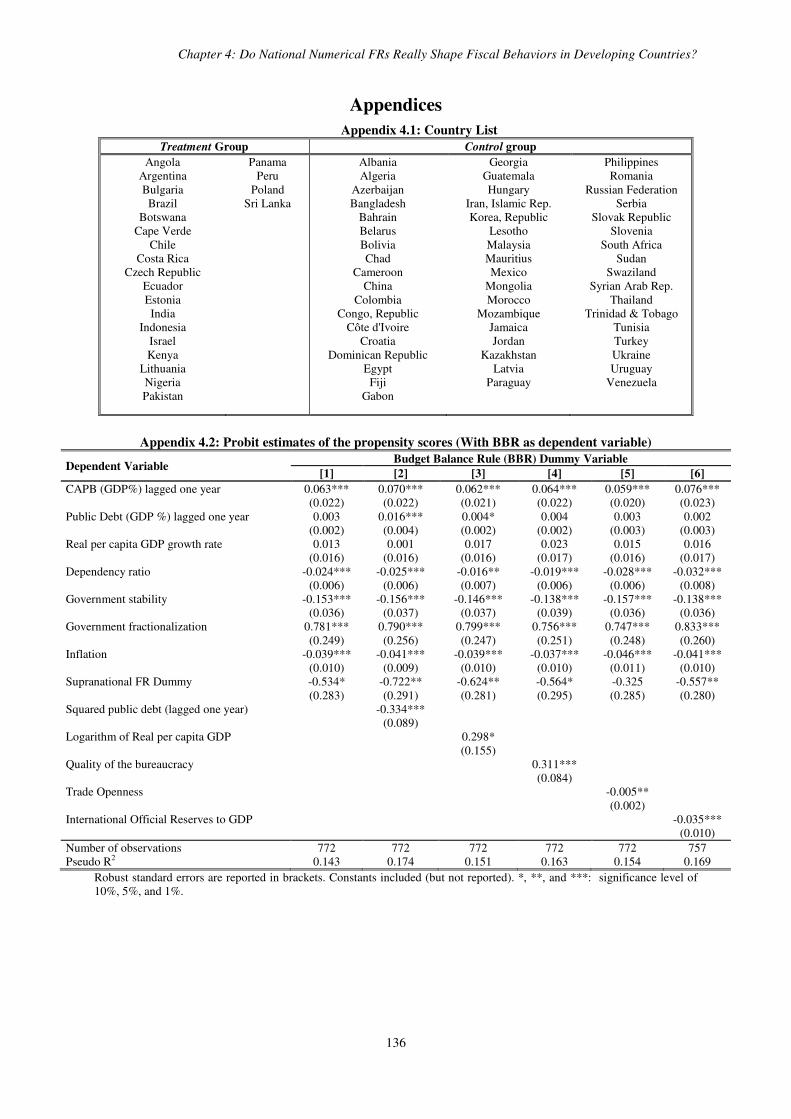
Chapter 4: Do National Numerical FRs Really Shape Fiscal Behaviors in Developing Countries?
136
Appendices
Appendix 4.1: Country List
Treatment Group Control group
Angola Argentina Bulgaria Brazil
Botswana Cape Verde
Chile Costa Rica
Czech Republic Ecuador Estonia India
Indonesia Israel Kenya
Lithuania Nigeria Pakistan
Panama Peru
Poland Sri Lanka
Albania Algeria
Azerbaijan Bangladesh
Bahrain Belarus Bolivia Chad
Cameroon China
Colombia Congo, Republic
Côte d'Ivoire Croatia
Dominican Republic Egypt
Fiji Gabon
Georgia Guatemala Hungary
Iran, Islamic Rep. Korea, Republic
Lesotho Malaysia Mauritius Mexico
Mongolia Morocco
Mozambique Jamaica Jordan
Kazakhstan Latvia
Paraguay
Philippines Romania
Russian Federation Serbia
Slovak Republic Slovenia
South Africa Sudan
Swaziland Syrian Arab Rep.
Thailand Trinidad & Tobago
Tunisia Turkey Ukraine Uruguay
Venezuela
Appendix 4.2: Probit estimates of the propensity scores (With BBR as dependent variable)
Dependent Variable Budget Balance Rule (BBR) Dummy Variable
[1] [2] [3] [4] [5] [6]
CAPB (GDP%) lagged one year 0.063*** 0.070*** 0.062*** 0.064*** 0.059*** 0.076*** (0.022) (0.022) (0.021) (0.022) (0.020) (0.023) Public Debt (GDP %) lagged one year 0.003 0.016*** 0.004* 0.004 0.003 0.002 (0.002) (0.004) (0.002) (0.002) (0.003) (0.003) Real per capita GDP growth rate 0.013 0.001 0.017 0.023 0.015 0.016 (0.016) (0.016) (0.016) (0.017) (0.016) (0.017) Dependency ratio -0.024*** -0.025*** -0.016** -0.019*** -0.028*** -0.032*** (0.006) (0.006) (0.007) (0.006) (0.006) (0.008) Government stability -0.153*** -0.156*** -0.146*** -0.138*** -0.157*** -0.138*** (0.036) (0.037) (0.037) (0.039) (0.036) (0.036) Government fractionalization 0.781*** 0.790*** 0.799*** 0.756*** 0.747*** 0.833*** (0.249) (0.256) (0.247) (0.251) (0.248) (0.260) Inflation -0.039*** -0.041*** -0.039*** -0.037*** -0.046*** -0.041*** (0.010) (0.009) (0.010) (0.010) (0.011) (0.010) Supranational FR Dummy -0.534* -0.722** -0.624** -0.564* -0.325 -0.557** (0.283) (0.291) (0.281) (0.295) (0.285) (0.280) Squared public debt (lagged one year) -0.334*** (0.089) Logarithm of Real per capita GDP 0.298* (0.155) Quality of the bureaucracy 0.311*** (0.084) Trade Openness -0.005** (0.002) International Official Reserves to GDP -0.035*** (0.010) Number of observations 772 772 772 772 772 757 Pseudo R2 0.143 0.174 0.151 0.163 0.154 0.169
Robust standard errors are reported in brackets. Constants included (but not reported). *, **, and ***: significance level of 10%, 5%, and 1%.
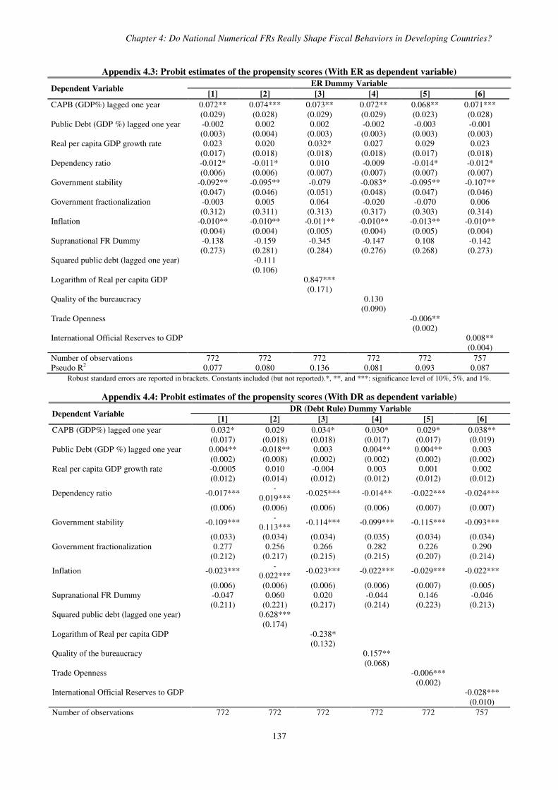
Chapter 4: Do National Numerical FRs Really Shape Fiscal Behaviors in Developing Countries?
137
Appendix 4.3: Probit estimates of the propensity scores (With ER as dependent variable)
Dependent Variable ER Dummy Variable
[1] [2] [3] [4] [5] [6]
CAPB (GDP%) lagged one year 0.072** 0.074*** 0.073** 0.072** 0.068** 0.071*** (0.029) (0.028) (0.029) (0.029) (0.023) (0.028) Public Debt (GDP %) lagged one year -0.002 0.002 0.002 -0.002 -0.003 -0.001 (0.003) (0.004) (0.003) (0.003) (0.003) (0.003) Real per capita GDP growth rate 0.023 0.020 0.032* 0.027 0.029 0.023 (0.017) (0.018) (0.018) (0.018) (0.017) (0.018) Dependency ratio -0.012* -0.011* 0.010 -0.009 -0.014* -0.012* (0.006) (0.006) (0.007) (0.007) (0.007) (0.007) Government stability -0.092** -0.095** -0.079 -0.083* -0.095** -0.107** (0.047) (0.046) (0.051) (0.048) (0.047) (0.046) Government fractionalization -0.003 0.005 0.064 -0.020 -0.070 0.006 (0.312) (0.311) (0.313) (0.317) (0.303) (0.314) Inflation -0.010** -0.010** -0.011** -0.010** -0.013** -0.010** (0.004) (0.004) (0.005) (0.004) (0.005) (0.004) Supranational FR Dummy -0.138 -0.159 -0.345 -0.147 0.108 -0.142 (0.273) (0.281) (0.284) (0.276) (0.268) (0.273) Squared public debt (lagged one year) -0.111 (0.106) Logarithm of Real per capita GDP 0.847*** (0.171) Quality of the bureaucracy 0.130 (0.090) Trade Openness -0.006** (0.002) International Official Reserves to GDP 0.008** (0.004) Number of observations 772 772 772 772 772 757 Pseudo R2 0.077 0.080 0.136 0.081 0.093 0.087
Robust standard errors are reported in brackets. Constants included (but not reported).*, **, and ***: significance level of 10%, 5%, and 1%.
Appendix 4.4: Probit estimates of the propensity scores (With DR as dependent variable)
Dependent Variable DR (Debt Rule) Dummy Variable
[1] [2] [3] [4] [5] [6]
CAPB (GDP%) lagged one year 0.032* 0.029 0.034* 0.030* 0.029* 0.038** (0.017) (0.018) (0.018) (0.017) (0.017) (0.019) Public Debt (GDP %) lagged one year 0.004** -0.018** 0.003 0.004** 0.004** 0.003 (0.002) (0.008) (0.002) (0.002) (0.002) (0.002) Real per capita GDP growth rate -0.0005 0.010 -0.004 0.003 0.001 0.002 (0.012) (0.014) (0.012) (0.012) (0.012) (0.012)
Dependency ratio -0.017*** -
0.019*** -0.025*** -0.014** -0.022*** -0.024***
(0.006) (0.006) (0.006) (0.006) (0.007) (0.007)
Government stability -0.109*** -
0.113*** -0.114*** -0.099*** -0.115*** -0.093***
(0.033) (0.034) (0.034) (0.035) (0.034) (0.034) Government fractionalization 0.277 0.256 0.266 0.282 0.226 0.290 (0.212) (0.217) (0.215) (0.215) (0.207) (0.214)
Inflation -0.023*** -
0.022*** -0.023*** -0.022*** -0.029*** -0.022***
(0.006) (0.006) (0.006) (0.006) (0.007) (0.005) Supranational FR Dummy -0.047 0.060 0.020 -0.044 0.146 -0.046 (0.211) (0.221) (0.217) (0.214) (0.223) (0.213) Squared public debt (lagged one year) 0.628*** (0.174) Logarithm of Real per capita GDP -0.238* (0.132) Quality of the bureaucracy 0.157** (0.068) Trade Openness -0.006*** (0.002) International Official Reserves to GDP -0.028*** (0.010) Number of observations 772 772 772 772 772 757

Chapter 4: Do National Numerical FRs Really Shape Fiscal Behaviors in Developing Countries?
138
Pseudo R2 0.074 0.111 0.079 0.079 0.090 0.094 Robust standard errors are reported in brackets. Constants included (but not reported).*, **, and ***: significance level of 10%, 5%, and 1%.
Appendix 4.5: Heterogeneity in the effect of FR on the CAPB (Country & Time Fixed Effect Estimations)
Dependent Variable: CAPB (GDP %) [1] [2] [3] [4] [5] [6] [7]
FR Dummy 2.660** 2.430** -0.266 2.281** 2.607** 3.041** -1.931 (1.208) (1.133) (2.199) (1.019) (1.134) (1.415) (2.866) Propensity Score 4.513* 4.355* 4.398* 4.660* 5.354* 6.053** (2.302) (2.222) (2.243) (2.817) (2.813) (2.912) FR * Number of FRs 1.671* (0.852) FR * Time 0.0709 (0.279) Supranational Dummy 1.199* (0.612) FR * Supranational -1.875* (0.956) Government Fractionalization -0.730 (0.887) FR *Government Fractionalization -3.893* (1.986) Government stability 0.093 (0.159) FR *Government Stability 0.531* (0.271) Country Fixed Effects Yes Yes Yes Yes Yes Yes Yes Time Fixed Effects Yes Yes Yes Yes Yes Yes Yes Observations 768 768 768 768 768 768 768 R2 0.133 0.141 0.152 0.141 0.145 0.152 0.150
Note: CAPB: Cyclically-Adjusted Primary Balance. In brackets the bootstrapped standard errors (with 500 replications). *, **, and *** indicate the significance level of 10%, 5%, and 1%, respectively. Constant terms are included but not reported.
Appendix 4.6: Heterogeneity in the effect of ER on the CAPE (Country and Time Fixed Effect Estimations)
Dependent Variable: CAPE (GDP %) [1] [2] [3] [4] [5] [6] [7]
ER Dummy -3.048** -2.523* -3.376 -2.470 -2.766* -4.873*** 3.728 (1.456) (1.418) (2.491) (1.748) (1.603) (1.436) (2.706) Propensity Score -21.55*** -21.77*** -21.51*** -21.23** -21.78*** -20.62** (8.240) (8.303) (8.242) (8.258) (8.365) (8.128) ER * Number of FRs 0.486 (1.582) ER * Time -0.015 (0.215) Supranational Dummy 0.642 (0.808) ER * Supranational 1.996* (1.018) Gov. Fractionalization -0.070 (0.826) ER *Gov. Fractionalization 8.986*** (2.263) Government stability 0.209* (0.107) ER *Government Stability -0.751** (0.319) Country Fixed Effects Yes Yes Yes Yes Yes Yes Yes Time Fixed Effects Yes Yes Yes Yes Yes Yes Yes Observations 762 762 762 762 762 762 762 R2 0.127 0.144 0.144 0.144 0.147 0.170 0.152
Note: ER=Expenditure Rule; CAPE=Cyclically-Adjusted Primary Expenditure. In brackets the bootstrapped standard errors (with 500 replications). *, **, and *** indicate the significance level of 10%, 5%, and 1%, respectively. Constant terms are included but not reported.

Chapter 4: Do National Numerical FRs Really Shape Fiscal Behaviors in Developing Countries?
139
Appendix 4.7
4. 9: Structural Primary balance, 1990-2007
0.0
-0.0
-0.8
1.0
-1-.5
0.5
1
Structu
ral prim
ary
bala
nce (G
DP
%)
FR_non-treated FR_treated
Pre-FR period Post-FR period
4. 10: Structural primary expenditure, 1990-2007
-0.9
0.20.2
-0.4
-1-.
50
.5
Structu
ral prim
ary
Expenditure
(G
DP
%)
FR_non-treated FR_treated
Pre-FR period Post-FR period
4. 11: Gross Public Debt, 1990-2007
77.9
67.7 68.1
42.9
020
40
60
80
Gro
ss P
ublic
Debt (G
DP
%)
FR_non-treated FR_treated
Pre-FR period Post-FR period
Notes for Figures 4.1, 4.2 and 4.3: FR_treated Vs. FR_non-treated Sources: World Economic Outlook, WEO (2011) for Figures 4.1 and 4.2; Ali Abbas et al. (2010) for Figure 4.3.

Chapter 4: Do National Numerical FRs Really Shape Fiscal Behaviors in Developing Countries?
140
Appendix 4.8: Descriptive Statistics
Variable Obs Mean Std. Dev. Min Max
Cyclically-Adjusted Primary Fiscal Balance (GDP %) 1074 0.016 3.492 -18.344 24.618 Cyclically-Adjusted Primary Expenditure (GDP %) 1075 -0.188 3.660 -26.182 25.411 Government Debt (GDP %) 1195 56.838 41.593 3.742 454.864 Fiscal Rule (FR) 1332 0.131 0.337 0.000 1.000 Budget Balance Rule (BBR) 1332 0.092 0.289 0.000 1.000 Expenditure Rule (ER) 1332 0.035 0.185 0.000 1.000 Revenue Rule (RR) 1332 0.013 0.112 0.000 1.000 Debt Rule (DR) 1332 0.068 0.251 0.000 1.000 Supranational Dummy 1314 0.066 0.249 0.000 1.000 Real per capita GDP growth rate 1280 2.670 5.803 -32.935 44.281 Dependency ratio 1332 64.997 16.581 38.100 106.900 Government stability 1118 8.008 2.003 1.000 12.000 Government Fractionalization 1197 0.224 0.273 0.000 0.893 Inflation 1279 55.109 340.794 -11.686 7481.664 Number of FR 1332 0.191 0.543 0.000 3.000 Time since FR adoption 1332 0.748 2.894 0.000 28.000 Real per capita GDP 1292 7223.490 4777.399 955.786 26306.430 Quality of the bureaucracy 1118 2.023 0.845 0 4 Trade Openness 1292 80.787 41.214 10.094 222.288 International Official Reserves to GDP 1254 15.047 14.009 0 114.448
Appendix 4.9: Sources and definitions of data
Variables Definition Sources
Fiscal Rule (FR) Dummy Variable taking the value 1 if in a given year a country has in place, a
national numerical constraint on government budget aggregates.
Fiscal Rules Database by the IMF’s Fiscal Affairs
Department, Fiscal Policy and Surveillance Division (2009),
available at www.imf.org/external/np/ pp/eng/2009/121609.pdf
Budget Balance Rule (BBR)
Expenditure Rule (ER)
Revenue Rule (RR)
Debt Rule (DR)
Supranational Dummy
Dummy Variable taking the value 1 if in a given year a country has in place, a national numerical constraint on government Fiscal Balance.
Dummy Variable taking the value 1 if in a given year a country has in place, a national numerical constraint on government Expenditure.
Dummy Variable taking the value 1 if in a given year a country has in place, a national numerical constraint on government Revenue.
Dummy Variable taking the value 1 if in a given year a country has in place, a national numerical constraint on government Debt.
Dummy Variable taking the value 1 if in a given year a country has in place, a supranational numerical constraint on government fiscal aggregates.
Structural Primary Fiscal Balance
Structural Primary Expenditure
Difference between General Government revenue and expenditure (excluding interest payments), adjusted for business fluctuations, as GDP percentage. General government expenditure excluding interest payments, adjusted for
business fluctuations, as GDP percentage.
Author’s calculations based on
World Economic Outlook (WEO, 2010)
Government Debt Gross General government debt, as GDP percentage Ali Abbas et al. (2010) Real per capita GDP growth rate Annual growth rate of real output per capita
Penn World Table (PWT6.3) Trade openness Sum of imports and exports divided by GDP Real per capita GDP GDP per capita at constant prices.
Inflation
Annual growth rate of average CPI World Economic Outlook
(WEO, 2010)
Government stability
Index ranging from 0 to 12 and measuring the ability of government to stay in office and to carry out its declared program(s).The higher the index, the more
stable the government is. International Country Risk
Guide (ICRG, 2009)
Quality of the bureaucracy Index ranging from 0 to 4 and measuring the institutional strength and
expertise that the bureaucracy has to govern without drastic changes in policy or interruptions in government services.
Government Fractionalization Index measuring the Probability that two deputies picked at random among
from the government parties will be of different parties. World Bank Database of
Political Institutions (2010)
Dependency Ratio Ratio of dependents (people younger than 15 or older than 64) to working-age
population (those ages 15-64) World Development Indicators
(WDI, 2010) Total Official reserves
Total reserves comprise holdings of monetary gold, special drawing rights, reserves of IMF members held by the IMF, and holdings of foreign exchange
under the control of monetary authorities.

Chapter 4: Do National Numerical FRs Really Shape Fiscal Behaviors in Developing Countries?
141
Appendix 4.10: Strength of the instruments in the 2SLS estimations of the CAPB (key test statistics)
Country 1st step F-Statistic
Shea's Partial R2 Country 1st step F-Statistic Shea's Partial R2
Albania 4,026 20,609 Jamaica 16,110 38,874 Algeria 13,495 40,149 Jordan 7,185 96,424 Angola 29,271 66,217 Kazakhstan 6,949 78,133
Argentina 19,860 39,684 Kenya 30,856 55,671 Azerbaijan 15,210 47,783 Korea, South 4,845 20,089
Bahrain 12,149 12,679 Latvia 54,175 85,632 Bangladesh 17,237 33,684 Lesotho 8,621 20,203
Belarus 14,547 68,915 Lithuania 15,126 39,706 Bolivia 38,734 58,501 Malaysia 25,590 42,945
Botswana 34,775 58,553 Mauritius 16,772 34,126 Brazil 14,882 32,015 Mexico 14,064 23,990
Bulgaria 30,449 68,911 Mongolia 21,202 51,623 Cameroon 67,185 73,437 Morocco 5,481 8,164
Cape Verde 5,934 2,560 Mozambique 5,291 8,672 Chad 13,706 27,429 Nigeria 19,133 34,812 Chile 11,241 24,787 Pakistan 24,702 27,497 China 29,767 87,034 Panama 14,167 32,855
Colombia 46,529 58,981 Paraguay 4,440 88,059 Congo 18,401 1,795 Peru 25,213 59,021
Costa Rica 12,219 49,645 Philippines 4,010 29,161 Cote d'Ivoire 38,633 53,911 Poland 6,978 29,281
Croatia 42,304 82,674 Romania 6,466 20,803 Czech Republic 14,792 62,529 Russia 33,342 41,799
Dominican Republic 14,208 48,548 Serbia 4,305 14,683 Ecuador 10,121 53,928 Slovakia 12,194 55,197 Egypt 16,883 28,922 South Africa 25,328 69,019
El Salvador 15,579 49,139 Sri Lanka 23,466 44,097 Estonia 18,083 74,633 Sudan 6,305 12,588
Fiji 4,012 2,602 Swaziland 14,378 29,410 Gabon 6,688 9,525 Syria 4,977 10,862
Georgia 8,767 41,462 Thailand 17,639 40,194 Guatemala 7,506 25,355 Trinidad & Tobago 6,130 35,457 Hungary 85,210 45,385 Tunisia 6,358 3,690
India 20,087 51,373 Turkey 7,325 23,807 Indonesia 338,076 98,888 Ukraine 97,600 98,079
Iran 17,732 41,941 Uruguay 23,414 47,324 Israel 4,005 53,022 Venezuela 10,001 35,960

142

143
Chapter 5
Does Inflation Targeting
Improve Fiscal Discipline?
“Inflation Targeting […] compels policymakers to deepen reforms, enhance transparency, and improve the fiscal stance”
(E. Croce & M. Khan, Finance and Development, September 2000, Volume 37, Number 3, p.51)

Chapter 5: Does IT Improve Fiscal Discipline?
144
5.1. Introduction
The present chapter of the dissertation extends the literature on the macroeconomic
consequences of IT by focusing on the linkage between IT monetary regimes and fiscal
policy. In addition to the monetarist view, which defends an exclusive role for monetary
policy regarding inflation dynamics, an influential strand of the literature, inspired by the
seminal contribution of Sargent & Wallace (1981), points out that fiscal policy can equally be
a source of inflation (see, e.g., Aiyagari & Gertler, 1985; Sims, 1988; or Leeper, 1991, for a
discussion on price level determinacy, and Woodford’s, 1994, fiscal theory of price level).
Indeed, in a context of fiscal dominance (i.e. when fiscal balances evolve independently of
public debt so that the equilibrium price level changes to ensure fiscal solvency), a restrictive
monetary policy may even result in higher inflation if the main source of government funding
is seigniorage, and if the fiscal balance is not adjusted after seigniorage receipts collapse (such
a reasoning appears in Sims, 2011, who analyses the role of fiscal policy in the inflation of the
1970s).
These findings influenced the implementation of IT regimes. Indeed, in addition to
conventional monetary preconditions (a sufficient degree of central bank operational
independence, a sound financial system, a resilience to changes in exchange and interest rates,
absence of dollarization, absence of price regulation, and the availability of a developed
technical infrastructure for forecasting the inflation process and the transmission mechanism,
see Amato & Gerlach, 2002; or Batini & Laxton, 2007), several authors, including Masson et
al. (1997), Mishkin (2000), Sims (2004), or Bernanke & Woodford (2004), have expressed
doubts on the feasibility of IT in the presence of fiscal dominance and/or a poor fiscal stance,
and consequently suggested extending preconditions for IT adoption to sustainable fiscal
policies.
However, contrary to the undeniable role of fiscal discipline (FD) as a prerequisite for IT
implementation, little is said about the eventual effect of IT adoption on FD. The aim of the
present chapter is to investigate precisely this possible reversed effect, i.e. could the adoption
of IT lead to the improvement of the fiscal stance? This is all the more plausible since, as
pointed out by Amato & Gerlach (2002) and Batini & Laxton (2007), most IT countries, and
especially developing countries, did not satisfy the prerequisites for a credible IT adoption,
including in terms of FD. Accordingly, to convince private agents and financial markets that

Chapter 5: Does IT Improve Fiscal Discipline?
145
such bad fiscal stance prior to IT adoption will not be an impediment toward hitting the
inflation target, a discipline-enhancing effect on the conduct of fiscal policy may have
followed IT adoption in these countries. Consequently, even though IT is not directly devoted
to fiscal goals, the fear of missing the inflation target may however be sufficiently binding for
monetary, as well as for fiscal authorities, so that it will have a side effect on FD.102 This
stems from the fact that a credible adoption of IT requires the joint commitment of the central
bank and the government in hitting the inflation target.103 Moreover, good theoretical
arguments suggest that, even if IT is primarily devoted to inflation goals, IT adoption could
also lead to a FD improvement. We discuss these arguments with respect to two of the most
important features of IT regimes, namely (i) credibility and (ii) commitment to a low (single
digit) inflation target.
On the one hand, Roger (2009) and Freedman & Ötker-Robe (2010) stressed out that IT
adoption may catalyze the implementation of FD for preserving the viability of the IT regime
itself (a direct argument).104 For example, according to Mishkin (2000), fiscal policy should
be kept sound enough to eliminate any speculation regarding a possible monetization of
public debt in the future, which would have dramatic consequences on the merely existence of
the IT monetary regime.
On the other hand, the fact that IT regimes lead to low inflation rates (see, e.g., Vega &
Winkelried, 2005; Pétursson, 2005; Batini & Laxton, 2007; Mishkin & Schmidt-Hebbel,
2007; Gonçalves & Salles, 2008; or Lin & Ye, 2009) has multiple consequences on the way
the government conducts fiscal policy (indirect, inflation-based, arguments). First, in light of
the Tinbergen’s rule, and given the overriding goal of price stability assigned to MP under IT,
interest rates can no longer be used to achieve both price stability and fiscal solvency.
Consequently, this is likely to leave the government with the improvement of FD as the only
102 For example, IT may act as a “tying your own hands” mechanism and rule out the so-called “deficit bias” (Buchanan & Wagner, 1977; Kydland & Prescott, 1977; and Cukierman & Meltzer, 1986), by preventing fiscal authorities from manipulating fiscal policy for electoral purposes. 103 This is why IT implementation goes along with the adoption of legislation measures prohibiting monetization of public debt, while in some countries the inflation target is jointly defined by the central bank and the government, in order to send a clear signal about their joint willingness to respect the inflation target (see Freedman & Ötker-Robe, 2010). 104 The fact that IT may fail in anchoring credibly inflation expectations in a country with bad fiscal stance is well documented in the literature (see, e.g., Loyo, 1999; Sims, 2004; Bernanke & Woodford; 2004, Favero & Giavazzi, 2005; or Blanchard, 2005).

Chapter 5: Does IT Improve Fiscal Discipline?
146
main instrument to meet its intertemporal budget constraint.105 Second, lower inflation rates
weaken seigniorage revenue, a loss which can be compensated by either alternative financing
sources (mainly taxes, since the public debt must be kept under strict control), or a better
collection of resources, through a strengthening of the tax collection system.106 Altogether,
these arguments could support a possible increase in FD following the adoption of an IT
monetary regime.
To explore the possible existence of an effect from IT to FD, we follow the very recent
contributions of Vega & Winkelried (2005) and Lin & Ye (2007, 2009), and draw upon a
variety of propensity scores-matching methods. Evidence based on a sample of both
developing and developed countries shows that IT exerts a positive and significant effect on
FD. To the best of our knowledge, this is the first study emphasizing such an effect running
from IT towards FD. Besides, our result is found to be extremely robust when (i) using
different measures of FD, (ii) considering alternative specifications for computing propensity
scores, or (iii) when accounting for different definitions of IT starting dates (i.e. conservative
or default dates).
Moreover, we extend our analysis by studying the relation between IT and FD on the group of
developed, respectively developing countries. Although IT does not seem to exert a robust
effect on FD in developed countries (the ATT is positive but not statistically significant), we
show that developing countries significantly improved their FD following the adoption of an
IT monetary regime. A possible explanation is that developed countries were judged by
financial markets as presenting sustainable fiscal stance when they adopted IT, so their efforts
to increase FD following IT adoption is not significant, while developing countries adopted IT
despite the presence of potential risks on their fiscal stance, but were forced to improve their
FD following IT adoption to maintain the durability of the IT regime.
105 The same holds regarding the effect of IT on FD via the exchange rate channel. Since in an IT regime central banks should react to exchange rate movements only when they affect inflation, IT adoption should go hand in hand with more de facto flexible exchange rates (Roger, 2009), and, according to Tornell & Velasco (2000), with more FD. 106 This strengthening of the tax collection system is all the more welcomed under an IT regime, since low inflation rates mitigate the negative Oliveira-Keynes-Tanzi effect (the erosion in the real value of taxes between the date of imposition and the date of collection decreases, see Tanzi, 1992), while the decrease in inflation volatility (outlined, among others, by Mishkin & Schmidt-Hebbel, 2007; Gonçalves & Salles, 2008; or Lin & Ye, 2009) allows stabilizing and making more predictable the tax base, improving therefore tax collection.

Chapter 5: Does IT Improve Fiscal Discipline?
147
To sum up, our results have policy implications that could contribute to the current debate
regarding the relevance of IT adoption in general, and particularly for developing countries.
Indeed, whilst most existing studies simply point out that FD is a prerequisite for a credible
adoption of IT, our findings, in addition to not denying this reality, go beyond it and suggest
that IT adoption could enhance FD, especially in developing countries. Consequently, IT
adoption, by improving FD, can maintain or strengthen macroeconomic stability, which is a
key factor in the strength of a country’s financial system, and hence a precondition for a
strong and balanced long term economic growth (Fischer, 1993). Indeed, in the current
context of financially integrated markets, weak FD and weak banking system may feed
negatively on each other to compromise stability and growth, and even lead to economic and
financial crises (Mishkin, 1996). Maintaining FD is also important in that it allows reducing
the vulnerability of a country to interest rate and economic growth shocks. In addition, recent
contributions (including Minea & Villieu, 2009; Kumar & Woo, 2010; Reinhart & Rogoff,
2010; or IMF, 2011d), emphasized that debt levels beyond certain thresholds may reduce
economic growth, which itself might fuel the debt distress problem. Finally, sound fiscal
policies may provide room for policymakers to foster economic growth through the provision
of public goods (particularly physical and social infrastructures), and to conduct
countercyclical fiscal policies to buffer the adverse effects of unexpected shocks (Chalk &
Hemming, 1998).
The rest of the chapter is organized as follows. Section two briefly displays some stylized
facts. Section three presents the dataset and discusses the methodology, section four shows
the matching results, and then illustrates the influence of IT adoption on FD for the full
sample and for developed and developing countries respectively, and section five concludes.
5.2. Stylized facts
Before introducing the dataset and describing the econometric methodology, let observe some
stylized facts relating IT to primary aspects of FD, namely the Debt-to-GDP ratio as well as
its relative change.
The left-hand chart of Figure 5.1 shows that the average public debt (in % of GDP) is lower
in the ITers, compared to the non-ITers. But this naive correlation cannot be evidence of

Chapter 5: Does IT Improve Fiscal Discipline?
148
better FD recorded by the ITers, as it may only reflect a “self-selection” result, i.e. countries
with lower public debt are those that more likely adopt IT. To mitigate this self-selection
problem in IT adoption, we present in the right-hand chart of Figure 5.1 the evolution of debt-
to-GDP ratio for the ITers and the non-ITers, respectively. If we take as reference the middle
year before the first IT adoption (1990, New Zealand) and the last IT adoption (2002, Peru
and Philippines) for the countries in our sample, namely 1996, we can see that, although on
average both ITers and non-ITers presented downward trends in their debt ratios before 1996,
only ITers managed to maintain this decrease in the years just after 1996.
Figure 5. 1: Public debt (in % of GDP) in IT compared to non-IT countries
46.6
56.5
0
20
40
60
ITers Non ITers
30
40
50
60
70
1985 1990 1995 2000 2005 2010
ITers Non ITers
Note for Figures 1 and 2: data on public debt come from the recent database of Ali Abbas et al. (2010).
Of course, this interpretation may be criticized on the basis that it compares public debt
evolution before and after a common year (1996) for IT adoption for all countries in the
sample. Figure 5.2 below illustrates one way to avoid this problem, by presenting statistics at
country-level. For generality, we display countries having adopted IT at the beginning of our
sample (namely, New Zealand, 1990, and Sweden, 1995) and at the end of our sample
(namely, Mexico, 2001, and Peru, 2002). For each of these countries, we present the change
in the debt-to-GDP ratio between the year of IT adoption and the last year of our sample
(2007), as well as the change in the debt-to-GDP ratio between the same period for countries
that have not adopted IT, but display relatively close debt-to-GDP ratios in the year of IT
adoption of the ITers. As depicted by Figure 5.2, the debt ratio decreased in the ITers, while it
increased (or at best changed marginally) in the non-ITers, during the same time period, and
controlling for the fact that these countries presented relatively close debt ratios in the year of
IT adoption. Consequently, Figure 5.2 shows the existence of large discrepancies regarding
the evolution of the debt ratio in ITers compared to non-ITers (the relative difference between
the two categories of countries is presented in brackets, and is measured in percentage point
changes). This therefore provides a first indication that IT adoption seems to improve FD.

Chapter 5: Does IT Improve Fiscal Discipline?
149
But, is such a correlation corroborated by a more rigorous econometric analysis? Next
sections of this chapter will focus on addressing this issue.
Figure 5. 2: The change in the debt-to-GDP ratio: ITers vs. non ITers
61.7
55.3 56.2
17.4
62.159.2
0
20
40
60
80
New Zealand (1990) USA Austria
1990 (IT starting date) 2007 (end of sample)
81.092.4
99.2
40.1
187.7
95.6
0
40
80
120
160
200
Sweden (1995) Japan Greece
1995 (IT starting date) 2007 (end of sample)
44.340.6
45.6
38.2
63.0
49.0
0
20
40
60
80
Mexico (2001) Uruguay Mauritius
2001 (IT starting date) 2007 (end of sample)
40.343.1
46.0
30.9
42.7
47.3
0
20
40
60
Peru (2002) Malaysia Fiji
2002 (IT starting date) 2007 (end of sample)
5.3. Dataset and methodology
5.3.1. Dataset
Our dataset consists of 84 countries, of which 62 developing and 22 developed countries,
examined over the 1985-2007 period. Among the 84 countries, 28 countries (called ITers or
treatment group) adopted IT by the end of 2007. Due to lack of data on FD, Romania and
Serbia, which adopted IT in 2005 and 2006 respectively, do not appear in our sample.
Moreover, given that our sample ends up in 2007, we still treat the new ITers as non ITers.107
Accordingly, this leaves us with 23 ITers. In addition, to ensure that non-ITers (called control
group) are a good counterfactual of the treatment group, i.e. the two groups are reasonably
comparable, we follow Lin & Ye (2009) and include in the control group only non-ITers that
have a real per capita GDP at least as large as that of the poorest ITer, and with a population
107 New ITers are countries having adopted IT after 2005, namely Indonesia (2005), Slovak Republic (2005), Guatemala (2005), Turkey (2006) and Ghana (2007).
-71.8%
-13.8%
-23.3%
+55.0%
+7.6%
-0.80% [-22.5pp]
+2.8%
+12.5% [-84.2pp]
+5.4%
[-77.2pp] -50.6%
+103.0% [-153.6pp]
-3.7%

Chapter 5: Does IT Improve Fiscal Discipline?
150
size at least as large as that of the smallest ITer.108 The 23 ITers and the 61 control countries
that satisfy these criteria are listed in Appendices 5.1 and 5.2 respectively.109
Data on starting dates of IT come from Rose (2007), who distinguishes two dates, namely
default starting years and conservative starting years (see Appendix 5.1).110 For robustness
issues, we perform our analysis on both dates.
Let us now discuss in detail our outcome variable, namely FD. Remark that despite the
relative consensus among macroeconomists and policymakers regarding the crucial
importance of FD in preserving macroeconomic stability, reducing vulnerabilities, and
improving aggregate economic performance, there is no accurate definition of the concept of
FD. Most of the time, FD is commonly associated with the notions of fiscal policy
sustainability and public debt sustainability, which are two inter-related concepts whose
analysis is a complex and multifaceted exercise. Both concepts are supposed to reflect at best
the government’s fiscal stance, and a simple rule of thumb that generally emerges from their
analysis is that a government’s fiscal policy will be regarded as disciplined if its fiscal policy,
as well as its public debt, is sustainable (IMF, 2011d). First, public debt sustainability relates
to the government long-term solvency: assuming that the interest rate on public debt exceeds
the growth rate of the economy, the government’s public debt will be said sustainable when
its intertemporal budget constraint is met, namely when its debt-to-GDP ratio is stable
(Bartolini & Cottarelli, 1994). Second, fiscal policy sustainability relates to the liquidity of the
government’s short-term assets, namely its ability to run primary fiscal balance capable of
stabilizing the debt-to-GDP ratio without resorting to a fiscal adjustment and/or a debt
restructuring.111
From an operational viewpoint, as underlined by Tornell & Velasco (2000), FD is defined and
measured in terms of meeting some numerical thresholds on key fiscal aggregates, namely the
108 The poorest ITer in our sample is Philippines with a real per capita GDP of 3994 USD in 2004 (the year just before the starting date of the new ITers), while the smallest ITer in terms of population size is Iceland, with around 0.3 million inhabitants in 2004. 109 Finally, note that Finland and Spain, which adopted IT respectively in 1993 and 1995, abandoned it in 1999 to join the Euro area. We therefore treat them as ITers between 1993-1998 and 1995-1998, respectively, and as non-ITers after 1999. 110 See chapter 1, section 1.2.1 for further details on the differences between these two kinds of date. 111 It is worth noting that a government’s fiscal policy may be currently unsustainable, whereas its public debt can be regarded as sustainable. Indeed, the current level of the primary balance might not be sufficient to stabilize the debt-to-GDP ratio, but a sufficient fiscal adjustment would be realistic (both economically and politically) to bring the primary balance to a level that is necessary to service public debt.

Chapter 5: Does IT Improve Fiscal Discipline?
151
fiscal balance and the debt-to-GDP ratio.112 However, as emphasized by IMF (2011d), these
thresholds should be employed flexibly to trigger in-depth analysis of the fiscal risks and
fiscal vulnerabilities faced by a country, once its fiscal performances breach them, rather than
considered as actual systematic indicators of FD. When it comes to performing econometric
analysis regarding the FD, Bénassy-Quéré & Pisani-Ferry (1994) suggest measuring it with
indicators derived from the accounting relationships between public debt and fiscal balances,
namely the annual change in the fiscal balance (overall balance and/or primary balance) and
the annual change in the debt-to-GDP ratio.
Nevertheless, the relevance of these indicators as actual measures of FD is subject to debate.
As acknowledged in the literature (see, e.g., Gali & Perotti, 2003; Fatás & Mihov, 2003; or,
more recently, Debrun et al., 2007a), fiscal balances are the result of fiscal decisions of
policymakers (structural component) and the effects of business cycle fluctuations (cyclical
component). Since the latter is not under the direct control of the government (at least in the
short term), it is important to filter out the impact of business cycle fluctuations (automatic
stabilizers) on the primary and/or overall fiscal balance, to better capture fiscal behavior.
Accordingly, we measure FD by the (i) Cyclically-Adjusted Primary Fiscal Balance (CAPB)
and the (ii) Cyclically-Adjusted overall Fiscal Balance (CAB) respectively, both as
percentage of GDP.113 In addition, for the sake of further robustness check, we also employ
the (iii) relative change in the debt-to-GDP ratio as a subsequent alternative measure of FD
(consistently with the stylized facts exposed in section 5.2). Appendices 5.3 and 5.4 present
the definitions, sources and descriptive statistics of all variables used in our analysis.
5.3.2. Methodology
We aim at evaluating the treatment effect of IT adoption on FD114 in countries having adopted
IT (ITers), namely the so-called average treatment effect on the treated (ATT)
( )[ ] [ ] [ ]111 0101 =−===−= iiiiiii ITFDEITFDEITFDFDEATT , (5.1) 112 Such measures of FD appear in some monetary unions, as for example the EMU or the WAEMU. In the former case, FD is regarded as the ability of a government to maintain a fiscal balance (as percentage of GDP) and a debt-to-GDP ratio lower than 3% and 60% respectively, while in the latter these thresholds are set to 0% (for the basic balance) and 70% respectively. 113 Appendix 5.5 reveals the calculation of these two variables. 114 Recall that we measure FD in three alternative ways, namely the Cyclically-Adjusted Primary fiscal Balance (CAPB), the Cyclically-Adjusted overall fiscal Balance (CAB) and the relative change in the debt-to-GDP ratio.

Chapter 5: Does IT Improve Fiscal Discipline?
152
where iIT is a dummy variable, which equals 1 if the country i is targeting inflation and 0 if
not. 11 =ii ITFD measures the change in FD if country i has adopted IT, and 10 =ii ITFD
measures the change in FD that would have been observed if the country i had not adopted
IT. Equation (5.1) therefore compares the outcome value, namely FD, observed in the
treatment group (ITers), with the outcome value that would have been observed in the same
countries if they had not adopted IT. Unfortunately, it is not possible to observe this latter
value, and we face here, as it is common in non-experimental studies, an identification
problem. A conventional approach to circumvent this difficulty is to compare the mean of the
variable FD for the treatment group (ITers), with its mean for the control group (non-ITers).
However, this solution holds provided that the assignment to the treatment is random; yet, IT
adoption may be non-random, since it may be correlated with a set of observable variables
that also affects the outcome variable (FD in our case), leading to the so-called “self-
selection” problem.115 Consequently, a simple comparison of the sample mean value of FD
between the two groups would produce biased estimates of the ATT. To overcome this
selection on observables problem, we make use of a variety of propensity score-matching
methods recently employed in the related treatment literature (see, e.g. Vega & Winkelried,
2005; Lin & Ye, 2007, 2009; Lin, 2010; or Flood & Rose, 2010).
The consistency of the ATT estimate strongly depends on the relevance of the counterfactual
(control or comparison) group. The propensity score-matching methods allow us to pair ITers
with non-ITers that have similar observed characteristics, so that the difference between FD in
ITers and FD in a matched counterfactual is attributable to the treatment, namely the IT
adoption. The technique consists of mimicking a randomized experiment on the basis of
observable characteristics ( X ), namely countries with the same observable characteristics
face a randomized experiment, as to whether they adopt IT or not. The key assumption
underlying this matching method is the conditional independence assumption, namely
XITFD ⊥0 and XITFD ⊥1 , which requires for, conditional on observables X , the
outcomes 0FD and 1FD to be independent of the treatment variable. Under this assumption,
equation (5.1) can be rewritten as
115 See Heckman et al. (1998) and Dehejia & Wahba (2002). Also, note that the selectivity problem here is neither selection on unobservables (omitted variables), nor a Heckman-type sample selection problem (since matching on the propensity scores implicitly assumes that unobservables play no role in the treatment assignment).

Chapter 5: Does IT Improve Fiscal Discipline?
153
[ ] [ ]iiiiii XITFDEXITFDEATT ,0,1 01 =−== , (5.2)
where we replaced [ ]iii XITFDE ,10 = by [ ]iii XITFDE ,00 = , which is observable. However,
as the number of explanatory variables ( X ) increases, such a matching on X would be
difficult to implement in practice. To overcome this high dimension problem, Rosenbaum &
Rubin (1983) suggest carrying out the matching using propensity scores, instead of X , with
the propensity score defined as the probability of adopting the IT regime conditional on the
observable variables X , namely ( ) [ ] ( )iiiii XITXITEXp 1Pr === . Under the additional
“common support” assumption (namely, ( ) 1<iXp ), requiring the existence of some
comparable control units (non-ITers) for each treated unit (ITer), the ATT can be estimated as
( )[ ] ( )[ ]iiiiii XpITFDEXpITFDEATT ,0,1 01 =−== . (5.3)
We consider four commonly used propensity score-matching methods. First, the nearest-
neighbor matching with replacement, which matches each treated unit to the n control units
having the closest propensity scores (we consider 1=n , 2=n and 3=n ). Second we draw
on radius matching, which matches a treated unit to the control units with estimated
propensity scores falling within a radius (or caliper) of length r (we consider a large radius
10.0=r , a medium radius 05.0=r , and a small radius 01.0=r ).116 The third method is the
regression-adjusted local linear matching developed by Heckman et al. (1998). Finally, we
employ (Epanechnikov) kernel matching, which matches a treated unit (an ITer) to all control
units (non-ITers) weighted proportionately by their closeness (in terms of propensity scores)
to the treated unit. Since the matching estimator has no analytical variance, we follow Dehejia
& Wahba (2002) and compute standard errors by bootstrapping (i.e. by re-sampling the
observations of the control group).
116 As in Lin (2010), the medium radius is set equal to the standard deviation of the estimated propensity scores while the large and the small radius are set equal to the double and the half of the medium radius, respectively.

Chapter 5: Does IT Improve Fiscal Discipline?
154
5.4. The influence of IT adoption on Fiscal Discipline (FD)
5.4.1. The estimation of propensity scores
We estimate the propensity scores using a probit model,117 in which the dependent variable is
a binary variable, taking the value 1 if in a given year a country operates under IT framework
and zero if not. We consider two sets of explanatory variables, namely one to account for the
fact that a country should reasonably adopt IT after having met some preconditions, and the
other to account for the likelihood for a country to adopt an alternative framework for MP (for
example, exchange rate or money growth targeting).
The precondition variables include lagged inflation rate, central bank governors’ turnover
rates (reverse proxy for independence of the central bank), lagged debt-to-GDP ratio, real per
capita GDP growth rate and CAPB (or alternatively CAB or the change in the debt-to-GDP
ratio). We expect a negative correlation between the probability of IT adoption and the first
three variables and a positive correlation with the last two variables (except for the coefficient
of the change in the debt-to-GDP ratio which is expected to be negative). Concerning the
second set of controls, we consider a fixed exchange rate regime dummy and trade openness.
We expect a negative correlation between the probability of IT adoption and these two
variables.118
Before going any further, let us point out that past FD is included in the probit model in order
to control for the fact that even though IT can improve FD (as we intend to show in this
study), initial (past) fiscal stances could also be a determinant of IT adoption. Indeed, on the
one hand, better fiscal balance (CAPB or CAB), or a past reduction in the debt-to-GDP ratio,
may influence positively the probability of IT adoption. On the other hand, past fiscal
performances can also affect current fiscal outcomes. First, poor past FD may be associated
with high interests on the issued debt, which worsens current FD. Second, poor past FD can
stimulate the government to proceed to adjustments for ensuring solvency, which improves
current FD. Consequently, past fiscal aggregates, as measured by lagged CAPB, lagged CAB
or lagged change in the debt-to-GDP ratio, may affect IT adoption as well as current FD, and
117 Using a Logit model does not change the results. 118 It is important to keep in mind that, when estimating propensity scores, the goal is not to find the best statistical model to explain the probability of IT adoption; according to the conditional independence assumption, omitting in the probit regression variables that systematically affect the targeting probability, but do not affect FD, has little influence on results (Persson, 2001).

Chapter 5: Does IT Improve Fiscal Discipline?
155
their inclusion in the probit model allows ruling out to some extent any polluting effect
arising from a likely two-way relationship between IT and FD.
Table 5. 1: Probit estimates of the Propensity Scores (Full Sample)
Dependent variable : Inflation Targeting (Conservative starting dates)
[1] [2] [3] [4] [5] [6] [7]a
Inflation (lagged one year) -0.102*** -0.102*** -0.101*** -0.102*** -0.102*** -0.083*** -0.102*** (0.011) (0.011) (0.011) (0.013) (0.011) (0.011) (0.011) Governors’ turnover rate -0.844** -0.847** -0.918*** -0.842** -0.857** -0.856** -0.838** (0.363) (0.359) (0.349) (0.366) (0.358) (0.383) (0.364) Debt/GDP (lagged one year) -0.007*** -0.007*** -0.006*** -0.007*** -0.006*** -0.009*** -0.007*** (0.002) (0.002) (0.002) (0.002) (0.002) (0.002) (0.002) Real per capita GDP growth rate 0.016 0.015 0.002 0.016 0.012 0.015 0.016 (0.015) (0.014) (0.014) (0.015) (0.015) (0.015) (0.015) Fixed Exchange rate dummy -1.450*** -1.456*** -1.374*** -1.449*** -1.408*** -1.404*** -1.450*** (0.128) (0.126) (0.122) (0.133) (0.133) (0.129) (0.128) Trade Openness -0.005*** -0.005*** -0.004*** -0.005*** -0.005*** -0.003*** -0.005*** (0.001) (0.001) (0.001) (0.001) (0.001) (0.001) (0.001) CAPB (lagged one year) 0.024 0.024 0.028 0.006 0.024 (0.021) (0.021) (0.020) (0.021) (0.021) CAB (lagged one year) 0.016 (0.020) Debt Change (lagged one year) -0.351 (0.303) Log of real per capita GDP 0.004 (0.101) Domestic credit to private sector -9.42e-07 (2.17e-06) Fiscal rule dummy 0.625*** (0.148) Constant 1.116*** 1.133*** 0.912*** 1.073 1.101*** 0.719*** 1.113*** (0.184) (0.181) (0.168) (1.065) (0.188) (0.194) (0.185) Number of observations 982 1030 1140 982 923 982 914 Pseudo R2 0.341 0.347 0.325 0.341 0.341 0.365 0.323
a Excluding hyperinflation episodes. Robust standard errors in brackets. *, **, and *** indicate the significance level of 10%, 5%, and 1%. CAPB and CAB refer to the Cyclically-Adjusted Primary, and respectively overall, fiscal Balance, both as GDP percentage.
Table 5.1 above reports the probit estimates of propensity scores on the full sample, which
includes both developing and developed countries, based on conservative starting dates of
IT.119 As expected, better monetary conditions (namely, low inflation) increase the IT
adoption probability. The same also holds when the central bank is more independent, in the
presence of good fiscal and macroeconomic performances (although the significance of the
coefficient of the real per capita output growth rate is weak), or in more developed economies.
Moreover, countries under a fixed exchange rate regime are found not to be interested in IT,
confirming the conclusions of Amato & Gerlach (2002) regarding the incompatibility of IT
with a rigid exchange rate regime. Finally, the stronger the (trade) openness, the lower the
probability for a country to adopt an IT monetary system, since a more opened economy
119 See Appendix 5.A for results based on default starting dates for IT adoption.

Chapter 5: Does IT Improve Fiscal Discipline?
156
would favor a fixed exchange rate to foster trade integration (see, e.g., Frankel & Rose,
2002).120
Let us now take a closer look at the way past fiscal performances impact on the adoption of an
IT monetary regime. For robustness issues, we assume in the first three columns, alternative
measures of FD, namely lagged CAPB (column [1]), lagged CAB (column [2]) and the lagged
change in the debt-to-GDP ratio (column [3]). Despite having the expected sign, the
coefficient of FD variables are not statistically significant, suggesting that, on the average, FD
was not a key determinant of the decision of adopting IT when we consider the full sample.
To investigate the robustness of our results, we consider alternative specification for the
computation of propensity scores. Keeping CAPB as the measure of FD,121 we introduce
progressively different control variables, namely the logarithm of real per capita GDP (proxy
for the level of economic development) in column [4], the domestic credit to the private sector
(proxy for financial development) in column [5], and a dummy variable which measures the
presence/absence of fiscal rules in column [6]. Contrary to the first two control variables, the
coefficient of the latter is significant, confirming that a credible adoption of IT may require
the implementation of strong fiscal reforms, including binding rules-based fiscal frameworks
(Roger, 2009; Freedman & Ötker-Robe, 2010). Finally, observe that our results are unaffected
if we exclude hyperinflation episodes, namely annual inflation rates above 40%, as
emphasized by regression [7].
5.4.2. The results from matching
Based on propensity scores estimated from regressions [1]-[7] presented in Table 5.1, we use
equation (5.3) above to compute the ATT of IT adoption on FD.122 As depicted by results on
line [1] in Table 5.2 below, whatever the matching estimator, the ATT coefficient is positive, 120 In addition, the price level is highly subjected to movements in external prices in economies with a high openness degree, making the control of the price level by the central bank more difficult, and the adoption of an IT regime inappropriate. 121 We consider that, out of the three measures of FD we employ, the CAPB reflects at best the concept of FD, since it focuses on fiscal performances attributable to current policymaking, namely it not only rules out the effects of past fiscal policies through the exclusion of interest payments, but also filters out the effects of automatic stabilizers. 122 It is worth noting that we check the balancing properties of the matches using the standardized bias suggested by Rosenbaum & Rubin (1985). The results clearly reveal that the standardized biases for the matched data are all below the 3% or 5% rule of thumb (see Lechner, 1999; Sianesi, 2004; or Caliendo & Kopeinig, 2008), indicating that within the matched data, there is no significant difference between the ITers’ observable characteristics and the non-ITers’ observable characteristics (see Appendix 5.F).

Chapter 5: Does IT Improve Fiscal Discipline?
157
and this positive effect is found to be statistically significant in 7 out of the 8 cases presented.
Consequently, we find evidence supporting that IT adoption worked as a good device for
increasing the CAPB. Moreover, robustness results presented on lines [2] and [3] show that IT
adoption has equally increased the CAB, and decreased the growth rate of the public debt-to-
GDP ratio (the ATT effect is significant in all 8 cases). Consequently, irrespective of its
measure, FD is found to have benefited of the IT adoption. Moreover, the magnitude of this
favorable effect is quite important, ranging between 0.56 and 1.01 percentage points for
CAPB, between 0.85 and 1.45 percentage points for CAB, and between 4.9 and 9.1
percentage points for the change in the debt-to-GDP ratio.
In addition to alternative measures of FD, we check the robustness of our result in three ways.
First, we present on lines [4]-[6] in Table 5.2, the ATT of IT adoption on FD based on
propensity scores computed with additional control variables, namely the log of the real per
capital GDP, the domestic credit to private sector, and the fiscal rule dummy, respectively. All
ATTs are positive, and significant in at least 7 out of 8 cases, confirming that IT adoption
improved FD. Second, we provide estimations on a sample excluding hyperinflation episodes;
the sign and the significance (in all 8 cases) of ATT on line [7] show once again that IT
improved FD. Finally, our findings still hold when computing ATT scores based on default
starting dates of IT, as emphasized by Appendix 5.A.
Consequently, we show, for the first time to the best of our knowledge that the adoption of an
IT monetary regime has worked as a good device for improving FD.123 According to our
estimations, the size of this effect is quite important, and as high as 1.65 percentage points if
we measure FD by the CAPB.
123 Recall that this result is obtained when controlling for the influence of past levels of CAPB (or alternatively CAB or the change in the debt-to-GDP ratio) on the probability of adopting IT, through its presence in the probit equations used to compute the IT adoption probability (see Table 5.1 above).
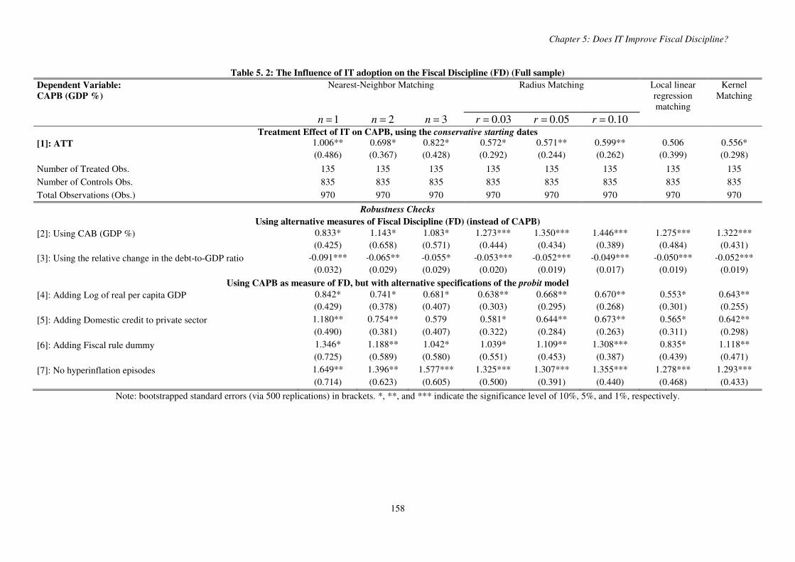
Chapter 5: Does IT Improve Fiscal Discipline?
158
Table 5. 2: The Influence of IT adoption on the Fiscal Discipline (FD) (Full sample)
Dependent Variable:
CAPB (GDP %)
Nearest-Neighbor Matching Radius Matching Local linear regression matching
Kernel Matching
1=n 2=n 3=n 03.0=r 05.0=r 10.0=r
Treatment Effect of IT on CAPB, using the conservative starting dates
[1]: ATT 1.006** 0.698* 0.822* 0.572* 0.571** 0.599** 0.506 0.556*
(0.486) (0.367) (0.428) (0.292) (0.244) (0.262) (0.399) (0.298)
Number of Treated Obs. 135 135 135 135 135 135 135 135
Number of Controls Obs. 835 835 835 835 835 835 835 835
Total Observations (Obs.) 970 970 970 970 970 970 970 970
Robustness Checks
Using alternative measures of Fiscal Discipline (FD) (instead of CAPB)
[2]: Using CAB (GDP %) 0.833* 1.143* 1.083* 1.273*** 1.350*** 1.446*** 1.275*** 1.322***
(0.425) (0.658) (0.571) (0.444) (0.434) (0.389) (0.484) (0.431)
[3]: Using the relative change in the debt-to-GDP ratio -0.091*** -0.065** -0.055* -0.053*** -0.052*** -0.049*** -0.050*** -0.052*** (0.032) (0.029) (0.029) (0.020) (0.019) (0.017) (0.019) (0.019)
Using CAPB as measure of FD, but with alternative specifications of the probit model
[4]: Adding Log of real per capita GDP 0.842* 0.741* 0.681* 0.638** 0.668** 0.670** 0.553* 0.643**
(0.429) (0.378) (0.407) (0.303) (0.295) (0.268) (0.301) (0.255)
[5]: Adding Domestic credit to private sector 1.180** 0.754** 0.579 0.581* 0.644** 0.673** 0.565* 0.642**
(0.490) (0.381) (0.407) (0.322) (0.284) (0.263) (0.311) (0.298)
[6]: Adding Fiscal rule dummy 1.346* 1.188** 1.042* 1.039* 1.109** 1.308*** 0.835* 1.118**
(0.725) (0.589) (0.580) (0.551) (0.453) (0.387) (0.439) (0.471)
[7]: No hyperinflation episodes 1.649** 1.396** 1.577*** 1.325*** 1.307*** 1.355*** 1.278*** 1.293***
(0.714) (0.623) (0.605) (0.500) (0.391) (0.440) (0.468) (0.433)
Note: bootstrapped standard errors (via 500 replications) in brackets. *, **, and *** indicate the significance level of 10%, 5%, and 1%, respectively.

Chapter 5: Does IT Improve Fiscal Discipline?
159
We investigate in the following the pertinence of our results, by accounting for eventual
differences in the group of developed, compared to the group of developing countries.
5.4.3. The effect of IT on FD: developed versus developing countries
We first analyze the effect of IT adoption on FD in the group of developed countries, which
consists of 22 countries, namely 8 ITers and 14 non-ITers. The results of the probit equations
used to compute propensity scores, presented in Appendix 5.B, are close to those performed
on the full sample (see Table 5.1 above), in terms of sign and significance of the estimated
coefficients. In particular, we find again that FD seems not to have exerted a significant effect
on the probability of adopting IT. These results remain robust when using different measures
for FD, when accounting for additional determinants of IT adoption, or when excluding
hyperinflation episodes (see regressions [1]-[7] in Appendix 5.B). Based on these propensity
scores, Table 5.3 illustrates the ATT of IT adoption on FD.
Compared to our findings for the full sample, results on line [1] of Table 5.3 below show that
the ATT of IT on FD is not statistically significant (although still with the positive sign) for
the group of developed countries. Using different measures of FD (see lines [2] and [3]),
adding additional variables (see lines [4] to [6]), or excluding hyperinflation episodes (see line
[7]) does not dramatically affects our findings.124 Consequently, although we detect some
signs of a FD improvement in developed countries following IT adoption, this effect is not
statistically significant. One possible explanation for the lack of a robust effect of IT on FD is
that, at the time the IT regime was adopted, developed countries presented already strong
fiscal institutions and a fiscal stance that was judged as sustainable by financial markets.
Since the fiscal stance prior to IT adoption was strong enough to support the good functioning
of, and the commitment to the IT framework, the pressure for performing important FD
reforms following the IT adoption is weak in these countries.
124 Except for some specifications (see line [5] in Table 5.3 and Appendix 5.C based on default starting dates).

Chapter 5: Does IT Improve Fiscal Discipline?
160
Table 5. 3: The Influence of IT on the Fiscal Discipline (FD) (Developed countries subsample)
Dependent Variable:
CAPB (GDP %)
Nearest-Neighbor Matching Radius Matching Local linear regression matching
Kernel Matching
1=n 2=n 3=n 03.0=r 05.0=r 10.0=r
Treatment Effect of IT on CAPB, using the conservative starting dates
[1]: ATT 0.868 1.490 1.278 0.788 1.293 0.992 1.129 1.308
(1.125) (0.988) (0.954) (0.938) (0.928) (0.789) (0.926) (1.024)
Number of Treated Obs. 80 80 80 78 78 78 80 80
Number of Controls Obs. 269 269 269 269 269 269 269 269
Total Observations (Obs.) 349 349 349 347 347 347 349 349
Robustness Checks
Using alternative measures of Fiscal Discipline (FD) (instead of CAPB)
[2]: Using CAB (GDP %) 0.887 0.497 0.294 0.486 0.704 0.586 0.512 0.699
(0.923) (0.874) (0.904) (0.672) (0.694) (0.571) (0.684) (0.588)
[3]: Using the relative change in the debt-to-GDP ratio -0.021 -0.012 -0.004 -0.014 -0.007 -0.014 -0.014 -0.009 (0.030) (0.027) (0.030) (0.023) (0.020) (0.016) (0.017) (0.019)
Using CAPB as dependent variable, but with alternative specifications of the probit model
[4]: Adding Log of real per capita GDP 0.374 0.132 0.0855 0.456 0.275 0.321 0.676 0.421
(1.129) (1.068) (0.944) (0.759) (0.854) (0.791) (0.997) (0.826)
[5]: Adding Domestic credit to private sector 1.786 1.735 1.823* 1.567* 1.569* 1.452* 1.350 1.614*
(1.263) (1.081) (1.018) (0.914) (0.932) (0.794) (0.926) (0.973)
[6]: Adding Fiscal rule dummy -0.994 -1.299 -0.844 -0.691 -1.392 -0.912 -1.132 -1.365
(1.215) (1.203) (1.249) (0.939) (1.110) (0.984) (1.092) (0.987)
[7]: No hyperinflation episodes 0.868 1.490 1.278 0.788 1.293 0.992 1.129 1.308
(0.855) (0.914) (1.073) (0.864) (0.906) (0.690) (0.805) (0.830)
Note: bootstrapped standard errors (via 500 replications) in brackets. *, **, and *** indicate the significance level of 10%, 5%, and 1%, respectively.

Chapter 5: Does IT Improve Fiscal Discipline?
161
Let now focus on the effect of IT on FD for the group of developing countries, which covers
62 countries, namely 18 ITers and 44 non-ITers. The analysis of probit regressions [1] in
Appendix 5.D reveals that, contrary to results for developed countries, the estimated
coefficient for the CAPB is positive and significant. The same holds when we consider
additional variables, when we abstract from hyperinflation episodes (see columns [4]-[7]), or
when we use the CAB as alternative measure of past fiscal performance (Column [2]).125
Consequently, we reveal that even though developing ITers adopted IT without having met
the fiscal prerequisites (see Amato & Gerlach, 2002; or Batini & Laxton, 2007), they had
better fiscal stances compared to developing countries non-ITers prior to IT adoption.
Based on these propensity scores, we display on line [1] of Table 5.4, the ATT of IT on the
FD (measured by the CAPB), which we find to be significantly positive in 7 out of the 8
considered cases. In addition, subsequent results reported on lines [2]-[3] confirm that our
findings are robust to alternative measures of FD. According to our estimations, the adoption
of full-fledged IT regimes increased the CAPB by a value ranging between 1.85 (for 3=n )
and 3.43 (for 1=n ) percentage points, the CAB by 1.30 (for local linear regression matching)
and up to 2.83 (for 1=n ) percentage points, and decreased the change in the public debt-to-
GDP ratio by a range between 16.0 (for local linear regression matching) and 24.3 (for 3=n )
percentage points.126
Moreover, we question the robustness of the significance and the size of these favorable
effects by presenting in the lower part of Table 5.4 matching results based on alternative
specifications for the computation of propensity scores. Irrespective of the additional
variables we consider, the ATT of IT on FD is positive and significant in at least 7 out of the 8
cases displayed on each of lines [4]-[6], a result which still holds when excluding
hyperinflation episodes on line [7]. In addition, the size of the positive effect on the CAPB is
comparable to its size in the benchmark case depicted on line [1], namely between 1.34
( 03.0=r on line [6]) and 3.40 (for 1=n on line [5]) percentage points. Finally, Appendix 5.E
illustrates that the favorable effect of IT on FD is qualitatively unchanged when accounting
for default, instead of conservative IT starting dates. 125 The change in the debt-to-GDP ratio is not found to significantly influence the IT adoption probability (see column [3], Appendix 5.D), while it turned to be significant when using the default starting dates (see column [3], Appendix 5.E.1); however, in both cases, IT adoption is found to have decreased the change in the debt-to-GDP ratio in ITers compared to non-ITers with comparable characteristics. 126 The sign of the ATT of IT on different measures of FD is still the same if we consider soft IT regimes based on default starting dates (see Appendix 5.E).

Chapter 5: Does IT Improve Fiscal Discipline?
162
Table 5. 4: The Influence of IT on the Fiscal Discipline (FD) (Developing countries subsample)
Dependent Variable:
CAPB (GDP %)
Nearest-Neighbor Matching Radius Matching Local linear regression matching
Kernel Matching
1=n 2=n 3=n 03.0=r 05.0=r 10.0=r
Treatment Effect of IT on CAPB, using the conservative starting dates
[1]: ATT 3.426** 1.747 1.853* 2.064** 2.068** 2.353** 3.279** 2.378** (1.590) (1.243) (1.119) (0.870) (1.042) (1.131) (1.343) (1.036) Number of Treated Obs. 55 55 55 41 45 51 55 48
Number of Controls Obs. 566 566 566 566 566 566 566 566
Total Observations (Obs.) 621 621 621 607 611 617 621 614
Robustness Checks
Using alternative measures of Fiscal Discipline (FD) (instead of CAPB)
[2]: Using CAB (GDP %) 2.831* 1.851 2.118** 1.313* 1.414* 1.243 1.299* 1.596* (1.446) (1.551) (1.080) (0.669) (0.721) (1.053) (0.773) (0.906) [3]: Using the relative change in the debt-to-GDP ratio -0.169* -0.203* -0.243** -0.180** -0.180** -0.181** -0.160** -0.181**
(0.100) (0.112) (0.107) (0.0874) (0.0888) (0.0727) (0.0809) (0.0921) Using CAPB as dependent variable, but with alternative specifications of the probit model
[4]: Adding Log of real per capita GDP 3.010** 2.560** 2.354** 2.048** 1.871* 1.932** 3.203** 2.042** (1.186) (1.243) (1.093) (0.932) (1.011) (0.873) (1.301) (1.019) [5]: Adding Domestic credit to private sector 3.403** 2.396** 2.155** 1.313 1.923* 2.390** 3.381** 2.188** (1.580) (1.166) (1.020) (0.908) (0.989) (1.027) (1.395) (0.973) [6]: Adding Fiscal rule dummy 1.823 2.616** 1.973** 1.340* 1.435* 1.497** 1.955* 1.406* (1.330) (1.210) (1.005) (0.705) (0.755) (0.764) (1.164) (0.851) [7]: No hyperinflation episodes 3.318** 1.755 1.835* 2.060** 2.075** 2.348** 3.326** 2.393** (1.686) (1.411) (1.028) (0.868) (1.043) (1.144) (1.358) (1.111)
Note: bootstrapped standard errors (via 500 replications) in brackets. *, **, and *** indicate the significance level of 10%, 5%, and 1%, respectively.

Chapter 5: Does IT Improve Fiscal Discipline?
163
The fact that IT adoption has a significant effect on FD only in developing countries is
undoubtedly related to the fact that these countries have specific structural characteristics,
which distinguish them from developed countries. In particular, developing countries present
weak institutions, and seigniorage revenues still represent a substantial share of government
revenue, making central banks less independent and less credible compared to central banks
in developed countries (see Masson et al., 1997; Calvo & Mishkin, 2003; or Jonas & Mishkin,
2004). In addition, many developing countries adopted IT despite displaying, at the time of IT
adoption, fiscal stances that were judged as doubtful in terms of sustainability, or simply poor
fiscal stance (compared to developed countries), as emphasized by Amato & Gerlach (2002)
or Batini & Laxton (2007). Consequently, a radical improvement in the FD is necessary
following the IT adoption, in order to send strong signals regarding the commitment of
authorities in meeting the target established by the IT monetary regime, and from a larger
standpoint, the commitment to preserve the IT viability.
5.5. Conclusion
The present chapter adds to the literature on the macroeconomic consequences of IT by
studying, for the first time to the best of our knowledge, the link between IT and fiscal
discipline (FD). Indeed, although the role of FD as a precondition for IT adoption was
previously analyzed, little is said about the way IT adoption could influence the FD. Using a
sample and an econometric method that allow comparability with previous studies focusing
on the IT performances, we develop the existing literature in several directions. First, based
on matching techniques applied on a sample of both developing and developed countries, we
show that IT adoption significantly improved FD in ITers compared to non-ITers with close
observable characteristics. Our result is extremely vigorous, in both sign and magnitude,
when performing different robustness tests, including alternative measures of FD, alternative
specifications for the computation of propensity scores, the use of conservative or default
starting dates for IT adoption, or a wide variety of matching methods. Consequently, we
extend the literature focusing on FD as a precondition for IT adoption, by showing that IT
adoption exerted a favorable effect on FD. Second, to deal with the possible heterogeneity in
our full sample, we investigate the role of IT adoption on FD by considering alternatively
developed and developing countries. Contrary to developed countries, where IT adoption does
not seem to have significantly improved FD (the effect we display presents the right sign but

Chapter 5: Does IT Improve Fiscal Discipline?
164
with little statistical significance), our results illustrate that developing countries having
adopted IT experienced a significant improvement in their fiscal stance. A possible
explanation of our findings builds on the idea that, contrary to developed countries,
developing countries were forced to improve their FD following IT adoption, in order to send
clear signals about their commitment to preserve the IT viability (i.e. the fear of missing the
inflation target urged their government to improve fiscal policy), given that at the time of the
adoption these developing countries presented unsustainable and/or poor fiscal stance (see,
e.g., Amato & Gerlach, 2002; or Batini & Laxton, 2007), and/or less independent and less
credible central banks compared to developed countries (see, e.g., Calvo & Mishkin, 2003; or
Jonas & Mishkin, 2004).
Finally, we provide an evaluation of the contribution of IT adoption to the improvement in
FD. According to our analysis, IT adoption alone led to a statistically significant gap between
ITers and non-ITers regarding all considered measures of FD, a gap which we estimate at as
high as +1.6 percentage points for the CAPB (+1.5 for the CAB and -9.1 percentage points for
the change in the debt-to-GDP ratio) if we consider the full sample, and +3.4 percentage
points for the CAPB (+2.8 for the CAB and -24.3 percentage points for the change in the
debt-to-GDP ratio) for the group of developing countries.
Our findings are particularly appealing as they may contribute to the discussion regarding the
performances of IT regimes, all the more that an impressive number of countries (more than
35, according to Batini et al., 2006, p.8), are currently exploring the possibility of
implementing IT frameworks. Indeed, in addition to previous studies having explored only the
role of FD as a prerequisite for a credible adoption of IT, our results suggest that the adoption
of an IT monetary regime enhances FD. Particularly for developing countries, IT appears as a
tool to “tie your own hands”, and could allow them to create a sound and stable
macroeconomic environment, which is, all the more in the current context of globalizing
financial markets, a key prerequisite for strong and sustained economic growth.
This finding that IT, a MP framework (as opposed to a fiscal policy framework) affects fiscal
authorities’ behaviors, then constitutes a fertile ground for assuming that MP and fiscal policy
frameworks should not be considered separately when it comes to assessing their
macroeconomic consequences. Their potential interactions need to be taken into account, an
issue that we address in the next chapter of the thesis.

Chapter 5: Does IT Improve Fiscal Discipline?
165
Appendices
Appendix 5.1: The list of the ITers, together with their starting dates
Countries Soft IT:
Default starting dates
Full-Fledged IT:
Conservative starting dates
Australia# March 1993 September 1994 Brazil* June 1999 June 1999
Canada# February 1991 January 1992 Chile* January 1991 August 1999
Colombia* September 1999 October 1999 Czech Republic* January 1998 January 1998
Finland# February 1993 January 1994 Hungary* June 2001 August 2001 Iceland# March 2001 March 2001 Israel* January 1992 June 1997
Mexico* January 1999 January 2001 New Zealand# March 1990 March 1990
Norway# March 2001 March 2001 Peru* January 2002 January 2002
Philippines* January 2002 January 2002 Poland* September 1998 September 1998
South Africa* February 2000 February 2000 South Korea* April 1998 April 1998
Spain# January 1995 January 1995 United Kingdom# October 1992 October 1992
Sweden# January 1993 January 1995 Switzerland# January 2000 January 2000
Thailand* May 2000 May 2000 New ITers (still treated as non-ITers in our study)
Indonesia* July 2005 July 2005 Romania* August 2005 August 2005
Slovak Republic* January 2005 January 2005 Guatemala* January 2005 January 2005
Turkey* January 2006 January 2006 Serbia* September 2006 September 2006 Ghana* January 2007 January 2007
Source: Rose (2007) and Roger (2009). Due to lack of data on fiscal discipline, Romania and Serbia do not appear in our sample. *: Developing Countries; #: Developed Countries.
Appendix 5.2: Control group (* Developing Countries; # Developed Countries)
Albania* Croatia* Ghana* Malta* Sri Lanka* Algeria* Cyprus* Greece# Malaysia* Swaziland*
Argentina* Germany# Guatemala* Mauritius* Trinidad and Tobago* Austria# Denmark# Ireland# Morocco* Tunisia*
Azerbaijan* Dominican Republic* Iran* Panama* Turkey* Belgium# Ecuador* Italy# Paraguay* Ukraine* Bulgaria* Egypt* Indonesia* Portugal# Uruguay* Bahrain* Estonia* Jamaica* Russian Federation* United States#
Bahamas* Finland# Jordan* El Salvador* Venezuela* Belarus* Fiji* Japan# Singapore*
Botswana* France# Kazakhstan* Slovak Republic* Cape Verde* Gabon* Latvia* Slovenia* Costa Rica* Georgia* Lithuania* Spain#

Chapter 5: Does IT Improve Fiscal Discipline?
166
Appendix 5.3: Sources and definitions of data
Public Debt (% of GDP) Gross General government debt, in percentage of GDP Ali Abbas et al. (2010) Change in the public debt-to-GDP
ratio Difference between current Debt/GDP and lagged
Debt/GDP, divided by lagged Debt/GDP. Authors’ calculations
CAPB Cyclically-Adjusted Primary fiscal Balance, as GDP
percentage. Authors’ calculations (see
Appendix 5.5), based on general government fiscal balances data
from WEO (2010) CAB
Cyclically-Adjusted fiscal Balance, as GDP percentage.
Full-Fledged or Formal IT (conservative starting dates)
Soft or Informal IT (default starting dates)
Binary variable taking the value 1 if in a given year a country operates formally under IT, zero otherwise.
When we use the conservative starting dates of IT, we refer to full-fledged IT.
Binary variable taking the value 1 if in a given year a country operates informally under IT, zero otherwise. When we use the default starting dates of IT, we refer
to soft IT.
Rose (2007) and Roger (2009)
Real per capita GDP growth rate
Real per capita GDP
Annual growth rate of real per capita output
GDP per capita at constant prices. Proxy for country’s level of economic development.
Penn World Table (PWT.6.3)
Trade openness Sum of imports and exports divided by GDP Inflation rate Annual growth rate of average CPI World Economic Outlook (2010)
Fiscal rule dummy
Binary variable taking the value 1 if a country placed, at the national level, a numerical limit on fiscal
aggregates (fiscal balance, expenditure, revenue or debt)
Fiscal Rules Database of the IMF’s Fiscal Affairs Department,
Fiscal Policy and Surveillance Division (2009)
Domestic credit to the private sector
Credit offered by domestic banks to private sector. Proxy for financial development or credit constraints
World Development Indicators (WDI, 2010)
Governors’ Turnover rate Central Banks Governors Turnover rates. Reverse
proxy of central bank independence. Ghosh et al. (2003)
Fixed Exchange rate Dummy variable taking the value 1 if a country is classified as having a de facto fixed exchange rate
regime (hard or soft peg). Reinhart & Rogoff (2004)
Appendix 5.4: Descriptive statistics
Variable Obs. Mean Std. Dev. Min. Max.
Full-Fledged IT 1978 0.111 0.314 0.000 1.000
Soft IT 1978 0.121 0.327 0.000 1.000
Inflation rate 1838 41.444 287.306 -11.374 7481.691
CAPB 1512 0.045 3.098 -14.006 21.569
CAB 1587 -0.055 3.546 -24.575 22.274
Debt (% of GDP) 1745 53.905 31.464 3.241 289.554
Change in the debt-to-GDP ratio 1633 0.002 0.205 -0.546 3.331
Fixed Exchange rate dummy 1816 0.572 0.495 0.000 1.000
Trade Openness 1871 80.638 50.651 10.094 456.562
Governor’s Turnover Rates 1478 0.245 0.236 0.000 1.200 Real per capita GDP growth rate 1857 2.549 4.735 -26.117 34.175
Log of real per capita GDP 1871 9.275 0.751 7.035 10.787
Fiscal rules Dummy variable 1978 0.257 0.437 0 1 Domestic credit to the private sector 1740 1797.849 15823.220 -72.994 194889.500

Chapter 5: Does IT Improve Fiscal Discipline?
167
Appendix 5.5: Computation of the Cyclically-Adjusted Primary fiscal Balance (CAPB)
For each country i of our sample, the CAPB is computed as the estimated residuals ( iε̂ ) of
the following country-specific equation (with t the time period)
iWOGPBPB it
it
it
it
it ∀++++= − ,1 εδγβα , (5.A1)
where PB denotes the primary fiscal balance127 in % of GDP, OG the output gap and W a
vector of control variables. As control variables, we include inflation and a time trend. For
each country, we compute the output gap as ( ) yyyOG tt /−= , where ty stands for the
logarithm of real per capita GDP in the year t , and y for the Hodrick-Prescott (HP) filtered
trend of ty . When applying the HP filter, despite a certain consensus for the use of a
smoothing parameter of 1600=λ for quarterly data (see the seminal paper of Hodrick &
Prescott, 1997, for a discussion), the related literature emphasized different values for λ for
annual data. According to Ravn & Uhlig (2002), if we consider that quarterly data are of
frequency 1, then annual data are of frequency 1/4, and the smoothing parameter for annual
data can be computed as ( ) 1600*4/1 n=λ , with n an integer. In our computations we follow
Ravn & Uhlig (2002), who recommend the value 4=n , leading to a smoothing parameter of
25.6=λ for annual data (results for 100=λ , corresponding to 2=n , as suggested by
Backus & Kehoe, 1992, do not lead to any qualitative change in our results and are available
upon request). The coefficient γ measures the cyclical response of fiscal policy to business
cycle fluctuations, and the error term tε measures the unsystematic component of fiscal
policy. The predicted value of this latter captures the part of the primary fiscal balance
unexplained by economic conditions, and is our main measure of fiscal discipline (CAPB).
Finally, to correct for a potential endogeneity of output gap in equation (5.A1), we use the
two stages least squares method (2SLS) estimator, in which we instrumented OG with its
lagged value and the growth rate of the terms of trade.
127 The same applies for the Cyclically-Adjusted fiscal Balance (CAB), in which case we consider the overall fiscal balance instead of the primary fiscal balance.

Chapter 5: Does IT Improve Fiscal Discipline?
168
Appendix 5.A: Full Sample, based on Default starting dates
Table 5.A.1: Probit estimates of the Propensity Scores (Full Sample)
Dependent variable: Inflation Targeting (Default Starting Dates)
[1] [2] [3] [4] [5] [6] [7]a
Inflation (lagged one year) -0.079*** -0.078*** -0.073*** -0.073*** -0.078*** -0.065*** -0.078*** (0.010) (0.009) (0.009) (0.012) (0.010) (0.010) (0.010) Governors’ turnover rate -0.600* -0.584* -0.710** -0.579* -0.612* -0.589* -0.590* (0.336) (0.329) (0.310) (0.340) (0.329) (0.346) (0.337) Debt/GDP (lagged one year) -0.006*** -0.007*** -0.005*** -0.006*** -0.005** -0.007*** -0.006*** (0.002) (0.002) (0.002) (0.002) (0.002) (0.002) (0.002) Real per capita GDP growth rate 0.027* 0.027* 0.014 0.027* 0.023 0.026* 0.026* (0.015) (0.015) (0.014) (0.015) (0.015) (0.015) (0.015) Fixed Exchange rate dummy -1.507*** -1.535*** -1.448*** -1.486*** -1.461*** -1.470*** -1.507*** (0.124) (0.123) (0.117) (0.125) (0.128) (0.124) (0.124) Trade Openness -0.006*** -0.006*** -0.004*** -0.006*** -0.006*** -0.004*** -0.006*** (0.001) (0.001) (0.001) (0.001) (0.001) (0.001) (0.001) CAPB (lagged one year) 0.012 0.012 0.016 -0.001 0.012 (0.020) (0.020) (0.019) (0.020) (0.020) CAB (lagged one year 0.015 (0.019) Debt Change (lagged one year) -0.369 (0.329) Log of real per capita GDP 0.085 (0.099) Domestic credit to private sector -2.01e-06 (2.22e-06) Fiscal rule dummy 0.456*** (0.140) Constant 1.055*** 1.106*** 0.848*** 0.188 1.037*** 0.757*** 1.049*** (0.181) (0.177) (0.162) (1.037) (0.183) (0.190) (0.181) Number of observations 982 1030 1140 982 923 982 914 Pseudo R2 0.333 0.343 0.313 0.334 0.331 0.345 0.314
a Excluding hyperinflation episodes. Robust standard errors in brackets. *, **, and *** indicate the significance level of 10%, 5%, and 1%. CAPB and CAB refer to the Cyclically-Adjusted Primary, and respectively overall, fiscal Balance, both as GDP percentage.

Chapter 5: Does IT Improve Fiscal Discipline?
169
Table 5.A.2: The Influence of IT adoption on the Fiscal Discipline (FD) (Full sample)
Dependent Variable :
CAPB (GDP %)
Nearest-Neighbor Matching Radius Matching Local linear regression matching
Kernel Matching
1=n 2=n 3=n 03.0=r 05.0=r 10.0=r
Treatment Effect of IT on CAPB, using the default starting dates
[1]: ATT 0.913* 0.450 0.339 0.605** 0.609** 0.553** 0.505* 0.605**
(0.519) (0.424) (0.421) (0.280) (0.306) (0.270) (0.258) (0.292)
Number of Treated Obs. 142 142 142 142 142 142 142 142
Number of Controls Obs. 820 820 820 820 820 820 820 820 Total Observations (Obs.) 962 962 962 962 962 962 962 962
Robustness Checks
Using alternative measures of fiscal discipline (instead of CAPB) as measure of Fiscal Discipline (FD)
[2]: Using CAB (GDP %) 1.108 1.659*** 1.573** 1.182*** 1.141*** 1.231*** 1.003** 1.120***
(0.850) (0.608) (0.738) (0.453) (0.402) (0.358) (0.433) (0.414) [3]: Using the relative Change in the Debt-to GDP ratio -0.040 -0.043* -0.055* -0.058*** -0.058*** -0.059*** -0.056*** -0.058***
(0.038) (0.022) (0.030) (0.020) (0.016) (0.017) (0.017) (0.017)
Using CAPB as dependent variable, but with alternative specifications of the probit model
[4]: Adding Log of real per capita GDP 0.949* 0.672* 0.762* 0.475* 0.499* 0.533* 0.434* 0.473*
(0.549) (0.354) (0.451) (0.250) (0.262) (0.281) (0.221) (0.241)
[5]: Adding Domestic credit to private sector 0.952 1.265** 1.147* 1.286*** 1.445*** 1.475*** 1.294*** 1.400***
(0.749) (0.598) (0.601) (0.488) (0.428) (0.373) (0.423) (0.418)
[6]: Adding Fiscal rule dummy 1.517** 0.690 0.704* 0.798** 0.827** 0.877*** 0.616** 0.839***
(0.593) (0.529) (0.359) (0.350) (0.323) (0.269) (0.310) (0.324)
[7]: No hyperinflation episodes 1.926*** 1.621*** 1.479** 1.512*** 1.507*** 1.462*** 1.433*** 1.514***
(0.669) (0.612) (0.579) (0.423) (0.445) (0.407) (0.394) (0.396)
Note: bootstrapped standard errors (via 500 replications) in brackets. *, **, and *** indicate the significance level of 10%, 5%, and 1%, respectively.

Chapter 5: Does IT Improve Fiscal Discipline?
170
Appendix 5.B: Probit estimates of the Propensity Scores (Developed Countries)
Dependent variable : Inflation Targeting (Conservative Starting Dates)
[1] [2] [3] [4] [5] [6] [7]a
Inflation (lagged one year) -0.189*** -0.203*** -0.155*** -0.253*** -0.213*** -0.158*** -0.189*** (0.057) (0.055) (0.052) (0.062) (0.061) (0.061) (0.057) Governors’ turnover rate -1.612** -1.688*** -1.471** -1.536** -1.574** -1.771*** -1.612** (0.636) (0.642) (0.586) (0.646) (0.613) (0.666) (0.636) Debt/GDP (lagged one year) -0.012*** -0.013*** -0.010*** -0.013*** -0.013*** -0.014*** -0.012*** (0.003) (0.003) (0.003) (0.003) (0.003) (0.003) (0.003) Real per capita GDP growth rate 0.055 0.057 0.034 0.042 0.034 0.048 0.055 (0.036) (0.037) (0.035) (0.035) (0.037) (0.038) (0.036) Fixed Exchange rate dummy -1.078*** -1.082*** -0.970*** -1.340*** -0.949*** -1.053*** -1.078*** (0.193) (0.194) (0.189) (0.212) (0.214) (0.194) (0.193) Trade Openness 0.006** 0.006** 0.006** 0.007** 0.009** 0.007** 0.006** (0.003) (0.003) (0.003) (0.003) (0.003) (0.003) (0.003) CAPB (lagged one year) -0.031 -0.032 -0.024 -0.066 -0.031 (0.038) (0.036) (0.037) (0.041) (0.038) CAB (lagged one year) -0.064 (0.041) Debt Change (lagged one year) -0.786 (1.017) Log of real per capita GDP -1.588*** (0.447) Domestic credit to private sector 1.63e-06 (2.75e-06) Fiscal rule dummy 0.650*** (0.212) Constant 0.883*** 0.930*** 0.580** 17.37*** 0.892*** 0.472 0.883*** (0.302) (0.297) (0.285) (4.713) (0.332) (0.346) (0.302) Number of observations 354 358 365 354 296 354 354 Pseudo R2 0.260 0.270 0.223 0.291 0.250 0.288 0.260
a Excluding hyperinflation episodes. Robust standard errors in brackets. *, **, and *** indicate the significance level of 10%, 5%, and 1%. CAPB and CAB refer to the Cyclically-Adjusted Primary, and respectively overall, fiscal Balance, both as GDP percentage.

Chapter 5: Does IT Improve Fiscal Discipline?
171
Appendix 5.C: Developed Countries, based on Default starting dates
Table 5.C.1: Probit estimates of the Propensity Scores (Developed Countries)
Dependent variable: Inflation Targeting (Default Starting Dates)
[1] [2] [3] [4] [5] [6] [7]a
Inflation (lagged one year) -0.194*** -0.214*** -0.145*** -0.270*** -0.218*** -0.170*** -0.194*** (0.054) (0.052) (0.048) (0.059) (0.058) (0.058) (0.054) Governors’ turnover rate -1.692*** -1.723*** -1.394** -1.636** -1.656*** -1.844*** -1.692*** (0.636) (0.629) (0.564) (0.647) (0.614) (0.665) (0.636) Debt/GDP (lagged one year) -0.013*** -0.013*** -0.011*** -0.014*** -0.014*** -0.014*** -0.013*** (0.003) (0.003) (0.003) (0.003) (0.003) (0.003) (0.003) Real per capita GDP growth rate 0.020 0.017 0.010 0.007 0.001 0.011 0.020 (0.037) (0.038) (0.036) (0.036) (0.038) (0.039) (0.037) Fixed Exchange rate dummy -1.071*** -1.081*** -1.012*** -1.402*** -0.946*** -1.046*** -1.071*** (0.192) (0.194) (0.190) (0.211) (0.213) (0.193) (0.192) Trade Openness 0.006** 0.007** 0.007*** 0.007*** 0.009*** 0.007** 0.006** (0.003) (0.003) (0.003) (0.003) (0.003) (0.003) (0.003) CAPB (lagged one year) -0.074* -0.075* -0.065* -0.108** -0.074* (0.040) (0.038) (0.039) (0.042) (0.040) CAB (lagged one year) -0.094** (0.041) Debt Change (lagged one year) 0.848 (0.879) Log of real per capita GDP -1.924*** (0.455) Domestic credit to private sector 1.22e-06 (2.70e-06) Fiscal rule dummy 0.548*** (0.200) Constant 1.031*** 1.123*** 0.621** 21.01*** 1.023*** 0.702** 1.031*** (0.293) (0.289) (0.274) (4.785) (0.320) (0.336) (0.293) Number of observations 354 358 365 354 296 354 354 Pseudo R2 0.260 0.270 0.215 0.304 0.250 0.280 0.260
a Excluding hyperinflation episodes. Robust standard errors in brackets. *, **, and *** indicate the significance level of 10%, 5%, and 1%. CAPB and CAB refer to the Cyclically-Adjusted Primary, and respectively overall, fiscal Balance, both as GDP percentage.

Chapter 5: Does IT Improve Fiscal Discipline?
172
Table 5.C.2: The Influence of IT adoption on the Fiscal Discipline (FD) (Developed Countries)
Dependent Variable :
CAPB (GDP %)
Nearest-Neighbor Matching Radius Matching Local linear regression matching
Kernel Matching
1=n 2=n 3=n 03.0=r 05.0=r 10.0=r
Treatment Effect of IT on CAPB, using the default starting dates
[1]: ATT 1.086 1.310 1.401* 1.280* 1.330* 1.178* 1.274* 1.371*
(0.927) (1.030) (0.841) (0.754) (0.741) (0.682) (0.713) (0.778)
Number of Treated Obs. 85 85 85 77 77 77 85 77
Number of Controls Obs. 264 264 264 264 264 264 264 264 Total Observations (Obs.) 349 349 349 341 341 341 349 341
Robustness Checks
Using alternative measures of fiscal discipline (instead of CAPB) as measure of Fiscal Discipline (FD)
[2]: Using CAB (GDP %) 1.129 1.407* 1.614* 1.569* 1.622* 1.220 0.731 1.564**
(0.944) (0.840) (0.931) (0.807) (0.896) (0.792) (0.831) (0.798) [3]: Using the relative Change in the Debt-to GDP ratio -0.027 -0.033 -0.033 -0.031 -0.034 -0.025 -0.026 -0.033
(0.036) (0.026) (0.027) (0.023) (0.021) (0.018) (0.019) (0.022)
Using CAPB as dependent variable, but with alternative specifications of the probit model
[4]: Adding Log of real per capita GDP 0.410 -0.412 -0.340 0.420 0.0812 0.0775 -0.478 0.0466
(1.299) (1.219) (1.101) (0.729) (0.926) (0.893) (1.359) (0.995)
[5]: Adding Domestic credit to private sector 1.506 1.653* 1.980** 1.542** 1.519** 1.385** 1.336 1.529
(1.055) (0.999) (0.856) (0.728) (0.749) (0.687) (0.986) (1.017)
[6]: Adding Fiscal rule dummy 0.966 1.949 0.657 0.442 0.407 -0.180 0.295 0.363
(1.367) (1.189) (0.916) (0.819) (1.006) (1.001) (1.036) (0.951)
[7]: No hyperinflation episodes 1.086 1.310 1.401 1.280** 1.330* 1.178** 1.274 1.371**
(0.824) (0.964) (0.897) (0.624) (0.713) (0.567) (0.844) (0.671)
Note: bootstrapped standard errors (via 500 replications) in brackets. *, **, and *** indicate the significance level of 10%, 5%, and 1%, respectively.

Chapter 5: Does IT Improve Fiscal Discipline?
173
Appendix 5.D: Probit estimates of the Propensity Scores (Developing Countries)
Dependent variable: Inflation Targeting (Conservative Starting Dates)
[1] [2] [3] [4] [5] [6] [7]a
Inflation (lagged one year) -0.148*** -0.147*** -0.131*** -0.143*** -0.144*** -0.139*** -0.148*** (0.020) (0.020) (0.017) (0.019) (0.020) (0.020) (0.020) Governors’ turnover rate -1.548*** -1.576*** -1.251** -1.594*** -1.579*** -1.641*** -1.544*** (0.499) (0.496) (0.505) (0.484) (0.508) (0.525) (0.500) Debt/GDP (lagged one year) -0.008** -0.008** -0.007** -0.006* -0.009** -0.009** -0.008** (0.004) (0.003) (0.003) (0.003) (0.004) (0.004) (0.004) Real per capita GDP growth rate 0.008 0.009 -0.005 0.006 0.010 0.006 0.008 (0.023) (0.022) (0.019) (0.022) (0.023) (0.022) (0.023) Fixed Exchange rate dummy -2.551*** -2.500*** -2.192*** -2.484*** -2.497*** -2.519*** -2.550*** (0.335) (0.307) (0.257) (0.300) (0.329) (0.347) (0.335) Trade Openness -0.012*** -0.012*** -0.008*** -0.014*** -0.013*** -0.011*** -0.012*** (0.003) (0.002) (0.002) (0.003) (0.003) (0.002) (0.003) CAPB (lagged one year) 0.102*** 0.099*** 0.102*** 0.094*** 0.102*** (0.030) (0.030) (0.031) (0.031) (0.030) CAB (lagged one year) 0.095*** (0.030) Debt Change (lagged one year) -0.163 (0.287) Log of real per capita GDP 0.292 (0.242) Domestic credit to private sector 0.003 (0.002) Fiscal rule dummy 0.609*** (0.228) Constant 2.569*** 2.513*** 1.759*** -0.129 2.368*** 2.280*** 2.566*** (0.430) (0.400) (0.307) (2.113) (0.447) (0.421) (0.431) Number of observations 628 672 775 628 627 628 560 Pseudo R2 0.512 0.509 0.459 0.516 0.515 0.526 0.494
a Excluding hyperinflation episodes. Robust standard errors in brackets. *, **, and *** indicate the significance level of 10%, 5%, and 1%. CAPB and CAB refer to the Cyclically-Adjusted Primary, and respectively overall, fiscal Balance, both as GDP percentage.

Chapter 5: Does IT Improve Fiscal Discipline?
174
Appendix 5.E: Developing Countries, based on Default starting dates
Table 5.E.1: Probit estimates of the Propensity Scores (Developing Countries)
Dependent variable: Inflation Targeting (Default Starting Dates)
[1] [2] [3] [4] [5] [6] [7]a
Inflation (lagged one year) -0.119*** -0.119*** -0.096*** -0.112*** -0.112*** -0.112*** -0.119*** (0.019) (0.018) (0.014) (0.019) (0.019) (0.019) (0.019) Governors’ turnover rate -0.993** -1.032** -0.791* -1.163** -1.110** -1.032** -0.985** (0.486) (0.487) (0.439) (0.453) (0.487) (0.494) (0.489) Debt/GDP (lagged one year) -0.008** -0.009*** -0.006** -0.004 -0.010*** -0.008** -0.008** (0.003) (0.003) (0.003) (0.003) (0.003) (0.003) (0.003) Real per capita GDP growth rate 0.041* 0.045* 0.023 0.035 0.044* 0.040* 0.041* (0.024) (0.024) (0.020) (0.023) (0.024) (0.023) (0.024) Fixed Exchange rate dummy -2.654*** -2.678*** -2.282*** -2.546*** -2.592*** -2.613*** -2.652*** (0.358) (0.342) (0.244) (0.333) (0.356) (0.357) (0.358) Trade Openness -0.013*** -0.013*** -0.009*** -0.016*** -0.014*** -0.012*** -0.013*** (0.003) (0.002) (0.002) (0.003) (0.003) (0.002) (0.003) CAPB (lagged one year) 0.105*** 0.102*** 0.112*** 0.100*** 0.105*** (0.029) (0.029) (0.031) (0.029) (0.029) CAB (lagged one year) 0.106*** (0.030) Debt Change (lagged one year) -0.859** (0.402) Log of real per capita GDP 0.619** (0.270) Domestic credit to private sector 0.006*** (0.002) Fiscal rule dummy 0.374* (0.223) Constant 2.449*** 2.479*** 1.583*** -3.186 2.123*** 2.235*** 2.441*** (0.439) (0.416) (0.294) (2.326) (0.457) (0.432) (0.441) Number of observations 628 672 775 628 627 628 560 Pseudo R2 0.511 0.522 0.452 0.530 0.523 0.516 0.492
a Excluding hyperinflation episodes. Robust standard errors in brackets. *, **, and *** indicate the significance level of 10%, 5%, and 1%. CAPB and CAB refer to the Cyclically-Adjusted Primary, and respectively overall, fiscal Balance, both as GDP percentage.

Chapter 5: Does IT Improve Fiscal Discipline?
175
Table 5.E.2: The Influence of IT adoption on the Fiscal Discipline (FD) (Developing Countries)
Dependent Variable :
CAPB (GDP %)
Nearest-Neighbor Matching Radius Matching Local linear regression matching
Kernel Matching
1=n 2=n 3=n 03.0=r 05.0=r 10.0=r
Treatment Effect of IT on CAPB, using the default starting dates
[1]: ATT 3.738** 3.036** 1.975* 2.295** 2.287** 1.524* 3.227** 2.394**
(1.821) (1.479) (1.012) (0.903) (1.031) (0.781) (1.490) (1.144)
Number of Treated Obs. 55 55 55 50 51 55 55 52
Number of Controls Obs. 566 566 566 556 566 566 566 556
Total Observations (Obs.) 621 621 621 606 607 611 621 608
Robustness Checks
Using alternative measures of fiscal discipline (instead of CAPB) as measure of Fiscal Discipline (FD)
[2]: Using CAB (GDP %) 1.988 2.646* 2.642** 1.721** 1.685 1.124 1.641* 2.033**
(1.455) (1.516) (1.305) (0.843) (1.011) (0.892) (0.960) (0.966) [3]: Using the relative Change in the Debt-to GDP ratio -0.175** -0.174** -0.146** -0.178** -0.166*** -0.141*** -0.139** -0.162***
(0.0892) (0.0784) (0.0673) (0.0770) (0.0578) (0.0511) (0.0577) (0.0597) Using CAPB as dependent variable, but with alternative specifications of the probit model
[4]: Adding Log of real per capita GDP 1.810 0.927 2.592* 1.355* 1.215* 1.089* 1.514** 1.154*
(2.044) (1.703) (1.471) (0.702) (0.687) (0.555) (0.731) (0.588)
[5]: Adding Domestic credit to private sector 5.108*** 3.518** 2.771** 3.112*** 3.248*** 3.041** 4.459** 3.319***
(1.798) (1.647) (1.349) (1.041) (1.160) (1.235) (1.832) (1.170)
[6]: Adding Fiscal rule dummy 3.008*** 1.521* 1.439* 1.656* 1.644** 1.243 1.304** 1.441**
(0.823) (0.865) (0.784) (0.847) (0.768) (0.969) (0.631) (0.681)
[7]: No hyperinflation episodes 3.489** 3.082** 1.975* 2.188** 2.214** 1.456 3.356** 2.376**
(1.751) (1.548) (1.089) (0.942) (1.049) (1.078) (1.547) (1.064)
Note: bootstrapped standard errors (via 500 replications) in brackets. *, **, and *** indicate the significance level of 10%, 5%, and 1%, respectively.

Chapter 5: Does IT Improve Fiscal Discipline?
176
Appendix 5.F: The balancing properties of the matched data
Variables Sample Mean Standardized bias t-test
Treated Control % bias t p>t
Lagged inflation rate Unmatched 5,7282 77,205 -23 -1,2 0,23
Matched 6,5527 13,094 -2,1 -0,29 0,774
Governors’ turnover rate Unmatched 0,14136 0,22773 -44,9 -4,15 0
Matched 0,14726 0,14616 0,6 0,05 0,959
Lagged debt-to-GDP Unmatched 42,172 53,83 -45,5 -2,75 0,006
Matched 45,795 45,779 0,1 0 0,997
Real per capita GDP growth rate Unmatched 2,0912 2,4583 -8,7 -0,55 0,585
Matched 2,0701 2,1427 -1,7 -0,07 0,945
Fixed exchange rate Unmatched 0,10909 0,63748 -130 -7,98 0
Matched 0,15789 0,14534 3,1 0,15 0,881
Trade openness Unmatched 71,876 89,364 -35,8 -2,13 0,034
Matched 71,822 71,959 -0,3 -0,02 0,987
Lagged CAPB Unmatched 0,02893 -0,055 2,8 0,17 0,867
Matched 0,17149 0,08663 2,8 0,14 0,886
Log of real per capita GDP Unmatched 9,2185 8,9563 48,5 3,13 0,002
Matched 9,018 9,045 -5 -0,23 0,818
Domestic credit to the private sector Unmatched 75,104 51,591 55,2 4,09 0
Matched 61,518 61,018 1,2 0,07 0,944
Fiscal rule dummy Unmatched 0,59848 0,18438 93,5 10,87 0
Matched 0,57258 0,55682 3,6 0,25 0,803

177

178

179
Chapter 6
Inflation Targeting and Fiscal Rules:
Do Interactions and Sequence
of Adoption Matter?

Chapter 6. IT and FRs: Do Interactions and Sequence of Adoption Matter?
180
6.1. Introduction
This chapter is concerned with filling a gap in the existing literature on the effects of Inflation
Targeting (IT) and Fiscal Rules (FR), namely the failure of taking into account the influence
of likely interactions between IT and FR when it comes to assessing their respective
macroeconomic performances. Indeed, previous studies evaluated the respective effects of IT
and FR separately. On the fiscal side, a substantial strand of empirical literature emphasized
that FR are effective in delivering fiscal discipline (Alesina & Perotti, 1995; Alesina et al.,
1999; Debrun et al., 2007a; Hallerberg et al., 2009; Dabla-Norris et al., 2010; or Gollwitzer,
2011). On the monetary side, IT adoption was found successful in bringing down inflation
and its volatility, notably in developing countries (Batini & Laxton, 2007; Gonçalves &
Salles, 2008; Lin & Ye, 2009; or de Mendonça & de Guimarães e Souza, 2012).
However, a common drawback to both sets of studies is that papers having assessed the fiscal
impact of FR (the inflationary impacts of IT) did not take into account the potential effects of
IT on fiscal behaviors (of FR on inflation dynamics). On the one hand, the discipline-
enhancing effects on the conduct of fiscal policy attributed to FR may also stem partly from
IT adoption, as the latter may serve as a catalyst for the implantation of sound fiscal policies.
Indeed, Mishkin (2004), Roger (2009) or Freedman & Ötker-Robe (2010) defend the idea
that, to prevent the central bank from missing its inflation target due to pressure from the
government to monetize the public debt, IT adoption may be sufficiently binding for both the
central bank and the government to serve as a good device to ensure fiscal discipline. On the
other hand, fiscal discipline has been identified as a key prerequisite for the effectiveness of
IT in achieving price stability (Masson et al., 1997; Bernanke & Woodford, 2004; or Sims,
2004). Given that FR adoption is considered as a pivotal element in setting off fiscal
discipline, the favorable inflationary effects attributed to IT in the literature may also be partly
related to the presence of FR, rendering more credible the IT framework regarding the private
sector’s inflation expectations.
Consequently, there are good arguments for assuming that studying the effects of IT and FR
respectively on inflation and on fiscal balances without taking into account the influence of
interactions between them can lead to misleading conclusions. Such a reasoning is all the
more welcomed that IT (or FR) was sometimes adopted as part of broader reforms aiming at
strengthening macroeconomic stability; for instance, IT adoption sometimes went along with

Chapter 6. IT and FRs: Do Interactions and Sequence of Adoption Matter?
181
the introduction of bold fiscal reforms, including the establishment of FR, to support the IT
framework (for example in Brazil, Norway, New Zealand or Sweden). In some countries (for
instance in Brazil, Chile, Israel, Norway, Poland, Romania, or United Kingdom), legislation
measures prohibiting monetization of public debt, which are a form of FR, were adopted to
ensure the credibility of the commitment to the inflation target, while in other countries (such
as Australia, Canada, Czech Republic, Ghana, Indonesia, New Zealand, Philippines, South
Africa, or Turkey), the inflation target is jointly defined by the central bankers and the
government, to clearly signal to the financial markets that both fiscal and monetary authorities
are committed to hit the inflation target. Altogether, these arguments point out that the
effectiveness of IT and FR in affecting inflation and the fiscal stance may depend on whether
IT (FR) is implemented alone or jointly with the introduction of FR (IT). Put differently,
interactions between these rule-based policy frameworks seem to matter on their individual
inflationary and fiscal effects.
An additional motivation for our analysis stems from the fact that both IT and FR are rule-
based policy frameworks with the same ultimate goal, namely conferring credibility to
macroeconomic policies in general, as stressed out by Kopits (2001); as such, they may act
complementarily in achieving that common ultimate goal, all the more that both frameworks
experience concomitantly a growing popularity since the early nineties. Furthermore, both IT
and FR display many similarities in their nature, as they are defined in the form of numerical
targets on macroeconomic aggregates, namely on inflation for IT and on fiscal variables for
FR, with the goal of constraining the discretion of monetary and fiscal authorities,
respectively.128
Given this marked parallelism in the implementation of both frameworks, it is reasonable to
explore the likely role of their interactions when it comes to isolating their respective causal
effects on inflation dynamics and fiscal behaviors. From a broader viewpoint, the influence of
the interactions between IT and FR can be linked to the bourgeoning literature on the price
level determinacy, inspired by the seminal paper by Sargent & Wallace (1981), or the more
recent fiscal theory of the price level (Woodford, 1994). This literature (see, e.g., Aiyagari &
Gertler, 1985; Sims, 1988; Leeper, 1991; Benhabib et al., 2001; Uribe, 2006; or Sims, 2011)
128 In addition, IT and FR equally display similarities in their institutional parameters, as illustrated in the comparative description of their main features (see Appendix 6.1). Indeed, as pointed out by Kopits (2001), the new wave of FR, started in New Zealand in 1994, is backed up by institutional parameters which are also present in IT frameworks, such as transparency and accountability mechanisms.

Chapter 6. IT and FRs: Do Interactions and Sequence of Adoption Matter?
182
is interested in disentangling the relative importance of MP versus fiscal policy when it comes
to providing the nominal anchor to the economy. Accordingly, by pointing out that fiscal
(monetary) policy may alter the way monetary (fiscal) policy affects inflation dynamics, these
authors laid the foundations for taking into account the role of the interactions between
monetary and fiscal policies regarding their respective macroeconomic effects.129
In light of this literature, we question in this chapter, the interactions between IT and FR in
terms of their effects on inflation and fiscal balances, by focusing on two issues. First, we
explore if the joint effects of IT and FR on inflation and fiscal balances are larger compared to
their isolate effects. Second, we investigate the role of the sequence (or timing) of IT and FR
adoption, namely do interactions between IT and FR influence differently inflation and/or
fiscal balances depending on whether a country adopts IT before introducing FR, or
inversely?130 To this end, we perform System-GMM estimations, which properly address the
likely endogeneity in the adoption of both IT and FR and in their interactions and sequence of
adoption, and account for the inertia in the inflation dynamics and in the budget process, on a
panel of 152 developed and developing countries over the period 1990-2009. First, we find
that adopting both IT and FR improves fiscal balances and brings down average inflation
more than compared to the cases where only FR or only IT are adopted. Second, we highlight
the dominance of the sequence which consists of introducing first FR before adopting IT with
respect to the opposite sequence, regarding their fiscal and inflationary performances.
The rest of the chapter is organized as follows. Section 2 presents the dataset and displays
some stylized facts. Section 3 discusses the methodology and the estimation technique.
Section 4 illustrates the main results and their robustness, and section 5 concludes.
129 To characterize cases in which fiscal policy, rather than MP, may provide the nominal anchor to the economy, Sargent & Wallace (1981) distinguish two policy regimes, namely “monetary dominance” and “fiscal dominance” (these regimes are sometimes called “Ricardian” and “non-Ricardian” respectively, or “active” (passive) fiscal policy and “passive” (active) monetary policy respectively, see, Leeper, 1991, or Woodford, 1994). Under a fiscal dominance regime, the primary fiscal balance evolves independently of the public debt, causing the equilibrium level of price to raise in order to ensure government’s fiscal solvency; in this case, the nominal anchor is provided by fiscal policy, meaning that a restrictive MP may even result in higher inflation if the main source of government funding is seigniorage, and if the primary fiscal balance is not adjusted after seigniorage receipts collapse. On the contrary, under monetary dominance the primary fiscal balance evolves consistently with government’s fiscal solvency, so that the equilibrium price level is determined according to the traditional way, namely through the interaction between the supply and the demand for money. 130 A comparable strategy was adopted for exploring the complementarities and the optimal order of financial liberalization reforms (see, e.g., Dewatripont & Roland, 1995; or de Macedo & Martins, 2008) or political liberalization versus economic liberalization reforms (see Giavazzi & Tabellini, 2005).

Chapter 6. IT and FRs: Do Interactions and Sequence of Adoption Matter?
183
6.2. Data and Stylized Facts
We built upon a wide panel of 152 countries, covering both developed and developing
countries, over the period 1990-2009 (see Appendix 6.2 for the list of countries). The number
of countries in the sample is limited exclusively on the basis of data availability, especially
regarding outcome variables, namely fiscal balances (primary or overall) and the inflation
rate.131 Regarding the time coverage, the sample starts in 1990 because reliable fiscal data
exist only from 1990, all the more in developing countries, which are largely present in our
sample.
6.2.1. Variables of interest: Inflation Targeting and Fiscal Rules
IT is measured by a binary variable equaling one if at a given year a country uses IT as its
framework for the conduct of MP, and zero otherwise. Data on the starting dates of IT come
from Rose (2007), and were updated from Roger (2009) for recent experiences of IT
adoption, namely between 2005 and 2009. Rose (2007) distinguishes two kinds of dates,
namely default starting years and conservative starting years.132 For robustness issues, we
perform our analysis on both dates in the following sections. Among the 152 countries in the
sample, 29 experienced IT by the end of 2009 (see the first column of Appendix 6.3 for the list
of the 29 ITers along with their starting dates).133
We measure FR by a binary variable taking the value one if at a given year a country placed a
numerical constraint on fiscal aggregates (budget balance, spending, revenue or debt) at the
national level. Data on the starting dates of FR come from the new Fiscal Rules Database
(IMF’s Fiscal Affairs Department, Fiscal Policy and Surveillance Division, 2009), providing a
comprehensive overview on FR experiences around the world. Among the 152 countries in
the sample, 51 enacted Fiscal Rules (FRers) by the end of 2009 (see the second column of
Appendix 6.3 for the list of 51 FRers and their starting dates).134
131 Note that the panel is unbalanced because of missing observations. 132 The conservative starting dates refer to a form of IT termed “FFIT” while the default ones refer to “soft” IT. See Chapter 1, section 1.2.1 for further discussion on this issue. 133 Serbia adopted IT in 2006, but due to lack of data on fiscal balance, this country is dropped from the sample. Remark that three countries, namely Finland, Spain and Slovak Republic, adopted IT in 1993, 1995 and 2005 respectively, but the first two abandoned IT to join the Euro area in 1999, while the third did so in 2009. Consequently, we consider them as ITers only from their IT adoption date to their entrance date to the Euro area. 134 Armenia, Comoros, Hong Kong, Liberia, and Timor-Leste enacted FR in 2008, 2001, 1997, 2004 and 2005 respectively, but due to lack of data on fiscal balances and/or inflation they are dropped from our sample.

Chapter 6. IT and FRs: Do Interactions and Sequence of Adoption Matter?
184
6.2.2. The interaction between IT and FR and the sequence of adoption
To explore the potential impact of the interaction between IT and FR and of the timing
(sequence) of adoption of IT and FR, we build the five following dummy variables (see
columns three to seven of Appendix 6.3):
(i) A binary variable, called IT_only, equaling one after IT adoption in countries having
adopted only IT (these countries should have not adopted FR throughout the entire time
coverage of the sample, namely 1990-2009), and zero otherwise. For example, South
Africa adopted IT in 2000 and did not experience FR at all over 1990-2009; accordingly,
for South Africa, IT_only equals zero for 1990-1999, and one for 2000-2009;
(ii) A binary variable, called FR_only, equaling one after FR adoption in countries having
only enacted FR (these countries should have not adopted IT throughout the entire time
period of the sample, namely 1990-2009), and zero otherwise. For example, India
adopted FR in 2004 and did not experience IT at all over 1990-2009; accordingly, for
India, FR_only equals zero for 1990-2003, and one for 2004-2009;
(iii) A binary variable, called IT_&_FR, equaling one after the adoption of the first regime in
the countries having adopted both IT and FR, and zero otherwise. This dummy variable
captures the effect of the first regime and is pivotal (altogether with the two following
dummies) for identifying the strategic interaction (complementarity/substitutability) of
adopting both IT and FR. For example, Australia adopted both IT and FR, the former in
1993 (default starting date) and the latter in 1998; accordingly, for Australia, IT_&_FR
equals zero for 1990-1992 and one for 1993 to 2009. Similarly, Poland adopted both
frameworks, but introduced FR first in 1997 and then IT in 1998; accordingly, for
Poland, IT_&_FR equals zero for 1990-1996 and one for 1997-2009.
(iv) A binary variable, called IT_after_FR, capturing the sequence of adoption, equaling one
after IT adoption by countries having enacted FR first and then adopted IT, and zero
otherwise. For example, Poland enacted FR in 1997 before adopting IT in 1998;
accordingly, for Poland, IT_after_FR equals zero for 1990-1997 and one for 1998-2009;
(v) A binary variable, called FR_after_IT, capturing the sequence of adoption, equaling one
after FR adoption by countries having adopted IT first and then enacted FR, and zero
otherwise. For example, Australia adopted IT in 1993 an then FR in 1998; accordingly,
for Australia, FR_after_IT equals zero for 1990-1997 and one for 1998-2009. Remark that the United States (US) introduced FR in 1990, but abandoned it in 2002, so as Belgium in 1992 and 1999 respectively. Consequently, we consider the US as a FRer for the 1990-2002 period and Belgium as a FRer for the 1992-1999 period.

Chapter 6. IT and FRs: Do Interactions and Sequence of Adoption Matter?
185
6.2.3. Outcome variables
We consider three outcome measures, two to capture the performances related to fiscal
authorities, namely the Primary Fiscal Balance and the Overall Fiscal Balance, and the third
to seize the performances of monetary authorities, namely the annual inflation rate. The
overall fiscal balance (FB) is the difference between General Government revenues and
expenditures, while the primary fiscal balance (PFB) is the FB minus interest payments. The
inflation rate (Inflation) is defined as the annual growth rate of the average Consumer Price
Index. Appendices 6.4 and 6.5 provide definitions and descriptive statistics of variables.
6.2.4. Stylized Facts
Let us have a closer look at these variables by exploring descriptive statistics. Among the full
sample of 152 countries, 92 countries (60.53%) did not commit to neither IT nor FR. Within
the 29 ITers, 9 countries (31.03%) adopted only IT (i.e. they did not enact FR in addition to
IT), while 31 out of the 51 FRers (60.78%) enacted only FR. As a result, from the 60
countries having adopted either IT or FR, 20 countries (33.33%) opted for both IT and FR
(Appendix 6.3 presents a detailed classification of each category of countries).
Before setting out the econometric analysis, we present in the following simple correlations
between the five above-defined dummies and the outcome variables, namely fiscal balances
and inflation. Figure 6.1 below displays the evolution of the PFB in Norway, which adopted
both IT and FR in 2001, and in Austria, which enacted only FR in 1999. According to Figure
6.1, Norway experienced a sustained improvement in its PFB in the years following the
starting date of both regimes, while Austria’s PFB remained almost constant just after its FR
adoption. These trends may indicate the presence of complementarity between IT and FR in
shaping fiscal behaviors, as adopting both frameworks (IT and FR) is associated with more
durable primary fiscal surpluses than adopting only one framework. A similar conclusion
emerges from Figure 6.2, which displays the evolution of Inflation in Peru, which adopted FR
in 2000 and IT in 2002, and in Philippines, which adopted only IT in 2002. According to
Figure 6.2, adopting both frameworks leads to better inflationary performances on average,
compared to countries having adopted only one framework (since the beginning of its first
regime in the early 2000s, average inflation in Peru is 2.58, namely 2.91 percentage points
lower compared to Philippines).

Chapter 6. IT and FRs: Do Interactions and Sequence of Adoption Matter?
186
Figure 6. 1: IT_&_FR vs. FR_only (PFB) Figure 6. 2: IT_&_FR vs. IT_only (Inflation)
We turn now our attention to the issue of the sequence of adoption. According to Figure 6.3,
the Slovak Republic, which enacted FR in 2002 before committing to IT in 2005, ran larger
primary fiscal surpluses since the beginning of its first regime compared to Hungary, which
adopted IT in 2001 first before enacting FR in 2007. The likely dominance of the IT_after_FR
sequence over to the FR_after_IT sequence equally emerges when considering Inflation as the
outcome variable. As illustrated by Figure 6.4, Peru, which enacted FR in 2000 before
adopting IT in 2002, presents lower inflation rates since the beginning of the first regime
compared to Mexico, which opted for the opposite sequence, namely IT adoption in 2001
before enacting FR in 2006.
Figure 6. 3 : IT_after_FR vs. FR_after_IT (PFB) Figure 6. 4: IT_after_FR vs. FR_after_IT(Inflation)
To summarize, these simple stylized facts do not go against (i) a potential complementarity
between IT and FR regarding their effects on fiscal balances and inflation, and (ii) a potential
importance of the timing of adoption of the two frameworks. Consequently, we investigate in
the next sections the existence of these relationships using a more robust econometric setup.

Chapter 6. IT and FRs: Do Interactions and Sequence of Adoption Matter?
187
6.3. Methodology
As previously acknowledged, we aim at exploring the influence of interactions between IT
and FR and of the sequence of adoption of IT and FR in shaping fiscal behaviors and inflation
dynamics. To this end, let us consider the following general model dealing with the isolate
effect of IT (or FR) on the outcome variables
ittiit1it1it1it11ititnvXDebt)FRor(ITPFBPFB εφδλλβα +++++++=
−−, (6.1a)
ittiitit1it11ititnvX)FRor(ITInflationInflation εφλλβα ++++++=
−, (6.1b)
where IT and FR stand for the inflation targeting and fiscal rules dummy respectively, itX is
a vector of control variables, iv and tn denote country and time fixed effects respectively, and
itε is the error term. Relation (6.1a) captures the effect of IT (or FR) on the primary fiscal
balance (through the presence of IT or FR in the equation) and is adapted from the standard
Bohn’s (1998) model, which links country’s primary fiscal balance to the past level of its
government debt, the business cycle fluctuations and to a set of politico-institutional
variables.135 As control variables, we therefore include the lagged value of the PFB (to
account for the persistence in the budget process), the lagged government debt (to control for
the sensitivity of the PFB to past debt developments, consistently with the need for fiscal
solvency), the output gap (to seize the effect of business cycle fluctuations) and government
stability (to control for the politico-institutional context). We also control for trade openness
and the growth rate of terms of trade (to account for the effects of external shocks), and the
logarithm of real per capita GDP (to account for country’s status of development).136
Relation (6.1b) models the inflationary effects of IT (or FR) and includes almost the same
determinants than (6.1a), except the inclusion of the lagged value of inflation instead of the
lagged PFB (to seize the persistence in inflation dynamics), and the absence of lagged
government’s debt in the equation.137
135 Remark that relation (6.1a) employs alternatively IT and FR as variable of interest, each case corresponding to a test of the discipline-enhancing effect of IT and FR, respectively. The same applies to relation (6.1b) which models the inflationary effect of IT and FR, respectively. 136 Sources, definitions and descriptive statistics of all variables are presented in Appendices 6.4 and 6.5. 137 Controlling for government debt may not make sense in that it might capture entirely the effect of FR on Inflation for instance. Indeed, one of the main channels through which FR may affect Inflation is government

Chapter 6. IT and FRs: Do Interactions and Sequence of Adoption Matter?
188
As outlined above, the inclusion of IT (or FR) in equations (6.1a) aims at capturing the ability
of IT regimes or (rules-based fiscal policy frameworks) to rule-out the so-called deficit bias,
namely the tendency of governments to run permanently fiscal deficits due to their
willingness to manipulate fiscal policy for electoral purposes (see, for example, Fatás &
Mihov, 2003; or Debrun et al., 2007a). The coefficient of interest is captured by 1λ , which
measures the effect of IT (or FR) on the outcome variable. With respect to our hypothesis that
IT and FR adoption has a discipline-enhancing effect on the conduct of fiscal policy, we
expect 1λ to be positive when using the PFB or the FB as outcome variable (equation (6.1a)).
On the contrary, given the hypothesis that IT and FR allow tackling the inflationary bias
inherent to the so-called time inconsistency problem, we expect 1λ to be negative when using
Inflation as the outcome variable (equation (6.1b)).
Starting from the general setup (6.1a-b), we explore the role of interactions between IT and
FR, and of the sequence of adoption of IT and FR on our outcome variables using the
following model
ittiit1it1it
2
4it
1
4
it3it2it11itit
nvXDebtIT_after_FRFR_after_IT
FR__&ITonly_FRonly_ITPFBPFB
εφδλλ
λλλβα
+++++++
++++=
−
− (6.2a)
ittiititit
ititititit
nvXITafterFRFRafterIT
FRITonlyFRonlyITInflationInflation
εφλλ
λλλβα
++++++
++++= −
____
__&__24
14
3211. (6.2b)
Compared to equations (6.1a-b), equations (6.2a-b), in addition to the isolate effects of IT and
FR, focus not only on their joint effects by analyzing the role of the interactions between
them, but also on the influence of the timing of their adoption. This is captured by the
inclusion of the five dummy variables emphasized above, representing all the different
possible scenarios of IT and FR adoption. By so doing, we disaggregate the effect of IT and
FR adoption from equations (6.1a-b) in three levels. First, coefficients 1λ and 2λ from
regressions (6.2a-b) measure the effects of IT and FR adoption exclusively for the ITers not
having enacted FR (coefficient 1λ ) and the FRers not having adopted IT (coefficient 2λ ).138
debt, consistently with a credibility-signaling effect with regard to financial markets’ expectations (see Roger, 2009; or Freedman & Ötker-Robe, 2010). 138 For comparison, in equations (6.1a-b), coefficient 1λ measures the effect of IT (or FR) adoption for the
ITers (or the FRers) irrespective of the decision to have adopted or not FR (IT). In addition, notice that we cannot draw upon the definition of usual interactive variables, namely IT*FR, to measure interactions, since the product of our two dummy variables IT and FR equals either IT or FR.

Chapter 6. IT and FRs: Do Interactions and Sequence of Adoption Matter?
189
Second, the sum between 3λ (which captures the effect of the first regime) and alternatively
14λ or 2
4λ measures the contribution of the interaction between IT and FR to the effect of IT
and FR adoption on our outcome variables. For example, to see if interactions between IT and
FR provide better outcome compared to IT (FR) adoption alone we compare 1λ ( 2λ ) to the
sum 143 λλ + or 2
43 λλ + . Finally, 14λ and 2
4λ measure the contribution of the timing of adoption
on our outcome variables, by accounting for differences between countries having adopted IT
after FR (coefficient 14λ ) and countries having enacted FR after IT (coefficient 2
4λ ).
A key issue in isolating the causal effects in equations (6.1) and (6.2) is to address the likely
endogeneity of the variables of interest, namely IT or FR in (6.1) and the five interaction and
sequence variables in (6.2). The standard approach commonly used in the literature draws
upon the impact analysis techniques, namely the differences-in-differences estimator (DID,
see Ashenfelter & Card, 1985).139 However, as stressed out by Bertrand, Duflo &
Mullainathan (2004), running DID estimations in the presence of serial dependence in both
the dependent variable (both fiscal balances and inflation are persistent over time, as reflected
by the significant coefficients of the lagged variables in equations (6.1) and (6.2)) and in the
treatment variable (no country did abandon IT due to economic duress yet, for example),
leads to misleading standard errors and is therefore inappropriate.140
Accordingly, we focus on the other major approach dealing with endogeneity issues, namely
the use of instrumental variables. The performances of this technique are intimately related to
the ability of finding valid instruments for the variable of interest. However, given the
difficulties in finding time-varying valid instruments for IT or FR, a reasonable compromise
is to resort to the Generalized Method of Moments (GMM). In addition to tackle the
endogeneity of the variable of interest,141 the use of the GMM estimator is particularly
appropriate for our study involving dynamic panel models (see (6.1) and (6.2)).
139 An alternative technique often used is matching on the propensity scores (PS, see Rosenbaum & Rubin, 1983); however, this method is not appropriate here and especially for the estimation of equation (6.2), since (6.2) involves five treatment variables, instead of a unique treatment variable as required by the PS technique. 140 For a recent discussion on the uncertainties associated with the use of DID, see Donald & Lang (2007). 141 We use the two-step System GMM developed by Blundell & Bond (1998), with Windmeijer (2005) small sample robust correction. This method combines two instrumentations: first, it instruments the first differences (which eliminates the time-invariant country-specific effects) of the equation of interest with their lagged (one period or more) values in levels, assuming that the errors terms in the equation in levels are not serially correlated. Second, it uses the first difference of variables, lagged one or several periods, to instrument the variables in levels.
Chapter 6. IT and FRs: Do Interactions and Sequence of Adoption Matter?
190
6.4. Results
We perform our estimations on the full sample for the period 1990-2009,142 on five non-
overlapping four-year periods to avoid an over-fit of the instruments due to a large number of
periods relative to the number of countries.143 We treat the output gap, IT, FR, IT_only,
FR_only, IT_&_FR, IT_after_FR, and FR_after_IT as endogenous and instrument them with
their lagged values of two and three periods. Lagged outcome variables (PFB, FB or
Inflation), lagged debt/GDP, trade openness and government stability are treated as
predetermined, and instrumented with their lagged values of one period, while the growth rate
of terms of trade and time effects are considered as exogenous. To assess the validity of the
instrumentation, we present in each table, standard diagnosis statistics, namely the second-
order autocorrelation test AR(2) and the Hansen’s overidentification test.
6.4.1. The effects of IT and FR adoption on fiscal performances (PFB, FB)
Table 6.1 below depicts estimation results with the primary fiscal balance (PFB) as the
dependent variable. First, remark that p-values for diagnostic tests are above the 10%
threshold, supporting the absence of second-order autocorrelation for the error terms and the
orthogonality between the instruments and the error term. Second, the coefficient of lagged
PFB is statistically significant, confirming that the design and the implementation of fiscal
policy exhibit persistence over time. In addition, the positive and significant estimated
coefficient of the lagged government debt reveals that our fiscal policy reaction function fits
well Bohn (1998)’s model, namely that the PFB is sensitive to the level of government debt.
Finally, regarding control variables, the estimated coefficient of the output gap is not
significant, suggesting that fiscal policy is acyclical for countries in our sample. In addition,
the positive and significant effect of the growth rate of the terms of trade indicates that
favorable external shocks are a significant source of government resources, and that more
142 We explored the possibility of accounting for the likely heterogeneity between countries by carrying out the estimations on developed and developing countries subsamples. However, due to lack of sufficient variability in the experiences of IT and FR adoption, particularly regarding the sequence of IT and FR adoption, we were forced to consider the full sample. Nevertheless, we use the status of development to control for heterogeneity. 143 Averaging data over non overlapping four-year periods is a sensible compromise between giving enough time for the sluggish responses of macro variables and separating the effects of the variables of interest from the effects of other events occurring in close proximity (see Brito & Bystedt, 2010). If a country adopts IT or FR between the first and the last year of the four-year sub-period we consider this sub-period as the starting date of the framework, while if it adopts a framework in the last year of the four-year sub-period we consider the next sub-period as the starting date of the framework.

Chapter 6. IT and FRs: Do Interactions and Sequence of Adoption Matter?
191
politically stable countries present better fiscal balance (the coefficient of the variable
government stability is significant in several regressions).
Table 6. 1: Effects of IT, FR, and their interactions, on the Primary Fiscal Balance (PFB)
Dependent Variable: Primary Fiscal Balance [1] [2] [3] [4]a
Lagged Primary fiscal balance 0.246*** 0.293*** 0.371*** 0.389*** (0.079) (0.056) (0.074) (0.059) Lagged Debt/GDP 0.013* 0.015* 0.026*** 0.020** (0.007) (0.009) (0.010) (0.008) Inflation Targeting (IT) Dummy 2.420***
(0.856)
Fiscal Rule (FR) Dummy 1.349**
(0.682)
IT_only 3.005*** 1.996***
(1.086) (0.744)
FR_only 1.609*** 1.569***
(0.569) (0.436)
IT_&_FR 2.993* 4.260**
(1.623) (1.891)
IT_after_FR 6.558** 3.444*
(3.106) (1.812)
FR_after_IT -1.417 -2.553
(1.836) (2.145)
Output Gap 16.758 8.699 -9.791 -8.847 (14.864) (7.807) (8.485) (7.600) Trade Openness -0.014 -0.010 -0.006 -0.006 (0.014) (0.008) (0.008) (0.006) Growth Rate of Terms of Trade 9.721** 7.487** 5.949 2.571 (4.972) (3.624) (3.884) (3.687) Government Stability 0.480 0.468** 1.109*** 1.044*** (0.400) (0.239) (0.218) (0.227) Logarithm of real per capita GDP 0.179 0.170 0.879 0.623 (0.701) (0.630) (0.763) (0.522)
Time Effects Yes Yes Yes Yes Number of Observations 341 341 341 341 Arellano-Bond test for AR(2): p-value 0.147 0.299 0.427 0.459 Hansen test for over-identification: p-value 0.581 0.179 0.443 0.358
Note: The estimation method is two-step system GMM with Windmeijer (2005) small sample robust correction. Data are averaged over five non-overlapping four-year periods between 1990 and 2009. Standard errors are in brackets. * p < 0.10, ** p < 0.05, *** p < 0.01. Output gap, logarithm of real per capita GDP, IT dummy, FR dummy, IT_only, FR_only, IT_&_FR, IT_after_FR, and FR_after_IT are treated as endogenous. Lagged primary fiscal balance, lagged debt/GDP, trade openness and government stability are treated as predetermined, while time effects and the growth rate of terms of trade are considered as exogenous. Constant included (but not reported). a: estimations carried out using the conservative, instead of default, starting dates of IT.
Let us now focus on our variables of interest. According to the first two columns of Table 6.1,
which consider alternative specifications of equation (6.1a) with IT and FR as the variables of
interest respectively, IT and FR adoption exert a positive and significant effect on the PFB. In
particular, our results confirm the discipline-enhancing effect of FR previously emphasized in
the literature (see, e.g., Alesina & Perotti, 1995; Alesina et al., 1999; Debrun et al., 2007a;
Chapter 6. IT and FRs: Do Interactions and Sequence of Adoption Matter?
192
Hallerberg et al., 2009; Dabla-Norris et al., 2010; or Gollwitzer, 2011). According to our
estimations, countries having adopted IT improved their PFB by almost 2.42 percentage
points of GDP, while enacting FR is found to have improved the PFB by 1.35 percentage
points of GDP.
However, the results emphasized in the first two columns of Table 6.1 suffer from an
important shortcoming, namely they do not account for interactions between IT and FR; for
example, the variable IT regroups all ITers, irrespective of the fact that they have adopted or
not FR. We tackle this issue by presenting in column [3] estimations based on equation (6.2a).
Our results show that countries having adopted only IT improved their PFB by roughly 3
percentage points of GDP (the coefficient of IT_only), while countries having enacted only
FR improve their PFB by roughly 1.6 percentage points of GDP. For countries having
adopted both frameworks, namely IT and FR, two cases emerged. On the one hand, countries
that enacted FR prior to IT adoption improved their PFB by roughly 9.5 percentage points of
GDP (the sum of the coefficients of variables IT_&_FR and IT_after_FR). On the other hand,
those that enacted FR after IT adoption improved their PFB by roughly 3 percentage points of
GDP (the sum of the coefficients IT_&_FR and FR_after_IT, the latter being non significant).
Based on these figures, our findings are the following. First, interactions between IT and FR
adoption do exert an effect on the PFB. On the one hand, countries having adopted IT after
enacting FR, improve their PFB by almost 8 percentage points on average compared to
countries having adopted only FR (2.993+6.558 vs. 1.609); this number measures the
contribution of adopting IT in addition to enacting FR.144 On the other hand, namely when FR
are enacted after IT adoption, the performances in terms of PFB are not statistically different
for countries having adopted both frameworks compared to countries having adopted only IT
(the estimated coefficients are 2.993 and 3.005 respectively, and the equality tests do not
reject the null hypothesis of statistically identical coefficients, as the P-value associated with
144 It is worth noting that the equality tests reject the null hypothesis of statistically identical coefficients, as the P-value associated with that null hypothesis is 0.52%, clearly below the critical threshold of 10%. This suggests that the sum (2.993+6.558) is much larger than 1.609. Similarly, countries having adopted IT after enacting FR improve their PFB by 6.5 percentage points on average compared to countries having adopted only IT (2.993+6.558 vs. 3.005, with a P-value of 2.64% for the equality tests, much below the critical threshold of 10% for the null hypothesis associated with that test). This number measures the contribution of enacting FR prior to IT adoption to the effect of IT adoption on PFB.

Chapter 6. IT and FRs: Do Interactions and Sequence of Adoption Matter?
193
that null hypothesis is 30.93, namely clearly above the critical threshold of 10%).145 Second,
the timing of adoption matters. According to our results, countries having adopted FR before
IT improve their PFB by 6.5 percentage points (the coefficient of IT_after_FR) compared to
countries having adopted FR after IT adoption which do not experience a significant
improvement (the coefficient of FR_after_IT is not significant).
We check the robustness of our results in two ways. First, regarding the IT starting date:
compared to column [3] based on default IT starting dates, we present in column [4]
estimations based on conservative IT starting dates. Remark that not only IT and FR adoption
still exert a positive and significant effect on PFB (the coefficients of variables IT_only and
FR_only equal 1.996 and 1.569 respectively), but also the interaction and the timing of IT and
FR adoption still significantly affect PFB. On the one hand, the PFB improvement in
countries having adopted both IT and FR lies between 4.260 (for countries having enacted FR
after IT) and 7.704 (for countries having adopted IT after FR, namely 4.260+3.444)
percentage points of GDP, namely above the PFB improvement associated with the adoption
of IT or FR only (namely 1.996 and 1.569 respectively). On the other hand, we find, yet
again, that only the timing which consists of adopting IT after FR has a significant effect on
PFB (the coefficient of IT_after_FR equals 3.444).
The second robustness analysis focuses on the overall fiscal balance (FB), instead of the PFB,
as measure of fiscal performance. Using the FB allows seizing country’s fiscal performance
from a broader standpoint, as this measure, in addition to the fiscal outcome achieved by
current fiscal policymakers, namely the PFB, accounts for fiscal performances attributable to
past fiscal authorities (by adding the interest payments). Estimations based on the FB are
illustrated in Appendix 6.6, and confirm our results obtained for the PFB.146 Indeed, columns
[1]-[2] show that IT and FR adoption significantly improve the FB. Moreover, according to
column [3] in Appendix 6.6, countries that adopted both IT and FR present better FB
compared to countries that adopted only one of the two frameworks. Indeed, the joint effect of
IT and FR is an increase of FB by at least 3.163 percentage points of GDP (when FR are 145 However, PFB is increasing by almost 1.4 points in countries having enacted FR after adopting IT compared to countries having adopted only FR (the estimated coefficients are 2.993 and 1.609 respectively); this number measures the contribution of adopting IT prior to FR to the effect of enacting FR on PFB. 146 Remark that that p-values for diagnostic tests support, yet again, the absence of second-order autocorrelation for the error terms and the orthogonality between the instruments and the error term, while control variables that were previously found as significantly influencing the PFB, namely the lagged debt-to-GDP ratio, the growth rate of terms of trade and the measure of government stability, equally affect the FB. In addition, the coefficient of lagged FB is positive and significant, supporting the presence of time persistence of the FB.

Chapter 6. IT and FRs: Do Interactions and Sequence of Adoption Matter?
194
enacted after IT) and up to 6.561 percentage points of GDP (when IT is adopted after FR,
namely 3.163+3.398); for comparison, this favorable effect equals only 2.816 (1.260)
percentage points for countries having adopted only IT (FR). In addition, the timing of the
adoption is not neutral, since only the strategy consisting of adopting IT after enacting FR
leads to a significant improvement in FB, by roughly 3.4 percentage points. Finally, these
results subsist when considering conservative, instead of default, starting dates in column [4]
of Appendix 6.6.
Consequently, a country that aims at adopting both IT and FR should carefully design the
implementation of the two frameworks, since their effects on fiscal performance are not
neutral. According to our estimations, performed alternatively on different measures of fiscal
performance, namely the PFB or the FB, and different IT adoption starting dates, namely
default and conservative, the strongest improvement in fiscal outcomes is associated to a
strategy which consists of enacting FR before adopting an IT monetary framework.
6.4.2. The effects of IT and FR adoption on inflation
Let us now focus on the other major outcome measure of our study, namely Inflation. To
mitigate the influence of outliers due to hyperinflation episodes, we followed previous studies
(see, for example, Mishkin & Schmidt-Hebbel, 2002) and normalized the inflation rate as
Inflation/(1+Inflation). Table 6.2 reports the estimation results using normalized inflation as
the dependent variable.
Irrespective of the considered regression, the p-values associated with the diagnostic tests
support our strategy to correct for the endogeneity bias (see Table 6.2). In addition, the
coefficient of the lagged inflation rate is strongly significant, confirming the persistence in
inflation and thus our estimation strategy. Moreover, as expected, during periods of economic
expansion, inflation is rising, as emphasized by the coefficient of output gap, while countries
with better institutions present lower inflation (see the negative and significant coefficient of
government stability).
Regarding our main results, columns [6] and [7] reveal that IT and FR are effective in
bringing down average inflation, by amplitude of 4.2 and 3.1 percentage points respectively.

Chapter 6. IT and FRs: Do Interactions and Sequence of Adoption Matter?
195
However, these results do not account for a possible effect of the interaction and/or the timing
of adopting IT and FR on inflation; we address this shortcoming in column [8].
Table 6. 2: Effects of IT, FR, and their interactions, on Inflation
Dependent Variable: Inflation Rate [6] [7] [8] [9]a
Lagged Inflation Rate 0.450*** 0.456*** 0.465*** 0.361*** (0.149) (0.145) (0.057) (0.049)
Inflation Targeting (IT) Dummy -0.042**
(0.019)
Fiscal Rule (FR) Dummy -0.031*
(0.016)
IT_only -0.022** -0.032*
(0.009) (0.020)
FR_only -0.012 -0.018
(0.008) (0.013)
IT_&_FR -0.026** -0.040*
(0.013) (0.023)
IT_after_FR -0.013* -0.029*
(0.008) (0.017)
FR_after_IT 0.013 0.036
(0.011) (0.024)
Output Gap 0.602* 0.751** 0.214* 0.016 (0.359) (0.354) (0.117) (0.120) Trade Openness -0.00003 -0.00008 -0.101 0.0002 (0.0002) (0.0002) (0.070) (0.0002) Terms of Trade Growth Rate -0.042 -0.030 -0.011*** -0.084 (0.108) (0.108) 0.214* (0.067) Government Stability -0.018** -0.018** (0.117) -0.016*** (0.008) (0.008) (0.003) (0.004) Logarithm of Real per capita GDP -0.004 -0.008 -0.008* -0.010 (0.011) (0.012) (0.005) (0.007)
Time Effects Yes Yes Yes Yes Number of Observations 500 500 500 500 Arellano-Bond test for AR(2): P-value 0.981 0.828 0.969 0.823 Hansen test for over-identification: P-value 0.136 0.105 0.227 0.186
Note: The estimation method is two-step system GMM with Windmeijer (2005) small sample robust correction. Standard errors are in brackets. Data are averaged over five non-overlapping four-year periods between 1990 and 2009. * p < 0.11, ** p < 0.05, *** p < 0.01. Output gap, logarithm of real per capita GDP, IT dummy, FR dummy, IT_only, FR_only, IT_&_FR, IT_after_FR, and FR_after_IT are treated as endogenous. Lagged Inflation, trade openness and government stability are treated as predetermined, while Time effects and terms of trade growth rate are considered as exogenous. Inflation rate is normalized (inflation/1+inflation) to mitigate the influence of hyperinflation episodes. Constant included (but not reported). a: estimations carried out using the conservative starting dates of IT.
Estimations show that the adoption of an IT monetary regime significantly reduces the
inflation rate; countries having adopted only IT experienced a drop in their average inflation
rates by 2.2 percentage points, in addition to presenting better fiscal balances (see Table 6.1
and Appendix 6.1). Contrary to their positive effect on PFB (or FB), enacting only FR is not
found to significantly act on inflation performances (the coefficient of FR_only has the

Chapter 6. IT and FRs: Do Interactions and Sequence of Adoption Matter?
196
expected negative sign but is not significant), suggesting that the adoption of FR alone is not
sufficiently binding to reduce inflation.
Moreover, we provide an evaluation of the effect of the interaction and the timing between IT
and FR regarding inflationary performances. It appears that countries having adopted both IT
and FR experienced a larger decrease in their inflation rates, compared to countries having
adopted only IT. Indeed, adopting both IT and FR yields better inflationary results relative to
adopting only IT. Compared to the countries that adopted only IT, who see their inflation
decrease by 2.2 percentage points, the decrease in inflation is stronger for countries having
adopted both frameworks, amounting to 3.9 and 2.6 percentage points for those who enacted
FR first before adopting IT and those having adopted IT first before enacting FR,
respectively.147 Consequently, there is evidence that not only IT and FR act complementarily
to bring down average inflation, but also that timing of adoption matters, as a strategy which
consists of adopting IT after enacting FR is conducive to better inflationary results than is the
reverse strategy.
Finally, to assess the robustness of our results, we present in column [9] estimations that
consider the conservative starting dates of IT (instead of default starting dates in [8]). Recall
that conservative starting dates, who offer a more restrictive measure of the beginning of an
IT regime regarding the fulfillment of reforms, are located after the default starting dates of
IT for all the countries in our sample for which there exist such different dates. Consequently,
we expect inflation to decrease more in response to the adoption of IT and FR frameworks,
compared to the results based on default starting dates.
In this line, observe first that adopting only IT not simply decreases inflation, but the inflation
decrease is stronger compared to the case of default IT starting dates (the coefficients are -
0.032 and -0.022 respectively); in addition, adopting FR only has still no effect on inflation.
Second, when using conservative starting dates, the adoption of both IT and FR is always
better for inflation compared to adopting IT only. In the worst case, namely when FR are
enacted after IT, the adoption of the two frameworks decreases inflation by 4.0 percentage
points (the sum of the coefficients of IT_&_FR and of FR_after_IT, the latter being not
significant), which is larger than the decrease in inflation associated with adopting IT only 147 Remark that the P-value associated with the equality tests (3.9=2.2; and 2.6=2.2) are 17.67% and 0.88%, suggesting that at the critical threshold of 10%, the null hypothesis (3.9=2.2) is rejected while it is not for (2.6=2.2).

Chapter 6. IT and FRs: Do Interactions and Sequence of Adoption Matter?
197
(3.2 percentage points). However, in the best case, namely when IT is adopted after FR, the
decrease in inflation is as high as 6.9 percentage points (the sum of the coefficients of
IT_&_FR and of IT_after_FR), compared to the 3.2 percentage points decrease for adopting
IT only. Finally, accounting in regression [9] for conservative, instead of default starting IT
dates in [8], slightly improves the effects on inflation of both coefficients that account for the
timing of IT and FR adoption. On the one hand, the coefficient of FR_after_IT still is not
significant. On the other hand, the coefficient of IT_after_FR still is negative but of higher
magnitude in [9] (namely -0.029), compared to its value in [8] (namely -0.013).
Consequently, accounting for conservative instead of default starting IT dates improves the
estimated effects of the timing variables, in the sense that their contribution to reducing
inflation is stronger when IT and FR are jointly at work.
6.5. Concluding remarks and Policy implications
We explored in this chapter, the fiscal and inflationary effects of Inflation Targeting (IT) and
national-level fiscal rules (FR). This is the first study which accounts explicitly for the role of
the interactions between IT and FR and of the sequence of adoption of the two frameworks
regarding inflation and fiscal performances. We performed our analysis on a wide panel of
152 developed and developing countries over the period 1990-2009, using a System GMM
estimator to account for the persistence in inflation dynamics and in fiscal policy, and for the
endogeneity of IT and FR adoption. Our major results are: (i) the interaction between IT and
FR does matter for their effects on fiscal balances and on inflation, suggesting that some
complementarity between these two rules-based policy frameworks is at work, consistently
with the literature on the unpleasant monetarist arithmetic (Sargent & Wallace, 1981); (ii) the
timing of adoption of IT and FR is not neutral regarding their fiscal and inflationary effects.
Important policy implications follow our findings. First, IT, in addition to its primary
usefulness for achieving price stability, is a good device for improving fiscal performances.
Second, FR is a credible instrument for improving fiscal performance, but not sufficiently
constraining for the central bank to rule-out the inflation bias and bring down average
inflation. Third, adopting both IT and FR leads always to remarkably better fiscal and
inflationary performances compared to enacting either only IT or only FR. Nevertheless,
adopting both IT and FR may leave policymakers with not enough room for smoothing the

Chapter 6. IT and FRs: Do Interactions and Sequence of Adoption Matter?
198
economy in case of a contractionary shock. In other terms, introducing both frameworks may
constrain inappropriately policymakers, leaving them with insufficient flexibility for running
countercyclical macroeconomic policies to cushion the adverse effects of temporary shocks
hitting the economy. Such a concern arose during the recent global recession and financial
crisis, and needs therefore to be carefully addressed in future research. Fourth, when
considering the prospect of adopting both IT and FR, it is preferable for countries to introduce
FR first before adopting IT than adopting IT first before enacting FR, as the fiscal and
inflationary performances associated with the former strategy outweigh those associated with
the latter strategy.
Finally, our finding sheds a new perspective on the classical Barro & Gordon (1983) game
between the Government and the Central Bank, which focuses independently on fiscal and
monetary goals respectively. According to our analysis, which accounts for possible
interactions between the policies of the two institutions, namely FR and IT adoption, both the
Government and the Central Bank can find incentives in implementing their policies on a
cooperative basis, since the strategy which consists of first letting the Government enact FR
and then allowing the Central Bank adopting an IT monetary regime dominates, in terms of
fiscal and monetary performances, all alternative strategies, namely the reversed timing or
corner strategies consisting of only one policy (IT only or FR only).

Chapter 6. IT and FRs: Do Interactions and Sequence of Adoption Matter?
199
Appendices
Appendix 6.1: Comparative description of IT and FR institutional parameters
Inflation Targeting (IT) Fiscal Rules (FR)
Starting dates Early 1990s, namely in 1990 in New Zealand. The new wave of FR started in the early 1990s, namely
in 1994 in New Zealand. Nature Numerical targets on inflation. Numerical targets on fiscal aggregates.
Targets Horizon Annual, Medium term, or Over the business cycle, etc. Annual, Medium term, or Over the business cycle, etc.
Statutory basis (or
legal origin)
Institutional commitment to price stability as the primary objective of monetary policy (Enshrined in the Constitution in some countries; regular explanations by
central bankers) in the National Parliament).
FR adoption needs to be accompanied by a strong institutional infrastructure, either enshrined in the Constitution, or in a Fiscal Responsibility Law, or
resulting from a political commitment.
Transparency
Regular communications with the public regarding policy objective, orientation, decisions and results
(publication of inflation reports, inflation projections, minutes of monetary policy meetings, etc.).
Mandatory publication of regular reports that must contain multiyear fiscal projections and other pre-
determined disclosures; Transparency Law.
Accountability
Greater accountability of central bankers in achieving the inflation target; Public explanation of target breach and measures taken to bring inflation within the target;
In New Zealand for example, the Governor can be dismissed by Minister of Finance if he is proved to be
accountable for missing the target.
Monitoring mechanisms, including the establishment of independent fiscal agencies (or councils); Fiscal
responsibility Laws; Internal and external audit systems.
Escape clauses
Revision of target path under “Exceptional circumstances” (major oil price shocks, natural
disasters, unusual events provided they do not cause general inflationary pressures); Use of core inflation
targets.
“Exceptional circumstances clause” that allows a temporary deviation from the rule in the face of a rare shock, or even to deal with the fiscal impact of major structural reforms (e.g., civil service reform); Use of
cyclically-adjusted balances rules.
Sanctions Formal sanctions (dismissal of the central bank governor); Reputation cost: loss of credibility.
Formal sanction (credit restrictions, and personal fines, dismissal, and penal prosecution); Reputation cost (loss
of credibility). Sources: Mishkin & Schmidt-Hebbel (2002), Roger & Stone (2005), Roger (2009) for IT, and Debrun et al. (2008) and IMF (2009) for FR.
Appendix 6.2: Country List
Albania, Algeria, Angola, Argentina, Australia, Austria, Azerbaijan, Bahamas, Bahrain, Bangladesh, Barbados, Belarus, Belgium, Belize, Benin, Bolivia, Botswana, Brazil, Brunei, Bulgaria, Burkina Faso, Burundi, Cambodia, Cameroon, Canada, Cape Verde, Central African Rep., Chad, Chile, China, Columbia, Congo Democratic Rep., Congo Rep., Costa Rica, Côte d’Ivoire, Croatia, Cyprus, Czech Rep., Denmark, Dominica, Dominican Rep., Ecuador, Egypt, El Salvador, Equatorial Guinea, Estonia, Ethiopia, Fiji, Finland, France, Germany, Gabon, Gambia, Georgia, Ghana, Greece, Grenada, Guatemala, Guinea-Bissau, Guyana, Haiti, Honduras, Hungary, Iceland, India, Indonesia, Iran, Ireland, Israel, Italia, Jamaica, Japan, Jordan, Kazakhstan, Kenya, Korea Rep., Kuwait, Kyrgyz Rep., Lao PDR, Latvia, Lesotho, Libya, Lithuania, Luxembourg, Madagascar, Malawi, Malaysia, Mali, Malta, Mauritius, Mexico, Moldova, Mongolia, Morocco, Mozambique, Myanmar, Namibia, Nepal, Netherlands, New Zealand, Nicaragua, Niger, Nigeria, Norway, Oman, Pakistan, Panama, Papua New Guinea, Paraguay, Peru, Philippines, Poland, Portugal, Qatar, Romania, Russian Federation, Rwanda, Saudi Arabia, Senegal, Seychelles, Singapore, Slovak Rep., Slovenia, Solomon Islands, South Africa, Spain, Sri Lanka, St. Kitts and Nevis, St. Lucia, St. Vincent and the Grenadines, Sudan, Suriname, Swaziland, Sweden, Switzerland, Syrian Arab Rep., Tajikistan, Tanzania, Thailand, Togo, Trinidad and Tobago, Tunisia, Turkey, Uganda, Ukraine, United Kingdom, United States, Uruguay, Venezuela, Vietnam, Yemen Rep., Zambia.

Chapter 6. IT and FRs: Do Interactions and Sequence of Adoption Matter?
200
Appendix 6.3: Countries having adopted IT and FR along with their starting dates (Default starting dates / Conservative starting dates)
ITer FRer IT_only FR_only IT_&_FR IT_after_FR FR_after_IT
Australia (1993/1994) Angola (2005) Angola (2005) Australia (1993/1994) Brazil (1999/1999) Argentina (2000) Argentina (2000) Brazil (1999)
Canada (1991/1992) Australia (1998) Canada (1991/1992) Australia (1998/1998) Chile (1991/1999) Austria (1999) Austria (1999) Chile (1991/1999) Chile (2000/2000)
Columbia (1999/1999) Belgium+ (1992) Columbia (1999/1999) Belgium (1992) Czech Republic (1998/1998) Botswana (2003) Botswana (2003) Czech Republic (1998/1998)
Finland* (1993/1994) Brazil (2000) Finland* (1993/1994) Brazil (2000/2000) Ghana (2007/2007) Bulgaria (2003) Ghana (2007/2007) Bulgaria (2003)
Guatemala (2005/2005) Canada (1998) Guatemala (2005/2005) Canada (1998/1998) Hungary (2001/2001) Cape Verde(1998) Cape Verde(1998) Hungary (2001/2001) Iceland (2001/2001) Chile (2000) Iceland (2001/2001)
Indonesia (2005/2005) Costa Rica (2001) Costa Rica (2001) Indonesia (1967/1967) Indonesia (2005/2005) Israel (1992/1997) Czech Republic (2005) Israel (1992/1992) Israel (1992/1997) Czech Republic (2005/2005)
Korea, Rep (1998/1998) Denmark (1992) Korea, Rep (1998/1998) Denmark (1992) Mexico (1999/2001) Ecuador (2003) Ecuador (2003) Mexico (1999/2001)
New Zealand (1990/1990) Equatorial Guinea (2007) Equatorial Guinea (2007) New Zealand (1990/1990) Norway (2001/2001) Estonia (1993) Estonia (1993) Norway (2001/2001) Norway (2001/2001) Norway (2001/2001)
Peru (2002/2002) Finland (1995) Peru (2000/2000) Peru (2002/2002) Finland (1995/1995) Philippines (2002/2002) France (1998) Philippines (2002/2002) France (1998)
Poland (1998/1998) Germany (1972) Germany (1972) Poland (1997/1997) Poland (1998/1998) Romania (2005/2005) Hungary (2007) Romania (2005/2005) Hungary (2007/2007)
Slovak Republic* (2005/2005) Iceland (2004) Slovak Republic* (2002/2002) Slovak Republic * (2005/2005) Iceland (2004/2004) South Africa (2000/2000) India (2004) South Africa (2000/2000) India (2004)
Spain* (1995/1995) Indonesia (1967) Spain* (1995/1995) Sweden (1993/1995) Israel (1992) Sweden (1993/1995)
Switzerland (2000/2000) Ireland (2000) Ireland (2000) Switzerland (2000/2000) Thailand (2000/2000) Japan (1947) Thailand (2000/2000) Japan (1947) Turkey (2006/2006) Kenya (1997) Turkey (2006/2006) Kenya (1997)
United Kingdom (1992/1992) Lithuania (1997) Lithuania (1997) United Kingdom (1992/1992)

Chapter 6. IT and FRs: Do Interactions and Sequence of Adoption Matter?
201
Appendix 6.3 (continued): Countries having adopted IT and FR along with their starting dates (Default starting dates / Conservative starting dates) ITer FRer IT_only FR_only IT_&_FR IT_after_FR FR_after_IT
Luxembourg (1990) Luxembourg (1990) Madagascar (2006) Madagascar (2006) Mauritius (2008) Mauritius (2008) Mexico (2006) Namibia (2001) Mexico (2006/2006) Namibia (2001) Nigeria (2004) Netherlands (1994) Netherlands (1994) New Zealand (1994) New Zealand (1994/1994) Nigeria (2004) Norway (2001) Pakistan (2005) Pakistan (2005) Panama (2002) Panama (2002) Peru (2000) Poland (1997) Portugal (2002) Portugal (2002) Slovak Republic (2002) Slovenia (2000) Slovenia (2000) Spain (2002) Spain (2002/2002) Sri Lanka (2003) Sri Lanka (2003) Sweden (1996) Sweden (1996/1996) Switzerland (2003) Switzerland (2003/2003) United Kingdom (1997) United Kingdom (1992/1992) United States of America+ (1990) United States of America+ (1990)
*: Finland, Spain and Slovak Republic abandoned their IT to join the Euro Area respectively in 1999 (Finland and Spain) and 2009. +: The United States of America enacted FR in 1990 but abandoned it in 2002, so as Belgium in 1992 and 1999 respectively. Norway adopted IT and FR in the same year, 2001, so we set variables IT_&_FR, IT_after_FR and FR_after_IT simultaneously equal to 1 after both IT and FR adoption (in 2001). Armenia, Comoros, Hong Kong, Liberia, and Timor-Leste also adopted FR but due to lack of available fiscal and/or inflation data (which constitute one of our dependent variables), they are not included in our sample. Serbia adopted IT in 2006, but due to lack of data on fiscal balance, this country is dropped from the sample. Data Sources: Rose (2007) and Roger (2009) for IT starting dates, and IMF (2009) for FR starting dates.

Chapter 6. IT and FRs: Do Interactions and Sequence of Adoption Matter?
202
Appendix 6.4: Sources and definitions of data
Inflation rate Annual growth rate of average CPI
World Economic Outlook (2010)
Primary fiscal balance (PFB) Difference between general government revenue and
expenditure (excluding interest payments), as GDP percentage.
Overall fiscal balance (FB) Difference between general government revenue and
expenditure, as GDP percentage. Full-Fledged or Formal IT
(conservative starting dates)
Soft or Informal IT (default starting dates)
Binary variable taking the value 1 if in a given year a country operates formally under IT, zero otherwise. When we use the conservative starting dates of IT, we refer to full-fledged IT.
Binary variable taking the value 1 if in a given year a country operates informally under IT, zero otherwise. When we use the
default starting dates of IT, we refer to soft IT.
Rose (2007) and Roger (2009)
Fiscal rule dummy (FR) Binary variable taking the value 1 if a country placed, at the national level, a numerical limit on fiscal aggregates (fiscal
balance, expenditure, revenue or debt)
Fiscal Rules Database of the IMF’s Fiscal Affairs
Department, Fiscal Policy and Surveillance Division (2009)
Trade openness Sum of imports and exports divided by GDP Penn World Table (PWT.6.3)
Real per capita GDP Real per capita GDP at constant prices. Proxy for a country’s
stage of development. Public Debt (% of GDP) Gross General government debt, in percentage of GDP Ali Abbas et al. (2010)
Government stability
Index ranging from 0 to 12 and measuring the ability of government to stay in office and to carry out its declared
program(s).The higher the index, the more stable the government is.
International Country Risk
Guide (ICRG, 2009)
Output gap Difference between the logarithm of real GDP and the
logarithm of a Hodrick-Prescott filtered trend of real GDP (with 100 as smoothing parameter).
Authors’ calculations, based on data from WDI (2010)
Growth Rate of Terms of Trade Annual relative change in the terms of trade
Appendix 6.5: Descriptive Statistics
Variable Obs. Mean Std. Dev. Min Max
Inflation Targeting Dummy (IT) 4,925 0.063 0.244 0 1
Fiscal Rule Dummy (FR) 4,725 0.118 0.323 0 1
IT_only 4,925 0.015 0.120 0 1
FR_only 4,925 0.073 0.261 0 1
IT_&_FR 4,925 0.053 0.224 0 1
IT_after_FR 4,925 0.011 0.106 0 1
FR_after_IT 4,925 0.033 0.178 0 1
Inflation rate 3,641 50.728 645.854 -17.640 24,411.03
Normalized inflation: Inflation/(1+Inflation) 3,641 0.100 0.152 -0.214 0.996
Overall fiscal balance (GDP %) 2,997 -2.143 7.522 -151.309 121.838
Primary fiscal balance (GDP %) 2,783 0.742 7.304 -147.492 123.181
Debt (GDP %) 3,719 69.524 65.306 0.318 2,092.922
Trade openness 3,969 82.788 48.722 1.086 456.562
Terms of Trade Growth Rate 3,883 0.017 0.382 -0.942 17.921
Output Gap 2,789 -0.004 0.054 -0.620 0.238 Real per capita GDP 3,969 9,946.41 11,187.57 153.16 88,292.58

Chapter 6. IT and FRs: Do Interactions and Sequence of Adoption Matter?
203
Appendix 6.6: The effects of IT, FR, and their interactions, on the FB
Dependent Variable: Overall Fiscal Balance [1] [2] [3] [4]a
Lagged Overall fiscal balance 0.334*** 0.307*** 0.317*** 0.374*** (0.060) (0.090) (0.078) (0.052) Lagged Debt/GDP 0.015* 0.015* 0.009* 0.022*** (0.009) (0.009) (0.006) (0.008) Inflation Targeting (IT) Dummy 2.170***
(0.644)
Fiscal Rule (FR) Dummy 1.266**
(0.646)
IT_only 2.816*** 2.144**
(0.862) (0.838)
FR_only 1.260** 0.646*
(0.573) (0.340)
IT_&_FR 3.163* 1.577*
(1.836) (0.830)
IT_after_FR 3.398* 4.043*
(1.788) (2.128)
FR_after_IT -1.367 -0.449
(1.774) (1.942)
Output Gap 17.254** 21.691* 13.034 -2.650 (8.022) (11.416) (8.594) (13.038) Trade Openness -0.004 -0.001 0.001 -0.001 (0.009) (0.011) (0.009) (0.008) Growth Rate of Terms of Trade 13.589*** 13.450** 7.991* 10.157** (3.942) (5.361) (4.396) (4.027) Government Stability 0.882*** 0.908*** 1.324*** 1.158*** (0.264) (0.320) (0.291) (0.236) Logarithm of real per capita GDP -0.009 -0.211 0.295 0.611 (0.514) (0.592) (0.669) (0.577)
Time Effects Yes Yes Yes Yes Number of Observations 351 351 351 351 Arellano-Bond test for AR(2): P-value 0.186 0.169 0.351 0.259 Hansen test for over-identification: P-value 0.172 0.193 0.306 0.103
Note: The estimation method is two-step system GMM with Windmeijer (2005) small sample robust correction. Standard errors are in brackets. Data are averaged over five non-overlapping four-year periods between 1990 and 2009. * p < 0.11, ** p < 0.05, *** p < 0.01. Output gap, logarithm of real per capita GDP, IT dummy, FR dummy, IT_only, FR_only, IT_&_FR, IT_after_FR, and FR_after_IT are treated as endogenous. Lagged fiscal balance, lagged debt/GDP, trade openness and government stability are treated as predetermined, while Time effects and Terms of Trade growth rate are considered as exogenous. Constant included (but not reported). a: estimations carried out using conservative starting dates of IT.

204

205
Chapter 7
Policy Mix Coherence and
Monetary Policy in West Africa

Chapter 7: Policy Mix Coherence and Monetary Policy in West Africa
206
7.1. Introduction
This chapter extends the analysis on the interplay between monetary and fiscal policymakers
to the Economic Community of West African States (ECOWAS). Created in 1975 by the
Treaty of Lagos, ECOWAS regroups 15 countries and constitutes the regional organization
providing the framework for the integration process now underway in West Africa.148 Eight of
these fifteen countries – Benin, Burkina Faso, Côte d’Ivoire, Guinea-Bissau, Mali, Niger,
Senegal and Togo – belong to a smaller regional sub-group, the West African Economic and
Monetary Union (WAEMU). Although the WAEMU’s creation in 1994 followed that of the
ECOWAS, internal coordination within the WAEMU has proceeded more quickly than within
the ECOWAS. The common currency shared by WAEMU members, the CFA Franc, issued
by Central Bank of West African States is the key factor behind this gap in the pace of
integration. Gambia, Ghana, Guinea, Nigeria and Sierra Leone have decided in 2000 to create
a second common currency zone called West African Monetary Zone (WAMZ) within the
ECOWAS.
The ultimate goal of this zone (ECOWAS) is to achieve both monetary and fiscal integration
for all these 15 countries, the latter objective being a corollary, if not a prerequisite of the first
one. A merger between the two currency zones (the WAEMU and the WAMZ) is thus the
long-term target. The institutional framework guiding ECOWAS policies is essentially
twofold: the fiscal integration and the common currency project. ECOWAS’s fiscal
integration framework is a set of benchmarks that promote fiscal governance. Similar to the
standards criteria set out in the WAEMU’s Growth, Convergence and Stability Pact,
ECOWAS’s economic convergence rules149 intend to consolidate both public finances and
overall macroeconomic environment, creating the orderly and positive context needed for a
successful transition to an ECOWAS-wide common currency. The plan for a common West
African currency has existed since the establishment of the ECOWAS. Today, the basic
pattern that shapes the various economic policies in the region consists of two phases:
148 The 15 ECOWAS member countries are Benin, Burkina Faso, Cape Verde, Ivory Coast, Gambia, Ghana, Guinea, Guinea Bissau, Liberia, Mali, Niger, Nigeria, Senegal, Sierra Leone and Togo. 149 These rules are also ranked in two groups. The four criteria in the top group are as follows: fiscal deficit less than 4%; inflation rate lower than 5%; net reserves to cover at least three months’ exports, and central bank loans to revenue of not more than 10% of the previous year’s fiscal revenue. In the second set of criteria, six guidelines: no new arrears are permitted, and all existing arrears must be cleared; fiscal revenue equivalent to 20% of GDP; wage bill of maximum 35% of total fiscal revenue; government investment equivalent to at least 20% of total fiscal revenue; and stable exchange rates as well as positive levels of real interest rates maintained by each country.

Chapter 7: Policy Mix Coherence and Monetary Policy in West Africa
207
strengthen monetary integration within the WAEMU and achieve the creation of the WAMZ.
Next, merge the two unions to obtain full monetary integration for ECOWAS. This monetary
integration was planned for 2004, but awaits the creation of the WAMZ, which has been
delayed by the inability of expected WAMZ members to meet the convergence criteria, either
because of short-term arbitrage with higher economic growth reasons, or due to political
economy restrictions. However, a number of obstacles including divergent national economic
structures have hampered this project. Given the broad diversity of the national economies
involved, it seems not evident for a common central bank to introduce a MP that is
appropriate for each national context.
Indeed, a substantial strand of the literature stressed out the importance of monetary and fiscal
policy coordination mechanisms. First, a number of studies conducted outside the context of
monetary unions have emphasized the pivotal role of coordinated policies in macroeconomic
stabilization (Alesina & Tabellini, al., 1987; Villieu et al., 1998; and Beetsma & Bovenberg,
2001). In the case of currency unions, studies have demonstrated that consistency in policy
mix is even more important given that the survival of the union is at stake. With regard to the
European monetary union, Fatas & Mihov (2002) and Gali & Perotti (2003) show that the
need for increased coherence between national fiscal policies and the objective of a common
currency led to enhanced fiscal discipline immediately prior to and after the launch of this
currency. However, the short-lived nature of this corrective effect threatens the survival of the
Union (Klein & Marion, 1997). With respect to monetary unions in Africa, Guillaume &
Stasavage (2000) show that under certain conditions, monetary unions can enhance the
credibility of government fiscal commitments. Debrun et al. (2002), in a study of the effects
of monetary unions on fiscal discipline, conclude that the survival of an ECOWAS monetary
union project can only be achieved by establishing rules, institutions and mutual monitoring
processes that will give the union the role of a fiscal policy control agency. Ary Tanimoune et
al. (2008) and Ary Tanimoune & Plane (2005), focusing on the WAEMU, highlighted
respectively the cohesion among member countries and the presence of non-linear effects of
fiscal policy within the union. Hefeker (2010) demonstrates that fiscal reform efforts made by
monetary union countries are dependent on its level of asymmetry. Consequently, if the
perspective of merging WAEMU and WAMZ takes place, the need for fiscal reform would
become even clearer. This would make it more essential than ever an assessment of the
impact of policy mix coherence on economic activity.

Chapter 7: Policy Mix Coherence and Monetary Policy in West Africa
208
The primary goal of this article is thus to examine the degree of influence exerted by policy
mix coherence on the effects of MP on economic activity. More specifically, this article tests
the hypothesis that increased coherence between monetary and fiscal policies in ECOWAS
countries would promote economic growth. The main contributions of this chapter, derived
from data provided by a 12-member ECOWAS panel, are twofold. First, through an
interactive variable between the monetary conditions index (MCI) and the primary structural
fiscal balance representing respectively the MP trajectory and the fiscal policy trajectory, we
highlight complementarity between the effects of MP and the impacts of fiscal policy on
economic activity. Second, we demonstrate that this influence of policy mix coherence can be
differentiated not only based on the economy’s position within the four possible policy mix
arrangements, but also relative to the two ECOWAS subsamples, namely the countries which
already share a common currency in WAEMU on the one hand and the non-WAEMU
countries on the other hand. Our results remain robust to alternative specifications used to
calculate the MCI.
The rest of the chapter is organized as follows: Section 2 presents the variables used to assess
policy mix considerations in ECOWAS. The econometric modeling is exposed in Section 3,
and the results are displayed and discussed in Section 4. Section 5 consists of a brief
conclusion and economic policy recommendations.
7.2. Natures of Policy mix
In this section, we present the interactive variable of the policy mix and its different natures.
We first present the variable as the proxy of MP, the monetary conditions index. Then, we
discuss the nature of the indicator of fiscal policy, the primary structural fiscal balance.
Finally, on the basis of these two variables, we discuss the monetary and fiscal coordination-
types regimes.
7.2.1. Monetary Conditions Index
Let us consider the Monetary Conditions Index (MCI) as a proxy of MP orientation.150 As
defined in the literature, MCI is the weighted sum of the difference between the logarithm of
150 See Duguay (1994), Eika et al. (1996), Ericsson et al. (1998) and Aubert (2003). Also see Diarisso & Samba Mamadou (2000) for WAEMU.

Chapter 7: Policy Mix Coherence and Monetary Policy in West Africa
209
the Central Bank real discount rate and its value of base year, and the difference between the
logarithm of the real effective exchange rate (REER) and its value of the base year.151 The
MCI is given by equation (7.1),
( ) ( )baseititie
baseititirit eerrMCI −+−= θθ (7.1)
The indices i and t refer respectively to country i and time period t. r represents the logarithm
of the real discount rate and e, the logarithm of the real effective exchange rate. The MCI
yields a synthetic indicator of MP orientation, since it provides an evaluation of the joint
effects of interest rate and exchange rate policies on aggregate demand. Given that an increase
in real discount rate and REER represents respectively a restrictive Central Bank credit
conditions and a real appreciation of the exchange rate, thus a higher MCI indicates a
restrictive MP.
One of the challenges in calculating MCI is the choice of the base year. In the absence of an
objective reference (such as equilibrium level), average values for considered analysis period
are conventionally used as reference value (Diarisso & Samba Mamadou, 2000). The MCI is
then a summary measure of MP stance compared to the period average. The other major
difficulty in calculating MCI is identifying the weight of each parameter. The method used by
the central banks of Canada, France, and the West African states consists of deducting θir and
θie from the estimation of the aggregate demand, which represents the link between real GDP
variations (∆yit) and MP instruments (r and e).152 The aggregate demand function is such,
itiit2iit1iti ery εηαα∆ +++= (7.2)
iη denotes the time invariant features specific to each country and εit the error term.153
Estimated coefficients 1ˆiα and 2ˆ iα are used to compile the respective weights to be used in
the logarithm of the real discount rate and the REER (ieir
et θθ ),
151 Since the real discount rate contains both negative and positive values, log (r) is replaced by log (1+r). 152 Other central banks such as New Zealand’s make use of aggregate demand function in which the dependent variable is the output gap (difference between the actual and the potential GDP). 153 For robustness, we use an alternative specification that allows us to control for specific effects by country, by using homogenous coefficients between countries (α1 and α2). The calculated MCI values related to choice whether or not to use homogenous from the aggregate demand function are not markedly different: the indicators resulting from both variations are highly correlated at about 0.878 (see Appendix 7.3).

Chapter 7: Policy Mix Coherence and Monetary Policy in West Africa
210
21
1
ˆˆ
ˆ
ii
iir αα
αθ
+= and
21
2
ˆˆ
ˆ
ii
iie αα
αθ
+= .
7.2.2. Primary structural fiscal balance
The cyclically-adjusted primary fiscal balance, also known as primary structural balance, is
used as an indicator of the nature of the fiscal policy. It is calculated as the estimated residual
of the equation linking the primary fiscal balance ( itSBS ) to the difference between effective
and potential GDP (output gap : itOG ):154
itittiitwOGSBS += δ (7.3)
i refers to country i and t to time period t. wit is the error term; it represents the portion of the
primary fiscal balance not derived from the economic cycle. As such, wit is considered as
primary structural fiscal balance.155
7.2.3. Monetary and fiscal coordination-type regimes
Policy mix is the joint orientation of monetary and fiscal policies. Interactions between
monetary authorities and governments take the form of coordination for maximizing
economic activity. A policy mix is said coherent when that interaction is in the same
direction. For example, in a Keynesian perspective, an expansionary MP should be
implemented when fiscal policy is expansionary too. Similarly, in a perspective of coherence,
it is expected that the monetary and fiscal policies are both restrictive. However, these
patterns are not the only ones expressing the policy mix. Typically, it may be that MP is
accommodative while fiscal policy is restrictive, or vice versa.
Let consider SBS a proxy of the fiscal policy; MCI a proxy of the nature of the MP and
MCISBS * an interactive variable of the policy mix. In order to distinguish between MP
154 The output gap is calculated as the difference between the logarithm of real GDP and its trend. The trend is obtained using the Hodrick-Prescott filter, with a smoothing parameter of 100. We also conducted estimations with a smoothing parameter of 6.25, but the results were not significantly different. 155 We have used the primary structural fiscal balance instead of overall fiscal balance excluding grants (the principal criterion of fiscal convergence in ECOWAS) due to the lack of data over long enough periods for all countries.

Chapter 7: Policy Mix Coherence and Monetary Policy in West Africa
211
effects, we have disaggregated the MCI into a combination of two indicators: MCI_sup that
represents restrictive MP “regime” and MCI_inf, the expansionary MP “regime”. For each
country, we have set MCI_sup as equal to MCI if MCI is equal or greater than median value
of MCI (MCImedian) for that country, and 0 otherwise. At the opposite, MCI_inf is equal to
MCI if MCI is lower than MCImedian and 0 otherwise:156
≥
=otherwise 0
if sup_ median
MCIMCIMCIMCI
and <
=otherwise 0
if inf_ median
MCIMCIMCIMCI
In a similar way, the primary structural fiscal balance is also disaggregated into two
indicators: SBS_sup to sketch a restrictive fiscal “regime” and SBS_inf for an expansionist
fiscal “regime”. For each country, SBS_sup is equal to SBS if SBS is equal to or greater than
0 (level of a balanced SBS), and SBS_sup is equal to 0 otherwise; SBS_inf is equal to SBS if
SBS is lower than 0 and SBS_inf is equal to 0 otherwise:157
≥
=otherwise 0
0 if sup_
SBSSBSSBS
and <
=otherwise 0
0 if inf_
SBSSBSSBS
In order to determine the (non)coherent-type of policy mix regime, we have divided the policy
mix indicator into four interactive variables that can be classified in two groups. On the one
hand, we have the coherent regimes with MCI_sup*SBS_sup a restrictive policy mix regime;
MCI_inf*SBS_inf an expansionary policy mix regime. On the other hand, it remains the
non-coherent (or indeterminate) policy mix regimes, that is to say MCI_inf*SBS_sup and
MCI_sup*SBS_inf . Note that the sum of these four interactive variables is equal to the
single interactive variable ( MCI*SBS ).158 The four policy mix regimes and their expected
signs on economic activity from a Keynesian perspective are represented in the quadrant
(Figure 7.1), below.
156 Note that MCI_sup + MCI_inf = MCI*Dummy[1| MCI ≥ MCImédian] +MCI* Dummy[1| MCI <MCImédian]=MCI 157 Note that SBS_sup + SBS_inf = SBS*Dummy[1| SB ≥ 0] + SBS*Dummy[1| SBS<0]= SBS. 158 After factorizing and given that (MCI_sup+MCI_inf)=MCI and (SBS_sup+SBS_inf)=SBS, the sum is equal to MCI*SBS.

Chapter 7: Policy Mix Coherence and Monetary Policy in West Africa
212
Figure 7. 1: Policy mix regimes
7.3. Modelling policy mix and data
In this section, we introduce the econometric models followed by the presentation of data.
7.3.1. Econometric models
One of our objectives is to underline the influence of policy mix coherence on economic
activity. We proceed in two steps. First, we estimate a “basic” equation as follows,
ititititititiit XMCISBSMCISBSy µφλγγα +++++=∆ *21 (7.4)
∆yit is the real GDP growth rate of country i in year t, and Xit is a vector of control variables
including external debt, terms of trade volatility, institutional quality as reflected in the
control of corruption, political stability and official development assistance. iα represents
country fixed effects, while itµ is the error term.
Given the possible different policy mix regimes as discussed previously, a negative sign of λ
is not sufficient to conclude to a Keynesian hypothesis of a coherence-type complementarity
between for example an expected recessionary effect of restrictive fiscal and monetary
Expansionist fiscal policy (-)
Regime 2: [+,-] Regime 4: [+]
sup_inf*_ MCISBS inf_inf*_ MCISBS Restrictive monetary Expansionist monetary policy (+) policy (-)
Regime 1: [-] Regime 3: [+,-]
sup_sup*_ MCISBS inf_sup*_ MCISBS Restrictive fiscal Policy (+)

Chapter 7: Policy Mix Coherence and Monetary Policy in West Africa
213
policies ( 1γ < 0 and 2γ <0). Indeed, a closer analysis of the effects resulting from different
combinations of SBS and MCI is somewhat needed. The second step consists of estimating
a “refined” model that includes the different policy mix regimes. Thus, the equation to
estimate becomes,
( ) ( )( ) ( )
itititit4itit3
itit2itit1it2it1iit
XinfMCI*infSBSinfMCI*supSBS
supMCI*infSBSsupMCI*supSBSMCISBSy
µφλλ
λλγγα∆
++++
++++=
−−−−
−−−− (7.5)
Still in a Keynesian perspective (which also underlies the calculations of the MCI in section
7.2), we expect 1γ < 0, 2γ <0, 1
λ <0, 2
λ <0, 3
λ < >0 and 4
λ >0.159 We estimate equations (7.4)
and (7.5) using the panel Method of Fixed Effects with bootstrapped standard errors (given
that two explaining variables, namely the MCI and SBS have been derived from previous
estimated equations).
7.3.2. Data
The analysis covers ECOWAS countries (except Cape Verde, Liberia and Sierra Leone) from
1990 to 2006 due to availability of data. The Central Bank discount rate data are taken from
International Financial Statistics (IFS, 2007). The real effective exchange rate data are from
the Centre d’Etudes et de Recherches sur le Développement International database (CERDI,
2007). The primary fiscal balance data are those of the World Economic Outlook (WEO,
2009) and real GDP growth rate are from World Development Indicators (WDI, 2010).160
From the evolution of the monetary conditions index presented below in Figure 7.2, it appears
a major break in 1994 for WAEMU countries. This break represents the devaluation of the
CFA franc, a typical measurement of restrictive MP. This is probably why the rupture is less
pronounced in the non-WAEMU countries. On the side of the nature of fiscal policy,
represented by the primary structural fiscal balance, no clear pattern emerges from Figure 7.3.
159 See Appendix 7.4 for a detailed analysis of the expected signs associated with the variables of interest. 160 Further information on the definitions and descriptive statistics of these variables can be found in Appendices 7.1 and 7.2 respectively.

Chapter 7: Policy Mix Coherence and Monetary Policy in West Africa
214
Figure 7. 2: Monetary Conditions Index in ECOWAS countries: 1990-2006*
*: Based on heterogeneous coefficients in the aggregate demand. Sources: Authors’ calculations, based on IFS (2007) and CERDI (2007).
Figure 7. 3: Primary Structural Fiscal Balance in ECOWAS countries: 1990-2006
-1-.5
0.5
1
1990 1995 2000 2005year
ECOWAS
WAEMU
Non-WAEMU
Sources: Authors’ calculations based on WEO (2009) data.
7.4. Results and discussion
Table 7.1 below shows the results of the basic model estimation. The MCI in this instance
was obtained using a specific weight for each country. Given that MCI andSBS , the variables
of interest, were calculated using parameters from a prior estimation of equations, the
estimation of equations (7.4) and (7.5) with the simple Fixed Effects estimator would result in
-.2
-.1
0
.1
.2
1990 1995 2000 2005Year
ECOWAS
WAEMU
non-WAEMU

Chapter 7: Policy Mix Coherence and Monetary Policy in West Africa
215
biased standard errors (Pagan, 1984). To remedy this problem, the regression standard errors
were bootstrapped with 500 iterations.
Table 7. 1: Influence of Policy mix coherence in ECOWAS over 1990-2006 (basic model)
Dependent Variable : Real GDP Growth ECOWAS
countries
WAEMU
countries
Non-WAEMU1 countries
(1) (2) (3)
Monetary Conditions Index (MCI) -1.109*** -0.905*** -1.525*** (0.202) (0.217) (0.342) Structural Primary Fiscal Balance (SBS) -0.069 -0.260** -0.062 (0.071) (0.124) (0.082) MCI*SBS -1.325** -4.583** -1.383***
(0.579) (2.269) (0.483) External Debt/GDP 0.056* 0.129*** 0.043 (0.032) (0.050) (0.034) Instability of Terms of Trade -0.010*** -0.010** -0.009* (0.002) (0.004) (0.005) Control of Corruption 0.101*** 0.070** 0.156 (0.038) (0.033) (0.123) Political Stability 0.015 0.021 0.007 (0.012) (0.017) (0.021) Public Aid/GDP 0.470 0.770 -0.545 (0.532) (0.754) (0.537) Country Fixed Effects Yes Yes Yes Number of observations 187 119 68 R2 0.400 0.307 0.597 Wald Test (MCI=0, SBS =0, MCI*SBS =0): Chi-Square [P-value] 36.37 [0.000] 18.46 [0.000] 31.67 [0.000]
1: Except Cape Verde, Liberia and Sierra Leone. Bootstrapped (via 500 replications) standard errors in bracket. *** p<0.01, ** p<0.05, * p<0.1. Constant included (but not reported).
Column [1] of Table 7.1 shows the results for all 12 ECOWAS countries: the estimated
coefficients of MCI and SBS have the expected signs. The MCI seems to have a negative and
significant impact on the economic growth rate: a one-point increase in the MCI lowers the
economic growth rate by 1.11 percentage points in ECOWAS countries. However, the
structural budget balance seems not to affect significantly economic growth. The control
variables also appear with the expected signs: external debt coefficient is positive. That seems
to demonstrate that debt in ECOWAS countries is contained within sustainable limits with no
negative impact on economic activities. Also, the quality of institutions, as approximated by
control of corruption, favorably impacts economic activity. The estimated coefficients of
political stability and official development assistances, while appearing with the expected
positive signs, seem to be not statistically significant. At the opposite, the terms of trade
volatility seems to burden heavily economic activities in ECOWAS. Column [2] in Table 7.1
illustrates the results from WAEMU. The estimated MCI coefficient remains negative; the
fiscal balance now has a significant negative impact on economic activity. The last column of
Table 7.1 shows results for non-WEAMU members of ECOWAS. These results are very close

Chapter 7: Policy Mix Coherence and Monetary Policy in West Africa
216
to those in the full sample in both qualitative and quantitative terms. From all three columns,
it appears that the policy mix ( )SBS*MCI coefficient has the expected negative sign and is
significantly different from zero, indicating that restrictive MP and restrictive fiscal policy
feed positively on each other to undermine economic activity.161 In particular, for WAEMU
countries, that coefficient is almost three times greater than the one estimated for all
ECOWAS and even the non-WAEMU countries. These results seem to highlight the expected
fact that policy mix coherence has an influence on the individual effect of monetary ( )MCI or
fiscal ( )SBS policy on economic activity, especially in the WAEMU where monetary
integration is more advanced. Nevertheless, as indicated at the previous section, an estimated
negative coefficient of the interactive variable is not relevant to assess the total impact of
monetary or fiscal policy on economic activity. Estimations based on disaggregated policy
mix variables are thus carried out. The results are depicted in Table 7.2.
Two important results emerge from the first column of Table 7.2. Firstly, when policy mix is
coherent, that is to say either in restrictive ( )SBS_sup*MCI_sup or expansionary
( )SBS_inf*MCI_inf regime, the total marginal effect of restrictive monetary conditions
seems to be recessionary in ECOWAS. Specifically, in the regime of “coherent-restrictive”
policy mix, the recessionary effect of a restrictive MP seems to appear even more marked
than fiscal policy is also restrictive. This is typically a Keynesian effect. On the other side, in
the case of “coherent-expansionist” policy mix, an expansionist fiscal policy seems to
strengthen the recessionary effect of a restrictive MP. That may be explained by the fact that a
restrictive MP implemented in an undisciplined fiscal context leads to a growing debt burden.
As a result, there would be an increased inflationary pressure due to private sector anticipation
of monetization of the government deficit, consistently with the unpleasant monetarist
arithmetic (Sargent & Wallace, 1981). The second main result is that when the policy mix is
incoherent ( )SBS_sup*MCI_infSBS_inf*MCI_sup or , the marginal effect of MP sends an
ambivalent signal, since the recessionary effect of restrictive monetary conditions can be
offset by the expansionist fiscal policy.162
161 The Wald test for the joint significance of the coefficients of variables MCI, SBS and MCI*SBS also shows that these three coefficients are jointly significant. 162 For a detailed analysis of the disaggregation of the marginal effects of MP according to policy mix regimes, see Appendix 7.4.

Chapter 7: Policy Mix Coherence and Monetary Policy in West Africa
217
Table 7. 2: Influence of Policy mix coherence in ECOWAS (refined model)
Dependent Variable : Real GDP Growth
ECOWAS
countries
WAEMU
countries Non-WAEMU1 countries
(1) (2) (3)
Monetary Conditions Index (MCI) -0.890*** -1.210*** -1.066* (0.214) (0.399) (0.624) Structural Primary Fiscal Balance (SBS) -0.053 -0.089 -0.026 (0.090) (0.170) (0.101) MCI_sup*SBS_sup -1.720* 6.651 -1.942*
(0.877) (7.974) (0.991)
MCI_sup*SBS_inf -2.043* -11.08*** -1.905* (1.042) (4.227) (0.972)
MCI_inf*SBS_sup -0.680 1.690 -0.436
(2.001) (7.330) (3.340)
MCI_inf*SBS_inf 3.532* -2.812 3.268
(1.802) (8.209) (3.588) External Debt/GDP 0.046* 0.134*** 0.037 (0.027) (0.044) (0.034) Terms of Trade Volatility -0.009*** -0.009** -0.007 (0.003) (0.004) (0.005) Control of Corruption 0.088*** 0.067* 0.071 (0.031) (0.037) (0.115) Political Stability 0.018* 0.025 0.006 (0.011) (0.019) (0.016) Public Aid/GDP 0.601 0.764 -0.448 (0.578) (0.683) (0.498) Country fixed effects Yes Yes Yes Number of observations 187 119 68 R2 0.442 0.327 0.665
Wald Test (MCI=0; SBS=0; MCI_sup*SBS_sup=0; MCI_sup*SBS_inf=0; MCI_inf*SBS_sup=0; MCI_inf*SBS_inf=0):
Chi-Square [P-value] 53.32 [0.000] 18.89 [0.004] 23.72 [0.000] 1: Except Cape Verde, Liberia and Sierra Leone. Bootstrapped ( 500 replications) standard errors in bracket. *** p<0.01, ** p<0.05, * p<0.1. Constant included (not reported)
Column 2 in Table 7.2 illustrates the effects based on differentiated policy mix regimes in
WAEMU. These results show that inconsistent policy mix situations are the only ones that
have a significant influence on the effect of monetary conditions on economic activity.
However, the marginal impact of MP in these situations is undetermined. By contrast, in the
cases of coherent policy mix, the effects of MP seem not to have a relevant link with the
nature of the fiscal policy, probably because of the prevailing coordination provided by the
WAEMU Economic and Growth Stability Pact implemented within the union.
In order to test the validity of results for the specification used, an alternative specification of
the estimation of the aggregated demand equation was substituted. The MCIs were then
calculated based on estimations equation of the aggregated demand using equal weights for
each country. The results are quantitatively and qualitatively similar to those noted above,
Chapter 7: Policy Mix Coherence and Monetary Policy in West Africa
218
except for the estimated coefficient of SBS_inf*MCI_sup that then becomes statistically
significant, whereas that of SBS_sup*MCI_sup becomes insignificant.163
7.5. Concluding remarks and Policy implications
In this chapter, we have highlighted the role of policy mix coherence on economic activity in
ECOWAS from 1990 to 2006. In ECOWAS, little has been said about the coherence of policy
mix. Our contribution to the literature on policy mix coherence in monetary unions is twofold.
First, based on monetary conditions index and the structural primary fiscal balance (used to
assess the orientations of monetary and fiscal policies in ECOWAS, respectively), we have
shown that a “coherent-restrictive” policy mix amplifies the recessionary effect on economic
activity of monetary and fiscal policies separately considered. Second, we have identified
heterogeneities regarding monetary impacts on economic activity influenced by different
regimes of policy mix. Indeed, the disaggregation of the policy mix interactive variable into
four possible combinations of monetary-fiscal policies orientation allowed us to demonstrate
that the total marginal effect of MP is conditional to (none-)coherence-type of the policy. Our
results corroborate the idea that the influence of coordinated policy mix is more pronounced
in monetary unions, as illustrated by the WAEMU sub-sample. When policy mix in these
countries is coordinated, the effect of MP is no longer dependent on fiscal policy. This effect
becomes ambivalent, or even unintended, in the absence of coordination.
These results, which remained robust to alternative specifications used to calculate the MCI,
have major policy implications for a potential transition to a common currency within
ECOWAS. A common currency signals the end of national control over MP. To minimize the
potential negative impacts on growth resulting for such a scenario, coordination between
national fiscal policies must be ensured. Otherwise, the policy mix is likely to be incoherent,
exerting unintended influence on the effects of MP on economic activity, and undermining or
even offsetting the positive effects expected from the common currency. This scenario would
seriously erode momentum toward monetary integration or threaten the survival of an existing
one.
163 The robustness test for both the basic model and the refined model appear in Appendix 7.5.

Chapter 7: Policy Mix Coherence and Monetary Policy in West Africa
219
Appendices Appendix 7.1: Sources and Definitions of Data
Variables Definition Sources
Real discount rate Central bank discount rate adjusted for inflation IFS (2007)
Real effective exchange rate (REER)
Weighted mean of bilateral exchange rates adjusted for inflation differential between 2 countries. The
weights used are those of the top 10 trading partners (import + export)
CERDI (2007)
Primary structural fiscal balance (SBS)
Cyclically-adjusted primary fiscal balance, as GDP percentage.
Authors’ calculations based on WEO (2009)
Monetary conditions index (MCI)
Weighted mean of the difference between the logarithm of the real discount rate and its historic
mean and the difference between the REER logarithm and its historic mean. The weights come
from the estimations of the aggregated demand.
Authors’ calculations
SBS_sup Restrictive fiscal regime. Variable equal to SBS if
SBS ≥ 0, and 0 otherwise Authors’
calculations
SBS_inf Expansionist fiscal regime. Variable equal to SBS if
SBS < 0, and 0 otherwise. Authors’
calculations
MCI_sup Restrictive monetary regime. Variable equal to
MCI if MCI ≥ MCImédian, and 0 otherwise Authors’
calculations
MCI_inf Expansionist monetary regime. Variable equal to
MCI if MCI < MCImédian, and 0 otherwise Authors’
calculations Real GDP growth rate Annual GDP (at constant prices) variation rate WDI (2010)
Appendix 7.2: Descriptive statistics
Variable Obs. Mean Standard error Min Max
ECOWAS
Monetary conditions index (MCI) 204 -6.8e-09 0.1029 -0.3161 0.3719 MCI (model with homogenous coefficients) 204 3.65e-09 0.1008 -0.2836 0.3847 Primary structural fiscal balance (SBS) 204 2.4e-09 0.6013 -6.0112 2.6907 Real effective exchange rate (REER) 204 85.885 34.953 45.881 359.27 Real discount rate 204 0.0208 0.0946 -0.3429 0.1957 Primary fiscal balance 204 -0.0677 1.0121 -12.738 2.6482 Output gap 204 -0.0186 0.1319 -0.9577 0.4008 Real GDP Growth rate 204 1.0440 0.7164 0 4.3491 External Debt/GDP 204 -0.086 1.403 -16.580 1.935 Public Aid/GDP 204 0.1353 0.1132 0.0037 0.7400 Terms of Trade Volatility 204 12.712 8.467 0.363 39.388 Political Stability 187 7.603 2.209 2.333 11.000 Control of Corruption 187 2.429 0.833 0 4.000
Appendix 7.3: Partial correlation between the two methods of MCI calculation
MCI
(with heterogeneous coefficients) MCI
(with homogenous coefficients) MCI (with heterogeneous coefficients) 1.0000 MCI (with homogenous coefficients) 0.8786* 1.0000
Appendix 7.4: Signs of MCI subject to policy mix regimes (Keynesian perspective)
Regime 1: MCI_sup*SBS_sup
Regime 2: MCI_sup*SBS_inf
Regime 3: MCI_inf*SBS_sup
Regime 4: MCI_inf*SBS_inf
Marginal effect MCI in a case of balanced fiscal balance (SBS=0)
- - - -
Expected sign of MCI*SBS: (A) - - ? + Expected sign of SBS: (B) + - + -
Expected sign of (A*B) - + ? - Total marginal effect of MCI - - - + - ? - -

Chapter 7: Policy Mix Coherence and Monetary Policy in West Africa
220
Appendix 7.5: Robustness Checks (basic Model)
Dependent Variable : Real GDP Growth ECOWAS
countries
WAEMU
countries
Non-WAEMU1 countries
(1) (2) (3) Monetary Conditions Index (MCI) -1.010*** -0.618*** -1.590*** (0.190) (0.239) (0.306) Structural Primary Fiscal Balance (SBS) -0.072 -0.223* -0.078 (0.083) (0.126) (0.097) MCI*SBS -1.437** -4.189* -1.723*** (0.664) (2.404) (0.561) External Debt/GDP 0.064* 0.132*** 0.050 (0.037) (0.049) (0.044) Instability of Terms of Trade -0.010*** -0.010** -0.009* (0.003) (0.004) (0.005) Control of Corruption 0.080** 0.057* 0.162 (0.040) (0.034) (0.155) Political Stability 0.022* 0.027* 0.016 (0.011) (0.016) (0.024) Public Aid/GDP 0.553 0.912 -0.252 (0.527) (0.728) (0.574) Country Fixed Effects Yes Yes Yes Number of observations 187 119 68 R2 0.342 0.271 0.528
Wald Test (MCI=0, SBS =0, MCI*SBS =0): Chi-Square [P-value] 34.82 [0.000] 8.33 [0.039] 27.92 [0.000]
1: Except Cape Verde, Liberia and Sierra Leone. Bootstrapped (via 500 replications) standard errors in bracket. *** p<0.01, ** p<0.05, * p<0.1. Constant included (but not reported)
Appendix 7.6: Robustness Checks (Refined Model)
Dependent Variable : Real GDP Growth
ECOWAS
countries
WAEMU
countries Non-WAEMU1 countries
(1) (2) (3) Monetary Conditions Index (MCI) -0.760*** -0.812* -1.125** (0.198) (0.449) (0.492) Structural Primary Fiscal Balance (SBS) -0.038 -0.158 -0.019 (0.139) (0.229) (0.160) MCI_sup*SBS_sup -2.740* 5.605 -2.903 (1.398) (9.031) (4.245) MCI_sup*SBS_inf -1.931* -9.115* -2.096*
(.985) (5.220) (1.069) MCI_inf*SBS_sup -0.658 -2.553 -0.317 (2.289) (8.582) (3.722) MCI_inf*SBS_inf 5.203* -0.601 4.899*
(2.976) (12.23) (2.499) External Debt/GDP 0.051* 0.143** 0.039 (0.026) (0.062) (0.051) Instability of Terms of Trade -0.009*** -0.009** -0.005 (0.003) (0.004) (0.006) Control of Corruption 0.069** 0.058* 0.054 (0.034) (0.035) (0.141) Political Stability 0.024* 0.033* 0.013 (0.012) (0.018) (0.019) Public Aid/GDP 0.664 0.888 -0.259 (0.530) (0.747) (0.518) Country fixed effects Yes Yes Yes Number of observations 187 119 68 R2 0.392 0.286 0.616
Wald Test (MCI=0; SBS=0; MCI_sup*SBS_sup=0; MCI_sup*SBS_inf=0; MCI_inf*SBS_sup=0; MCI_inf*SBS_inf=0): Chi-Square [P-value] 31.66 [0.000] 14.81 [0.022] 17.70 [0.007]
1: Except Cape Verde, Liberia and Sierra Leone. Bootstrapped (via 500 replications) standard errors in bracket. *** p<0.01, ** p<0.05, * p<0.1. Constant included (not reported)

221

222

223
GENERAL CONCLUSION

General Conclusion
224
nflation Targeting (IT) and Fiscal Rules (FRs) are gaining considerable popularity among
policymakers and academia since the early 1990s. To date, around 30 and 80 countries, in
the developed as well as in the developing world use them to frame the conduct of monetary
and fiscal policies, respectively. As rules-based policy frameworks, both IT and FRs share the
common ultimate goal of conferring credibility to macroeconomic policies. As such, they aim
to ensuring macroeconomic stability, which is a key precondition for achieving strong and
balanced long term economic growth, and in turn for reducing poverty and improving living
standards. Besides the lack of alternative credible frameworks for guiding the conduct of
macroeconomic policies, one of the main explanations underlying this impressive number of
countries seduced by one or other of these regimes lies on the alleged macroeconomic
benefits associated with their implementation. For illustration, on the one hand, although a
little controversial, the existing literature argues that IT adoption has been followed by a
downward trend in inflation dynamics, interest rates levels and exchange rates pass-through,
and without an increase in output volatility or harmful effects on output growth, notably in
developing countries. On the other hand, if well designed and implemented with strong
institutional supportive procedures, FRs have also been found to be conducive to more fiscal
discipline and more countercyclical fiscal policies.
The present thesis is concerned with both these rules-based macroeconomic policy
frameworks and has developed the existing literature in several directions. First of all, the
thesis, in its first chapter, started with a broad description of the conceptual framework of both
IT and FRs and then reviewed widely their existing experiences around the world, along with
the existing evidence on their main macroeconomic consequences. It appears that both
regimes display many similarities with regard to the design of their institutional parameters,
except on the recipient authorities to which their constraining properties apply (namely central
bankers and governments, respectively). Both frameworks also differ on the length of time
during which their constraining feature applies to policymakers. Indeed, while it has been
shown that the favorable inflationary effects of IT get reinforced with the time length since its
adoption, the disciplinary effect of FRs tends to vanish over time, suggesting that reputation-
building and credibility-signaling mechanisms are central to their discipline-enhancing
effects, respectively.
Then Chapters 2 to 4 of the thesis, relying on this elucidation of the conceptual framework
and the wide survey of the existing literature, focused on highlighting new evidence on the
I

General Conclusion
225
macroeconomic effects of IT and FRs. Chapter 2 addressed the FDI-conducive effect of IT. In
this regard, we found that IT adoption helps attracting more FDI inflows in developing
countries, suggesting that even though IT is not directly concerned with FDI, it may however
enhance FDI inflows through a side-effect, namely by rendering more stable and predictable
the macroeconomic environment. Such an effect is consistent with the classical FDI pull
factors literature, for which institutional quality is a legitimate part, an ingredient also
potentially influenced by IT adoption. The third Chapter of the thesis is devoted to examining
the likelihood of such a quality-enhancing effect of IT on economic institutions. This chapter
built upon a simple theoretical model to demonstrate that IT adoption provides strong
incentives, from a public finance stance viewpoint, for governments to undertake reforms
designed to improve the quality of institutions, as IT constrains government discretion when it
comes to raising seigniorage revenue. This theoretical postulate is thereafter supported by a
rigorous and robust econometric setup. Last but not the least, Chapter 4, filled a gap in the
existing literature by re-appraising more formally the discipline-enhancing role of FRs. More
precisely, this Chapter took advantage of the recently-developed propensity scores-matching
methods to account for the first time, for the self-selection problem in FRs adoption while
assessing their budgetary performances. It turned out that FRs do really improve fiscal
discipline in developing countries, as measured by the cyclically-adjusted primary fiscal
balances. Interestingly, this effect varies with the type of rules: while Budget Balance Rules
and Expenditure Rules have significant discipline-enhancing effects, the effect of Debt Rules
appears mixed and not significantly different from zero. Furthermore, this discipline-
enhancing effect of FRs was found to differ according to countries’ characteristics: number of
FRs in place, time length since FRs adoption, presence of supranational FRs, government
fractionalization and government stability.
The novelty of the thesis also lies on the analysis of the role of the interplay between
monetary and fiscal policymakers for inflationary and fiscal outcomes, an issue that we
addressed in the last three chapters of the thesis. In this regard, the fifth Chapter of the thesis
showed that the adoption of IT, a MP framework, proved to be also sufficiently binding for
fiscal authorities to providing them with strong incentives for more fiscal discipline, notably
in developing countries. Such a result is entirely novel in the existing literature which
considered rather fiscal discipline just as a precondition for IT adoption, not as its possible
consequence. This finding that IT, a MP regime, can serve as a good device for shaping fiscal
behaviors therefore constituted a fertile ground for further exploration on the role of the

General Conclusion
226
interplay between monetary and fiscal authorities. Chapter 6 was devoted to this task. It shed
light on the influence of the interactions between IT and FRs, as well as that of the timing of
their adoption, for inflation dynamics and fiscal behaviors. Relevant conclusions emerged
from this chapter. First, some complementarity is at work in the effectiveness of IT and FRs,
as adopting both IT and FRs leads to better results in terms of running fiscal surpluses and in
terms of bringing down average inflation than adopting only one of these two frameworks.
Interestingly, this chapter also highlighted the dominance of the sequence which consists of
introducing FRs first before adopting IT, with respect to the opposite sequence, regarding
their fiscal and inflationary effects.
The thesis ends up the exploration on the role of the interplay between monetary and fiscal
authorities, with a particular focus on a regional cooperation Area in Africa, namely the
Economic Community of West African States (ECOWAS). In line with the literature on the
coordination mechanisms of economic policy in Monetary Unions, this last chapter (Chapter
7) found evidence showing that better coherence between monetary and fiscal policies yields
higher economic growth in ECOWAS. Consequently, this chapter highlighted formally for the
first time, the existence of coherence-type complementarities between MP and fiscal policy
with regard to their effects on economic activity. The influence of the coherence of policy mix
on the effect of MP was also found to differ according to the stance of the economy within the
four possible regimes of policy mix, mostly in the West African Economic and Monetary
Union (WAEMU), where integration is deeper than in the non-WAEMU ECOWAS countries,
thanks to the common currency (the CFA Franc) they share.
Policy Implications and Avenues for Future Research
Relevant policy messages emerge from these seven chapters of the thesis. First, IT is a
legitimate part of the policy toolkit available to policymakers in developing countries in
their competition to attract more FDI inflows. This is particularly important, since not only
it is well-known that FDI is the most stable external capital flowing into developing countries,
allowing them to close their domestic saving gaps and finance the development agenda, but
also exhibit growth-promoting effects through the transfers of technology, knowledge and
managerial skills. Second, the introduction of rules-based fiscal policy frameworks (FRs)
remains a credible remedy for governments in developing countries against fiscal
indiscipline. This is particularly important in the current context, where the implementation

General Conclusion
227
of massive stimulus plans has eroded fiscal positions in many countries, which commands to
undertake credible measures to put back public finances on a sustainable path.
Nevertheless, it is important to keep in mind that the simple adoption of IT or FRs is not
sufficient to attract more FDI or guarantee fiscal discipline. For a full operation of the
virtues of both these rules-based policy frameworks, policymakers need to account carefully
for some points while designing or implementing them. Regarding FRs, their introduction
must be accompanied with a set of other measures, such as fiscal transparency, fiscal
responsibility, enforcement mechanisms, sanctions and independent fiscal institutions
(fiscal councils). Countries must also ensure democratization and stability of the political
process, and to some extent, resort to political systems oriented toward more centralization in
the budget process, including inter alia the adoption of majority voting rules and presidential
systems, to reap the best of the disciplinary effects of FRs. More broadly, for both IT and FRs,
countries need to fulfill some key preconditions before adopting them, notably in
developing countries, where structural weaknesses may hamper the credibility of MP or
fiscal policy announcements, and subsequently threaten the viability of IT or FRs. These
include the presence of fiscal dominance, the substantial proportion of seignoriage as a source
of government financing, vulnerability to swings in external capital flows, weakness of the
banking system, weakness of institutional quality and the lack of sophisticated forecasting
infrastructures. Countries should remove or at least mitigate these bottlenecks before
committing fully to IT or FRs.
In this light, it is worth recalling that most current ITers or FRers did not meet the
aforementioned prerequisites at the beginning of IT or FRs, but after their adoption, the fear
of missing their announced targets for inflation or fiscal aggregates urged them to undertake
bold reforms aiming at fulfilling these precondition-gaps. Particularly for this thesis, the better
budgetary outcomes and institutional quality found to have followed the implementation of IT
regimes are striking illustrations of such scenarios. Consequently, fiscal discipline and
institutional quality should not be viewed only as preconditions for a credible adoption of IT,
but also as its possible consequences, notably in developing countries. To some extent, this
suggests that IT can serve as a good device for delivering fiscal discipline or institutional
quality in the developing world, but beyond a minimum threshold level of these variables.
Undoubtedly, identifying such threshold effects constitutes and open avenue for future
research.

General Conclusion
228
Another related policy message is that it appears desirable for countries to adopt IT
gradually, implementing first a “soft” version of the regime, in which they mitigate the
output costs of the disinflation process, before switching to Full-Fledged IT
subsequently, when the disinflation process is over and the main preconditions are met.
Besides, while designing the institutional parameters to support the IT framework,
policymakers need to consider options aimed at striking the right balance between
credibility and flexibility. Put simply, while anchoring inflation expectations, a particular
attention should be paid to conferring enough room to central bankers to expand the economy
in the face of contractionary shocks, all the more when the risk of deflation outweighs the risk
of recession, a point that have been re-put at the forefront of the policy agenda during the
recent global recession and financial crisis. The definition of ex-ante escape clauses and the
consideration of longer term horizons for the targeted variables are other relevant parts of the
solution in this regard. The same also applies to FRs, where the “cycle-friendly” feature of
FRs needs to be taken into account while designing their institutional parameters. But
tough transparency requirements should accompany the design of such parameters to
avoid their misuse for discretionary purposes.
Interestingly, this thesis recalls the necessity for higher coordination between monetary and
fiscal authorities when it comes to designing and implementing macroeconomic policies. On
the one hand, with regard to West Africa, an obvious relevant policy recommendation
emerging from this thesis refers to the current project of an ECOWAS-wide monetary union,
for which better policy mix coherence sounds like a pivotal prerequisite. Indeed, given
the heterogeneity in the economic structure of its members States, more policy mix
coherence seems necessary to avoid unexpected impacts of MP on economic activity. The
member States of this regional organization should thus work toward a better harmonization
of their macroeconomic policies and the establishment of strong regulation and supervision
mechanisms before engaging fully into a common currency. In this regard, the current
difficulties faced by the Eurozone, mainly led by the Sovereign debt crisis centered in Greece,
but also present across the southern Euro Area (Italy, Portugal and Spain) and Ireland, are
highly instructive. From this crisis, it emerged that a common currency Area needs to rely on
strong institutional arrangements that actually work, capable of providing all member States
with credible incentives for conducting sound fiscal and economic policies, with the ultimate
goal of preserving the viability of the monetary union. The establishment of such institutional
arrangements also needs to be accompanied with tough transparency and sanction

General Conclusion
229
mechanisms, preferably monitored by independent fiscal agencies, to avoid the development
of “hidden accounting” practices. Besides, it is worth mentioning that the introduction of the
“Golden Rule” by the German Chancellor Merkel while other countries, including France, are
reluctant to move in the same direction constitutes a factor which is likely to weaken the
confidence of the financial markets with regard to the soundness of the Area. For sure,
Eurozone countries need to act in unison and have a common vision of the future. A key
message in this regard is that the survival of a monetary union requires having a centralized
fiscal entity capable of acting in a crisis on behalf of the common Area as a whole. This
requires among others the transfer of sovereignty from individual member states to a
supranational authority. Put differently, the monetary integration must be accompanied with
fiscal and political integration/or harmonization. This opens a related issue regarding the
relevance of common Bonds, with reference to the (nonconsensual) proposition of the so-
called “Eurobonds” as a solution for the Eurozone debt crisis. Indeed, on the one hand, the
proponents of these common Bonds argue that this will lower the financing costs for ailing
countries, consistently with the costs-sharing criteria of an Optimum Currency Area. On the
other hand, their opponents not only defend the idea that the introduction of these Eurobonds
would not reduce the costs of the current sovereign debt crisis but simply redistribute them,
but also would weaken incentives for prudent and sustainable fiscal policies without offering
a long-term crisis resolution. To the extent that the Eurozone is (or want to be) an Optimum
Currency Area, a reasonable compromise seems to be the road toward fiscal federalism, in
that the creation of common Bonds is relevant provided that strong governance reforms of the
Area are undertaken. This includes notably the outright sovereignty transfers to the
supranational level. Future research should therefore focus on shedding light on the relevance
and/or political feasibility of such an approach, and on identifying the key parameters
necessary for its effectiveness. West African policymakers should therefore inspire from these
Eurozone painful experiences and adapt them carefully to their specific contexts in their
ECOWAS-wide common currency union project.
On the other hand, this thesis taught us that adopting both IT and FRs seems a better strategy
than adopting only IT or enacting only FRs, regarding their inflationary and budgetary
outcomes. Put differently, IT and FRs act complementarily, i.e. they feed positively on each
other to affect inflation dynamics and shape fiscal behaviors. Consequently, it is advisable
for countries to implement jointly IT and FRs to reap the best of their isolate discipline-
enhancing virtues on the conduct of MP and fiscal policies. Furthermore, when

General Conclusion
230
considering the prospect of introducing both IT and FRs, countries need to care about the
timing of adoption. In this light, the sequence, consisting of introducing FRs before
adopting IT appears superior to the opposite sequence, regarding their inflationary and
budgetary outcomes. Indeed, introducing first FRs allows driving away all forms of fiscal
dominance or strengthening the fiscal stance, which then constitutes a fertile ground for
implementing credibly IT. This may explain the better macroeconomic consequences
associated with this sequence of adoption. Undoubtedly, a major question arising from the
prospect of adopting both IT and FRs relates to the extent to which such an adoption strategy
affects the stabilization function of monetary and fiscal policies. Indeed, enacting both IT and
FRs may constrain inappropriately policymakers and result either in significant output costs
associated with their implementation or less flexibility to cope temporally with the
contractionary shocks hitting the economy. Accordingly, further discussion seems well
warranted around this issue in the future.
In the same vein, it is worth noting that even though IT and FRs are conducive to
macroeconomic stability, they are however not sufficient for achieving balanced long term
economic growth and hence reducing poverty and improving living standards. Indeed, thanks
to the recent global recession and financial crisis, macroeconomic stability has been found
to be insufficient for guaranteeing financial stability. This sparked the growing debate
regarding the role of MP in the face of assets price fluctuations, as summarized by the two
following views, namely “leaning against the wind” versus “cleaning up the mess when the
bubble bursts” (see, e.g., Cúrdia & Woodford, 2009; and Bernanke, 2010). In this regard, the
question relative to the usefulness of IT for financial stability should be deserved further
attention, so as the influence of macroprudential regulations on the conduct of MP more
broadly. The debate on the superiority of IT over Price Level Targeting or vice-versa when it
comes to anchoring inflation expectations while providing enough room to central bankers to
escape the Zero Lower Bound also remains an open issue that needs to be carefully addressed
in future research, as raised by Walsh (2011). Regarding FRs, the current Eurozone Sovereign
Debt crisis, driven to some extent by “hidden accountings” practices has renewed the
attention that should be paid to the fight against the “creative accounting practices” in the
budget process. To this end, the creation of independent fiscal bodies (fiscal agencies or
councils), capable of constituting a depoliticized force for monitoring the budget process
on the basis of more reliable and realistic forecasts seems to be, in addition to the
establishement of strong transparency and accountability procedures, the ultimate

General Conclusion
231
“firewall” for preserving the usefulness of FRs as credible device for ensuring
permanently fiscal credibility and fiscal discipline. A comprehensive coverage of all public
sectors and fiscal aggregates by the rules seems also desirable to avoid these “creative
accounting” practices.
Finally, it is worth emphasizing that the macroeconomic effects found to be associated with
IT or FRs in this thesis or in the existing literature may have been underestimated. Indeed,
most of their pivotal institutional supportive parameters, such as transparency and
accountability requirements have spread worldwide, thus affecting definitely modern central
banking and fiscal policymaking, including in the countries where these regimes are not
officially in place. Consequently, this is likely to strengthen the view that flexible rules-based
policy frameworks, such as IT and FRs do constitute credible solutions for ensuring
macroeconomic stability, which, if judiciously combined with appropriate
macroprudential regulation measures, should be conducive to strong and balanced long
term economic growth, and in turn to poverty reduction an improvement of living
standards.

232

References
233
References
- Abiad, A., Detragiache, E. and Tressel, T. (2008) A New Database of Financial Reforms, IMF WP #08-266. - Acemoglu, D., Johnson, S., Querubin, P. and Robinson, J. (2008) When does policy reform work? The case of Central Bank Independence, Brooking Papers on Economic Activity, 1, 351-421. - Agénor, P. (2000) Monetary policy under flexible exchange rates: An introduction to inflation targeting, World Bank Policy WP #2511. - Agénor, P., Alper, K. and Pereira da Silva, L. (2012) Sudden Floods, Macroprudential regulation and Stability in an Open Economy, Banco Central Do Brasil WP #267. - Aiyagari, S. and Gertler, M. (1985) The backing of government debt and monetarism, Journal of Monetary Economics, 16, 19-44. - Albagli, E. and Schmidt-Hebbel, K. (2004) By How Much and Why do Inflation Targeters Miss Their Targets?, Mimeo, Central Bank of Chile. - Alesina, A. and Ardagna, S. (1998) Tales of Fiscal Adjustments, Economic Policy, 27, 489-545. - Alesina, A., Ardagna, S. and Trebbi, F. (2006) Who adjusts and when? The political economy of reforms, IMF Staff Papers, 53, 1-29. - Alesina, A. and Bayoumi, T. (1996) The costs and benefits of fiscal rules: evidence from US States, NBER WP #5614. - Alesina, A., Hausmann, R., Hommes, R. and Stein, E. (1999) Budget Institutions and Fiscal Performance in Latin America, Journal of Development Economics, 59, 253-73. - Alesina, A. and Perotti, R. (1995) The Political Economy of Budget Deficits, IMF Staff Papers, 42, 1-31. - Alesina, A. and Perotti, R. (1999) Budget deficits and budget institutions, in Poterba, J. & von Hagen, J. (eds.), Fiscal Institutions and Fiscal Performance, NBER/University of Chicago, Chicago, 13-36. - Alesina, A. and Summers, L. (1993) Central Bank Independence and Macroeconomic Performance: Some Comparative Evidence, Journal of Money, Credit and Banking, 25, 151-162.

References
234
- Alesina, A. and Tabellini, G. (1987) Rules and discretion with noncoordinated monetary and fiscal policies, Economic Inquiry, 25, 619-630. - Alesina, A. and Tabellini, G. (1990) Voting on the budget deficit, The American Economic Review, 80, 37-49. - Ali Abbas, S., Belhocine, N., ElGanainy, A. and Horton, M. (2010) Historical public debt database, IMF WP #10-245. - Allen, R. and Radev, D. (2006) Managing and Controlling Extrabudgetary Funds, OECD Journal on Budgeting, 6, 1403-1439. - Al-Marhubi, F. (2000) Inflation and corruption, Economic Letters, 66, 199-202.
- Alt, J. and Lassen, D. (2006) Fiscal transparency, political parties, and debt in OECD countries, European Economic Review, 50, 1430-1439. - Alt, J. and Lowry, R. (1994) Divided government, fiscal institutions, and budget deficits: Evidence from the states, American Political Science Review, 88, 811-828.
- Amato, J. and Gerlach, S. (2002) Inflation Targeting in Emerging Market and Transition Economies: Lessons After a Decade, European Economic Review, 46, 781-90.
- Ary Tanimoune, N. and Plane, P. (2005) Performance et convergence des politiques économiques en zone franc, Revue Française d’Economie, 20, 235-268. - Ary Tanimoune, N., Combes, J. and Plane, P. (2008) Les effets non linéaires de la politique budgétaire: le cas de l’Union Économique et Monétaire Ouest Africaine, Économie et Prévision, 186, 145-162. - Ashenfelter, O. and Card, D. (1985) Using the Longitudinal Structure of Earnings to Estimate the Effects of Training Programs, Review of Economics and Statistics, 67, 648-660. - Asiedu, E. (2002) On the determinants of foreign direct investment to developing countries: Is Africa different?, World Development, 30, 107-119. - Asiedu, E. (2006) Foreign Direct Investment in Africa: The Role of Natural Resources, Market Size, Government Policy, Institutions and Political Instability, The World Economy, 29, 63-77. - Aubert, L. (2003) Les Indices de Conditions Monétaires, Economie Internationale, 96, 63-102. - Ayuso-i-Casals, J., Hernandez, D., Moulin, L. and Turrini A. (2006) Beyond the SGP - Features and Effects of EU National-Level Fiscal Rules, Prepared for the Workshop Organized by the European Commission on “The Role of National Fiscal Rules and Institutions in Shaping Budgetary Outcomes” (Brussels, 24 November). - Backus, D. and Kehoe, P. (1992) International Evidence on the Historical Properties of Business Cycles, American Economic Review, 82, 864-88.

References
235
- Ball, L. and Sheridan, N. (2005) Does inflation targeting matter?, in Bernanke, B. & Woodford, M. (eds.), The inflation targeting debate, University of Chicago, Chicago, 249-276. - Barro, R. and Gordon, D. (1983) Rules, Discretion and reputation in a Model of Monetary Policy, Journal of Monetary Economics, 12, 101-121. - Barro, R. and Lee, J. (2010) A New Data Set of Educational Attainment in the World, 1950-2010, NBER WP #15902. - Bartolini, L. and Cottarelli, C. (1994) Government Ponzi Games and the Sustainability of Public Deficits under Uncertainty, Ricerche Economiche, 48, 1-22. - Batini, N., Breuer, P., Kochhar, K. and Roger, S. (2006) Inflation Targeting and the IMF, IMF Policy Paper, March. - Batini, N. and Haldane, A. (1999) Forward-looking rules for monetary policy, in Taylor, J. (eds.), Monetary policy rules, University of Chicago Press, Chicago, 157-192. - Batini, N. and Laxton, D. (2007) Under What Conditions Can Inflation Targeting Be Adopted? The Experience of Emerging Markets, in Schmidt-Hebbel, K. & Mishkin, F. (eds.) Monetary Policy Under Inflation Targeting, Central Bank of Chile, Santiago. - Bayoumi, T. and Eichengreen, B. (1994) Restraining yourself: fiscal rules and stabilization, CEPR Discussion Paper #1029. - Beetsma, R. and Bovenberg, A. (2001) The Optimality of a Monetary Union Without a Fiscal Union, Journal of Money, Credit and Banking, 33, 179-204. - Beetsma, R., Massimo, G. and Peter, W. (2009) Planning to Cheat: EU Fiscal Policy in Real Time, Economic Policy, 24, 753-804. - Bénassy-Quéré, A. and Pisani-Ferry, J. (1994) Indépendance de la Banque Centrale et Politique Budgétaire, CEPII WP #94-02. - Benhabib, J., Schmitt-Grohé, S. and Uribe, M. (2001) Monetary policy and multiple Equilibria, American Economic Review, 91, 167-186. - Bernanke, B. (2003) A Perspective on Inflation Targeting, Remarks At the Annual Washington Policy Conference of the National Association of Business Economists, Washington, D.C. - Bernanke, B. (2010) Monetary Policy and the Housing Bubble, speech delivered at the Annual Meeting of the American Economic Association, Atlanta.
- Bernanke, B. and Mihov, I. (1997) What Does the Bundesbank Target?, European Economic Review, 41, 1025-1053. - Bernanke, B. and Mishkin, F. (1997) Inflation Targeting: a New Framework for Monetary Policy, Journal of Economic Perspectives, 11, 97-116.

References
236
- Bernanke, B., Laubach, T., Mishkin, F. and Posen, A. (1999) Inflation Targeting: Lessons from the International Experience, Princeton University Press, Princeton N.J. - Bernanke, B. and Woodford, M. (2004) Introduction to the Inflation Targeting Debate, in Bernanke, B. & Woodford, M. (eds.), The inflation targeting debate, The University of Chicago Press, 1-10. - Bertrand, M., Duflo, E. and Mullainathan, S. (2004) How Much Should We Trust Differences-in-Differences Estimates?, Quarterly Journal of Economics, 119, 249-275. - Blackburn, K., Kyriakos, N. and Haque, E. (2008) Corruption, Seigniorage and Growth: Theory and Evidence, CESifo WP #2354. - Blanchard, O. (2005) Fiscal Dominance and Inflation Targeting: Lessons from Brazil, NBER WP #10389. - Blundell, R. and Bond, S. (1998) Initial conditions and moment restrictions in dynamic panel data models, Journal of Econometrics, 87, 115-143. - Bohn, H. (1998) The behavior of Us public debt and deficits, Quarterly Journal of Economics, 113, 949-63. - Bohn, H. and Inman, P. (1996) Balanced budget rules and public deficit: Evidence from the US States, Carnegie-Rochester Conference Series on Public Policy, 45, 13-76. - Brender, A. and Drazen, A. (2007) Why is economic policy different in new democracies?, Affecting attitudes about democracy, NBER WP #13457. - Brito, R. and Bystedt, B. (2010) Inflation targeting in emerging economies: Panel evidence, Journal of Development Economics, 91, 198-210. - Buchanan, J. (1997) The balanced budget amendment: Clarifying the arguments, Public Choice, 90, 117-138. - Buchanan, J. and Wagner, R. (1977) Democracy in Deficit: The Political Legacy of Lord Keynes, New York: Academic Press. - Calderón, C. and Schmidt-Hebbel, K. (2008) The Choice of Fiscal Regimes in the World, Central Bank of Chile WP #487. - Caliendo, M. and Kopeinig, S. (2008) Some Practical Guidance for the Implementation of Propensity Score Matching, Journal of Economic Surveys, 22, 31-72. - Calvo, G. (1978) On the Time Consistency of Optimal Policy in a Monetary Economy, Econometrica, 46, 1411-1428. - Calvo, G., Leiderman, L. and Reinhart, C. (1993) Capital Inflows and Real Exchange Rate Appreciation in Latin America: The Role of External Factors, IMF Staff Papers, 40, 108-151.

References
237
- Calvo, G., Leiderman, L. and Reinhart, C. (1996) Inflows of capital to developing countries in the 1990s, Journal of Economic Perspectives, 10, 123-139. - Calvo, G. and Mishkin, F. (2003) The Mirage of Exchange Rate Regimes for Emerging Market Countries, Journal of Economic Perspectives, 17, 99-118. - Canova, F. and Pappa, E. (2006) The elusive costs and the immaterial gains of fiscal constraints, Journal of Public Economics, 90, 1391-1414. - Carare, A. and Stone, M. (2006) Inflation targeting regimes, European Economic Review, 50, 1297-1373. - Carney, M. (2012) A Monetary Policy Framework for All Seasons, U.S. Monetary Policy Forum, New York. - Catao, L. and Terrones, M. (2005) Fiscal Deficits and Inflation, Journal of Monetary Economics, 52, 529-554.
- Chalk, N. and Hemming, R. (1998) What Should Be Done with a Fiscal Surplus?, IMF WP #98-10. - Chinn, M. and Ito, H. (2008) A New Measure of Financial Openness, Journal of Comparative Policy Analysis: Research and Practice, 10, 309-322. - Corbacho, A. and Schwartz, G. (2007), Fiscal Responsibility Laws, in Kumar, M. & Ter-Minassian, T. (eds.), Promoting Fiscal Discipline, International Monetary Fund, Washington, DC, 58-77. - Corbo, V., Landarretche, O. and Schmidt-Hebbel, K. (2002) Does Inflation Targeting Make a Difference?, in Loayza, N. & Soto, R. (eds.), Inflation Targeting: Design, Performance, Challenges, Central Bank of Chile, 221-269. - Croce, E. and Khan, M. (2000) Monetary Regimes and Inflation Targeting, Finance and Development, September, 37, #3. - Cukierman, A., Edwards, S. and Tabellini, G. (1992) Seigniorage and political instability, American Economic Review, 82, 537-555.
- Cukierman, A. and Meltzer, A. (1986) A Positive Theory of Discretionary Policy, the Cost of Democratic Government, and the Benefits of a Constitution, Economic Inquiry, 24, 367-88. - Cúrdia, V. and Woodford, M. (2010) Credit Spreads and Monetary Policy, Journal of Money, Credit and Banking, 42, 3-35. - Dabla-Norris, E., Allen, R., Zanna, L-F., Prakash, T., Kvitradze, E., Lledo, V., Yackovlev, I. and Gollwitzer, S. (2010) Budget institutions and fiscal performance in low-income countries, IMF WP #10-80. - Debelle, G., Masson, P., Savastano, M. and Sharma, S. (1998) Inflation targeting as a framework for monetary policy, IMF Economic Issues, #15.

References
238
- Debrun, X., Hauner, D. and Kumar, M. (2007a) Discretion, Institutions, and Fiscal Discipline, in Kumar, M. & Ter-Minassian, T. (eds.), Promoting Fiscal Discipline, IMF, chapter 2. - Debrun, X., Hauner, D. and Kumar, M. (2007b), The Role of Fiscal Agencies, in Kumar, M. & Ter-Minassian, T. (eds.), Promoting Fiscal Discipline, IMF, chapter 6. - Debrun X., Masson, P. and Pattillo, C. (2005) Monetary union in West Africa: who might gain, who might lose, and why?’, Canadian Journal of Economics, 38, 454-481. - Debrun, X., Moulin, L., Turrini, A., Ayuso-i-Casals, J., Kumar, M.S., Drazen, A. and Fuest, C. (2008) Tied to the mast? National fiscal rules in the European Union, Economic Policy, 23, 297-362. -Debrun, X. and Takahashi, K. (2011) Independent Fiscal Councils in Continental Europe: Old Wine in New Bottles?, CESifo DICE Report, Ifo Institute for Economic Research at the University of Munich, 9, 44-50. - de Carvalho Filho, I. (2010) Inflation Targeting and the Crisis: An Empirical Assessment, IMF WP #10-45. - de Haan, J. and Sturm, J. (1994) Political and institutional determinants of fiscal policy in the European community, Public Choice, 80, 157-172. - de Haan, J., Moessen, W. and Volkerink, B. (1999) Budgetary procedures, aspects and changes: new evidence for some European countries, in Poterba, J. & von Hagen, J. (eds.), Fiscal Institutions and Fiscal Performance NBER/University of Chicago, Chicago, 265-300.
- Dehejia, R. and Wahba, S. (2002), Propensity score-matching methods for nonexperimental causal studies, The Review of Economics and Statistics, 84, 151-161. - de Macedo, J. and Martins, J. (2008) Growth, reform indicators and policy complementarities, Economics of Transition, 16, 141-164. - de Mendonça, H. and de Guimarães e Souza, G. (2012) Is inflation targeting a good remedy to control inflation?, Journal of Development Economics, 98, 178-191. - Deroose, S., Moulin, L. and Wierts, P. (2006), National expenditure rules and expenditure outcomes: Evidence from EU Member States, Wirtschaftspolitische Blätter, 1, 27-43. - Dewatripont, M. and Roland, G. (1995) The Design of Reform Packages under Uncertainty, American Economic Review, 85, 1207-1223. - Diarisso, S. and Samba, M. (2000) Les Conditions Monétaires dans l’UEMOA : Confection d’un Indice Communautaire, Banque Centrale des Etats de l’Afrique de l’Ouest, WP #501. - Dixit, A. (1998) The Making of Economic Policy: a Transaction Cost Politics Perspective, Cambridge, Massachusetts: MIT Press.

References
239
- Donald, S. and Lang, K. (2007) Inference with Difference-in-Differences and Other Panel Data, Review of Economics and Statistics, 89, 221-233. - Duguay P. (1994) Empirical evidence on strength of the monetary transmission mechanism in Canada: an aggregate approach, Journal of Monetary Economics, 33, 39-61. - Easterly, W. and Levine, R. (2003) Tropics, germs, and crops: how endowment influence economic development, Journal of Monetary Economics, 50, 3-39. - Easterly, W. and Kraay, A. (2000) Small States, Small Problems? Income, Growth and Volatility in Small States, World Development, 28, 2013-2027. - Easterly, W., Loayza, N. and Montiel, P. (1997) Has Latin America’s Post-Reform Growth Been Disappointing?, Journal of International Economics, 43, 387-408.
- Eichengreen, B. and Wyplosz, C. (1998) The Stability Pact: More than a minor nuisance?, Economic Policy, 26, 65-113. - Eika K., Ericsson, N. and Nymoen, R. (1996) Hazards in implementing a monetary conditions index, Oxford Bulletin of Economics and Statistics, 58, 765-90 - Eslava, M. (2011) The Political Economy of Fiscal Deficits: A survey, Journal of Economic Surveys, 25, 645-673. - Epstein, G. (2007) Central banks, inflation targeting and employment creation, International Labor Office, Economic and Labor Market WP #02. - Ericsson, N., Jansen, E. Kerbeshian, N. and Nymoen, R. (1998) Interpreting a monetary conditions index in economic policy, B.I.S Conference papers 6, 237-254. - Fabrizio, S. and Mody, A. (2006), Can budget institutions counteract political indiscipline?, Economic Policy, 21, 689-739. - Fang, W., Miller, S. and Lee, C. (2011) Short and Long-Run Differences in the Treatment Effects of Inflation Targeting on Developed and Developing Countries, University of Nevada WP #1003. - Fatás, A. and Mihov, I. (2003) The case for restricting fiscal policy discretion, Quarterly Journal of Economics, 118, 1419-1447. - Fatás, A. and Mihov, I. (2006) The macroeconomic effects of fiscal rules in the US states, Journal of Public Economics, 90, 101-117. - Favero, C. and Giavazzi, F. (2004) Inflation Targeting and Debt: Lessons from Brazil, CEPR Discussion Papers #4376. - Fernandez-Arias, E. (1996) The new wave of private capital inflows: Push or pull?, Journal of Development Economics, 48, 389-418.

References
240
- Filc, G. and Scartascini, C. (2005) Budget Institutions and Fiscal Outcomes: Ten Years of Inquiry on Fiscal Matters at the Research Department of the Inter-American Development Bank, International Journal of Public Budget, 59, 81-138. - Fischer, S. (1993) The Role of Macroeconomic Factors in Growth, Journal of Monetary Economics, 32, 485-512. - Flood, R. and Rose, A. (2010) Inflation targeting and business cycle synchronization, Journal of International Money and Finance, 29, 704-727. - Fraga, A., Goldfajn, I. and Minella, M. (2003) Inflation Targeting in Emerging Market Economies, NBER WP #10019. - Frankel, J. (2011) How Can Commodity Exporters Make Fiscal and Monetary Policy Less Procyclical?, Harvard Kennedy School WP #11-015. - Frankel, J. and Rose, K. (2002) An Estimate of the Effect of Common Currencies on Trade and Income, Quarterly Journal of Economics, 117, 437-66. - Freedman, C. and Ötker-Robe, I. (2010) Important Elements Inflation Targeting for Emerging Economies, IMF WP #10-113. - Freedman, C. and Laxton, D. (2009) Why Inflation Targeting?, IMF WP #09-86. - Gali, J. (2002) Targeting inflation in an economy with staggered price setting, in Loayza, N. & Soto, R. (eds.), Inflation targeting: design, performance, challenges, Central Bank of Chile, Santiago, 271-294. - Gali, J. and Perotti, R. (2003) Fiscal Policy and Monetary Integration in Europe, Economic Policy, 18, 533-572. - Garcia, C., Restrepo, J. and Roger, S. (2011) How much should inflation targeters care about the exchange rate?, Journal of International Money and Finance, 30, 1590-1617. - Gastanaga, V., Nugent, J. and Pashamova, B. (1998) Host country reforms and FDI inflows: How much difference do they make?, World Development, 26, 1299-1314. - Gemayel, E., Jahan, S. and Peter, A. (2011) What Can Low-Income Countries Expect from Adopting Inflation Targeting? IMF WP #11-276. - Geraats, P., Eijffinnger, S. and van der Cruijsen, C. (2006) Does central bank transparency reduce interest rates?, Netherlands Central Bank Research Department WP #085. - Ghosh, A., Gulde, A. and Wolf, H. (2003) Exchange Rate Regimes: Choices and Consequences, MIT Press, Cambridge, MA. - Girouard, N. and André, C. (2005) Measuring Cyclically-adjusted Budget Balances for OECD Countries, OECD Department of Economics WP #434.

References
241
-Giavazzi, A. and Tabellini, G. (2005) Economic and Political liberalizations, Journal of Monetary Economics, 52, 1297-1330. - Gollwitzer, S. (2011) Budget institutions and fiscal performance in Africa, Journal of African Economies, 20, 111-152. - Gonçalves, C. and Salles, J. (2008) Inflation targeting in emerging economies: What do the data say?, Journal of Development Economics, 85, 312-18. - Gosselin, M. (2007) Central Bank Performance under Inflation Targeting, Bank of Canada WP #18. - Gupta, S., Schwartz, G., Tareq, S., Allen, R., Adenauer, I., Fletcher, K. and Last, D. (2008) Fiscal Management of Scaled-Up Aid, IMF WP #07-222. - Hall, R. (1984) Monetary strategy with an elastic price standard, Proceedings of the Federal Reserve Bank of Kansas City, 137-167. - Hallerberg, M. and von Hagen, J. (1999) Electoral Institutions, Cabinet Negotiations, and Budget Deficits within the European Union, in Poterba, J. & von Hagen, J. (eds.), Fiscal Institutions and Fiscal Performance, University of Chicago, 209-332. - Hallerberg, M., Strauch, R. and von Hagen, J. (2007) The design of fiscal rules and forms of governance in European Union countries, European Journal of Political Economy, 23, 338-359. - Hallerberg, M., Scartascini, C. and Stein, E. (2009) The budget process as a political arena, in Hallerberg, M., Scartascini, C. & Stein, E. (eds.), Who Decides The Budget: A Political Economy Analysis of the Budget Process in Latin America, David Rockefeller Center for Latin American Studies, Inter American Development Bank, Washington, 295-321. - Heckman, J., Ichimura, H. and Todd, P. (1998) Matching as an econometric evaluation estimator, Review of Economic Studies, 65, 261-294. - Hefeker, C. (2010) Fiscal Reform and Monetary Union in West Africa, Journal of International Development, 22, 86-102. - Hodrick, R. and Prescott, E. (1997) Postwar US business cycles: an empirical investigation, Journal of Money, Credit and Banking, 24, 1-16. -Hu, Y. (2003) Empirical Investigations of Inflation Targeting, Institute for International Economics WP #03-6. -Hu, Y. (2006) The choice of inflation targeting: an empirical investigation, International Economics and Economic Policy, 3, 27-42. - Huang, H. and Wei, S. (2006) Monetary policies for developing countries: the role of institutional quality, Journal of International Economics, 70, 239-252.

References
242
- Hyvonen, M. (2004) Inflation convergence across countries, Reserve Bank of Australia Discussion Paper #04. - Inman, R. (1996) Do balanced budget rules work? U.S. experience and possible lessons for the EMU, NBER WP #5838. - International Monetary Fund (2005) World Economic Outlook, IMF, Washington, September. - International Monetary Fund, (2006) Inflation targeting and the IMF, IMF, Washington, March. - International Monetary Fund, (2009) Fiscal Rules -Anchoring Expectations for Sustainable Public Finances, IMF: Washington D.C. -International Monetary Fund (2010) Strategies for Fiscal Consolidation in the Post-Crisis World, IMF Staff Report. - International Monetary Fund, (2011a) Regional Economic Outlook, Europe: Navigating Stormy Waters, IMF: Washington D.C., October. - International Monetary Fund, (2011b) Macroprudential Policy: An Organizing Framework, prepared by the Monetary and Capital Markets Department: Washington, March. - International Monetary Fund, (2011c) Regional Economic Outlook, Sub-Saharan Africa: Sustaining the Expansion, IMF: Washington D.C., October. - International Monetary Fund (2011d) Modernizing the Framework for Fiscal Policy and Public Debt Sustainability Analysis, IMF Staff Report. - Johnson, D. (2002) The effect of inflation targeting on the behavior of expected inflation: evidence from an 11 country panel, Journal of Monetary Economics, 49, 1521-1538. - Jonas, J. and Mishkin, F. (2004) Inflation Targeting in Transition Countries: Experience and Prospects, in Bernanke, B. & Woodford, M. (eds.), The inflation targeting debate, The University of Chicago Press, 283-308. - Kannan, P., Rabanal, P. and Scott, A. (2009) Macroeconomic Patterns and Monetary Policy in the Run-Up to Asset Price Busts IMF WP #09-252. - Keynes, J. (1938) The Policy of Government Storage of Foodstuffs and Raw Materials, Economic Journal, 48, 449-460. - Kim, Y. (2000) Causes of Capital Flows in Developing Countries, Journal of International Money and Finance, 19, 235-253. - Kinda, T. (2010a) Investment Climate and FDI in Developing Countries: Firm-Level Evidence, World Development, 38, 498-513.

References
243
- Kinda, T. (2010b) Increasing Private Capital Flows To Developing Countries: The Role Of Physical And Financial Infrastructure In 58 Countries, 1970-2003, Applied Econometrics and International Development, Euro-American Association of Economic Development, 10. - King, M. (1997) Changes in UK monetary policy: rules and discretion in practice, Journal of Monetary Economics, 39, 81-97. - Klein, M. and Marion, N. (1997) Explaining the duration of exchange rate pegs, Journal of Development Economics, 54, 387-404. - Kohn, D. (2003), Comments on Marvin Goodfriendʼs “Inflation targeting in the United States?”, remarks made at the NBER Conference on Inflation Targeting, Florida, 25 January, in Bernanke, B. & Woodford, M. (eds.), The inflation targeting debate, University of Chicago, Chicago. - Kopits, G. (2001) Fiscal rules: Useful policy framework or unnecessary ornament? IMF WP #01-145. - Kopits, G. and Craig, J. (1998) Transparency in Government Operations, IMF Occasional paper series, 158. - Kopits, G. and Symansky, S. (1998) Fiscal policy rules, IMF Occasional paper series, 162. - Krogstrup, S. and Wyplosz, C. (2010) A common pool theory of supranational deficit ceilings, European Economic Review, 54, 269-278. - Kumar, M. and Woo, J. (2010) Public Debt and Growth, IMF WP #10-174. - Kuttner, K. (2004) A Snapshot of Inflation Targeting in its Adolescence, Reserve Bank of Australia Annual Conference Volume, #2004-02. - Kuttner, K. and Posen, A. (2012) How Flexible Can Inflation Targeting Be and Still Work?, Peterson Institute for International Economics, Washington, D.C. - Kydland, F. and Prescott, E. (1977) Rules rather Discretion: the Inconsistency of Optimal Plans, Journal of Political Economy, 87, 473-492. - Lechner, M. (1999) Earnings and employment effects of continuous off-the-job training in East Germany after unification, Journal of Business and Economic Statistics, 17, 74-90. - Leeper, E. (1991) Equilibria under “Active” and “Passive” Monetary and Fiscal Policies, Journal of Monetary Economics, 27, 129-47. - Levin, A., Natalucci, F. and Piger, J. (2004) The Macroeconomic Effects of Inflation Targeting, Federal Reserve Bank of St. Louis Review, 86, 51-80. - Levin, A. and Piger, J. (2004) Is Inflation Persistence Intrinsic in Industrial Economies?, European Central Bank WP #334. - Leyva, G. (2008) The Choice of Inflation Targeting, Central Bank of Chile WP #475.

References
244
- Lim, C., Columba, F., Costa, A., Kongsamut, P., Otani, A., Saiyid, M., Wezel, T. and Wu, X. (2011) Macroprudential Policy: What Instruments and How to Use Them? Lessons from Country Experiences, IMF WP #11-238. - Lin, S. (2010) On the international effects of Inflation Targeting, Review of Economics and Statistics, 92,195-99. - Lin, S. and Ye, H. (2007) Does Inflation Targeting Really Make a Difference? Evaluating the Treatment Effect of Inflation Targeting in Seven Industrial Countries, Journal of Monetary Economics, 54, 2521-2533. - Lin, S. and Ye, H. (2009) Does Inflation Targeting Make a Difference in Developing Countries?, Journal of Development Economics, 89, 118-123. - Ljungman, G. (2009) Top-Down Budgeting -An Instrument to Strengthen Budget Management, IMF WP #09-243. - Loayza, N., Fajnzylber, P. and Calderon, C. (2005) Economic Growth in Latin America and the Caribbean: Stylized Facts, Explanations and Forecasts, The World Bank, Washington. - Lostumbo, Nicola, (2007) Success in Hitting the Inflation Target: Good Luck or Good Policy? Mimeo, Boston College. - Loyo, E. (1999) Tight money paradox on the loose: a fiscalist hyperinflation, mimeo, J.F. Kennedy School of Government, Harvard University. - Masson, P., Savastano, M. and Sharma, S. (1997) The Scope for Inflation Targeting in Developing Countries, IMF WP #97-130. - McCallum, B. (2002), Inflation targeting and the liquidity trap, in Loayza, N. & Soto, R. (eds.), Inflation targeting: design, performance, challenges, Central Bank of Chile, Santiago, 395-437. - McKibbin, W. and Singh, K. (2003) Issues in the Choice of a Monetary Regime for India, Brookings Discussion Papers in International Economics #154, September. - Miao, Y. (2009) In Search of Successful Inflation Targeting: Evidence From an Inflation Targeting Index, IMF WP #09-148. - Milesi-Ferretti, G. (2003) Good, bad or ugly? On the effects of fiscal rules with creative accounting, Journal of Public Economics, 88, 377-394. -Minea, A. and Villieu, P. (2009) Investissement public et effets non linéaires des déficits budgétaires, Recherches économiques de Louvain, 75, 281-311. - Mishkin, F. (1996) Understanding Financial Crises: A Developing Country Perspective, in Bruno, M. & Pleskovic, B. (eds.), Annual World Bank Conference on Development Economics, World Bank, Washington D.C., 29-62.

References
245
- Mishkin, F. (2000) Inflation Targeting in Emerging-Market Countries, American Economic Review, American Economic Association, 90, 105-09. - Mishkin, F. (2003) Financial Policies and the Prevention of Financial Crises in Emerging Market Countries, in Feldstein, M. (eds.), Economic and Financial Crises in Emerging Market Countries, University of Chicago, Chicago, 93-130. - Mishkin, F. (2004) Can Inflation Targeting Work In Emerging Market Countries?, NBER WP #10646. - Mishkin, F. and Schmidt-Hebbel, K. (2002) One Decade of Inflation Targeting in the World: What Do We Know and What Do We Need to Know?, in Loayza, N. & Soto, R. (eds.), Inflation Targeting: Design, Performance, Challenges, Central Bank of Chile, Santiago, 171-219. - Mishkin, F. and Schmidt-Hebbel, K. (2007) Does Inflation Targeting Make a Difference? NBER WP #12876. - Montiel, P. and Reinhart, C. (1999) Do capital controls and macroeconomic policies influence the volume and composition of capital flows? Evidence from the 1990s, Journal of International Money and Finance, 18, 619-635. - Mulas-Granados, C., Onrubia, J. and Salinas-Jeménez, J. (2009) Do Budget Institutions Matter? Fiscal Consolidation in the New EU Member States, Eastern European Economics, 47, 60-91. - Naqvi, B. and Rizvi, S. (2009) Inflation Targeting Framework: Is the Story Different for Asian Economies? Retrieved from http://mpra.ub.uni-muenchen.de/19546/. - Neumann, M. and von Hagen, J. (2002) Does Inflation Targeting Matter?, Federal Reserve Bank of St. Louis Review, 84, 127-48. - Nordhaus, W. (1975) The political business cycle, Review of Economic Studies, 42,169-190. - Ocampo, J. (2005) A Broad View of Macroeconomic Stability, DESA WP #01. - Pagan, A. (1984) Econometric issues in the analysis of regressions with generated regressors, International Economic Review, 25, 221-247. - Persson, T. (2001) Currency unions and trade: how large is the treatment effect?, Economic Policy, 16, 433-462. - Persson, T. and Tabellini, G. (1993) Designing Institutions for Monetary Stability, Carnegie-Rochester Conference Series on Public Policy, 39, 53-84. - Persson, T. and Tabellini, G. (2002) Political economics and public finance?, in Auerbach, A. & Feldstein, M. (eds.), Handbook of Public Economics, North-Holland, 3, 1549-1659. - Persson, T. and Tabellini, G. (2003) The Economic Effects of Constitutions, Cambridge: MIT Press.

References
246
- Pétursson, T. (2005) Inflation Targeting and its Effects on Macroeconomic Performance, in SUERF Studies, The European Money and Finance Forum, 05. - Poterba, J. (1994) State responses to fiscal crises: the effects of budgetary institutions and politics, Journal of Political Economy, 102, 799-821. - Poterba, J. (1996) Do budget rules work?, NBER WP #5550. - Potter, B. and Diamond, J. (1999) Guidelines for Public Expenditure Management, IMF WP #99. - Prakash, T. and Cabezon, E. (2008) Public financial management and fiscal outcomes in sub-Saharan African heavily-indebted poor countries, IMF WP #08-217. - Ramey, G. and Ramey, V. (1995) Cross-Country Evidence on the Link Between Volatility and Growth, The American Economic Review, 85, 1138-1151. - Ravn, M. and Uhlig, H. (2002) On adjusting the HP-filter for the frequency of observations, Review of Economics and Statistics, 84, 371-376. - Reinhart, C. and Rogoff, K. (2004) The modern history of exchange rate arrangements: A reinterpretation, The Quarterly Journal of Economics, 119, 1-48. - Reinhart, C. and Rogoff, K. (2010) Growth in a Time of Debt, American Economic Review, 100, 573-578. - Rigobon, R. and Rodrik, D. (2005) Rule of Law, Democracy, Openness, and Income: Estimating the Interrelationships, Economics of Transition, 13, 533-564. - Roger, S. (2009) Inflation targeting at 20: achievements and challenges, IMF WP #09-236. - Roger, S. and Stone, M. (2005) On Target: The International Experience with Achieving Inflation Targets, IMF WP #05-163. - Rogoff, K. (1985) The optimal degree of commitment to an intermediate monetary target, Quarterly Journal of Economics, 100, 1169-1190.
- Romer, D. (2006) Advanced macroeconomics, McGraw-Hill, Irwin: New York. - Root, F. and Ahmed, A. (1979) Empirical determinants of manufacturing direct foreign investment in developing countries, Economic Development and Cultural Change, 27, 751-767. - Rose, A. (2007) A stable International Monetary System Emerges: Inflation Targeting is Bretton Woods, Reversed, Journal of International Money and Finance, 26, 663-681. - Rosenbaum, P. and Rubin, D. (1983) The central role of the propensity score in observational studies for causal effects, Biometrika, 70, 41-55.

References
247
- Rosenbaum, P. and Rubin, D. (1985) Constructing a control group using multivariate matched sampling methods that incorporate the propensity score, The American Statistician, 39, 33-8. - Rudebusch, G. and Svensson, L. (1999) Policy Rules for Inflation Targeting, NBER Chapters, in: Monetary Policy Rules, National Bureau of Economic Research, 203-262. - Samaryna, H. and de Haan, J. (2011) Right on Target: Exploring the Determinants of Inflation Targeting Adoption, De Nederlandsche Bank WP #321. - Sargent, T. and Wallace, N. (1981) Some unpleasant monetarist arithmetic, Federal Reserve of Minneapolis Quarterly Review, 5, 1-17. - Schick, A. (1998) A Contemporary Approach to Public Expenditure Management: World Bank Institute. - Schmidt-Hebbel., K. (2009) Inflation Targeting Twenty Years on: Where, When, Why, With what Effects, What lies ahead?, Pontificia Universidad Católica de Chile Documentos de Trabajo #360. - Schneider, F. and Frey, B. (1985) Economic and political determinants of foreign direct investment, World Development, 13, 161-175. - Servén, L. (1998) Macroeconomic uncertainty and private investment in developing countries - an empirical investigation, The World Bank WP #2035. - Shi, M. and Svensson, J. (2006) Political budget cycles: do they differ across countries and why?, Journal of Public Economics, 90, 1367-1389. - Sianesi, B. (2004) An evaluation of the Swedish system of active labour market programmes in the 1990s, Review of Economics and Statistics, 86, 133-155. - Sims, C. (1988) Identifying policy effects, in Bryant, R. et al. (eds.), Empirical macroeconomics for interdependent economies, The Brookings Institution, Washington DC, 305-321. - Sims, C. (2004) Limits to inflation targeting, in Bernanke, B. & Woodford, M. (eds.), The inflation targeting debate, The University of Chicago Press, 283-308. - Sims, C. (2011) Stepping on a rake: The role of fiscal policy in the inflation of the 1970s, European Economic Review, 55, 48-56. - Staiger, D. and Stock, J. (1997) Instrumental variables regression with weak instruments, Econometrica, Journal of the Econometric Society, 65, 557-586. - Stasavage, D. (1997) The CFA Franc Zone and Fiscal Discipline, Journal of African Economies, 6, 132-67.

References
248
- Stein, E., Talvi, E. and Grisanti, A. (1999) Institutional arrangements and fiscal performance: the Latin American experience, in Poterba, J. & von Hagen, J. (eds.), Fiscal Institutions and Fiscal Performance, NBER/University of Chicago, Chicago, 103-104. - Stiglitz, J. (2002) Globalization and its Discontents, W. W. Norton & Company
- Stiglitz, J. (2008) The Failure of Inflation Targeting, Project Syndicate, Available at http://www.project-syndicate.org/commentary/the-failure-of-inflation-targeting (accessed 06 May 2008). - Stone, M. (2003) Inflation Targeting Lite, IMF WP #03-12. - Sutherland, A. (1997) Fiscal Crises and Aggregate Demand: Can High Public Debt Reverse the Effects of Fiscal Policy?, Journal of Public Economics, 65, 147-162. - Sutherland, D., Price, R. and Joumard, I. (2005) Fiscal rules for sub-central level of governments: design and impact, OECD Economics department WP #465. - Svensson, L. (1997a), Inflation forecast targeting: implementing and monitoring inflation targets, European Economic Review, 41, 1111-1146. - Svensson, L. (1997b) Inflation Targeting in an Open Economy: Strict or Flexible Inflation Targeting?, Reserve Bank of New Zealand, WP #G97-8. - Svensson, L. (1997c) Optimal inflation targets, ‘conservative’ Central Banks, and linear inflation contracts, American Economic Review, 87, 98-114. - Svensson, L. (1999) Inflation Targeting as a Monetary Policy Rule, Journal of Monetary Economics, 43, 607-654. - Svensson, L. (2000) The First Year of the Eurosystem: Inflation Targeting or Not?, American Economic Review, American Economic Association, 90, 95-99. - Svensson, L. (2003) What is wrong with Taylor rules? Using judgment in monetary policy through targeting rules, Journal of Economic Literature, 41, 426-477. - Svensson, L. (2009) Flexible inflation targeting -lessons from the financial crisis, Speech at the workshop “Towards a new framework for monetary policy? Lessons from the crisis”, organized by the Netherlands Bank, Amsterdam, 21 September 2009, BIS Review, 112. - Tanzi, V. (1992) Structural Factors and Tax Revenue in Developing Countries: A Decade of Evidence, Cambridge University Press, 267-81. - Taylor, J. (1993) Discretion versus policy rules in practice, Carnegie-Rochester Conference Series on Public Policy, 39, 195-214. - Tornell, A. and Velasco, A. (2000) Fixed or Flexible Exchange Rates: Which Provides More Fiscal Discipline?, Journal of Monetary Economics, 45, 399-36.

References
249
- Truman, E. (2003) Inflation Targeting in the World Economy. Washington, DC: Institute for International Economics. - Uribe, M. (2006) A fiscal theory of sovereign risk, Journal of Monetary Economics, 53, 1857-1875. - Van de Walle, N. (2001) African Economies and the Politics of Permanent Crisis, 1979-1999, Cambridge University Press. - Vega, M. and Winkelried, D. (2005) Inflation Targeting and Inflation Behavior: A Successful Story?, International Journal of Central Banking, 1, 153-75. - Velasco, A. (1999) A Model of Endogenous Fiscal Deficits and Delayed Fiscal Reforms, NBER Chapters, Fiscal Institutions and Fiscal Performance, 37-58. - Velasco, A. (2005) Why Doesn’t Latin America Grow More, and What Can We Do about It?, Harvard University, Kennedy School of Government. - Villieu, P. and Desquilbet, J. (1998) L'indépendance de la Banque centrale peut-elle être contreproductive? Une illustration en économie ouverte, Revue Économique, 49, 1415-1434. - Von Hagen, J. (1991) A note on the empirical effectiveness of formal fiscal restraints, Journal of Public Economics, 44, 199-210. - Von Hagen, J. (1992) Budgeting procedures and fiscal performance in the European Communities, European commission WP #96. - Von Hagen, J. (2002) Fiscal rules, fiscal institutions, and fiscal performance, The Economic and Social Review, 33, 263-284. - Von Hagen, J. (2006) Fiscal rules and fiscal performance in the European Union and Japan. Bank of Japan Monetary and Economic Studies, Institute for Monetary and Economic Studies, 24, 25-60. - Von Hagen, J. and Harden, I. (1995) Budget processes and commitment to fiscal discipline, European Economic Review, 39, 771-779. - Von Hagen, J. and Wolff, J. (2006) What do deficits tell us about debt? Empirical evidence on creative accounting with fiscal rules in the EU, Journal of Banking and Finance, 30, 3259-3279. - Walsh, C. (1995) Optimal Contracts for Central Bankers, American Economic Review, 85, 150-167. - Walsh, C. (2002) Teaching inflation targeting: an analysis for intermediate macro, Journal of Economic Education, 33, 333-346. - Walsh, C. (2009) Inflation Targeting: What Have We Learned?, International Finance, 12, 195-233.

References
250
- Walsh, C. (2011) The Future of Inflation Targeting, The Economic Record, 87, 23-36. - Warburton, P. and Davies, J. (2012) Inflation targeting: a child of its time? Central Banking, 22, 39-48. - Weingast, B., Kenneth, S. and Christopher J. (1981) The Political Economy of Benefits and Costs: A Neoclassical Approach to Distributive Politics, Journal of Political Economy, 89, 642-664. - Willard, L. (2006) Does inflation targeting matter? A reassessment, CEPS WP #120. - Williams, J. (2003) Simple rules for monetary policy, Economic Review, 1-12. - Windmeijer, F. (2005) A finite sample correction for the variance of linear efficient two-step GMM estimators, Journal of Econometrics, 126, 25-51. - Woodford, M. (1994) Monetary policy and price-level determinacy in a cash in-advance economy, Economic Theory, 4, 345-8. - Woodford, M. (2004) Inflation targeting and optimal monetary policy, Federal Reserve Bank of St. Louis Review, 86, 15-41. - Wu, T. (2004a) Does inflation targeting reduce inflation? An analysis for the OECD industrial countries, Banco Central do Brazil WP #83. - Wu, T. (2004b) Does inflation targeting reduce inflation? An analysis for the OECD industrial countries, mimeo, Princeton University. - Ying, Y. and Kim, Y. (2001) An Empirical Analysis on Capital Flows: The Case of Korea
and Mexico, Southern Economic Journal, 67, 954-968.

251
Contents
General Introduction .............................................................................................................................................1
Chapter 1: ............ Definitions, Typology and Overview of Inflation Targeting and Fiscal Rule Experiences
around the World ................................................................................................................................................. 15
1.1. Introduction ............................................................................................................................................... 16 1.2. Inflation Targeting .................................................................................................................................... 16
1.2.1. Definition ......................................................................................................................................... 16 1.2.2. Typology of Inflation Targeting ....................................................................................................... 23 1.2.3. Institutional parameters of the inflation target ................................................................................. 26 1.2.4. Motivations for adopting Inflation Targeting ................................................................................... 30 1.2.5. Macroeconomic performances under Inflation Targeting: a literature review ................................. 33
1.3. Fiscal Rules ............................................................................................................................................... 38 1.3.1. Definition ......................................................................................................................................... 38 1.3.2. Typology of fiscal rules.................................................................................................................... 40 1.3.3. Institutional parameters of fiscal rules ............................................................................................. 43 1.3.4. Motivations for introducing Fiscal Rules ......................................................................................... 48 1.3.5. Macroeconomic performances under Fiscal rules: a literature review ............................................. 50
1.4. Concluding Remarks ................................................................................................................................. 53
Chapter 2: Does Inflation Targeting Matter for Attracting Foreign Direct Investment into Developing
Countries? ............................................................................................................................................................. 57
2.1. Introduction ............................................................................................................................................... 58 2.2. Methodology and Data .............................................................................................................................. 60
2.2.1. Matching on Propensity Scores ........................................................................................................ 61 2.2.2. Data .................................................................................................................................................. 62
2.3. Estimation results ...................................................................................................................................... 63 2.3.1. Estimating the propensity scores (PS) .............................................................................................. 63 2.3.2. Results from matching ..................................................................................................................... 64
2.4. Robustness checks .................................................................................................................................... 67 2.5. Concluding remarks and Policy implications ........................................................................................... 70 Appendices ......................................................................................................................................................... 71
Chapter 3: Can Inflation Targeting Promote Institutional Quality In Developing Countries? .................... 81
3.1. Introduction ............................................................................................................................................... 82 3.2. The model ................................................................................................................................................. 84

252
3.3. The commitment regime ........................................................................................................................... 86 3.3.1. The commitment regime with exogenous institutions ........................................................................... 87 3.3.2. The commitment regime with endogenous institutions ......................................................................... 87
3.4. The discretionary regime with inflation targeting ..................................................................................... 88 3.4.1. The discretionary regime with exogenous institutions........................................................................... 90 3.4.2. The discretionary regime with endogenous institutions ......................................................................... 91 3.4.3. The optimal inflation target ................................................................................................................... 93
3.5. Econometric analysis ................................................................................................................................ 95 3.5.1. Econometric strategy and data ......................................................................................................... 95 3.5.2. The effect of inflation targeting on the quality of institutions ............................................................... 98 3.5.3. Robustness checks .......................................................................................................................... 100
3.6. Concluding Remarks and extensions ...................................................................................................... 103 Appendices ....................................................................................................................................................... 105
Chapter 4: Do National Numerical Fiscal Rules Really Shape Fiscal Behaviors In Developing Countries?
............................................................................................................................................................................. 115
4.1. Introduction ............................................................................................................................................. 116 4.2. The data .................................................................................................................................................. 117 4.3. Methodology ........................................................................................................................................... 121
4.3.1. Matching on Propensity-Scores...................................................................................................... 122 4.3.2. Estimating the propensity scores (PS) ............................................................................................ 123 4.3.3. Results from matching on propensity scores. ................................................................................. 125
4.4. Robustness Checks ................................................................................................................................. 131 4.5. Exploring the heterogeneity in the treatment effect ................................................................................ 131 4.6. Concluding Remarks and Policy Implications ........................................................................................ 134 Appendices ....................................................................................................................................................... 136
Chapter 5: Does Inflation Targeting Improve Fiscal Discipline? .................................................................. 143
5.1. Introduction ............................................................................................................................................. 144 5.2. Stylized facts ........................................................................................................................................... 147 5.3. Dataset and methodology ........................................................................................................................ 149
5.3.1. Dataset ............................................................................................................................................ 149 5.3.2. Methodology .................................................................................................................................. 151
5.4. The influence of IT adoption on Fiscal Discipline (FD) ......................................................................... 154 5.4.1. The estimation of propensity scores ............................................................................................... 154 5.4.2. The results from matching.............................................................................................................. 156 5.4.3. The effect of IT on FD: developed versus developing countries.................................................... 159
5.5. Conclusion .............................................................................................................................................. 163 Appendices ....................................................................................................................................................... 165
Chapter 6: Inflation Targeting and Fiscal Rules: Do Interactions and Sequence of Adoption Matter? .... 179
6.1. Introduction ............................................................................................................................................. 180 6.2. Data and Stylized Facts ........................................................................................................................... 183
6.2.1. Variables of interest: Inflation Targeting and Fiscal Rules ............................................................ 183 6.2.2. The interaction between IT and FR and the sequence of adoption ................................................. 184

253
6.2.3. Outcome variables .......................................................................................................................... 185 6.2.4. Stylized Facts ................................................................................................................................. 185
6.3. Methodology ........................................................................................................................................... 187 6.4. Results ..................................................................................................................................................... 190
6.4.1. The effects of IT and FR adoption on fiscal performances (PFB, FB) ........................................... 190 6.4.2. The effects of IT and FR adoption on inflation .............................................................................. 194
6.5. Concluding remarks and Policy implications ......................................................................................... 197 Appendices ....................................................................................................................................................... 199
Chapter 7: Policy Mix Coherence and Monetary Policy in West Africa ....................................................... 205
7.1. Introduction ............................................................................................................................................. 206 7.2. Natures of Policy mix ............................................................................................................................. 208
7.2.1. Monetary Conditions Index ............................................................................................................ 208 7.2.2. Primary structural fiscal balance .................................................................................................... 210 7.2.3. Monetary and fiscal coordination-types regimes ........................................................................... 210
7.3. Modelling policy mix and data ............................................................................................................... 212 7.3.1. Econometric models ....................................................................................................................... 212 7.3.2. Data ................................................................................................................................................ 213
7.4. Results and discussion ............................................................................................................................ 214 7.5. Concluding remarks and Policy implications ......................................................................................... 218 Appendices ....................................................................................................................................................... 219
GENERAL CONCLUSION .............................................................................................................................. 223
References ........................................................................................................................................................... 233
Contents .............................................................................................................................................................. 251

254
List of Tables
Table 1. 1: A Classification of Policy Rules .......................................................................................................... 20
Table 1. 2: ITers’ list along with their starting dates .............................................................................................. 22
Table 2. 1: Probit estimates of the propensity scores (using the Conservative Starting Dates) ............................. 65
Table 2. 2: Matching results (Using the Conservative Starting Dates) .................................................................. 66
Table 3. 1: Probit estimates of the Propensity Scores (Conservative Starting Dates) ........................................... 99
Table 3. 2: Matching Results using the Conservative Starting Dates .................................................................. 102
Table 4. 1: Fiscal Rules countries along with their starting dates ........................................................................ 119
Table 4. 2: Probit estimates of the propensity scores ........................................................................................... 125
Table 4. 3: Matching results (With FR Dummy as Treatment Variable) ............................................................. 127
Table 4. 4: Matching results (With BBR Dummy as Treatment Variable) .......................................................... 128
Table 4. 5: Matching results (With ER Dummy as Treatment Variable) ............................................................. 129
Table 4. 6: Matching results (With DR Dummy as Treatment Variable .............................................................. 130
Table 4. 7: Heterogeneity in the treatment effect of Fiscal Rules on Structural Primary Balance ....................... 132
Table 4. 8: Heterogeneity in the treatment effect of ER on the CAPE (GDP %) ................................................. 134
Table 5. 1: Probit estimates of the Propensity Scores (Full Sample) ................................................................... 155
Table 5. 2: The Influence of IT adoption on the Fiscal Discipline (FD) (Full sample) ........................................ 158
Table 5. 3: The Influence of IT on the Fiscal Discipline (FD) (Developed countries subsample) ....................... 160
Table 5. 4: The Influence of IT on the Fiscal Discipline (FD) (Developing countries subsample) ...................... 162
Table 6. 1: Effects of IT, FR, and their interactions, on the Primary Fiscal Balance (PFB) ................................ 191
Table 6. 2: Effects of IT, FR, and their interactions, on Inflation ........................................................................ 195
Table 7. 1: Influence of Policy mix coherence in ECOWAS over 1990-2006 (basic model) .............................. 215
Table 7. 2: Influence of Policy mix coherence in ECOWAS (refined model) ..................................................... 217

255
List of figures
Figure A. 1: Geographic extent of IT and FR experiences.......................................................................................4
Figure 1.1: Inflation Target Levels and Bands in 2008 .......................................................................................... 28
Figure 1.2: Number of countries with FRs by type of Country Group .................................................................. 39
Figure 1.3: The budget process .............................................................................................................................. 41
Figure 1.4: Number of countries with fiscal rules .................................................................................................. 43
Figure 3. 1: Timing of the inflation targeting ......................................................................................................... 89
Figure 3. 2: Impact of a more rigorous inflation target (a lower π% ) ..................................................................... 93
Figure 4. 1: Structural Primary balance, 1990-2007 ............................................................................................ 139
Figure 4. 2: Structural primary expenditure, 1990-2007 ...................................................................................... 139
Figure 4. 3: Gross Public Debt, 1990-2007 .......................................................................................................... 139
Figure 5. 1: Public debt (in % of GDP) in IT compared to non-IT countries ....................................................... 148
Figure 5. 2: The change in the debt-to-GDP ratio: ITers vs. non ITers ................................................................ 149
Figure 6. 1: IT_&_FR vs. FR_only (PFB) ........................................................................................................... 186
Figure 6. 2: IT_&_FR vs. IT_only (Inflation) ...................................................................................................... 186
Figure 6. 3 : IT_after_FR vs. FR_after_IT (PFB) ................................................................................................ 186
Figure 6. 4: IT_after_FR vs. FR_after_IT (Inflation) .......................................................................................... 186
Figure 7. 1: Policy mix regimes ........................................................................................................................... 212
Figure 7. 2: Monetary Conditions Index in ECOWAS countries: 1990-2006 ..................................................... 214
Figure 7. 3: Primary Structural Fiscal Balance in ECOWAS countries: 1990-2006 ............................................ 214

Abstract:
This thesis is concerned with the role of Inflation Targeting (IT) and Fiscal Rules (FRs), as well as of their interactions, on macroeconomic environment. After laying the conceptual and empirical backgrounds of both these rules-based policy frameworks (Chapter 1), the dissertation highlights new evidence on their macroeconomic consequences. First, IT adoption does help attracting more Foreign Direct Investment into Developing Countries (Chapter 2). Second, in these countries, IT adoption provides strong incentives for governments to undertake reforms designed to improve the quality of institutions (Chapter 3). Third, the introduction of national-level numerical FRs does stand as a credible remedy against fiscal indiscipline in these countries, all the more in politically stable economies and where the number of FRs in place is important. But this discipline-enhancing effect of FRs decreases with the time length since their adoption, and is weakened in the presence of supranational rules and in countries with more fragmented government. Interestingly, this effect varies with the type of rules: while Budget Balance Rules and Expenditure Rules have significant discipline-enhancing effects, the effect of Debt Rules proved not significantly different from zero (Chapter 4). The last three chapters of the thesis focus on the role of the interaction between IT and FRs, and to a broader extent, on the interplay between monetary and fiscal authorities. The first result that emerges is that IT, which is a framework for conducting monetary policy, proves also sufficiently binding for fiscal authorities to providing them with strong incentives for improving fiscal discipline, notably in developing countries (Chapter 5). In addition, on the one hand, IT and FRs act complementarily, as adopting both IT and FRs leads to better results in terms of running fiscal surpluses and in terms of bringing down average inflation than adopting only one of these two frameworks. On the other hand, the sequence which consists of introducing FRs first before adopting IT yields better inflationary and fiscal performances than the opposite sequence (Chapter 6). Finally, better Policy Mix coherence, that is, better coordination between monetary and fiscal policies, is conducive to higher economic growth in the Economic Community of West African States (ECOWAS) (Chapter 7).
Keywords: Inflation Targeting, Fiscal Rules, Rules-based Policy Framework, Foreign Direct Investment, Institutional Quality, Fiscal Discipline, Inflation, Interactions, Sequence, Policy Mix Coherence, Developing Countries, ECOWAS. Résumé: Cette thèse s’intéresse au rôle du Ciblage d’inflation (CI) et des règles budgétaires (RBs), ainsi qu’à celui de leurs interactions, sur l’environnement macroéconomique. Après avoir posé les bases conceptuelles et empiriques de ces deux cadres de politique basés sur des règles (Chapitre 1), la thèse met en évidence de nouveaux résultats relatifs à leurs conséquences macroéconomiques. Premièrement, l’adoption du CI permet d’attirer plus d’investissements directs étrangers dans les pays en développement (Chapitre 2). Deuxièmement, dans ces pays, l’adoption du CI incite fortement les gouvernements à entreprendre des réformes destinées à améliorer la qualité des institutions (Chapitre 3). Troisièmement, l’introduction des RBs numériques au niveau national constitue un remède crédible contre l’indiscipline budgétaire, surtout dans les pays politiquement stables et avec un grand nombre de RBs en place. Mais cet effet disciplinaire des RBs diminue avec la durée de temps consécutive à leur adoption et est affaibli en présence de RBs supranationales et dans les pays à gouvernement fragmenté. Plus intéressant, cet effet varie en fonction du type de règles : tandis que les règles de solde budgétaire et les règles de dépense exercent un effet disciplinaire sur la conduite de la politique budgétaire, l’effet des règles de dette s’avère statistiquement non significatif (Chapitre 4). Les trois derniers chapitres de la thèse analysent le rôle de l’interaction entre le CI et les RBs, et dans une plus grande mesure de l’interaction entre les autorités monétaires et budgétaires. Le premier résultat qui en découle est que le CI, qui est un cadre de conduite de la politique monétaire, s’avère aussi suffisamment contraignant pour les autorités budgétaires de sorte à les inciter fortement à améliorer la discipline budgétaire, notamment dans les pays en développement (Chapitre 5). Par ailleurs, d’une part, le CI et les RBs agissent de façon complémentaire, puisqu’adopter à la fois le CI et les RBs conduit à de meilleurs résultats budgétaires et inflationnistes qu’adopter seulement l’un ou l’autre de ces deux cadres de politique. D’autre part, la séquence qui consiste à introduire d’abord les RBs avant d’adopter le CI produit de meilleures performances inflationnistes et budgétaires que la séquence inverse (Chapitre 6). Finalement, une meilleure cohérence du Policy-Mix, c'est-à-dire une meilleure coordination des politiques monétaire et budgétaire conduit à une plus grande croissance économique dans la Communauté Economique des Etats de l’Afrique de l’Ouest (CEDEAO) (Chapitre 7).
Mots clés : Ciblage d’inflation, règles budgétaires, cadre de politiques basé sur des règles, investissements directs étrangers, qualité institutionnelle, discipline budgétaire, inflation, interactions, séquence, cohérence du policy mix, pays en développement, CEDEAO.