INFLATION, PRODUCTIVITY, AND THE NAIRU DURING THEGREAT DEPRESSION

Nathan Barczinab@mit.edu

January 31, 2003

ABSTRACT:

This paper argues that inflation during the low-output years of the early recoveryfrom the Great Depression was consistent with the standard Phillips Curve relationshipbetween inflation and deviations from trend output. The measure of trend output used isthe time-varying NAIRU. I provide estimates of the path of the NAIRU during theinterwar period, and find that prices rose during periods when actual unemployment,though high, fell below the NAIRU. Shifts in the NAIRU are interpreted as deviationsfrom a long-run trend shared by three cointegrated variables (whose relationship Idocument): inflation, wage growth, and productivity growth. I argue that the NAIRUrose due to a steep decline in productivity during the Depression, which in turn was theresult of a rise in the cost of credit intermediation in the nation’s financial markets.

Prof. Dora CostaProf. Peter Temin

Massachusetts Institute of TechnologyDepartment of Economics

14.731 – Economic History

1

1. Introduction

Inflation is not typically associated with economic downturns. The current

climate is evidence of this; as the world economy continues to falter, the twin ‘D’ words

of depression and deflation are seen with increasing frequency in business publications

and academic writings. Nevertheless, the price level rose throughout much of the Great

Depression, the world’s last severe economic slump.

Prices rose between 1933 and 1937, and again after 1939 (which was followed by

ten years of year-to-year inflation encompassing the Second World War). At its peak

between 1933 and 1934, the growth rate of the price level was 7.1 percent. These data

are presented in Table 1, alongside those representing what Christina Romer (1999) terms

‘a puzzle in need of explanation’: real GNP, real GNP growth, and real GNP relative to

trend. Trend GNP, in this case, is constructed by extending forward real GNP growth for

the period 1910 to 1924; deviations from trend are calculated as log differences.

Immediately apparent is the US economy’s significant shortfall relative to trend until

1942. This deficit is reflected as well in the unemployment data for the period; average

unemployment for 1933-42 was 16.3%, peaking at 24.9% in 1933.

Any conventional model of price adjustment would suggest that given such a deep

economic slump, disinflation or even deflation should have been observed during the

1930s; how, then, can prices have risen during the period? Temin and Wigmore (1990)

have argued that the devaluation of 1933 resulting from the United States’ suspension of

the gold standard put upward pressure on both tradables prices and expectations of the

general price level; Friedman and Schwartz (1963) and Eichengreen and Sachs (1985) agree

2

that this devaluation was likely to act as a one-time supply shock, contributing to

inflation during the recovery. But Romer points out that this inflation was a general

phenomenon throughout most of the Depression; thus, one-time supply shocks such as

the devaluation of 1933 or the National Industrial Recovery Act (NIRA) in 1933-5

explain only short pieces of 1930s inflation, leaving unexplained the more persistent rise

in the price level throughout the period.

Romer offers two primary explanations for the anomaly. First, she argues that

even with output so far below trend, the rapid growth rate of the economy during the

recovery period led to inflation, working partially through the channel of raw materials

prices. She also points out that the NIRA, which set minimum wages and encouraged

firms to base their prices on observable costs, and thus led to prices being set as

something approaching a simple mark-up over wages, caused a persistent decoupling of

inflation from the deviation of output relative to its trend level.

This paper will not dispute the importance of either of these factors for the price

rise of the 1930s; indeed, the unprecedented growth rate of the economy during the

recovery and early years of WWI, as well as New Deal regulations boosting wages, each

played a role in generating the observed inflation. However, I will argue that the inflation

was not, after all, anomalous; though output was certainly depressed, the economy was

not so far beneath its potential as to rule out any expectation of inflation. To this end, I

will argue for a different measure of trend output: rather than extend earlier growth rates

forward into the time of the Great Depression, various estimates of the natural rate of

unemployment will be utilized to measure the economy’s position relative to trend. I will

3

propose a richer specification of the wage and price Phillips curve processes governing

inflation, which takes account of time variation in the natural rate of unemployment.

Crucial to this argument will be the role that productivity plays in determining the level of

unemployment consistent with stable prices, and the fact that productivity growth fell

precipitously through the early years of the depression. This fall, I will claim, was

largely the result of the destruction of financial intermediary infrastructure, which raised

the cost of credit intermediation in the United States and around the world. I will

conclude, then, that this destruction and its devastating effect on productivity contributed

to a rise in the natural rate of unemployment (i.e., a fall in trend output), such that

inflation during the recovery was not anomalous – rather, it was to be expected.

The remainder of the paper is structured as follows. In Section 2 I review the fact

that prices rose during the 1930s while the economy stagnated, as well as existing

explanations for this phenomenon. Section 3 briefly explains why alternative measures of

trend output might be appropriate. I then discuss in more detail one such measure, the

natural rate of unemployment, including its time-varying nature. In Section 4 this

variation is characterized as fluctuation about a long-run relationship between price

inflation, wage inflation, and productivity growth, which leads to a presentation of the

model used in this paper – a specification of the wage- and price-Phillips curve which

incorporates the notion of a time-varying natural rate of unemployment. Section 5

presents the results obtained from applying this model to the Great Depression, noting

the implications for the natural rate of unemployment, and thus for inflation, of the

sizeable decrease in productivity observed during the period. In Section 6 I present an

4

explanation for this decrease, focusing on the role of financial intermediation in the

economy. Section 7 concludes and suggests avenues for future research.

2. Explaining the Price Rises of the 1930s

As noted above, Romer (1999) identifies the anomaly of inflation during the

recovery from the Depression, concurrent with output significantly below trend. She

offers two explanations for this phenomenon: growth rate effects and the weakening of

the deviation-from-trend effect resulting from the NIRA and other New Deal regulations.

2.1 Anomalous Inflation

The model Romer (1999) uses to examine the behavior of prices during the Great

Depression is a Phillips curve similar to that employed by Hanes (1996):

pt = b1(yt – yt*) + a1pt-1 + a2 + a3t + et (1)

where pt is the rate of inflation, (yt – yt*) is the percentage deviation of output from trend,

and et captures supply shocks. Inflation is calculated as the log difference of the implicit

GNP deflator1. Output is measured as real GNP, while trend output is calculated using a

piecewise linear trend, using 1873, 1884, 1891, 1900, 1910, and 1924 as benchmark dates.

Trend GNP after 1924 is constructed by extending forward the trend for 1910-24.

Forecasts of inflation for the period 1933 to 1942 generated by this estimated

relationship (using a dynamic simulation to capture the effects of the lagged dependent

variable) are presented in Table 2, column 2. What is apparent is that rising prices

1 Note: Data and sources are described in fuller detail in the Data Appendix.

5

between 1933 and 1937, and again from 1939 to 1942, is not explained by this base

specification of the Phillips curve.

2.2 The Effect of the Growth Rate

In order to allow for a more complicated price adjustment mechanism than that

implied by the base Phillips curve, Romer augments her model as follows:

pt = b1(yt – yt*) + b2 Dyt + a1pt-1 + a2 + a3t + et (2)

where Dyt is the annual percentage change in real output. The growth rate effect is found

to be significant and substantially larger than the deviation from trend effect. Forecasts

generated by this model appear in column 3 of Table 2; while the model continues to

predict deflation for much of the period, the forecasts are much closer to actual inflation

than those produced by the base Phillips curve model (as illustrated in Figure 1).

Romer proposes that the source of the growth rate effect is feedthrough from raw

material prices into the GNP deflator. Growth rates reached very high levels during the

recovery (Table 1, column 5), and as they did so, demand outstripped supply for many

commodities. As depicted in columns 7 and 8 of Table 1, wholesale prices rose

throughout the period, which can be thought of as an adverse supply shock, contributing

to the general rise in prices. Indeed, Romer estimates nearly a one-to-one relationship

between the growth rate of real GNP and commodity price inflation.

2.3 The Effect of the NIRA

A final contributor to the inflation of the recovery period considered by Romer is

the National Industrial Recovery Act (NIRA), enacted in July of 1933. The NIRA could

have contributed to inflation through two channels. First, it enacted minimum wages for

6

industry. Assuming that these minima were binding, this could have led to inflation

through the traditional Phillips curve wage channel – especially because the NIRA also

encouraged firms to base their prices on observable costs, of which wages constitute a

major portion. Second, even if these minimum wages directly caused only a one-time

jump in prices, the NIRA could have engendered a persistent decoupling of prices from

the deviation of output from trend. Under ordinary circumstances, a drop below trend

output, associated with rising unemployment, allows employers to set lower wages (or at

least to slow their growth), as there are more unemployed workers competing for jobs.

To the extent that the NIRA prevented them from doing so, it may have prevented

deflation that would ordinarily result from output’s fall below trend.

To test the effects of the NIRA empirically, the Phillips curve is augmented with

a variable constructed by interacting deviation from trend with a dummy taking the value

0.5 in 1933, 1.0 in 1934, and 0.5 in 1935 (the NIRA was struck down as unconstitutional

in June of 1935). Romer’s evidence suggests that the NIRA did indeed reduce the

deviation-from-trend effect. Fitted values from this regression are presented in Table 2,

column 4. They are compared to fitted values from an estimation through 1942 of the

model including growth rate effects but excluding the NIRA, presented in column 5. It is

clear that the inclusion of the NIRA interactive term greatly improves the fit of the

Phillips curve model to actual inflation during the recovery; the model predicts nearly all

episodes of inflation, excepting only the price rise of 1936-7.

7

3. The NAIRU – An Alternative Measure of Trend Output

The arguments of the previous section were posited as an explanation for the

puzzle of inflation during the 1930s, while output languished far below trend. But this

puzzle is based on the assumption that trend output equals that which would have

obtained had the economy’s 1910-24 growth rate prevailed through 1942. This

assumption is questionable, for two reasons.

First, the average growth rate in a given economic cycle rarely seems to carry over

to the next. Table 3 presents the mean growth rate between each of Romer’s benchmark

dates and between the later benchmark dates of 1942, 1953, 1965, 1978, 1986, and 1996

(chosen to be in mid-expansion, when the economy is likeliest to be at its trend level).

Clearly, the mean does not stay constant from cycle to cycle; it therefore seems erroneous

to identify one cycle’s mean growth rate as the trend rate of growth for another cycle.

Suggestively, Romer’s measure of deviation from trend output follows very

closely a measure of deviation from trend unemployment, calculated as actual

unemployment less a four-year moving average of unemployment, until 1924 (when

Romer begins using a past mean growth rate to construct trend output), after which the

two differ significantly. The two are plotted in Figure 2; Table 4 presents the results of

Chow Tests for a break in a model relating the two measures of trend output, which fail

to reject a break in the relationship in 1924.

Secondly, the years 1925-1942 were among the most turbulent in our nation’s

history, both economically and otherwise. The last years of the Roaring Twenties, the

subsequent crash of the financial markets, innumerable bankruptcies, defaults, and bank

8

panics, the introduction of the socialist-flavored policies of the New Deal, and the

outbreak of war could not have left the economy’s structural capacity untouched. Even if

the Depression did not necessarily destroy sufficient physical capital to explain

completely the fall in output, I will argue below in greater detail that the destruction of

much of the nation’s (and world’s) financial capital severely damaged the economy’s

productive capacity. Surely there were years during the Depression in which output fell

below its potential, but, just as surely, potential itself fell as well.

A concept that has been used to capture the idea of time variation in trend output

in Phillips curve models is the nonaccelerating inflation rate of unemployment, or

NAIRU.23 The NAIRU is the rate of unemployment consistent with stable prices (or, in

its original specification, with stable wages); in the long run, unemployment cannot

deviate from the NAIRU. It has a long history as a building block of macroeconomic

theory, reflecting the tradeoff between unemployment and inflation implicit in the

Phillips curve. Many theories have been proposed to explain exactly why prices should

have real effects on employment, including information asymmetries (Friedman (1968),

Lucas (1973), Mankiw and Reis (2001a)), long-term labor contracts (Fischer (1977), Gray

(1976), Taylor (1980)), the costs of price adjustment (Rotemberg (1982), Mankiw

(1985), Blanchard and Kiyotaki (1987), Ball and Romer (1990)), and departures from full

rationality (Akerlof and Yellen (1985)). A common thread in all of these arguments is

2 Ball and Mankiw (2002) write, ‘It is beyond dispute that this acronym is an ugly addition tothe English language.’3 A similar concept is the natural rate of unemployment, which is the rate at which inflationexpectations are fulfilled. The two terms are treated as synonyms in this paper.

9

that some market imperfection not included in the classical model means that in the short

run, money is not neutral, and acts in opposite ways on inflation and unemployment.

Another idea common to the recent NAIRU literature is that the relationship

between unemployment and inflation is not stable, as has been proven by data since the

stagflation episodes of the 1970s. Rather, we observe a NAIRU that varies over time

(referred to as the TV-NAIRU), so that different levels of unemployment are consistent

with rising, stable, or falling prices in different periods. The reasons for this shifting

pattern are a matter of some debate. Blanchard and Summers (1986) suggest that the

labor market is subject to hysteresis, the phenomenon of a variable failing to return to its

original value after being acted on by some force, even after the force has been removed.

In other words, deviations of unemployment from its natural rate may be closed by an

adjustment of the NAIRU. Alternatively, the NAIRU is thought to reflect how well the

economy matches workers and jobs, and so slow-moving shifts can result from changes in

demography or labor-market institutions. Rich and Rissmiller (2001), who reject the

hypothesis of such changes for the period 1967-2000, focus on the relationship between

productivity and the TV-NAIRU. Trends in productivity growth are also identified by

Staiger, Stock and Watson (2001) as driving changes in the natural rate of unemployment.

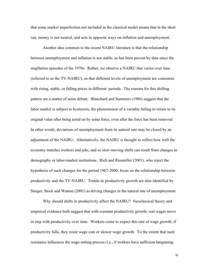
Why should shifts in productivity affect the NAIRU? Neoclassical theory and

empirical evidence both suggest that with constant productivity growth, real wages move

in step with productivity over time. Workers come to expect this rate of wage growth; if

productivity falls, they resist wage cuts or slower wage growth. To the extent that such

resistance influences the wage-setting process (i.e., if workers have sufficient bargaining

10

power), the resultant mismatch between productivity growth and real wage growth

worsens the inflation-unemployment tradeoff: the NAIRU rises4.

The U.S. economy suffered such a productivity shock in the Great Depression.

As depicted by figure 3, productivity growth trended downward through most of the

1920s and early 1930s, turning negative in 1932-3.5 This suggests a possible rise in the

NAIRU, as does figure 4, which presents a scatterplot of inflation and unemployment for

the years 1890-1942. Two trendlines are plotted; the trend for 1930-1942 intersects the

x-axis to the right of that for 1890-1929, suggesting that the level of unemployment

consistent with stable prices had risen by the 1930s. This, in turn, gives rise to the

possibility that actual unemployment, though high, may have been below the natural rate

of unemployment at times during the Depression and recovery period. If this were the

case, inflation during these times would not be a puzzle at all, but would merely be what

the standard Phillips curve predicts.

4. A TV-NA IRU Phillips Curve Model

To examine this question empirically, I turn to a Phillips curve model that allows

for time variation in the NAIRU. In particular, following Staiger, Stock and Watson

(2001), I generate forecasts of inflation from a model that explicitly captures the long-run

4 See Mankiw and Reis (2001b) for an interesting interpretation of the role of the slowdissemination of information in driving this process.5 Note that here and elsewhere, productivity is measured as trend productivity – calculated asa four-year moving average of Kendrick’s output per manhour in the nonfarm business sector– to avoid low frequency measurement error and cyclicality in the data.

11

relationship of real wage growth and productivity growth, and relates changes in the

NAIRU to deviations from that trend.

4.1 A Wage-Price Phillips Curve System

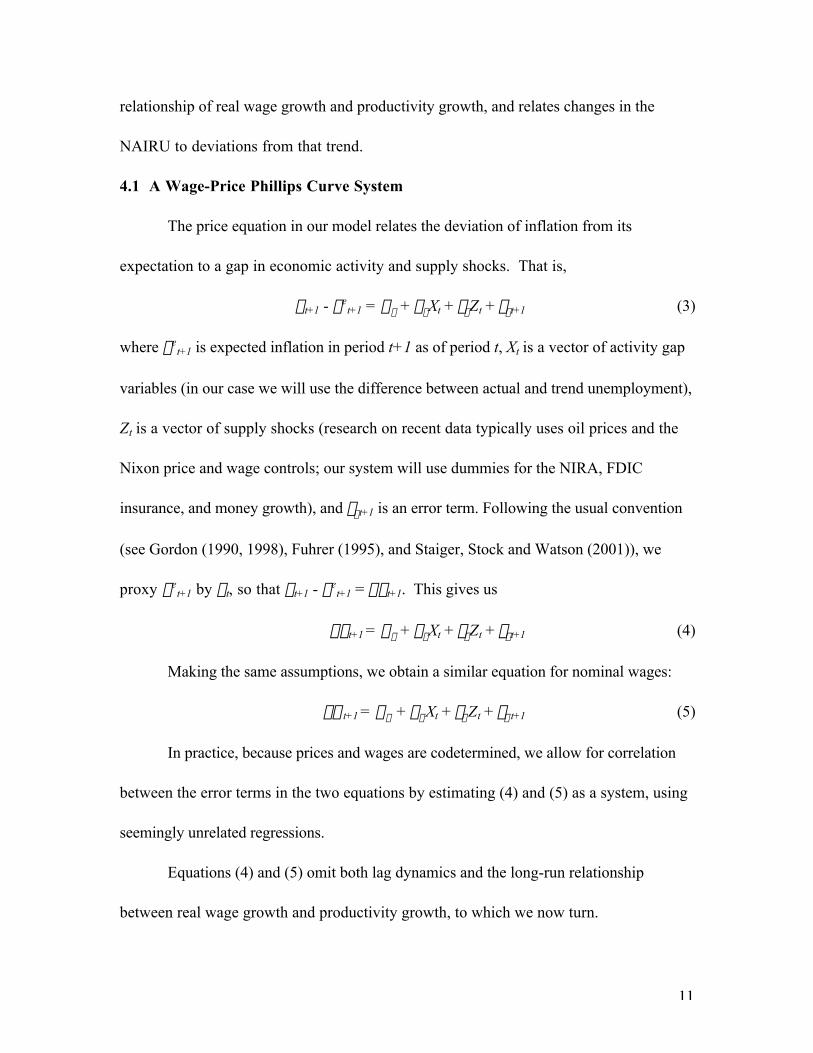
The price equation in our model relates the deviation of inflation from its

expectation to a gap in economic activity and supply shocks. That is,

pt+1 - pet+1 = ap + bpXt + gpZt + ept+1 (3)

where pet+1 is expected inflation in period t+1 as of period t, Xt is a vector of activity gap

variables (in our case we will use the difference between actual and trend unemployment),

Zt is a vector of supply shocks (research on recent data typically uses oil prices and the

Nixon price and wage controls; our system will use dummies for the NIRA, FDIC

insurance, and money growth), and ept+1 is an error term. Following the usual convention

(see Gordon (1990, 1998), Fuhrer (1995), and Staiger, Stock and Watson (2001)), we

proxy pet+1 by pt, so that pt+1 - p

et+1 = Dpt+1. This gives us

Dpt+1 = ap + bpXt + gpZt + ept+1 (4)

Making the same assumptions, we obtain a similar equation for nominal wages:

Dwt+1 = aw + bwXt + gwZt + ewt+1 (5)

In practice, because prices and wages are codetermined, we allow for correlation

between the error terms in the two equations by estimating (4) and (5) as a system, using

seemingly unrelated regressions.

Equations (4) and (5) omit both lag dynamics and the long-run relationship

between real wage growth and productivity growth, to which we now turn.

12

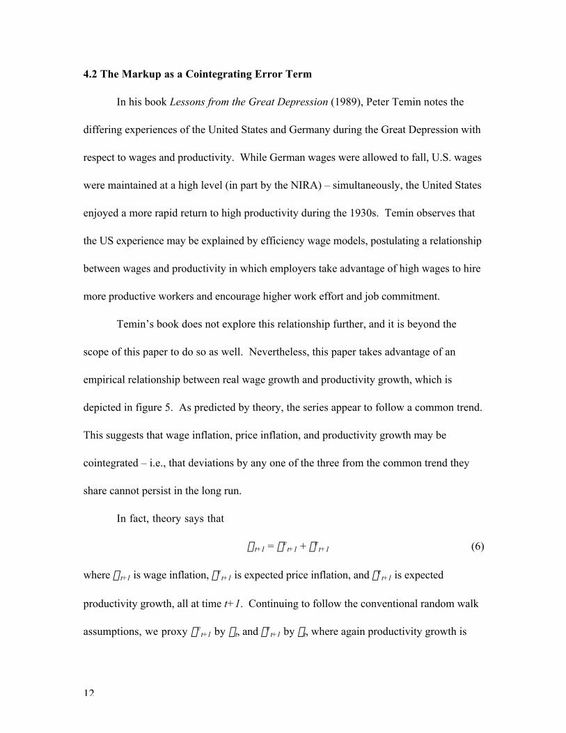
4.2 The Markup as a Cointegrating Error Term

In his book Lessons from the Great Depression (1989), Peter Temin notes the

differing experiences of the United States and Germany during the Great Depression with

respect to wages and productivity. While German wages were allowed to fall, U.S. wages

were maintained at a high level (in part by the NIRA) – simultaneously, the United States

enjoyed a more rapid return to high productivity during the 1930s. Temin observes that

the US experience may be explained by efficiency wage models, postulating a relationship

between wages and productivity in which employers take advantage of high wages to hire

more productive workers and encourage higher work effort and job commitment.

Temin’s book does not explore this relationship further, and it is beyond the

scope of this paper to do so as well. Nevertheless, this paper takes advantage of an

empirical relationship between real wage growth and productivity growth, which is

depicted in figure 5. As predicted by theory, the series appear to follow a common trend.

This suggests that wage inflation, price inflation, and productivity growth may be

cointegrated – i.e., that deviations by any one of the three from the common trend they

share cannot persist in the long run.

In fact, theory says that

wt+1 = pet+1 + qe

t+1 (6)

where wt+1 is wage inflation, pet+1 is expected price inflation, and qe

t+1 is expected

productivity growth, all at time t+1. Continuing to follow the conventional random walk

assumptions, we proxy pet+1 by pt, and qe

t+1 by qt, where again productivity growth is

13

measured as a four-year moving average. This leads to a specification of the cointegrating

relationship as

wt+1 = pt + qt (7)

In other words, if price inflation, wage inflation, and productivity growth are

integrated of order one (I(1)), then pt -wt+1 + qt, sometimes referred to as the markup,

should be stationary over time (integrated of order zero, or I(0)). Support for such an

empirical relationship can be found for the U.S. from 1960-2000 in Staiger, Stock and

Watson (2001) and Banerjee, Cockerell and Russell (2001) in Australian data from 1972

to 1995.

Tables 5.1 and 5.2 presents empirical tests of the univariate and multivariate

trends in the data. Inflation is calculated as the log difference of the implicit GNP

deflator; wage inflation is measured as the log difference in average hourly earnings in the

nonfarm business sector, which is in turn calculated as Lebergott’s average annual

nonfarm earnings series divided by Kendrick’s annual nonfarm manhour series. I use the

interwar (1919-1942) sample, and test current wage inflation, lagged price inflation, and

lagged productivity growth for unit roots, and the trivariate system for a cointegrating

relationship.

Augmented Dickey-Fuller unit root tests, assuming trends in the data, do not

reject the hypothesis of a unit root for any of the three series at the 10% significance

level. Using the same set of assumptions, a Johansen cointegration test finds evidence of

a single cointegrating relationship between the three. This evidence supports the

hypothesis that real wages, adjusted for productivity growth, are stationary: deviations

14

from the long-run trend shared by the three are not persistent; the markup, therefore, can

be used as an error-correction term in the sense of Granger (1983).

To make this clear, we augment our earlier wage-price system as follows:

Dpt+1 = ap + b1p(L)Dpt + b2p(L)(pt -wt+1 + qt,) + b3pXt + b4pZt + ept+1 (8.1)

Dwt+1 = aw + b1w(L)Dwt + b2w(L)( pt -wt+1 + qt,) + b3wXt + b4wZt + ewt+1 (8.2)

System (8) is referred to as the triangular representation of a system with

cointegrated variables. (pt -wt+1 + qt,) is referred to as an error-correction term because

deviations from its mean forecast adjustments in the cointegrated variables to reestablish

the long-run cointegrating trend. Assuming that the slope coefficients on the other

variables in system (8) are stable, the sum of the error-correction term and the constant

intercept term can be interpreted as a time-varying intercept for the system, any drift in

which reflects shifts in the NAIRU (cf. Staiger, Stock, and Watson (2001)).

The actual series values for the markup are constructed using the dynamic OLS

procedure of Stock and Watson (1999), in which lagged price inflation is regressed on

wage inflation and lagged productivity growth, as well as two leads and lags each of the

change in wage inflation and the change in lagged productivity growth. The coefficients

on wage inflation (gw) and lagged productivity growth (gq) are then used to construct the

markup: markupt = pt-1 -gwwt -gqqt-1.6 Table 5.3 presents an ADF unit root test for the

markup, which rejects the hypothesis of a unit root at the 1% significance level; a plot of

the markup (Figure 6) further supports the hypothesis that the markup is stationary.

6 Note that gq is negative, preserving the proper signs in the markup.

15

5. Results

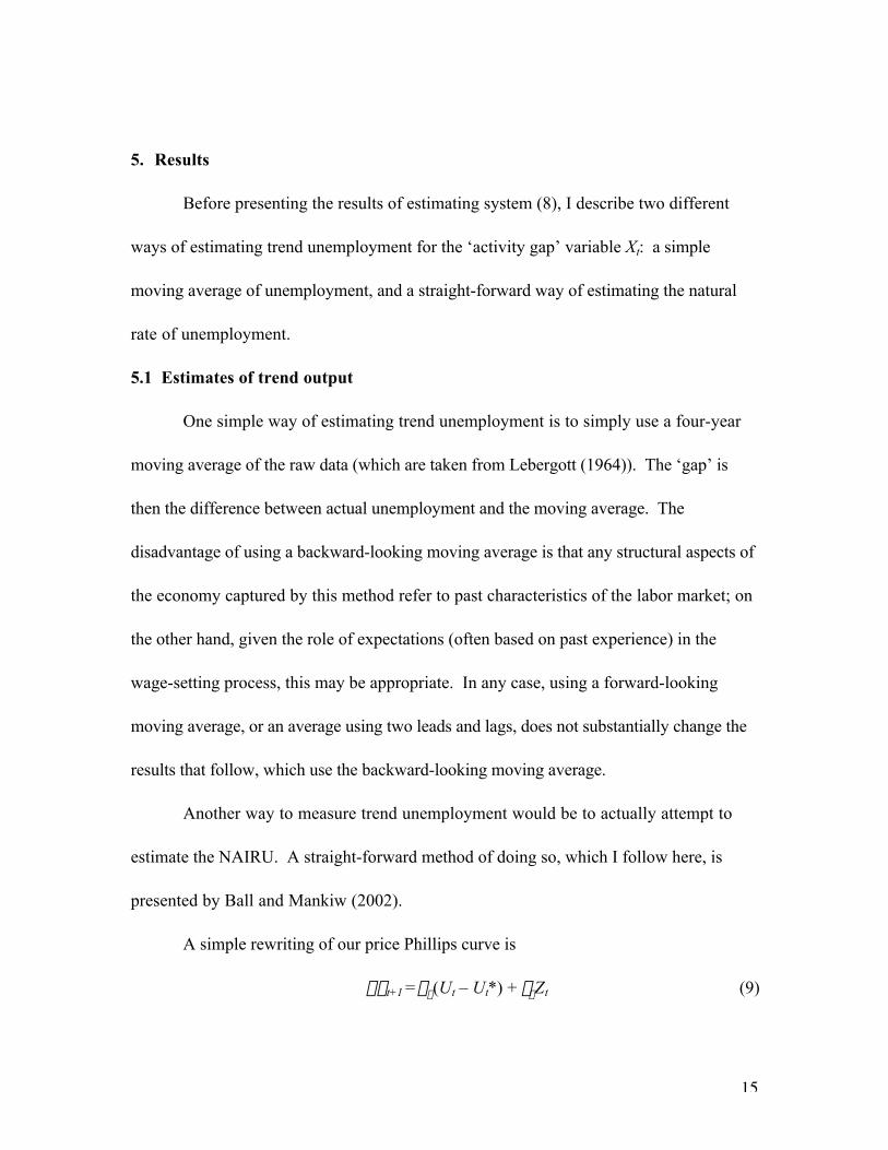
Before presenting the results of estimating system (8), I describe two different

ways of estimating trend unemployment for the ‘activity gap’ variable Xt: a simple

moving average of unemployment, and a straight-forward way of estimating the natural

rate of unemployment.

5.1 Estimates of trend output

One simple way of estimating trend unemployment is to simply use a four-year

moving average of the raw data (which are taken from Lebergott (1964)). The ‘gap’ is

then the difference between actual unemployment and the moving average. The

disadvantage of using a backward-looking moving average is that any structural aspects of

the economy captured by this method refer to past characteristics of the labor market; on

the other hand, given the role of expectations (often based on past experience) in the

wage-setting process, this may be appropriate. In any case, using a forward-looking

moving average, or an average using two leads and lags, does not substantially change the

results that follow, which use the backward-looking moving average.

Another way to measure trend unemployment would be to actually attempt to

estimate the NAIRU. A straight-forward method of doing so, which I follow here, is

presented by Ball and Mankiw (2002).

A simple rewriting of our price Phillips curve is

Dpt+1 =bp(Ut – Ut*) + gpZt (9)

16

where we have explicitly written our gap variable as unemployment (Ut) less the natural

rate of unemployment (Ut*). If it is assumed that the supply shocks are uncorrelated

with contemporaneous values of Ut, then this equation can be estimated by OLS. This, of

course, is a rather strong assumption: many supply shocks will, in fact, be correlated

with unemployment. While this problem could be handled by use of instrumental

variables which are correlated with the supply shocks but not with unemployment, in

practice finding such instruments is very difficult and rarely done.

Another econometric issue with estimating the NAIRU is that of standard errors.

Only recently has the literature attempted to put standard errors on estimates of the

NAIRU. Stock, Staiger and Watson (1997) estimated a NAIRU of 6.2 percent in 1990,

with a 95 percent confidence interval of 5.1 to 7.7 percent. Using a Kalman smoother

(which requires more data than is available for the Depression period), the same authors

narrow their error bands to ±0.4 percentage points in their 2001 paper, but in any case it

appears that given existing specifications, the NAIRU is not estimated precisely. In what

follows I present only point estimates.

A first pass at estimating the NAIRU might be undertaken by assuming that U* is

not a function of time, but is constant through the sample. Then we can rewrite (9) as

Dpt+1 =bpUt – bpU* + gpZt (10)

Now, if we regress the change in inflation on a constant, unemployment, and a vector of

supply shocks (I use the NIRA dummy, the FDIC dummy, and the growth rates of the

currency-deposit ratio, the loan-deposit ratio, and the level of bank loans), then the ratio

17

of the absolute value of the constant term (bpU*) to that of the coefficient on

unemployment (bp) gives an estimate of U*. When we do this using data from 1919 to

1942, we estimate a constant of –3.36, and a coefficient of -0.25 on unemployment,

leading to an estimate of 13.7 percent for the natural rate of unemployment.

Of course, as has already been emphasized, the NAIRU is not constant over time.

To estimate the path of a TV-NAIRU, rewrite equation (10) as

U* - gpZt/bp = Ut - Dpt+1/bp (11)

The right-hand side of this equation can be calculated from the data, where we use the

same bp (-0.25) as that estimated in equation (10). The left hand side, on the other hand,

is the difference between the NAIRU and a term proportional to the supply shocks. It is

often assumed in the literature that movements in the natural rate of unemployment are

long-term movements, reflecting relatively slow changes in the unemployment-inflation

tradeoff; higher frequency fluctuations in the right hand side of (11) can therefore be

attributed to the shorter-term supply shocks. This leads to the estimation of the NAIRU

as the trend component of the right-hand side of equation (11).

I use the Hodrick-Prescott Filter to attain the trend component of the data

(Hodrick and Prescott (1997)). The HP Filter minimizes the sum of squared deviations

between a linear time trend and the actual data, with a penalty for curvature to smooth the

trend. The higher the penalty, the smoother the estimated trend; I use a penalty

parameter value of 100, which is the most common value used with annual data.

18

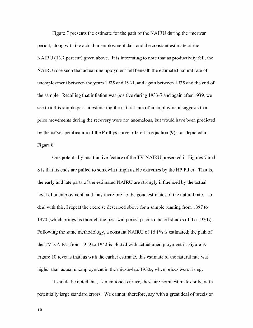
Figure 7 presents the estimate for the path of the NAIRU during the interwar

period, along with the actual unemployment data and the constant estimate of the

NAIRU (13.7 percent) given above. It is interesting to note that as productivity fell, the

NAIRU rose such that actual unemployment fell beneath the estimated natural rate of

unemployment between the years 1925 and 1931, and again between 1935 and the end of

the sample. Recalling that inflation was positive during 1933-7 and again after 1939, we

see that this simple pass at estimating the natural rate of unemployment suggests that

price movements during the recovery were not anomalous, but would have been predicted

by the naïve specification of the Phillips curve offered in equation (9) – as depicted in

Figure 8.

One potentially unattractive feature of the TV-NAIRU presented in Figures 7 and

8 is that its ends are pulled to somewhat implausible extremes by the HP Filter. That is,

the early and late parts of the estimated NAIRU are strongly influenced by the actual

level of unemployment, and may therefore not be good estimates of the natural rate. To

deal with this, I repeat the exercise described above for a sample running from 1897 to

1970 (which brings us through the post-war period prior to the oil shocks of the 1970s).

Following the same methodology, a constant NAIRU of 16.1% is estimated; the path of

the TV-NAIRU from 1919 to 1942 is plotted with actual unemployment in Figure 9.

Figure 10 reveals that, as with the earlier estimate, this estimate of the natural rate was

higher than actual unemployment in the mid-to-late 1930s, when prices were rising.

It should be noted that, as mentioned earlier, these are point estimates only, with

potentially large standard errors. We cannot, therefore, say with a great deal of precision

19

that actual unemployment was below the NAIRU. We do, nevertheless, observe that the

path of the NAIRU appears to have been trending upwards into the mid-1930s, when

prices began to rise, such that the gap between unemployment and its trend was surely

shrinking, lessening the mystery surrounding recovery-period inflation.

I turn now to the results of estimating system (8), using each of our three

measures of trend unemployment in turn.

5.2 Results from the Price-Wage Phillips Curve System

I estimate system (8) using three measures of trend output to construct my ‘gap’

variable: the simple four-year moving average of unemployment, and the two estimated

paths of the TV-NAIRU discussed in the previous section. Estimation output for the

two specifications is presented in Table 6. There is a noticeable improvement in fit (as

measured by adjusted R-squared) in the model using the TV-NAIRU estimated over

1919-42, although the effect is less using the TV-NAIRU estimated over 1897-1970.

However, it is interesting to note the differences between the coefficients on the gap

variable and on the error-correction term in the two models. Using the difference between

actual unemployment and the 1919-42 TV-NAIRU as the gap, the error-correction term

becomes much more significant and takes on the correct signs (recall that the markup is

calculated as pt-1 -gwwt -gqqt; if it is high, then inflation is above trend, which implies that

inflation should fall to adjust back to trend in the next period), while the coefficients on

the gap variable become less significant. This is consistent with the hypothesis that

deviations from the long-run trend shared by real wage growth and productivity growth

20

are associated with changes in the NAIRU; information contained in the gap between

unemployment and the TV-NAIRU is captured by the markup.7

Fitted values for inflation generated by the estimation are provided for the years

1933-42 in Figure 11. The models fit the data quite well; the root mean square error of

the fitted values using the four-year moving average as trend unemployment is 0.0413;

using the TV-NAIRU estimated over 1919-42, the RMSE is 0.0205; using the TV-

NAIRU estimated over 1897-1970, the RMSE is 0.0416. The models correctly predict

the direction of movements in the price level for nearly all years, without explicitly

incorporating growth rate effects into the model (I do, of course, include a dummy for the

NIRA as one of my supply shock controls).

To sum up the findings of the previous two sections: price inflation, wage

inflation, and productivity growth follow a common trend; deviations from this trend

constitute a time-varying intercept term closely related to the TV-NAIRU in a price-wage

Phillips curve system (it is interesting to note the coincidence of the peak in the estimated

NAIRUs and the trough of trend productivity growth, depicted in Figures 12 and 13).

Estimates of the path of the TV-NAIRU during the Depression and recovery period

suggest that the drop in productivity pushed the TV-NAIRU up such that actual

unemployment fell below its natural rate at roughly the same time that prices rose, just as

predicted by the standard Phillips curve model of the inflation-unemployment tradeoff.

7 Staiger, Stock and Watson (2001) actually use the markup to estimate the TV-NAIRU as atime-varying intercept term in the Phillips curve system. However, doing so requiresimplementation of the Kalman filter, for which more observations are required than areavailable for the interwar period.

21

Using a model of this tradeoff which explicitly takes account of the role of the long-run

relationship between productivity growth and real wage growth, the direction of price

movements during the recovery period is correctly predicted for nearly all years from

1933-42.

Thus, the fall in productivity of the late 1920s and early 1930s implied a rise in

the NAIRU which all but removes the puzzle of inflation during the 1930s: price rises

were simply a consequence of the usual Phillips-curve relationship, albeit one in which

the rate of unemployment consistent with stable prices had risen to levels much higher

than in past years. What remains to be explained is the source of that fall in productivity.

One possibility is that the period coincided with large-scale destruction of productivity-

enhancing technology. This does not seem to be the case, however; not only were

technologies not lost, but Field (1999) finds evidence that the period from 1929-1941 was

the most technologically progressive in U.S. history. Indeed, the late 1930s saw

productivity growth return to positive territory as new technologies were implemented.

It must be, then, that during the Depression and in the early recovery years, something

was preventing new and existing technologies from being applied, projects which could

have benefited from them being undertaken, investments from being made. In what

follows, I argue that the tightening of financial conditions and the destruction of financial

intermediary capacity, in both the U.S. and global economy, were significant factors in

explaining the productivity decline.

22

6. The Effects of the Financial Crisis on Productivity During the Depression

In their classic work A Monetary History of the United States, 1867-1960 (1963),

Milton Friedman and Anna Schwartz portray the Great Depression as a time of

numerous bank failures, bank runs, a rise in the currency-deposit and reserve-deposit

ratio, and falls in the level of bank loans, the ratio of loans to securities in bank portfolios,

and the loan-deposit ratio (some of these data are plotted in Figures 14-16). In other

words, it was a time of severe financial tightening, caused by catastrophic turmoil in the

capital markets (the specific reasons for this chaos, ranging from the bursting of a stock

market bubble in 1929 to international politics to dogmatic adherence to the gold standard,

are beyond the scope of this paper; see Bernanke (1995), Bordo (1997), Calomiris and

Hubbard (1996), Field (1992), Friedman and Schwartz (1963), Hart (1938), Obstfeld and

Taylor (2002), and Temin (1989) for various explanations). Numerous authors have

emphasized a link from financial conditions to macroeconomic performance. Fisher

(1933) and Hart (1938) speak of the role of inside debt; Mishkin (1978) and Hubbard

(1995) focus on household balance sheets, liquidity, and the so-called ‘credit channel’.

Friedman (1981) writes of the link between credit and aggregate activity. The classical

story told of the link from the financial sector to the macroeconomy is that offered by

Friedman and Schwartz (1963), who stressed the effects of the banking crisis on the

money supply.

In theory, however, money can only impact the real economy in the short run, as

mentioned earlier. Due to the lack of theoretical grounding for persistent nonneutrality of

money, which would have to be present to support a purely monetary link from capital

23

markets to the real economy, a different story has been told by Bernanke (1983) and

Bernanke and Gertler (1989, 1990). Here the focus is on agency costs and market

imperfections, especially asymmetric information between lenders and borrowers, which

give rise to a demand for financial intermediation. The cost of credit intermediation is

particularly emphasized; the CCI is defined as being ‘the cost of channeling funds from

the ultimate savers/lenders into the hands of good borrowers… (including) screening,

monitoring, and accounting costs, as well as the expected losses inflicted by bad

borrowers.’ (Bernanke (1983), p. 263) While no direct measure or the CCI exists,

Bernanke (1983) presents data similar to that plotted in Figures 14-16, illustrative of a

rise in the CCI caused by the financial crisis. A vicious feedback loop from the CCI to

defaults and bankruptcies developed (the financial crisis pushed many firms into

bankruptcy, which made banks more hesitant to extend credit, which forced more

borrowers to default or declare bankruptcy, etc.), greatly reducing the efficacy of the

financial intermediation infrastructure.

A useful survey of the literature on the link between financial intermediation and

the macroeconomy is provided by Hubbard (1997). A point of consensus through this

literature is the importance of financial intermediation for productivity in the complex

U.S. economy, bringing together borrowers and investors in a deep, relatively anonymous

market for capital. Cooper and Ejarque (1995) point out the possibility of multiple

investment and productivity equilibria, depending on the efficiency of financial

intermediation. As capital markets grow less efficient, they argue, individuals substitute

from future to current consumption to avoid investing in a period of high costs and low

24

expected returns. A similar argument is common to much of the literature. Gertler (1988)

shows that beliefs regarding future economic conditions can affect the CCI (because, for

instance, borrowers may offer claims on future earnings as collateral); higher CCI, in turn,

can adversely affect current capacity utilization. Calomiris, Himmelberg, and Wachtel

(1994), Kashyap, Stein and Lamont (1994), and Kashyap, Stein and Wilcox (1993) all

argue that in times of inefficient financial intermediation, firms with poor balance sheets

will choose to build up ‘buffer stocks’ of capital and cash to improve their net asset

position, resulting in a drop in investment and activity. According to Greenwald and

Stiglitz (1989), failures in equity markets curtail the abilities of firms to diversify the risks

of their investments and operations.

What all of these arguments point to (and as is explicitly argued by Gertler (1988)

and Greenwald and Stiglitz (1989)) is that financial crisis, by raising the CCI, can severely

limit investment, activity, on-the-job training, learning-by-doing, information spillovers,

and research and development: all crucial components of productivity growth. Given the

severity of the financial crisis and the fall in productivity leading into the Depression, it

seems likely that this is precisely what drove the rise in the natural rate of unemployment

in the late 1920s and early 1930s. The crucial point is that trend output is not merely a

multiple of the stocks of capital and labor in the economy. Intangible capital, such as

financial intermediation, plays an important role in determining the productive capacity of

the U.S. economy (cf. Williamson (1989)), and of the international economy as well (see

Bernanke (1995), Bernanke and James (1991) and Obstfeld and Taylor (2002)). It was

not lack of physical capital, but lack of confidence in the system of financial

25

intermediation so necessary to put that capital to use, that curtailed productivity growth

and drove potential output down during the Great Depression. This, in turn, translated

into a rise in the natural rate of unemployment, making the price rises of the 1930s

possible.

7. Conclusion

This paper has argued that financial crisis during the Great Depression raised the

costs of credit intermediation and severely hindered the growth of productivity in the

United States economy. The fall in productivity worsened the unemployment-inflation

tradeoff, causing the natural rate of unemployment to rise to the point that actual

unemployment, though high throughout much of the recovery, may actually have fallen

below the NAIRU in certain years (crucial to this finding was the identification of the

long-run trend shared by real wage growth and productivity growth, and the role that

deviations from this trend play in shifting the TV-NAIRU). Inflation followed: in effect,

though the physical capital stock had not fallen greatly, sufficient intangible (i.e.,

financial) capital had been destroyed that the economy was straining against the bounds

of its potential. It is beyond doubt that the rapid growth rate of the economy played a

significant role in this process; nevertheless, the growth rate need not be invoked to

explain inflation in the 1930s. That prices rose was not a puzzle: it was simply the

ordinary workings of the relationship between unemployment and inflation described by

the standard Phillips curve.

26

The exact link between financial crisis and productivity has only been sketched

here. This paper did not attempt a formal modeling of this relationship beyond those

provided by the past literature cited above. However, none of these papers attempts

such a model specifically for the events of the Great Depression: this, then, is an area for

future research. An additional question not addressed in this paper is the causality, if

any, which characterizes the relationship between real wage growth and productivity

growth. As noted above, the US and Germany followed essentially opposite paths in

both these areas during the recovery: the US set high wages and enjoyed high

productivity, while Germany restricted wage growth and stagnated. It is an unsettled

question whether there is a direct link between wages and productivity, beyond the

merely empirical relationship used in this paper. Productivity is arguably the most

important variable for any economy; this question, then, is one that deserves great

attention.

Table 1Macroeconomic Indicators for 1933-42

Inflation Rate (Implicit GNP Deflator)

Real GNP (Millions of

1996$)

Trend GNP (Millions of

1996$)

Deviation from Trend GNP

Real GNP Growth Unemployment Rate

Inflation Rate (Raw Materials Prices)

Inflation Rate (All Commodites Prices)

1933 -2.6% 606.42 927.71 -42.5% -1.7% 24.9% 2.5% 1.7%1934 5.4% 671.73 957.84 -35.5% 10.2% 21.7% 19.4% 12.8%1935 1.9% 732.60 988.95 -30.0% 8.7% 20.1% 11.7% 6.6%1936 1.2% 825.15 1021.06 -21.3% 11.9% 16.9% 3.6% 1.0%1937 4.1% 869.93 1054.22 -19.2% 5.3% 14.3% 6.0% 6.6%1938 -3.1% 840.62 1088.46 -25.8% -3.4% 19.0% -16.4% -9.3%1939 -1.1% 908.64 1123.81 -21.3% 7.8% 17.2% -2.5% -1.9%1940 1.5% 984.51 1160.30 -16.4% 8.0% 14.6% 2.4% 1.9%1941 6.5% 1154.26 1197.98 -3.7% 15.9% 9.9% 15.0% 10.5%1942 7.6% 1364.17 1236.89 9.8% 16.7% 4.7% 18.6% 12.4%

Mean 2.1% 895.80 1075.72 -20.6% 7.9% 16.3% 6.0% 4.2%Standard Deviation 3.7% 226.94 103.99 15.1% 6.6% 5.9% 10.8% 6.9%

Notes: Trend GNP is calculated by extending forward the average growth rate of real GNP from 1910-24. Inflation rates are calculated aslog differences, as is the deviation of real GNP from trend GNP. Sources are in the Data Appendix.

Table 2Forecasts of Inflation from Romer (1999)

Actual InflationForecast Using Base

Phillips CurveForecast Including

Growth Rate Effects

Fitted Values Including Growth Rate Effects and

NIRA

Fitted Values Including Growth Rate Effects but

not NIRA

1933 -2.6% -14.1% -11.9% -0.4% -7.7%1934 5.4% -13.0% -5.4% 8.0% 1.4%1935 1.9% -11.4% -3.2% 4.3% 1.9%1936 1.2% -8.1% 2.3% 3.4% 5.0%1937 4.1% -7.2% -1.3% -0.7% 1.2%1938 -3.1% -9.5% -8.8% -7.4% -5.0%1939 -1.1% -8.3% -1.9% -1.0% 1.5%1940 1.5% -6.8% 0.0% 0.5% 2.9%1941 6.5% -2.6% 8.1% 7.4% 9.5%1942 7.6% 2.1% 12.7% 11.1% 12.1%

Notes: All inflation rates refer to the implicit GNP deflator. Forecasts are reproduced from Romer (1999), with the exception ofcolumn 5, which are the author's calculations. Other sources are in the Data Appendix.

Table 3Average Real GNP Growth Between Benchmark Dates

Period Average Real GNP Growth1873-1883 4.81%1884-1889 2.64%1890-1899 3.68%1900-1909 3.70%1910-1923 3.25%1924-1941 2.98%1942-1952 4.53%1953-1964 3.43%1965-1977 3.56%1978-1985 2.91%1986-1995 2.74%1996-2001 3.33%

27

Table 4Model Stability Tests

(Unemployment - Four-year Moving Average) = a + b(Deviation from Trend GNP)

Chow Breakpoint Test: 1924F-statistic 4.207 Probability 0.021Log Likelihood Ratio 8.398 Probability 0.015

Chow Forecast Test: Forecast from 1924 to 1942F-statistic 2.594 Probability 0.010Log Likelihood Ratio 49.652 Probability 0.000

Notes: The Model is estimated over the sample period 1893 to 1942. Sourcesare in the Data Appendix

Table 5 Unit Root and Cointegration Tests

Table 5.1 - Unit Root Tests for Price Inflation, Wage Inflation, and Trend Productivity Growth

VariableADF Test Statistic

10% Critical Value

5% Critical Value

1% Critical Value

p t-1 -2.802695 -3.2418 -3.6118 -4.3942

w t -3.134428 -3.2418 -3.6118 -4.3942

q t-1 -2.671466 -3.2418 -3.6118 -4.3942

Table 5.2 - Johansen Cointegration Test for the Trivariate System

Hypothesized Number of Cointegrating Relationships

Eigenvalue Likelihood Ratio

5% Critical Value

1% Critical Value

None** 0.755305 54.54354 42.44 48.45At Most One 0.526688 20.7577 25.32 30.45At Most Two 0.110328 2.805669 12.25 16.26

Table 5.3 - Unit Root Test for the Markup

VariableADF Test Statistic

10% Critical Value

5% Critical Value

1% Critical Value

p t-1 - g w w t - g q q t-1 -4.52** -3.2535 -3.633 -4.4418

Notes: All tests are performed over the sample 1919 to 1942. The tests allow for a linear deterministic trend in the data. *(**) indicates rejection of the given hypothesis at the5%(1%) significance level. Price inflation and trend productivity growth are laggedvalues to conform with theory, which says that wage inflation should equal expectedprice inflation plus expected productivity growth. Sources are in the Data Appendix.

28

Table 6Estimation Output for Price-Wage Phillips Curve Systems

Using Four-Year Moving Average as Trend Unemployment

Using NAIRU Estimated over 1919-42 as Trend Unemployment

Using NAIRU Estimated over 1897-1970 as Trend Unemployment

Change in Price Inflation Change in Price Inflation Change in Price InflationConstant 0.02 (0.03) Constant -0.08** (0.03) Constant -0.04 (0.06)

Markup(-1) 0.21 (0.35) Markup(-1) -0.34 (0.27) Markup(-1) -0.09 (0.67)Markup(-2) -0.33 (0.25) Markup(-2) -0.47** (0.15) Markup(-2) -0.25 (0.40)(U-U*)(-1) -2.55** (0.71) (U-U*)(-1) 0.18 (0.57) (U-U*)(-1) -1.74 (1.36)(U-U*)(-2) 0.68 (0.60) (U-U*)(-2) -0.09 (0.40) (U-U*)(-2) 1.85* (0.86)

M2 Growth Rate(-1)

-0.50 (0.33) M2 Growth Rate(-1)

0.65* (0.27) M2 Growth Rate(-1)

-0.28 (0.52)

M2 Growth Rate(-2)

-0.51 (0.28) M2 Growth Rate(-2)

0.39* (0.15) M2 Growth Rate(-2)

-0.20 (0.23)

NIRA 0.08 (0.11) NIRA 0.30** (0.09) NIRA 0.03 (0.19)FDIC 0.02 (0.03) FDIC -0.01 (0.02) FDIC 0.06 (0.03)

Change in Price Inflation(-1)

-0.99* (0.40) Change in Price Inflation(-1)

-0.60 (0.37) Change in Price Inflation(-1)

-1.03 (0.88)

Change in Price Inflation(-2)

-0.61* (0.22) Change in Price Inflation(-2)

-0.707193 (0.13) Change in Price Inflation(-2)

-0.37 (0.32)

R-squared 0.733 0.795 0.675 Adjusted R-squared 0.490 0.591 0.380

Change in Wage Inflation Change in Wage Inflation Change in Wage InflationConstant 0.04* (0.02) Constant 0.02 (0.02) Constant -0.01 (0.02)

Markup(-1) 1.89** (0.60) Markup(-1) 0.83 (0.55) Markup(-1) 0.77 (0.66)Markup(-2) -0.81 (0.60) Markup(-2) -0.33 (0.42) Markup(-2) -0.65 (0.45)(U-U*)(-1) -0.36 (0.75) (U-U*)(-1) -0.04 (0.75) (U-U*)(-1) -1.72* (0.75)(U-U*)(-2) -0.06 (0.60) (U-U*)(-2) -0.15 (0.59) (U-U*)(-2) 1.02 (0.59)

NIRA 0.05 (0.07) NIRA -0.04 (0.06) NIRA 0.06 (0.04)Change in Price

Inflation(-1)0.39 (0.35) Change in Price

Inflation(-1)0.69 (0.37) Change in Price

Inflation(-1)-0.05 (0.32)

Change in Price Inflation(-2)

-1.46 (0.81) Change in Price Inflation(-2)

-0.44 (0.61) Change in Price Inflation(-2)

-0.85 (0.61)

Change in Wage Inflation(-1)

0.97 (0.68) Change in Wage Inflation(-1)

-0.06 (0.56) Change in Wage Inflation(-1)

0.24 (0.58)

Change in Wage Inflation(-2)

-0.18 (0.23) Change in Wage Inflation(-2)

-0.29 (0.20) Change in Wage Inflation(-2)

-0.18 (0.18)

R-squared 0.734 0.818 0.785 Adjusted R-squared 0.534 0.669 0.624

Notes: Estimation is by seemingly unrelated regressions of the price-wage Phillips curve system (System (8) in the text). *(**) indicatessignificance at the 5%(1%) level. Sources are in the Data Appendix.

29

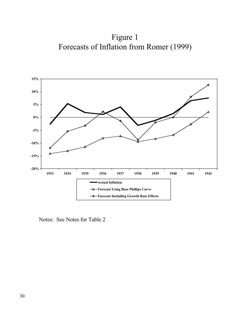
Figure 1Forecasts of Inflation from Romer (1999)

-20%

-15%

-10%

-5%

0%

5%

10%

15%

1933 1934 1935 1936 1937 1938 1939 1940 1941 1942

Actual Inflation

Forecast Using Base Phillips Curve

Forecast Including Growth Rate Effects

Notes: See Notes for Table 2

30

Figure 2Two Measures Of Trend Output

-50%

-40%

-30%

-20%

-10%

0%

10%

20%

1893 1900 1907 1914 1921 1928 1935 1942-50%

-40%

-30%

-20%

-10%

0%

10%

20%

Notes: Deviation from Trend Output is from Romer (1999); Unemployment– Four-Year Moving Average is actual unemployment minus a backward-looking four-year moving average of unemployment, and is plotted on aninverse scale. Sources are in the Data Appendix.

Deviation from Trend Output

Unemployment – Four-Year Moving Average

31

Figure 3Trend Productivity Growth

-3%

-2%

-1%

0%

1%

2%

3%

4%

5%

6%

7%

8%

1919 1921 1923 1925 1927 1929 1931 1933 1935 1937 1939 1941

-3%

-2%

-1%

0%

1%

2%

3%

4%

5%

6%

7%

8%

Notes: Trend Productivity Growth is calculated as a four-year backward-looking moving average of the log difference of productivity. Sources are inthe Data Appendix.

32

-10

-5

0

5

10

15

20

-20 -10 0 10 20 30 401930-1942

-10

-5

0

5

10

15

20

-20 -10 0 10 20 30 40

1890-1929

Figure 4Unemployment and Inflation, 1890-1942

Inflation (Percent)

Unemployment(Percent)

Notes: Sources are in the Data Appendix.

33

Figure 5Real Wage Growth and Trend Productivity Growth

-10%

-5%

0%

5%

10%

15%

20%

1919 1921 1923 1925 1927 1929 1931 1933 1935 1937 1939 1941

-10%

-5%

0%

5%

10%

15%

20%

Notes: Trend Productivity Growth is calculated as a four-year backward-looking moving average of the log difference of productivity. Real WageGrowth is calculated as wage inflation less price inflation. Sources are in theData Appendix.

Real Wage Growth

Trend Productivity Growth

34

Figure 6The Markup

-20%

-15%

-10%

-5%

0%

5%

10%

1919 1921 1923 1925 1927 1929 1931 1933 1935 1937 1939 1941

-20%

-15%

-10%

-5%

0%

5%

10%

Notes: The markup is calculated as pt-1 -gwwt -gqqt-1. See text for details.Sources are in the Data Appendix.

35

Figure 7The NAIRU: Estimation Sample 1919-1942

-20%

-10%

0%

10%

20%

30%

1919 1921 1923 1925 1927 1929 1931 1933 1935 1937 1939 1941

-20%

-10%

0%

10%

20%

30%

Notes: See text for estimation methods. Sources are in the Data Appendix.

Actual Unemployment

Time-Varying NAIRU

Constant NAIRU = 13.7%

Figure 8The NAIRU (Estimation Sample 1919-1942) and Inflation

-20%

-10%

0%

10%

20%

30%

1919 1921 1923 1925 1927 1929 1931 1933 1935 1937 1939 1941

-20%

-10%

0%

10%

20%

30%

Actual Unemployment

Time-Varying NAIRUInflation

36

Figure 9The NAIRU: Estimation Sample 1897-1970

-20%

-10%

0%

10%

20%

30%

1919 1921 1923 1925 1927 1929 1931 1933 1935 1937 1939 1941

-20%

-10%

0%

10%

20%

30%

Notes: See text for estimation methods. Sources are in the Data Appendix.

Actual Unemployment

Time-Varying NAIRU

Constant NAIRU = 16.1%

Figure 10The NAIRU (Estimation Sample 1897-1970) and Inflation

-20%

-10%

0%

10%

20%

30%

1919 1921 1923 1925 1927 1929 1931 1933 1935 1937 1939 1941

-20%

-10%

0%

10%

20%

30%

Actual Unemployment

Time-Varying NAIRUInflation

37

Figure 11Fitted Values for Inflation from the Price-Wage

Phillips Curve System

-20%

-15%

-10%

-5%

0%

5%

10%

15%

1919 1921 1923 1925 1927 1929 1931 1933 1935 1937 1939 1941-20%

-15%

-10%

-5%

0%

5%

10%

15%

4-yr MA NAIRU(1919-1942)NAIRU(1897-1970 Actual Inflation

Notes: ‘4-yr MA’ depicts the fitted values generated by the price-wagePhillips curve system using the four-year moving average of unemploymentas trend unemployment. ‘NAIRU(1919-1942’) uses the NAIRU estimatedover 1919-1942 as trend unemployment. ‘NAIRU(1897-1970’) uses theNAIRU estimated over 1897-1970 as trend unemployment. Sources are inthe Data Appendix.

38

-20%

-10%

0%

10%

20%

30%

1919 1921 1923 1925 1927 1929 1931 1933 1935 1937 1939 1941

-3%

-1%

1%

3%

5%

7%

9%

Notes: See text for estimation methods. Trend Productivity Growth iscalculated as a four-year backward-looking moving average of the logdifference of productivity. Sources are in the Data Appendix.

Time-Varying NAIRU

Figure 12The NAIRU (Estimation Sample 1919-1942) and Productivity

Growth

Trend Productivity Growth

-20%

-10%

0%

10%

20%

30%

1919 1921 1923 1925 1927 1929 1931 1933 1935 1937 1939 1941

-3%

-1%

1%

3%

5%

7%

9%

Time-Varying NAIRU

Figure 13The NAIRU (Estimation Sample 1897-1970) and Productivity

Growth

Trend Productivity Growth

39

Figure 14Currency/Deposit Ratio

6%

8%

10%

12%

14%

16%

18%

1919 1921 1923 1925 1927 1929 1931 1933 1935 1937 1939 1941

6%

8%

10%

12%

14%

16%

18%

Notes: Sources are in the Data Appendix.

Figure 15Bank Loans (Millions of Dollars)

10

15

20

25

30

35

40

1919 1921 1923 1925 1927 1929 1931 1933 1935 1937 1939 1941

10

15

20

25

30

35

40

Figure 16Bank Loans/Deposits Ratio

20%

30%

40%

50%

60%

70%

80%

1919 1921 1923 1925 1927 1929 1931 1933 1935 1937 1939 1941

20%

30%

40%

50%

60%

70%

80%

40

41

Data Appendix

BANK LOANS: Loans are for all banks, excluding those unincorporated or ‘private’banks not reporting to State banking authorities. Banks in US possessions are excludedexcept one national bank in Alaska, which was a member of the Federal Reserve Systemfrom the time it opened for business in April 1915 until it was placed in voluntaryliquidation in April 1921 and which in June 1919 had total deposits of $351,000.

Source: Banking and Monetary Statistics, Board of Governors of the Federal ReserveSystem (1943)

COMMODITY PRICE INFLATION: Commodity Price Inflation is the growth rate ofthe wholesale price index for all commodities.

Source: Romer (1999)

CURRENCY: Currency is calculated as annual averages of estimates of currency heldby the public by Milton Friedman and Anna Schwartz.

Source: Friedman and Schwartz (1963)

CONSUMER PRICE INFLATION: Inflation is calculated as the log difference of theimplicit GNP deflator.

Source: Romer (1999), Bureau of Economic Analysis

DEPOSITS: Deposits are total deposits at all banks, as defined in the note for bank loansabove.

Source: Banking and Monetary Statistics, Board of Governors of the Federal ReserveSystem (1943)

PRODUCTIVITY: Productivity is output per manhour in the nonfarm business sector.Trend Productivity is calculated as a four-year backward-looking moving average ofactual productivity. Trend Productivity Growth is calculated as log(productivityt) –log(productivityt-4).

Source: Kendrick (1961)

RAW MATERIALS INFLATION: Raw Materials Inflation is the growth rate of thewholesale price index for raw materials.

Source: Romer (1999)

REAL GNP: Real GNP is calculated as nominal GNP, divided by the implicit GNPdeflator, in $1996. Real GNP growth is the log difference of Real GNP.

42

Source: Romer (1999), Bureau of Economic Analysis

TREND GNP: Trend GNP is calculated as a piecewise linear trend, taking the mean ofreal GNP growth between the benchmark dates of 1873, 1884, 1890, 1900, 1910, 1924,1942, 1953, 1965, 1978, 1986, 1996, and 2001. Methodology based on Romer (1999)

Source: Romer (1999), Bureau of Economic Analysis

UNEMPLOYMENT: Unemployment data are measured as annual averages of monthlyfigures for the nonfarm business labor force. Trend unemployment is calculated as afour-year backward-looking moving average of actual unemployment, as well as twoestimates for the path of the time-varying NAIRU (see text for estimation methods).

Source: Lebergott (1964), Bureau of Labor Statistics

WAGE INFLATION: Wages are calculated as Lebergott’s average annual nonfarmearnings series divided by Kendrick’s annual nonfarm manhour series. Wage inflation isthe log difference of wages.

Source: Lebergott (1964), Kendrick (1961)

43

References

Akerlof, George and Janet Yellen. 1985. ‘A near-rational model of the business cycle,with wage and price inertia.’ Quarterly Journal of Economics 100(5,Supplement): 823-38.

Ball, Laurence and N. Gregory Mankiw. 2002. ‘The NAIRU in theory and practice.’Journal of Economic Perspectives 16(4): 115-36.

Ball, Laurence and David Romer. 1990. ‘Real rigidities and the nonneutrality ofmoney.’ Review of Economics Studies 57(April): 539-52.

Banerjee, Anindya, Lynne Cockerell and Bill Russell. 2001. ‘An I(2) analysis ofinflation and the markup.’ Journal of Applied Econometrics 16: 221-40.

Bernanke, Ben. 1983. ‘Nonmonetary effects of the financial crisis in the propogation ofthe Great Depression.’ American Economic Review 73(3): 257-76.

. 1995. ‘The macroeconomics of the Great Depression: a comparativeapproach.’ Journal of Money, Credit and Banking 27: 1-28.

Bernanke, Ben and Mark Gertler. 1989. ‘Agency costs, net worth, and businessfluctuations.’ American Economic Review 79(1): 14-31.

. 1990. ‘Financial fragility and economic performance.’ AmericanEconomic Review 80(1): 87-114.

Bernanke, Ben and H. James. 1991. ‘The gold standard, deflation and financial crisis inthe Great Depression: an international comparison.’ in Hubbard, R. Glenn, ed.,Financial Markets and Financial Crises. Chicago: University of Chicago Press.

Blanchard, Olivier and Nobuhiro Kiyotaki. 1987. ‘Monopolistic competition and theeffects of aggregate demand.’ American Economic Review 77(September): 647-66.

Blanchard, Olivier and Lawrence Summers. 1986. ‘Hysteresis and the Europeanunemployment problem.’ pp. 15-78 in S. Fischer, ed., NBER MacroeconomicsAnnual. Cambridge, Massachusetts: The MIT Press.

Board of Governors of the Federal System. 1943. Banking and Monetary Statistics.Washington, D.C.: The National Capital Press.

Bordo, Michael. 1997. ‘The gold standard as a good housekeeping seal of approval.’Journal of Economic History 56: 389-428.

44

Calomiris, Charles, Charles Himmelberg and Paul Wachtel. 1994. ‘Commercial paper,corporate finance, and the business cycle: a macroeconomic perspective.’ NBERWorking Paper No. 4848.

Calomiris, Charles and R. Glenn Hubbard. 1996. ‘International adjustment under theclassical gold standard: evidence for the United States and Britain, 1879-1914.’pp. 189-217 in Bayoumi, Tamim, Barry Eichengreen, and Mark Taylor, eds.,Modern Perspectives on the Gold Standard. New York: Cambridge UniversityPress.

Cooper, Russell and João Ejarque. 1995. ‘Financial intermediation and the GreatDepression: a multiple equilibrium interpretation.’ NBER Working Paper No.5130.

Eichengreen, Barry and Jeffrey Sachs. 1985. ‘Exchange rates and economic recovery inthe 1930s.’ The Journal of Economic History 45(4): 925-46.

Field, Alexander. 1992. ‘Uncontrolled land development and the duration of theDepression in the United States.’ Journal of Economics History 52(December):785-805.

. 2002. ‘The most technologically progressive decade of the century.’Unpublished manuscript under review at the American Economic Review, SantaClara University.

Fischer, Stanley. 1977. ‘Long-term contracts, rational expectations and the optimalmoney supply rule.’ Journal of Political Economy 85(1): 191-205.

Fisher, Irving. 1933. ‘The debt-deflation theory of Great Depressions.’ Econometrica1(October): 337-57.

Friedman, Benjamin. 1981. ‘Debt and economic activity in the United States.’ NBERWorking Paper No. 704.

Friedman, Milton. 1968. ‘The role of monetary policy.’ American Economic Review58(March): 1-17.

Friedman, Milton and Anna Schwartz. 1963. A Monetary History of the United States,1867-1960. Princeton, New Jersey: Princeton University Press for NBER.

Fuhrer, J.C. 1995. ‘The Phillips curve is alive and well.’ New England EconomicReview of the Federal Reserve Bank of Boston (March/April): 41-56.

Gertler, Mark. (1988). ‘Financial capacity, reliquification, and production in aneconomy with long-term financial arrangements.’ NBER Working Paper No.2763.

45

Gordon, Robert. 1990. ‘U.S. inflation, labor’s share, and the natural rate ofunemployment.’ In Konig, H., ed., Economics of Wage Determination. Berlin:Springer-Verlag.

. 1998. ‘Foundations of the Goldilocks Economy: supply shocks and thetime-varying NAIRU.’ Brookings Papers on Economic Activity 1998(2): 297-333.

Granger, C.W.J. 1983. ‘Co-Integrated variables and error-correcting models.’Unpublished University of California, San Diego, Discussion Paper 83-13.

Greenwald, Bruce and Joseph Stiglitz. 1989. ‘Financial market imperfections andproductivity growth.’ NBER Working Paper No. 2945.

Gray, Jo Anna. 1976. ‘Wage indexation: a macroeconomic approach.’ Journal ofMonetary Economics 2(2): 297-333.

Hanes, Christopher. 1996. ‘Changes in the cyclical behavior of prices, 1869-1990.’Unpublished manuscript, University of Pennsylvania.

Hart, A.G. 1938. Debts and Recovery, 1929-1937. New York: Twentieth CenturyFund.

Hodrick, Robert and Edward Prescott. 1997. ‘Postwar U.S. business cycles: anempirical investigation.’ Journal of Money, Credit and Banking 29(1): 1-16.

Hubbard, R. Glenn. 1995. “Is there a “credit channel” of monetary policy?’ FederalReserve Bank of St. Louis Economic Review 77(3): 63-82.

. 1997. ‘Capital market imperfections and investment.’ NBER WorkingPaper No. 5996.

Kashyap, Anil, Jeremy Stein and Owen Lamont. 1994. ‘Credit conditions and thecyclical behavior of inventories.’ Quarterly Journal of Economics 109(August):565-92.

Kashyap, Anil, Jeremy Stein and David Wilcox. 1993. ‘Monetary policy and creditconditions: evidence from the composition of external finance.’ AmericanEconomic Review 83(1): 78-98.

Kendrick, John. 1961. Productivity Trends in the United States. Princeton, New Jersey:Princeton University Press for NBER.

Lebergott, Stanley. 1964. Manpower in Economic Growth: The American Record Since1800. New York: McGraw-Hill.

46

Lucas, Robert. 1973. ‘Some international evidence on output-inflation tradeoffs.’American Economic Review 63(June): 326-34.

Mankiw, N. Gregory. 1985. ‘Small menu costs and large business cycles: amacroeconomic model of monopoly.’ Quarterly Journal of Economics100(May): 529-37.

Mankiw, N. Gregory and Ricardo Reis. 2001a. ‘Sticky information versus sticky prices:a proposal to replace the New Keynesian Phillips curve.’ NBER Working PaperNo. 8290. Quarterly Journal of Economics, Forthcoming.

. 2001b. ‘Sticky information: a model of monetary nonneutrality andstructural slumps.’ NBER Working Paper No. 8614.

Mishkin, Frederic. 1978. ‘The household balance sheet and the Great Depression.’Journal of Economic History 38(December): 918-37.

Obstfeld, Maurice and Alan Taylor. 2002. ‘Globalization and capital markets.’ NBERWorking Paper No. 8846.

Rich, Robert and Donald Rissmiller. 2001. ‘Structural change in U.S. wagedetermination.’ Federal Reserve Bank of New York Staff Reports No. 117(March).

Romer, Christina. 1999. ‘Why did prices rise in the 1930s?’ The Journal of EconomicHistory 59(1): 167-99.

Rotemberg, Julio. 1982. ‘Inflation expectations and the transmission of the monetarypolicy.’ Board of Governors of the Federal Reserve, Finance and EconomicsDiscussion Series Paper No. 1998-43.

Staiger, Douglas, James Stock and Mark Watson. 1997. ‘How precise are estimates ofthe natural rate of unemployment?’ pp. 195-246 in Romer, C.D. and D.H. Romer,eds., Reducing Inflation: Motivation and Strategy. Chicago: University ofChicago Press.

. 2001. ‘Prices, wages, and the U.S. NAIRU in the 1990s.’ pp. 3-60 inKrueger, Alan and Robert Solow, eds., The Roaring Nineties. New York: TheRussell Sage Foundation.

Stock, James and Mark Watson. 1999. ‘Forecasting inflation.’ Journal of MonetaryEconomics 44(2): 293-335.

Taylor, John. 1980. ‘Aggregate dynamics and staggered contracts.’ Journal of PoliticalEconomy 88(1): 1-22.

47

Temin, Peter. 1989. Lessons From the Great Depression. Cambridge, Massachusetts:The MIT Press.

Temin, Peter and Barry Wigmore. 1990. ‘The end of one big deflation.’ Explorations inEconomic History 27(4): 483-502.

Williamson, S. 1989. ‘Bank failures, financial restrictions and aggregate fluctuations:Canada and the United States, 1870-1913.’ Federal Reserve Bank of MinneapolisQuarterly Review (Spring): 20-40.