inflation and income inequality: is food inflation … and income inequality: is food inflation...

Inflation and Income Inequality: Is Food Inflation Different?

James P. Walsh and Jiangyan Yu

WP/12/147

© 2012 International Monetary Fund WP/12/147

IMF Working Paper

Asia and Pacific Department

Inflation and Income Inequality: Is Food Inflation Different? 1

Prepared by James P. Walsh and Jiangyan Yu

Authorized for distribution by Laura Papi

June 2012

Abstract

There is an extensive literature noting that high inflation can add to income inequality, and aparallel literature assessing the effect of rising food prices on the poor. This paper attempts to combine these strands by dividing inflation into food and nonfood inflation and assessingwhether food inflation affects income inequality differently from nonfood inflation. In aninternational sample and a sample of Chinese provinces, nonfood inflation exacerbates income inequality while the role of food inflation is more mixed. In a sample of Indian statesbroken down into urban and rural areas, we find that nonfood inflation adds to incomeinequality in both areas, while food inflation has a neutral to positive effect on incomeinequality in rural areas, providing support for the theory that rural wages may respondelastically to food prices.

JEL Classification Numbers: E31, D31, R00

Keywords: inflation, core inflation, commodity prices, food prices, India, China, income distribution, income inequality

Authors’ E-Mail Addresses: [email protected]; [email protected]

1 We are grateful to Andrew Berg, Prachi Mishra and Laura Papi for comments and to May Inoue and Agnes Isnawangsih for their assistance.

This Working Paper should not be reported as representing the views of the IMF. The views expressed in this Working Paper are those of the author(s) and do not necessarily represent those of the IMF or IMF policy. Working Papers describe research in progress by the author(s) and are published to elicit comments and to further debate.

2

Contents Page

I. Introduction and Background ..............................................................................................3 II. Stylized Facts .......................................................................................................................7 A. Inflation and Macroeconomic Data ...............................................................................7 B. Inequality Data ...............................................................................................................7 C. China ..............................................................................................................................8 D. India ...............................................................................................................................9 E. Other Data ......................................................................................................................9 III. Methodology ......................................................................................................................10 IV. Results ................................................................................................................................11 A. International Sample ....................................................................................................11 B. China ............................................................................................................................12 C. India .............................................................................................................................12 V. Conclusion .........................................................................................................................13 References ................................................................................................................................20 Tables 1. International Sample: Headline Inflation ...........................................................................15 2. International Sample: Food and Nonfood CPI...................................................................16 3. China: Headline Inflation ...................................................................................................17 4. China: Food and Nonfood CPI ..........................................................................................17 5. India: Headline CPI, Rural Areas ......................................................................................18 6. India: Headline CPI, Urban Areas .....................................................................................18 7. India: Food and Nonfood CPI, Rural Areas.......................................................................19 8. India: Food and Nonfood CPI, Urban Areas .....................................................................19

3

I. INTRODUCTION AND BACKGROUND

Rapid growth in developing countries, and especially in China and India, has led to an important decline in poverty both at the national level and, due to the large size of China and India, at the global level as well. However, in many emerging markets income inequality has risen as more open and market-oriented economies have increased profits and potential wages, particularly for skilled labor. At the same time, rapid growth has pushed up commodity prices around the globe, raising questions about whether a seemingly inexorable rise in food prices is aggravating the problems faced by the poor around the world. While inflation is often seen as aggravating poverty and worsening the income distribution, distinguishing between food and nonfood inflation could be of merit. Higher food prices can hurt the wellbeing of many poor people, particularly in urban areas, but may benefit producers, reducing poverty among some in rural areas. Based on datasets of food and nonfood prices available at the global level, as well as at the subnational level for Chinese provinces and Indian states, the analysis below attempts to distinguish between the effect of food and nonfood inflation on changes in income inequality.

The relationship between inflation on the one hand, and poverty and income inequality on the other, remains unsettled in the literature, though many find that inflation generally worsens inequality. Romer and Romer (1999) look at the incomes of the poor and show that both in the U.S. and globally, higher inflation in the short run when accompanying economic growth can support the incomes of the poor, but in the long run, by adding to economic uncertainty, it can depress both average incomes and the incomes of the poor. Easterly and Fischer (2000), looked at a very large sample of household survey data across a wide range of countries and found the poor were more likely than the rich to cite inflation as a problem, and that inflation tended to worsen their assessment of their own wellbeing more than it does that of the rich. Blejer and Guerrero (1990) for the Philippines, Datt and Ravallion (1998) for India, and Ferreira and Litchfield (2001) for Brazil, all find that higher inflation leads to a lower share of income held by the poorest share of the population.

Various channels are posited through which inflation might hurt the incomes of the poor more than the rich, such as their ability to borrow and smooth consumption, deposit cash in banks or buy bonds with a return that can exceed inflation or their greater likelihood of owning a house and being insulated from rents. These channels might exist in any country, but some are likely to be more prevalent in developed economies, and others, such as the inadequate indexation of social benefits, are unlikely to be significant in developing countries. Neri (1995), looking at Brazil, discusses the channels through which inflation can lead to higher income inequality. Economies of scale and barriers to entry in financial services can reduce the access of the poor to inflation hedges relative to the rich, the relatively competitive labor market for unskilled labor in developing countries reduces the bargaining power of poor workers, and storage technology (ranging from home storage to buy quantities of goods for later use to the ability to freeze perishable foods) can help lock in prices for goods consumed later. Finally, households can hedge by allocating their portfolios between cash, which rapidly loses value, and consumption

4

goods, which may lose value less quickly. Middle income households confronted with rising inflation might thus bring forward purchases of clothing, appliances, housewares, or other products in their consumption basket. But the consumption basket of poor households is disproportionately focused on food, which due to perishability, cannot really be brought forward.

A variety of other relationships between inflation and inequality have also been documented. Dolmas et al. (1997) relate income inequality and inflation through central bank independence. They note that democratic countries with higher income inequality are likely to have more pressure for redistributive social programs, which, when central banks are not independent, may be financed via higher inflation, paradoxically worsening inequality. They find that countries with higher inflation do have higher income inequality, and that this is particularly true in democracies. Albanesi (2001) looks at an economy in which government consumption can be financed via taxation or inflation, and shows that in more unequal societies, where the poor are more vulnerable to inflation due to their dependence on cash balances, their negotiation power is weakened vis a vis the rich by this greater vulnerability, leading to higher inflation.

Along with inflation, other factors can improve or worsen the inclusiveness of economic growth, assuming growth accompanied by a widening income distribution is interpreted as not inclusive. Ferreira et al. (2007) look at Brazil’s extensive record of household surveys to form population subgroups and compare income inequality between these groups. Using both static and dynamic methods, they find that higher education levels, redistribution programs, and convergence across regions are closely correlated with lower income inequality, and within the dynamic specification, also find evidence pointing to a detrimental effect of inflation. They further note that urbanization and wage convergence between rich (and more urban) and poor (and more rural) states has also contributed to a tighter distribution of income. While noting that the distribution of income is closely tied to wage differentials based on education, Cardoso et al. (1995) find that the deterioration of the income distribution in major Brazilian cities observed during the 1980s cannot be fully explained by changes in this relationship, and show that inflation increases income inequality and has different effects on different educational groups.

Another strand of the literature looks specifically at food prices and the poor. Rising food prices are likely to raise the incomes of food producers. This could compensate for lower incomes that would accrue to artisans or other households in rural areas but only if rural households that do not own their land or are net purchasers of food are relatively few. Deaton (1989) uses a nonparametric analysis of the effect of higher rice prices across different regions of Thailand, and shows that higher food prices can benefit many groups in society, though middle-class producers of food benefit the most overall. Ravallion (2000) looks at the interrelationship over more than thirty years between food prices, poverty and wages in India to analyze whether agricultural reform helps or hurts the poor. While corroborating other work that shows inflation reduces rural expenditure, he notes that once agricultural output and overall inflation are taken into account, food prices do not appear to have an independent effect on (real) wages. Thus while households may take an immediate hit when food prices rise, in the longer run, rising rural

5

productivity will affect both food producers and the wages of rural laborers, which would reduce rural income inequality. The effect of higher food prices on the income distribution can thus be neutral if wages for laborers adjust sufficiently.

Other studies suggest that wages may not be so flexible. Christaensen and Demery (2006), Rashid (2002) and Warr (2005) present evidence suggesting that wages may not fully adjust to higher food prices, in which case the poor suffer more given a higher share of food in their consumption basket. Overall the distributional impact will depend, as discussed in Wodon and Zaman (2008), on the extent to which households are net producers or consumers of food. Wodon and Zaman go on to analyze how rising food prices affect poverty in Sub-Saharan Africa, by looking at both first-round effects from more expensive food and second round ones from producer gains. They find that urban areas are more affected than rural ones by higher food prices, though they note that many urban households, in addition to rural households, are in fact net producers of food, and that food-importing countries are more affected than food-exporting countries. Second round effects can also be important: incomes for non-food producing households could rise if the greater income accruing to food-producing households “trickles down” to other households via greater economic activity.

Additionally, in a country with significant rural-urban migration, such as India or China, which cases are analyzed below, higher rural wages (from higher food prices) relative to urban ones (also from higher food prices) affect household migration decisions. A shift in relative prices toward food, which constitutes a very large share of the consumption basket for the very poor, could have large effects on these decisions, by discouraging marginal households in rural areas from sending workers to cities, or encouraging newly impoverished urban workers to return to the countryside. As these urban workers move home to rural areas, they remove the poorest segment of urban society from the cities, ceteris paribus reducing income inequality there, and mitigating the effect of higher food prices on the income distribution, though obviously not mitigating its effect on individual households. On the other hand, if higher food prices encourage the landless or other net food purchasers in rural areas to take advantage of the better wage opportunities cities afford, the net effect on rural areas could be the opposite: those with relatively high and stable incomes are unlikely to leave, meaning that the rural poor who emigrate are likely to be poorer; their movement to the cities can thus reduce income inequality there2.

Given the evidence that headline inflation in many cases exacerbates income inequality, while rising food prices may have a more moderate or even benign impact on inequality, the likely upshot is that nonfood inflation must be particularly damaging to the poor. There will also be differences in regional outcomes. If higher food prices in rural areas pass through to wages, that is, if wages in rural areas are elastic to food price increases, then food inflation should be less 2 On the other hand, they are unlikely to be the very poorest among rural households, as the lowest income rural households, including the elderly, disadvantaged groups, and extremely small households, are unlikely to have the assets to leave home.

6

harmful, or possibly beneficial, to income inequality in rural areas. The relationship could also hold in urban areas, but given that more rural inhabitants are likely to be involved in agriculture, the relationship is likely to be stronger in rural areas. Nonfood inflation, on the other hand, should be detrimental to income inequality in both urban and rural areas.

Nonfood inflation could thus be strongly correlated with worsening income inequality once other factors known to mitigate worsening income inequality, such as education and average income growth, have been taken into account. For food inflation the relationship is less clear. At the international level, food inflation should immiserate the poor in food-importing countries, while it could reduce inequality in food-exporting countries. And since most countries both import and export some food, and since the incomes of producers of different types of food can differ greatly, the aggregate relationship may not be clear just from the balance of trade. If food inflation thus adds to income inequality at the international level, by raising inequality in some countries by more than it reduces it elsewhere, then on average, it is likely that wages in general are not particularly responsive to food prices. A link between higher food inflation and declining income inequality most likely would imply that the wages for the rural poor across the world are elastic to food prices. On the other hand, if food prices have little effect in aggregate, or if food inflation tends to reduce income inequality, then these wage effects must be present and could be quite large. As a first pass at this question, the analysis below uses a large dataset of food and nonfood inflation across a wide range of countries, to assess how these price changes affect income inequality across countries and across time. The analysis is then extended to Chinese provinces, for which appropriate data are available, to see whether these effects are also visible at a national level.

Finally, at the domestic level, if wages in rural areas are relatively elastic to food prices, then higher food inflation will improve or at least not worsen income inequality in rural areas, while its effect in urban areas is likely to be, as with nonfood inflation, negative. These effects can be studied more closely in the case of India, where richer subnational data are available. India estimates income inequality for both urban and rural areas across the various states. CPI data are estimated at the state level of rural areas within each state, and proxies can be calculated for urban areas. Using these data, we can separately assess the impact of food and nonfood inflation on both rural and urban income inequality. Nonfood inflation should lead to worsening income inequality in both regions, and food inflation in urban areas should also result in worsening income inequality. But if wages in rural areas react elastically to increases in food prices, then higher food inflation should lead to a decline in income inequality in rural areas.

The rest of the paper is organized as follows. Section B discusses the data used in the analysis and Section C presents the methodology used. Section D discusses the results and Section E concludes.

7

II. STYLIZED FACTS

A. Inflation and Macroeconomic Data

International data on food and nonfood inflation are compiled from public country sources and were used in Walsh (2010). Per capita GDP as well as real economic growth are from the IMF’s WEO database. Macroeconomic data for China and India come from CEIC. For China, provincial level food and nonfood price indices were derived from CPI data, with weights estimated by IMF staff. For India, state-level food and nonfood inflation were also estimated based on CPI data. CPI for agricultural workers is calculated on a state-by-state basis; this is used as the rural price index. CPI for industrial workers, on the other hand, is calculated on a municipal basis. For each state, the CPI-IW indices for each city in the state were averaged, weighed by the urban area’s 2001 population, to arrive at a proxy for urban CPI indices for each state.

B. Inequality Data

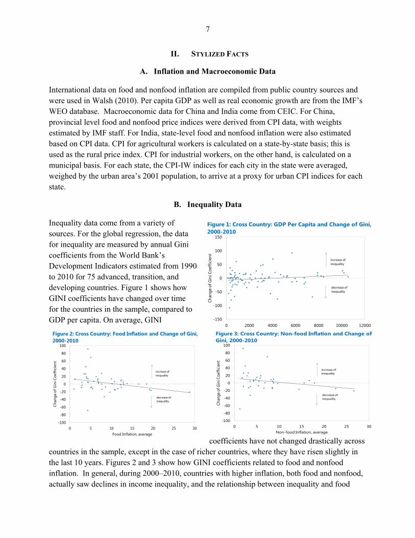
Inequality data come from a variety of sources. For the global regression, the data for inequality are measured by annual Gini coefficients from the World Bank’s Development Indicators estimated from 1990 to 2010 for 75 advanced, transition, and developing countries. Figure 1 shows how GINI coefficients have changed over time for the countries in the sample, compared to GDP per capita. On average, GINI

coefficients have not changed drastically across countries in the sample, except in the case of richer countries, where they have risen slightly in the last 10 years. Figures 2 and 3 show how GINI coefficients related to food and nonfood inflation. In general, during 2000–2010, countries with higher inflation, both food and nonfood, actually saw declines in income inequality, and the relationship between inequality and food

-150

-100

-50

0

50

100

150

0 2000 4000 6000 8000 10000 12000

Chan

ge o

f Gin

i Coe

ffici

ent

GDP Per Capita

Figure 1: Cross Country: GDP Per Capita and Change of Gini, 2000-2010

increase of inequality

decrease of inequality

-100

-80

-60

-40

-20

0

20

40

60

80

100

0 5 10 15 20 25 30

Chan

ge o

f Gin

i Coe

ffic

ient

Food Inflation, average

Figure 2: Cross Country: Food Inflation and Change of Gini, 2000-2010



-100

-80

-60

-40

-20

0

20

40

60

80

100

0 5 10 15 20 25 30

Chan

ge o

f Gin

i Coe

ffici

ent

Non-food Inflation, average

Figure 3: Cross Country: Non-food Inflation and Change of Gini, 2000-2010



8

inflation does not appear significantly different from nonfood inflation, though in these charts other control factors, such as GDP growth, are not yet taken into account.

C. China

Turning to China, rapid economic growth over the past few decades has coincided with a noticeable deterioration in income distribution. The Gini coefficient is estimated to have reached

0.42–0.47 in recent years from below 0.3 in early 1980s3. Cheng (2007) indicated that since 1992 the urban income disparity has replaced the rural income disparity to become the most important driver of overall income inequality. According to his estimates, the urban Gini coefficient increased to 0.33 in 2004 from 0.17 in 1981, while the rural Gini coefficient rose to 0.36 from 0.25 in this period. Meanwhile, the income or expenditure of the richest 10 percent of

the population reached more than13 times of those of the poorest 10 percent in 20054.

Since there is no official publication of Gini coefficients at provincial level, this paper uses provincial Theil indices estimated by the University of Texas to measure inequality. The data cover 31 provinces, municipalities, and autonomous regions over the period 1994–2006. Figure 4 shows that, while GDP per capita grew very rapidly across all Chinese provinces in the first half of the 2000s, most also saw an increase in inequality, with the fastest-growing provinces seeing slightly larger increases in inequality. Figure 5 and 6 show that the change in the Theil index is only slightly correlated with food and nonfood inflation. However, these simple correlations don’t take the (very rapid) growth in income, or other significant macroeconomic and structural factors, into account.

3Estimates of Gini coefficient by international institutions range from 0.42 to 0.47 in 2005–2007. Cheng (2007) estimate the Gini coefficient to be 0.29 in 1981. 4 World Development Indicators.

-1.5

-1.0

-0.5

0.0

0.5

1.0

1.5

2.0

2.5

0 5 10 15 20 25 30 35 40 45Chan

ge o

f Ine

qual

ity (d

eriv

ed fr

om T

heil

Inde

x)

GDP Per Capita

Figure 4. China: Provincial GDP Per Capita and Change of Inequality, 2000-2005

-1.5

-1.0

-0.5

0.0

0.5

1.0

1.5

2.0

2.5

0.5 0.7 0.9 1.1 1.3 1.5 1.7Chan

ge o

f Ine

qual

ity (d

eriv

ed fr

om T

heil

Inde

x)

Inflation

Figure 5. China: Food Inflation and Change of Theil Index, 2000-2005



9

D. India

Indian inequality data come from various government sources and are based on the Indian government’s National Sample Survey Rounds, and cover the period 1990–2004, when India began to open to reforms, though there are not yet income inequality data for the high-growth period of the mid-2000s. Figure 7 shows the pattern of urban and rural inequality across the largest Indian states. Rural inequality is higher than urban inequality in every state, and while rural inequality tends not to vary much across states, urban inequality tends to be greater in the richer states than the poorer ones. Figure 8 shows how per capita income growth between 1994 and 2004 related to changes in income inequality. In general, as with China, inequality rose more in the faster-growing states, and with the breakdown between rural and urban data available, it can be seen that this effect was stronger in urban areas.

E. Other Data

For the international sample, education level is presented as the levels of primary and secondary school enrollment rates from the World Bank’s World Development Indicators database. For China, the picture is more complicated. According to the data published by the China Ministry of Education, primary enrollment ratio changed by a small margin from 108¾ percent in 1994 to 106¼ percent in 2006, meaning that there is little variation over time that can be used in estimation. However, although provincial level data are not published in a comprehensive way, it is believed that western provinces tend to have lower enrollment than more developed provinces in the middle and coastal provinces. And for tertiary education there is some difference: during the period under study, enrollment in higher education

-1.5

-1.0

-0.5

0.0

0.5

1.0

1.5

2.0

2.5

-0.8 -0.6 -0.4 -0.2 0.0 0.2 0.4 0.6 0.8Chan

ge o

f Ine

qual

ity (d

eriv

ed fr

om T

heil

Inde

x)

Inflation

Figure 6. China: Non-food Inflation and Change of Theil Index, 2000-2005


decrease of inequality 0

51015202530354045

0

10

20

30

40

50

60

70

Har

yana

Mah

aras

htra

Guj

arat

Punj

ab

Kera

la

Tam

il N

adu

Karn

atak

a

And

hra

Prad

esh

Utt

ar P

rade

sh

Jam

mu

& K

ashm

ir

Wes

t Ben

gal

Raja

stha

n

Oris

sa

Ass

am

Mad

hya

Prad

esh

Biha

r

GDP per capita (RHS) Rural GINI Urban GINI

Figure 7. India: Inequality and GDP per capita by State

0

5

10

15

20

25

30

-10 -5 0 5 10 15 20

Inco

me

perc

apita

gro

wth

199

4 -

2004

(%)

GINI Change 2004 - 1994

Rural Urban

Figure 8. Per capita GDP growth and change in GINI(16 Indian states, between 1994 and 2004)

10

rose significantly. However, the dramatic mobility of educated workers makes it difficult to gauge the relationship of well educated workers with inequality. Therefore, in this model education level is treated as a province-specific and time-invariant factor. Finally, in India, educational attainment differs more across states than it does in China, and both urban and rural literacy rates are available by state. These data are used in the analysis.

III. METHODOLOGY

The change in inequality over time is measured as the three-year change in GINI coefficients for each country in the sample, with a rising GINI coefficient meaning an increase in income inequality. The three year period is chosen to reduce the volatility from macroeconomic data. The change in GINI is regressed first against headline CPI as a baseline to assess the relationship between inflation and inequality, and then against disaggregated food and nonfood CPI.

The baseline equation estimated is:

y , α λy , X ,′ β ε , (1)

where y denotes the change of Gini coefficients, X includes inflation, food and nonfood, growth in GDP, average level of GDP per capita, and, to control for educational variation, the ratios of primary and secondary school enrollment; ε is the error term. Results are presented under ordinary least squares, as well as for both fixed effects across countries and random effects. However, measuring the relationship between the change of income inequality and income growth itself raises some endogeneity concerns. In particular, Berg and Ostry (2011) suggest that less equal societies are likely to have shorter spells of income growth, implying that the distribution of income may partly determine a particular year’s growth rate. To control for this, the model is also estimated using a Generalized Method of Moments (GMM) dynamic estimator based on the Arellano-Bond (AB) methodology. The methodology specifies a dynamic model which allows for time-invariant country-specific effects, which is plausible in the case of inequality analysis, given that many variables outside the analysis, such as political and tax regime, exhibit minimal variation over time. Under AB the equation is estimated using as instruments the lagged values of the left and right-hand side variables in levels. These instruments are valid if the error term ν is not serially correlated. The specification is:

y , α λy , X ,′ β μ ν , (2)

where μ represents the country specific and time invariant factor and ν is the error term. There

are some statistical shortcomings to a straightforward instrumental variables estimation of the above equation, namely that in a small sample with some persistent explanatory variables, lagged levels make weak instruments for the regression when run in differences. Asymptotically, the variance of the coefficients would rise and coefficients could be biased. To address this

11

weakness, Blundell and Bond (1998) developed the system GMM dynamic model, which combines the regression in first differences above with an estimation run in levels, using both lagged levels and lagged differences as instruments. It was shown that using the system GMM would substantially gain efficiency under certain conditions.

The model used for China is similar, except that instead of country-specific observations and fixed effects across countries, effects are fixed across individual provinces. The dependent variable is the three year moving average change in the Theil index for each province, again chosen to minimize the noise from short term macroeconomic volatility. Income per capita data vary by province and CPI data also vary by province.

For India, the dependent variable is the four-year change in the GINI coefficient for either urban or rural areas for each state, as data are not available at higher frequency. While educational data are available (literacy rates are used) for Indian states, these are dropped in the fixed effects model, where the variation over time is minimal. Growth in real GDP and the average level of per capita GDP for each time interval – which in India are available at the state level - are also included5.

As with the global regression, for both India and China, OLS results are presented alongside fixed- and random-effects GLS estimations, as well as the AB GMM results.

IV. RESULTS

A. International Sample

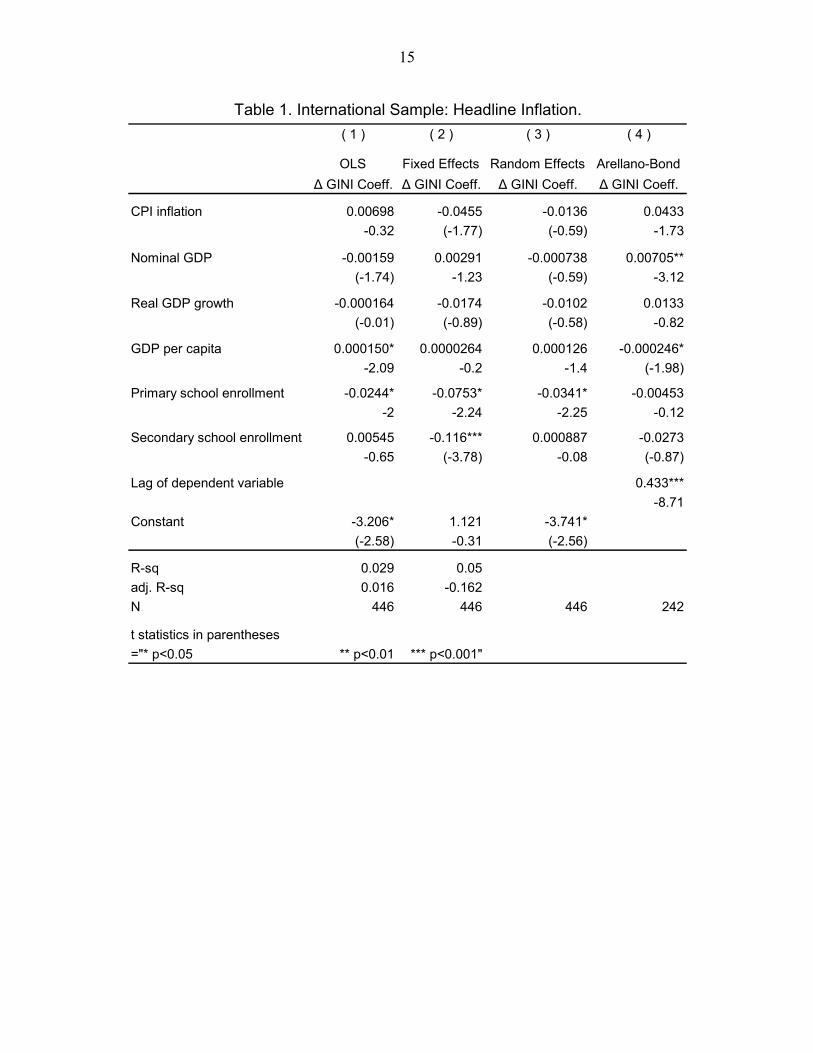
In this sample and analysis, headline inflation does not appear to have a strong relationship with income inequality under most specifications (Table 1). Once simultaneity is taken into account under the Arellano-Bond specification (column 4), higher GDP growth is associated with higher income inequality, while higher GDP per capita is associated with slightly lower income inequality. Higher rates of enrollment in primary education are associated with decreases in income inequality. Secondary school enrollment has a less consistent effect, but when significant is also associated with falling inequality.

Breaking inflation down into food and nonfood inflation produces somewhat different results (Table 2). The relationship between changes in income inequality and food and nonfood inflation is significant only when simultaneity is taken into account under specification (4), and is not consistent across specifications. Nonfood inflation is associated with rising income inequality, the expected result, only under the AB specification. Food inflation is only significant under this specification, and is associated with falling income inequality. Coefficient of GDP per capita is not significant under any specification, while average real GDP growth is associated with slightly lower income inequality in the fixed- and random-effects specifications but not when 5 Other specifications related to income – for example, average growth over time combined with initial level - were also assessed; results were similar.

12

simultaneity is taken into account. Finally, the counterintuitive results about education are no longer present, with secondary school enrollment now intuitively associated with somewhat lower income inequality under the Arellano-Bond specification6.

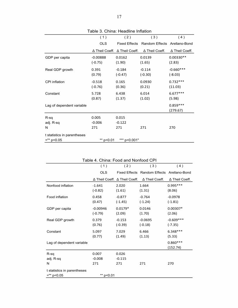
B. China

Turning next to the results from Chinese provinces, once endogeneity is taken into account via the Arellano-Bond specification, higher headline inflation is associated with more rapid widening of inequality, as measured by a Theil coefficient (Table 3). Higher GDP growth is associated with a slower pace of deterioration in income inequality, while richer provinces tend to have bigger increases.

When inflation is divided into food and nonfood inflation, the picture is somewhat different (Table 4). The coefficient on nonfood inflation has the expected positive sign in three of the four specifications, but is only significant under the AB GMM specification. Food inflation is associated with less income inequality under each specification, but this is not significant. As in the headline CPI regressions, faster GDP growth is associated with declining inequality while this effect is mitigated in richer provinces, where inequality tends to rise faster.

C. India

Indian income inequality data are available not only on a state level but also broken down between urban and rural areas, allowing for some distinction between food-producing and food-importing regions.

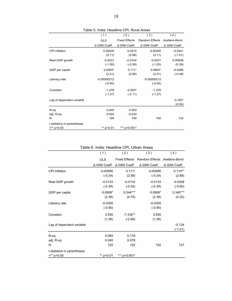
Tables 5 and 6 show the relationship between headline CPI and income inequality (as measured with GINI coefficients) across rural and urban areas in Indian states. In rural areas (Table 5) headline inflation shows little relation with income inequality, with the coefficient very close to zero except under the Arellano Bond specification. Higher income per capita is associated with higher inequality under three specifications, however. Moving to urban areas (Table 6), the results are more intuitive: the coefficient on headline inflation is positive and significant under two specifications, including when accounting for simultaneity, while higher levels of per capita income are also associated with rising income inequality. Literacy and real GDP growth are not generally significant.

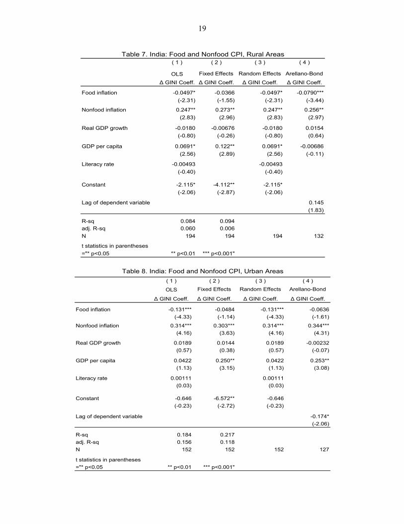
When CPI is divided into food and nonfood inflation, the results are stronger. In rural areas (Table 7), food inflation is strongly linked to lower income inequality, while nonfood inflation, intuitively, is linked to higher income inequality. Again, states with higher levels of per capita income are associated with rising income inequality, though real GDP growth itself, as well as literacy, are not.

6 This in itself may be surprising as access to primary education might be expected to be a more important driver of reducing income inequality than secondary or tertiary education.

13

In urban areas, again as expected higher nonfood inflation is strongly tied to higher levels of income inequality (Table 8). Food inflation, on the other hand, is more ambiguous. The coefficient on food inflation is negative in all specifications, implying that wages are flexible and respond to higher food prices, though the result is significant only in two specifications, and not under Arellano-Bond. As with rural inflation, states with higher levels of income appear to have rising income inequality, while GDP growth and literacy have little effect.

V. CONCLUSION

The results here are relatively agnostic about whether headline inflation is detrimental to income inequality, but are able to extend the analysis beyond this broad measure of inflation. Higher nonfood inflation is associated with worsening income inequality in all three samples (international, India and China), supporting the results from previous work suggesting that income inequality is aggravated by higher levels of inflation. This is intuitive, given that an individual household’s income can benefit from higher prices only for the goods or services that it produces, and no individual is likely to be a producer of a sufficiently wide share of the country’s nonfood consumption basket.

However, this detrimental impact is less for food inflation. In the international sample, and once the endogeneity of inflation, inequality and growth are taken into account, higher food inflation is associated with declining income inequality, and the same is true for Chinese data. These results suggest that food inflation may not be bad for all lower-income people, or at least that the hit to income taken by some groups may be balanced or even exceeded by increased income accruing to other groups, such as low-income food producers.

The Indian data allow some finer conclusions to be drawn. By differentiating between urban and rural inequality, they provide further support that nonfood inflation widens income inequality in both urban and rural areas. Food inflation has different effects, however. The effect on urban inequality is ambiguous, but in rural areas it is strongly associated with lower inequality. This is somewhat counterintuitive: since few urban dwellers are likely to be food producers, it seems reasonable to expect higher food prices to have a negative effect on households that are most exposed to food prices, i.e., the poor, but here the effect of rising food prices on urban inequality does not appear to be particularly strong. And in rural areas, the effect appears to be strongly positive (in the sense of lower inequality).

These results should also be taken with a number of caveats. India and China are relatively closed economies in terms of staple foods. Countries that import a large share of their staple crops, such as wheat or corn, may have very different dynamics of food prices and income inequality than countries where some important staple crops (rice in both countries, and in India, also pulses) are not as susceptible to global commodity shocks. Unlike corn or wheat, the global market for rice and pulses is small and relatively unimportant; beyond that even differing provinces or states in India and China have limited substitutability of crops. Thus self sufficiency

14

means that India and China are likely have higher a share of households producing staple crops as countries that either export or are reasonably self-sufficient in staples. Even within India and China, the effect of food inflation is also likely to be greatest in food importing states and provinces, though this would have to be studied using household data across states or provinces.

Finally, India and particularly China, as relatively high growth economies, may have a different relationship between food production and rural wages. With relatively good opportunities for labor in urban areas and, especially in China, rising agricultural productivity, the ease with which unskilled workers are able to shift from the rural to the urban labor force may be greater than in other countries, muting increases in income inequality in rural areas and providing more of a safety valve for rural workers than would exist in countries with slower growth. With more limited employment opportunities in urban areas, food inflation could be significantly more immiserating for rural consumers in slower-growing economies.

15

( 1 ) ( 2 ) ( 3 ) ( 4 )

OLS Fixed Effects Random Effects Arellano-Bond

∆ GINI Coeff. ∆ GINI Coeff. ∆ GINI Coeff. ∆ GINI Coeff.

CPI inflation 0.00698 -0.0455 -0.0136 0.0433

-0.32 (-1.77) (-0.59) -1.73

Nominal GDP -0.00159 0.00291 -0.000738 0.00705**

(-1.74) -1.23 (-0.59) -3.12

Real GDP growth -0.000164 -0.0174 -0.0102 0.0133

(-0.01) (-0.89) (-0.58) -0.82

GDP per capita 0.000150* 0.0000264 0.000126 -0.000246*

-2.09 -0.2 -1.4 (-1.98)

Primary school enrollment -0.0244* -0.0753* -0.0341* -0.00453

-2 -2.24 -2.25 -0.12

Secondary school enrollment 0.00545 -0.116*** 0.000887 -0.0273

-0.65 (-3.78) -0.08 (-0.87)

Lag of dependent variable 0.433***

-8.71

Constant -3.206* 1.121 -3.741*

(-2.58) -0.31 (-2.56)

R-sq 0.029 0.05

adj. R-sq 0.016 -0.162

N 446 446 446 242

t statistics in parentheses

="* p<0.05 ** p<0.01 *** p<0.001"

Table 1. International Sample: Headline Inflation.

16

( 1 ) ( 2 ) ( 3 ) ( 4 )



Food inflation -0.0338 0.208 0.0377 -0.233*

(-0.27) -1.26 -0.3 (-2.59)

Nonfood inflation -0.0549 -0.325* -0.171 0.318**

(-0.45) (-2.08) (-1.34) -2.86

Nominal GDP -0.00387 0.00625 -0.00232 0.00346

(-1.30) -0.62 (-0.57) -0.71

Real GDO growth -0.0924 -0.153* -0.145* 0.0372

(-1.58) (-2.17) (-2.42) -1.06

GDP per capita 0.0000428 -0.0000498 0.0000931 0.0000068

-0.33 (-0.21) -0.63 -0.06

Primary school enrollment -0.0944* -0.116 -0.0991 -0.101

(-1.99) (-0.67) (-1.57) (-1.22)

Secondary school enrollment 0.00534 -0.129 0.000702 -0.139*

-0.17 (-1.20) -0.02 (-2.17)


-3.67

Constant 11.52* 25.65 12.55*

-2.36 -1.32 -1.97

R-sq 0.086 0.132

adj. R-sq 0.016 -0.15

N 99 99 99 59


="* p<0.05 ** p<0.01 *** p<0.001"

Table 2. International Sample: Food and Nonfood CPI

17

( 1 ) ( 2 ) ( 3 ) ( 4 )


∆ Theil Coeff. ∆ Theil Coeff. ∆ Theil Coeff. ∆ Theil Coeff.

GDP per capita -0.00888 0.0162 0.0139 0.00330**

(-0.75) (1.90) (1.65) (2.83)

Real GDP growth 0.391 -0.184 -0.114 -0.660***

(0.79) (-0.47) (-0.30) (-8.03)

CPI inflation -0.518 0.165 0.0930 0.732***

(-0.76) (0.36) (0.21) (11.03)

Constant 5.728 6.438 6.014 6.677***

(0.87) (1.37) (1.02) (5.98)


(279.67)

R-sq 0.005 0.015

adj. R-sq -0.006 -0.122

N 271 271 271 270


="* p<0.05 ** p<0.01 *** p<0.001"

Table 3. China: Headline Inflation

( 1 ) ( 2 ) ( 3 ) ( 4 )


∆ Theil Coeff. ∆ Theil Coeff. ∆ Theil Coeff. ∆ Theil Coeff.

Nonfood inflation -1.641 2.020 1.664 0.995***

(-0.82) (1.61) (1.31) (8.06)

Food inflation 0.458 -0.877 -0.764 -0.0978

(0.47) (-1.45) (-1.24) (-1.81)

GDP per capita -0.00946 0.0179* 0.0146 0.00307*

(-0.79) (2.09) (1.70) (2.06)

Real GDP growth 0.379 -0.153 -0.0695 -0.609***

(0.76) (-0.39) (-0.18) (-7.35)

Constant 5.097 7.029 6.466 6.348***

(0.77) (1.49) (1.13) (5.33)


(152.74)

R-sq 0.007 0.026

adj. R-sq -0.008 -0.115

N 271 271 271 270


="* p<0.05 ** p<0.01

Table 4. China: Food and Nonfood CPI

18

( 1 ) ( 2 ) ( 3 ) ( 4 )



CPI inflation 0.00200 0.0215 0.00200 -0.0341

(0.11) (0.98) (0.11) (-1.41)

Real GDP growth -0.0231 -0.0104 -0.0231 0.00936

(-1.00) (-0.39) (-1.00) (0.39)

GDP per capita 0.0604* 0.111* 0.0604* -0.0288

(2.21) (2.60) (2.21) (-0.48)

Literacy rate -0.00000212 -0.00000212

(-0.00) (-0.00)

Constant -1.276 -2.953* -1.276

(-1.27) (-2.11) (-1.27)

Lag of dependent variable 0.162*

(2.04)

R-sq 0.045 0.053

adj. R-sq 0.024 -0.033

N 194 194 194 132


="* p<0.05 ** p<0.01 *** p<0.001"

Table 5. India: Headline CPI, Rural Areas

( 1 ) ( 2 ) ( 3 ) ( 4 )



CPI inflation -0.00995 0.111* -0.00995 0.114**

(-0.34) (2.58) (-0.34) (2.69)

Real GDP growth -0.0133 -0.0132 -0.0133 -0.0308

(-0.39) (-0.35) (-0.39) (-0.85)

GDP per capita 0.0908* 0.344*** 0.0908* 0.345***

(2.38) (4.75) (2.38) (4.22)

Literacy rate -0.0305 -0.0305

(-0.90) (-0.90)

Constant 3.550 -7.336** 3.550

(1.28) (-2.99) (1.28)

Lag of dependent variable -0.124

(-1.41)

R-sq 0.065 0.176

adj. R-sq 0.040 0.078

N 152 152 152 127


="* p<0.05 ** p<0.01 *** p<0.001"

Table 6. India: Headline CPI, Urban Areas

19

( 1 ) ( 2 ) ( 3 ) ( 4 )



Food inflation -0.0497* -0.0366 -0.0497* -0.0790***

(-2.31) (-1.55) (-2.31) (-3.44)

Nonfood inflation 0.247** 0.273** 0.247** 0.256**

(2.83) (2.96) (2.83) (2.97)

Real GDP growth -0.0180 -0.00676 -0.0180 0.0154

(-0.80) (-0.26) (-0.80) (0.64)

GDP per capita 0.0691* 0.122** 0.0691* -0.00686

(2.56) (2.89) (2.56) (-0.11)

Literacy rate -0.00493 -0.00493

(-0.40) (-0.40)

Constant -2.115* -4.112** -2.115*

(-2.06) (-2.87) (-2.06)

Lag of dependent variable 0.145

(1.83)

R-sq 0.084 0.094adj. R-sq 0.060 0.006

N 194 194 194 132


="* p<0.05 ** p<0.01 *** p<0.001"

Table 7. India: Food and Nonfood CPI, Rural Areas

( 1 ) ( 2 ) ( 3 ) ( 4 )



Food inflation -0.131*** -0.0484 -0.131*** -0.0636

(-4.33) (-1.14) (-4.33) (-1.61)

Nonfood inflation 0.314*** 0.303*** 0.314*** 0.344***

(4.16) (3.63) (4.16) (4.31)

Real GDP growth 0.0189 0.0144 0.0189 -0.00232

(0.57) (0.38) (0.57) (-0.07)

GDP per capita 0.0422 0.250** 0.0422 0.253**

(1.13) (3.15) (1.13) (3.08)

Literacy rate 0.00111 0.00111

(0.03) (0.03)

Constant -0.646 -6.572** -0.646

(-0.23) (-2.72) (-0.23)

Lag of dependent variable -0.174*

(-2.06)

R-sq 0.184 0.217

adj. R-sq 0.156 0.118

N 152 152 152 127


="* p<0.05 ** p<0.01 *** p<0.001"

Table 8. India: Food and Nonfood CPI, Urban Areas

20

REFERENCES

Albanesi, S. (2001). “Inflation and Inequality.” Luxembourg Income Study Working Paper No. 323.

Berg, A. and J.D. Ostry (2011). “Inequality and Unsustainable Growth: Two Sides of the Same Coin?” International Monetary Fund Staff Discussion Note 11/08.

Blejer, M. and I. Guerrero (1990). “The impact of macroeconomic policies on income distribution: An empirical study of the Philippines.” Review of Economics and Statistics, vol. 72(3), 414-423.

Braumann, B. (2000). “Real Effects of High Inflation.” IMF Working Paper 2000/85.

Cardoso, E., R. Paes de Barros and A. Urani. (1995) “Inflation and Unemployment as Determinants of Inequality in Brazil: The 1980s.” Reform, Recovery and Growth: Latin America and the Middle East, 151-176. University of Chicago Press.

Cheng, Yonghong (2007) “Evolution of Gini Coefficient Since the Start of the Reform and Its Urban-Rural Decomposition”, Social Sciences in China 2007/04.

Christiaensen, L., and L. Demery (2006) “Down to Earth: Agriculture and Poverty Reduction in Africa,” Directions in Development. Washington DC: World Bank.

Datt, G. and M. Ravaillion (1998). “Farm Productivity and Rural Poverty in India,” Journal of Development Studies, vol. 34, 62-85.

Dolmas, J. et al. (1997) “Inequality, Inflation, and Central Bank Independence.” Federal Reserve Bank of Dallas, Research Working Paper 97-05.

Deaton, A. (1989). “Rice Prices and Income Distribution in Thailand: A Non-Parametric Analysis.” The Economic Journal, vol. 99(395), 1-37.

Easterly, W. and S. Fischer (2000). “Inflation and the Poor,” NBER Working Paper 2335.

Ferreira, F.H.G., P.G. Leite, and J.A. Litchfield (2007). “The Rise and Fall of Brazilian Inequality: 1981-2004.” Macroeconomic Dynamics, June 2007, 1-32.

Ferreira, F.H.G., and J.A. Litchfield (2000). “Desigualdade, pobreza e bem-estar social no Brasil: 1981/95.” Desigualdade e Pobreza no Brasil. Rio de Janeiro: IPEA.

Ivanic, M. and W. Martin (2008). “Implications of Higher Global Food Prices for Poverty in Low-Income Countries.” World Bank Policy Research Working Paper 4594.

Neri, M. 1995 (1995) “Sobre a mesuração dos salários reais em alta inflação.” Pesquisa e Planejamento Econômico 25(3), 497-525.

21

Rashid, S. (2002) “Dynamics of Agricultural Wage and Rice Prices in Bangladesh: A Reexamination.” International Food Policy Research Institute Discussion Paper No. 44.

Ravallion, M. (2000) “Prices, wages and poverty in rural India: what lessons do the time series data hold for policy?” Food Policy, vol. 25, 351-364.

Romer, C.D. and D.H. Romer (1998) “Monetary Policy and the Well-Being of the Poor.” NBER Working Paper 6793.

Walsh, J.P. (2010). “Reconsidering the Role of Food Prices in Inflation.” IMF Working Paper 11/71.

Warr, P. (2005) “Food Policy and Poverty in Indonesia: A General Equilibrium Analysis.” Australian Journal of Agricultural and Reserouce Economics, vol. 49(4): 429-51.

Woden Q.C., et al., (2008) “Potential Impact of Higher Food Prices on Poverty: Summary Estimates for a Dozen West African Countries,” mimeo, World Bank, Washington DC.

Wodon, Q., and H. Zaman (2008). “Rising Food Prices in Sub-Saharan Africa: Poverty Impact and Policy Responses.” World Bank Policy Research Paper 4738.

inflation and income inequality: is food inflation … and income inequality: is food inflation...

Documents