inflation anchoring, real borrowing costs, and growth

1

Inflation Anchoring, Real Borrowing Costs, and

Growth: Evidence from Sectoral Data*

Sangyup Choi Davide Furceri• Prakash Loungani$

Yonsei University IMF IMF

June 2019

Abstract

Central bankers often assert that anchoring of inflation expectations and reducing inflation

uncertainty are good for economic outcomes. We test this claim and search for a relevant

channel using panel data on sectoral growth for 22 manufacturing industries from 36

advanced and emerging market economies over the period 1990-2014. Our difference-in-

difference strategy is based on the theoretical prediction that inflation uncertainty has larger

effects in industries that are more credit constrained by increasing effective real borrowing

costs. The results show that industries characterized by high external financial dependence,

low asset tangibility, and high R&D intensity tend to grow faster in countries with well-

anchored inflation expectations. The results are robust to controlling for the interaction

between these characteristics and a broad set of macroeconomic variables over the sample

period, including the level of inflation and output volatility. The results are also robust to IV

techniques, using indicators of monetary policy transparency and independence as

instruments.

Keywords: industry-level growth; inflation anchoring; inflation uncertainty; long-run

growth; credit constraints.

JEL codes: E52; E63; O11; O43; O47.

* We are thankful to Grace Bin Li, Chansik Yoon, Bok-Keun Yu, Carlos Vegh, Guillermo Vuletin, and the

seminar participants at the Bank of Korea. This paper was supported in part through a research project on

macroeconomic policy in low-income countries with the U.K.’s Department for International Development. The

views expressed in this paper are those of the authors and should not be reported as representing the views of

the IMF or DFID. The usual disclaimer applies and any remaining errors are the authors’ sole responsibility.

School of Economics, Yonsei University, 50 Yonsei-ro, Seodaemun-gu, Seoul 03722, South Korea. Email

address: [email protected]. • International Monetary Fund, 700 19th street NW, 20431 Washington D.C. Email address: [email protected]. $ International Monetary Fund, 700 19th street NW, 20431 Washington D.C. Email address: [email protected].

mailto:[email protected]



2

“The extent to which inflation expectations are anchored has first-order implications for the

performance … of the economy” (Bernanke, July 10, 2007)

“To the extent that a monetary authority can build a reputation and gain credibility for low

inflation, it … produces tangible economic benefits” (Plosser, April 10, 2007)

I. INTRODUCTION

Central bankers often assert that low and stable inflation fosters macroeconomic

stability and growth. Former Fed Chairman Paul Volcker stated that: “Inflation feeds in part

on itself, so part of the job of returning to a more stable and more productive economy must

be to break the grip of inflationary expectations.” (Volcker, statement before the Joint

Economic Committee of the U.S. Congress, October 17, 1979). The important role of

inflation expectations has led many central banks around the world to improve transparency

regarding the central bank’s goals, often explicitly through the adoption of an inflation target

(IT) and better communication with economic agents.1

This view is underpinned by a large body of the theoretical literature suggesting that

inflation uncertainty makes it difficult for firms to plan in advance (Fisher and Modigliani,

1978; Baldwin and Ruback, 1986; Huizinga, 1993). Thus, firms may reduce or delay

investment when uncertainty about future prices is high. While it is well established that

heightened uncertainty can distort investment toward more flexible and less growth-

enhancing factors of productions when firms are credit constrained, thereby slowing down

the long-run growth of the economy (Aghion et al., 2010, 2014),2 this distortion can be

particularly acute for the case of inflation uncertainty since inflation uncertainty affects

effective real borrowing costs directly.3

1 For the stabilizing effect of inflation targeting, see Bernanke et al. (1999), Mishkin (2000), and Gonçalves and

Salles (2008).

2 See Bernanke (1983) and Pindyck (1988, 1991) for the earlier theoretical contribution to show that that

uncertainty increases the real option value of dealying irreverisble ivnestment.

3 Similar to the theoretical prediction by Aghion et al. (2010), Baldwin and Ruback (1986) show that higher

uncertainty about future relative prices increases short-term investment relative to long-term investment.

3

Higher inflation uncertainty implies a higher likelihood of unexpected inflation in the

future, which would arbitrarily redistribute the wealth between savers and borrowers via the

Fisher equation since the borrowing cost is typically denominated in the nominal value.

Unless financial market participants are risk neutral, higher inflation uncertainty prevents

well-functioning financial markets, which is a distinct consequence of inflation uncertainty

from the consequence of high inflation per se. Thus, the adverse effect of higher inflation

uncertainty could be particularly detrimental for firms that heavily rely on external finance or

do not have sufficient collateral to post.4 We test this theoretical prediction empirically using

a country-level proxy for inflation uncertainty and industry-level measures of credit

constraints and economic outcomes.

Several authors have tried to demonstrate the benefits of low inflation or inflation

uncertainty for growth empirically. For example, Fischer (1993) and Barro (1996) use cross-

section and panel data for a large sample of countries to show that very high inflation was

detrimental to growth, after controlling for other factors, over the period 1960 to 1990.

However, other authors have found it difficult to demonstrate such impacts—particularly in

more recent decades when inflation rates have been lower than in the 1970s and 1980s—or

have found the evidence to be fragile. For example, using an extreme bound analysis, Levine

and Renelt (1992) concluded that inflation variables are not robustly correlated with growth.

Judson and Orphanides (1999) conclude that “the empirical evidence documenting the

benefits of low inflation is not very persuasive.”

The main challenge in identifying causal effects of inflation on growth using

aggregate data is that it is very difficult to control for all possible factors that are correlated

with inflation (or inflation uncertainty) and that at the same time may affect growth. This

paper tries to overcome this limitation by using sectoral (industry-level) data and applying a

difference-in-difference strategy à la Rajan and Zingales (1998). Our conjecture about which

4 Inflation uncertainty can also reduce investment by increasing the firm’s opportunity cost of holding cash. For

example, Berentsen et al. (2012) explore the opportunity cost of holding cash, R&D investment and growth on

the basis of a money search model where liquidity is essential for investing in innovative investment. Chu and

Cozzi (2014) analyze the effect of price uncertainty on economic growth in a Schumpterian model with a cash-

in-advance requirement on R&D investment. However, Dotsey and Sarte (2000) show that in a model where

money is introduced via a cash-in-advance constraint, inflation uncertainty has a positive effect on growth via a

precautionary savings motive, while the level of inflation reduces growth.

4

industries that should benefit more from inflation anchoring (therefore, low inflation

uncertainty) is motivated by recent work by Aghion et al. (2010). Their work suggests that

volatility in the economic environment is particularly harmful to growth for those firms and

industries that are credit constrained, as it pushes them toward short-term investment rather

than long-term investment that boosts long-run growth.

Motivated by this theoretical framework, our empirical analysis examines the sectoral

output growth effect of the interaction between a country’s measure of inflation anchoring

and sector-specific measures of credit constraints, after controlling for the unobserved

country- and sector-specific characteristics. The framework is estimated for an unbalanced

panel of 22 manufacturing industries from 36 advanced and emerging market economies over

the period 1990-2014. As explained above, since inflation uncertainty is particularly relevant

for the channel through which credit constraints determine the optimal allocation between

short- and long-term investment, we expect that credit-constrained industries have achieved

relatively faster growth in a country where inflation expectations are well anchored.

The advantages of a cross-industry analysis compared to a one cross-country are

twofold:

• First, we measure the degree of inflation anchoring by the sensitivity of inflation

expectations to inflation surprises—a unique time-invariant parameter that varies only

across countries. Thus, the country-fixed effect to control for unobserved cross-

country heterogeneity in a standard cross-country analysis absorbs the country-

specific inflation anchoring coefficient, which calls for a more disaggregated level of

analysis.

• Second, it mitigates concerns about reverse causality. While it is difficult to identify

causal effects using aggregate data, it is much more likely that inflation anchoring at

the country level affects its industry-level outcomes than the other way around. Since

we control for country fixed effects—and therefore for aggregate output—reverse

causality in our setup would imply that differences in output across sectors influence

inflation anchoring at the aggregate level—which seems implausible. Moreover, our

main independent variable is the interaction between the degree of inflation anchoring

5

and industry-specific technological characteristics obtained from the U.S. firm-level

data, which makes it even less plausible that causality runs from industry-level

growth to this composite variable.

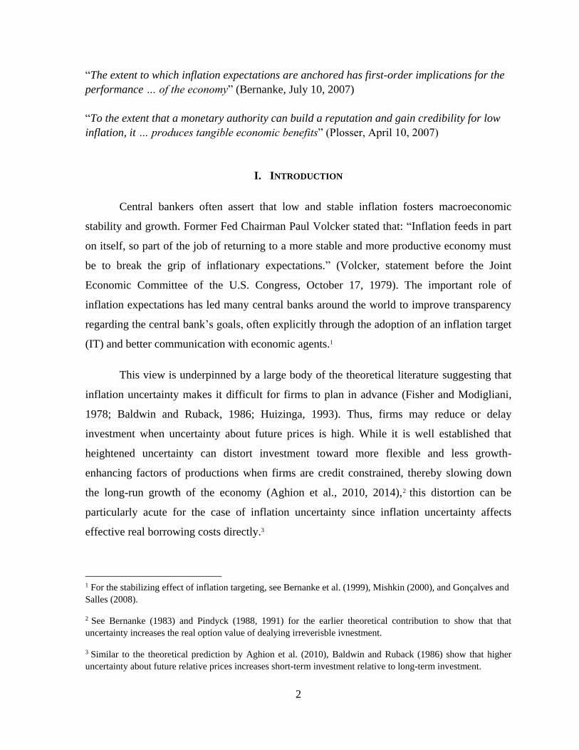
The main finding of our paper is that inflation anchoring fosters growth in industries

that are more credit constrained. Figure 1 summarizes this finding in an intuitive way. In

Figure 1, we plot the average value-added growth of each manufacturing industry from 1990

to 2014 against the sensitivity of inflation expectations in response to inflation surprises—our

measure of inflation anchoring—estimated by each country after controlling for the initial

share of each manufacturing industry.5 While the left panel in Figure 1 plots this relationship

only for industries with the below-median level of external financial dependence (i.e., less

credit constrained industries), the right panel plots the relationship only for industries with

the above-median level of external financial dependence (i.e., more credit constrained

industries). It is clear that higher sensitivity (i.e., higher inflation uncertainty) slows down the

average growth only for industries with the above-median level of external financial

dependence.6

This paper contributes to two streams of literature. The first is on long-lasting

literature on the causal relationship between inflation and growth (Dornbusch and Frenkel,

1973; De Gregorio, 1993; Barro, 1996; Judson and Orphanides,1999; López-Villavicencio

and Mignon, 2011).7 The second is on more recent literature regarding the role of financial

frictions in amplifying the effect of uncertainty about the economic environment—on growth

(Aghion et al., 2014; Christiano et al., 2014; Choi et al., 2018; Choi and Yoon; Arellano et

al., forthcoming).

The rest of the empirical analysis aims at establishing the robustness of this main

finding. First, we extend the measure of credit constraints to include asset tangibility and

5 To be more specific, we regress the average value-added growth of an industry i in a country c on the measure

of inflation anchoring, a set of industry dummies, and the initial share of the industry i in a country c.

6 The slope coefficients of the left (right) panel are 0.82 and -27.69 and the associated t-statistics using robust

standard errors are 0.06 and -2.14, respectively.

7 See Judson and Orphanides (1999) and references therein for a more comprehensive review of the literature.

6

R&D intensity, in addition to external financial dependence shown above. These

characteristics are widely used as a proxy for credit constraints at the industry level (Braun

and Larrain, 2005; Ilyina and Samaniego, 2011; Aghion et al., 2014). Second, we disentangle

the effect of inflation anchoring from the effect of the level of inflation by explicitly

controlling for the interaction between the level of inflation and industry-specific measures of

credit constraints. While these two channels tend to be correlated, since low inflation is often

achieved by better inflation anchoring (or a low-inflation environment fosters well-anchored

inflation expectations), the results of the analysis suggest that is the anchoring of inflation

expectations and not the level of inflation per se that has a statistically significant effect on

growth. The finding that the credit constraint channel operates through inflation anchoring

not the level of inflation supports the theoretical prediction based on the interaction between

inflation uncertainty and real borrowing costs.

The main results are robust to controlling for the interaction between sectoral credit

constraint measures and an additional set of macroeconomic variables that might affect an

industry growth—such as financial development, the size of government, overall economic

growth, monetary policy counter-cyclicality, and output volatility—and to IV techniques,

using monetary policy transparency and independence as instruments. Subsample analyses

further indicate that our findings are not driven by the inclusion of euro-area countries with a

common monetary policy framework during the second half of the sample period or the

recent extreme events, such as the global financial crisis and its aftermath.

The remainder of the paper is organized as follows. Section II outlines the credit

constraint channel through which inflation anchoring can affect growth and its empirical

proxies. Section III describes the underlying data used in the analysis and how we construct

our measure of inflation anchoring. Section IV explains our difference-in-difference

methodology. Section V presents the main results and the results from a battery of robustness

exercises. Section VI provides conclusions.

II. INFLATION ANCHORING AND GROWTH: THE ROLE OF CREDIT CONSTRAINTS

What are the channels through which inflation anchoring affects industry growth? In

principle, inflation anchoring reduces uncertainty regarding the future level of inflation so

7

that firms and households can make more informed decisions regarding their investment and

consumption (or saving), as described in theoretical work by Bernanke (1983), Pindyck

(1988, 1991).

Aghion et al. (2010) further develop this framework by showing that credit frictions

are a key channel through which uncertainty affects long-run growth. In their theory, firms

can invest either in short-term projects or in productivity-enhancing longer-term projects that

are subject to liquidity risk. If credit constraints bind only during periods of contractions,

reducing the volatility of aggregate shocks increases the likelihood that long-term projects

survive liquidity shocks in bad states without affecting what happens in good states (when

credit constraints are not binding). Thus, the higher the fraction of credit constrained firms,

the larger the positive effect of reducing uncertainty (or volatility). This mechanism suggests

that uncertainty about the state of the economy would have larger effects on productivity-

enhancing investment in more credit-constrained industries.

While the above mechanism applies to overall uncertainty regarding the state of the

economy, such as productivity, uncertainty about future inflation can be particularly harmful

to credit-constrained firms since higher inflation uncertainty directly translates into higher

uncertainty in real borrowing costs. The possible realization of higher real borrowing costs is

likely to reduce the investment of more credit-constrained firms than others since it would

prevent well-functioning financial markets through an arbitrary redistribution of the wealth

between savers and borrowers. By focusing on the resolution of a certain kind of (inflation)

uncertainty achieved by inflation anchoring, our empirical analysis strengthens the

identification of the relevant channel of credit constraints, thereby contributing to the existing

literature on the link between uncertainty and growth (Ramey and Ramey, 1995; Imbs, 2007;

Aghion et al., 2010).

Following Aghion et al. (2014) as a benchmark for our analysis, we conduct a similar

industry-level analysis on the channel through which inflation anchoring affects industry

growth. We discuss several intrinsic characteristics at the industry-level that are known to

capture the degree of credit constraints and how they are measured. Our discussion draws

8

largely from previous studies on technology and growth at the industry level (Braun and

Larrain, 2005; Ilyina and Samaniego, 2011; Aghion et al., 2014; Samaniego and Sun, 2015).

External financial dependence

The interaction between firms’ external financial dependence and the macroeconomic

environment has been widely studied in the existing literature (for example, Rajan and

Zingales, 1998; Braun and Larrain, 2005; Ilyina and Samaniego, 2011). Recently, Aghion et

al. (2014) use external financial dependence as a proxy for industry-level credit constraints

and find that industries with a relatively heavier reliance on external finance tend to grow

faster in countries with more countercyclical fiscal policies. To test whether inflation

anchoring has a similar stabilizing effect through the credit constraint channel, it is crucial to

examine the role of external financial dependence. Following Rajan and Zingales (1998),

dependence on external finance in each industry is measured as the median across all U.S.

firms, in each industry, of the ratio of total capital expenditures minus the current cash flow

to total capital expenditures. We use an updated version of this indicator from Tong and Wei

(2011). 8 Based on the previous empirical evidence, we expect a positive sign on the

interaction term between the degree of external finance and the measure of inflation

anchoring.

Asset tangibility

If inflation anchoring affects industry growth through the credit constraint channel,

we should expect that inflation anchoring increases growth more in industries with lower

asset tangibility. This is because intangible assets are harder to use as collateral (Hart and

Moore, 1994) so that an industry with less tangible capital tends to be more credit

constrained. In the presence of high inflation uncertainty, firms without sufficient collateral

are likely to lose their access to external financial markets than firms with sufficient tangible

assets to be collateralized. We take industry-level asset tangibility indicators from Samaniego

and Sun (2015), who updated the values in Braun and Larrain (2005) and Ilyina and

Samaniego (2011) using the ratio of fixed assets to total assets from the U.S. Compustat data.

8 The updated data have been kindly provided by Hui Tong.

9

R&D intensity

R&D-intensive industries can be more credit constrained for several reasons. First,

while R&D typically requires large startup investments, its return often realizes with a

significant lag. In the meantime, firms may find it difficult to finance their operational costs

and are forced to rely on external financing. Second, R&D is an intangible asset that is

difficult to collateralize, which also makes R&D intensive firms difficult to raise external

finance. This channel is also consistent with most of the empirical evidence suggesting a

negative relationship between uncertainty and R&D investment (Goel and Ram, 2001;

Czarnitzki and Toole, 2011; Furceri and Jalles, 2019). We adopt the industry-level indicators

from Samaniego and Sun (2015) who measure R&D intensity as R&D expenditures over

total capital expenditure using the U.S. Compustat data.

III. DATA

A. Measuring the degree of inflation anchoring

We begin by assessing the sensitivity of medium-term inflation expectations in

response to inflation surprises, which serves an inverse measure of inflation anchoring (or a

measure of inflation uncertainty). While most existing studies have relied on the volatility of

inflation as a measure of inflation uncertainty, it is not adequate for studying long-run

economic growth. What is important for a firm’s investment decision is an ex-ante measure

of inflation uncertainty through the Fisher equation, whereas inflation volatility is an ex-post

measure. Such an ex-post measure of inflation uncertainty is subject to a more endogeneity

concern since higher inflation volatility is a likely outcome of poor economic performance.

To better capture the relevance of the credit constraint channel through real borrowing costs

for long-run growth, we measure the so-called “steady state” measure of ex-ante inflation

uncertainty using the degree of inflation anchoring.

Following Levin et al. (2004), we relate changes in inflation expectations to changes

in inflation using forecast data. In particular, the following equation is estimated for each

country i in the sample:

∆𝜋𝑖,𝑡+ℎ𝑒 = 𝛽𝑖

ℎ𝜋𝑖,𝑡𝑛𝑒𝑤𝑠 + 휀𝑖,𝑡+ℎ, (1)

10

where ∆𝜋𝑖,𝑡+ℎ𝑒 denotes the first difference in expectations of inflation h years ahead in the

future, and 𝜋𝑖,𝑡𝑛𝑒𝑤𝑠 is a measure of current inflation shocks—defined as the difference between

actual inflation and short-term inflation expectations from Consensus Economics. We use

survey-based measures of professional forecasters’ inflation expectations from Consensus

Economics that are available at different horizons for a large set of countries.9 The coefficient

𝛽𝑖ℎ captures the degree of anchoring in h-years-ahead inflation expectations—a term usually

referred to as “shock anchoring” (Ball and Mazumder, 2011) with a smaller value of the

coefficient denoting well-anchored inflation expectations or low inflation uncertainty.

The quarterly forecast error is used as a baseline measure of inflation shocks for the

analysis because it is less subject to reverse causality than other measures, such as changes in

inflation or deviations of inflation from target. Nevertheless, we still test the robustness of

our findings by using alternative measures. The sensitivity of inflation expectations for the

survey-based forecast is normalized to measure how much inflation expectations are updated

in response to a one percentage point change in inflation. The baseline specification is

estimated using five-year-ahead inflation expectations from Consensus Economics, for two

reasons: i) inflation expectations at this horizon are a close proxy for central banks’ inflation

targets, so that the parameter β can be interpreted as the degree to which the headline

inflation is linked to the central bank’s target—a phenomenon typically referred to as “level

anchoring” (Ball and Mazumder, 2011) and ii) medium-term inflation expectations are less

correlated with current and lagged inflation and hence are less subject to problems of

multicollinearity and reverse causality.10

If monetary policy is credible, the value of this parameter at a sufficiently long

horizon should be close to zero. That is, inflation shocks should not lead to changes in

medium-term expectations if agents believe that the central bank can counteract any short-

term developments to bring inflation back to the target over the medium term. Given the

uncertainty about the relevant horizon for firms’ pricing decisions and in light of the previous

results, we use inflation expectations at various horizons. The model is estimated for each

9 See IMF (2016) for further details on how Consensus forecasts are constructed.

10 We check the sensitivity of the results to alternative horizons in the robustness check section.

11

advanced and emerging market economy for which survey-based inflation expectation data

are available, which produces estimates for 44 countries where Consensus Forecasts are

available from 1990 to 2014.

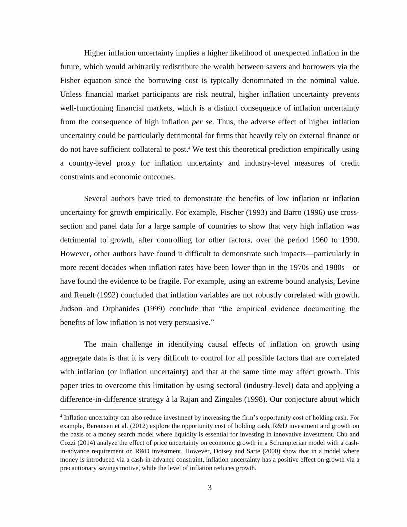
In Figure 2, we first present the evolution of the left-hand-side (top panel) and right-

hand-side (bottom panel) variables in equation (1) for advanced and emerging market

economies. Not surprisingly, changes in inflation expectations have been more volatile at

shorter horizons for both groups of countries. Expectations were on a downward path

throughout the 1990s in both advanced and emerging market economies as monetary

frameworks were improving and actual inflation was falling. This trend was particularly

strong in emerging market economies. Inflation expectations have been remarkably stable

throughout the 2000s in advanced economies, especially at longer horizons, but recently their

volatility has somewhat increased. In contrast, for emerging market economies the volatility

of expectations during 2009–14 has been lower than in the previous decade.

Inflation shocks have been relatively modest in advanced economies, except for the

period surrounding the global financial crisis. These shocks were mostly negative in the

1990s, suggesting that realized inflation was generally lower than expected inflation but have

been close to zero in the 2000s. Since 2011, the median inflation shock in advanced

economies has become negative again. In emerging market economies, inflation shocks were

negative on average in the 1990s and early 2000s, but less so more recently.

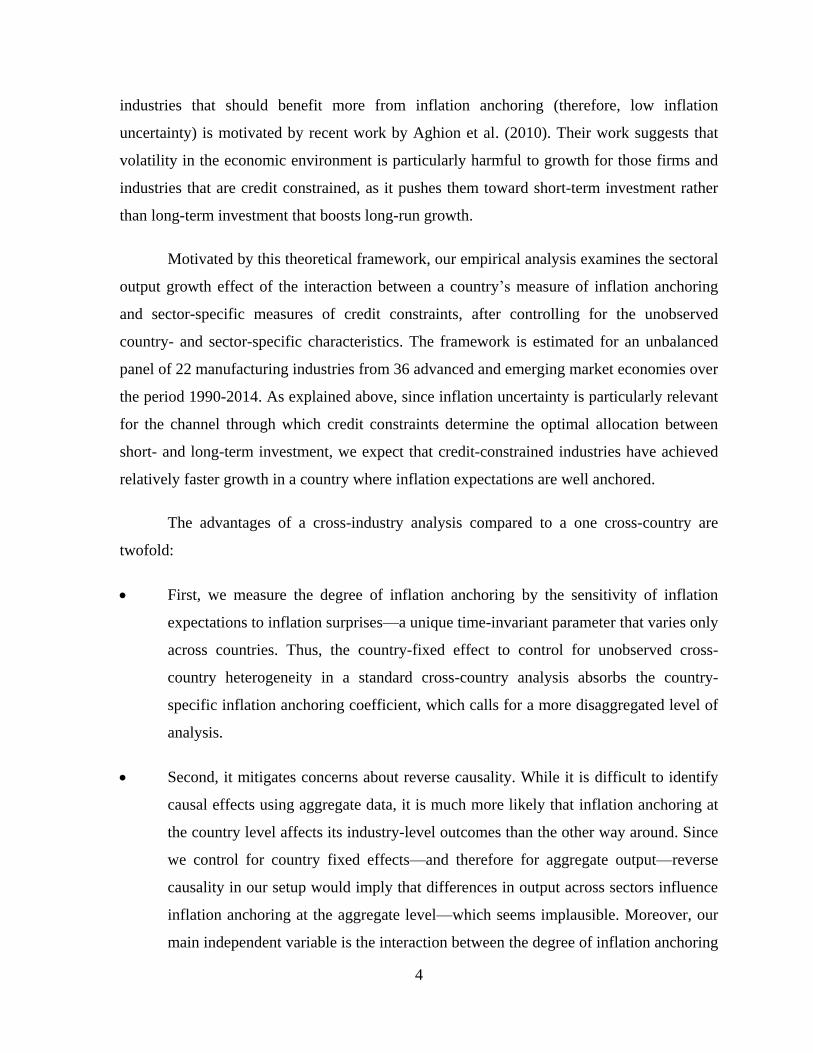
In Figure 3, we show the coefficient of the sensitivity of medium-term inflation

expectations (or a steady-state measure of inflation uncertainty) estimated in equation (1) for

the final sample of 36 countries used in the analysis. While the average of the sensitivity

coefficients is 0.03, their standard deviation is 0.05, implying large variations across

countries. As shown, there is considerable heterogeneity in the size of the sensitivity among

countries, with advanced economies having stronger inflation anchoring than emerging

market economies. We will exploit this cross-country variation to identify the causal effect of

inflation anchoring on sectoral growth.11

11 Table A.1 in the appendix provides the estimates of 𝛽𝑖

ℎ for all available horizons h and country i.

12

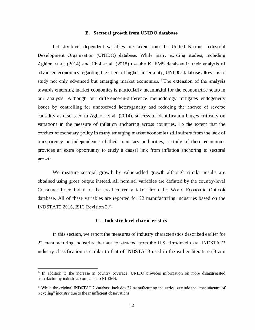
B. Sectoral growth from UNIDO database

Industry-level dependent variables are taken from the United Nations Industrial

Development Organization (UNIDO) database. While many existing studies, including

Aghion et al. (2014) and Choi et al. (2018) use the KLEMS database in their analysis of

advanced economies regarding the effect of higher uncertainty, UNIDO database allows us to

study not only advanced but emerging market economies.12 The extension of the analysis

towards emerging market economies is particularly meaningful for the econometric setup in

our analysis. Although our difference-in-difference methodology mitigates endogeneity

issues by controlling for unobserved heterogeneity and reducing the chance of reverse

causality as discussed in Aghion et al. (2014), successful identification hinges critically on

variations in the measure of inflation anchoring across countries. To the extent that the

conduct of monetary policy in many emerging market economies still suffers from the lack of

transparency or independence of their monetary authorities, a study of these economies

provides an extra opportunity to study a causal link from inflation anchoring to sectoral

growth.

We measure sectoral growth by value-added growth although similar results are

obtained using gross output instead. All nominal variables are deflated by the country-level

Consumer Price Index of the local currency taken from the World Economic Outlook

database. All of these variables are reported for 22 manufacturing industries based on the

INDSTAT2 2016, ISIC Revision 3.13

C. Industry-level characteristics

In this section, we report the measures of industry characteristics described earlier for

22 manufacturing industries that are constructed from the U.S. firm-level data. INDSTAT2

industry classification is similar to that of INDSTAT3 used in the earlier literature (Braun

12 In addition to the increase in country coverage, UNIDO provides information on more disaggregated

manufacturing industries compared to KLEMS.

13 While the original INDSTAT 2 database includes 23 manufacturing industries, exclude the “manufacture of

recycling” industry due to the insufficient observations.

13

and Larrain, 2005; Ilyina and Samaniego, 2011), with a minor exception.14 For example,

whereas “manufacture of food products and beverages” (ISIC 16) is the first industry in the

INDSTAT2 dataset, the INDSTAT3 dataset disaggregates them into “manufacture of food

products” (ISIC 311) and “manufacture of beverages” (ISIC 313). Following Choi et al.

(2017), we take the average of the industry characteristics for ISIC 311 and ISIC 313 to

obtain the value for ISIC 16 in this case. If two datasets share the same industry, we simply

use the values of INDSTAT3. Table A.2 in the appendix compares the industry classification

between INDSTAT2 and INDSTAT3.

We draw on Rajan and Zingales (1998), Braun and Larrain (2005), Ilyina and

Samaniego (2011), and Samaniego and Sun (2015) to compute industry-level indicators.

Table 1 reports the measures of industry characteristics. Table 2 shows the correlation matrix

amongst these variables. The correlations amongst industry characteristics measures are

intuitive and consistent with what existing theories would predict. For example, as described

in Choi et al. (2018), an industry that relies more heavily on external finance also tends to

have lower asset tangibility and higher R&D intensity. However, this correlation is far from

perfect. For example, the correlation between external financial dependence and asset

tangibility is only -0.27.

Our final sample consists of an unbalanced panel of 36 countries in which the

consistent data are available for both Consensus Economics and UNIDO. Table 3

summarizes the final country coverage and the number of observations used in the analysis

per country. We do not include the U.S. in the final sample, as the industrial characteristics

are measured from U.S. firm-level data. To the extent that inflation anchoring in the U.S.

influence U.S. firms from different industries in a systematic way, the inclusion of the U.S.

would bias the result.

IV. METHODOLOGY

To assess the effect of inflation anchoring on sectoral growth and identify the relevant

transmission channels, the analysis follows the methodology proposed by Rajan and Zingales

14 There are 28 manufacturing industries in INDSTAT3.

14

(1998). The following specification is estimated for an unbalanced panel of 36 countries and

22 manufacturing industries:

𝑔𝑖,𝑐 = 𝛼𝑖 + 𝛼𝑐 + 𝛿𝑋𝑖𝑖𝑛𝑓𝑐 + 𝜇𝑦𝑖,𝑐0 + 휀𝑖,𝑐 , (2)

where i denotes industries and c denotes countries. 𝑔𝑖,𝑐 is a measure of industry growth,

which is the average value-added growth from 1990 to 2014; 𝑦𝑖,𝑐0 is the initial share of each

manufacturing sector i of country c’s total manufacturing output in 1990; 𝑋𝑖 is a measure of

an industry characteristic for industry i, such as external financial dependence; 𝑖𝑛𝑓𝑐 is our

measure of inflation anchoring for country c;15 𝛼𝑖 and 𝛼𝑐 are industry and country fixed

effects, respectively.

Following Dell'Ariccia et al. (2009), Equation (2) is estimated using OLS—and

standard errors are clustered at the country level—as the inclusion of fixed effects is likely to

address the endogeneity concerns related to omitted variable bias.16 Also, reverse causality

issues are unlikely. First, related to the measures of industry characteristics, it is hard to

conceive that sectoral growth in other countries can influence a particular U.S. industry’s

intrinsic characteristics. Second, it is very unlikely that growth at the sectoral level can

influence the aggregate measures of inflation anchoring. Claiming reverse causality is

equivalent to arguing that differences in growth across sectors lead to differences in the

degree of inflation anchoring—which we believe to be unlikely.

Since the industry characteristics are measured using only U.S. firm-level data, one

potential problem with this approach is that U.S. industry characteristics may not be

representative of the whole sample. While this issue is unlikely to be important for advanced

economies, extending it to developing economies requires caution. Nevertheless, using

country-specific industry-level characteristics, even if such measures are available, does not

necessarily improve identification. For example, it is plausible that growth in the textile

industry in China affects systematically its own set of characteristics than the characteristics

15 A higher sensitivity coefficient means a lower degree of inflation anchoring.

16 Table A.3 in the appendix shows that clustering standard errors at the industry level hardly changes the main

results.

15

of the U.S. textile industry. Thus, using country-specific characteristics may exacerbate the

endogeneity issue. It is important to note that U.S. measures of industrial characteristics are

assumed to represent technological characteristics in a frictionless environment, thereby

serving as a conceptual benchmark for our analysis.

However, a remaining possible concern in estimating equation (2) with OLS is that

other macroeconomic variables could affect industry growth when interacted with industries’

certain characteristics and they are also correlated with our inflation anchoring measure. For

example, this concern could be the case for financial development—the original channel

assessed by Rajan and Zingales (1998)—but also for the level of inflation itself or the stance

of monetary policy. We address this issue in the subsection devoted to robustness checks.

V. RESULTS

A. Baseline results

Table 4 presents the results obtained by estimating equation (2). They report the

interaction effects of inflation anchoring and various industrial characteristics capturing the

credit constraint channel on sectoral growth, together with the convergence coefficient on the

initial share of the industry. The main findings are summarized as follows. First, convergence

exists strongly, as the coefficient on the initial share is negative and statistically significant at

the one percent level. Second, the signs of the interaction terms are consistent with the credit

constraint channel. We find that inflation anchoring—that is, the lower sensitivity of inflation

expectations in response to inflation surprises—increases growth more for industries with i)

higher external financial dependence, ii) lower asset tangibility, iii) higher R&D intensity.

The effects through these three channels are statistically significant at the five percent level.

Our finding corroborates Dedola and Lippi (2005) who find that sectoral output response to

monetary policy shocks is systematically related to the degree of an industry-level credit

constraint, including external financial dependence.

To gauge the magnitude of each channel, we measure differential growth gains from a

decrease in the sensitivity coefficient from the 75th to the 25th percentile of the distribution

for an industry at the 75th percentile of the distribution compared to the industry at the 25th

percentile in their intrinsic characteristics. The magnitude of the interaction effects of

16

inflation anchoring ranges from 0.6 for asset tangibility to 1.2 percentage points for external

financial dependence. For example, the results suggest that the differential growth gains are

1.2 percentage point by improving inflation anchoring from the level of Czech Republic to

that of Italy and simultaneously moving from an industry with low external financial

dependence to an industry with high external financial dependence. While these magnitudes

seem large at first glance, moving from the 75th to the 25th percentile in the sensitivity of

inflation expectations implies a quite dramatic enhancement in the credibility of monetary

policy, which is unlikely to happen in any individual country over a short period.

B. Robustness checks

Alternative growth measure

While value-added measures an industry’s ability to generate income and contribute

to GDP, gross output principally measures overall production at market prices. The

difference between gross output and value added of an industry is intermediate inputs. To the

extent that the intensity of intermediate inputs varies across countries within the same

industry, our growth measure based on value-added might not necessarily give us the same

picture as a gross output measure. To check this possibility, we repeat our analysis using the

average growth rate of gross output. Gross output is also deflated using the CPI to obtain real

values. Table 5 confirms that the sign, size, and statistical significance of the interaction

effects using gross output are largely similar to those using value added, lending support to

our baseline results. The only difference is that the asset tangibility channel is no longer

statistically significant.

Subsample analysis

We further test the robustness of our findings to two alternative subsample analyses.

First, our finding might have been driven by the extreme event of the global financial crisis

and constrained monetary policy in many advanced economies in the recent period. A

sequence of such unconventional events might have changed the role of inflation uncertainty

in driving growth. Thus, we re-estimate the degree of inflation anchoring in equation (1) but

using the data from 1990 to 2007 only. Then we investigate the effect of the alternative

measure of inflation anchoring on industry growth from 1990 to 2007 using equation (2). As

shown in Table 6, the results are indeed stronger than the baseline. Second, our finding might

17

have been driven by a common monetary policy framework adopted in the euro area. Given

the same monetary policy, heterogenous estimates of inflation uncertainty in the region might

proxy a different kind of uncertainty that affects industry growth at the same time. To address

this issue, we re-estimate equation (2) after dropping 10 euro-area countries from the sample.

Table 7 confirms that our results are not driven by this possibility.

Uncertainty in the estimates of the degree of inflation anchoring

A possible limitation of the analysis is that our measure of the degree of inflation

anchoring is estimated and not directly observable. It implies that the above findings could

just reflect that the standard errors around the inflation anchoring estimates are not properly

considered. To address this concern, we re-estimate equation (2) using Weighted Least

Squares (WLS), with weights given by the inverse of the standard deviation of the estimated

sensitivity coefficients. The results of this exercise are reported in Table 8. The estimated

parameters are similar to those obtained using OLS, suggesting that baseline results appear

not to be biased using a generated regressor.

Alternative measure of the degree of inflation anchoring

Our baseline measure of inflation anchoring measure is based on the response of

medium-term inflation expectations to inflation shocks—defined as the difference between

actual inflation and short-term inflation expectations. The reasons of using reasons medium-

term expectations are that: i) inflation expectations at medium-term horizon are a close proxy

for central banks’ inflation targets, so that the parameter β can be interpreted as the degree to

which the headline inflation is linked to the central bank’s target—a phenomenon typically

referred to as “level anchoring” (Ball and Mazumder 2011) and ii) medium-term inflation

expectations are less correlated with current and lagged inflation and hence are less subject to

problems of multicollinearity and reverse causality.

To test the robustness of our findings, we use alternative measures of the degree of

inflation anchoring by using i) inflation expectations at the short-term horizon (1-year-ahead),

ii) alternative inflation shocks—defined as the change in short-term inflation expectations

themselves, and iii) the absolute sensitivity of the medium-term inflation expectations to

18

inflation forecast errors. The correlation between the baseline measure of the degree of

inflation anchoring with these alternative measures is 0.58, 0.48, and 0.85, respectively.

The results obtained by re-estimating equation (2) with these alternative measures of

inflation anchoring are reported in Table 9. Column (I) to (IV) present the results using short-

term inflation expectations, column (V) to (VII) present the results using alternative inflation

shocks, and column (VIII) to (IX) present the results using the absolute sensitivity of the

medium-term inflation expectations. The results based on these specifications confirm a

statistically significant effect of inflation anchoring on industry growth through external

financial dependence, asset tangibility and R&D intensity channels, consistent with the

results from the baseline specification and other sensitivity tests.17

Different factors and omitted variable bias

As discussed before, a possible concern in estimating equation (2) is that the results

could be biased due to the omission of macroeconomic variables affecting industry growth

through the specific channel that is, at the same time, correlated with our measure of inflation

anchoring. Thus, we augment equation (2) by interacting each additional country-specific

variable 𝑊𝑐 with industry characteristics to check whether the inclusion of other variables

alters the effect of inflation anchoring on industry growth. The parameter 𝜃 in equation (3)

aims to capture this additional interaction effect.

𝑔𝑖,𝑐 = 𝛼𝑖 + 𝛼𝑐 + 𝛽𝑋𝑖𝑖𝑛𝑓𝑐 + 𝜃𝑋𝑖𝑊𝑐 + 𝜇𝑦𝑖,𝑐0 + 휀𝑖,𝑐. (3)

The first obvious candidate to consider is the level of financial development. To the

extent that the lack of financial depth weakens the transmission channel of monetary policy,

our measure of inflation anchoring might simply capture financial development. Acemoglu

and Zilibotti (1997) also claim that low financial development could both reduce long-run

growth and increase the volatility of the economy. We use the average of the ratio of bank

17 The results are robust when replacing 1-year-ahead inflation expectations with 2, 3, and 4 year-ahead

inflation expectations. To save space, the results are available upon request.

19

credit to the private sector to GDP (the main variable used in Rajan and Zingales, 1998)

between 1990 and 2014.

A second potential variable is the level of inflation. As explained before, if the credit

channel matters for growth by increasing effective real borrowing costs, inflation uncertainty

has a distinct effect from the level of inflation on growth through the Fisher equation. We

disentangle the effect of inflation anchoring from the effect of the level of inflation by

explicitly controlling for the interaction between the level of inflation (the average of the

annual CPI inflation between 1990 and 2014) and industry-specific measures of credit

constraints.

Third, we also control for the size of government, which is known to be positively

correlated with the countercyclicality of fiscal policy (Aghion et al., 2014; Choi et al., 2017)

and also governing the relationship between output volatility and growth (Fátas and Mihov,

2001; Debrun et al., 2008; Afonso and Furceri, 2010). We measure the government size by

the average of the ratio of government expenditure to GDP between 1990 and 2014.

The fourth candidate we consider is the economy-wide growth. If countries with a

better monetary policy framework achieve faster economic growth overall, the interaction

effect we found earlier might simply capture different elasticities of industry growth to

aggregate growth. To control for the effect of overall growth, we interact the average of the

annual real GDP growth between 1990 and 2014 with the industrial characteristics capturing

credit constraints.

Fifth, we control for output volatility, measured by the volatility of real GDP growth

during the sample period. Controlling for output volatility is particularly important in

identifying the effect of inflation uncertainty through the credit channel. Output uncertainty

and inflation uncertainty could be systematically related via the Taylor rule. For example,

suppose that a central bank committed to keeping inflation at the target at the expense of any

other objective. Then inflation expectations may well be perfectly anchored, but the real

output would be more volatile. Such output uncertainty would reduce productive investment,

especially in credit constrained industries through the mechanism described by Aghion et al.

(2010), Aghion et al. (2014), and Choi et al. (2018).

20

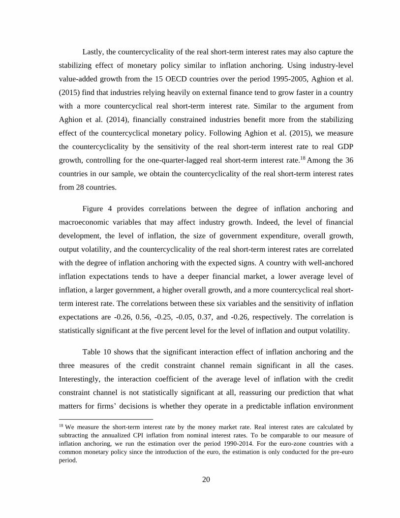
Lastly, the countercyclicality of the real short-term interest rates may also capture the

stabilizing effect of monetary policy similar to inflation anchoring. Using industry-level

value-added growth from the 15 OECD countries over the period 1995-2005, Aghion et al.

(2015) find that industries relying heavily on external finance tend to grow faster in a country

with a more countercyclical real short-term interest rate. Similar to the argument from

Aghion et al. (2014), financially constrained industries benefit more from the stabilizing

effect of the countercyclical monetary policy. Following Aghion et al. (2015), we measure

the countercyclicality by the sensitivity of the real short-term interest rate to real GDP

growth, controlling for the one-quarter-lagged real short-term interest rate.18 Among the 36

countries in our sample, we obtain the countercyclicality of the real short-term interest rates

from 28 countries.

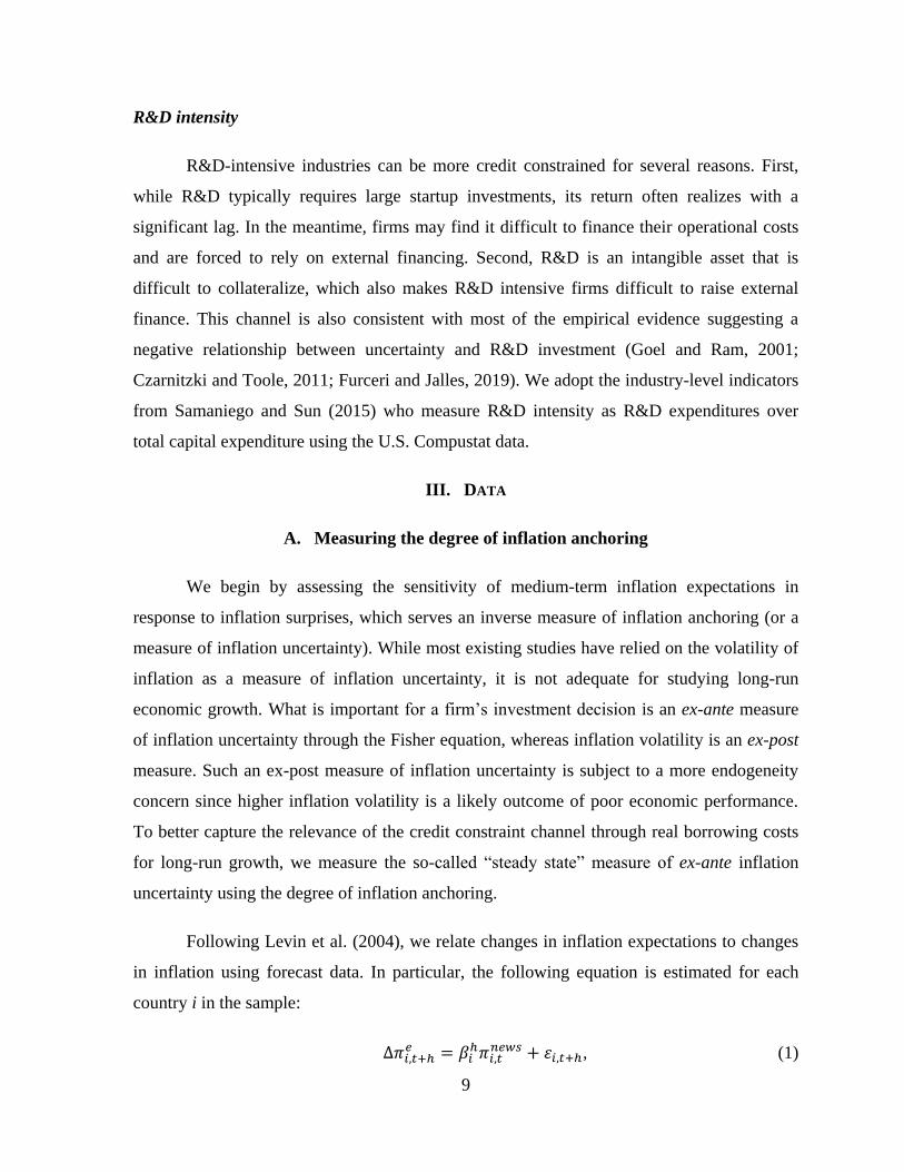
Figure 4 provides correlations between the degree of inflation anchoring and

macroeconomic variables that may affect industry growth. Indeed, the level of financial

development, the level of inflation, the size of government expenditure, overall growth,

output volatility, and the countercyclicality of the real short-term interest rates are correlated

with the degree of inflation anchoring with the expected signs. A country with well-anchored

inflation expectations tends to have a deeper financial market, a lower average level of

inflation, a larger government, a higher overall growth, and a more countercyclical real short-

term interest rate. The correlations between these six variables and the sensitivity of inflation

expectations are -0.26, 0.56, -0.25, -0.05, 0.37, and -0.26, respectively. The correlation is

statistically significant at the five percent level for the level of inflation and output volatility.

Table 10 shows that the significant interaction effect of inflation anchoring and the

three measures of the credit constraint channel remain significant in all the cases.

Interestingly, the interaction coefficient of the average level of inflation with the credit

constraint channel is not statistically significant at all, reassuring our prediction that what

matters for firms’ decisions is whether they operate in a predictable inflation environment

18 We measure the short-term interest rate by the money market rate. Real interest rates are calculated by

subtracting the annualized CPI inflation from nominal interest rates. To be comparable to our measure of

inflation anchoring, we run the estimation over the period 1990-2014. For the euro-zone countries with a

common monetary policy since the introduction of the euro, the estimation is only conducted for the pre-euro

period.

21

rather than a low-inflation enviornment.19 We take this as strong evidence to distinguish the

inflation uncertainty channel from the traditional inflation channel. Table 11 confirms that

our results survive even when controlling for the six factors simultaneously.20

Instrumental variables

We further address endogeneity concerns using an IV approach. Specifically, we use

the following set of indicators regarding the institutional quality of central banks as

instruments: (i) the central bank governor turnover index; (ii) the central bank independence

index; and (iii) the central bank transparency index. These indicators are largely exogenous

to our dependent variable of industry-level value-added growth, but they are strongly

correlated with the degree of inflation anchoring since inflation expectations tend to be better

anchored in a country with an independent and transparent central bank. We take the

indicators from the dataset constructed by Crowe and Meade (2007). Seeking for further

exogeneity of our instrumental variables, we use the values of the central bank governor

turnover index and the central bank independence index constructed from the institutional

data between 1980 and 1989 only, which does not overlap with our main sample period of

1990-2014. Among the 36 countries in our sample, the three indicators are available for 25

countries.

We proceed in two steps. In the first step, we regress the degree of inflation anchoring

on the three instrumental variables, controlling for the industry- and country-fixed effects.

The results of the first stage in Table 12 confirm that these three instruments can be

considered as “strong instruments”—that is, the Cragg-Donald Wald F-statistics are well

above the Stock and Yogo (2005) critical values for weak instruments in all cases. Hansen’s J

statistics for valid instruments are also reported in Table 12. In the second step, we re-

estimate equation (2) using the exogenous part of the degree of inflation anchoring driven by

these three instruments—that is, the fitted value of the first step. The results reported in Table

12 confirm that inflation anchoring enhances growth more for industries with heavier

19 While the countercyclicality of real short-term interest rates is only significant when interacting with R&D

intensity (Table 10), it does not necessarily contradict with Aghion et al. (2015), as our sample is substantially

larger than Aghion et al. (2015) in which 13 out of 15 countries are European countries.

20 To save space, we only report the coefficients of our ultimate interest.

22

external financial dependence and higher R&D intensity albeit with smaller effects than the

OLS case.

VI. CONCLUSIONS

Despite the famous claim that “Inflation is always and everywhere a monetary

phenomenon.” (Friedman, 1963), there has been the long-standing literature seeking a causal

relationship from inflation to long-run growth. By applying a difference-in-difference

approach to a large industry-level panel data including both advanced and emerging market

economies, this paper has examined how the effect of inflation anchoring on growth depends

on intrinsic characteristics capturing credit constraints.

We find that inflation anchoring fosters industry growth through the credit constraint

channel, as measured high external financial dependence and R&D intensity and low asset

tangibility. The fact that our results are robust to controlling for the interaction between

technological characteristics and a broad set of macroeconomic variables, such as financial

development, the level of inflation, size of government, overall economic growth, output

volatility, and monetary policy countercyclicality, assures that the credit constraint channel

of inflation uncertainty identified in the paper is unlikely confounded by other factors.

Since our finding can answer which kind of industries are expected to benefit more by

anchoring inflation expectations, it also sheds light on economy-wide gains from improving

the monetary policy framework. For example, improving a monetary policy framework to

anchor inflation expectations is expected to be more growth-friendly in an economy with a

larger share of credit constrained industries, or in periods where credit constraints are more

binding (such as during periods of recession).

23

References

Acemoglu, Daron, and Fabrizio Zilibotti. “Was Prometheus unbound by chance? Risk,

diversification, and growth.” Journal of Political Economy 105.4 (1997): 709-751.

Afonso, Antonio, and Davide Furceri. “Government size, composition, volatility and

economic growth.” European Journal of Political Economy 26.4 (2010): 517-532.

Aghion, Philippe, David Hemous, and Enisse Kharroubi (2014), “Cyclical fiscal policy,

credit constraints, and industry growth.” Journal of Monetary Economics 62, 41-58.

Aghion, Philippe, Emmanuel Farhi, and Enisse Kharroubi. “Liquidity and growth: the role of

counter-cyclical interest rates.” Working Paper (2015).

Aghion, Philippe, George-Marios Angeletos, Abhijit Banerjee, and Kalina Manova.

“Volatility and growth: Credit constraints and the composition of investment.” Journal of

Monetary Economics 57, no. 3 (2010): 246-265.

Arellano, Cristina, Yan Bai, and Patrick Kehoe. “Financial markets and fluctuations in

uncertainty.” Journal of Political Economy (forthcoming).

Baldwin, Carliss Y., and Richard S. Ruback. “Inflation, uncertainty, and investment.” Journal

of Finance 41.3 (1986): 657-668.

Ball, Laurence and Sandeep Mazumder. “Inflation Dynamics and the Great

Recession.” Brookings Papers on Economic Activity (2011): 337-405.

Barro, Robert J. “Inflation and growth.” Review-Federal Reserve Bank of Saint Louis 78

(1996): 153-169.

Berentsen, A., M. Rojas Breu, and S. Shi (2012): “Liquidity, innovation and growth.” Journal

of Monetary Economics, 59(8), 721-737.

Bernanke, Ben S., Thomas Laubach, Frederic S. Mishkin, and Adam S. Posen. “Inflation

targeting: lessons from the international experience” Princeton University Press, 1999.

Bernanke, Ben. “Irreversibility, uncertainty, and cyclical investment.” Quarterly Journal of

Economics, Vol. 97, No. 1, (1983), pp. 85-106.

Braun, Matias, and Borja Larrain (2005), “Finance and the business cycle: international,

inter‐industry evidence.” Journal of Finance 60(3), 1097-1128.

Choi, Sangyup, and Chansik Yoon. “Uncertainty, Financial Markets, and Monetary Policy

over the Last Century.” Yonsei University Working Paper. 2019.

24

Choi, Sangyup, Davide Furceri, and João Tovar Jalles. “Fiscal Stabilization and Growth:

Evidence from Industry-level Data for Advanced and Developing Economies.” IMF Working

Paper 17-198 (2017):1-48.

Choi, Sangyup, Davide Furceri, Yi Huang, and Prakash Loungani. “Aggregate uncertainty

and sectoral productivity growth: The role of credit constraints.” Journal of International

Money and Finance 88 (2018): 314-330.

Christiano, Lawrence J., Roberto Motto, and Massimo Rostagno. “Risk shocks.” American

Economic Review 104.1 (2014): 27-65.

Chu, A. C., and G. Cozzi (2014): “R&D and Economic Growth in a Cash-in-Advance

Economy,” International Economic Review, 55, 507-524.

Crowe, Christopher, and Ellen E. Meade. “The evolution of central bank governance around

the world.” Journal of Economic Perspectives 21.4 (2007): 69-90.

Czarnitzki, Dirk, and Andrew A. Toole (2011), “Patent protection, market uncertainty, and

R&D investment.” Review of Economics and Statistics 93(1), 147-159.

De Gregorio, Jose. “Inflation, taxation, and long-run growth.” Journal of Monetary

Economics 31.3 (1993): 271-298.

Debrun, Xavier, Jean Pisani-Ferry, and Andre Sapir. “Government Size and Output

Volatility: Should We Forsake Automatic Stabilization?” IMF Working Paper (2008): 1-53.

Dedola, Luca, and Francesco Lippi. “The monetary transmission mechanism: evidence from

the industries of five OECD countries.” European Economic Review 49.6 (2005): 1543-

1569.

Dell'Ariccia, Giovanni, Enrica Detragiache, and Raghuram Rajan. “The real effect of

banking crises.” Journal of Financial Intermediation 17.1 (2008): 89-112.

Dornbusch, Rudiger, and Jacob A. Frenkel. “Inflation and growth: alternative approaches.”

Journal of Money, Credit and Banking 5.1 (1973): 141-156.

Dotsey, Michael and Pierre-Daniel Sarte, “Inflation Uncertainty and Growth in a Cash-in-

Advance Economy.” Journal of Monetary Economics, 2000, 45 (3), 631–655.

Fatás, Antonio, and Ilian Mihov. “Government size and automatic stabilizers: international

and intranational evidence.” Journal of International Economics 55.1 (2001): 3-28.

Fischer, Stanley. “The role of macroeconomic factors in growth.” Journal of Monetary

Economics 32.3 (1993): 485-512.

25

Fischer, Stanley, and Franco Modigliani. “Towards an understanding of the real effects and

costs of inflation.” Review of World Economics 114.4 (1978): 810-833.

Friedman, Milton. “Inflation: Causes and consequences.” Asia Publishing House, 1963.

Furceri Davide and Jalles João Tovar (2019). “Fiscal counter-cyclicality and productive

investment: evidence from advanced economies.” The B.E. Journal of Macroeconomics, De

Gruyter, vol. 19(1), pages 1-15, January.

Goel, Rajeev K., and Rati Ram (2001), “Irreversibility of R&D investment and the adverse

effect of uncertainty: Evidence from the OECD countries.” Economics Letters 71(2), 287-

291.

Gonçalves, Carlos Eduardo S., and João M. Salles. “Inflation targeting in emerging

economies: What do the data say?” Journal of Development Economics 85.1-2 (2008): 312-

318.

Hart, Oliver, and John Moore (1994), “A theory of debt based on the inalienability of human

capital.” Quarterly Journal of Economics 109(4), 841-879.

Huizinga, John. “Inflation uncertainty, relative price uncertainty, and investment in US

manufacturing.” Journal of Money, Credit and Banking 25.3 (1993): 521-549.

Ilyina, Anna, and Roberto Samaniego. “Technology and financial development.” Journal of

Money, Credit and Banking 43.5 (2011): 899-921.

Imbs, Jean. “Growth and volatility.” Journal of Monetary Economics 54.7 (2007): 1848-

1862.

IMF (2016), “Global Disinflation in an Era of Constrained Monetary Policy”, World

Economic Outlook, Chapter 3, October 2016, International Monetary Fund.

Judson, Ruth, and Athanasios Orphanides. “Inflation, volatility and growth.” International

Finance 2.1 (1999): 117-138.

Levin, Andrew T., Fabio M. Natalucci, and Jeremy M. Piger. “The macroeconomic effects of

inflation targeting.” Review-Federal Reserve Bank of Saint Louis 86.4 (2004): 51-8.

Levine, Ross, and David Renelt. “A sensitivity analysis of cross-country growth

regressions.” American Economic Review (1992): 942-963.

López-Villavicencio, Antonia, and Valérie Mignon. “On the impact of inflation on output

growth: Does the level of inflation matter?” Journal of Macroeconomics 33.3 (2011): 455-

464.

https://ideas.repec.org/a/bpj/bejmac/v19y2019i1p15n8.html

https://ideas.repec.org/a/bpj/bejmac/v19y2019i1p15n8.html

https://ideas.repec.org/s/bpj/bejmac.html

26

Mishkin, Frederic S. “Inflation targeting in emerging-market countries.” American Economic

Review 90.2 (2000): 105-109.

Pindyck, Robert S. “Irreversibility, Uncertainty, and Investment.” Journal of Economic

Literature 29.3 (1991): 1110-1148.

Pindyck, Robert S. “Irreversible investment, capacity choice, and the value of the firm,”

American Economic Review, vol. 78(5), (1988), 969-85, December.

Rajan, Raghuram and Luigi Zingales (1998), “Financial Dependence and Growth.” American

Economic Review, 88 (3), 559-86

Ramey, Garey, and Valerie A. Ramey. “Cross-country evidence on the link between

volatility and growth." American Economic Review 85.5 (1995): 1138.

Samaniego, Roberto M., and Juliana Y. Sun. “Technology and contractions: Evidence from

manufacturing.” European Economic Review 79 (2015): 172-195.

Stock, James H., and Motohiro Yogo. “Testing for Weak Instruments in Linear IV

Regression.” Identification and Inference for Econometric Models: Essays in Honor of

Thomas Rothenberg (2005)

Tong, Hui, and Shang-Jin Wei (2011), “The composition matters: capital inflows and

liquidity crunch during a global economic crisis.” Review of Financial Studies 24(6), 2023-

2052.

Volcker, P., 1979, Statement before the Joint Economic Committee of the U.S. Congress.

October 17, 1979. Reprinted in Federal Reserve Bulletin 65 (11): 888–90.

27

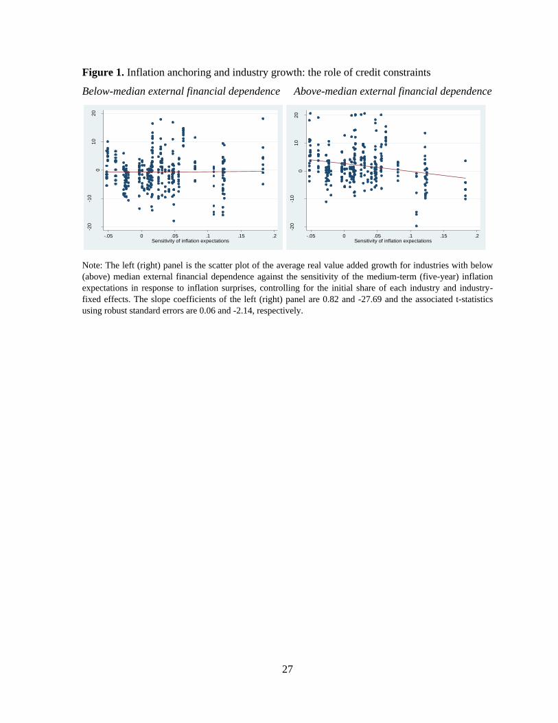
Figure 1. Inflation anchoring and industry growth: the role of credit constraints

Below-median external financial dependence Above-median external financial dependence

Note: The left (right) panel is the scatter plot of the average real value added growth for industries with below

(above) median external financial dependence against the sensitivity of the medium-term (five-year) inflation

expectations in response to inflation surprises, controlling for the initial share of each industry and industry-

fixed effects. The slope coefficients of the left (right) panel are 0.82 and -27.69 and the associated t-statistics

using robust standard errors are 0.06 and -2.14, respectively.

-20

-10

01

02

0

Ave

rag

e in

du

str

y v

alu

e a

dd

ed

gro

wth

-.05 0 .05 .1 .15 .2Sensitivity of inflation expectations

-20

-10

01

02

0

Ave

rag

e in

du

str

y v

alu

e a

dd

ed

gro

wth

-.05 0 .05 .1 .15 .2Sensitivity of inflation expectations

28

Figure 2. Change in inflation expectations and inflation shocks (percentage points)

Note: Data used in this figure are quarterly. In panels 1 and 2, the blue, red, and yellow lines denote changes in

expectations at 1-, 3-, and 5-year ahead in the furture, respectively. In panels 3 and 4, the blue lines denote the

median of inflation shocks, and shaded areas denote their interquartile ranges.

29

Figure 3. Sensitivity of the medium-term inflation expectations to inflation surprises

Note: The coefficients from estimating equation (1) using 5-year ahead inflation expectations. * indicates that

the estimated coefficient is statistically significant at the 10% level.

*

*

* **

*

*

* *

-0.1

-0.05

0

0.05

0.1

0.15

0.2

Au

stra

lia

Bra

zil

Can

ada

Ch

ile

Ch

ina

Co

lom

bia

Cze

ch R

epu

bli

c

Est

on

ia

Fra

nce

Ger

man

y

Ho

ng

Ko

ng

Hu

ng

ary

India

Indo

nes

ia

Ital

y

Japan

Ko

rea

Lat

via

Lit

huan

ia

*

*

*

-0.1

-0.05

0

0.05

0.1

0.15

0.2

Mal

aysi

a

Mex

ico

Net

her

land

s

New

Zel

and

No

rway

Po

lan

d

Ro

man

ia

Ru

ssia

Sin

gap

ore

Slo

vak

ia

Slo

ven

ia

Sp

ain

Sw

eden

Sw

itze

rlan

d

Tai

wan

Turk

ey

Uk

rain

e

Un

ited

Kin

gd

om

30

Figure 4. Correlations between the sensitivity of inflation expectations and other factors

Note: The correlations between the sensitivity of inflation expectations and private credit to GDP, CPI inflation,

general government expenditure to GDP, real GDP growth, volatility of real GDP growth, and real interest rate

countercyclicality are -0.26 (0.15), 0.56 (0.01), -0.25 (0.14), -0.05 (0.80), 0.37 (0.03), -0.26 (0.25), respectively.

The numbers in parantheses are associated p-values.

-.05

0

.05

.1.1

5.2

Se

nsitiv

ity o

f th

e m

ed

ium

-te

rm infla

tion

expe

cta

tion

s

0 50 100 150 200Average private credit to GDP

-.05

0

.05

.1.1

5.2

Se

nsitiv

ity o

f th

e m

ed

ium

-te

rm infla

tion

expe

cta

tion

s

0 10 20 30 40 50Average CPI inflation

-.05

0

.05

.1.1

5.2

Se

nsitiv

ity o

f th

e m

ed

ium

-te

rm infla

tion

expe

cta

tion

s

20 30 40 50 60Average general government expenditure to GDP

-.05

0

.05

.1.1

5.2

Sen

sitiv

ity o

f th

e m

ediu

m-t

erm

infla

tion

expe

cta

tion

s

0 2 4 6 8Average real GDP growth

-.05

0

.05

.1.1

5.2

Sen

sitiv

ity o

f th

e m

ediu

m-t

erm

infla

tion

expe

cta

tion

s

-.5 0 .5 1Real interest rate countercyclicality

31

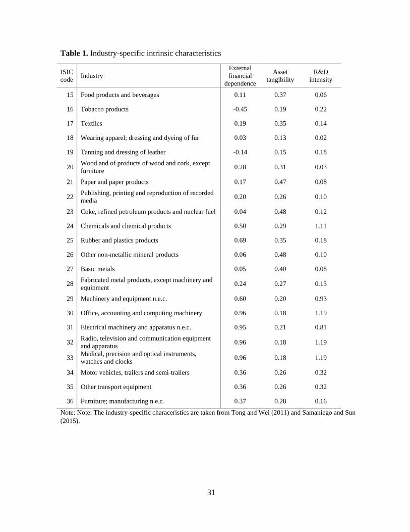
Table 1. Industry-specific intrinsic characteristics

ISIC

code Industry

External

financial

dependence

Asset

tangibility

R&D

intensity

15 Food products and beverages 0.11 0.37 0.06

16 Tobacco products -0.45 0.19 0.22

17 Textiles 0.19 0.35 0.14

18 Wearing apparel; dressing and dyeing of fur 0.03 0.13 0.02

19 Tanning and dressing of leather -0.14 0.15 0.18

20 Wood and of products of wood and cork, except

furniture 0.28 0.31 0.03

21 Paper and paper products 0.17 0.47 0.08

22 Publishing, printing and reproduction of recorded

media 0.20 0.26 0.10

23 Coke, refined petroleum products and nuclear fuel 0.04 0.48 0.12

24 Chemicals and chemical products 0.50 0.29 1.11

25 Rubber and plastics products 0.69 0.35 0.18

26 Other non-metallic mineral products 0.06 0.48 0.10

27 Basic metals 0.05 0.40 0.08

28 Fabricated metal products, except machinery and

equipment 0.24 0.27 0.15

29 Machinery and equipment n.e.c. 0.60 0.20 0.93

30 Office, accounting and computing machinery 0.96 0.18 1.19

31 Electrical machinery and apparatus n.e.c. 0.95 0.21 0.81

32 Radio, television and communication equipment

and apparatus 0.96 0.18 1.19

33 Medical, precision and optical instruments,

watches and clocks 0.96 0.18 1.19

34 Motor vehicles, trailers and semi-trailers 0.36 0.26 0.32

35 Other transport equipment 0.36 0.26 0.32

36 Furniture; manufacturing n.e.c. 0.37 0.28 0.16

Note: Note: The industry-specific characeristics are taken from Tong and Wei (2011) and Samaniego and Sun

(2015).

32

Table 2. Correlation matrix of industry-specific characteristics

External financial

dependence Asset tangibility R&D intensity

External financial

dependence 1

Asset tangibility -0.27 1

R&D intensity 0.73 -0.40 1

Note: The industry-specific characeristics are taken from Tong and Wei (2011) and Samaniego and Sun (2015).

Table 3. Country coverage and the number of industries used in the analysis

Country Number of

industries Country

Number of

industries

Australia 11 Lithuania 18

Brazil 21 Malaysia 18

Canada 22 Mexico 16

Chile 12 Netherlands 20

China 18 New Zealand 5

Colombia 18 Norway 21

Czech Republic 18 Poland 22

Estonia 19 Romania 18

France 21 Russia 18

Germany 20 Singapore 22

Hong Kong 17 Slovakia 20

Hungary 21 Slovenia 16

India 21 Spain 22

Indonesia 20 Sweden 22

Italy 22 Switzerland 11

Japan 20 Taiwan 16

Korea 22 Turkey 22

Latvia 18 United Kingdom 20

Note: Only industries with more than 15 years of consecutive data are included in the analysis.

33

Table 4. The effect of inflation anchoring on industry growth: baseline

Explanatory variable (I) (II) (III)

Initial share -0.959*** -0.904*** -0.952***

(0.287) (0.300) (0.291)


*Inflation anchoring

-39.860***

(11.911)

Asset tangibility


66.067**

(27.415)

R&D intensity


-26.960***

(8.512)

Magnitude of differential effects -1.24 0.61 -1.12

Observations 668 668 668

R-squared 0.6 0.59 0.59

Note: The dependent variable is the average annual growth rate in real value added from 1990 to 2014 for each

industry-country pair. Estimates based on equation (2). t-statistics based on clustered standard errors at the

country level are reported in parenthesis. *, **, *** denote significance at 10, 5 and 1 percent, respectively.

Differential effects computed as the change in inflation anchoring from the 75th percent to the 25th percentile of

the cross-country distribution between a sector with high external financial dependence (at the 75th percentile of

the distribution) and a sector with low external financial dependence (at the 25th percentile of the distribution).

Table 5. The effect of inflation anchoring on industry growth: using gross output


Initial share -0.798*** -0.761*** -0.791***

(0.259) (0.266) (0.266)



-35.787**

(15.321)

Asset tangibility


36.717

(33.957)

R&D intensity


-23.030***

(7.550)

Magnitude of differential effects -1.18 0.34 0.96


R-squared 0.61 0.60 0.60

Note: The dependent variable is the average annual growth rate in real gross output from 1990 to 2014 for each






34

Table 6. The effect of inflation anchoring on industry growth: 1990-2007


Initial share -1.123*** -1.176*** -1.121***

(0.393) (0.412) (0.399)



-46.607***

(14.832)

Asset tangibility


62.451*

(32.856)

R&D intensity


-30.172***

(9.586)



R-squared 0.57 0.56 0.56







Table 7. The effect of inflation anchoring on industry growth: excluding euro-area countries


Initial share -1.086*** -1.031*** -1.097***

(0.297) (0.308) (0.292)



-37.798***

(11.330)

Asset tangibility


56.406**

(26.106)

R&D intensity


-30.519***

(9.283)



R-squared 0.66 0.65 0.59


industry-country pair after dropping 10 euro-area countries. Estimates based on equation (2). t-statistics based

on clustered standard errors at the country level are reported in parenthesis. *, **, *** denote significance at 10,

5 and 1 percent, respectively. Differential effects computed as the change in inflation anchoring from the 75th

percent to the 25th percentile of the cross-country distribution between a sector with high external financial

dependence (at the 75th percentile of the distribution) and a sector with low external financial dependence (at the

25th percentile of the distribution).

35

Table 8. The effect of inflation anchoring on industry growth: using WLS


Initial share -0.927** -0.794* -0.913**

(0.362) (0.409) (0.375)



-48.005***

(11.072)

Asset tangibility


84.018***

(19.455)

R&D intensity


-33.032***

(10.206)



R-squared 0.60 0.60 0.60







36

Table 9. The effect of inflation anchoring on industry growth: alternative measure of the degree of inflation anchoring

Short-term expectations (one year) Alternative inflation shocks Absolute sensitivity

Explanatory variable (I) (II) (III) (IV) (V) (VI) (VII) (VIII) (IX)

Initial share -0.959*** -0.924*** -0.953*** -0.983*** -0.936*** -0.956*** -0.960*** -0.887*** -0.932***

(0.308) (0.310) (0.308) (0.301) (0.303) (0.305) (0.282) (0.298) (0.294)



-3.533*** -15.540*** -60.016***

(1.189) (5.406) (13.118)

Asset tangibility


7.435*** 13.176 108.864***

(2.389) (15.912) (29.334)

R&D intensity


-2.417** -13.005*** -38.665***

(1.128) (4.131) (11.166)

Magnitude of differential

effects -0.33 0.21 -0.30 -0.85 0.21 -0.94 -1.28 0.68 -1.09

Observations 668 668 668 668 668 668 668 668 668

R-squared 0.59 0.59 0.59 0.60 0.60 0.60 0.59 0.59 0.59

Note: The dependent variable is the average annual growth rate in real value added from 1990 to 2014 for each industry-country pair. Estimates based on

equation (2). t-statistics based on clustered standard errors at the country level are reported in parenthesis. *, **, *** denote significance at 10, 5 and 1 percent,

respectively. Differential effects computed as the change in inflation anchoring from the 75th percent to the 25th percentile of the cross-country distribution

between a sector with high external financial dependence (at the 75th percentile of the distribution) and a sector with low external financial dependence (at the


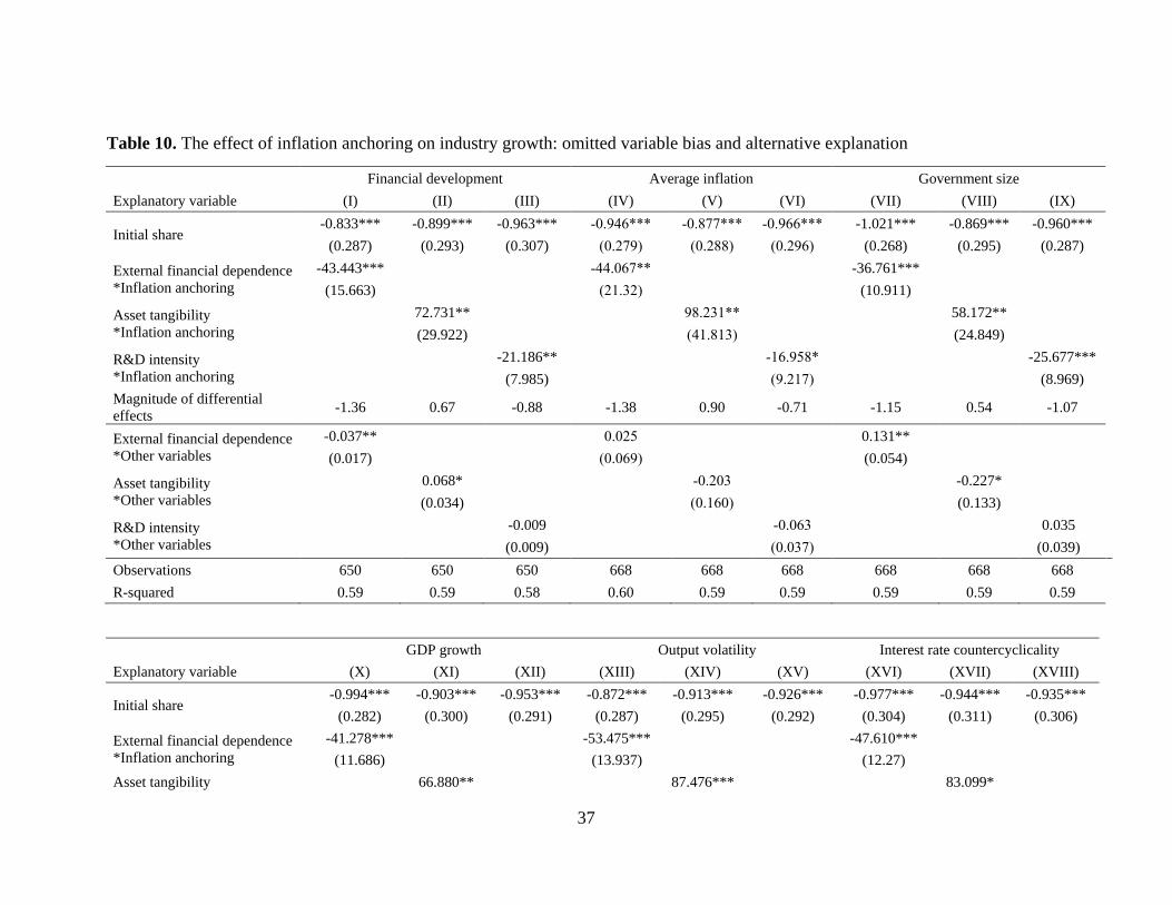
37

Table 10. The effect of inflation anchoring on industry growth: omitted variable bias and alternative explanation

Financial development Average inflation Government size

Explanatory variable (I) (II) (III) (IV) (V) (VI) (VII) (VIII) (IX)

Initial share -0.833*** -0.899*** -0.963*** -0.946*** -0.877*** -0.966*** -1.021*** -0.869*** -0.960***

(0.287) (0.293) (0.307) (0.279) (0.288) (0.296) (0.268) (0.295) (0.287)



-43.443*** -44.067** -36.761***

(15.663) (21.32) (10.911)

Asset tangibility


72.731** 98.231** 58.172**

(29.922) (41.813) (24.849)

R&D intensity


-21.186** -16.958* -25.677***

(7.985) (9.217) (8.969)


effects -1.36 0.67 -0.88 -1.38 0.90 -0.71 -1.15 0.54 -1.07


*Other variables

-0.037** 0.025 0.131**

(0.017) (0.069) (0.054)

Asset tangibility

*Other variables

0.068* -0.203 -0.227*

(0.034) (0.160) (0.133)

R&D intensity

*Other variables

-0.009 -0.063 0.035

(0.009) (0.037) (0.039)

Observations 650 650 650 668 668 668 668 668 668

R-squared 0.59 0.59 0.58 0.60 0.59 0.59 0.59 0.59 0.59

GDP growth Output volatility Interest rate countercyclicality

Explanatory variable (X) (XI) (XII) (XIII) (XIV) (XV) (XVI) (XVII) (XVIII)

Initial share -0.994*** -0.903*** -0.953*** -0.872*** -0.913*** -0.926*** -0.977*** -0.944*** -0.935***

(0.282) (0.300) (0.291) (0.287) (0.295) (0.292) (0.304) (0.311) (0.306)



-41.278*** -53.475*** -47.610***

(11.686) (13.937) (12.27)

Asset tangibility 66.880** 87.476*** 83.099*

38

*Inflation anchoring (27.773) (31.701) (46.047)

R&D intensity


-27.224*** -31.097*** -32.706*** (8.398) (8.601) (7.651)


effects -1.29 0.61 -1.13 -1.67 0.80 -1.29 -1.49 0.76 -1.36


*Other variables

-0.340 1.187*** 0.875

(0.208) (0.388) (1.301)

Asset tangibility

*Other variables

0.286 -1.919* 3.633

(0.689) (1.091) (5.515)

R&D intensity

*Other variables

-0.072 0.373 1.158* (0.171) (0.263) (0.670)

Observations 668 668 668 668 668 668 415 415 415

R-squared 0.59 0.59 0.59 0.60 0.59 0.59 0.56 0.56 0.56

Note: The dependent variable is the average annual growth rate in real value added from 1990 to 2014 for each industry-country pair. Estimates based on

equation (2). t-statistics based on clustered standard errors at the country level are reported in parenthesis. *, **, *** denote significance at 10, 5 and 1 percent,

respectively. Differential effects computed as the change in inflation anchoring from the 75th percent to the 25th percentile of the cross-country distribution

between a sector with high external financial dependence (at the 75th percentile of the distribution) and a sector with low external financial dependence (at the


39

Table 11. The effect of inflation anchoring on industry growth: controlling for all factors


Initial share -0.851*** -0.939*** -0.863***

(0.279) (0.298) (0.304)



-47.607***

(13.511)

Asset tangibility


116.514*

(59.644)

R&D intensity


-24.762**

(10.026)



R-squared 0.57 0.59 0.59







Table 12. The effect of inflation anchoring on industry growth: IV regression


Initial share -0.972*** -0.970*** -0.962***

(0.277) (0.295) (0.275)



-31.289**

(13.321)

Asset tangibility


44.842

(83.625)

R&D intensity


-23.171*

(13.697)


Cragg-Donald Wald F-statistic 61.202 54.172 57.908

Stock-Yogo weak identification

test 5% critical values 13.91 13.91 13.91

Hansen J-statistic p-value 0.118 0.914 0.187


R-squared 0.42 0.39 0.42







40

Appendix

Table A.1. Degree of inflation anchoring

(I) (II) (III) (IV) (V)

Country 1-year

coef

1-year

s.e.

2-year

coef

2-year

s.e.

3-year

coef

3-year

s.e.

4-year

coef

4-year

s.e.

5-year

coef

5-year

s.e.

Argentina 0.756 0.090 0.554 0.079 0.360 0.068 0.234 0.030 0.200 0.026

Australia 0.085 0.042 0.009 0.018 0.005 0.017 0.020 0.016 0.036 0.026

Brazil 0.430 0.114 0.299 0.104 0.232 0.098 0.138 0.060 0.122 0.052

Canada 0.040 0.043 0.020 0.022 0.002 0.013 -0.015 0.013 -0.027 0.014

Chile 0.117 0.028 0.052 0.021 0.047 0.026 0.049 0.026 0.057 0.032

China 0.128 0.022 0.089 0.027 0.078 0.019 0.069 0.017 0.063 0.014

Colombia 0.175 0.068 0.132 0.064 0.094 0.044 0.051 0.052 0.081 0.031

Croatia 0.037 0.055 0.013 0.036 -0.021 0.013 -0.002 0.027 -0.013 0.026

Czech Republic 0.170 0.054 0.090 0.029 0.057 0.028 0.056 0.034 0.056 0.024

Estonia 0.295 0.081 0.098 0.043 0.029 0.034 0.005 0.040 0.047 0.031

Euro area 0.141 0.072 0.053 0.028 0.028 0.016 0.014 0.017 0.025 0.010

France 0.073 0.038 0.018 0.017 -0.016 0.015 0.009 0.017 0.009 0.014

Germany 0.068 0.050 0.029 0.023 0.006 0.018 -0.008 0.023 -0.023 0.015

Hong Kong 0.238 0.083 0.122 0.090 0.107 0.055 0.100 0.036 0.109 0.048

Hungary 0.179 0.103 0.062 0.039 0.035 0.027 0.026 0.020 0.026 0.018

India -0.014 0.021 -0.029 0.037 -0.017 0.033 -0.042 0.036 -0.051 0.037

Indonesia 0.351 0.082 0.124 0.014 0.058 0.011 0.024 0.009 0.017 0.004

Italy 0.197 0.042 0.040 0.030 -0.006 0.030 0.034 0.030 -0.003 0.034

Japan 0.106 0.050 0.061 0.035 0.048 0.028 0.056 0.027 0.041 0.028

Korea 0.129 0.029 0.016 0.031 0.005 0.013 0.007 0.011 -0.039 0.015

Latvia 0.349 0.168 0.193 0.046 0.066 0.028 0.039 0.014 0.015 0.013

41

Lithuania 0.250 0.145 0.137 0.091 0.082 0.055 0.068 0.098 0.062 0.072

Malaysia 0.148 0.058 0.042 0.021 0.018 0.023 0.009 0.029 0.029 0.035

Mexico 0.427 0.131 0.270 0.089 0.226 0.067 0.192 0.050 0.183 0.056

Netherlands 0.037 0.045 0.026 0.024 0.017 0.025 0.015 0.024 0.047 0.039

New Zealand 0.054 0.050 -0.012 0.017 -0.001 0.013 0.015 0.013 0.004 0.011

Norway -0.003 0.035 -0.006 0.011 0.003 0.010 0.002 0.008 0.001 0.007

Peru 0.131 0.045 0.061 0.057 0.031 0.040 0.008 0.035 0.023 0.041

Philippines 0.045 0.043 0.035 0.079 0.007 0.077 0.003 0.079 0.055 0.070

Poland 0.113 0.050 0.051 0.032 0.041 0.029 0.042 0.032 0.049 0.034

Romania 0.299 0.132 0.200 0.110 0.170 0.082 0.168 0.065 0.122 0.089

Russia 1.536 0.981 0.384 0.188 0.252 0.109 0.210 0.084 0.125 0.063

Singapore 0.169 0.036 0.079 0.024 0.041 0.024 0.013 0.019 0.016 0.023

Slovak Republic 0.103 0.029 -0.019 0.026 -0.042 0.022 -0.045 0.024 -0.052 0.028

Slovenia 0.054 0.114 0.024 0.047 0.000 0.035 -0.018 0.021 -0.023 0.021

Spain 0.124 0.045 0.043 0.023 0.027 0.015 0.032 0.015 0.014 0.015

Sweden 0.108 0.053 0.049 0.027 0.037 0.018 -0.007 0.014 0.011 0.016

Switzerland 0.139 0.042 0.103 0.035 0.031 0.021 0.000 0.024 -0.020 0.025

Taiwan 0.045 0.034 0.006 0.018 0.010 0.015 0.010 0.018 -0.001 0.017

Thailand 0.166 0.067 0.113 0.066 0.055 0.060 0.006 0.017 0.021 0.011

Turkey 0.284 0.092 0.149 0.078 0.119 0.081 0.054 0.037 0.031 0.026

Ukraine 0.177 0.051 0.051 0.025 0.026 0.020 0.015 0.016 0.013 0.014

United Kingdom 0.137 0.081 0.049 0.022 0.049 0.023 -0.017 0.033 -0.025 0.033

United States 0.067 0.028 0.013 0.010 0.010 0.011 0.003 0.011 -0.004 0.011

Venezuela 0.343 0.103 0.007 0.145 0.023 0.144 -0.008 0.104 -0.042 0.099

Note: This table summarizes the results from estimating equation (1) country-by-country using inflation expectations at various horizons.

42

Table A.2. Industry classification: INDSTAT2 vs. INDSTAT3

INDSTAT2 INDSTAT3

ISIC Industry ISIC Industry

15 Food products and beverages 311 Food

16 Tobacco products 313 Beverages

17 Textiles 314 Tobacco

18 Wearing apparel; dressing and dyeing of fur 321 Textiles

19 Tanning and dressing of leather 322 Apparel

20 Wood and of products of wood and cork, except

furniture 323 Leather

21 Paper and paper products 324 Footwear

22 Publishing, printing and reproduction of

recorded media 331 Wood products

23 Coke, refined petroleum products and nuclear

fuel 332 Furniture, except metal

24 Chemicals and chemical products 341 Paper and products

25 Rubber and plastics products 342 Printing and publishing

26 Other non-metallic mineral products 351 Industrial chemicals

27 Basic metals 352 Other chemicals

28 Fabricated metal products, except machinery

and equipment 353 Petroleum refineries

29 Machinery and equipment n.e.c. 354 Misc. pet. And coal products

30 Office, accounting and computing machinery 355 Rubber products

31 Electrical machinery and apparatus n.e.c. 356 Plastic products

32 Radio, television and communication

equipment and apparatus 361 Pottery, china, earthenware

33 Medical, precision and optical instruments,

watches and clocks 362 Glass and products

34 Motor vehicles, trailers and semi-trailers 369 Other nonmetallic mineral products

35 Other transport equipment 371 Iron and steel

36 Furniture; manufacturing n.e.c. 372 Nonferrous metals

381 Fabricated metal products

382 Machinery, except electrical

383 Machinery, electric

384 Transport equipment

385 Prof. and sci. equip.

390 Other manufactured products

Source: Unido.

43

Table A.3. The effect of inflation anchoring on industry growth: standard errors clustered at

the industry-level


Log of initial share -0.959*** -0.904*** -0.952***

(0.287) (0.300) (0.291)



-39.860***

(10.952)

Asset tangibility


66.067*

(38.183)

R&D intensity


-26.960**

(11.190)



R-squared 0.60 0.59 0.59


industry-country pair. Initial share in manufacturing value added is the ratio of industry-level real value added

to total real manufacturing value added in the initial period. t-statistics based on clustered standard errors at the

industry level are reported in parenthesis. *, **, *** denote significance at 10, 5 and 1 percent, respectively.

inflation anchoring, real borrowing costs, and growth

Documents