infield re-injection strategies in olkaria, kenya… · geothermal training programme reports 2004...

GEOTHERMAL TRAINING PROGRAMME Reports 2004 Orkustofnun, Grensásvegur 9, Number 12 IS-108 Reykjavík, Iceland

239

INFIELD RE-INJECTION STRATEGIES IN OLKARIA, KENYA, BASED ON TRACER STUDIES AND NUMERICAL MODELLING

Godwin M. Mwawongo Kenya Electricity Generating Company Ltd. – KenGen

Olkaria Geothermal Project P.O. Box 785, Naivasha

KENYA [email protected]

ABSTRACT

In two-phase geothermal reservoirs, efficient heat mining process can be achieved by injecting deep into the liquid zone at an optimum rate that will maintain the boiling level at the same depth while producing from a shallower level. Optimum resource utilization in Olkaria East production field requires intermittent infield re-injection around the central part of the field followed by a temperature recovery period. Numerical methods can be used to model fluid flowpaths in fractured two-phase reservoirs. Tracer tests can be used to calibrate such models. Reservoir cooling under varied injection scenarios can then be predicted. In this report, a two-dimensional fracture model analysis, resulting from tracer and injection tests conducted in well OW-12, is presented. Wells OW-12 and OW-19 are connected at depth by an 800 m deep by 400 m wide and 1 m thick fracture. Cold and hot re-injection into well OW-12 at 8 kg/s will cool the formation by 55°C and 25°C, respectively, in twenty years. Cold injection can be done for 11/2 years followed by a similar recovery period.

1. INTRODUCTION Kenya is located in East Africa where the eastern arm of the Great African Rift virtually splits the landmass into two. Fourteen geothermal prospects have been identified within the Kenyan Rift Valley starting from Barrier in the north to Lake Magadi in the south. Olkaria geothermal field is situated about 120 km northwest of the capital, Nairobi and 10 km south of Lake Naivasha (Figure 1). Early scientific work in Olkaria was carried out between 1955 and 1959 when two exploration wells X-1 and X-2 were drilled but failed to discharge. In the mid 1960´s, a reconnaissance geophysical survey was carried out in the Rift Valley between Lake Bogoria and Olkaria. This identified several low-resistivity areas suitable for geothermal prospecting, Olkaria being one of them. In 1970, a geothermal prospecting programme funded by the UNDP carried out extensive geological, geophysical, hydrogeological and geochemical surveys while tests were performed on X-2. Well X-2 was discharged. Results from these studies combined with economical considerations identified Olkaria as the best candidate for further exploration work (KPC, 1994).

Mwawongo Report 12

240

Exploration drilling commenced in 1973 and by 1976, six wells had been drilled in Olkaria. A 45 MWe plant was installed between 1981 and 1986 (KPC, 1994). Further exploration work led to the discovery of Olkaria Northeast, South, Northwest and the Domes which all form the Greater Olkaria geothermal area. A 70 MWe unit was commissioned in December 2003 in the Northeast sector while 13 MWe are generated from the Southwest sector by a private developer. Direct utilization of geothermal heat for fumigation is done at the Olkaria Northwest site by a private developer. The current near 130 MWe generation in Olkaria results in considerable flowrates of geothermal brines that need to be disposed of. Re-injection is the process of returning separated brine back into reservoirs. The objective is to stabilise the reservoir pressure as well as provide an environmentally friendly way of disposal. Peripheral re-injection can also act as a barrier to cold inflow into the productive well field. Re-injection can enhance heat mining efficiency and therefore increase the life of the reservoir as well as reduce the number of make-up wells required.

As a part of Olkaria reservoir management programme, a long term injection experiment was conducted in the East production field from July 1996 to September 1997 using cold water from Lake Naivasha. The objective was to study fluid flowpaths in the reservoir. A 500 kg slug of flourescein was also injected into well OW-12 and monitored for in all production wells. Results obtained indicated hydrological connection between well OW-12 and production wells OW-15, OW-16, OW-18 and OW-19 (Ofwona, 2002). Increased steam and water production was observed in the affected wells. Analysis and modelling of the data obtained is the subject of this report. After introducing Olkaria in general, a special chapter is devoted to the data collected in the 1996 - 1997 injection and tracer tests. Thermal degradation of the flourescein tracer applied is discussed and some corrections made. One-dimensional tracer flow models are defined by inverse numerical simulation. Some basic geometric properties of flowpaths connecting injection and production wells are defined. With these estimations at hand, the analysis proceeds into a two-dimensional (2-D) numerical reservoir model study where TOUGH2 simulator is applied. These numerical models not only matched selected tracer recovery curves but also estimate temperature distribution within fractures that connect injection and production wells. The calibrated 2-D fracture models are finally used to predict thermal efficiency of several injection scenarios where factors such as injection rates, permeability, well separation and temperatures are varied.

FIGURE 1: Location of geothermal prospects in Kenya

Report 12 Mwawongo

241

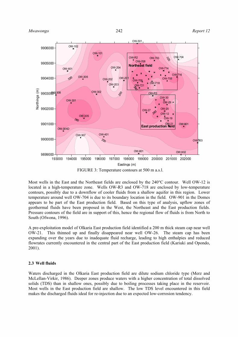
2. OLKARIA GEOTHERMAL FIELD 2.1 Geology Structurally the Rift Valley can be divided into the Northern, Central and Southern parts. Olkaria is in the Central part which stretches from Lake Bogoria in the north to Lake Naivasha in the south. Here the East African Rift trends NNW-SSE and has an elevation in excess of 1800 m (Figure 2). The rift floor is characterized by numerous volcanic centres, dense fracturing and up doming (KPC, 1994). The geothermal field is associated with the Olkaria volcanic centre. The reservoir appears bounded by accuate faults forming a ring structure (Naylor, 1972). An impermeable 400-700 m thick layer of mainly basalts and trachyte form a reservoir cap rock (Kariuki and Ouma, 2002). The reservoir rocks consist of successive strata of rhyolite, trachyte and basalts. The Olkaria rhyolite has been defined as a contributor of lateral permeability in the East production field. Most wells in this field have feed zones in this layer. Fractures also contribute to well discharge (Merz and McLellan-Virkir, 1981). The hydrology of the reservoir is controlled by the Olkaria fault. The fault is fed with fluids from the east mainly of sodium chloride type, while fluids with high bicarbonate level flow from the west along the same fault (Bödvarsson and Pruess, 1987). The two flows mix in the Central sector where the mixture is conducted southwards along the Ol Butot fault (Figure 2). 2.2 Conceptual reservoir model Figure 3 presents temperature contours at 500 m above sea level (1000-1500 m depth). These indicate high temperatures (>280°C) in the north of the East production field. Much lower temperatures (< 220°C) are encountered in the central sector around well OW-201 through to OW-204. The N-S trending Ol Butot fault, a conductor of cooler fluids has been associated with this region (Figures 2 and 3).

FIGURE 2: Structural map and well locations in Olkaria SWF (Southwest field), NEF (Northeast field) and EPF (East production field)

Mwawongo Report 12

242

Most wells in the East and the Northeast fields are enclosed by the 240°C contour. Well OW-12 is located in a high-temperature zone. Wells OW-R3 and OW-718 are enclosed by low-temperature contours, possibly due to a downflow of cooler fluids from a shallow aquifer in this region. Lower temperature around well OW-704 is due to its boundary location in the field. OW-901 in the Domes appears to be part of the East production field. Based on this type of analysis, upflow zones of geothermal fluids have been proposed in the West, the Northeast and the East production fields. Pressure contours of the field are in support of this, hence the regional flow of fluids is from North to South (Ofwona, 1996). A pre-exploitation model of Olkaria East production field identified a 200 m thick steam cap near well OW-21. This thinned up and finally disappeared near well OW-26. The steam cap has been expanding over the years due to inadequate fluid recharge, leading to high enthalpies and reduced flowrates currently encountered in the central part of the East production field (Kariuki and Opondo, 2001). 2.3 Well fluids Waters discharged in the Olkaria East production field are dilute sodium chloride type (Merz and McLellan-Virkir, 1986). Deeper zones produce waters with a higher concentration of total dissolved solids (TDS) than in shallow ones, possibly due to boiling processes taking place in the reservoir. Most wells in the East production field are shallow. The low TDS level encountered in this field makes the discharged fluids ideal for re-injection due to an expected low-corrosion tendency.

193000 194000 195000 196000 197000 198000 199000 200000 201000 202000Eastings (m)

9899000

9900000

9901000

9902000

9903000

9904000

9905000

9906000

Nor

thin

gs (m

)

OW-101

OW-102

OW-19

OW-201OW-202

OW-204

OW-27

OW-29

OW-30OW-301

OW-302

OW-304D

OW-305

OW-306

OW-307 OW-401

OW-501

OW-601

OW-703 OW-704

OW-705

OW-708

OW-709

OW-714

OW-716

OW-718OW-721

OW-R2

OW-203

OW-308

OW-21

OW-20

OW-R3

OW-801

OW-901

OW-902

OW-903

OW-12

East production field

Northeast field

FIGURE 3: Temperature contours at 500 m a.s.l.

Report 12 Mwawongo

243

3. AN OVERVIEW OF OLKARIA RE-INJECTION ACTIVITIES Historically speaking, re-injection started as a brine disposal method but now it has become an essential part of reservoir management worldwide. Only a small part of the thermal energy in place in geothermal reservoirs can be recovered without re-injection if the outer reservoir boundaries are nearly tight and, thus, provide little pressure support. Peripheral injection locations commonly recover a third of the re-injected fluids. Re-injection within production areas result in a higher ratio of fluid recovery (Stefánsson, 1997, Axelsson, 2004). Olkaria has relatively low permeability but high rock temperatures. In such fields, re-injection appears most feasible for mining the heat inherent in the reservoir rocks. Previous simulation studies have consequently identified re-injection as a requirement for optimum field operation in Olkaria (Bödvarsson and Pruess, 1984, 1987). Optimal development and management of geothermal resources requires a good knowledge of the hydrological characteristics of the reservoir. Tracer tests are a powerful tool used to identify flowpaths in geothermal reservoirs. The tests have been extensively used in studying groundwater hydrology, pollution as well as underground nuclear waste disposal. The results have also been used to study and quantify fluid flowpaths (Axelsson, 2004). In geothermal reservoirs pressure, chemical and thermal response to injection occurs in the listed order. Chemical fronts travel an order of magnitude faster than thermal fronts. Tracer tests can therefore be used to predict thermal breakthrough long before they occur (Axelsson, 2004). Reservoir parameters that govern flow in geothermal reservoirs can also be estimated by tracer data analysis (Shook and Renner, 2002). Re-injection in the Northeast field is at present both peripheral and infield. Production wells are grouped as shown in Figure 4 for re-injection at wells R-2 (peripheral), R-3 (infield), OW-708

FIGURE 4: Well locations in Olkaria East and Northeast fields; shaded polygons present groups of wells connected to the same re-injection well

Mwawongo Report 12

244

(infield) and OW-703 (infield). The well grouping was done based on re-injection well capacity (Ouma, 2003). Brine overflow from one sector of the field to the other has been allowed for in the design of the injection system. This has an advantage of flexibility, thereby minimising possible negative effects of re-injection. Condensate from the Northeast plant is pumped to wells OW-201 and OW-204 in Olkaria Central field. From the conceptual model of Olkaria, this area is associated with Ol Butot fault which conducts cooler fluids southwards. The area also acts as a buffer zone between the fields in the East and the West of Olkaria hill. Well OW-R3 is located in the buffer zone of Olkaria Northeast and the East production field with the intension of stabilising reservoir pressure in the East production field. Thermal breakthrough is the decline in enthalpy, not associated with an increase in mass flowrate, hence due to thermal effects rather than pressure effects (Bödvarsson and Stefánsson, 1987). In the East production field, hot re-injection into well OW-3 has been ongoing since 1995 resulting in improved well performance in wells OW-2, OW-7, OW-8 and OW-11. Thermal breakthrough has not occurred in them. In Olkaria, re-injection has resulted in increased cyclicity in some wells while others have been stabilised (Mwawongo, 2002). Wells OW-18 and OW-19 are located close to two different inferred faults in the field. Wells OW-12, OW-15 and OW-16 are on the same line close to an inferred fault intercepted by OW-19 (Figure 4). As a part of the Olkaria reservoir management programme, tracer tests / injection experiments have been conducted at several sites, namely OW-3, OW-12 and OW-R3 in the East production field and OW-704 in the Northeast field. Well OW-3 was found to have a hydrological connection with wells OW-2, OW-4, OW-7, OW-8, OW-10 and OW-11 while well OW-R3 was found to be connected to wells OW-25, OW-29 and OW-30. Well OW-704 was found to be connected to wells OW-M2 and OW-716 (Karingithi, 1993; 1995). 4. THE 1996-1997 OLKARIA EAST PRODUCTION FIELD TRACER TEST

A long term injection test in the Olkaria East production field was carried out from 12.7.96 to 1.9.97. During the test, cold water from Lake Naivasha was injected into well OW-12 continuously at an average rate of 100 tons/hr for 416 days. Nearly 137,000 tons of cold water were injected. Also, 500 kg of sodium flourescein dissolved in 20,000 litres of water was introduced as a slug on 1.8.97 after 20 days of injection. All production wells in the East production field were monitored at least daily for tracer returns as well as for changes in their production performance. Water samples were collected from the weir box at an average pH of 9. Tracer was recovered only in wells OW-15, OW-16, OW-18 and OW-19 (see Section 5.3). As an analysis of these data is a central part of the present paper, it is appropriate to describe the field response to injection in detail. For reference, all well locations in the East production field are shown in Figure 5. 4.1 Performance of well OW-12 Well OW-12 was drilled as a production well in 1979 to a depth of 901 m. Feed zones were identified at 575 m (steam), 750 m (steam) and 850 - 900 m (liquid). Transmissivity was found to be 2.3 x 10-8 m3/Pa,s by fall-off and pressure build-up tests. Initial flowing enthalpy was 2560 kJ/kg with a total mass output of 35.2 tons/hr. However this well suffered a rapid reservoir pressure drawdown during production and declined to zero wellhead pressure within a period of 12 years. Figure 6 shows output curves for the well (Kariuki and Ouma, 2002). With its strategic location in a high-temperature zone, relatively low elevation and almost at the centre of the field, the idea of tracer tests using OW-12 as an injector well was conceived.

Report 12 Mwawongo

245

4.2 Performance of wells OW-15, 16, 18 and 19 Well OW-19 is the deepest well in the East production field drilled to a depth of 2490 m and cased at 948 m. Liquid-dominated feed zones were identified at 1000-1050 m and 1550-1600 m. The well has been in production since 1984. Over the years the well has experienced an increase in mass flow from 20.8 to 32.8 tons/hr accompanied by a drop in enthalpy. Stable conditions have been observed from 1996, possibly due to a balance between production and recharge into the area tapped by the well (Figure 7). Flowing enthalpy is still high, > 1800 kJ/kg. Estimated flowpath distances between wells OW-19 and OW-12 are 388 m without elevation correction, 488 m between OW-12 and the 1000 m

FIGURE 5: Olkaria East production field

FIGURE 6: OW-12 output curves

1980 1984 1988 1992 1996Time (year)

0

20

40

60

80

100

Mas

s, w

ater

and

ste

am (

tons

/hr)

0

1000

2000

3000

Ent

halp

y (k

J/kg

)

steamwatermassenthalpy


1984 1988 1992 1996 2000 2004Time (year)

0

20

40

60

80

100

Mas

s, w

ater

and

ste

am o

utpu

t (to

ns/h

r)

0

1000

2000

3000

Ent

halp

y (k

J/kg

)


Injection period

Mwawongo Report 12

246

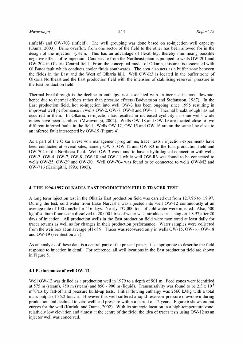
deep feed zone of OW-19, and finally 884 m to the deepest feed zone of OW-19. Other wells affected by injection into well OW-12 are OW-15, OW-16 and OW-18 (Figures 8-10). Current output and that during the test are tabulated below (Table 1). Their drilled depths are 1302, 1304 and 1407 m, respectively. Their lateral distances from well OW-12 are 218, 444 and 198 m, respectively. Apart from well OW-18, the remaining wells affected by injection into well OW-12 have experienced an increase in mass output accompanied by enthalpy drop. Well OW-16 is the most affected with a current flowing enthalpy of 1381 kJ/kg. Flowing enthalpies of wells OW-15 and OW-19 are over 1800 kJ/kg. Enthalpy drop observed in well OW-16 may indicate pressure recovery and less intensive reservoir boiling next to the well. This could also be associated with the same observation in wells OW-15 and OW-19, but to a lesser degree. This may suggest that the inferred fault close to well OW-19 could be recharging. OW-18 is close to the intersection of another fault and that intercepted by well OW-19. Since OW-18 appears to have poor recharge, then it is possible that the recharging fault intercepted by OW-19 dips in the direction of wells OW-15 and OW-16. The other inferred fault close to well OW-18 may be non-recharging.

TABLE 1: Output of wells in the East production field with tracer recovery

Steam (tons/hr) Water (tons/hr) Mass (tons/hr) Enthalpy (kJ/kg) Well no. 1996 2001 1996 2001 1996 2001 1996 2001

OW-15 OW-16 OW-18 OW-19

29.8 47.2 34.1 19.4

20.3 27.5 23.4 19.0

1.3 15.5 1.1 1.3

10.6 52.7 1.1

13.8

31.2 64.6 35.3 20.8

30.6 80.3 24.5 32.8

2651 2181 2675 2603

2034 1381 2663 1868


1980 1984 1988 1992 1996 2000 2004Time (year)

0

20

40

60

80

100

Mas

s, w

ater

and

ste

am o

utpu

t (to

ns/h

r)

0

1000

2000

Enth

alpy

(kJ/

kg)


Injectionperiod


1980 1984 1988 1992 1996 2000 2004Time (year)

0

100

200

300

Mas

s, w

ater

and

ste

am o

utpu

t (to

ns/h

r)

0

1000

2000

3000

Enth

alpy

(kJ/

kg)


Injection period


1980 1984 1988 1992 1996 2000 2004Time (year)

0

20

40

60

80

100

Mas

s, w

ater

and

ste

am o

utpu

t (to

ns/h

r)

0

1000

2000

3000

Enth

apy

(kJ/

kg)


Injection period

Report 12 Mwawongo

247

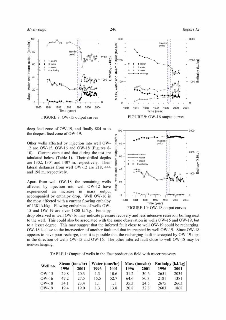
4.3 Tracer returns Figures 11-14 present tracer recovery curves in the East production field. Tracer breakthrough time ranged from 3 days in well OW-15, 46 days in well OW-16, 20 days in well OW-18, to 14 days in well OW-19. Well OW-15 recorded the highest tracer concentrations at an early time. OW-16 had the lowest tracer concentration. Tracer concentrations observed in wells OW-18 and OW-19 were comparable. Low concentrations in OW-16 could be due to a long flowpath connecting it to well OW-12. Tracer dilution as a result of its proximity to a recharge zone can also affect the data obtained from this well. Half width time of the pulses was about 97 days for wells OW-18 and OW-19 but the same could not be obtained for wells OW-15 and OW-16 due to either an incomplete sampling period or low concentrations. Increase in waterflow was experienced in all the wells with well OW-18 being most affected. Cycling behaviour of the wells is also well illustrated by the waterflow curves (Figure 15).

FIGURE 11: OW-15 tracer returns

0 100 200 300Time (day)

0

0.02

0.04

0.06

0.08

Con

cent

ratio

n (k

g/m

3)

field datacalculated


0 100 200 300Time (day)

0

0.02

0.04

0.06

0.08

Con

cent

ratio

n (k

g/m

3)field datacalculated


0 100 200 300Time (day)

0

0.02

0.04

0.06

0.08

Con

cent

ratio

n (k

g/m

3)



0 100 200 300Time (day)

0

0.02

0.04

0.06

0.08

Con

cent

ratio

n (k

g/m

3)


Mwawongo Report 12

248

Scatter in the data could be due to cyclic behaviour of the wells and even contamination of the samples as the same personnel mixed the initial 500 kg flourescein slug and did the sampling. Coarse modelling of the noisy data by a tracer inversion program (TRINV- see section 6.3) resulted in single pulse models for wells OW-15 and OW-16, two pulses for well OW-18 and three pulses for well OW-19. Based on the resulting tracer breakthrough and geology of the East production field, the flowpaths connecting the injector well and those affected were conceptualised as shown in Figure 16. Injected fluid flow to well OW-15 could be through direct fractures while that to wells OW-18 and OW-19 is possibly through the lower Olkaria trachyte which is deeper, hence, making the flowpath longer and more dispersive. As mentioned earlier, the Olkaria rhyolite provides feed zones for almost all the wells in the East production field. It is then possible that injected fluids into this layer can flow into most of the East production field wells in the long run (Figure 16). Apart from well OW-18, all the other affected wells are located to the south of well OW-12. This indicates that most of the injected fluid was flowing southwards (Figure 5). 4.4 Post processing of flourescein concentrations Flourescein is an organic dye used to trace flowpaths of injected fluids through geothermal reservoirs. Its advantages are low detection levels, easy to analyse and almost absent in natural hydrological systems (Axelsson, 2003). Thermal degradation of flourescein has been studied up to 300°C in hydrothermal autoclaves at various fluid compositions, pHs and oxygen concentrations. At temperatures below 210°C, flourescein is a suitable tracer for use in geothermal reservoirs (Adams and Davis, 1991). Its ability to decay at elevated temperatures is also advantageous in that it can be repeatedly used as an inexpensive and easy to analyse tracer in the same field for tests lasting a few months.

FIGURE 15: OW-15, 16, 18 and 19 waterflow

0 100 200 300Time (day)

0

40

80

120

160

200

Wei

r hei

ght (

mm

)

OW-15OW-16OW-18OW-19

FIGURE 16: Conceptualised fluid flowpaths

Report 12 Mwawongo

249

4.4.1 Thermal degradation Experimental results have shown that flourescein decays by less than 10% in one month at temperatures below 210°C (Adam and Davis, 1991). Flourescein at constant pH decays according to a first order rate law given by:

( ) kto eCtC −= (1)

where C(t) = Concentration of flourescein after heating (mg/l);

Co = Initial concentration (mg/l); t = Time (s); and k = A decay parameter (s-1).

Temperature dependent decay parameter k can be described by an Arrhenius relationship as (Rose et al., 2000):

)/( RTEaAek −= (2) where Ea = Energy of activation (J/mol);

A = Pre-exponential constant (s-1); T = Sample absolute temperature (K); and R = Universal gas constant = 8.31 J/mol K

During the experiments of Adams and Davis (1991), flourescein was subjected to temperatures ranging from 150 to 300°C. Half life of flourescein was found to be 150 days at 220°C and 37 days at 250°C. The activation energy Ea and the natural logarithm (ln) of the pre-exponential constant A were estimated as 143,300 (±6,620) J/mol and 18.25 (±1.44) s-1 respectively (Adam and Davis, 1991). 4.4.2 Thermal decay correction In the Olkaria East production field, downhole temperatures encountered in the reservoir are over 250°C as can be seen from the conceptual model of the field (Figure 3). This is higher than 210°C at which the decay of flourescein is negligible. Therefore, it is of interest to study the performance of flourescein at temperatures typical for the East production field. For the purpose of this analysis, values for the activation energy (Ea) and the pre-exponential constant A were selected from the experimental data above and used to correct the field data for thermal decay. The curve “best” matching the field data at the early time when decay was assumed negligible was taken to represent an effective flow channel temperature. Figures 17 and 18 below show tracer returns corrected for thermal decay at 150-175°C. The correction parameters used to correct the field data are tabulated below (Table 2). At 150°C, the tracer decay was negligible up to 120 days. After 144 days, the corrected tracer concentration obtained from well OW-18 started to rise. The same behaviour was observed in OW-19 after 167 days. Increase in

TABLE 2: Correction parameters for thermal decay

Experimental parameters Correction parameters used

k at 270°C k at 290°C k at 150°C k at 167°C k at 175°C 1.39 (±0.04) ×10-6 4.29 (±0.10) ×10-6 6×10-12 3×10-11 6×10-11

Ea ln A

143,300 (±6,620) J/mol18.25 (±1.44) s-1

149,920 J/mol16.81 s-1

149,920 J/mol 16.81 s-1

149,920 J/mol16.81 s-1

Mwawongo Report 12

250

tracer returns in this manner is most likely due to low tracer concentration at late times. These low concentrations are close to detection limits, meaning that the noise level of the data is high. By carrying out thermal correction, a small detection error can be amplified to an unrealistically high value. Due to this, the author decided to reject the late time data for possible thermal decay correction. Well OW-18 and OW-19 indicated good thermal decay correction up to a temperature of 167°C. This could be the effective temperature of the flow channels for these wells. Tracer returns obtained from OW-15 were not corrected due to incomplete sampling and the short breakthrough time observed in this well which was much less than the half life of flourescein. Data from OW-16 are hard to correct for thermal decay due to low tracer concentration obtained from the well. Injected fluids rich in oxygen result in rapid degradation of flourescein but the effect is highly diminished in alkaline fluids (Adams and Davis, 1991). Cold lake water is rich in dissolved oxygen but this was not considered in this analysis. It was assumed that its effect could be countered by the high pH in the Olkaria East reservoir. 5. MODELLING TRACER FLOW IN A FRACTURE 5.1 One-dimensional flow channel model Numerical modelling is one of the best methods available for detailed 2-D and 3-D analysis of flow of mass, tracer and heat as encountered in geothermal reservoirs. However, analytical solutions should first be adopted to solve specific aspects of tracer flow. Such solutions are available in literature, in particular simple 1-D flow channel models. These models approximately estimate some basic geometric properties of flowpaths that channel tracer from injection to a production well. Permeability in Olkaria is fracture controlled. A Simple 1-D model can therefore be used for coarse modelling of the flowpaths. In this analysis, a 1-D model was used to give an initial estimate of the fracture geometry and mass flowrate to be used in a later more detailed 2-D model.

FIGURE 17: Tracer returns for OW-18 corrected for thermal decay

0 100 200 300Time (day)

0

0.02

0.04

0.06

0.08

0.1

Con

cent

ratio

n (k

g/m

3)

field datacorrected 150°Ccorrected 167°Ccorrected 175°C

FIGURE 18: Tracer returns for OW-19 corrected for thermal decay

0 100 200 300Time (day)

0

0.02

0.04

0.06

0.08

0.1

Con

cent

ratio

n (k

g/m

3)

field datacorrected 150°Ccorrected 167°Ccorrected 175°C

Report 12 Mwawongo

251

5.2 Governing equations Tracer flow in a 1-D flow channel is governed by the following differential equation:

tC

xCu

xCD

∂∂

+∂∂

=∂∂

2

2

(3)

where C = Tracer concentration (kg/m3); and

D = Dispersion coefficient of the flow channel (m2/s). D is a sum of molecular and mechanical dispersion. The latter (mechanical dispersion) dominates and is often called αL (longitudinal dispersion) while the molecular dispersion is often neglected in tracer analysis. The mean fluid velocity u (m/s) is given by:

φρA

qu = (4)

where A = Cross-sectional area of the flow channel (m2);

q = Flowrate in the flow channel (kg/s); φ = Porosity; and ρ = Fluid density inside the flow channel (kg/m3).

Tracer mass is conserved in the flow channel by the equation:

qCcQ = (5) where Q = Production rate (kg/s); q = Injection rate (kg/s); C = Tracer concentration at injection point (kg/m3); and c = Concentration of the same at production well (kg/m3). A solution to the governing Equation 3 in terms of distance x from injection point and time t from tracer injection is:

Dt

utxDtQ

Mutxc4

)(exp),(2−−

=π

(6)

where M = Mass of tracer injected (kg). In Olkaria, fluid samples for tracer analysis were generally collected from weir boxes at atmospheric pressures. These weir box tracer concentrations have to be converted to tracer concentrations in the reservoir by the equation (Ofwona, 1996):

QwCC w

r×

= (7)

where Cr = Tracer concentration in the reservoir (kg/m3);

Cw = Weir box concentration (kg/m3); and w = Weir water flow (kg/s).

An important aspect in tracer data analysis is to estimate the total amount of tracer recovered. Cumulative tracer mass recovered is given by (Axelsson, 2003):

Mwawongo Report 12

252

dssQsCtm i

t

ii )()()(0

×= ∫ (8)

where mi(t) = Indicates the cumulative tracer mass recovered in production well number i (kg),

as a function of time (s); Ci = Tracer concentration history of the well (kg/m3); and Qi = Production rate of the well in question (m3/s).

5.3 Inverse tracer modelling by TRINV A tracer inversion program (TRINV) is available for solving the governing Equation 6 shown above (Arason et al., 1993). The TRINV program is simple and easy to use for training purposes. Input to the program are comprised of the estimated length of a flow channel between injection and production wells obtained from the conceptual reservoir model, well locations and the likely positions of the feed zones (Figure 16). The user needs to select a group of initial model parameters to be inverted for. In this study, the maximum concentration and the time it occurs, estimated half width time of the tracer pulse, production rate of the well, mass of tracer injected, injection flowrate and the reservoir fluid density are chosen. Different view points can be selected as an output from the TRINV program. For the purpose of later thermal models, the author decided to select the flow channel cross-section area and porosity product (Aφ), the longitudinal dispersivity (αL), the mean fluid velocity (u) and percentage of the tracer mass recovered (Mr%). These parameters were chosen as they provide important properties for heat transfer models of the flow channel (see Section 7). An initial guess of model parameters initiates the inversion process of the tracer data after which the program gives a “best” model of the injector – production dipole. A non-linear least-square algorithm is used for tracer data inversion. Assumptions made in the analysis are:

• The flow channel connecting the injector and producer well is of a constant cross-section area; • Flow is one-dimensional; • Production rate is constant; • Injection rate is constant; • Molecular diffusion is neglected; • No phase changes take place in the flow channel; • Mass of the tracer is conserved hence thermal degradation and chemical reaction with the

reservoir fluids and rocks have to be corrected for before modelling; • Production rate is higher than injection rate; • Fluid density inside the flow channel is constant; and • The reservoir fluid is pure water.

In hot geothermal fields like Olkaria, not all injected water is sampled at the weir box some is converted to steam and transmitted to the power station. Not all tracer injected can be recovered; some is adsorbed in the reservoir rock matrix or it undergoes thermal degradation. In the analysis of the tracer recovery curves described in Section 5, matrix permeability as well as high tracer dispersion is indicated by wide tracer pulses while fracture permeability is related to sharp and narrow pulses. In this analysis, the TRINV program was used to estimate initial parameters of the interconnecting flow channels and the tracer mass recovered. Data from the field was filtered to simulate one pulse model which is less affected by data noise. Noise amplification by thermal correction also identified data points that were unrealistic and hence

Report 12 Mwawongo

253

omitted for further analysis. After filtering, TRINV program was used to model the data and the results are as shown in Figures 19-22. Table 3 shows the flow channel parameters obtained while Table 4 shows the same after correcting the returns for thermal decay.

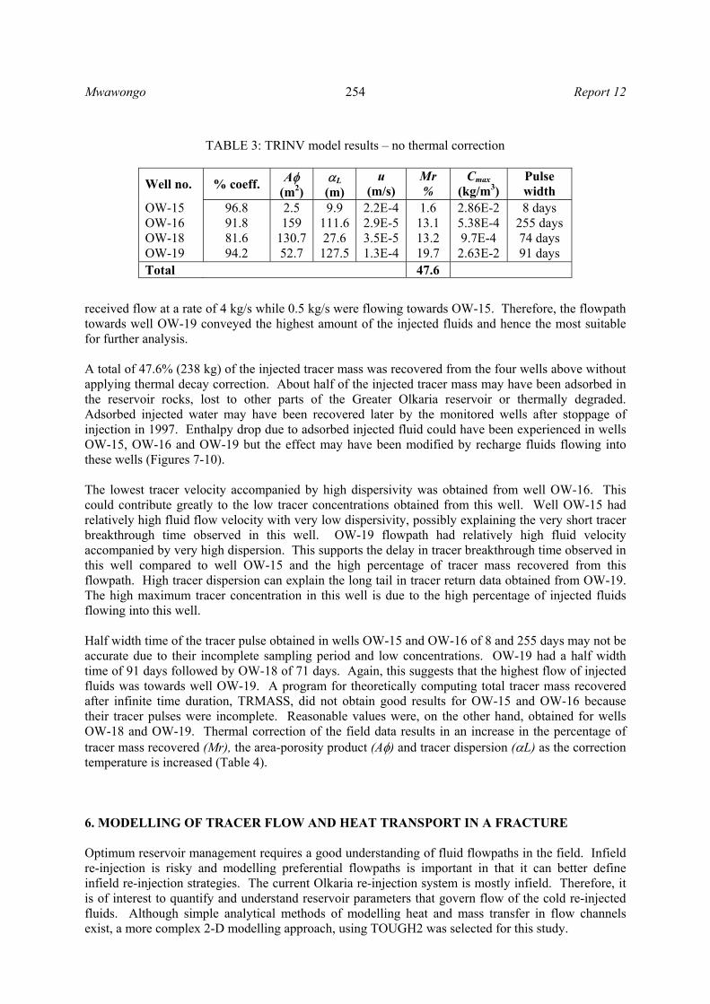
Tabulated results indicate that the lowest tracer mass recovery was from OW-15 which had the shortest breakthrough time while OW-19 had the highest tracer mass recovery of 19.7%. The low value of the tracer mass recovered from well OW-15 may not be accurate due to incomplete sampling from this well leading to an incomplete tracer pulse. Wells OW-16 and OW-18 had comparable percentage tracer mass recovered. Since the percentage tracer mass recovered is proportional to the flow of injected fluid in a particular flowpath, it then follows that out of the average 30 kg/s that were being injected during the test, 6 kg/s were flowing towards well OW-19. OW-16 and OW-18 each

FIGURE 19: Filtered tracer returns for OW-15 and simulated 1 pulse model

0 4 8 12 16 20Time (day)

0

0.01

0.02

0.03

0.04

Con

cent

ratio

n (k

g/m

3 )



0 100 200 300Time (day)

0

0.0002

0.0004

0.0006

0.0008

Con

cent

ratio

n (k

g/m

3)



0 100 200 300Time (day)

0

0.02

0.04

0.06

0.08

Con

cent

ratio

n (k

g/m

3)



0 100 200 300Time (day)

0

0.02

0.04

0.06

0.08

Con

cent

ratio

n (k

g/m

3)


Mwawongo Report 12

254

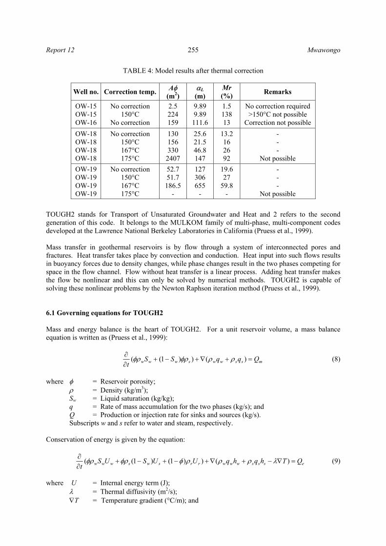
received flow at a rate of 4 kg/s while 0.5 kg/s were flowing towards OW-15. Therefore, the flowpath towards well OW-19 conveyed the highest amount of the injected fluids and hence the most suitable for further analysis. A total of 47.6% (238 kg) of the injected tracer mass was recovered from the four wells above without applying thermal decay correction. About half of the injected tracer mass may have been adsorbed in the reservoir rocks, lost to other parts of the Greater Olkaria reservoir or thermally degraded. Adsorbed injected water may have been recovered later by the monitored wells after stoppage of injection in 1997. Enthalpy drop due to adsorbed injected fluid could have been experienced in wells OW-15, OW-16 and OW-19 but the effect may have been modified by recharge fluids flowing into these wells (Figures 7-10). The lowest tracer velocity accompanied by high dispersivity was obtained from well OW-16. This could contribute greatly to the low tracer concentrations obtained from this well. Well OW-15 had relatively high fluid flow velocity with very low dispersivity, possibly explaining the very short tracer breakthrough time observed in this well. OW-19 flowpath had relatively high fluid velocity accompanied by very high dispersion. This supports the delay in tracer breakthrough time observed in this well compared to well OW-15 and the high percentage of tracer mass recovered from this flowpath. High tracer dispersion can explain the long tail in tracer return data obtained from OW-19. The high maximum tracer concentration in this well is due to the high percentage of injected fluids flowing into this well. Half width time of the tracer pulse obtained in wells OW-15 and OW-16 of 8 and 255 days may not be accurate due to their incomplete sampling period and low concentrations. OW-19 had a half width time of 91 days followed by OW-18 of 71 days. Again, this suggests that the highest flow of injected fluids was towards well OW-19. A program for theoretically computing total tracer mass recovered after infinite time duration, TRMASS, did not obtain good results for OW-15 and OW-16 because their tracer pulses were incomplete. Reasonable values were, on the other hand, obtained for wells OW-18 and OW-19. Thermal correction of the field data results in an increase in the percentage of tracer mass recovered (Mr), the area-porosity product (Aφ) and tracer dispersion (αL) as the correction temperature is increased (Table 4). 6. MODELLING OF TRACER FLOW AND HEAT TRANSPORT IN A FRACTURE Optimum reservoir management requires a good understanding of fluid flowpaths in the field. Infield re-injection is risky and modelling preferential flowpaths is important in that it can better define infield re-injection strategies. The current Olkaria re-injection system is mostly infield. Therefore, it is of interest to quantify and understand reservoir parameters that govern flow of the cold re-injected fluids. Although simple analytical methods of modelling heat and mass transfer in flow channels exist, a more complex 2-D modelling approach, using TOUGH2 was selected for this study.

TABLE 3: TRINV model results – no thermal correction

Well no. % coeff. Aφ (m2)

αL (m)

u (m/s)

Mr %

Cmax (kg/m3)

Pulse width

OW-15 OW-16 OW-18 OW-19

96.8 91.8 81.6 94.2

2.5 159

130.7 52.7

9.9 111.6 27.6

127.5

2.2E-4 2.9E-5 3.5E-5 1.3E-4

1.6 13.1 13.2 19.7

2.86E-2 5.38E-4 9.7E-4

2.63E-2

8 days 255 days 74 days 91 days

Total 47.6

Report 12 Mwawongo

255

TOUGH2 stands for Transport of Unsaturated Groundwater and Heat and 2 refers to the second generation of this code. It belongs to the MULKOM family of multi-phase, multi-component codes developed at the Lawrence National Berkeley Laboratories in California (Pruess et al., 1999). Mass transfer in geothermal reservoirs is by flow through a system of interconnected pores and fractures. Heat transfer takes place by convection and conduction. Heat input into such flows results in buoyancy forces due to density changes, while phase changes result in the two phases competing for space in the flow channel. Flow without heat transfer is a linear process. Adding heat transfer makes the flow be nonlinear and this can only be solved by numerical methods. TOUGH2 is capable of solving these nonlinear problems by the Newton Raphson iteration method (Pruess et al., 1999). 6.1 Governing equations for TOUGH2 Mass and energy balance is the heart of TOUGH2. For a unit reservoir volume, a mass balance equation is written as (Pruess et al., 1999):

msswwswww QqqSSt

=+∇+−+∂∂ )())1(( ρρφρφρ (8)

where φ = Reservoir porosity;

ρ = Density (kg/m3); Sw = Liquid saturation (kg/kg); q = Rate of mass accumulation for the two phases (kg/s); and Q = Production or injection rate for sinks and sources (kg/s).

Subscripts w and s refer to water and steam, respectively. Conservation of energy is given by the equation:

essswwwrrswswww QThqhqUUSUSt

=∇−+∇+−+−+∂∂ )())1()1(( λρρρφφρφρ (9)

where U = Internal energy term (J); λ = Thermal diffusivity (m2/s);

∇T = Temperature gradient (°C/m); and

TABLE 4: Model results after thermal correction

Well no. Correction temp. Aφ (m2)

αL (m)

Mr (%) Remarks

OW-15 OW-15 OW-16

No correction 150°C

No correction

2.5 224 159

9.89 9.89

111.6

1.5 138 13

No correction required >150°C not possible

Correction not possible OW-18 OW-18 OW-18 OW-18

No correction 150°C 167°C 175°C

130 156 330

2407

25.6 21.5 46.8 147

13.2 16 26 92

- - -

Not possible OW-19 OW-19 OW-19 OW-19

No correction 150°C 167°C 175°C

52.7 51.7 186.5

-

127 306 655

-

19.6 27

59.8 -

- - -

Not possible

Mwawongo Report 12

256

Qe = Rate of energy extraction (J/s). Subscripts w, s and r refer to water, steam and rock respectively. Momentum is conserved where two phases compete for pore space by introducing the Darcy equation with relative permeability for each phase. Darcy equations in two-phase flow are:

Liquid phase: ( )gPkkq ww

rww ρ

µ−∇−= (10)

Steam phase: ( )gPkkq ss

rss ρ

µ−∇−= (11)

where k = Absolute permeability (m2); krw = Relative permeability of the water phase;

krs = Relative permeability of the steam phase; ∇P = Pressure gradient (Pa/m); ρ = Density of the water or steam phase (kg/m3); as indicated by subscripts w and s,

respectively; and g = Acceleration due to gravity = 9.81 m/s2.

The term ρg is only applicable in vertical flow. Olkaria is a two-phase reservoir with Equations 10 and 11 being applicable everywhere. 6.2 Equation of state Fluid equation of state 1 (EOS1) is the most basic module of TOUGH2 used for solving mass and energy equations shown above. It assumes that the reservoir fluid is pure water/steam, without the presence of dissolved minerals or noncondensible gasses. The module neglects vapour pressure lowering due to capillary effects. Diffusion effects can be modelled with the option of two types of water, however, these were neglected in this analysis. EOS1 has a capability of representing two waters of identical physical properties which contain different trace elements by tracking their mass balances. With the two waters option, the primary variables are pressure, temperature and mass fraction of water two (Pruess et al., 1999). Where a chemical tracer to be tracked causes only negligible changes in the thermodynamic properties of water, the two waters option of TOUGH2 is suitable for numerical model development. The mass fraction of water two is proportional to the tracer to be tracked, hence, the two waters option can be used for modelling tracer returns in flowpaths. Tracer data can be used to calibrate the two waters model, after which the model can be used for predicting temperature distribution inside flow channels of various injection scenarios and geometry. Temperature recovery of the reservoir after stoppage of re-injection can also be predicted. 7. TRACER MODELLING 7.1 Wells 12 and 19 injection - production dipole Initial TRINV results indicate that well OW-19 recovered most of the tracer (19.7%) compared to the other affected wells (Tables 3 and 4). Now it is of interest to characterize the conduit that channelled the tracer from injection well 12 to production well 19. This is simply achieved by assuming that the flow channel is a vertical fracture that connects the two wells. By assuming 50% porosity for the flow

Report 12 Mwawongo

257

channel model, the fracture dimensions were found to be 800 m high × 400 m wide × 2 m thick. The 400 m was from the inter-well distance which is accurately known since the wells are both vertical while the 800 m elevation separation was known from feed zones depths. These fracture properties were used to model the tracer return curves using TOUGH2. In general, TOUGH2 models consist of a number of grid elements connected to each other. Each element is assigned appropriate rock type with different rock properties based on the conceptual model and geology of the reservoir. Initial grid blocks for this model were 50 m long, 50 m high and 2 m wide, covering the above mentioned horizontal distance of 400 m and a vertical distance of 800 m. Sample problem number 3 in the TOUGH2 user´s manual was adopted here for model development. This is a fracture model where its walls are modelled as semi-infinite half spaces of impermeable rock at 250°C, providing conductive heat transfer only. Mass transfer across the wall was not allowed for. For this type of analysis, TOUGH2 uses a semi-analytical treatment developed by Vinsome and Westerveld (1980) which requires no explicit representation of the conductive domains hence reducing the problem to a 2-D one (Pruess, 2002). For the model calibration, injection was done at the top and production was from the bottom to reproduce the conceptualised field reservoir scenario for wells OW-12 and OW-19 injection - production dipole. To make the input file suit the two waters option, the following changes had to be done to sample problem 3 of the TOUGH2 User’s manual:

• Block MULT was added and changed to 2, 3, 2, 6; • Every element was assigned a known non-zero fraction of water 2; • Tracer contaminated water is defined as water 2; • Water 2 in fluid sinks/sources in GENER block is defined as COMPONENT 2 while pure

water is COMPONENT 1.

The TOUGH2 code preserves mass of waters 1 and 2, and computes these two mass fractions for each model element at all times. In order to convert mass fraction of water 2 to tracer concentration, the following applies (Björnsson 1997), where tracer concentration C injected with water 2 is given by the equation:

oCXC ×= 2 (12) where X2 = Mass fraction of water two; and

Co = Initial concentration of the tracer slug that was injected into well OW-12 (kg/m3). Time steps for the iterations should be short enough to cover the tracer injection time which may last a few minutes to a few hours. This was achieved by introducing the block TIMES in the input file. 7.2 Modelling process The modelling process progressed by first making a MESH using the mesh maker inbuilt in TOUGH2. This resulted in a Cartesian 2-D mesh of 128 active elements. A dummy block of negative volume and confining bedrock type was added at the end of the ELEME block to provide thermal data for the conductive boundaries. Hydrostatic pressure equilibrium was then calculated for the fracture. Six kg/s of water one was injected for 20 days in accordance with the progress of the 1998 -1997 tracer test. At that point in time, injection of the tracer slug was introduced as water 2 pumped for one hour at a rate of 8 kg/s. After injection of water two, injection of water one was restarted and continued for the entire simulation time of 20 years. Results from the simulation runs were matched with the tracer return data obtained from the field to calibrate the model.

Mwawongo Report 12

258

7.3 Calibration and “best model” The fracture model of well dipole 12-19, is to be calibrated against the tracer recovery curve of well OW-19. The procedure was as follows. Some typical reservoir rock parameters were given an initial value and the model response to one year injection, including the tracer slug, monitored at the outlet point which is the productive feedzone of OW-19. It quickly turned out that the model is most sensitive to the fracture porosity. That should not be surprising, since the actual velocity of the tracer

slug is given by the Darcy flow velocity divided by the model porosity. Figure 23 shows several return curves obtained from the 2-D TOUGH2 vertical fracture model. The resulting model was subjected to several sensitivity studies. To ensure that tracer mass is conserved, the resulting mass fraction of water two was multiplied by the initial tracer concentration Co. The result is tracer concentration in water one. Integration of the product of the resulting tracer concentration in water one and its flowrate throughout the simulation period results in total mass of tracer injected as per Equation 8. Porosity of the model was varied from 8 to 15%. Lower porosities resulted in sharp and high tracer peaks of short half width time. Porosity had the highest effect on the model by greatly varying the fluid flow velocity, tracer breakthrough time and maximum tracer concentration. Changing the permeability had little effect on the tracer returns

in the short run. A good match of the tracer was not possible to attain with the initial porosity of 50%. This resulted in the half width time lasting through the entire simulation period. The model is, therefore, highly sensitive to pore volume. Reducing the thickness to 1 m resulted in a “best” match model (Table 5). The model is very sensitive to the initial concentration of the tracer. This varies the maximum tracer concentration obtained (peak height) as well as the half width time of the tracer pulse. Varying the injection time but conserving the initial tracer concentration varies the maximum concentration obtained (peak height) from a particular flowpath but not the half width time of the tracer pulse. From the match results, well OW-19 is connected to well OW-12 by a flowpath of 13% average porosity (Figure 23).

TABLE 5: Best model parameters for the wells OW12 – OW19 dipole

Model parameters Re-injection rate Fracture permeability Tracer injection rate (slug) Initial reservoir temperature Rock heat capacity Rock density OW-19 deliverability OW-19 bottom hole pressure OW-12 injection temperature Porosity Initial tracer concentration, Co

6 kg/s 200x10-15 m2 8 kg/s for 1 hour 250°C 1000 kJ/kg°C 2650 kg/m3 4x10-12 170 bars 20°C 15% 25 kg/m3

FIGURE 23: TOUGH2 tracer matching curves for OW-19

0 100 200 300

Time (day)

0

0.02

0.04

0.06

0.08

Con

cent

ratio

n (k

g/m

3)

field data8% porosity13% porosity15% porosity42 min. injection1 hr injection

Report 12 Mwawongo

259

8. LONG TERM THERMAL PERFORMANCE OF FRACTURE MODEL 8.1 Model results The “best” model calibrated by tracer returns (Table 5) was used for long term cooling predictions. This was achieved by changing the model fluid back to the one water model and using the EOS1 for modelling transfer of mass and heat in a vertical fracture. Now an optimal design of a re-injection system should result in maximum heating of the injected fluid and minimal cooling of the reservoir at production points. The author, therefore, decided to select outlet temperature of the 2-D fracture model as criteria for the thermal performance analysis. An injection rate of 8 kg/s was used to predict temperature distribution in the fracture for a period of 20 years at varied inlet temperatures, fracture dimensions, porosity and permeability. Figure 24 shows model performance for variable injectate temperatures. Obtained results indicate cooling of up to 55°C in twenty years while injecting at 20°C (Figure 24). Injecting at 150°C will cool the rocks by 25°C in the same period. Porosity variation has negligible effect on reservoir cooling (Figure 25). Cooling at a constant injection temperature and flowrate was shown to be affected by permeability of the fracture (Figure 26). At a constant injection temperature, an increase in permeability results in early onset of cooling and lower final outlet temperature at the end of simulation time (Figure 26).

After 20 years of injection, a resulting model temperature profile in the fracture zone at well OW-19 is shown in Figure 27. From the initial formation temperature, the heat mining process will progress with a downhole temperature drop of 90°C from the initial formation temperature of about 290°C. Outlet temperature of the injected fluids is expected to be 200°C after 20 years. The model indicates that cooling of the productive zone starts after 11/2 years when the temperature drops by 0.5°C. This suggests that cold water can be injected for one and a half years then stopped to allow the formation to recover and injected water adsorbed in the rock matrix to boil to steam. At the time of temperature recovery, the re-injection process can be shifted to another site far away from OW-19 (e.g. OW-6 or OW-14).

FIGURE 24: Simulated outlet temperature at OW-19 at varied injection temperature

0 4 8 12 16 20Time (year)

120

160

200

240

280

Tem

pera

ture

(°C

)

8 kg/s at 20°C8 kg/s at 100°C8 kg/s at 150°C

FIGURE 25: Simulated outlet temperature at OW-19 at varied fracture porosity

0 4 8 12 16 20Time (year)

120

160

200

240

280

Tem

pera

ture

(°C

)

13% porosity20% porosity30% porosity

Injection at 20°C

Mwawongo Report 12

260

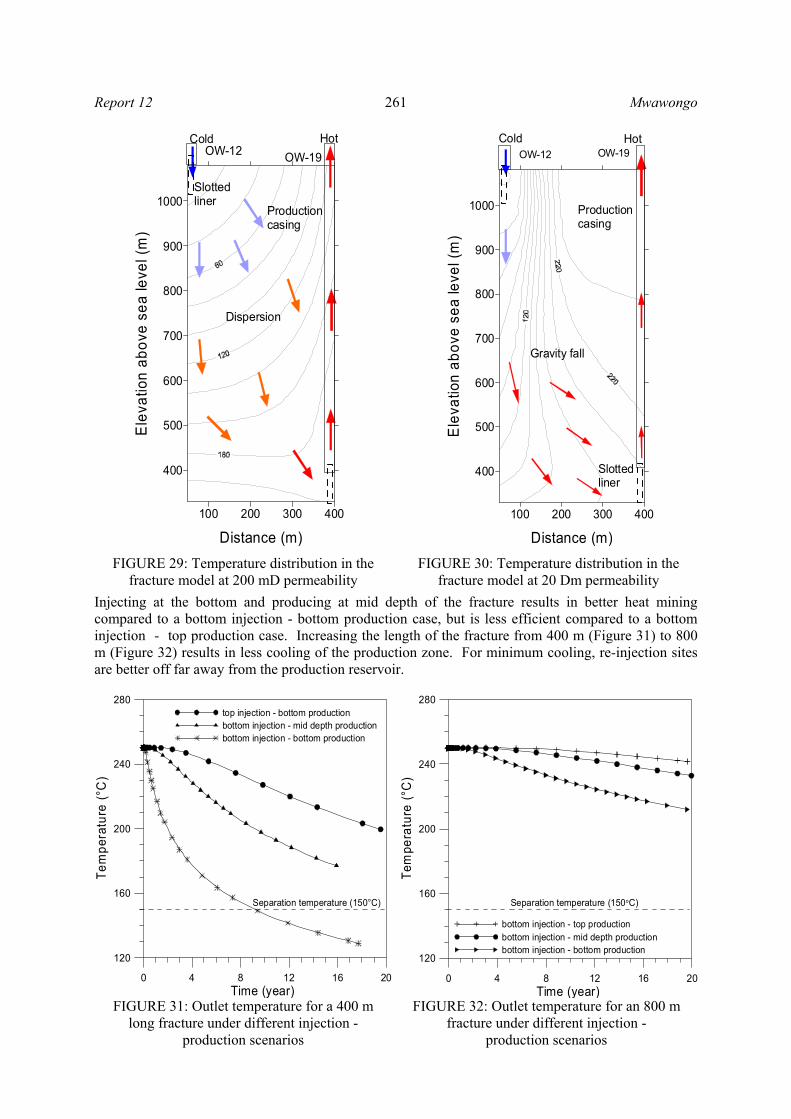
Shut-in downhole pressure profiles of the well indicate 40 bar-a at the top and about 100 bar-a at the bottom of the fracture zone. A pivot point occurs in the fracture zone at about 400 m a.s.l. indicating a reservoir pressure of 80 bar-a. Therefore, the main feed zone of the well occurs at this depth (Figure 28). Flashing occurs below the feed zone during flowing suggesting the existence of another feed zone below the fracture zone. Two-phase conditions occur in the fracture zone during flow. Pressure drawdown during flow at the fracture zone is 25 bar-a (Figure 28). From the initial formation temperature of 290°C and a flowing pressure of 60 bar-a, the two-phase conditions at the fracture will change to saturation conditions at 275°C. This allows for only 15°C cooling from the initial temperature, which according to the model will occur after 6 years. Gravity effects were less pronounced at a permeability of 200 mD (Figure 29) but the same were enhanced at a permeability of 20 Dm (Figure 30). Good vertical permeability results in water sinking deep into the reservoir, hence, reaching the hot reservoir rocks at the bottom. This interaction leads to an increase in heat mining efficiency from the reservoir rocks.

FIGURE 26: Simulated outlet temperature at OW-19 at varied fracture permeability

0 4 8 12 16 20Time (year)

120

160

200

240

280

Tem

pera

ture

(°C

)

k = 20 mDk = 200 mDk = 20 D

Separation temperature 150oC

100 200 30060 80 120 140 160 180 220 240 260 280 320 340

Temperature (°C)

0

1000

2000

Ele

vatio

n ab

ove

sea

leve

l (m

)

model profile28-1-8221-1-829-12-81

Initial model temperature

Fracturezone

Productioncasing

Slottedliner

Well OW-19

Cooledzone

Sep. temp. 150°C

FIGURE 27: Simulated and measured temperature profiles in and near well OW-19;

the simulated profile applies after 20 years of injection

0 40 80 120 160 200Pressure (bar-g)

0

1000

2000

Ele

vatio

n ab

ove

sea

leve

l (m

)

25-11-84 flowing27-1-82 shut-in4-1-82 shut-in9-11-81 shut-in

Pivotpoint

Flowing fracturepressure drop

Well OW-19Productioncasing

Slottedliner

Model downholepressure

Fracturezone

FIGURE 28: Downhole pressure profiles OW-19

Report 12 Mwawongo

261

Injecting at the bottom and producing at mid depth of the fracture results in better heat mining compared to a bottom injection - bottom production case, but is less efficient compared to a bottom injection - top production case. Increasing the length of the fracture from 400 m (Figure 31) to 800 m (Figure 32) results in less cooling of the production zone. For minimum cooling, re-injection sites are better off far away from the production reservoir.

FIGURE 31: Outlet temperature for a 400 m long fracture under different injection -

production scenarios

0 4 8 12 16 20Time (year)

120

160

200

240

280

Tem

pera

ture

(°C

)

top injection - bottom productionbottom injection - mid depth productionbottom injection - bottom production

Separation temperature (150°C)

FIGURE 32: Outlet temperature for an 800 m fracture under different injection -

production scenarios

0 4 8 12 16 20Time (year)

120

160

200

240

280

Tem

pera

ture

(°C

)

bottom injection - top productionbottom injection - mid depth productionbottom injection - bottom production

Separation temperature (150oC)

FIGURE 30: Temperature distribution in the fracture model at 20 Dm permeability

100 200 300 400

Distance (m)

400

500

600

700

800

900

1000

Ele

vatio

n ab

ove

sea

leve

l (m

)

OW-12 OW-19

Gravity fall

Production casing

Slotted liner

Cold Hot

100 200 300 400

Distance (m)

400

500

600

700

800

900

1000

Ele

vatio

n ab

ove

sea

leve

l (m

) OW-12 OW-19

Dispersion

Production casing

Slotted liner

Cold Hot

FIGURE 29: Temperature distribution in the fracture model at 200 mD permeability

Mwawongo Report 12

262

9. DISCUSSION Tracer analysis in two-phase flow is complicated by mobility effects due to phase changes. This makes numerical methods the most reliable way for analysing tracer returns from such fields. Well OW-19 and OW-18 had long tracer tails which indicate good tracer dispersion in the reservoir. This is supported by the wide width of the tracer pulses observed. Tracer flow in such paths is through the rock matrix rather than direct paths characterized by short and sharp tracer pulses. However, the low permeability used in the fracture model could still simulate a dispersive process. Re-injection can result in enthalpy decline in the field, reducing the pumping capability of wells. Low enthalpies will result in low wellhead pressures accompanied by a loss of high pressure steam especially for wells that flash in the well bore like OW-19. In such a case, re-injection process resulting in a rising of the flashing point in the well bore should be avoided. Gravity effects resulting from high vertical permeability enhances heat mining efficiency due to the sinking of the injected fluids deep into the reservoir. Sites with high vertical permeability may, therefore, be best for re-injection. This effect is well illustrated by the temperature section at 20 Dm permeability (Figure 30). OW-19 had the highest fraction of tracer recovered and has the deepest feedpoint compared to the other affected wells. This implies that gravity effects may have played a role in transporting the tracer towards well OW-19. Low permeability in the fracture tends to simulate a dispersive injection process. This means that more injected fluid is pushed into the rock matrix. Olkaria is generally associated with low fracture permeability. In such reservoirs the re-injection process can still be beneficial in the long term because the water adsorbed in the rock matrix can boil to steam as the pressure declines while the reservoir rocks are still hot. This is expected to occur during the temperature recovery period when the re-injection process is shifted to another site. OW-15 had the shortest tracer breakthrough time hence the shortest and the most direct path to OW-12. This is a critical well to monitor during re-injection into well OW-12. However, the well still has high flowing enthalpy (> 2000 kJ/kg). Therefore, injected fluid flow into this well can still result in increased steam flow. The ultimate goal of infield re-injection is to recharge the liquid zone with water while maintaining the boiling level at the same depth. Total collapsing of the steam zone can be disastrous. Therefore, well OW-12 alone cannot manage this process. With additional re-injection into well OW-3 and intermittent re-injection into wells OW-6, OW-12 and OW-14, the re-injection process will be more dispersive. This may achieve the ultimate goal. It is, therefore, proposed that tracer tests be conducted in well OW-14 and OW-6 (Figure 5). The fracture model used for cooling predictions was quite pessimistic in that it assumed 13% porosity, rather than the 6% used in the recent model studies for Olkaria (Ofwona, 2002). The model temperature used, 250°C, is much lower than that observed in the heat-up runs for the same well, 290°C in the fracture zone. The most efficient heat mining process is one which will result in the least cooling of the production zone at a constant low injection temperature. Injecting at the bottom and producing at the top results in the least cooling of the production zone. Therefore, deep re-injection is preferred to shallow re-injection. Injecting at the bottom and producing at the same level results in the highest cooling, hence simulating a short circuit effect. In a liquid-dominated zone, this effect may result in a dense liquid phase falling into deeper levels leaving a steam cap at the top. The result will be a heat pipe effect mining the reservoir heat and conducting it to the cap rock, leading to heat loss due to enhanced surface

Report 12 Mwawongo

263

manifestations like steam vents and hot springs. The same effect is observed from medium depth production, but to a lesser degree. Doubling the lateral distance from 400 to 800 m led to a better heat mining effect. This implies that re-injection sites are better placed far away from the production reservoir. However, limited infield reinjection may be unavoidable for a relatively low-permeability field like Olkaria. For the OW-12 and OW-19 injection–production dipole analysed, top injection with bottom production results in cooling rates close to the best heat mining scenario. Re-injection into well OW-12 can, therefore, be done with careful monitoring of the interconnected production wells. Hot re-injection at separation pressure is most preferable. The best method may be intermittent cold injection. Hence the process may not cool OW-19 by much. However, the interconnecting paths with the other wells need to be analysed in the same manner for re-injection effects. Silica scaling has been associated with permeability loss of injection wells. This is mainly due to thermal fronts generated in the reservoir by injecting low-temperature fluids, leading to over-saturation with respect to silica in the reservoir fluids. From the thermal predictions above, this may not be a problem in the production well because outlet temperature is above 150°C. But it will be a problem in the injection well. This makes hot re-injection at 150°C better than cold. Wells OW-26, OW-29 and OW-30 are a possible source of hot brine for this process as they are all at a higher elevation than well OW-12. Despite well OW-12 having declined to zero pressure during production, the tracer test results indicate that the well still has good injectivity. Tracer breakthrough observed in the other production wells makes well OW-12 a suitable candidate for infield re-injection with careful monitoring due to its location, almost in the centre of the field. 10. CONCLUSIONS From the analysis carried out and preceding discussions, the following can be concluded:

• The inferred fault close to OW-19 is a recharging fault and inclined in the direction of wells OW-15 and OW-16.

• OW-12 has good injectivity and can be used for infield re-injection with careful monitoring of

the other production wells in the field, in particular OW-15. Direct flowpaths connect OW-15 to well OW-12 while those to OW-18 and OW-19 are long and dispersive. Due to the relatively high elevation of wells OW-26, OW-29 and OW-30, separated brines from these wells can easily flow into well OW-12 (infield) by gravity.

• During injection at fixed geometrical conditions, permeability has the highest impact on

cooling while porosity affects flow velocity. Re-injection sites should be in sites with high vertical permeability.

• In the Olkaria East production field, infield re-injection appears a feasible method of mining

heat at the centre of the field. Hot re-injection at 8 kg/s or less is preferred to cold. Re-injecting deep and producing from shallow zones is the best heat mining strategy.

• In the long term, it appears that re-injecting into the Olkaria Central field could be the most

appropriate site. It is possible that re-injecting into this sector and the resulting pressure

Mwawongo Report 12

264

increase can push re-injected fluids back to the East and Northeast fields with adequate residence time in the reservoir for heat mining.

• Flourescein is a suitable tracer for use in Olkaria East production field, especially for a short

term test lasting a few months. Its ability to decay makes it reusable in the same field with results from earlier tests not affecting later ones.

• Southward flow of the tracer further confirms the north to south flow of reservoir fluids

conceptualized in Olkaria.

ACKNOWLEDGEMENTS

I feel honoured to be a student of my supervisors Arnar Hjartarson, Grímur Björnsson and Gudni Axelsson. I would like to sincerely thank them for their assistance and guidance throughout my analysis and compilation of this report. My sincere gratitude to the UNU - GTP and the Government of Iceland for awarding me this scholarship to participate in this wonderful programme. Special thanks to the UNU staff Dr. Ingvar B. Fridleifsson, Mr. Lúdvík S. Georgsson and Mrs. Gudrún Bjarnadóttir for their generous help, care and good advice during my entire study period. I also thank all members of ISOR and Orkustofnun who participated in this programme to make it such a big success. Input from other organisations in Iceland is also highly appreciated. I am grateful to my employer Kenya Electricity Generating Company Ltd (KenGen) for providing data used in this study and granting me a sabbatical leave to be part of the UNU-GTP of 2004. To the other UNU fellows I say, thank you very much for your wonderful company that made me feel at home away from home. To my beloved wife Verity and son Lenny, words are not enough to express my sincere thanks to you for your sacrifice, love and prayers throughout my entire stay in Iceland – may God bless you.

REFERENCES Adams, M.C., and Davis J., 1991: Kinetics of flourescein decay and its application as a geothermal tracer. Geothermics, 20, 53-66. Arason, Th., Björnsson, G., Axelsson, G., Bjarnason, J.Ö., and Helgason, P., 2004: ICEBOX – geothermal reservoir engineering software for Windows. A user’s manual. ISOR, Reykjavík, report 2004/014, 80 pp. Axelsson, G., 2003: Tracer tests in geothermal resource management: analysing and cooling predictions. ISOR, Reykjavík, unpublished report. Axelsson, G., 2004: Re-injection and geothermal resource management. UNU-GTP, Iceland, unpublished lecture notes. Björnsson, G., 1997: Reservoir modelling integrating isotope and chemical data. International Atomic Energy Agency, Project ELS/8/005-03, report on an expert mission to El Salvador, 21 pp. Bödvarsson, G.S., and Pruess, K., 1984: History match and performance predictions for the Olkaria geothermal field. Kenya Power Company Ltd., internal report. Bödvarsson, G.S., and Pruess, K., 1987: Numerical simulation studies of the Olkaria geothermal field. Kenya Power Company Ltd., internal report.

Report 12 Mwawongo

265

Bödvarsson, G.S., and Stefánsson, V., 1987: Re-injection into geothermal reservoirs. Lawrence Berkeley Laboratory, University of California, Earth Sciences Division, 7 pp. Karingithi, C.W., 1993: Results of injection and tracer tests in Olkaria East production field. Kenya Power Company Ltd., internal report, 21 pp. Karingithi, C.W., 1995: Results of injection and tracer tests in Olkaria Northeast field in Kenya. Geoth. Res. Council, Trans., 19, 497-501. Kariuki, M., and Opondo, K., 2000: Status report on steam production and reservoir assessment of Olkaria East Field, 2nd half of 2000. Kenya Electricity Generating Company Ltd, internal report, 30 pp. Kariuki, M., and Ouma, P., 2002: Twenty years of exploitation of Olkaria East Field, Geoth. Res. Council, Trans., 26, 565-571. KPC, 1994: Brief of geothermal energy development at Olkaria Kenya. Status as in March. Kenya Power Company Ltd., internal report, 26 pp. Merz & McLellan-Virkir, 1981: Recommendations for further geothermal exploration at Olkaria. Kenya Power Company Ltd., internal report. Merz & McLellan-Virkir, 1986: Status report on steam production. The Kenya Power Company Ltd., Olkaria Geothermal Project, internal report. Mwawongo, G.M., 2002: Effects of re-injection/injection into well OW-03. Proceedings of the 2nd Kenya Electricity Generating Company Ltd. Technical Seminar, Nairobi, 152-159. Naylor, W.I., 1972: Geology of the Eburru and Olkaria prospects. U.N. Geothermal Exploration Project, report. Ofwona, C.O., 1996: Analysis of injection and tracer tests data from the Olkaria East geothermal field Kenya. Report 10 in: Geothermal Training in Iceland 1996. UNU-GTP, Iceland, 197-218. Ofwona, C.O., 2002: A reservoir study of the Olkaria East geothermal system, Kenya. University of Iceland, MSc thesis, UNU-GTP, Iceland, report 1, 74 pp. Ouma, P.A., 2003: Re-injection strategy in the Olkaria Northeast geothermal field, Kenya. Proceedings of the 2nd Kenya Electricity Generating Company Ltd. Geothermal Conference, Nairobi, 106-112. Pruess, K., 2002: Mathematical modeling of fluid and heat transfer in geothermal systems. UNU- GTP, Iceland, report 3, 92 pp. Pruess, K., Oldenburg, C., and Moridis, G., 1999: TOUGH2, user’s guide version 2.0. Lawrence Berkeley National Laboratory, 197 pp. Rose, P., Benoir, D., Lee, S.G., Tandia, B., and Kilbourn, P., 2000: Testing the naphthalene sulfonates as geothermal tracers at Dixie Valley, Ohaki and Awibengkok. Proceedings of the 25th Workshop on Geothermal Reservoir Engineering, Stanford University, Stanford, Ca., 7 pp.

Mwawongo Report 12

266

Shook, G.M., and Renner, J.L., 2002: An inverse model for Tetrad: Preliminary results. Geoth. Resourc. Council, Trans., 26, 119-122. Stefánsson, V., 1997: Geothermal reinjection experience. Geothermics, 26, 99-139. Vinsome, P.K.W., and Westerveld, J., 1980: A simple method for predicting cap and base rock heat losses in thermal reservoir simulators. J. Canadian Pet. Tech., 19-3, 87-90.

infield re-injection strategies in olkaria, kenya… · geothermal training programme reports 2004...

Documents