inferential statistics - unibo. · pdf filethe quantity of liquid inserted in a bottle has...
TRANSCRIPT

Inferential Statistics
POPULATION
SAMPLE
Statistical inference is the branch of statistics concerned with
drawing conclusions and/or making decisions concerning a pop-
ulation based only on sample data.
187
Statistical inference: example 1
• A clothing store chain regularly buys from a supplier large
quantities of a certain piece of clothing. Each item can be
classified either as good quality or top quality. The agree-
ments require that the delivered goods comply with standards
predetermined quality. In particular, the proportion of good
quality items must not exceed 25% of the total.
• From a consignment 40 items are extracted and 29 of these
are of top quality whereas the remaining 11 are of good
quality.
INFERENTIAL PROBLEMS:
1. provide an estimate of π and quantify the uncertainty asso-
ciated with such estimate;
2. provide an interval of “reasonable” values for π;
3. decide whether the delivered goods should be returned to the
supplier.
188
Statistical inference: example 1
Formalization of the problem:
• POPULATION:
all the pieces of clothes of the consignment;
• VARIABLE OF INTEREST:
good/top quality of the good (binary variable);
• PARAMETER OF INTEREST:
proportion of good quality items π;
• SAMPLE:
40 items extracted from the consignment.
The value of the parameter π is unknown, but it affects the
sampling values. Sampling evidence provides information on the
parameter value.
189
Statistical inference: example 2
• A machine in an industrial plant of a bottling company fills
one-liter bottles. When the machine is operating normally
the quantity of liquid inserted in a bottle has mean µ = 1
liter and standard deviation σ =0.01 liters.
• Every working day 10 bottles are checked and, today, the
average amount of liquid in the bottles is x = 1.0065 with
s = 0.0095.
INFERENTIAL PROBLEMS:
1. provide an estimate of µ and quantify the uncertainty asso-
ciated with such estimate;
2. provide an interval of “reasonable” values for µ;
3. decide whether the machine should be stopped and revised.
190

Statistical inference: example 2
Formalization of the problem:
• POPULATION:
“all” the bottles filled by the machine;
• VARIABLE OF INTEREST:
amount of liquid in the bottles (continuous variable);
• PARAMETERS OF INTEREST:
mean µ and standard deviation σ of the amount of liquid in
the bottles;
• SAMPLE:
10 bottles.
The values of the parameters µ and σ are unknown, but they
affect the sampling values. Sampling evidence provides informa-
tion on the parameter values.
191
The sample
• Census survey: attempt to gather information from each and
every unit of the population of interest;
• sample survey: gathers information from only a subset of the
units of the population of interest.
Why using a sample?
1. Less time consuming than a census;
2. less costly to administer than a census;
3. measuring the variable of interest may involve the destruc-
tion of the population unit;
4. a population may be infinite.
192
Probability sampling
A probability sampling scheme is one in which every unit in the
population has a chance (greater than zero) of being selected in
the sample, and this probability can be accurately determined.
SIMPLE RANDOM SAMPLING: every unit has an equal prob-
ability of being selected and the selection of a unit does not
change the probability of selecting any other unit. For instance:
• extraction with replacement;
• extraction without replacement.
For large populations (compared to the sample size) the differ-
ence between these two sampling techniques is negligible. In the
following we will always assume that samples are extracted with
replacement from the population of interest.
193
Probabilistic description of a population
• Units of the population;
• variable X measured on the population units;
• sometimes the distribution of X is known, for instance
(i) X ∼ N(µ, σ2);
(ii) X ∼Bernoulli(π).
194

Probabilistic description of a sample
• The observed sampling values are
x1, x2, . . . , xn;
• BEFORE the sample is observed the sampling values are
unknown and the sample can be written as a sequence of
random variables
X1, X2, . . . , Xn
• for simple random samples (with replacement):
1. X1, X2, . . . , Xn are i.i.d.;
2. the distribution of Xi is the same as that of X
for every i = 1, . . . , n.195
Sampling distribution of a statistic (1)
• Suppose that the sample is used to compute a given statistic,
for instance
(i) the sample mean X;
(ii) the sample variance S2;
(iii) the proportion P of units with a given feature;
• generically, we consider an arbitrary statistic
T = g(X1, . . . , Xn)
where g(·) is a given function.
196
Sampling distribution of a statistic (2)
• Once the sample is observed, the observed value of the statis-
tic is given by
t = g(x1, . . . , xn);
• suppose that we draw all possible samples of size n from the
given population and that we compute the statistic T for
each sample;
• the sampling distribution of T is the distribution of the pop-
ulation of the values t of all possible samples.
197
Normal population
• Suppose that X ∼ N(µ, σ2)
• in this case the statistics of interest are:
(i) the sample mean X =1
n
n∑
i=1
Xi
(ii) the sample variance S2 =1
n− 1
n∑
i=1
(Xi − X)2
• the corresponding observed values are
x =1
n
n∑
i=1
xi and s2 =1
n− 1
n∑
i=1
(xi − x)2,
respectively.
198

The sample mean
The sample mean is a linear combination of the variables forming
the sample and this property can be exploited in the computation
of
• the expected value of X, that is E(X);
• the variance of X, that is Var(X
);
• the probability distribution of X.
199
Expected value of the sample mean
For a simple random sample X1, . . . , Xn, the expected value of
X is
E(X) = E
(X1 +X2 + · · ·+Xn
n
)
=1
nE (X1 +X2 + · · ·+Xn)
=1
n[E(X1) + E(X2) + · · ·+E(Xn)]
=1
n(n× µ)
= µ
200
Variance of the sample mean
For a simple random sample X1, . . . , Xn, the variance of X is
Var(X
)= Var
(X1 +X2 + · · ·+Xn
n
)
=1
n2Var(X1 +X2 + · · ·+Xn)
=1
n2[Var(X1) + Var(X2) + · · ·+Var(Xn)]
=1
n2(n× σ2)
=σ2
n
201
Sampling distribution of the mean
For a simple random sample X1, X2, . . . , Xn, the sample mean X
has
• expected value µ and variance σ2/n;
• if the distribution of X is normal, then
X ∼ N
(µ,
σ2
n
)
• more generally, the central limit theorem can be applied to
state that the distribution of X is APPROXIMATIVELY nor-
mal.
202

The sample variance
• The sample variance is defined as
S2 =1
n− 1
n∑
i=1
(Xi − X)2
• if Xi ∼ N(µ, σ2) then
(n− 1)S2
σ2∼ χ2
n−1
• X and S2 are independent.
203
The chi-squared distribution
• Let Z1, . . . , Zr be i.i.d. random variables with distribution
N(0; 1);
• the random variable
X = Z21 + · · ·+ Z2
r
is said to follow a CHI-SQUARED distribution with r degrees
of freedom (d.f.);
• we write X ∼ χ2r ;
• E(X) = r and Var(X) = 2r.
204
Counting problems
• The variable X is binary, i.e. it takes only two possible val-
ues; for instance “success” and “failure”;
• the random variable X takes values “1” (success) and “0”
(failure);
• the parameter of interest is π, the proportion of units in the
population with value “1”;
• Formally, X ∼ Bernoulli(π) so that
E(X) = π and Var(X) = π(1− π).
205
The sample proportion (1)
• Simple random sample X1, . . . , Xn;
• the variable X takes two values: 0 and 1, and the sample
proportion is a special case of sample mean
P =
∑ni=1Xi
n
• the observed value of P is p.
206

The sample proportion (2)
• The sample proportion is such that
E(P) = π and Var(P) =π(1− π)
n
• for the central limit theorem, the distribution of X is approx-
imatively normal;
• sometimes the following empirical rules are used to decide if
the normal approximation is satisfying:
1. n× π > 5 and n× (1− π) > 5.
2. np(1− p) > 9.
207
Estimation
• Parameters are specific numerical characteristics of a popu-
lation, for instance:
– a proportion π;
– a mean µ;
– a variance σ2.
• When the value of a parameter is unknown it can be esti-
mated on the basis of a random sample.
208
Point estimation
A point estimate is an estimate that consists of a single value
or point, for instance one can estimate
• a mean µ with the sample mean x;
• a proportion π with a sample proportion p;
a point estimate is always provided with its standard error that
is a measure of the uncertainty associated with the estimation
process.
209
Estimator vs estimate
• An estimator of a population parameter is
– a random variable that depends on sample information,
– whose value provides an approximation to this unknown
parameter.
• A specific value of that random variable is called an estimate.
210

Estimation and uncertainty
• Parameter θ;
• the sampling statistics T = g(X1, . . . , Xn) on which estima-
tion is based is called the estimator of θ and we write
θ = T
• the observed value of the estimator, t, is called an estimate
of θ and we write θ = t;
• it is fundamental to assess the uncertainty of θ;
• a measure of uncertainty is the standard deviation of the
estimator, that is SD(T) = SD(θ). This quantity is called
the
STANDARD ERROR of θ and denoted by SE(θ).
211
Point estimation of a mean (σ2 known)
• Consider the case where X1, . . . , Xn is a simple random sam-
ple from X ∼ N(µ, σ2);
• Parameters:
– µ, unknown;
– assume that the value of σ2 is known.
• the sample mean can be used as estimator of µ: µ = X;
• the distribution of the estimator is normal with
E(µ) = µ and Var(µ) =σ2
n
• STANDARD ERROR µ
SE(µ) =σ√n
212
Point estimation of a mean with σ2 known: example
In the “bottling company” example, assume that the quantity
of liquid in the bottles is normally distributed. Then a point
estimate of µ is
• µ = 1.0065
• and the standard error of this estimate is
SE(µ) =σ√10
=0.01√10
= 0.0032
213
Point estimation of a mean (σ2 unknown)
• Typically the value of σ2 is not known;
• in this case we estimate it as σ2 = s2;
• this can be used, for instance, to estimate the standard error
of µ
SE(µ) =σ√n.
• In the “bottling company” example, if σ is unknown it can
be estimated as
SE(µ) =0.0095√
10= 0.0030
214

Point estimation for the mean of a non-normal population
• X1, . . . , Xn i.i.d. with E(Xi) = µ and Var(Xi) = σ2;
• the distribution of Xi is not normal;
• for the central limit theorem the distribution of X is approx-
imatively normal.
215
Point estimation of a proportion
• Parameter: π;
• the sample proportion P is used as an estimator of π
π = P
• this estimator is approximately normally distributed with
E(π) = π and Var(π) =π(1− π)
n
• the STANDARD ERROR of the estimator is
SE(π) =
√π(1− π)
n
and in this case the value of standard error is never known.
216
Estimation of a proportion: example
For the “clothing store chain” example the estimate of the pro-
portion π of good quality items is
• π =11
40= 0.275
• and an ESTIMATE of the standard error is
SE(π) =
√0.275(1− 0.275)
40= 0.07
217
Properties of estimators: unbiasedness
A point estimator θ is said to be an unbiased estimator of the
parameter θ if the expected value, or mean, of the sampling
distribution of θ is θ, formally if
E(θ) = θ
Interpretation of unbiasedness: if the sampling process was re-
peated, independently, an infinite number of times, obtaining in
this way an infinite number of estimates of θ, the arithmetic
mean of such estimates would be equal to θ. However, unbi-
asedness does not guarantees that the estimate based on one
single sample coincides with the value of θ.
218

Point estimator of the variance
The sample variance S2 is an unbiased estimator of the variance
σ2 of a normally distributed random variable
E(S2) = σ2.
On the other hand S2 is a biased estimator of σ2
E(S2) =(n− 1)
nσ2.
219
Bias of an estimator
Let θ be an estimator of θ. The bias of θ, Bias(θ), is defined as
the difference between the expected value of θ and θ
Bias(θ) = E(θ)− θ
The bias of an unbiased estimator is 0.
220
Properties of estimators: Mean Squared Error (MSE)
For an estimator θ of θ the (unknown) estimation “error” is given
by
|θ − θ|
The Mean Squared Error (MSE) is the expected value of the
square of the “error”
MSE(θ) = E[(θ − θ)2]
= Var(θ)+ [θ −E(θ)]2
= Var(θ)+Bias(θ)2
Hence, for an unbiased estimator, the MSE is equal to the vari-
ance.
221
Most Efficient Estimator
• Let θ1 and θ2 be two estimator of θ, then the MSE can be
use to compare the two estimators;
• if both θ1 and θ2 are unbiased then θ1 is said to be more
efficient than θ2 if
Var(θ1
)< Var
(θ2
)
• note that if θ1 is more efficient than θ2 then also MSE(θ1) <
MSE(θ2) and SE(θ1) < SE(θ2);
• the most efficient estimator or the minimum variance unbi-
ased estimator of θ is the unbiased estimator with the small-
est variance.
222
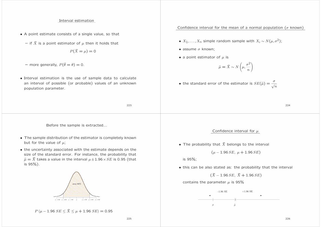
Interval estimation
• A point estimate consists of a single value, so that
– if X is a point estimator of µ then it holds that
P(X = µ) = 0
– more generally, P(θ = θ) = 0.
• Interval estimation is the use of sample data to calculate
an interval of possible (or probable) values of an unknown
population parameter.
223
Confidence interval for the mean of a normal population (σ known)
• X1, . . . , Xn simple random sample with Xi ∼ N(µ, σ2);
• assume σ known;
• a point estimator of µ is
µ = X ∼ N
(µ,
σ2
n
)
• the standard error of the estimator is SE(µ) =σ√n
224
Before the sample is extracted...
• The sample distribution of the estimator is completely known
but for the value of µ;
• the uncertainty associated with the estimate depends on the
size of the standard error. For instance, the probability that
µ = X takes a value in the interval µ±1.96×SE is 0.95 (that
is 95%).
µµ − 1 SEµ − 2 SEµ − 3 SE µ + 1 SE µ + 2 SE µ + 3 SE
area 95%
P(µ− 1.96 SE ≤ X ≤ µ+1.96 SE
)= 0.95
225
Confidence interval for µ
• The probability that X belongs to the interval
(µ− 1.96SE, µ+1.96SE)
is 95%;
• this can be also stated as: the probability that the interval
(X − 1.96SE, X +1.96SE)
contains the parameter µ is 95%
✛ ✲
-1.96 SE +1.96 SE
µ µ
226

Formal derivation of the 95% confidence interval for µ (σ known)
It holds that
X − µ
SE∼ N (0,1) where SE =
σ√n
so that
0.95 = P
(−1.96 ≤ X − µ
SE≤ 1.96
)
= P(−1.96 SE ≤ X − µ ≤ 1.96 SE
)
= P(−X − 1.96 SE ≤ −µ ≤ −X +1.96 SE
)
= P(X − 1.96 SE ≤ µ ≤ X +1.96 SE
)
227
Confidence interval for µ with σ known: example
In the bottling company example, if one assumes σ = 0.01
known, a 95% confidence interval for µ is
(1.0065− 1.96
0.01√10
; 1.0065 + 1.960.01√10
)
that is
(1.0065− 0.0062; 1.0065 + 0.0062)
so that
(1.0003; 1.0126)
228
After the sample is extracted...
On the basis of the sample values the observed value of µ = x
is computed. x may belong to the interval µ± 1.96× SE or not.
For instance
µµ − 1 SEµ − 2 SEµ − 3 SE µ + 1 SE µ + 2 SE µ + 3 SE
area 95%x
and in this case x belongs to the interval µ± 1.96× SE and, as
a consequence, also the interval (x − 1.96× SE; x+ 1.96× SE)
will contain µ.
229
a different sample...
A different sample may lead to a sample mean x that, as in the
example below, does not belong to the interval µ±1.96×SE and,
as a consequence, also the interval (x−1.96×SE; x+1.96×SE)
will not contain µ.
µµ − 1 SEµ − 2 SEµ − 3 SE µ + 1 SE µ + 2 SE µ + 3 SE
area 95% x
The interval (x−1.96×SE; x+1.96×SE) will contain µ for the
95% of all possible samples.
230

Interpretation of confidence intervals
Probability is associated with the procedure that leads to the
derivation of a confidence interval, not with the interval itself.
A specific interval either will contain or will not contain the true
parameter, and no probability involved in a specific interval.
Confidence intervals
for five different sam-
ples of size n = 25,
extracted from a nor-
mal population with
µ = 368 and σ = 15.
231
Confidence interval: definition
A confidence interval for a parameter is an interval constructed
using a procedure that will contain the parameter a specified
proportion of the times, typically 95% of the times.
A confidence interval estimate is made up of two quantities:
interval: set of scores that represent the estimate for the pa-
rameter;
confidence level: percentage of the intervals that will include
the unknown population parameter.
232
A wider confidence interval for µ
• Since it also holds that
P(µ− 2.58 SE ≤ X ≤ µ+2.58 SE
)= 0.99
µµ − 1 SEµ − 2 SEµ − 3 SE µ + 1 SE µ + 2 SE µ + 3 SE
area 99%x
µµ − 1 SEµ − 2 SEµ − 3 SE µ + 1 SE µ + 2 SE µ + 3 SE
area 99%x
• then the probability that (X−2.58SE, X+2.58SE) contains
µ is 99%.
233
Confidence level
The confidence level is the percentage associated with the in-
terval. A larger value of the confidence level will typically lead
to an increase of the interval width. The most commonly used
confidence levels are
• 68% associated with the interval X ± 1SE;
• 95% associated with the interval X ± 1.96SE;
• 99% associated with the interval X ± 2.58SE.
Where the values 1, 1.96 and 2.58 are derived from the standard
normal distribution tables.
234

Notation: standard normal distribution tables
• Z ∼ N(0,1);
• α value between zero and one;
• zα value such that the area under the Z pdf between zα and
+∞ is equal to α;
• formally
P(Z > zα) = α and P(Z < zα) = 1− α
• furthermore
P(−zα/2 < Z < zα/2) = 1− α
235
Confidence interval for µ with σ known: formal derivation (1)
It holds that
X − µ
SE∼ N (0,1) where SE =
σ√n
so that
P(µ− zα/2 SE ≤ X ≤ µ+ zα/2 SE
)= 1− α
or, equivalently,
P
(−zα/2 ≤
X − µ
SE≤ zα/2
)= 1− α
236
Confidence interval for µ with σ known: formal derivation (2)
1− α = P
(−zα/2 ≤
X − µ
SE≤ zα/2
)
= P(−zα/2 SE ≤ X − µ ≤ zα/2 SE
)
= P(−X − zα/2 SE ≤ −µ ≤ −X + zα/2 SE
)
= P(X − zα/2 SE ≤ µ ≤ X + zα/2 SE
)
237
Confidence interval at the level 1− α for µ with σ known
A confidence interval at the (confidence) level 1−α, or (1−α)%,
for µ is given by
(X − zα/2 SE; X + zα/2 SE
)
Since SE = σ√n
then
(X − zα/2
σ√n; X + zα/2
σ√n
)
238

Margin of error
• The confidence interval
x± zα/2 ×σ√n
• can also be written as x±ME where
ME = zα/2 ×σ√n
is called the margin of error.
• the interval width is equal to twice the margin of error.
239
Reducing the margin of error
ME = zα/2 ×σ√n
The margin of error can be reduced, without changing the ac-
curacy of the estimate, by increasing the sample size (n ↑).
240
Confidence interval for µ with σ unknown
• X ∼ N
(µ,
σ2√n
);
• X − µ
SE∼ N(0,1);
• in this case the standard error is unknown and needs to be
estimated.
SE(µ) =σ√n
is estimated by SE(µ) =σ√n
where σ = S
• and it holds that
X − µ
SE∼ tn−1
241
The Student’s t distribution (1)
• For Z ∼ N(0; 1) and X ∼ χ2r , independent;
• the random variable
T =Z√X/r
is said to follow a Student’s t distribution with r degrees of
freedom;
• the pdf of the t distribution differs from that of the standard
normal distribution because it has “heavier tails”.
−4 −3 −2 −1 0 1 2 3 4
Student’s t normal
t1 and N(0; 1) comparison.
242

The Student’s t distribution (2)
• For r −→ +∞ the Student’s t distribution converges to the
standard normal distribution.
0.1
0.2
0.3
0.4
−5 −4 −3 −2 −1 0 1 2 3 4 5.............................................
............................................................................................................................................................................................................................................................................................................................................................................................................................................................................................................................................................
............................................................................................................................................................................................................................................................................................................................................................................................................................................................................................................................................................................................................................................
......................................
...........................................................................................................................................................................................................................................................................................................................................................................................................................................................................................................................................
..........................................................................................................................................................................................................................................................................................................................................................................................................................................................................................................................................................................................................................
t25 and N(0; 1) comparison
243
Confidence interval for µ with σ unknown
1− α = P
(−tn−1,α/2 ≤
X − µ
SE≤ tn−1,α/2
)
= P(−tn−1,α/2 SE ≤ X − µ ≤ tn−1,α/2 SE
)
= P(−X − tn−1,α/2 SE ≤ −µ ≤ −X + tn−1,α/2 SE
)
= P(X − tn−1,α/2 SE ≤ µ ≤ X + tn−1,α/2 SE
)
where tn−1,α/2 is the value such that the area under the t pdf,
with n− 1 d.f. between tn−1,α/2 and +∞ is equal to α/2.
Hence, a confidence interval at the level (1− α) for µ is(X − tn−1,α/2
S√n; X + tn−1,α/2
S√n
)
244
Confidence interval for µ with σ unknown: example
For the bottling company example, if the value of σ is not known,
then
s = 0.0095 e t9;0.025 = 2.2622
and a 95% confidence interval for µ is
(1.0065− 2.2622
0.0095√10
; 1.0065 + 2.26220.0095√
10
)
that is
(1.0065− 0.0068; 1.0065 + 0.0068)
so that
(0.9997; 1.0133)
245
Confidence interval for the mean of a non-normal population
• X1, . . . , Xn i.i.d. with E(Xi) = µ and Var(Xi) = σ2;
• the distribution of Xi is not normal;
• for the central limit theorem the distribution of X is approx-
imatively normal;
• if one uses the procedures described above to construct a
confidence interval for µ the nominal confidence level of the
interval is only an approximation of the true confidence level.
246

Confidence interval for π
For the central limit theorem
P − π
SE≈ N (0,1) where SE =
√π(1− π)
n
so that
1− α ≈ P
(−zα/2 ≤
P − π
SE≤ zα/2
)
= P(−zα/2 SE ≤ P − π ≤ zα/2 SE
)
= P(−P − zα/2 SE ≤ −π ≤ −P + zα/2 SE
)
= P(P − zα/2 SE ≤ π ≤ P + zα/2 SE
)
Since π is always unknown, it is always necessary to estimate the
standard error.
247
Confidence interval for π: example
For the clothing store chain example, a 95% confidence interval
for π is(11
40− 1.96 SE(π);
11
40+ 1.96 SE(π)
)
so that
SE(π) =
√π(1− π)
nis estimated by SE(π) =
√π(1− π)
nwhere π = x =
11
40
and one obtains(11
40− 1.96× 0.07 ;
11
40+ 1.96× 0.07
)
so that
(0.137; 0.413)
248
Example of decision problem
Problem: in the example of the bottling company, the quality
control department has to decide whether to stop the pro-
duction in order to revise the machine.
Hypothesis: the expected (mean) quantity of liquid in the bot-
tles is equal to one liter.
The standard deviation is assumed known and equal to σ = 0.01.
The decision is based on a simple random sample of n = 10
bottles.
249
Statistical hypotheses
A decisional problem in expressed by means of two statistical
hypotheses:
• the null hypothesis H0
• the alternative hypothesis H1
the two hypotheses concern the value of an unknown population
parameter, for instance µ,
{H0 : µ = µ0H1 : µ 6= µ0
250

Distribution of X under H0
If H0 is true (that is under H0) the distribution of the sample
mean X
• has expected value equal to µ0 = 1;
• has standard error equal to SE = σ/√10 = 0.00316.
• if X1, . . . , X10 is a normally distributed i.i.d. sample than also
X follows a normal distribution, otherwise the distribution
of X is only approximatively normal (by the central limit
theorem).
0.9905 0.9937 0.9968 1.0000 1.0032 1.0063 1.0095
251
Observed value of the sample mean
The observed value of the sample mean is x.
x is almost surely different form µ0 = 1.
under H0, the expected value of X is equal to µ0 and the differ-
ence between µ0 and x is uniquely due to the sampling error.
HENCE THE SAMPLING ERROR IS
x− µ0
that is
observed value “minus” expected value
252
Decision rule
The space of all possible sample means is partitioned into a
• rejection region also said critical region;
• nonrejection region.
253
Outcomes and probabilities
There are two possible “states of the world” and two possible
decisions. This leads to four possible outcomes.
H0 TRUE H0 FALSE
H0
IS
REJECTED
Type I
error
α
OK
H0
IS NOT
REJECTED
OK
Type II
error
β
The probability of the type I error is said significance level of the
test and can be arbitrarily fixed (typically 5%).
254

Test statistic
A test statistic is a function of the sample, that can be used to
perform a hypothesis test.
• for the example considered, X is a valid test statistics, which
is equivalent to the, more common, “z” test statistic
• Z =X − µ0σ/√n∼ N(0,1)
255
Hypothesis testing: example
• 5% significance level (arbitrarily fixed);
• Z =X − 1
0.00316∼ N(0,1)
• the observed value of Z is z =1.0065− 1
0.00316= 2.055;
• the empirical evidence leads to the rejection of H0.
256
p-value approach to testing
• the p-value, also called observed level of significance is the
probability of obtaining a value of the test statistic more ex-
treme than the observed sample value, under H0.
• decision rule: compare the p-value with α:
– p-value < α =⇒ reject H0
– p-value ≥ α =⇒ nonreject H0
• for the example considered
p-value=P(Z ≤ −2.055) + P(Z ≥ 2.055) = 0.04;
• p-value < 5% = statistically significant result.
• p-value < 1% = highly significant result.
257
z test for µ with σ known
• X1, . . . , Xn i.i.d. with distribution N(µ, σ2);
• the value of σ is known.
• Hypotheses:{
H0 : µ = µ0H1 : . . .
• test statistic:
Z =X − µ0σ/√n
• under H0 the test statistic Z has distribution N(0; 1)
258

z test: two-sided hypothesis
H1 : µ 6= µ0
in this case
p− value = P(Z > |z|)
−3.5 −1.0 0.0 1.0 3.0−3.5 −1.0 0.0 1.0 3.0 3.5|z||z|−|z|−|z|
259
z test: one-sided hypothesis (right)
H1 : µ > µ0
in this case
p− value = P(Z > z)
−3.0 −2.0 −1.0 0.0 1.0 3.0 3.5z
260
z test: one-sided hypothesis (left)
H1 : µ < µ0
in this case
p− value = P(Z < z)
−3.5 −1.0 0.0 1.0 2.0 3.0z
261
t test for µ with σ unknown
• Hypotheses:
{H0 : µ = µ0H1 : µ 6= µ0
• test statistic:
t =X − µ0S/√n
• p-value: P(Tn−1 > |t|) where Tn−1 follows a Student’s t dis-
tribution with n− 1 degrees of freedom.
262

Test for a proportion
• Null hypotheses: H0 : π = π0;
• Under H0 the sampling distribution of P is approximately
normal with expected value E(P) = π0 and standard error
SE(P) =
√π0 (1− π0)
n
Note that under H0 there are no unknown parameters.
263
z test for π
• Hypotheses:
{H0 : π = π0H1 : π 6= π0
• test statistic:
Z =P − π0√
π0(1− π0)/n
• P -value: P(Z > |z|)
264
z test for π: example
For the clothing store chain example, the hypotheses are
{H0 : π = 0.25H1 : π > 0.25
Hence, under H0 the standard error is
SE =
√0.25(1− 0.25)
40= 0.068
so that
z =0.275− 0.25
0.068= 0.37
and the p-value is P(Z ≥ 0.37) = 0.36 and the null hypothesis
cannot be rejected.
265