inferences of soil characteristics by the pedo- transfert ... · inferences of soil characteristics...

…

Inferences of soil characteristics by the Pedo-

Transfert Functions approach FP7 – DIGISOIL Project Deliverable D2.2

N° FP7-DIGISOIL-D2.2March 2010

The DIGISOIL project (FP7-ENV-2007-1 N°211523) is financed by the European Commission under the 7th Framework Programme for Research

and Technological Development, Area “Environment”, Activity 6.3 “Environmental Technologies”.

Inferences of soil characteristics by the Pedo-

Transfert Functions approach FP7 – DIGISOIL Project Deliverable 2.2

N° FP7-DIGISOIL-D2.2March 2010

A. Besson (INRA)With the collaboration of

M. Seger, I.Cousin (INRA), G.Grandjean, K.Samyn (BRGM), S.Lambot

(UCL),F. Garfagnoli (UNIFI)

Checked by:

Name: G.Richard

Date: 05/03/10

Approved by:

Name: G.Grandjean

Date: 05/03/10

BRGM’s quality management system is certified ISO 9001:2000 by AFAQ.

IM 003 ANG – April 05

The DIGISOIL project (FP7-ENV-2007-1 N°211523) is financed by the European Commission under the 7th

Framework Programme for Research and Technological Development, Area “Environment”, Activity 6.3

“Environmental Technologies”.

Keywords: geophysical parameters, soil variables, joint inversion, conversion, fusion mapping In bibliography, this report should be cited as follows: Besson, A., Seger, M., G, Grandjean, G., Garfagnoli, F. 2010. Inferences of soil characteristics by the Pedo-Transfert Functions approach. Report N° FP7-DIGISOIL-D2.2. 30p.

Inferences of soil characteristics by the Pedo-Transfert Functions approach

BRGM/RP- FP7-DIGISOIL-D2.2 3

Synopsis

This deliverable concerns the third task of the DIGISOIL’s WP2 “Inference of soil properties.”

The objective of the D2.2 is to detail the general processing workflow as suggested in the deliverable D2.1 in view of estimating the relevant soil variables as bulk density, clay content, water content and carbon content from geophysical dataset comforted by auxiliary data. The inference approach is based on data fusion strategies and gathers three main steps, (1) the joint inversion of raw geophysical dataset, (2) the conversion of the geophysical parameters into soil variables and (3) the fusion of maps obtained for each soil variable at the field scale.

First, in Introduction, the content of this deliverable is replaced into the general framework of workpackages components. Then, the three main steps are described following the chronological order of the general processing workflow. This last one will be summarized in a synthetic scheme in conclusion.



Contents

1. Introduction...................................................................................................9

2. Joint inversion of geophysical dataset.....................................................11

2.1. GENERAL SCHEME OF THE JOINT INVERSION...........................................11

2.2. GATHERING THE INCOMING DATA ...............................................................12

2.3. GEOPHYSICAL ISSUES...................................................................................13

3. Conversion of geophysical parameters into soil variables ....................15

3.1. CONVERSIONS OF GEOPHYSICAL PARAMETER ESTIMATED BY JOINT INVERSION .......................................................................................................15

3.1.1. From dielectric permittivity........................................................................15

3.1.2. From electrical conductivity ......................................................................16

3.1.3. From magnetic susceptibility and viscosity...............................................17

3.2. CONVERSIONS OF GEOPHYSICAL PARAMETERS MEASURED IN FIELD.18

3.2.1. From seismic S-wave velocity ..................................................................18

3.2.2. From reflectance.......................................................................................19

4. Data fusion mapping of the studied soil variables ..................................21

4.1. DATA FUSION: REDUNDANCY OF ESTIMATES............................................21

4.2. SOIL VARIABLES MAPPING ............................................................................22

4.2.1. Water content mapping ............................................................................22

4.2.2. Bulk density mapping ...............................................................................22


6 BRGM/RP- FP7-DIGISOIL-D2.2

4.2.3. Carbon content mapping.......................................................................... 23

4.2.4. Clay content mapping .............................................................................. 23

5. Conclusions ................................................................................................ 24

6. References .................................................................................................. 27



List of illustrations

Figure 1: General scheme of the joint inversion ...............................................................................12 Figure 2: Estimation of water content from dielectric permittivity......................................................16 Figure 3: Estimation of bulk density and clay content from electrical conductivity ...........................17 Figure 4: Estimation of carbon content from magnetic susceptibility and viscosity ..........................18 Figure 5: Estimation of bulk density from S-wave velocity................................................................19 Figure 6: Estimation of carbon content from reflectance ..................................................................20 Figure 7: Estimation of clay content from reflectance.......................................................................20 Figure 8: Fusion mapping of bulk density .........................................................................................22 Figure 9: Fusion mapping of carbon content ....................................................................................23 Figure 10: Fusion mapping of clay content .......................................................................................23 Figure 11: Scheme of the general processing workflow ...................................................................26



1. Introduction

The estimation of soil characteristics and their consecutive mapping cannot result directly from geophysical sensor measurements. A set of data processing tools including geophysical inversion techniques and data conversion is required for a final mapping of soil properties. The implementation of these main processing steps controls the quality of estimations. For instance, the estimation of the geophysical parameters from sensors measurements depends on improved geophysical signal understanding, forward modelling, and inversion techniques as overviewed in the workpackage WP1.

Additionally, the estimation of soil variables from geophysical parameters is not straightforward. The deliverable D2.1 (WP2) “From geophysical parameters to soil characteristics” highlights the complex interrelations between soil variables and geophysical parameters. The physical relationships developed to convert geophysical parameters into soil variables can therefore not be generalized and applied without detailed information on all controlling factors.

The different limitations related to each processing step can involve a large degree of uncertainty on estimations, overwhelming in some extent the real in-field soil variability. In consideration of this, an innovative approach of data integration is developed. It deals on a general scheme of data fusion implemented at each processing step, i.e. the geophysical inversion (also named joint inversion), the data conversion and the soil characteristics mapping. The data fusion scheme includes also auxiliary data as soil layering to comfort estimations.

A first processing workflow is suggested in the deliverable D2.1 (see Figure 10, D2.1). In this continuity, the deliverable D2.2 aims at detailing the different steps of the processing data tool from geophysical sensors measurements to soil characteristics mapping. The soil characteristics are the soil bulk density, the soil water content, the clay content and the carbon content. Iron oxides and calcium carbonate content are also estimated from reflectance data.

Further information on the geophysical techniques used in the DIGISOIL project can be found in the deliverable D1.3 (WP1). These techniques are tested separately in field, i.e. in the calibrating sites, and in laboratory as described in the deliverable D2.3 (WP2). The complete processing tool designed then in the deliverable D2.2 will be fully implemented in the WorkPackage 3 (WP3) in regard to experiments on validation sites.

In the following sections, we present the three main processing steps of the data integration approach in chronological order of data treatments, i.e. from geophysical sensors measurements to soil characteristics mapping. The reader is suggested to refer to Figure 11 at the end of this present deliverable, where a synthetic scheme of the complete processing workflow is given.



2. Joint inversion of geophysical dataset

The first step aims at estimating the geophysical parameters from geophysical sensors data in space, for large areas, and in 3D.

This step is critical: it controls the reliability, the quality of the final issues of the general processing, i.e. the next estimations of soil variables. Indeed, the inverse problem is non-linear, generally ill-posed with non-unique solutions with respect to data errors, incomplete and finite numbers of measurements (see, for instance, Aster et al. (2005) and Tarantola (1987) for an overview on geophysical inverse problem). Without regard to uniqueness and stability issues of geophysical inverse problem, the inversion procedures may lead to inaccurate results.

However errors on geophysical estimations may be avoided by constraining the inverse problem through a data fusion strategy. It leads on integrating additional sources of information in the geophysical inverse modeling, also named joint inversion.

For instance, Cousin et al. (2009) constrained the inversion process of MUCEP data measured at the field scale by the soil layering estimated from Electrical Resistivity Tomographies. Lambot et al. (2009) used combined GPR and EMI data to stabilize the inversion process and finally estimate accurate geophysical parameters at the field scale. Further works integrating hydrodynamic parameters in inversion process are described in literature (Lambot et al., 2006; Vanderborght et al., 2005). These authors underlined the benefits of this last hydrogeophysic approach, also named closed loop inversion, in regard to numerical limits and adequacy of issues.

In all cases, the data fusion strategy is all the more successful as it integrates further and also redundant information in estimating process. A review of inverse methods used in geophysics is given in the Deliverable 1.2 (WP1).

2.1. GENERAL SCHEME OF THE JOINT INVERSION

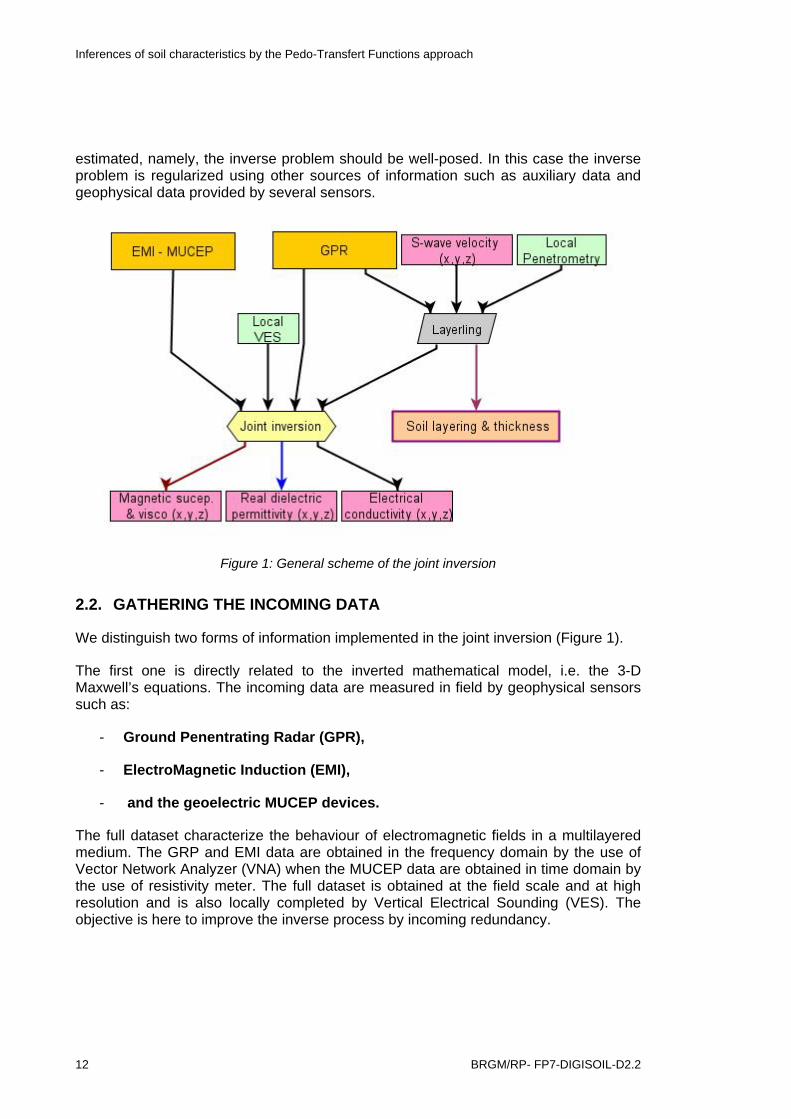
We focus here on the analysis of the joint inversion implemented at the start of the general processing workflow (Figure 1).

The geophysical inverse modeling implemented here consists in finding in an iterative procedure the exact solution of the 3-D Maxwell’s equations for wave propagation in a horizontally multilayered medium. The inverse modeling issues will be then the geophysical constitutive parameters and the geophysical thicknesses of each subsurface layer. The minimization of the objective function is carried out using the global multilevel coordinate search (GMCS) algorithm combined sequentially with the classical Nelder-Mead simplex (NMS) algorithm (Lambot et al., 2002).

It is worth noting that parameter retrieval with inverse modelling will be successful only if enough information is contained in the data with respect to the parameters to be



estimated, namely, the inverse problem should be well-posed. In this case the inverse problem is regularized using other sources of information such as auxiliary data and geophysical data provided by several sensors.

Figure 1: General scheme of the joint inversion

2.2. GATHERING THE INCOMING DATA

We distinguish two forms of information implemented in the joint inversion (Figure 1).

The first one is directly related to the inverted mathematical model, i.e. the 3-D Maxwell’s equations. The incoming data are measured in field by geophysical sensors such as:

- Ground Penentrating Radar (GPR),

- ElectroMagnetic Induction (EMI),

- and the geoelectric MUCEP devices.

The full dataset characterize the behaviour of electromagnetic fields in a multilayered medium. The GRP and EMI data are obtained in the frequency domain by the use of Vector Network Analyzer (VNA) when the MUCEP data are obtained in time domain by the use of resistivity meter. The full dataset is obtained at the field scale and at high resolution and is also locally completed by Vertical Electrical Sounding (VES). The objective is here to improve the inverse process by incoming redundancy.



The second one is related to the auxiliary data. As the soil characteristics of interest, (carbon content, clay content, water content and bulk density) may change with the soil depth, one of the main auxiliary data implemented in the joint inversion is then the soil layering. Afterward, the soil layering will be implicitly expressed on different Figures of the deliverable by the coordinates “x, y and z”.

The layering is characterized by seismic method, and in particular, from the exploitation of surface waves (SASW) dispersion combined with the use of PANDA penetrometer as yet described in deliverables D1.3 and D2.1. Layering is also estimated from geophysical measurements, and then named geophysical layering in reference to the geophysical variability with depth.

2.3. GEOPHYSICAL ISSUES

Following the joint inversion and from the exact solution of the 3-D Maxwell’s equations, three main geophysical parameters are estimated. They concerns (Figure 1):

- the electrical conductivity,

- the dielectric permittivity,

- and the magnetic permeability (or magnetic susceptibility and viscosity). This last one is also obtained directly from magnetism method as described in the deliverable D1.1 (see Annex I, D1.1).

These parameters are obtained at the field scale, at high resolution and for each geophysical layer also estimated by joint inversion. These geophysical parameters are used in the following step of the processing workflow and represent thus the key components from which soil variables are estimated as described afterwards.



3. Conversion of geophysical parameters into soil variables

The estimation of soil variables from geophysical parameters is not straightforward. This work of conversion requires, in some extent, detailed information on all controlling factors.

Empirical or semi-empirical physical laws, largely developed in literature, can be directly applied. This is the case of the well-known equation of Topp et al. (1980) commonly used in literature to convert dielectric permittivity into soil water content.

Others models of conversion require to be parameterized, for instance, from a first calibration performed in laboratory. This is specifically true for electrical conductivity that is dependent on various soil properties (see deliverable D2.1).

We present here the conversion step from geophysical parameters to soil variables. Conversions imply (1) geophysical parameters estimated by joint inversion, i.e. dielectric permittivity, electrical conductivity and magnetic properties and (2) geophysical parameters directly measured in field by geophysical sensors as seismic S-wave velocity and reflectance.

3.1. CONVERSIONS OF GEOPHYSICAL PARAMETER ESTIMATED BY JOINT INVERSION

3.1.1. From dielectric permittivity

The dielectric permittivity is essentially used to estimate the soil water content. Indeed this geophysical parameter is highly influenced and correlated to the soil water content (Huisman et al., 2001; Hilhorst, 1998; Topp et al., 1980). The effects of others soil variables on dielectric permittivity are usually neglected.

As a result, the soil water content can be easily estimated from dielectric permittivity (Figure 2). The relation is generally linear, monotonous and is described by several empirical models such as Topp et al. equation (1980), or Ledieu et al. equation (1986). Theoretical model, CRIM (Complex Refractive Index Model) model based on dielectric mixing, can also be used (Dobson et al., 1985).



Figure 2: Estimation of water content from dielectric permittivity

3.1.2. From electrical conductivity

At the difference to the dielectric permittivity, the interpretation of electrical conductivity remains delicate without regarding all controlling factors. Indeed, the electrical conductivity depends on several chemical and physical soil parameters in complex interaction (Besson, 2007; Besson et al., 2010). For instance, electrical conductivity is highly influenced by water content, clay content, soil salinity, soil temperature and soil structure (Friedman, 2005; Samouelian et al., 2005; Besson et al., 2008). This multi-dependency explains, in some extent, its use for an increasing number of applications in archaeology, hydrogeology, and agriculture as well as soil science in the past decade.

Several models were then developed in the past, to convert the geophysical parameter into soil variables. They are empiric, as the well-known Archie’s law (1942) that relates water saturation degree and porosity to electrical conductivity or semi-empiric as Rhoades model (1989) or Waxman and Smits model (1968) that relate both water saturation degree and salinity to the electrical conductivity. These last ones refer to theoretical considerations on surface and volume electrical conductions that can occur in soils).

In the general framework of the Digisoil processing tool, the use of these models is not excluded. In particular, they enable to estimate soil water content in addition to results of dielectrical conversion as suggested in the previous chapter. These models require, however, an accurate parameterization realized, for instance, by optimization technique from laboratory measurements. We precise also that these models cannot be applied in all soils conditions. This is specifically the case of Archie’s law adapted only to soils close to water saturation and poor in clay content or to highly saline soils (Waxman and Smits, 1968).

In regard to others soil variables of interest as bulk density and clay content, when several authors highlighted the efficiency of electrical conductivity methods to identify bulk density and clay content changes in field (Besson et al., 2004; Seger et al., 2009),



the consecutive empirical relations or correlations cannot be extrapolated without regarding soil conditions.

Consequently a further approach more adapted to the soil conditions of Digisoil experiments is implemented (Figure 3). It consists in data fusion using correlation technique as describe in the deliverable D2.1. Data, gathering both electrical conductivity and values of soil variables, as bulk density and clay content locally measured on soil cores sampled in field, are statistically analyzed. From relations between both variables, empirical models are developed and then used to convert electrical conductivity. Moreover, whatever models implemented, the effect of soil temperature on electrical conductivity is first corrected by the use of Keller and Frischknecht equation (1966).

The issues of this conversion step will be named afterwards “electrical bulk density” and “electrical clay content”.

Figure 3: Estimation of bulk density and clay content from electrical conductivity

3.1.3. From magnetic susceptibility and viscosity

Magnetic property is one of the three issues of the joint inversion. It is also directly measured in field by magnetic method as described in the deliverable D2.1.

The variability of magnetic property may be explained by changes in organic matter content, according to the relation between magnetic properties and iron oxides which result, in some extent, from bacterial activity (Mullins, 1974; Marmet et al., 1999). The relation is not straightforward and is not comforted theoretically.

As a result the approach of data fusion using correlation technique is also applied to estimate carbon content from magnetic susceptibility and viscosity (Figure 4). Carbon content is measured on soil cores sampled in the field. Magnetic property and its consecutive geophysical layer estimated by joint inversion are combined to magnetic property directly measured by magnetic method.



The correlation between magnetic properties and carbon content is analyzed and an empirical relation is developed to express the geophysical parameter into carbon content.

The issue of this conversion step is then named “magnetic carbon content”.

Figure 4: Estimation of carbon content from magnetic susceptibility and viscosity

3.2. CONVERSIONS OF GEOPHYSICAL PARAMETERS MEASURED IN FIELD

3.2.1. From seismic S-wave velocity

Seismic method, as Spectral Analysis of Surface Waves (SASW), leads on the analysis of near surface wave propagation as the transverse propagation (S-wave) in soils.

S-wave velocity was yet used for identifying in situ the soil layering, i.e. the auxiliary data constraining the joint inversion process (see chapter 2.2 of this deliverable). Here, we also use the velocity of S-wave to estimate bulk density. Indeed, the seismic parameter is related to soil bulk density by physical laws as described in the deliverable D2.1.

However these laws require further information on soil structure for correction and validation of the conversion issue. Local measurements of bulk density realized by penetrometer are then combined with S-wave velocity data as shown in Figure 5.

Afterwards the issue of this conversion step is named “seismic bulk density”.



Figure 5: Estimation of bulk density from S-wave velocity

3.2.2. From reflectance

The spectral data, as obtained by hyperspectral remote sensing, is largely influenced by the soil variability in soil organic carbon and clay content (SOC). The literature overview, developed in the deliverable D1.1, highlighted the impact of these “chromophores” on reflectance (Ben-Dor et al., 2002). Several models were then developed to predict organic carbon content and also clay content from reflectance data. The correlations expressed by determination coefficient R² are generally high, up to 0.7 (Stevens et al., 2008).

However, the relationship between a single soil variable of interest and spectra data is not straightforward. The soil spectrum is the result of the overlapping of absorption features of several soil chemical and physical components as, for instance, soil moisture and electrical conductivity (Ben-Dor et al., 2002). As a result, small changes in spectral features due to environmental changes not directly related to SOC or clay content can have negative impact on prediction accuracy.

One of crucial steps in estimating a single soil variable as carbon content or clay content consists then in correcting reflectance to the impact of other factors affecting the spectral data. In particular, soil moisture effect should be erased. In the Digisoil framework, this correction is realized (Figure 6 and Figure 7) from soil water content as the single issue of conversions implying dielectric permittivity (see chapter 3.1.1 of this deliverable).

After correction, the combination of reflectance data to values of soil carbon content and clay content measured on soil cores sampled locally in field is statically analysed. This data fusion using correlation technique results (1) in developing of a conversion model and (2) in estimating soil carbon and clay contents, also named Hyperspectral (Hs) carbon content (Figure 6) and Hs clay content (Figure 7). Estimations in terms of irons oxides and calcium carbonates are also expected from normalized reflectance data.



Figure 6: Estimation of carbon content from reflectance

Figure 7: Estimation of clay content from reflectance



4. Data fusion mapping of the studied soil variables

4.1. DATA FUSION: REDUNDANCY OF ESTIMATES

The main soil variables of interest, i.e. water content, bulk density, clay content and carbon content, can be then estimated from geophysical parameters. These last ones gather (1) dielectric permittivity, electrical conductivity and magnetic properties as the general issues of the joint inversion, (2) and reflectance, seismic S-wave velocity and also magnetic susceptibility directly measured in field.

Different conversion steps lead on estimation of a single soil variable:

• Carbon content can be obtained from conversions that imply both reflectance data and magnetic susceptibility and viscosity.

• Bulk density is predicted by converting both electrical conductivity and S-Wave velocity.

• Clay content is the conversion issue of both electrical conductivity and reflectance data.

• The same for soil water content that is generally obtained from dielectric permittivity but may be also estimated from electrical conductivity.

The redundancy of information for a single soil variable improves the accuracy of the mapping issue after data fusion.

Nevertheless, information is not exactly similar and fully redundant for all variables, but rather further. Indeed, differences may be observed in layering and spatial resolution. This depends on soil sensors used for raw measurements at the field scale. For instance, carbon content from reflectance (Hs carbon content) is estimated for very near-surface of soils whereas carbon content from magnetic properties (Mag carbon content) is estimated for deepest soil layers.

The mapping process aims at integrating all sources of data to an accurate spatial modeling of a single soil variable. This is a fusion strategy for which redundant and further information obtained for each soil variable are combined. The data fusion could be based on fuzzy logic, on multiple regressions or on Bayesian approach as yet described in deliverable D2.1.



4.2. SOIL VARIABLES MAPPING

4.2.1. Water content mapping

Soil water content is mainly estimated from dielectric permittivity (see chapter 3.1.1). The correlation is strong and relatively exclusive. It means that the influence of others factors on the geophysical parameter may be neglected. Consequently, the water content mapping is straightforward without any correction. Its spatial resolution depends on the spatial density of geophysical measurements and on the meshing implemented in the 3D-joint inversion (see chapter 2.1).

Additionally, soil water content is predicted for geophysical layers which are also an estimated issue of the joint inversion.

As a result, soil water content is then mapped in 3D, i.e. for x, y coordinates at the field scale and for z coordinate depending on geophysical layering.

4.2.2. Bulk density mapping

Soil bulk density is given by seismic method and by electric/electromagnetic methods after joint inversion of geophysical raw dataset. Two issues can be used in the mapping process of bulk density, (1) the Seismic bulk density and (2) the Electrical bulk density. Each issue is estimated in space (x, y) and for each soil layer (z).

From combination of two types of information (seismic and electric) on bulk density by using Bayesian approach, a third value of bulk density is obtained and mapped at the field scale and in 3D taking into account the respective uncertainties of the initial seismic and electrical bulk densities (Figure 8).

Figure 8: Fusion mapping of bulk density



4.2.3. Carbon content mapping

Carbon content results in conversions of both reflectance dataset and magnetic properties. The respective issues of conversion, i.e. Hs carbon content and Mag carbon content, are combined in mapping process. This last is relatively similar to the bulk density mapping, based on the Bayesian approach.

Carbon content is then expressed in 3D space (x, y, z) as shown in Figure 9. In further, maps of carbon content and bulk density will be combined to estimate in space carbon stocks (Figure 11).

Figure 9: Fusion mapping of carbon content

4.2.4. Clay content mapping

Clay content values results from electrical conductivity conversion, i.e. electrical clay content, and from reflectance conversion, i.e. Hs clay content.

These data are combined in mapping process, as both for bulk density mapping and clay content mapping, following the process of data fusion mapping (Bayesian, fuzzy).

Clay content is then expressed in 3D space (x, y, z) (Figure 10).

Figure 10: Fusion mapping of clay content



5. Conclusions

This present deliverable concerns the third task of the DIGISOIL’s WP2.

The general workflow implemented in the Digisoil processing tool is detailed from geophysical measurements to the mapping of relevant soil characteristics. The last ones gather soil water content, bulk density, carbon content and clay content. The general processing workflow is summarized in a synthetic scheme (Figure 11).

From geophysical measurements…

Three main processing steps, i.e. the joint inversion step, the conversion step and the mapping step, are then described in the chronological order of data treatments. They are all based on data fusion strategy in view of estimating and mapping with accuracy the soil variables of interest. Indeed, each processing step involves data modeling subjected to quantity of uncertainties in estimates. The data fusion strategy aims then at reducing uncertainties by constraining modeling process in integrating redundant and further information.

Then, the joint inversion is constrained by the combination of measurements obtained by three geophysical sensors. It includes also information on seismic layering used as auxiliary data on soil horizonation.

The conversion step, generally not straightforward, combines geophysical parameters to local information on the relevant soil variables measured in field after sampling.

The mapping process of a single soil variable integrates a set of incoming data proceeding from different geophysical parameters and, hence, conversions. Various techniques of fusion are then used such as Bayesian approach, multiple regressions, correlation technique and fuzzy logic approach. The data fusion is a data assimilation step that can also involve calibration and data correction.

However, several limits and requirements should be investigated.

When we aim at improving the accuracy of estimates by data fusion strategy, the processing way from geophysical measurements to maps of soil variables remains largely not straightforward and, hence, will necessary result in uncertainties on estimates. Calculations of final uncertainties should be realized for each map. This point is challenging and should be further explored.

In addition inadequacy between geophysical layering and soil layering might be observed. Geophysical layering is one of issues of the joint inversion or depends directly on geophysical sensors used as for seismic, magnetic and hyperspectral sensors. Some assumptions could be proposed. For instance, clay content and carbon content estimated from reflectance in near surface could be assumed to be



homogeneous in the entire tilled layer. Indeed agricultural practices as ploughing aim at mixing the soil in the first decimeters. Nevertheless such assumption is largely opened to criticism, in particular for both water content and bulk density which can vary significantly in space in tilled layers as well in the entire soil profile.

The question on the resolution of estimates in depth z can be also posed for the coordinates x and y. When the geophysical issues of the joint inversion, and hence their consecutive soil variables, are spatialized on a similar regular grid defined during inversion process, the spatial resolution of others soil variables converted from seismic, magnetic and hyperspectral data depends directly on the density of geophysical measurements obtained in field. The mapping process should solve the question on spatial resolution of each soil variable by combining incoming data on a single mesh.

Another point concerns the validation of maps realized for each soil variable of interest. Validation step is problematic in regard to the necessity of raising soil sampling in field. Yet the calibration of conversions was based on soil cores sampled in the field. When validation of results requires further samples, it remains dependent on the technical capacity in field. The method of sampling is destructive and time consuming. The soil samples are then obtained only with restricted density.

Digisoil processing tool will be implemented on data measured in validation sites. The issues will consist then in mapping soil variables of interest from geophysical measurements. The four maps obtained will be necessarily comforted by uncertainties on estimates. The topic is complex and will be certainly subjected to various constraints and restrictions. These points will be discussed following results on validation sites (Workpackage 3).

To the pedo-transfer functions approach…

In further work and taking into account the eventual errors on predictions, maps will be integrate in the inference system including the pedo-transfer functions approach (attribute soil inference system). This approach could be implemented to deduce soil properties representative of soil functioning, generally more difficult to measure, from soil variables mapped. In this view, statistical and geostatistical methods could enable not only to estimate properties in space with accuracy but also to analyze their spatial variability in relation with scorpan factors (McBratney et al., 2003) or with all others auxiliary data susceptible to influence the soil functioning as, for instance, climate, human activities, relief, soil management, land covering… (also named soil-related parameters, see Table 1 of the DOW). The general issue of this further work would be then to identify and delineate in space areas of risks as erosion, flood, landslides, compaction… (see Table 2 of the DOW).



Figure 11: Scheme of the general processing workflow



6. References

Archie, G.E. 1942. The electrical resistivity log as an aid in determining some reservoir characteristics. Trans. Am. Inst. Min. Metall. Pet. Eng., 146, 54-62.

Aster R., B. Borchers, C. Thurber, 2005. Parameter estimation and inverse problems. International Geophysics Series. Elsevier, Amsterdam, The Netherlands, 320 pages.

Ben-Dor, E., 2002. Quantitative remote sensing of soil properties. Adv. Agron., 75, 173-243.

Besson A., I. Cousin, A. Samouelian, H. Boizard and G. Richard, 2004. Structural heterogeneity of the soil tilled layer as characterized by 2D electrical resistivity surveying, Soil and Tillage Research, 79, 2, 239–249.

Besson A., 2007. Space and time variability of the soil water content at the field scale as described by the electrical resistivity method. PhD thesis, University Orleans, INRA, Orleans, France, 215 pages.

Besson A., I. Cousin, A. Dorigny, M. Dabas, and D. King. 2008. The temperature correction for the electrical resistivity measurements in undisturbed soil samples: Analysis of the existing conversion models and proposition of a new model. Soil Science, 173, 707-720.

Besson A., I. Cousin, H. Bourennane, B. Nicoullaud, C. Pasquier, G. Richard, A. Dorigny, D. King, 2010. The spatial and temporal organization of soil water at the field scale as described by electrical resistivity measurements. European Journal of Soil Science, 61, 1, 120-132 (13).

Cousin I., A. Besson, H. Bourennane, C. Pasquier, B. Nicoullaud, D. King, G. Richard, 2009. From spatial-continuous electrical resistivity measurements to the soil hydraulic functioning at the field scale. Comptes Rendus Geoscience, 341, 859-867.

Dobson M.C., F.F. Ulaby, M.T. Hallikainen, and M.A. El-Rayes. 1985. Microwave dielectric behavior of wet soil - Part II: Dielectric mixing models. IEEE Transactions on Geoscience and Remote Sensing, 23, 35-46.

Friedman S.P., 2005. Soil properties influencing apparent electrical conductivity: a review. Computers and Electronic in Agriculture, 46, 45-70.

Hilhorst, M.A. 1998. Dielectric characterization of soil, Wageningen Agricultural University, Wageningen, The Netherlands.

Huisman J.A., C. Sperl, W. Bouten, and J.M. Verstraten. 2001. Soil water content measurements at different scales: accuracy of time domain reflectometry and ground penetrating radar. Journal of Hydrology, 245, 48-58.



Keller, G.V., and F.C. Frischknecht. 1966. Electrical methods in geophysical prospecting. Pergamon Press, Oxford

Lambot S., F. André, D. Moghadas, E.C. Slob, H. Vereecken, 2009. Analysis of full-waveform information content in ground penetrating radar and electromagnetic induction data for reconstructing multilayered media, Proceedings of the 2009 5th International Workshop on Advanced Ground Penetrating Radar, 5 pages, IWAGPR 2009, Grenada, Spain, 27-29 May 2009.

Lambot S., E.C. Slob, M. Vanclooster, and H. Vereecken. 2006. Closed loop GPR data inversion for soil hydraulic and electric property determination. Geophysical Research Letters 33:L21405, DOI:10.1029/2006GL027906.

Lambot S., Javaux, M., Hupet, F. and Vanclooster, M., 2002. A global multilevel coordinate search procedure for estimating the unsaturated soil hydraulic properties. Water Resources Research, 38(11): 1224, doi:10.1029/2001WR001224.

Ledieu J., P. Deridder, P. Declerck, S. Dautrebande, 1986. A method of measuring soil-moisture by time-domain reflectometry. Journal of Hydrology, 88, 319-28.

Marmet E., Bina M., Fedroff N., Tabbagh A., 1999, Relationship between human activity and the magnetic properties of soils: a case study in the medieval site of Roissy en France. Archaeological prospection, 6, 161-170.

Mullins C. E., 1974. The magnetic properties of the soils and their application to archaeological prospecting. Archaeophysika, 5, 143 - 347.

Rhoades J. D., N. A. Manteghi, P. J. Shouse and W. J. Alves, 1989. Soil Electrical Conductivity and Soil Salinity: New Formulations and Calibrations. Soil Sci. Soc. Am. J., 53, 433-439.

Samouelian A., I. Cousin, A. Tabbagh, A. Bruand, G. Richard, 2005. Electrical resistivity survey in soil science: a review. Soil and Tillage Research, 83, 173-193.

Seger M., I. Cousin, G. Giot, H. Boizard, F. Mahu and G. Richard, Characterisation of the structural heterogeneity of the soil layer by using in situ 2D and 3D electrical resistivity measurements. ArcheoSciences, 33, 349-351.

Stevens A., B. Van wesemael, H. Bartholomeus, D. Rosillon, B. Tychon, E. Ben-Dor, 2008. Laboratory, field and airborne spectroscopy for monitoring organic carbon content in agricultural soil. Geoderma, 144, 1-2, 395-404.

Tarantola A., 1987. Inverse problem theory : Methods for data fitting and model parameter estimation. Elsevier Science Publishers, Amsterdam, The Netherlands, 333 pages.

Topp G., J.L. Davis, and A.P. Annan. 1980. Electromagnetic Determination of Soil Water Content: Measurements in Coaxial Transmission Lines. Water Resources Research, 16, 574-582.

Vanderborght J., A. Kemna, H. Hardelauf, H. Vereecken, 2005. Potential of electrical resistivity tomography to infer aquifer transport characteristics from tracer studies: A synthetic case study. Water Resources Research, 41, 6: W06013, DOI:10.1029/2004WR003774



Waxman M.H. and L.J.M. Smits, 1968. Electrical conductivities and oil-bearing shaly sands, Soc. Pet. Eng. J., 8, 107–122.

Scientific and Technical Centre RNSC Division

3, avenue Claude-Guillemin - BP 36009 45060 Orléans Cedex 2 – France – Tel.: +33 (0)2 38 64 34 34

inferences of soil characteristics by the pedo- transfert ... · inferences of soil characteristics...

Documents