InferenceSimon Wood

Contents

1 Introduction 21.1 Some examples . . . . . . . . . . . . . . . . . . . . . . . . . . . . . . . . . . . . . . . . . . 21.2 Books and Software . . . . . . . . . . . . . . . . . . . . . . . . . . . . . . . . . . . . . . . 3

2 Likelihood 42.1 The Likelihood Function . . . . . . . . . . . . . . . . . . . . . . . . . . . . . . . . . . . . 4

3 Maximum Likelihood Estimation 63.1 Further examples . . . . . . . . . . . . . . . . . . . . . . . . . . . . . . . . . . . . . . . . 8

4 Numerical likelihood maximization 104.1 Single parameter example . . . . . . . . . . . . . . . . . . . . . . . . . . . . . . . . . . . . 114.2 Vector parameter example . . . . . . . . . . . . . . . . . . . . . . . . . . . . . . . . . . . 134.3 Newton’s method: problems and extensions . . . . . . . . . . . . . . . . . . . . . . . . . . 154.4 Numerical maximization in S . . . . . . . . . . . . . . . . . . . . . . . . . . . . . . . . . . 15

4.4.1 The basics of S . . . . . . . . . . . . . . . . . . . . . . . . . . . . . . . . . . . . . . 154.4.2 Maximizing likelihoods with optim . . . . . . . . . . . . . . . . . . . . . . . . . . . 18

4.5 “Completely Numerical” calculations . . . . . . . . . . . . . . . . . . . . . . . . . . . . . . 19

5 Properties of Maximum Likelihood Estimators 205.1 Invariance . . . . . . . . . . . . . . . . . . . . . . . . . . . . . . . . . . . . . . . . . . . . . 205.2 Properties of the expected log-likelihood . . . . . . . . . . . . . . . . . . . . . . . . . . . 215.3 Consistency . . . . . . . . . . . . . . . . . . . . . . . . . . . . . . . . . . . . . . . . . . . . 235.4 Large sample distribution of θ . . . . . . . . . . . . . . . . . . . . . . . . . . . . . . . . . 245.5 Example . . . . . . . . . . . . . . . . . . . . . . . . . . . . . . . . . . . . . . . . . . . . . . 255.6 What to look for in a good estimator: minimum variance unbiasedness . . . . . . . . . . . 25

6 Hypothesis tests 266.1 The generalized likelihood ratio test (GLRT) . . . . . . . . . . . . . . . . . . . . . . . . . 27

6.1.1 Example: the bone marrow data . . . . . . . . . . . . . . . . . . . . . . . . . . . . 286.1.2 Simple example: Geiger counter calibration . . . . . . . . . . . . . . . . . . . . . . 29

6.2 Why, in the large sample limit, is 2λ ∼ χ2r under H0? . . . . . . . . . . . . . . . . . . . . . 30

6.3 What to look for in a good testing procedure: power etc. . . . . . . . . . . . . . . . . . . . 326.3.1 Power function example . . . . . . . . . . . . . . . . . . . . . . . . . . . . . . . . . 32

7 Interval Estimation 347.1 Intervals based on GLRT inversion . . . . . . . . . . . . . . . . . . . . . . . . . . . . . . . 35

7.1.1 Simple single parameter example: bacteria model . . . . . . . . . . . . . . . . . . . 357.1.2 Multi-parameter example: AIDS epidemic model . . . . . . . . . . . . . . . . . . . 36

7.2 Intervals for functions of parameters . . . . . . . . . . . . . . . . . . . . . . . . . . . . . . 387.3 Intervals based on θ ∼ N(θ0, I−1) . . . . . . . . . . . . . . . . . . . . . . . . . . . . . . . 39

7.3.1 Wald interval example: AIDS again . . . . . . . . . . . . . . . . . . . . . . . . . . 407.4 Induced confidence intervals/ confidence sets . . . . . . . . . . . . . . . . . . . . . . . . . 40

8 Assumptions of the large sample results 40

1

1 Introduction

Consider the situation in which you have some data and a statistical model describing how the datawere generated, but that the model has some parameters the values of which are not known. Parametricstatistical inference is concerned with deciding which values of these parameters are consistent with thedata. This usually involves asking one of three related questions:

1. What value(s) of the parameter(s) are most consistent with the data?

2. Is some specified restriction on the value(s) that the parameter(s) can take consistent with thedata?

3. What range of values of the parameter(s) is consistent with the data?

The methods for answering these questions are known as point estimation, hypothesis testing and intervalestimation, respectively. Usually the statistical model is an attempt to describe the real circumstanceswhich generated the data, and it is hoped that what we learn about the model by statistical inferencetells us something about the reality that the model is trying to describe. Sometimes this hope is wellfounded. In this course we will simply assume that models are correct and develop theory on the basisof this assumption — in other courses you will cover the important topic of model checking.

1.1 Some examples

Thanks to Jim Kay for some of these. . .Point Estimation

• Lightbulbs don’t last for ever and customers and manufacturers need to know how long any par-ticular type of bulb lasts on average, and what the range of lifetimes is. To find out a sample oflightbulbs can be taken and left on until they fail or exceed the available time for the experiment,with the failure times recorded. Assuming that we can write down a probability model for thefailure times (an exponential distribution is not a bad model for tungsten filament bulbs) we wouldwant to find the best estimate of the mean failure time of all bulbs.

• At the beginning of epidemics of new diseases (e.g. HIV/AIDS, SARS, BSE, vCJD) there is oftenconsiderable uncertainty about the underlying rate of increase in new cases of the disease, but it isimportant to try and estimate it. Typically records of the number of new cases will be availableat regular intervals, but these will be quite variable. One simple model of early increase of thedisease says that the number of cases Xi in month ti is a Poisson random variable with meanλi = αeβti , where α is the initial number of cases and β the rate of increase parameter. Given data,what would be the best estimates of these parameters? If we could answer this then short termforecasting would be possible.

Hypothesis testing

• After the Chernobyl nuclear disaster it was necessary to monitor radio-caesium levels in sheepgrazing land. Spot radioactivity measurements are taken at randomly selected points. It is assumedthat the measurements can be treated as observations of a random variable, whose mean correspondsto the overall radio-caesium radioactivity. It is of interest to know whether the observations areconsistent with a mean level at or above the ‘danger’ level, or whether they provide sufficientlystrong evidence that the mean level is below this, that the area can be considered ‘safe’.

• Data were collected at the Ohio State University Bone Marrow Transplant Unit to compare twomethods of bone marrow transplant using 23 patients suffering from non-Hodgkin’s Lymphoma.The patients were each randomly allocated to one of two treatments. The allogenic treatmentconsisted of a transplant from a matched sibling donor. The Autogenic treatment consisted ofremoving the patient’s marrow, ‘cleaning it’ and returning it after a high dose of chemotherapy.For each patient the time of death or relapse is recorded, but for patients who did well, only a

2

time before which the patient had not died or relapsed is recorded (the data are known as ‘rightcensored’).

Treatment Time (Days)Allogenic 28 32 49 84 357 933* 1078* 1183* 1560* 2114* 2144*Autogenic 42 53 57 63 81 140 176 210* 252 476* 524 1037*

Here a * indicates a censored observation (data are from Survival Analysis Klein and Moeschberger).

A reasonable model of these data is that they follow exponential distributions with parameters θl

and θu respectively (mean survival times are 1/θu/l). Medically the interesting question is whetherthe data are consistent with θl = θu or whether separate parameters are required for the two groups.i.e. do the data provide evidence for a difference in survival times between the two groups or not?

Interval Estimation

• Hubble’s law states that the further away a galaxy is the faster it is moving away from us. i.e.if V is velocity (relative to us) and d is distance from us then V = θd. 1/θ is approximately theage of the universe. It is not easy to measure the distance to a galaxy, although its velocity is alittle easier, hence the direct observations of V and d are best viewed as observations of randomvariables the means of which are related by Hubble’s law. Astronomers would like to know whatrange of values of θ are consistent with the observed data, thereby obtaining bounds on the age ofthe universe (Of course there is another school of thought which holds that this quantity is knownexactly, but this is beyond the scope of this course).

• A study examining the cosmetic effects of radiotherapy on women undergoing treatment for earlystage breast cancer examined patients every 4-6 months or so and assessed whether or not theyshowed signs of moderate to severe breast retardation ( termed ‘cosmetic deterioration’). Becauseof the infrequent examination the data consist of interval within which it is known that cosmeticdeterioration set in. For women who showed no deterioration before dying, dropping out or the endof the study, only the time before which there was definitely no deterioration is known.

Time to cosmetic deterioration or censoring (months).(0,7], (0,8], (0,5],(4,11], (5,11], (5,12], (6,10], (7,16], (7,14] (11,15],(11,18], 15*, 17*, (17,25], (17,25],18*, (19,35], (18,26], 22*, 24*, 24*, (25,37], (26,40], (27,34], 32*, 33*, 34*, (36,44], (36,48], 36*, 36*,(37,44], 37*, 37*, 37*, 38*, 40*, 45*, 46*, 46*, 46*, 46*, 46*, 46*, 46*, 46*

(*’s indicate right censored data. The data are from same source as the bone marrow data). Againthe data can be modelled as being observations from an exponential distribution, with mean (1/θ).What range of θ values are consistent with the data — i.e. what is the range of average onset timesthat are consistent with the data?

Note the common theme in all the above examples — we have some data and a model of how thedata were generated which has some parameters of unknown value. In each case we want to know aboutwhich values of the parameters are consistent with the data. This is what parametric statistical inferenceis about.

1.2 Books and Software

Silvey (1975) Statistical Inference, Chapman and Hall and Cox and Hinkley (1974) Theoretical Statistics,Chapman and Hall are both worth a look (and also cover material in subsequent Inference courses).

The S statistical language will be used in these notes. Either the commercial version S-PLUS or thefree version, R, (see cran.r-project.org) should work.

3

2 Likelihood

Who said:

First, we would not accept a treaty that would not have been ratified, nor a treaty that Ithought made sense for the country.

was it (a) Tony Blair, (b) Ronald Reagan or (c) George W. Bush?If you take apart the reasoning behind arriving at an answer it goes something like this: Could it be

Tony Blair? Whatever his failings he can think on his feet and he’s a trained lawyer, it’s improbable thathe would make such a slip, so it’s unlikely to be him. Reagan? Everything was scripted for him and readfrom an auto-cue: unless the auto-cue broke down or he had a really dumb speech writer it’s improbablethat he would have said this, so it’s unlikely to be him. George W. Bush often says things like “Oneyear ago today, the time for excuse-making has come to an end”: it’s quite probable he would say sucha thing, so it’s likely that he is the author of this remark. Of the three possibilities Dubya is the mostlikely.

This type of reasoning lies behind the statistical idea of likelihood. The key idea is as follows. Supposethat we have some data and a probability model describing how the data were generated which has someparameters the values of which are not known . . .

Parameter values which make the data appear relatively probable according tothe model are more likely to be correct than parameter values which make thedata appear relatively improbable according to the model.

Similarly, subject to some caveats covered later, models which make the data appear relatively probableare more likely to be correct than models under which the data appear improbable. By ‘relatively prob-able’ is meant either having a relatively high probability (discrete data), or a relatively high probabilitydensity (continuous data).

To tediously labour the point: in the political quote example, the datum was the quote, the modelwas ‘one of three politicians said it’ and the unknown ‘parameter’ was the name of the politician. Thedata appeared most probable when the parameter took the value ‘George W. Bush’, so this is the mostlikely value of the parameter (and, as it happens, the correct one). Now let’s formalize this idea.

2.1 The Likelihood Function

Suppose you have observations of random variables X1, X2 . . . Xn and can write down their joint p.d.f.or joint p.m.f., f(x1, x2, . . . , xn; θ), where θ is a vector of unknown parameters of the probability modelf . You can simply plug the observed values into f(·) and treat the result as a function of θ alone. Jointp.d.f.s or p.m.f.s with the data plugged in in this way are known as “likelihoods” of the parameters. Theeasiest way to see how it works is to apply the idea to an example.

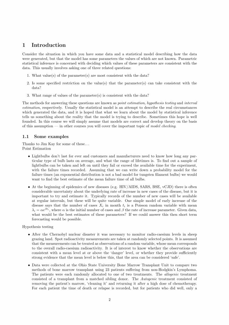
Suppose that we have n data xi which we model as observations of independent random variables Xi

with p.d.f.

f(xi) ={

(β + 1)xβi 0 < xi < 1

0 otherwisewhere β is an unknown parameter. The p.d.f. is shown here for the case β = 2:

−0.5 0.0 0.5 1.0 1.5

0.0

1.0

2.0

3.0

x

f(x)

4

Since the Xi’s are independent, their joint p.d.f. is simply the product of their marginal p.d.f.’s:

f(x1, x2, . . . , xn;β) =n∏

i=1

(β + 1)xβi 0 < xi < 1 for all i

Plugging the observations, xi, (of Xi) into this gives a result that indicates how probable observationsare according to the model. Values of β are not likely to be correct if they cause the model to suggestthat what actually happened is improbable. A value of β which causes the observed data to be probableunder the model is much more likely to be correct (i.e to be the value that actually generated the data).

The joint p.d.f., f(·), with the observed data plugged in and considered as a function of β is calledthe likelihood function (or simply the likelihood) of β:

L(β) =n∏

i=1

(β + 1)xβi

. . . L will be relatively large for likely values of β (values that make the observed data appear relativelyprobable under the model), and small for unlikely values of β (values that make the observed datarelatively improbable according to the model). The most likely value of β is the one that maximises L.Here I have been quite careful to distinguish the dummy variables, xi that are arguments of the jointp.d.f. and the actual observed values xi. Most textbooks are not so careful, and just write xi for both:once you are used to likelihood this doesn’t cause confusion, and usually I won’t bother being so careful.

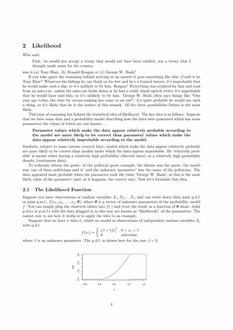
To make the likelihood less abstract, suppose that we have 10 observations (xi’s): 0.68, 0.75, 0.96,0.90, 0.96, 0.62, 0.95, 0.98, 0.73, 0.91. Then we can plot L as a function of β:

0 2 4 6 8 10

020

0040

0060

00

β

L(β)

From the plot . . .

1. What is the most likely value of the β?

2. Is the hypothesis β = 0.1 likely relative to the alternative that β takes some other value?

3. What range of values of β are consistent with the data - i.e. have a reasonable likelihood? Oneway to answer this might be to find the range of values that have a likelihood that is at least 10%of the maximum likelihood.

In the rest of the course we’ll develop well founded formal methods for approaching these types ofquestion using likelihood — at the moment the important thing is to be clear about the basic principles.

5

3 Maximum Likelihood Estimation

Likelihood provides a good general approach to point estimation. Using the magnitude of the likelihoodto judge how consistent parameter values are with the data, the parameter values which maximize thelikelihood function would be judged to be most consistent with the data. Maximum likelihood estimationconsists of finding the values of the parameters that maximize the likelihood and using these as the bestestimates of the parameters. As we have seen, the approach is intuitively appealing, but as we will seelater, it also leads to very general methods with some very good properties.

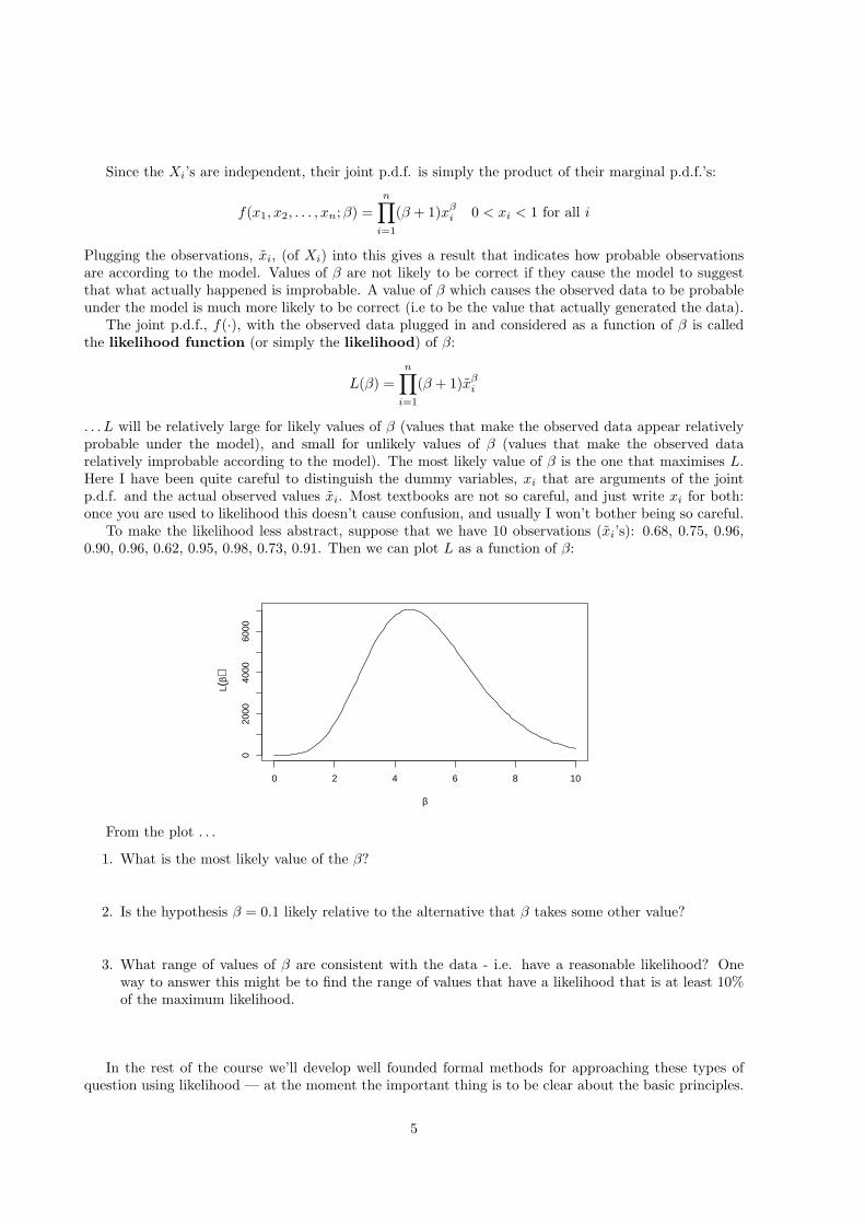
To actually find maximum likelihood estimates we don’t have to resort to plotting L, as was done insection 2.1, but can find the β that maximises L mathematically. As an illustration let’s continue withthe example from section 2.1. The process is made easier if we note that log(L) will be maximised bythe same value of β that maximises L (whichever β gives the biggest L value, must automatically givethe biggest log(L) value). The following plot of log(L) against β illustrates this:

0 2 4 6 8 10

02

46

8

β

log(

L(β)

)

. . . the shape of the plot is very different, but the maximum is at the same value of β. Define l ≡ log(L).Repeated application of the rules log(AB) = log(A) + log(B)∗ and log(Ab) = b log(A) yields:

l(β) = log(L) =n∑

i=1

{log(β + 1) + β log(xi)} = n log(β + 1) + β

n∑

i=1

log(xi)

To find the maximum of l w.r.t. β we need to find the value of β at which dl/dβ = 0.

dl

dβ=

n

β + 1+

n∑

i=1

log(xi)

and setting this to 0 implies that:β = − n∑

log(xi)− 1

Use this expression to obtain the M.L.E. of β from the 10 data given in section 2.1:

In this case the plot of l vs. β makes it clear that the estimate is a maximum likelihood estimate, butoften this should be checked. Differentiating the log-likelihood again yields

d2l

dβ2=

−n

(1 + β)2

∗Which generalizes to:

log

(n∏

i=1

xi

)=

n∑

i=1

log(xi)

6

which is clearly negative at β (or indeed any valid β value) indicating that l(β) is indeed the maximumof the likelihood.

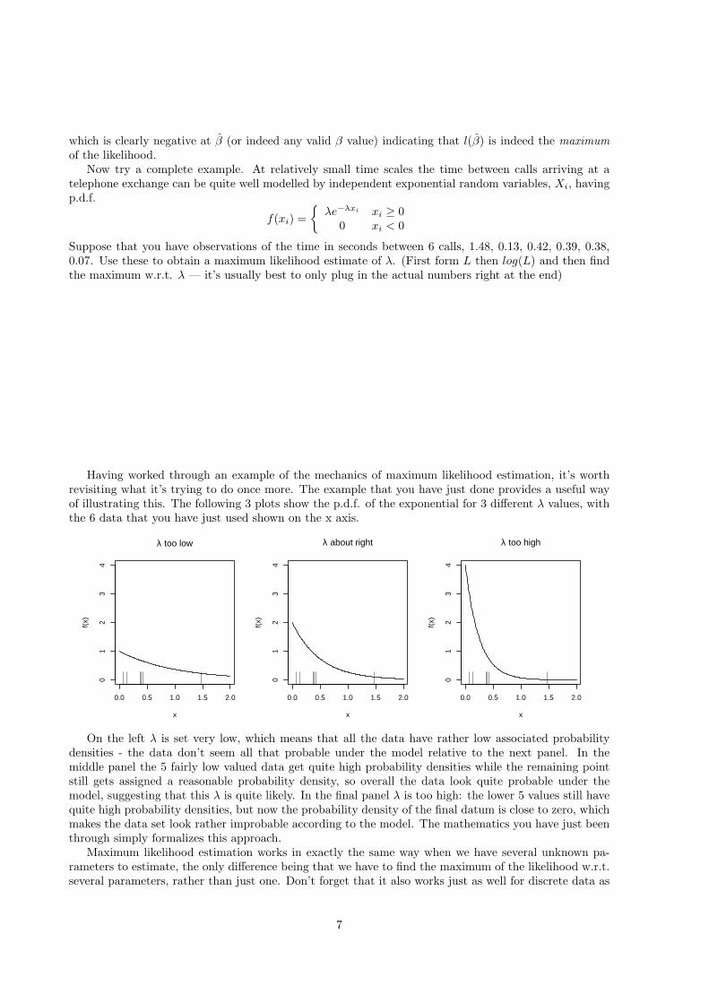
Now try a complete example. At relatively small time scales the time between calls arriving at atelephone exchange can be quite well modelled by independent exponential random variables, Xi, havingp.d.f.

f(xi) ={

λe−λxi xi ≥ 00 xi < 0

Suppose that you have observations of the time in seconds between 6 calls, 1.48, 0.13, 0.42, 0.39, 0.38,0.07. Use these to obtain a maximum likelihood estimate of λ. (First form L then log(L) and then findthe maximum w.r.t. λ — it’s usually best to only plug in the actual numbers right at the end)

Having worked through an example of the mechanics of maximum likelihood estimation, it’s worthrevisiting what it’s trying to do once more. The example that you have just done provides a useful wayof illustrating this. The following 3 plots show the p.d.f. of the exponential for 3 different λ values, withthe 6 data that you have just used shown on the x axis.

0.0 0.5 1.0 1.5 2.0

01

23

4

λ too low

x

f(x)

0.0 0.5 1.0 1.5 2.0

01

23

4

λ about right

x

f(x)

0.0 0.5 1.0 1.5 2.0

01

23

4

λ too high

x

f(x)

On the left λ is set very low, which means that all the data have rather low associated probabilitydensities - the data don’t seem all that probable under the model relative to the next panel. In themiddle panel the 5 fairly low valued data get quite high probability densities while the remaining pointstill gets assigned a reasonable probability density, so overall the data look quite probable under themodel, suggesting that this λ is quite likely. In the final panel λ is too high: the lower 5 values still havequite high probability densities, but now the probability density of the final datum is close to zero, whichmakes the data set look rather improbable according to the model. The mathematics you have just beenthrough simply formalizes this approach.

Maximum likelihood estimation works in exactly the same way when we have several unknown pa-rameters to estimate, the only difference being that we have to find the maximum of the likelihood w.r.t.several parameters, rather than just one. Don’t forget that it also works just as well for discrete data as

7

for continuous data: all that changes is that p.m.f.s take the place of p.d.f.s.

3.1 Further examples

Bone marrow

Now consider again the bone marrow transplant data from section 1.1, concentrating just on the autogenicsample. Recall that a possible model for the time to relapse or death is that the data are observations(possibly censored) of independent exponential random variables, Ti, with p.d.f.

f(ti) = θe−θti , ti ≥ 0.

The value of θ is unknown and must be estimated from the data, but in this case there is no ‘obvious’estimator because some of the data are ‘censored’ observations — we only know that relapse or deathoccurred after some known time. Let u be the set of indices of data that were uncensored (i.e. actualrelapse or death times) and c be the set of indices of data that were censored. We know the p.d.f. forthe uncensored observations, but we also need to find the probabilities for the censored data. These areeasily obtained . . .

Pr[Ti > ti] =∫ ∞

ti

θe−θtdt =[−e−θt

]∞ti

= e−θti

The likelihood is now made up of the product of the joint probability of the censored data and the jointp.d.f. of the uncensored data, under the model. i.e.

L(θ) =∏

i∈u

θe−θti ×∏

i∈c

e−θti

= θnu

n∏

i=1

e−θti

where nu is the number of uncensored observations. As usual it is more convenient to work with thelog-likelihood

l(θ) = nu log(θ)−n∑

i=1

θti

Find the maximum likelihood estimate for θ and evaluate it, given that∑

ti = 3111, and hence obtainthe expected relapse (or death) time.

Applying the same estimator to the allogenic data gives an expected relapse time of about 1912 days —apparently much better, but there is a great deal of variability between individuals in this study, and tobe sure that the apparent difference reflects more than a result of this variability we would need to usethe hypothesis testing methods covered a little later in the course.

8

A two parameter example

So far only single parameter models have been considered, but the method works in the same way formore parameters. As a simple example consider the following 60 year record of mean annual temperaturein New Haven, Connecticut (in ◦F).

49.9 52.3 49.4 51.1 49.4 47.9 49.8 50.9 49.3 51.9 50.8 49.6 49.3 50.6 48.4 50.750.9 50.6 51.5 52.8 51.8 51.1 49.8 50.2 50.4 51.6 51.8 50.9 48.8 51.7 51.0 50.651.7 51.5 52.1 51.3 51.0 54.0 51.4 52.7 53.1 54.6 52.0 52.0 50.9 52.6 50.2 52.651.6 51.9 50.5 50.9 51.7 51.4 51.7 50.8 51.9 51.8 51.9 53.0

A normal probability model may be reasonable for these data. i.e. we could try treating the data asobservations of i.i.d. r.v.s Xi each with p.d.f.

f(xi) =1√2πσ

e−(xi−µ)2

2σ2

where µ and σ are unknown parameters. As usual the log likelihood will be given by:

l(µ, σ) =n∑

i=1

log(f(xi))

that is

l(µ, σ) =n∑

i=1

[− log(

√2π)− log(σ)− (xi − µ)2/(2σ2)

].

As is often the case with log-likelihoods, there is a constant in this expression, −∑log(

√2π), which serves

only to shift the log-likelihood function down by the same amount for all parameter values. Because it isnot affecting the location of the m.l.e., or indeed any aspect of the shape of the log-likelihood function,our results will not be altered at all by simply dropping this term from the log-likelihood. For this reasonconstants which do not depend on the parameters are usually dropped from log-likelihoods, withoutcomment, and the resulting relative log likelihood function is still generally referred to simply as ‘the loglikelihood function’. To save ink, this convention will generally be followed here . . .

l(µ, σ) = −n log(σ)− 12σ2

n∑

i=1

(xi − µ)2.

Maximization of l follows the same approach as in the single parameter case. First differentiate l w.r.t.the parameters,

∂l

∂µ=

1σ2

n∑

i=1

(xi − µ)

∂l

∂σ= −n

σ+

1σ3

n∑

i=1

(xi − µ)2

then set both the resulting expressions to zero and solve the resulting pair of simultaneous equations forµ and σ:

9

We must also check that the estimates are maximum likelihood estimates. This involves evaluatingthe second derivative matrix, or Hessian, of l w.r.t. the parameters at µ, σ. That is

H =

(∂2l∂µ2

∂2l∂µ∂σ

∂2l∂σ∂µ

∂2l∂σ2

)∣∣∣∣∣µ,σ

=( − n

σ2 − 2σ3

∑(xi − µ)

− 2σ3

∑(xi − µ) n

σ2 − 3σ4

∑(xi − µ)2

)∣∣∣∣µ,σ

=( − n

σ2 00 −2n

σ2

).

For the turning point at µ, σ to be a maximum requires that H is negative definite — that is all itseigenvalues must be negative. The eigen-values of a diagonal matrix are the elements on the diagonal†

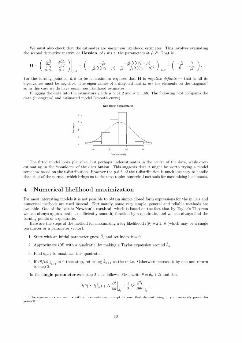
so in this case we do have maximum likelihood estimates.Plugging the data into the estimators yields µ ' 51.2 and σ ' 1.58. The following plot compares the

data (histogram) and estimated model (smooth curve).

New Haven Temperatures

Temperature (F)

Fre

quen

cy

48 50 52 54

05

1015

20

The fitted model looks plausible, but perhaps underestimates in the centre of the data, while over-estimating in the ‘shoulders’ of the distribution. This suggests that it might be worth trying a modelsomehow based on the t-distribution. However the p.d.f. of the t-distribution is much less easy to handlethan that of the normal, which brings us to the next topic: numerical methods for maximizing likelihoods.

4 Numerical likelihood maximization

For most interesting models it is not possible to obtain simple closed form expressions for the m.l.e.s andnumerical methods are used instead. Fortunately, some very simple, general and reliable methods areavailable. One of the best is Newton’s method, which is based on the fact that by Taylor’s Theoremwe can always approximate a (sufficiently smooth) function by a quadratic, and we can always find theturning points of a quadratic.

Here are the steps of the method for maximizing a log likelihood l(θ) w.r.t. θ (which may be a singleparameter or a parameter vector).

1. Start with an initial parameter guess θ0 and set index k = 0.

2. Approximate l(θ) with a quadratic, by making a Taylor expansion around θk.

3. Find θk+1 to maximize this quadratic.

4. If ∂l/∂θ|θk+1≈ 0 then stop, returning θk+1 as the m.l.e. Otherwise increase k by one and return

to step 2.

In the single parameter case step 2 is as follows. First write θ = θk + ∆ and then

l(θ) ' l(θk) + ∆∂l

∂θ

∣∣∣∣θk

+12∆2 ∂2l

∂θ2

∣∣∣∣θk

.

†The eigenvectors are vectors with all elements zero, except for one, that element being 1: you can easily prove thisyourself.

10

Differentiating w.r.t. ∆ gives∂l

∂∆' ∂l

∂θ

∣∣∣∣θk

+ ∆∂2l

∂θ2

∣∣∣∣θk

while setting the differential to zero and solving yields

∆ = −(

∂2l

∂θ2

∣∣∣∣θk

)−1∂l

∂θ

∣∣∣∣θk

which maximizes the quadratic approximation to l. Hence step 3 is

θk+1 = θk + ∆.

For vector parameters in general, step 2 is

l(θ) ' l(θk) + ∆T g +12∆T H∆

where θ = θk + ∆,

g =

∂l∂θ1

∣∣∣θk

∂l∂θ2

∣∣∣θk

.

.

and H =

∂2l∂θ2

1

∣∣∣θk

∂2l∂θ1∂θ2

∣∣∣θk

. .

∂2l∂θ1∂θ2

∣∣∣θk

∂2l∂θ2

2

∣∣∣θk

. .

. . . .

. . . .

.

Differentiating w.r.t. each element of ∆ results in

∂l∂∆1∂l

∂∆2

.

.

= g + H∆.

Setting each of these derivatives to zero and solving the resulting system of equations gives

∆ = −H−1g

as the maximizer of the quadratic approximation to the log-likelihood. Hence in this case step 3 amountsto

θk+1 = θk −H−1g.

4.1 Single parameter example

As an example of using Newton’s method to maximize a likelihood in the single parameter case, consideran experiment on anti-biotic efficacy. A 1 litre culture of 5×105 cells (this figure known quite accurately)is set up and dosed with antibiotic. After 2 hours and every subsequent hour up to 14 hours after dosing0.1ml of the culture is removed and the live bacteria in this sample counted under a microscope. Thedata are:

Sample hour, ti 2 3 4 5 6 7 8 9 10 11 12 13 14Live bacteria count, yi 35 33 33 39 24 25 18 20 23 13 14 20 18

A simple model for the sample counts, yi, is that their expected value is

E(Yi) = 50e−δti ,

11

where δ is an unknown ‘death rate’ parameter (per hour) and ti is the sample time in hours. Giventhe sampling protocol, it is reasonable to assume that the actual counts are observations of independentPoisson random variables with this mean. The parameter δ must be estimated. Note that this exampleis different in kind from the bone marrow survival example — the main source of variability in this caseis the sampling and not the random timing of individual deaths (because the population is so large inthis case).

Writing µi ≡ E(Yi), we have that the probability function for Yi is

f(yi) =µyi

i e−µi

yi!where µi = 50e−δti .

Therefore the log likelihood is

l(δ) =n∑

i=1

[yi log(µi)− µi − log(yi!)]

Dropping the δ independent constant∑

log(yi!) and substituting in the model for µi gives

l(δ) =n∑

i=1

yi[log(50)− δti]−n∑

i=1

50e−δti .

The derivatives are then∂l

∂δ= −

n∑

i=1

yiti +n∑

i=1

50tie−δti

and∂2l

∂δ2= −50

n∑

i=1

t2i e−δti .

The presence of the ti term in e−δti makes it impossible to find a closed form solution for ∂l/∂δ = 0, sonumerical methods are required here.Exercise Given that

∑yi = 315,

∑ti = 104,

∑yiti = 2192 and

∑t2i = 1014, and starting from a guess

δ0 = 0, apply one step of Newton’s method to obtain δ1.

In fact it only takes 4 steps of Newton’s algorithm to maximize the likelihood as the following plotshows. In each panel the continuous curve is the log likelihood, and the dashed curve is the quadraticapproximation obtained by expanding the log-likelihood around the point marked •. As the iterationsprogress you can see how the maximum of the quadratic approximation gets closer to the maximum ofthe log-likelihood, until they eventually coincide. It follows of course that the δk become ever closer tothe m.l.e. as iteration progresses.

12

0.00 0.05 0.10 0.15 0.20 0.25

550

600

650

700

δ

l(δ)

δ1 = 0.059

0.00 0.05 0.10 0.15 0.20 0.25

550

600

650

700

δ

l(δ)

δ2 = 0.088

0.00 0.05 0.10 0.15 0.20 0.25

550

600

650

700

δ

l(δ)

δ3 = 0.094

0.00 0.05 0.10 0.15 0.20 0.25

550

600

650

700

δ

l(δ)

δ4 = 0.094

4.2 Vector parameter example

Now consider an example with a vector parameter. The following data are reported AIDS cases inBelgium in the early stages of the epidemic there.

Year (19—) 81 82 83 84 85 86 87 88 89 90 91 92 93New cases 12 14 33 50 67 74 123 141 165 204 253 246 240

One important question early in such epidemics is whether control measures are beginning to havean impact, or whether the disease is continuing to spread essentially unchecked. A simple model forunchecked growth leads to an ‘exponential increase’ model (similar in structure to the bacteria model).The model says that the number of cases, yi, are observations of independent Poisson r.v.s, with expectedvalues

µi = αeβti

where ti is the number of years since 1980. Proceeding broadly as in the bacteria example leads to a loglikelihood

l(α, β) =n∑

i=1

yi[log(α) + βti]−n∑

i=1

αeβti

so the gradient vector is (∂l/∂α∂l/∂β

)=

( ∑yi/α−∑

exp(βti)∑yiti − α

∑ti exp(βti)

)

and the Hessian is (∂2l∂θ2

1

∂2l∂θ1∂θ2

∂2l∂θ1∂θ2

∂2l∂θ2

2

)=

( −∑yi/α2 −∑

tieβti

−∑tie

βti −α∑

t2i eβti .

)

A swift glance at the expression for the gradients should be enough to convince you that numericalmethods will be required to find the m.l.e.s of the parameters. Starting from an initial guess α0 = 4,

13

β0 = .35, here is the first Newton iteration.(

α0

β0

)=

(4

.35

)⇒ g =

(88.43721850.02

), H =

( −101.375 −3409.25−3409.25 154567

)

⇒ H−1g =( −1.820

0.028

)

⇒(

α1

β1

)=

(α0

β0

)−H−1g =

(5.820.322

)

After a number of further iterations the likelihood is maximized at α = 23.1, β = 0.202. The followingfigure illustrates the first 6 steps of the Newton method for this case. In each panel the continuouslabelled contours show the log likelihood. The dashed unlabelled contours (which are at the same levelsas the continuous) show the quadratic approximation to the likelihood based on the Taylor expansionat the point •. The maximum of the approximating quadratic is shown as ◦ in each case, and the truemaximum is marked with a point.

α

β

0 10 20 30 40 50 60 70

0.0

0.1

0.2

0.3

0.4

0 10 20 30 40 50 60 70

0.0

0.1

0.2

0.3

0.4

α1 = 5.82, β1 = 0.322

α

β

0 10 20 30 40 50 60 70

0.0

0.1

0.2

0.3

0.4

0 10 20 30 40 50 60 70

0.0

0.1

0.2

0.3

0.4

α2 = 8.64, β2 = 0.285

α

β

0 10 20 30 40 50 60 70

0.0

0.1

0.2

0.3

0.4

0 10 20 30 40 50 60 70

0.0

0.1

0.2

0.3

0.4

α3 = 11.9, β3 = 0.259

α

β

0 10 20 30 40 50 60 70

0.0

0.1

0.2

0.3

0.4

0 10 20 30 40 50 60 70

0.0

0.1

0.2

0.3

0.4

α4 = 15.84, β4 = 0.233

α

β

0 10 20 30 40 50 60 70

0.0

0.1

0.2

0.3

0.4

0 10 20 30 40 50 60 70

0.0

0.1

0.2

0.3

0.4

α5 = 19.44, β5 = 0.216

α

β

0 10 20 30 40 50 60 70

0.0

0.1

0.2

0.3

0.4

0 10 20 30 40 50 60 70

0.0

0.1

0.2

0.3

0.4

α6 = 22.01, β6 = 0.206

The original data with the curve giving the expected cases per year according to the estimate modelis shown here . . .

1982 1984 1986 1988 1990 1992

5010

015

020

025

0

AIDS cases in Belgium

Year

New

AID

S c

ases

14

The fit doesn’t look too bad, but the points are perhaps not scattered around the curve as much as youwould expect if the differences between data and model were no more than random variability — perhapsthe exponential model was too pessimistic and a model which showed some slowing down would be bettersupported by the data (but perhaps, with 13 data, this is over-interpretation).

4.3 Newton’s method: problems and extensions

For a likelihood that is continuous to second derivative and has a maximum within the allowable parameterspace, Taylor’s theorem guarantees that Newton’s method will find that maximum provided the initialparameter estimates are close enough to the m.l.e.. Unfortunately ‘close enough’ varies from problemto problem. If the initial estimates are too far from the m.l.e. then the Newton iteration can diverge,with estimates actually getting further from the m.l.e. Furthermore, if the log-likelihood is an awkwardshape then it can happen that the Hessian is not negative definite over some regions of parameter space,and hence the quadratic approximation has no unique maximum. In fact both divergence and indefiniteHessians can occur for the AIDS model log-likelihood shown in the previous section, if the initial parameterguess is unfortunate.

In practice two simple steps usually prevent these problems leading to actual failure. The first is totreat ∆ not as defining the step to take, but merely as defining the direction in the parameter space alongwhich to search for better parameter values. Evaluating the log-likelihood at a few locations along ∆,from θk, usually locates parameter values with higher likelihood, even if stepping all the way to θk + ∆would decrease the likelihood. The second step only comes into play if the first fails (e.g. if the Hessianis indefinite — i.e. some of its eigenvalues are positive): in this case one can treat g as the direction inwhich to search for better parameters. Unless the m.l.e. has already been located, a sufficiently smallstep in this direction is guaranteed to increase the likelihood.

Given that Newton type methods will almost always be performed by computer, a possible ‘enhance-ment’ is to estimate the required derivatives numerically, rather than working out exact expressions forthem. For an appropriate choice of small interval h,

∂l

∂θ' l(θ + h)− l(θ)

h

and equivalent formulae can be obtained for second derivatives. With careful choice of h these finitedifference approximations can be very accurate. For example, if l can be calculated to 14 significantfigures, then the derivative can usually be obtained to 7 significant figures.

Newton type methods based on finite difference approximate derivatives can be very effective, but onlyif finite difference intervals h are very carefully chosen . . . a topic best left to experts. Fortunately, thereare plenty of expert implementations freely available, which make it easy to maximize most likelihoodswithout having to calculate any derivatives for yourself, as we shall now see.

4.4 Numerical maximization in S

The S statistical computing language has built in routines for numerical maximization of likelihoods (orany other function, in fact). To use these facilities you need to spend a little time learning some new things,and revising some old things about the language. There are two implementations of S in widespread use.S-PLUS is the commercial implementation and is available in the labs here. R (cran.r-project.org) isa free version written by university statisticians: it tends to be a faster and some of its facilities, includingthose for maximization, are arguably a bit better than the S-PLUS versions.

4.4.1 The basics of S

S stores all data and variables in named objects. You create objects by assigning a value to them using theassignment operator <-. Here are some examples. Anything written after a # character is a comment.

a<-1 # create a variable ‘a’ with value 1a<-3.5 # give ‘a’ the value 3.5

15

b<-c(1,3.1,4.7) # create an array called ‘b’ with elements 1, 3.1 and 4.7b[2]<- -1.3 # assign the second element of ‘b’ the value -1.3d<-1:4 # create an array ‘d’ of length 4 containing 1,2,3,4M<-matrix(0,3,2) # create a 3 row, 2 column matrix of 0’s called MM[3,1]<-2 # assign 3rd row of column 1 of M the value 2M[2,]<-c(3,1) # set the second row of M to values 3,1M[,2]<-b # set the second column of M to the values in b

To see what is contained in an object, simply type its name. For example

> M<-matrix(1:6,2,3)> M

[,1] [,2] [,3][1,] 1 3 5[2,] 2 4 6

where > is the S ‘command prompt’ (indicates that S is waiting for you to type in a command).Sometimes it is useful to create objects known as lists, which are simple named lists of other objects.

For example, following on from the previous examples

my.list<-list(vec=b,mat=M) # create a list called ‘my.list’

would create a list containing 2 items vec is an array of the 3 numbers that were in b and mat is a copy ofthe matrix M. The items in the list are accessed by using the list name followed by a $ character followedby the item name. For example my.list$vec.

Array arithmetic works almost as it does in Minitab, except that no let command is needed and= is replaced by <-. Here are some examples, with the results printed too.

> a<-1:3> b<-a/2 # divide each element of a by 2> b[1] 0.5 1.0 1.5> d<-a*b # multiply arrays a and b element by element - result in d> d[1] 0.5 2.0 4.5> d<-a^2*exp(b) # d_i = a_i^2 exp(b_i) for i=1..3> d[1] 1.648721 10.873127 40.335202

Matrix arithmetic is also straightforward. For example if M is an n×n matrix and b is an n-vector(i.e. an array of length n) then

y<-M%*%bqf.1<-t(b)%*%M%*%bx<-solve(M,b)qf.2<-t(b)%*%solve(M,b)

form y = Mb, QF1 = bT Mb, x = M−1b and QF2 = bT M−1b respectively. %*% performs matrixmultiplication, t() transposes a matrix and solve(M,b) forms M−1b (by solving Mx = b for x).

Functions are one of the real strengths of S. Hundreds of built-in functions are available for performingall sorts of data manipulation and statistical tasks, but you can also write your own functions (e.g. loglikelihood functions). solve(), t() and matrix() are examples of functions that have already been usedabove. Functions have a name, take arguments supplied between brackets () and return an object ofsome sort as a result, which you can assign to a named object if you wish (if you don’t assign the resultof a function to something then it will usually be printed and will then be lost). Some functions don’treturn an object, but produce a ‘side-effect’ such as a plot. Here are some useful functions

16

> a<-1:4 # create array 1,2,3,4> s.a<-sum(a) # sum the array and store result in ‘s.a’> s.a # print value of ‘s.a’[1] 10> prod(a) # use prod() function to form product of elements of a[1] 24> dpois(a,4) # probability of elements of a if Poi(4) r.v.s[1] 0.07326256 0.14652511 0.19536681 0.19536681> ppois(a,3) # Pr[A<=a] if A~Poi(3) using function for c.d.f of Poi[1] 0.1991483 0.4231901 0.6472319 0.8152632

More complicated functions may have many possible arguments, most of which have default values whichthey will take if you don’t specify a value. For example the plot() function can take optional argumentsxlab, ylab and main for the axes labels and titles, but will simply use its own defaults if you don’t supplyany. e.g.

x.a<-1:20;y.a<-x+rnorm(20) # simulate straight line data with N(0,1) errorsplot(x.a,y.a) # plot with default annotationplot(x.a,y.a,xlab="x",ylab="y",main="A plot about nothing") # plot with annotation

Notice how the later arguments have been supplied in the form name=something — the naming ofarguments lets you supply some arguments and omit others without confusing S.

Writing your own functions is straightforward. Suppose that you want to write a function calledmy.func which will take two parameters b1 and b2, say, two n-vectors x and y and form

n∑

i=1

xb1i exp(−b2yi)

here is how to do it . . .

my.func<-function(b,x,y) # create a function ‘my.func’ defined by code between { and }{ res<-sum(x^b[1]*exp(-b[2]*y)) # calculate required quantity

res # return value}

Once created the function can be called like any other. For example:

b<-c(1.5,1);x<-runif(20);y<-runif(20) # create test datamy.func(b,x,y)

Here’s the function in action . . .

> b<-c(1.5,1);x<-runif(20);y<-runif(20) # create test data> my.func(b,x,y) # call function[1] 4.783403

Of course the following would work just as well:

> params<-c(1.5,1);x.data<-runif(20);response<-runif(20)> my.func(b=params,x=x.data,y=response)[1] 4.783403

and for this simple function we don’t have to use the argument names: my.func(params,x.data,response)would also have worked.

Help is available by typing ? followed by the function you want help with. e.g. ?plot.

17

4.4.2 Maximizing likelihoods with optim

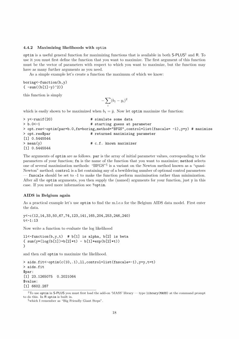
optim is a useful general function for maximizing functions that is available in both S-PLUS‡ and R. Touse it you must first define the function that you want to maximize. The first argument of this functionmust be the vector of parameters with respect to which you want to maximize, but the function mayhave as many further arguments as you need.

As a simple example let’s create a function the maximum of which we know:

boring<-function(b,y){ -sum((b[1]-y)^2)}

this function is simply−

∑

i

(b1 − yi)2

which is easily shown to be maximized when b1 = y. Now let optim maximize the function:

> y<-runif(20) # simulate some data> b.0<-1 # starting guess at parameter> opt.res<-optim(par=b.0,fn=boring,method="BFGS",control=list(fnscale= -1),y=y) # maximize> opt.res$par # returned maximizing parameter[1] 0.5445544> mean(y) # c.f. known maximizer[1] 0.5445544

The arguments of optim are as follows. par is the array of initial parameter values, corresponding to theparameters of your function; fn is the name of the function that you want to maximize; method selectsone of several maximization methods: “BFGS”§ is a variant on the Newton method known as a “quasi-Newton” method; control is a list containing any of a bewildering number of optional control parameters— fnscale should be set to -1 to make the function perform maximisation rather than minimization.After all the optim arguments, you then supply the (named) arguments for your function, just y in thiscase. If you need more information see ?optim.

AIDS in Belgium again

As a practical example let’s use optim to find the m.l.e.s for the Belgium AIDS data model. First enterthe data.

y<-c(12,14,33,50,67,74,123,141,165,204,253,246,240)t<-1:13

Now write a function to evaluate the log likelihood

ll<-function(b,y,t) # b[1] is alpha, b[2] is beta{ sum(y*(log(b[1])+b[2]*t) - b[1]*exp(b[2]*t))}

and then call optim to maximize the likelihood.

> aids.fit<-optim(c(10,.1),ll,control=list(fnscale=-1),y=y,t=t)> aids.fit$par:[1] 23.1265075 0.2021064$value:[1] 6602.287

‡To use optim in S-PLUS you must first load the add-on ‘MASS’ library — type library(MASS) at the command promptto do this. In R optim is built in.

§which I remember as “Big Friendly Giant Steps”.

18

Notice how simple this is — there is not even any need to calculate derivatives. As we will see shortly,the Hessian matrix at the m.l.e.s is often required when using likelihood, but optim will also return anestimate of this for you, if you set its argument hessian to TRUE. Although not required, it is possible tosupply derivatives to optim, and if this is done the algorithm will usually converge more quickly and theestimated Hessian will be more accurate.

4.5 “Completely Numerical” calculations

Sometimes the likelihood itself is actually difficult or tedious to write down explicitly. For example, sincethere is no closed form expression for the integral of the normal p.d.f. we cannot write down an explicitexpression for the likelihood for interval data on normal r.v.s. Similarly the expression for the p.d.f.of a t-distribution is unpleasantly complicated. However, S and other statistics packages have built infunctions for evaluating many p.d.f.s and c.d.f.s, including the c.d.f. for the normal and the p.d.f. forthe t-distribution. As a consequence it is very straightforward to write an S function to evaluate thelog-likelihood in such cases, even though the likelihood may be awkward to write down.

To illustrate this point let’s return to the New Haven temperature data from section 3.1, but trymodelling them with a t-distribution, which puts more probability in the tails of the distribution thanthe normal. To motivate the model, first note that the original model could have been re-written as

Zi =Xi − µ

σ∼ N(0, 1).

Standard transformation theory tells us that if the p.d.f. of Zi is fz(zi) then the p.d.f. of Xi will befz((xi − µ)/σ)/σ, which written out in full is the normal p.d.f. used in section 3.1.

To try and overcome the deficiencies of the original model let’s try the model

Zi =Xi − µ

σ∼ tm

where m is the degrees of freedom of the t-distribution. If ft,m is the p.d.f. of the t-distribution with mdegrees of freedom, then standard transformation theory says that the p.d.f. of Xi is now

fx(xi) = ft,m((xi − µ)/σ)/σ

so that the log-likelihood is

l(σ, µ, m) =n∑

i=1

log(fx(xi))

which is easily evaluated in S. A suitable function is:

logL<-function(b,x,df) # df is m{ z<-(x-b[1])/exp(b[2]) # transform data. b[1] is mu, exp(b[2]) is sigma

sum(log(dt(z,df=df)/exp(b[2]))) # sum the logs of the p.d.f. of x}

where b[2] is the log of σ — a trick to ensure that the estimate of σ cannot become negative. m/df hasnot been included in the parameter array b because it is a discrete parameter, and optim only deals withcontinuous parameters. To find the m.l.e. for m, optim can simply be called for a range of m values, andthe one resulting in the highest maximized likelihood chosen. A few trials soon established that m = 8.

Here is the S code to maximize the likelihood and plot the results.

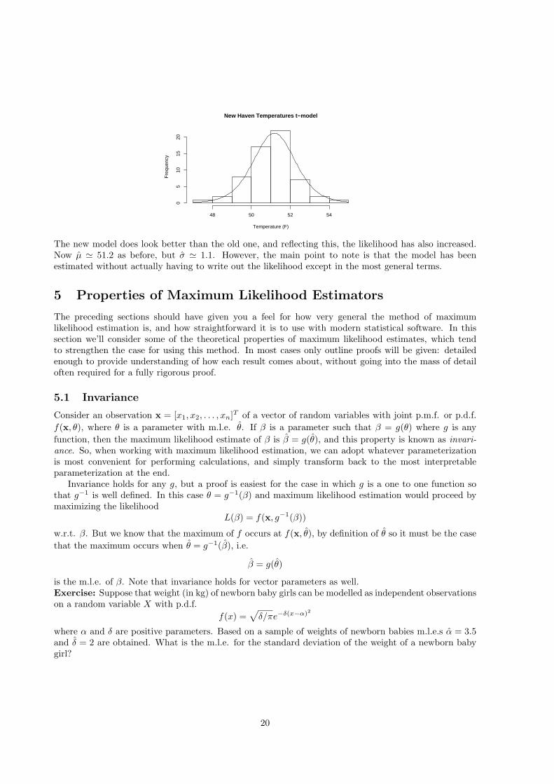
b<-optim(c(50,log(2)),logL,control=list(fnscale=-1),df=8,x=nhtemp)mu.hat<-b$par[1];sigma.hat<-exp(b$par[2]) # extract estimateshist(nhtemp,xlab="Temperature (F)",main="New Haven Temperatures t-model")temp<-seq(47,55,length=200) # sequence of temperatures to predict overlines(temp,n*dt((temp-mu.hat)/sigma.hat,df=8)/sigma.hat)

19

New Haven Temperatures t−model

Temperature (F)

Fre

quen

cy

48 50 52 54

05

1015

20

The new model does look better than the old one, and reflecting this, the likelihood has also increased.Now µ ' 51.2 as before, but σ ' 1.1. However, the main point to note is that the model has beenestimated without actually having to write out the likelihood except in the most general terms.

5 Properties of Maximum Likelihood Estimators

The preceding sections should have given you a feel for how very general the method of maximumlikelihood estimation is, and how straightforward it is to use with modern statistical software. In thissection we’ll consider some of the theoretical properties of maximum likelihood estimates, which tendto strengthen the case for using this method. In most cases only outline proofs will be given: detailedenough to provide understanding of how each result comes about, without going into the mass of detailoften required for a fully rigorous proof.

5.1 Invariance

Consider an observation x = [x1, x2, . . . , xn]T of a vector of random variables with joint p.m.f. or p.d.f.f(x, θ), where θ is a parameter with m.l.e. θ. If β is a parameter such that β = g(θ) where g is anyfunction, then the maximum likelihood estimate of β is β = g(θ), and this property is known as invari-ance. So, when working with maximum likelihood estimation, we can adopt whatever parameterizationis most convenient for performing calculations, and simply transform back to the most interpretableparameterization at the end.

Invariance holds for any g, but a proof is easiest for the case in which g is a one to one function sothat g−1 is well defined. In this case θ = g−1(β) and maximum likelihood estimation would proceed bymaximizing the likelihood

L(β) = f(x, g−1(β))

w.r.t. β. But we know that the maximum of f occurs at f(x, θ), by definition of θ so it must be the casethat the maximum occurs when θ = g−1(β), i.e.

β = g(θ)

is the m.l.e. of β. Note that invariance holds for vector parameters as well.Exercise: Suppose that weight (in kg) of newborn baby girls can be modelled as independent observationson a random variable X with p.d.f.

f(x) =√

δ/πe−δ(x−α)2

where α and δ are positive parameters. Based on a sample of weights of newborn babies m.l.e.s α = 3.5and δ = 2 are obtained. What is the m.l.e. for the standard deviation of the weight of a newborn babygirl?

20

5.2 Properties of the expected log-likelihood

The key to proving and understanding the large sample properties of maximum likelihood estimatorslies in obtaining some results for the expectation of the log-likelihood and then using the convergence inprobability of the log-likelihood to its expected value which results from the law of large numbers. Inthis section, some simple properties of the expected log likelihood are derived.

Let x1, x2, . . . , xn be independent observations from a p.d.f. f(x, θ) where θ is an unknown parameterwith true value θ0. Treating θ as unknown, the log-likelihood for θ is

l(θ) =n∑

i=1

log[f(xi, θ)] =n∑

i=1

li(θ)

where li is the log-likelihood given only the single observation xi. Treating l as a function of randomvariables X1, X2, . . . , Xn means that l is itself a random variable (and the li are independent randomvariables). Hence we can consider expectations of l and its derivatives.

Result 1:

E0

(∂l

∂θ

∣∣∣∣θ0

)= 0

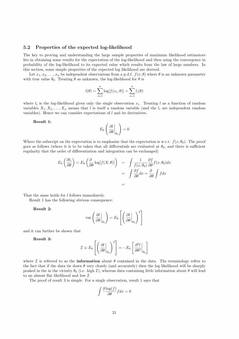
Where the subscript on the expectation is to emphasize that the expectation is w.r.t. f(x, θ0). The proofgoes as follows (where it is to be taken that all differentials are evaluated at θ0, and there is sufficientregularity that the order of differentiation and integration can be exchanged)

E0

(∂li∂θ

)= E0

(∂

∂θlog[f(X, θ)]

)=

∫1

f(x, θ0)∂f

∂θf(x, θ0)dx

=∫

∂f

∂θdx =

∂

∂θ

∫fdx

=

That the same holds for l follows immediately.Result 1 has the following obvious consequence:

Result 2:

var

(∂l

∂θ

∣∣∣∣θ0

)= E0

(∂l

∂θ

∣∣∣∣θ0

)2

and it can further be shown that

Result 3:

I ≡ E0

(∂l

∂θ

∣∣∣∣θ0

)2 = −E0

[∂2l

∂θ2

∣∣∣∣θ0

]

where I is referred to as the information about θ contained in the data. The terminology refers tothe fact that if the data tie down θ very closely (and accurately) then the log likelihood will be sharplypeaked in the in the vicinity θ0 (i.e. high I), whereas data containing little information about θ will leadto an almost flat likelihood and low I.

The proof of result 3 is simple. For a single observation, result 1 says that∫

∂ log(f)∂θ

fdx = 0

21

Differentiating again w.r.t. θ yields∫

∂2 log(f)∂θ2

f +∂ log(f)

∂θ

∂f

∂θdx

but∂ log(f)

∂θ=

1f

∂f

∂θ

and so

which is

E0

[∂2li∂θ2

∣∣∣∣θ0

]= −E0

(∂li∂θ

∣∣∣∣θ0

)2

The result follows very easily (given the independence of the li).Now notice that result 1 says that the expected log likelihood has a turning point at θ0, while since I

is non-negative, result 3 indicates that this turning point is a maximum. So the expected log likelihoodhas a maximum at the true parameter value. Unfortunately results 1 and 3 don’t establish that thismaximum is the global maximum of the expected log likelihood, but a slightly more involved proof showsthat this is in fact the case.

Result 4: E0[l(θ0)] ≥ E0[l(θ)] ∀ θ

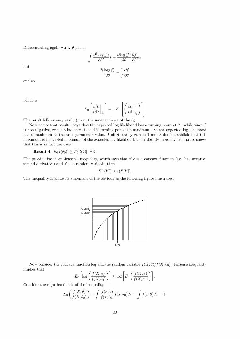
The proof is based on Jensen’s inequality, which says that if c is a concave function (i.e. has negativesecond derivative) and Y is a random variable, then

E[c(Y )] ≤ c(E[Y ]).

The inequality is almost a statement of the obvious as the following figure illustrates:

E(Y)

C[E(Y)]

E(C[Y])

Now consider the concave function log and the random variable f(X, θ)/f(X, θ0). Jensen’s inequalityimplies that

E0

[log

(f(X, θ)f(X, θ0)

)]≤ log

[E0

(f(X, θ)f(X, θ0)

)].

Consider the right hand side of the inequality.

E0

(f(X, θ)f(X, θ0)

)=

∫f(x, θ)f(x, θ0)

f(x, θ0)dx =∫

f(x, θ)dx = 1.

22

So, since log(1) = 0 the inequality becomes

E0

[log

(f(X, θ)f(X, θ0)

)]≤ 0

⇒ E0[log(f(X, θ))] ≤ E0[log(f(X, θ0))]

from which the result follows immediately.The above results were derived for continuous X, but also hold for discrete X: the proofs are almost

identical, but with∑

all xireplacing

∫dx. Note also that although the results presented here were derived

assuming that the data were independent observations from the same distribution, this is in fact muchmore restrictive than is necessary, and the results hold more generally. Similarly the results generalizeimmediately to vector parameters. In this case result 3 is:

Result 3 (vector parameter)

I ≡ E0

(∂l

∂θ1

)2∂l

∂θ1

∂l∂θ2

.

∂l∂θ2

∂l∂θ1

(∂l

∂θ2

)2

.

. . .

= −E0

∂2l∂θ2

1

∂2l∂θ1∂θ2

.∂2l

∂θ2∂θ1

∂2l∂θ2

1.

. . .

(1)

5.3 Consistency

Maximum likelihood estimators are often not unbiased, but under quite mild regularity conditions theyare consistent. This means that as the sample size on which the estimate is based tends to infinity, themaximum likelihood estimator tends in probability to the true parameter value. Consistency thereforeimplies asymptotic¶ unbiasedness, but it actually implies slightly more than this — for example that thevariance of the estimator is decreasing with sample size.

Formally if θ0 is the true value of parameter θ and θn is its m.l.e. based on n observations x1, x2, . . . , xn

then consistency means thatPr[|θn − θ0| < ε] → 1

as n →∞ for any positive ε.To see why m.l.e.s are consistent, consider an outline proof for the case of a single parameter, θ, esti-

mated from independent observations x1, x2, . . . , xn on a random variable with p.m.f. or p.d.f. f(x, θ0).The log-likelihood in this case will be

l(θ) ∝ 1n

n∑

i=1

log(f(xi, θ))

where the factor of 1/n is introduced purely for later convenience. We need to show that in the largesample limit l(θ) achieves its maximum at the true parameter value θ0, but in the previous section itwas shown that the expected value of the log likelihood for a single observation attains its maximumat θ0. The law of large numbers tells us that as n → ∞,

∑ni=1 log[f(Xi, θ)]/n tends (in probability) to

E0[log(f(X, θ))]. So in the large sample limit we have that

l(θ0) ≥ l(θ)

i.e. that θ is θ0.To show that θ → θ0 in some well ordered manner as n →∞ requires that we assume some regularity

(for example we need at least to be able to assume that if θ1 and θ2 are ‘close’ then so are l(θ1) andl(θ2)), but in the vast majority of practical situations such conditions hold. A picture can help illustratehow the argument works:¶‘asymptotic’ here meaning ‘as sample size tends to infinity’.

23

θ0θ

E0(log(f(X, θ)))1

n∑i=1

nlog(f(xi, θ))

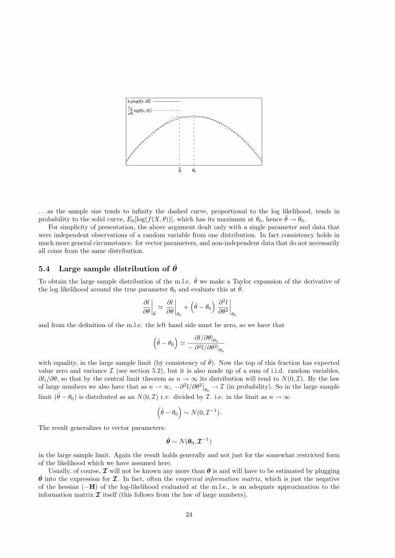
. . . as the sample size tends to infinity the dashed curve, proportional to the log likelihood, tends inprobability to the solid curve, E0[log(f(X, θ))], which has its maximum at θ0, hence θ → θ0.

For simplicity of presentation, the above argument dealt only with a single parameter and data thatwere independent observations of a random variable from one distribution. In fact consistency holds inmuch more general circumstance: for vector parameters, and non-independent data that do not necessarilyall come from the same distribution.

5.4 Large sample distribution of θ

To obtain the large sample distribution of the m.l.e. θ we make a Taylor expansion of the derivative ofthe log likelihood around the true parameter θ0 and evaluate this at θ.

∂l

∂θ

∣∣∣∣θ

' ∂l

∂θ

∣∣∣∣θ0

+(θ − θ0

) ∂2l

∂θ2

∣∣∣∣θ0

and from the definition of the m.l.e. the left hand side must be zero, so we have that

(θ − θ0

)' ∂l/∂θ|θ0

− ∂2l/∂θ2|θ0

with equality, in the large sample limit (by consistency of θ). Now the top of this fraction has expectedvalue zero and variance I (see section 5.2), but it is also made up of a sum of i.i.d. random variables,∂li/∂θ, so that by the central limit theorem as n →∞ its distribution will tend to N(0, I). By the lawof large numbers we also have that as n →∞, −∂2l/∂θ2

∣∣θ0→ I (in probability). So in the large sample

limit (θ − θ0) is distributed as an N(0, I) r.v. divided by I. i.e. in the limit as n →∞(θ − θ0

)∼ N(0, I−1).

The result generalizes to vector parameters:

θ ∼ N(θ0,I−1)

in the large sample limit. Again the result holds generally and not just for the somewhat restricted formof the likelihood which we have assumed here.

Usually, of course, I will not be known any more than θ is and will have to be estimated by pluggingθ into the expression for I. In fact, often the empirical information matrix, which is just the negativeof the hessian (−H) of the log-likelihood evaluated at the m.l.e., is an adequate approximation to theinformation matrix I itself (this follows from the law of large numbers).

24

5.5 Example

In an experiment designed to assess the mean lifetime of a batch of lightbulbs, 100 were selected atrandom and left on for 1000 hours or until they failed, whichever was the shorter. At the end of theexperiment 90 bulbs were still alight and 10 had failed. The failure times (in hours) were:

11 51 59 118 168 257 263 396 485 933

A reasonable model for the failure times Ti is that they are observations of exponential random variableswith p.d.f.

f(ti) = λe−λti

The likelihood of λ is the product of the joint p.d.f. of the 10 observed failure times and the probabilityof the 90 other bulbs lasting more than 1000 hours, i.e.

L(λ) =10∏

i=1

λe−λti ×100∏

i=11

e−λ1000

leading to a log likelihood

l(λ) = 10 log(λ)− λ

(10∑

i=1

ti + 90000

).

Differentiating gives∂l

∂λ=

10λ−

10∑

i=1

ti − 90000,∂2l

∂λ2=−10λ2

.

Setting ∂l/∂λ = 0 ⇒ λ = 10/(∑

ti + 90000) = 10/(92741) = 1.078× 10−4. It follows by invariance thatthe m.l.e. of the mean failure time is 1/λ = 9274.1.

From the large sample distributional results it follows that the approximate standard deviation of λis given by

σλ '(−E

[∂2l

∂λ2

])−1/2

=λ√10

which is estimated as λ/√

10 ' 0.341×10−4. Indeed since the large sample results say that the distributionof λ is approximately normal, we can set approximate 95% confidence limits on λ of

1.08± 1.96× .34× 10−4 = (0.41× 10−4, 1.75× 10−4).

This corresponds to a 95% confidence interval for the mean lifetime of (5726, 24178) (obtained by takingthe reciprocal of the confidence limits on λ). What two changes could you make to the study in order tonarrow this interval?

Note that while confidence intervals calculated in this way are usually acceptable, they do have somestrange properties. For example if we had parameterized the likelihood in terms of the mean lifetimethen, by invariance, the m.l.e. for the mean lifetime would have come out exactly as before, but theconfidence interval would not. i.e. confidence intervals calculated in this manner are not invariant —instead, the answer you get depends on the parameterization you choose to use. This seems somewhatunsatisfactory, and we will see later how the situation can be improved.

5.6 What to look for in a good estimator: minimum variance unbiasedness

How should we judge how good an estimation procedure is? One important theoretical result which helpsis the Cramer-Rao lower bound on the variance of an unbiased estimator. Let θ be a parameter andθ an unbiased estimator of θ, meaning that E(θ) = θ. The Cramer-Rao result says that the variance

25

of θ can not be smaller than I−1 - the inverse of the information about θ (I−1 in the vector parametercase)‖. This result offers rather strong support for the method of maximum likelihood estimation, for aswe have seen, in the large sample limit m.l.e.’s are unbiased and have exactly I−1 variance.

6 Hypothesis tests

Suppose that you have data x1, x2, . . . , xn and a probability model with unknown parameters θ describinghow these data were generated. Further suppose that you have some preconceived notion of the valuesthat the parameters might take, or more generally some restrictions on the values that they might take,and that you want to test this null hypothesis (H0) against some alternative hypothesis (H1)about the values that the parameters can take. In the situation described, a likelihood function can bewritten down for θ and it seems natural to use this likelihood to compare the relative plausibility of thehypotheses.

Generally hypotheses fall into two main classes. Simple hypotheses completely specify the values takenby the parameters. For example, in a single parameter problem H0 : θ = 2.5 is an example of a simplehypothesis. Composite hypotheses are hypotheses that allow the parameter(s) to take a range of possiblevalues. For example, in a one parameter problem H1 : θ > 2.5 is an example of a composite hypothesis— a range of θ values are consistent with it. A two parameter example of a composite hypothesis isH0 : θ1 = θ2 — there is a range of values of θ1 and θ2 satisfying the hypothesis.

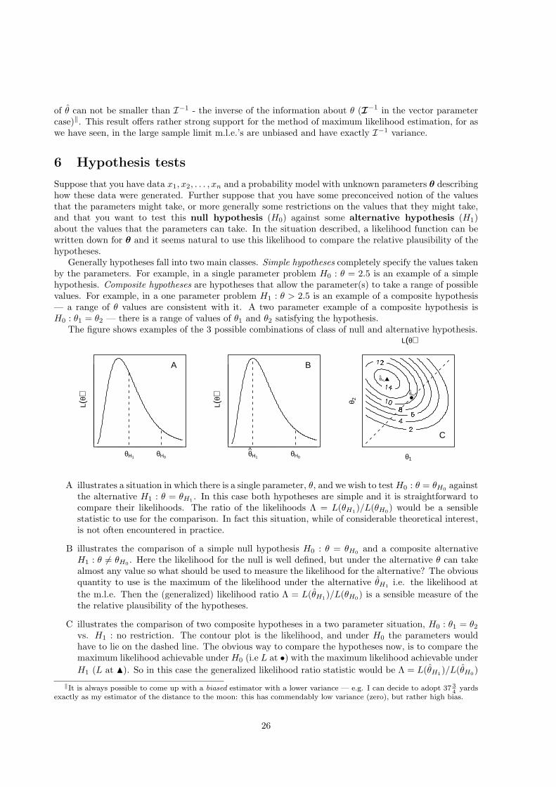
The figure shows examples of the 3 possible combinations of class of null and alternative hypothesis.

L(θ)

θH0θH1

A

L(θ)

θH0θH1

B

L(θ)

θ1

θ 2

θH1

θH0

C

A illustrates a situation in which there is a single parameter, θ, and we wish to test H0 : θ = θH0 againstthe alternative H1 : θ = θH1 . In this case both hypotheses are simple and it is straightforward tocompare their likelihoods. The ratio of the likelihoods Λ = L(θH1)/L(θH0) would be a sensiblestatistic to use for the comparison. In fact this situation, while of considerable theoretical interest,is not often encountered in practice.

B illustrates the comparison of a simple null hypothesis H0 : θ = θH0 and a composite alternativeH1 : θ 6= θH0 . Here the likelihood for the null is well defined, but under the alternative θ can takealmost any value so what should be used to measure the likelihood for the alternative? The obviousquantity to use is the maximum of the likelihood under the alternative θH1 i.e. the likelihood atthe m.l.e. Then the (generalized) likelihood ratio Λ = L(θH1)/L(θH0) is a sensible measure of thethe relative plausibility of the hypotheses.

C illustrates the comparison of two composite hypotheses in a two parameter situation, H0 : θ1 = θ2

vs. H1 : no restriction. The contour plot is the likelihood, and under H0 the parameters wouldhave to lie on the dashed line. The obvious way to compare the hypotheses now, is to compare themaximum likelihood achievable under H0 (i.e L at •) with the maximum likelihood achievable underH1 (L at N). So in this case the generalized likelihood ratio statistic would be Λ = L(θH1)/L(θH0)

‖It is always possible to come up with a biased estimator with a lower variance — e.g. I can decide to adopt 37 34

yardsexactly as my estimator of the distance to the moon: this has commendably low variance (zero), but rather high bias.

26

In each testing situation some variation on the generalized likelihood ratio statistic provides a rea-sonable measure of the relative plausibility of the hypotheses, with ‘high’ values supporting H1 and ‘low’values supporting H0. At first sight it might seem appropriate to simply accept H1 if Λ > 1 and H0

otherwise, but there are two reasons why this is not done.

1. In many situations there is some prior reason to favour H0. Often it is favoured because it is thesimpler hypothesis, and we would like to have the simplest model consistent with the data∗. Inother circumstances there may be more pressing considerations: for example in a radioactive con-tamination monitoring programme it makes sense to accept the null hypothesis that contaminationis at dangerous levels, unless the data provide strong evidence to the contrary.

2. Usually the null hypothesis states that the data were generated by a more restricted version of themodel assumed under the alternative hypothesis. In this circumstance it is always the case thatL(θH1) ≥ L(θH0) ⇒ Λ ≥ 1, and in fact Λ > 1 almost surely. Hence accepting H1 if Λ > 1 wouldmean (almost) always accepting H1, even if H0 is true†.

For these reasons it is usual to accept H0 unless Λ is so large that, in effect, the evidence against H0 hasbecome too strong to ignore. The null hypothesis is presumed true until it is proven otherwise beyondreasonable doubt. The strength of the evidence against H0 (and for H1) is judged using a p-value.

The p-value is the probability of the test statistic taking a value at least as favourable to H1

as that actually observed, if H0 is true.

Learn this and understand it. The p-value is an attempt to measure the consistency of the data with thenull hypothesis.

1. Low p-values imply that the data are improbable if H0 is true. Since the data actually happened,this suggests rejecting H0 in favour of H1.

2. High p-values suggest that the data are quite probable under H0: since data and hypothesis appearconsistent, H0 is accepted.

How low should a p-value be in order to cause rejection of H0? There is no ‘correct’ answer to this, andmany statisticians prefer not to make one up, simply quoting the p-value instead. If a value, α, is chosen,such that H0 will be rejected if the p-value is ≤ α then α is known as the significance level of the test.Traditional choices for α are 0.05, 0.01, 0.005 and 0.001, with 0.05 being the most common.

The usefulness of p-values as a measure of the evidence against H0 stems from their general applica-bility: a p-value of 0.04 has the same meaning whatever hypothesis is being tested and whatever methodis being used for the test and that meaning is well defined.

6.1 The generalized likelihood ratio test (GLRT)

Sometimes it is possible to find the exact distribution of Λ (or more usually λ = log Λ), and hence calculatea p-value exactly. But in most circumstances it is not possible and we have to use approximate p-valuesbased on large sample results. Fortunately a very general result exists for the log of the generalizedlikelihood ratio test statistic.

Consider an observation x on a random vector of dimension n with p.d.f. (or p.m.f.) f(x,θ), whereθ is a parameter vector. Suppose that we want to test

H0 : R(θ) = 0 vs. H1 : R(θ) 6= 0

where R is a vector valued function of θ such that H0 imposes r restrictions on the parameter vector. IfH0 is true then in the limit as n →∞

2λ = 2(l(θH1)− l(θH0)) ∼ χ2r (2)

∗This approach fits well some quite well accepted ideas in the philosophy of science.†This argument applies for any test statistic, not just Λ.

27

where l is the log-likelihood function, θH1 is the m.l.e. of θ and θH0 is the value of θ satisfying R(θ) =0 which maximizes the likelihood (i.e. the restricted m.l.e.). This result is the basis for calculatingapproximate p-values.

6.1.1 Example: the bone marrow data

Recall the bone marrow transplant survival data from section 1.1 . . .Treatment Time (Days)Allogenic 28 32 49 84 357 933* 1078* 1183* 1560* 2114* 2144*Autogenic 42 53 57 63 81 140 176 210* 252 476* 524 1037*

The data are times ti from treatment to relapse or death, except for the data marked *, which areobservations that ti > t∗i . The medically interesting question is whether these data provide evidencethat the average relapse rate differs between the groups (equivalently, that the mean relapse time differsbetween the groups). A possible model for these data is that

f(ti) =

θale−θalti ti > 0 & Allogenic group

θaue−θauti ti > 0 & Autogenic group0 otherwise

where the parameters θau and θal are the ‘relapse rates’ for each group. To test the medical questionstatistically we can test

H0 : θau = θal versus H1 : θau 6= θal

using a generalized likelihood ratio test. To calculate the test statistic we must find the maximizedlikelihood under each of the two hypotheses. Following section 3.1 the log likelihood is

l(θau, θal) = nau,uc log(θau)− θau

∑au group

ti + nal,uc log(θal)− θal

∑

al group

ti

and this must be maximized to find θH1 (the uc subscript indicates ‘uncensored’). Under the restrictionimposed by H0 we can replace all occurrences of θau and θal in the log likelihood by a single parameterθ ≡ θau = θal, in which case we could simplify the log likelihood to

l(θ) = nuc log(θ)− θ∑

all cases

ti.

The likelihood under H0 must also be maximized to find θH0 .As we saw in section 3.1 we could maximize these log- likelihoods by hand calculation, but following

the principle that you shouldn’t waste brain power on something you can more easily get a machine todo, we can also use optim in S. I’ll enter the censored data as negative numbers, so that they can easilybe identified, and then ignore the sign when calculating the log likelihood. I’ll also get optim to maximizethe likelihoods w.r.t. the logs of the θs — invariance says that this is legitimate and it will ensure thatthe θ estimates come out positive, as they should. So the data are entered as . . .

allo<-c(28 , 32 , 49 , 84 , 357 , -933 , -1078 , -1183 , -1560 , -2114 , -2144)auto<-c(42 , 53 , 57 , 63 , 81 , 140 , 176 , -210 , 252 , -476 , 524 , -1037)

and here is a function suitable for calculating the log likelihood under H1 and H0 (depending on whetherit is supplied with a single parameter or a 2-vector).

bm.ll<-function(p,allo,auto)# work out bone marrow log-lik. Code censored obs. as -ve{ p<-exp(p) # optimize w.r.t log(theta) since theta +ve

n.al.uc<-sum(allo>0) # number uncensored for allon.au.uc<-sum(auto>0) # number uncensored for autoif (length(p)==1) theta.au<-theta.al<-p # under H_0

28

else {theta.au<-p[1];theta.al<-p[2]} # under H_1ll<-n.au.uc*log(theta.au) - theta.au*sum(abs(auto)) + # the log-likelihood

n.al.uc*log(theta.al) - theta.al*sum(abs(allo))}

It is now straightforward to evaluate l(θH1), l(θH0), λ and hence the p-value.

> m1<-optim(c(-7,-7),bm.ll,control=list(fnscale=-1),method="BFGS",allo=allo,auto=auto)> m0<-optim(-7,bm.ll,control=list(fnscale=-1),method="BFGS",allo=allo,auto=auto)> lambda<-m1$value-m0$value> p.value<-1-pchisq(2*lambda,df=1);p.value[1] 0.001699133

(pchisq(x,df=r) returns Pr[X ≤ x] where X ∼ χ2r.) So there is quite strong evidence to reject the null

here: the treatments really differ here.What do the results tell us? Under H1 the m.l.e.s of the parameters are (0.0029, 0.0005) and under H0:

(0.0011, 0.0011). So the data suggest that the experimental treatment has a higher relapse rate, and thehypothesis test indicates that this difference is real. It also looks clinically significant so the new treatmentdoes not look like a good prospect when the other treatment is possible. (The conventional treatmentrequires that a matched donor can be found and that they undergo a painful operation themselves, toextract the donated marrow. This is not always possible.)

6.1.2 Simple example: Geiger counter calibration

A Geiger counter (radioactivity meter) is calibrated using a source of known radioactivity. The countsrecorded by the counter, xi, over 200 1 second intervals are recorded . . .

8 12 6 11 3 9 9 8 5 4 6 11 6 14 3 5 15 11 7 6 9 9 14 136 11 . . . . . . . . . . . . . . . . . . . . . . 9 8 5 8 9 14 14

The sum of the counts∑200

i=1 xi = 1800. The counts can be treated as observations of i.i.d. Poi(θ) r.v.s.with p.m.f.

f(xi, θ) =θxie−θ

xi!xi ≥ 0, θ ≥ 0.

If the Geiger counter is functioning correctly then θ = 10, and to check this we would test

H0 : θ = 10 versus H1 : θ 6= 10.

Suppose that we choose to test at a significance level of 5% (i.e. H0 will be rejected if the p-value is≤ 0.05). The test can be performed using a generalized likelihood ratio test. The log likelihood is

l(θ) = log(θ)n∑

i=1

xi − nθ

(where I have simply dropped the θ-independent constant∑

log(xi!)).In this case H0 completely specifies the value of θ, so the m.l.e. under H0 is 10, and the maximized

log likelihood under H0 is simply

l(10) = log(10)n∑

i=1

xi − n× 10 = 2144.653

29

Find the maximum of the log likelihood under H1.

Now calculate the log likelihood ratio test statistic 2λ.

Given that a χ21 r.v. has a 5% chance of being greater than or equal to 3.84, would you accept or reject

H0? What does this imply about the Geiger counter?

Finally, given the form of the m.l.e., what was the point of recording the counts in 200 1 - second intervalsrather than recording the count in 1 200 second interval?

6.2 Why, in the large sample limit, is 2λ ∼ χ2r under H0?

To simplify matters, first suppose that the parameterization is such that θ =(

ψγ

)where ψ is r

dimensional and the null hypothesis can be written H0 : ψ = ψ0. In principle it is always possible tore-parameterize a model so that the null has this form‡.

Now let the unrestricted m.l.e. be(

ψγ

)and

(ψ0

γ0

)be the m.l.e. under the restrictions defining

the null hypothesis. The key to making progress is to be able to express γ0 in terms of ψ, γ and ψ0.This is possible in general in the large sample limit, provided that the null hypothesis is true, so that ψis close to ψ0. Taking a Taylor expansion of the log likelihood around the unrestricted m.l.e. θ yields

l(θ) ' l(θ)− 12

(θ − θ

)T

H(θ − θ

)(3)

where Hi,j = − ∂2l/∂θi∂θj

∣∣θ. Exponentiating this expression the likelihood can be written

L(θ) ' L(θ) exp[−

(θ − θ

)T

H(θ − θ

)/2

].

i.e. the likelihood can be approximated by a function proportional to the p.d.f. of an N(θ,H−1) randomvariable. Now it is a standard result from probability that if part of θ is fixed in the normal p.d.f. thenthe remainder of θ has a normal p.d.f., but with a different mean. Specifically if

(ψγ

)∼ N

((ψγ

),

(Σψψ Σψγ

Σγψ Σγγ

))

‡Of course, to use the result no re-parameterization is necessary — it’s only being done here for theoretical conveniencewhen deriving the result.

30

then the conditional mean isE(γ|ψ) = γ + ΣγψΣ−1

ψψ(ψ − ψ).

and hence the conditional likelihood will be approximately gaussian in form with this conditional meanas the gaussian mean. Since we know that the normal p.d.f. (Gaussian) attains its maximum at its meanit follows that the m.l.e. for γ given that ψ = ψ0 must be

γ0 ' γ + ΣγψΣ−1ψψ(ψ0 − ψ). (4)

If the null hypothesis is true then in the large sample limit ψ → ψ0 (in probability) so that the approxi-mate likelihood tends to the true likelihood and we can expect (4) to hold for the maximizers of the exactlikelihood.

Expressing (4) in terms of a partitioning of Σ = H−1, is not as useful as having the results in termsof the equivalent partitioning of H itself. Writing ΣH = I in partitioned form,

(Σψψ Σψγ

Σγψ Σγγ

) (Hψψ Hψγ

Hγψ Hγγ

)=

(I 00 I

),

and multiplying out, results in four matrix equations of which two are useful:

ΣψψHψψ + ΣψγHγψ = I (5)

ΣψψHψγ + ΣψγHγγ = 0. (6)

Re-arranging (6) while noting that by symmetry HTψγ = Hγψ and ΣT

ψγ = Σγψ§, yields

−H−1γγ Hγψ = ΣγψΣ−1

ψψ

and henceγ0 = γ + H−1

γγ Hγψ(ψ −ψ0). (7)

For later use it’s also worth eliminating Σψγ from (5) and (6), which results in

Σ−1ψψ = Hψψ −HψγH−1

γγ Hγψ. (8)

Now provided that the null hypothesis is true, so that ψ is close to ψ0, we can re-use the expansion (3)and write the log-likelihood at the restricted m.l.e. as

l(ψ0, γ0) ' l(ψ, γ)− 12

(ψ0 − ψγ0 − γ

)T

H(

ψ0 − ψγ0 − γ

).

Hence

2λ = 2(l(ψ, γ)− l(ψ0, γ0)) '(

ψ0 − ψγ0 − γ

)T

H(

ψ0 − ψγ0 − γ

).

Substituting for γ0 from (7) and writing out H in partitioned form gives

2λ '(

ψ0 − ψ

H−1γγ Hγψ(ψ −ψ0)

)T (Hψψ Hψγ

Hγψ Hγγ

)(ψ0 − ψ

H−1γγ Hγψ(ψ −ψ0)

)

and a short routine slog results in

2λ ' (ψ −ψ0)T[Hψψ −HψγH−1

γγ Hγψ

](ψ −ψ0).

But given (8), this means that2λ ' (ψ −ψ0)T Σ−1

ψψ(ψ −ψ0) (9)

§and of course remembering that (AB)T = BT AT .

31

Now if H0 is true then as n →∞ this expression will tend towards exactness as ψ → ψ0. Furthermore,by the law of large numbers and (1), H → I as n → ∞ (recall that in this section H is the negativesecond derivative matrix), which means that Σ tends to I−1, and hence Σψψ tends to the covariancematrix of ψ (see section 5.4). Hence by the asymptotic normality of the m.l.e. ψ

2λ ∼ χ2r

Having proved the asymptotic distribution of λ you might at this point be wondering why it was worthbothering when we could simply have used the right hand side of (9) directly as the test statistic. Thisapproach is indeed possible and is known as the Wald test, but it suffers from the disadvantage thatat finite sample sizes the magnitude of the test statistic depends on how we choose to parameterize themodel. The GLRT on the other hand is invariant to the parameterization we choose to use, irrespectiveof sample size. This invariance seems much more satisfactory — we don’t generally want our statisticalconclusions to depend on details of how we set the model up which could never be detected by observingdata from the model.

6.3 What to look for in a good testing procedure: power etc.

In testing procedures in which a significance level is chosen and the null hypothesis is either accepted orrejected, two errors are possible.

1. A Type I error is rejection of the null hypothesis when it is true.

2. A Type II error is acceptance of the null hypothesis when it is false.¶

A good testing procedure should keep the probabilities of both types of error low, but there is a trade-offbetween keeping the type I error probability low and keeping the type II error probability low. Generallya test procedure which tries to avoid falsely rejecting H0 will require a great deal of evidence in order toreject H0 — but this is bound to lead to a quite high probability of not rejecting H0 when it is false.

To move beyond generalities error probabilities must be calculated. By construction of p-values, theprobability of a type one error is simply the significance level of a test. For example, when testing atthe 5% level we reject H0 whenever the test statistic is as supportive of H1 as will only be seen in 5% ofdatasets generated under H0: this means that we will reject H0 for 5% of datasets for which it is true.

So the probability of a type I error is set by the chosen significance level, which suggests that given achoice of testing procedures we should select the one that gives the lowest probability of a type II errorgiven our chosen significance level. Since 1 − Pr[Type II error] is the probability of correctly rejectingthe null when it is false, it is known as the power of a test. So at a given significance level, we wouldgenerally choose the most powerful test available: this principle is often referred to as the Neyman-Pearsonapproach to hypothesis testing.

If both hypotheses are simple then the power is usually quite easy to calculate, and it is then possibleto prove that the most powerful test will always be based on the likelihood ratio test statistic. Althoughderived only for simple hypotheses, this result, known as the Neyman-Pearson lemma, provides partof the theoretical support for using the generalized likelihood ratio test statistic.

In most interesting cases H1 is not simple and then the power depends on the true parameter values:in this circumstance it is usual to calculate the power function for the test procedure. The followingsimple example illustrates the principle.

6.3.1 Power function example

An often overlooked consequence of globalization is that many dragons can now only find work providingoutdoor heating in cafe’s and bars often at well below the minimum wage. Low pay, poor diet and longhours take their toll and whereas dragon breath at exit should have a temperature of 666 Celsius plusor minus one degree it is common to find sadly worn out specimens barely able to manage 661C. The¶If like me you find it hard to remember such uselessly non-descriptive labels as ‘Type I’ and ‘Type II’ then you may

find the phrase ‘12-ra-ra-ho-ho’ helpful.

32

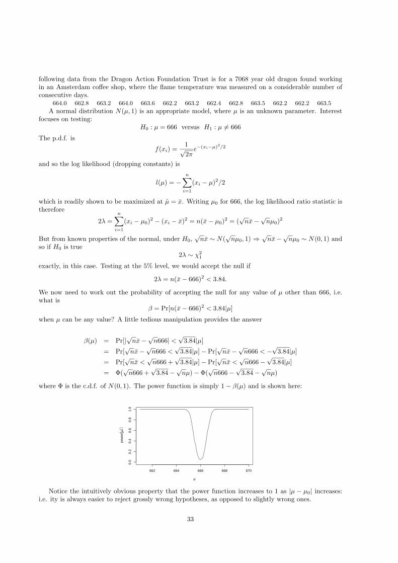
following data from the Dragon Action Foundation Trust is for a 7068 year old dragon found workingin an Amsterdam coffee shop, where the flame temperature was measured on a considerable number ofconsecutive days.

664.0 662.8 663.2 664.0 663.6 662.2 663.2 662.4 662.8 663.5 662.2 662.2 663.5

A normal distribution N(µ, 1) is an appropriate model, where µ is an unknown parameter. Interestfocuses on testing:

H0 : µ = 666 versus H1 : µ 6= 666

The p.d.f. is

f(xi) =1√2π

e−(xi−µ)2/2

and so the log likelihood (dropping constants) is

l(µ) = −n∑

i=1

(xi − µ)2/2

which is readily shown to be maximized at µ = x. Writing µ0 for 666, the log likelihood ratio statistic istherefore

2λ =n∑

i=1

(xi − µ0)2 − (xi − x)2 = n(x− µ0)2 = (√

nx−√nµ0)2

But from known properties of the normal, under H0,√

nx ∼ N(√

nµ0, 1) ⇒ √nx−√nµ0 ∼ N(0, 1) and

so if H0 is true2λ ∼ χ2

1

exactly, in this case. Testing at the 5% level, we would accept the null if

2λ = n(x− 666)2 < 3.84.

We now need to work out the probability of accepting the null for any value of µ other than 666, i.e.what is

β = Pr[n(x− 666)2 < 3.84|µ]

when µ can be any value? A little tedious manipulation provides the answer

β(µ) = Pr[|√nx−√n666| <√

3.84|µ]

= Pr[√

nx−√n666 <√

3.84|µ]− Pr[√

nx−√n666 < −√

3.84|µ]

= Pr[√

nx <√

n666 +√

3.84|µ]− Pr[√

nx <√

n666−√

3.84|µ]

= Φ(√

n666 +√

3.84−√nµ)− Φ(√

n666−√

3.84−√nµ)

where Φ is the c.d.f. of N(0, 1). The power function is simply 1− β(µ) and is shown here:

662 664 666 668 670

0.0

0.2

0.4

0.6

0.8

1.0

µ

pow

er(µ

)

Notice the intuitively obvious property that the power function increases to 1 as |µ − µ0| increases:i.e. ity is always easier to reject grossly wrong hypotheses, as opposed to slightly wrong ones.

33

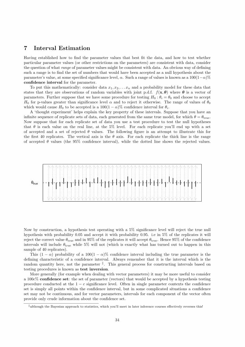
7 Interval Estimation

Having established how to find the parameter values that best fit the data, and how to test whetherparticular parameter values (or other restrictions on the parameters) are consistent with data, considerthe question of what range of parameter values might be consistent with data. An obvious way of definingsuch a range is to find the set of numbers that would have been accepted as a null hypothesis about theparameter’s value, at some specified significance level, α. Such a range of values is known as a 100(1−α)%confidence interval for the parameter.

To put this mathematically: consider data x1, x2, . . . xn and a probability model for these data thatstates that they are observations of random variables with joint p.d.f. f(x,θ) where θ is a vector ofparameters. Further suppose that we have some procedure for testing H0 : θi = θ0 and choose to acceptH0 for p-values greater than significance level α and to reject it otherwise. The range of values of θ0

which would cause H0 to be accepted is a 100(1− α)% confidence interval for θi.A ‘thought experiment’ helps explain the key property of these intervals. Suppose that you have an

infinite sequence of replicate sets of data, each generated from the same true model, for which θ = θtrue.Now suppose that for each replicate set of data you use a test procedure to test the null hypothesesthat θ is each value on the real line, at the 5% level. For each replicate you’ll end up with a setof accepted and a set of rejected θ values. The following figure is an attempt to illustrate this forthe first 40 replicates. The vertical axis is the θ axis. For each replicate the thick line is the rangeof accepted θ values (the 95% confidence interval), while the dotted line shows the rejected values.

θtrue

Now by construction, a hypothesis test operating with a 5% significance level will reject the true nullhypothesis with probability 0.05 and accept it with probability 0.95. i.e in 5% of the replicates it willreject the correct value θtrue and in 95% of the replicates it will accept θtrue. Hence 95% of the confidenceintervals will include θtrue while 5% will not (which is exactly what has turned out to happen in thissample of 40 replicates).

This (1 − α) probability of a 100(1 − α)% confidence interval including the true parameter is thedefining characteristic of a confidence interval. Always remember that it is the interval which is therandom quantity here, not the parameter ‖. This general process for constructing intervals based ontesting procedures is known as test inversion.

More generally (for example when dealing with vector parameters) it may be more useful to considera 100c% confidence set: the set of parameter (vectors) that would be accepted by a hypothesis testingprocedure conducted at the 1 − c significance level. Often in single parameter contexts the confidenceset is simply all points within the confidence interval, but in some complicated situations a confidenceset may not be continuous, and for vector parameters, intervals for each component of the vector oftenprovide only crude information about the confidence set.

‖although the Bayesian approach to statistics, which you’ll meet in later inference courses effectively reverses this!

34

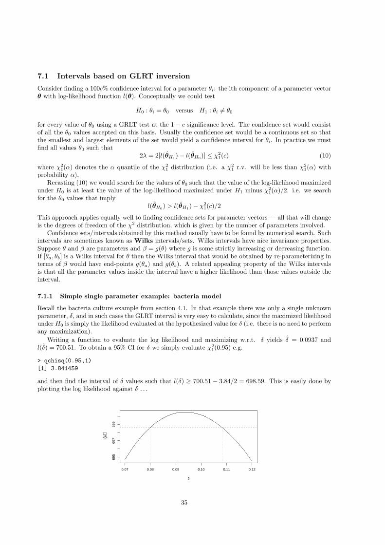
7.1 Intervals based on GLRT inversion

Consider finding a 100c% confidence interval for a parameter θi: the ith component of a parameter vectorθ with log-likelihood function l(θ). Conceptually we could test

H0 : θi = θ0 versus H1 : θi 6= θ0

for every value of θ0 using a GRLT test at the 1− c significance level. The confidence set would consistof all the θ0 values accepted on this basis. Usually the confidence set would be a continuous set so thatthe smallest and largest elements of the set would yield a confidence interval for θi. In practice we mustfind all values θ0 such that

2λ = 2[l(θH1)− l(θH0)] ≤ χ21(c) (10)

where χ21(α) denotes the α quantile of the χ2

1 distribution (i.e. a χ21 r.v. will be less than χ2

1(α) withprobability α).

Recasting (10) we would search for the values of θ0 such that the value of the log-likelihood maximizedunder H0 is at least the value of the log-likelihood maximized under H1 minus χ2

1(α)/2. i.e. we searchfor the θ0 values that imply

l(θH0) > l(θH1)− χ21(c)/2

This approach applies equally well to finding confidence sets for parameter vectors — all that will changeis the degrees of freedom of the χ2 distribution, which is given by the number of parameters involved.

Confidence sets/intervals obtained by this method usually have to be found by numerical search. Suchintervals are sometimes known as Wilks intervals/sets. Wilks intervals have nice invariance properties.Suppose θ and β are parameters and β = g(θ) where g is some strictly increasing or decreasing function.If [θa, θb] is a Wilks interval for θ then the Wilks interval that would be obtained by re-parameterizing interms of β would have end-points g(θa) and g(θb). A related appealing property of the Wilks intervalsis that all the parameter values inside the interval have a higher likelihood than those values outside theinterval.

7.1.1 Simple single parameter example: bacteria model

Recall the bacteria culture example from section 4.1. In that example there was only a single unknownparameter, δ, and in such cases the GLRT interval is very easy to calculate, since the maximized likelihoodunder H0 is simply the likelihood evaluated at the hypothesized value for δ (i.e. there is no need to performany maximization).

Writing a function to evaluate the log likelihood and maximizing w.r.t. δ yields δ = 0.0937 andl(δ) = 700.51. To obtain a 95% CI for δ we simply evaluate χ2

1(0.95) e.g.

> qchisq(0.95,1)[1] 3.841459

and then find the interval of δ values such that l(δ) ≥ 700.51 − 3.84/2 = 698.59. This is easily done byplotting the log likelihood against δ . . .

0.07 0.08 0.09 0.10 0.11 0.12

695

697

699

δ

l(δ)

35

where the continuous curve is the log-likelihood and values of δ for which the log-likelihood is above thehorizontal line form the approximate 95% confidence set. The approximate 95% confidence interval liesbetween the two dashed vertical lines and is (0.0799,0.1083) — given the function that evaluates thelikelihood it is very easy to search for these values numerically.

The m.l.e. model and the models implied by the limits of the confidence interval are overlaid on aplot of the data in the following figure.

0 5 10 15

010

2030

4050

Time (hours)

Cel

l cou

nt

7.1.2 Multi-parameter example: AIDS epidemic model

Now consider obtaining an approximate 95% confidence set for the parameters α and β of the model forAIDS in Belgium from section 4.2. In this case we need to find all the values of α0 and β0 that wouldlead to

H0 : α = α0, β = β0

being accepted when tested against an alternative of no restriction on the parameters at the 0.05 signifi-cance level. That is we need to find all the α0 and β0 values that imply that

l(α, β)− l(α0, β0) < χ22(0.95)/2

where α, β are the m.l.e.s under H1. Again it will be necessary to search for the parameter valuesnumerically. A simple approach is to evaluate the log-likelihood over a grid of α0, β0 values and thenproduce a contour plot of the log-likelihood. From the contour plot the region for which the likelihood isgreater than l(α, β)− χ2

2(0.95)/2 can be read off.In fact in S things are even simpler, since you can provide the contour routine with the levels at

which contours should be drawn and can hence request a single contour at l(α, α) − χ22(0.95)/2. The

following illustrates this (assuming that the data are already read in and the log likelihood is given by afunction ll.).

er<-optim(c(10,.1),ll,control=list(fnscale=-1),method="BFGS",y=y,t=t)boundary<-er$value-qchisq(0.95,df=2)/2 # threshold for inclusion in confidence setm<-50 # m by m grid will be produceda<-seq(15,30,length=m) # alpha values at which to evaluate llb<-seq(0.17,0.23,length=m) # beta values at which to evaluate lllog.l<-matrix(0,m,m) # matrix to hold evaluated log-likelihoodfor (i in 1:m) for (j in 1:m) log.l[i,j]<-ll(c(a[i],b[j]),y,t) # evaluate log-likcontour(a,b,log.l,levels=boundary) # produce contour plot with 1 contour at boundarypoints(er$par[1],er$par[2],pch=3) # add location of m.l.e.

The results are as follows, with the continuous curve illustrating the boundary of the confidence set forα, β, with every point within the curve lying within the set. (While the given code will run in bothS-PLUS and R, the plot was actually produced in R which has some extra labelling facilities not availablein S-PLUS.)

36

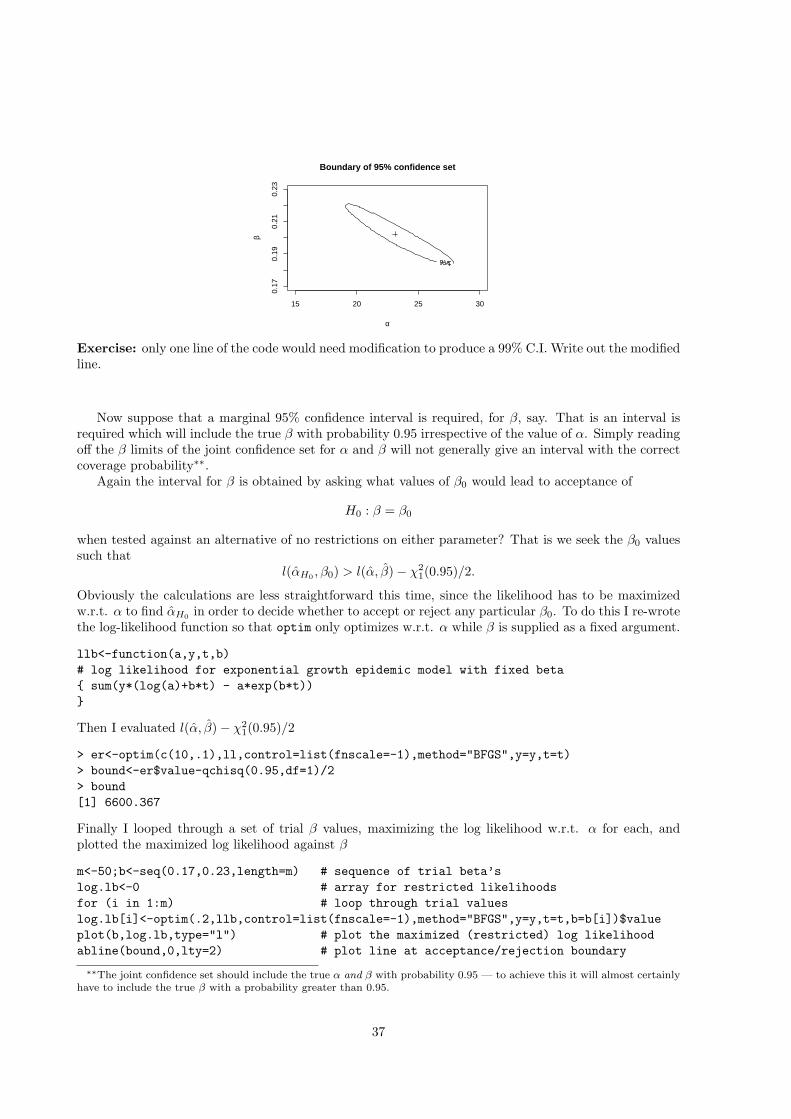
Boundary of 95% confidence set

α

β

15 20 25 30

0.17

0.19

0.21

0.23

Exercise: only one line of the code would need modification to produce a 99% C.I. Write out the modifiedline.

Now suppose that a marginal 95% confidence interval is required, for β, say. That is an interval isrequired which will include the true β with probability 0.95 irrespective of the value of α. Simply readingoff the β limits of the joint confidence set for α and β will not generally give an interval with the correctcoverage probability∗∗.

Again the interval for β is obtained by asking what values of β0 would lead to acceptance of

H0 : β = β0

when tested against an alternative of no restrictions on either parameter? That is we seek the β0 valuessuch that

l(αH0 , β0) > l(α, β)− χ21(0.95)/2.

Obviously the calculations are less straightforward this time, since the likelihood has to be maximizedw.r.t. α to find αH0 in order to decide whether to accept or reject any particular β0. To do this I re-wrotethe log-likelihood function so that optim only optimizes w.r.t. α while β is supplied as a fixed argument.

llb<-function(a,y,t,b)# log likelihood for exponential growth epidemic model with fixed beta{ sum(y*(log(a)+b*t) - a*exp(b*t))}

Then I evaluated l(α, β)− χ21(0.95)/2

> er<-optim(c(10,.1),ll,control=list(fnscale=-1),method="BFGS",y=y,t=t)> bound<-er$value-qchisq(0.95,df=1)/2> bound[1] 6600.367

Finally I looped through a set of trial β values, maximizing the log likelihood w.r.t. α for each, andplotted the maximized log likelihood against β

m<-50;b<-seq(0.17,0.23,length=m) # sequence of trial beta’slog.lb<-0 # array for restricted likelihoodsfor (i in 1:m) # loop through trial valueslog.lb[i]<-optim(.2,llb,control=list(fnscale=-1),method="BFGS",y=y,t=t,b=b[i])$valueplot(b,log.lb,type="l") # plot the maximized (restricted) log likelihoodabline(bound,0,lty=2) # plot line at acceptance/rejection boundary

∗∗The joint confidence set should include the true α and β with probability 0.95 — to achieve this it will almost certainlyhave to include the true β with a probability greater than 0.95.

37

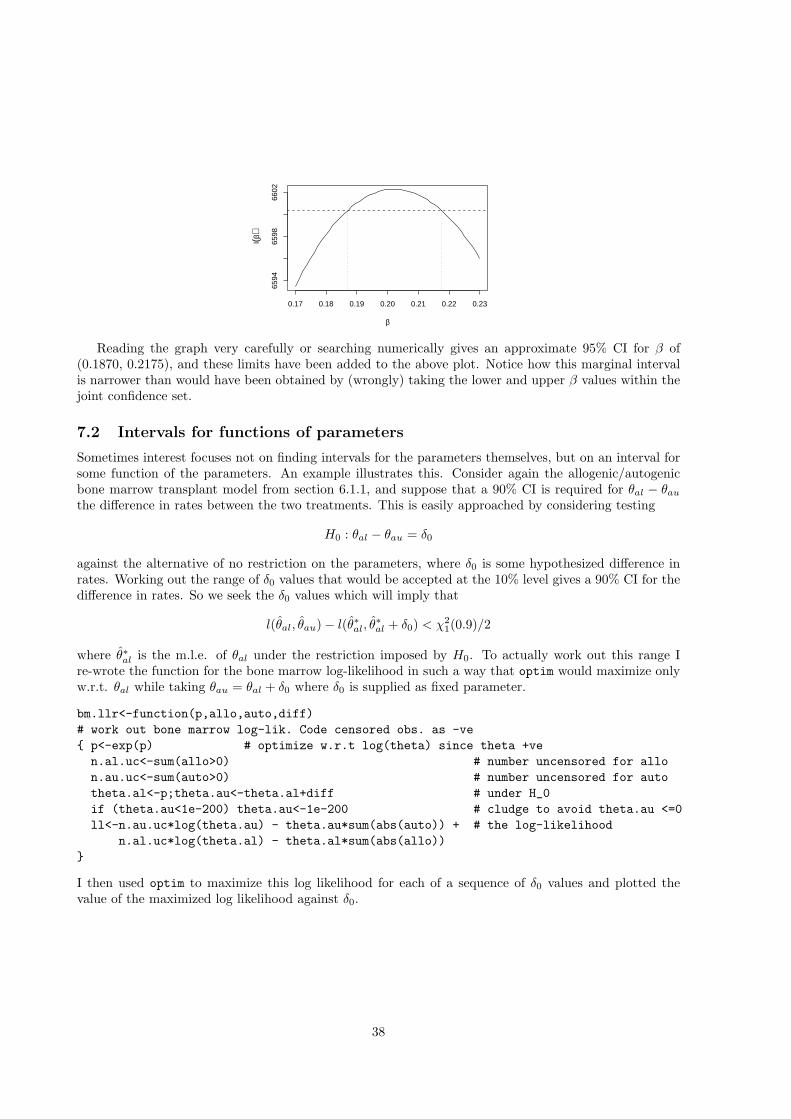
0.17 0.18 0.19 0.20 0.21 0.22 0.23

6594

6598

6602

β

l(β)

Reading the graph very carefully or searching numerically gives an approximate 95% CI for β of(0.1870, 0.2175), and these limits have been added to the above plot. Notice how this marginal intervalis narrower than would have been obtained by (wrongly) taking the lower and upper β values within thejoint confidence set.

7.2 Intervals for functions of parameters

Sometimes interest focuses not on finding intervals for the parameters themselves, but on an interval forsome function of the parameters. An example illustrates this. Consider again the allogenic/autogenicbone marrow transplant model from section 6.1.1, and suppose that a 90% CI is required for θal − θau

the difference in rates between the two treatments. This is easily approached by considering testing

H0 : θal − θau = δ0

against the alternative of no restriction on the parameters, where δ0 is some hypothesized difference inrates. Working out the range of δ0 values that would be accepted at the 10% level gives a 90% CI for thedifference in rates. So we seek the δ0 values which will imply that

l(θal, θau)− l(θ∗al, θ∗al + δ0) < χ2

1(0.9)/2

where θ∗al is the m.l.e. of θal under the restriction imposed by H0. To actually work out this range Ire-wrote the function for the bone marrow log-likelihood in such a way that optim would maximize onlyw.r.t. θal while taking θau = θal + δ0 where δ0 is supplied as fixed parameter.

bm.llr<-function(p,allo,auto,diff)# work out bone marrow log-lik. Code censored obs. as -ve{ p<-exp(p) # optimize w.r.t log(theta) since theta +ve

n.al.uc<-sum(allo>0) # number uncensored for allon.au.uc<-sum(auto>0) # number uncensored for autotheta.al<-p;theta.au<-theta.al+diff # under H_0if (theta.au<1e-200) theta.au<-1e-200 # cludge to avoid theta.au <=0ll<-n.au.uc*log(theta.au) - theta.au*sum(abs(auto)) + # the log-likelihood

n.al.uc*log(theta.al) - theta.al*sum(abs(allo))}

I then used optim to maximize this log likelihood for each of a sequence of δ0 values and plotted thevalue of the maximized log likelihood against δ0.

38

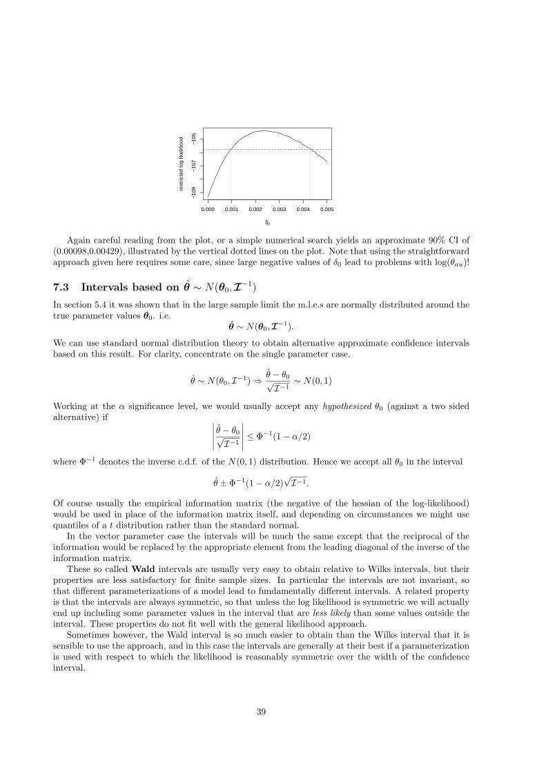
0.000 0.001 0.002 0.003 0.004 0.005

−10

9−

107

−10

5

δ0

rest

ricte

d lo

g lik

elih

ood

Again careful reading from the plot, or a simple numerical search yields an approximate 90% CI of(0.00098,0.00429), illustrated by the vertical dotted lines on the plot. Note that using the straightforwardapproach given here requires some care, since large negative values of δ0 lead to problems with log(θau)!

7.3 Intervals based on θ ∼ N(θ0, I−1)

In section 5.4 it was shown that in the large sample limit the m.l.e.s are normally distributed around thetrue parameter values θ0. i.e.

θ ∼ N(θ0, I−1).

We can use standard normal distribution theory to obtain alternative approximate confidence intervalsbased on this result. For clarity, concentrate on the single parameter case.

θ ∼ N(θ0, I−1) ⇒ θ − θ0√I−1

∼ N(0, 1)

Working at the α significance level, we would usually accept any hypothesized θ0 (against a two sidedalternative) if ∣∣∣∣∣

θ − θ0√I−1

∣∣∣∣∣ ≤ Φ−1(1− α/2)

where Φ−1 denotes the inverse c.d.f. of the N(0, 1) distribution. Hence we accept all θ0 in the interval

θ ± Φ−1(1− α/2)√I−1.

Of course usually the empirical information matrix (the negative of the hessian of the log-likelihood)would be used in place of the information matrix itself, and depending on circumstances we might usequantiles of a t distribution rather than the standard normal.

In the vector parameter case the intervals will be much the same except that the reciprocal of theinformation would be replaced by the appropriate element from the leading diagonal of the inverse of theinformation matrix.

These so called Wald intervals are usually very easy to obtain relative to Wilks intervals, but theirproperties are less satisfactory for finite sample sizes. In particular the intervals are not invariant, sothat different parameterizations of a model lead to fundamentally different intervals. A related propertyis that the intervals are always symmetric, so that unless the log likelihood is symmetric we will actuallyend up including some parameter values in the interval that are less likely than some values outside theinterval. These properties do not fit well with the general likelihood approach.

Sometimes however, the Wald interval is so much easier to obtain than the Wilks interval that it issensible to use the approach, and in this case the intervals are generally at their best if a parameterizationis used with respect to which the likelihood is reasonably symmetric over the width of the confidenceinterval.

39

7.3.1 Wald interval example: AIDS again

Consider estimating a 95% CI for the parameter β for the AIDS model example using the Wald approach.To do this requires that we evaluate the hessian matrix (second derivative matrix) of the log likelihood:optim will actually estimate this for us if specify hessian=TRUE in its argument list. Here is the S codeto evaluate the Wald interval.

> # maximize AIDS log-likelihood and hessian at the m.l.e.> m1<-optim(c(10,.1),ll,control=list(fnscale=-1),method="BFGS",hessian=TRUE,y=y,t=t)> V<-solve(-m1$hessian) # find the inverse of -H, the empirical information> b.hat<-m1$par[2] # m.l.e of beta> sigma.b<-sqrt(V[2,2]) # s.d. of estimator of beta> b.hat-1.96*sigma.b;b.hat+1.96*sigma.b # interval limits[1] 0.1868727[1] 0.2173361

The 95% CI (0.1869,0.2173) is very close to the previous Wilks estimated interval of (0.1870, 0.2175),largely because the log likelihood is almost symmetric w.r.t. β over this sort of range.

7.4 Induced confidence intervals/ confidence sets

If A is a c% confidence set for a parameter θ and g is a strictly increasing or strictly decreasing functionof θ then B = {g(θ∗) : θ∗ ∈ A} is a c% confidence set for g(θ). The proof is almost trivial. If A is one ofthe c% of sets containing the true θ then B contains the true g(θ), while if A is one of the (100 − c)%of confidence sets not containing the true θ then B will not include the true g(θ). This establishes thatB has the correct coverage probability. In the vector parameter case the same argument holds providedthat every single point in the parameter space of θ results in a unique single point in the space of g(θ).

If the strict monotonicity/unique image property of g does not hold then we can not generally constructan interval with the correct coverage probability. In this case any A containing the true θ would stillresult in a B containing the true g(θ), but now it is also possible for some A not containing the true θ toinduce a set B which does include the true g(θ). i.e. in this case B has too high a coverage probability.

For example, if [a, b] is a 99% confidence interval for θ then [log(a), log(b)] is a 95% CI for log(θ),while [1/b, 1/a] is a 99% CI for 1/θ.

8 Assumptions of the large sample results

Implicit in the derivations of the large sample properties of maximum likelihood estimation were someassumptions which it is now as well to state explicitly.

1. The parameter space is finite dimensional - i.e. θ is finite dimensional and the true θ lies in theinterior of the space, not on a boundary.

2. The probability distributions defined by any two distinct θ are distinct.

3. The first three derivatives of the log-likelihood w.r.t. θ exist in the neighbourhood of the trueparameter value (and in that neighbourhood the magnitude of the third derivative divided by thesample size is bounded above by a function of the data, whose expectation exists!)

4. Result 3 from section 5.2 holds.

The properties are generally required to justify the Taylor expansions used, for example. The assumptionsare sufficient, but not always necessary, so the results may sometimes hold even if one or more of theassumptions are violated (but in such cases they need different justification).

40