inference on treatment effects after selection amongst ... · inference on treatment effects after...
TRANSCRIPT

INFERENCE ON TREATMENT EFFECTS AFTER SELECTION AMONGST
HIGH-DIMENSIONAL CONTROLS
A. BELLONI, V. CHERNOZHUKOV, AND C. HANSEN
Abstract. We propose robust methods for inference about the effect of a treatment variable on a
scalar outcome in the presence of very many regressors in a model with possibly non-Gaussian and
heteroscedastic disturbances. We allow for the number of regressors to be larger than the sample
size. To make informative inference feasible, we require the model to be approximately sparse; that
is, we require that the effect of confounding factors can be controlled for up to a small approximation
error by including a relatively small number of variables whose identities are unknown. The latter
condition makes it possible to estimate the treatment effect by selecting approximately the right set
of regressors. We develop a novel estimation and uniformly valid inference method for the treatment
effect in this setting, called the “post-double-selection” method.
The main attractive feature of our method is that it allows for imperfect selection of the controls
and provides confidence intervals that are valid uniformly across a large class of models. In contrast,
standard post-model selection estimators fail to provide uniform inference even in simple cases with
a small, fixed number of controls. Thus, our method resolves the problem of uniform inference
after model selection for a large, interesting class of models. We also present a generalization of our
method to a fully heterogeneous model with a binary treatment variable. We illustrate the use of
the developed methods with numerical simulations and an application that considers the effect of
abortion on crime rates.
Key Words: treatment effects, partially linear model, high-dimensional-sparse regression, in-
ference under imperfect model selection, uniformly valid inference after model selection, average
treatment effects, Lasso
1. Introduction
Many empirical analyses focus on estimating the structural, causal, or treatment effect of some
variable on an outcome of interest. For example, we might be interested in estimating the causal
Date: First version: May 2010. This version is of October 17, 2013. This is a revision of a 2011 ArXiv/CEMMAP
paper entitled “Estimation of Treatment Effects with High-Dimensional Controls”.
We thank five anonymous referees, the editor of the Review, Stephane Bonhomme, the co-editor of Econometrica,
James Stock, Ted Anderson, Takeshi Amemiya, Mathias Cattaneo, Gary Chamberlain, Denis Chetverikov, Graham
Elliott, Max Farrell, Eric Tchetgen, Bruce Hansen, James Hamilton, Jin Hahn, Han Hong, Guido Imbens, Zhipeng
Liao, Tom MaCurdy, Anna Mikusheva, Whitney Newey, Alexei Onatsky, Joseph Romano, Shinich Sakata, Andres
Santos, Qi-man Shao, Mathew Shum, Chris Sims, Harrison Zhou, and participants of 10th Econometric World Con-
gress in Shanghai in 2010, Caltech, CIREQ-Montreal, Harvard-MIT, UCL, UCLA, UC San-Diego, USC, UC-Davis,
Princeton, Stanford, 2011 Infometrics Workshop, and Yale NSF 2012 conference on “High-Dimensional Statistics”
for extremely helpful comments.1

2 BELLONI CHERNOZHUKOV HANSEN
effect of some government policy on an economic outcome such as employment. Since economic
policies and many other economic variables are not randomly assigned, economists rely on a variety
of quasi-experimental approaches based on observational data when trying to estimate such effects.
One important method is based on the assumption that the variable of interest can be taken as
randomly assigned after controlling for a sufficient set of other factors; see, for example, Heckman,
LaLonde, and Smith (1999) and Imbens (2004).
A problem empirical researchers face when relying on a conditional-on-observables identification
strategy for estimating a structural effect is knowing which controls to include. Typically, economic
intuition will suggest a set of variables that might be important but will not identify exactly which
variables are important or the functional form with which variables should enter the model. This
lack of clear guidance about what variables to use leaves researchers with the problem of selecting
a set of controls from a potentially vast set of variables including raw regressors available in the
data as well as interactions and other transformations of these regressors. A typical economic study
will rely on an ad hoc sensitivity analysis in which a researcher reports results for several different
sets of controls in an attempt to show that the parameter of interest that summarizes the causal
effect of the policy variable is insensitive to changes in the set of control variables. See Donohue III
and Levitt (2001), which we use as the basis for the empirical study in this paper, or examples in
Angrist and Pischke (2008) among many other references.
We present an approach to estimating and performing inference on structural effects in an envi-
ronment where the treatment variable may be taken as exogenous conditional on observables that
complements existing strategies. We pose the problem in the framework of a partially linear model
yi = diα0 + g(zi) + ζi (1.1)
where di is the treatment/policy variable of interest, zi is a set of control variables, and ζi is an
unobservable that satisfies E[ζi | di, zi] = 0.1 The goal of the econometric analysis is to conduct
inference on the treatment effect α0. We examine the problem of selecting a set of variables
from among p potential regressors xi = P (zi), which may consist of zi and transformations of zi, to
adequately approximate g(zi) allowing for p > n. Of course, useful inference about α0 is unavailable
in this framework without imposing further structure. We impose such structure by assuming that
exogeneity of di may be taken as given once one controls linearly for a relatively small number
s < n of variables in xi whose identities are a priori unknown. This assumption implies that linear
combinations of these s unknown regressors provide approximations to g(zi) and to E[di|zi] = m(zi)
which produce relatively small approximation errors for each object. This assumption, which is
termed approximate sparsity or simply sparsity, allows us to approach the problem of estimating
α0 as a variable selection problem. This framework includes as special cases the most common
approaches to parametric and nonparametric regression analysis and allows for the realistic scenario
1We note that di does not need to be binary. This structure may also arise in the context of randomized treatment
in the case where treatment assignment depends on underlying control variables, potentially in a complicated way.
See, for example, Duflo, Glennerster, and Kremer (2008), especially Section 6.1, and Kremer and Glennerster (2011).

INFERENCE AFTER MODEL SELECTION 3
in which the researcher is unsure about exactly which variables or transformations are important
confounds and so must search among a broad set of controls.2
The main contributions of this paper are providing an estimation and inference method within a
partially linear model with potentially very high-dimensional controls and developing the supporting
theory establishing its validity uniformly across a rich class of data-generating-processes (dgps).
Our approach differs from usual post-model-selection methods that rely on a single selection step.
Rather, we use two different variable selection steps followed by a final estimation step as follows:
1. In the first step, we select a set of control variables that are useful for predicting the
treatment di. This step helps to insure validity of post-model-selection-inference by finding
control variables that are strongly related to the treatment and thus potentially important
confounding factors.
2. In the second step, we select additional variables by selecting control variables that predict
yi. This step helps to insure that we have captured important elements in the equation of
interest, ideally helping keep the residual variance small, as well as providing an additional
chance to find important confounds.
3. In the final step, we estimate the treatment effect α0 of interest by the linear regression
of yi on the treatment di and the union of the set of variables selected in the two variable
selection steps.
We provide theoretical results on the properties of the resulting treatment effect estimator and
show that it provides inference that is uniformly valid over large classes of models and also achieves
the semi-parametric efficiency bound under some conditions. Importantly, our theoretical results
allow for imperfect variable selection in either of the two variable selection steps as well as allowing
for non-Gaussianity and heteroscedasticity of the model’s errors.
We illustrate the theoretical results through an examination of the effect of abortion on crime
rates following Donohue III and Levitt (2001). In this example, we find that the formal variable
selection procedure produces a qualitatively different result than that obtained through the ad hoc
set of sensitivity results presented in the original paper. By using formal variable selection, we
select a small set of between eight and twelve variables depending on the outcome, compared to
the set of eight variables considered by Donohue III and Levitt (2001). Once this set of variables is
linearly controlled for, the estimated abortion effect is rendered imprecise. The selected variables
differ substantially from the eight variables used in Donohue III and Levitt (2001) and are generally
related to nonlinear trends that depend on initial state-level characteristics. It is interesting that
2High-dimensional xi typically occurs in either of two ways. First, the baseline set of conditioning variables itself
may be large so xi = zi, and we assume g(zi) = g(xi) ≈ x′iβg. Second, zi may be low-dimensional, but one may wish
to entertain many nonlinear transformations of zi in forming xi = P (zi) as in traditional series-based estimation of
the partially linear model. In the second case, one might prefer to refer to zi as the controls and xi as something
else, such as technical regressors. For simplicity of exposition and as the formal development in the paper is agnostic
about the source of high-dimensional xi, we call the variables in xi controls or control variables in either case.

4 BELLONI CHERNOZHUKOV HANSEN
Foote and Goetz (2008) raise a similar point based on intuitive grounds and additional data in a
comment on Donohue III and Levitt (2001). Foote and Goetz (2008) find that a linear trend inter-
acted with crime rates, computed before abortion could have had an effect, renders the estimated
abortion effects imprecise.3 Overall, finding that a formal, rigorous approach to variable selection
produces a qualitatively different result than a more ad hoc approach suggests that these meth-
ods might be used to complement economic intuition in selecting control variables for estimating
treatment effects in settings where treatment is taken as exogenous conditional on observables.
Relationship to literature. We contribute to several existing literatures. First, we contribute
to the literature on semi-parametric estimation of partially linear models; see Donald and Newey
(1994), Hardle, Liang, and Gao (2000), Robinson (1988), and others.4 We differ from most of the
existing literature which considers p n series terms by allowing p n series terms from which
we select s n terms to construct the regression fits. Considering an initial broad set of terms
allows for more refined approximations of regression functions relative to the usual approach that
uses only a few low-order terms. See, for example, Belloni, Chernozhukov, and Hansen (2011) for
a wage function example and Section 4 for theoretical examples. However, our most important
contribution is to allow for data-dependent selection of the appropriate series terms. The previous
literature on inference in the partially linear model generally takes the series terms as given without
allowing for their data-driven selection. However, selection of series terms is crucial for achieving
consistency when p n and is needed for increasing efficiency even when p = Cn with C < 1.5
Second, we contribute to the literature on the estimation of treatment effects. We note that
the policy variable di does not have to be binary in our framework. However, our method has
a useful interpretation related to the propensity score when di is binary. In the first selection
step, we select terms from xi that predict the treatment di, i.e. terms that explain the propensity
score. We also select terms from xi that predict yi, i.e. terms that explain the outcome regression
function. Then we run a final regression of yi on the treatment di and the union of selected
terms. Thus, our procedure relies on the selection of variables relevant for both the propensity
3Donohue III and Levitt (2008) provide yet more data and a more flexible specification in response to Foote and
Goetz (2008). In a supplement available at http://faculty.chicagobooth.edu/christian.hansen/research/, we provide
additional results based on Donohue III and Levitt (2008). The conclusions are similar to those obtained in this
paper in that we find the estimated abortion effect becomes imprecise once one allows for a broad set of controls and
selects among them. However, the specification of Donohue III and Levitt (2008) relies on a large number of district
cross time fixed effects and so does not immediately fit into our regularity conditions. We conjecture the methodology
continues to work in this case but leave verification to future research.4Following Robinson (1988)’s method, estimation of the parameters of the linear part of a partially linear model
is typically done by regressing yi − E[yi|zi] on di − E[di|zi] where E[yi|zi] and E[di|zi] are preliminary nonparametric
estimators of the conditional expectations of yi and di given zi under the assumption that dim(zi) is small. Our
approach implicitly fits within this framework where we are offering selection based estimators of the conditional
expectation functions.5 Cattaneo, Jansson, and Newey (2010) derive properties of series estimator under p = Cn, C < 1, asymptotics.
It follows from their results that, under homoscedasticity, the series estimator achieves the semiparametric efficiency
bound only if C → 0.

INFERENCE AFTER MODEL SELECTION 5
score and the outcome regression and is related to treatment effects estimators that use regression
adjustment after conditioning on the propensity score. Relying on selecting variables that are
important for both objects allows us to achieve two goals: we obtain uniformly valid confidence
sets for α0 despite imperfect model selection, and we achieve full efficiency for estimating α0 in the
homoscedastic case. The relation of our approach to the propensity score brings about interesting
connections to the treatment effects literature. Hahn (1998), Heckman, Ichimura, and Todd (1998),
and Abadie and Imbens (2011) have constructed efficient regression or matching-based estimates
of average treatment effects. Hahn (1998) also shows that conditioning on the propensity score
is unnecessary for efficient estimation of average treatment effects. Hirano, Imbens, and Ridder
(2003) demonstrate that one can efficiently estimate average treatment effects using estimated
propensity score weighting alone. Robins and Rotnitzky (1995) have shown that using propensity
score modeling coupled with a parametric regression model leads to efficient estimates if either the
propensity score model or the parametric regression model is correct. While our contribution is
quite distinct from these approaches, it also highlights the important robustness role played by the
propensity score model in the selection of the right control terms for the final regression.
Third, we contribute to the literature on estimation and inference with high-dimensional data
and to the uniformity literature. There has been extensive work on estimation and perfect model
selection in both low and high-dimensional contexts; see, e.g., Hansen (2005) and Belloni, Cher-
nozhukov, and Hansen (2010) for reviews focused on econometric applications. However, there
has been little work on inference after imperfect model selection. Perfect model selection relies on
extremely unrealistic assumptions, and even moderate model selection mistakes can have serious
consequences for inference as has been shown in Potscher (2009), Leeb and Potscher (2008a), and
others. In work on instrument selection for estimation of a linear instrumental variables model,
Belloni, Chernozhukov, and Hansen (2010) and Belloni, Chen, Chernozhukov, and Hansen (2012)
have shown that moderate model selection mistakes do not prevent valid inference about low-
dimensional structural parameters by exploiting the orthogonality or “immunization” property the
problem, whereby the strength of the identification of the target parameter is not affected by any
small perturbations of the “optimal” instrument.6 The partially linear regression model (1.1) does
not immediately have the same orthogonality structure, and model selection based on the out-
come regression alone produces confidence intervals with poor coverage properties. However, our
post-double selection procedure, which also selects controls that explain E[di|zi], creates the neces-
sary orthogonality by performing two separate model selection steps. Performing the two selection
steps helps reduce omitted variable bias so that it is possible to perform uniform inference after
model selection.7 In that regard, our contribution is in the spirit of and builds upon the classical
6To the best of our knowledge, Belloni, Chernozhukov, and Hansen (2010) and Belloni, Chen, Chernozhukov, and
Hansen (2012) were the first to use this immunization/orthoganility property in the p n setup. We provide a
further discussion on this property in Section 5.7Note that this claim only applies to the main parameter α0 and does not apply to the nuisance part g. Fur-
thermore, our claim of uniformity only applies to models in which both g and m are approximately sparse. See the
remarks following Theorem 1 for further discussion.

6 BELLONI CHERNOZHUKOV HANSEN
contribution by Romano (2004) on the uniform validity of t-tests for the univariate mean. It also
shares the spirit of recent contributions, among others, by Mikusheva (2007) on uniform inference
in autoregressive models, by Andrews and Cheng (2011) on uniform inference in moment condition
models that are potentially unidentified, and by Andrews, Cheng, and Guggenberger (2011) on a
generic framework for uniformity analysis.
Finally, we contribute to the broader literature on high-dimensional estimation. For variable
selection we use `1-penalized methods, though our method and theory will allow for the use of
other methods. `1-penalized methods have been proposed for model selection problems in high-
dimensional least squares problems, e.g. Lasso in Frank and Friedman (1993) and Tibshirani
(1996), in part because they are computationally efficient. Many `1-penalized methods and related
methods have been shown to have good estimation properties even when perfect variable selection
is not feasible; see, e.g., Candes and Tao (2007), Meinshausen and Yu (2009), Bickel, Ritov, and
Tsybakov (2009), Huang, Horowitz, and Wei (2010), Belloni and Chernozhukov (2013) and the
references therein. Such methods have also been shown to extend to nonparametric and non-
Gaussian cases as in Bickel, Ritov, and Tsybakov (2009) and Belloni, Chen, Chernozhukov, and
Hansen (2012). These methods produce models with a relatively small set of variables. The last
property is important in that it leaves the researcher with a set of variables that may be examined
further; in addition it corresponds to the usual approach in economics that relies on considering a
small number of controls.
Notation. We work with triangular array data ωi,nni=1, which is an observable set of the
first n elements of the infinite data stream ωi,n∞i=1 defined on the infinite product probability
space (Ω,A,Pn), where P = Pn the probability measure or data-generating process for the entire
infinite stream can change with n. We shall use Pn (possibly dependent on n) as the sets of
potential probability measures P that satisfy certain assumptions. Each ωi,n = (y′i,n, z′i,n, d
′i,n)′ is
a vector with components defined below, and these vectors are i.n.i.d. – independent across i, but
not necessarily identically distributed. Thus, all parameters that characterize the distribution of
ωi,n∞i=1 are implicitly indexed by Pn and thus by the sample size n. We shall omit the dependence
on n and on Pn from the notation where possible. We use such array asymptotics as doing so allows
consideration of approximating sequences that better capture some finite-sample phenomena and
to insure the robustness of conclusions with respect to perturbations of the data-generating process
P along various sequences. This robustness, in turn, translates into uniform validity of confidence
regions over certain regions P = ∩n>n0P of data-generating processes, where n0 > 1 is a fixed
sample size.
We use the following empirical process notation, En[f ] := En[f(ωi)] :=∑n
i=1 f(ωi)/n, and
Gn(f) :=∑n
i=1(f(ωi) − E[f(ωi)])/√n. Since we want to deal with i.n.i.d. data, we also intro-
duce the average expectation operator : E[f ] := EEn[f ] = EEn[f(ωi)] =∑n
i=1 E[f(ωi)]/n. The
l2-norm is denoted by ‖ · ‖, and the l0-norm, denoted ‖ · ‖0, is the number of non-zero components
of a vector. We use ‖ · ‖∞ to denote the maximal element of a vector. Given a vector δ ∈ Rp, and
INFERENCE AFTER MODEL SELECTION 7
a set of indices T ⊂ 1, . . . , p, we denote by δT ∈ Rp the vector in which δTj = δj if j ∈ T and
δTj = 0 if j /∈ T . We use the notation (a)+ = maxa, 0, a ∨ b = maxa, b, and a ∧ b = mina, b.We also use the notation a . b to denote a 6 cb for some constant c > 0 that does not depend
on n; and a .P b to denote a = OP (b). For an event E, we say that E wp → 1 when E occurs
with probability approaching one as n grows. We also use to denote convergence in distribution.
Given a p-vector b, we denote support(b) = j ∈ 1, ..., p : bj 6= 0.
2. Inference on Treatment and Structural Effects Conditional on Observables
2.1. Framework. We consider the partially linear model
yi = diα0 + g(zi) + ζi, E[ζi | zi, di] = 0, (2.2)
di = m(zi) + vi, E[vi | zi] = 0, (2.3)
where yi is the outcome variable, di is the policy/treatment variable whose impact α0 we would
like to infer,8 zi represents confounding factors on which we need to condition, and ζi and vi are
disturbances.
The confounding factors zi affect the policy variable via the function m(zi) and the outcome
variable via the function g(zi). Both of these functions are unknown and potentially complicated.
We use linear combinations of control terms xi = P (zi) to approximate g(zi) and m(zi), writing
(2.2) and (2.3) as
yi = diα0 + x′iβg0 + rgi︸ ︷︷ ︸g(zi)
+ζi, (2.4)
di = x′iβm0 + rmi︸ ︷︷ ︸m(zi)
+vi, (2.5)
where x′iβg0 and x′iβm0 are approximations to g(zi) and m(zi), and rgi and rmi are the corresponding
approximation errors. In order to allow for a flexible specification and incorporation of pertinent
confounding factors, the vector of controls, xi = P (zi), can have dimension p = pn which can be
large relative to the sample size. Specifically, our results require log p = o(n1/3) along with other
technical conditions. High-dimensional regressors xi = P (zi) could arise for different reasons. For
instance, the list of available controls could be large, i.e. xi = zi as in e.g. Koenker (1988). It could
also be that many technical controls are present; i.e. the list xi = P (zi) could be composed of a large
number of transformations of elementary regressors zi such as B-splines, dummies, polynomials,
and various interactions as in Newey (1997), Chen (2007), or Chen and Pouzo (2009, 2012).
Having very many controls creates a challenge for estimation and inference. A key condition that
makes it possible to perform constructive estimation and inference in such cases is termed sparsity.
Sparsity is the condition that there exist approximations x′iβg0 and x′iβm0 to g(zi) and m(zi) in
8We consider the case where di is a scalar for simplicity. Extension to the case where di is a vector of fixed, finite
dimension is accomplished by introducing an equation like (2.3) for each element of the vector.

8 BELLONI CHERNOZHUKOV HANSEN
(2.4)-(2.5) that require only a small number of non-zero coefficients to render the approximation
errors rgi and rmi small relative to estimation error. More formally, sparsity relies on two conditions.
First, there exist βg0 and βm0 such that at most s = sn n elements of βm0 and βg0 are non-zero
so that
‖βm0‖0 6 s and ‖βg0‖0 6 s.
Second, the sparsity condition requires the size of the resulting approximation errors to be small
compared to the conjectured size of the estimation error:
E[r2gi]1/2 .√s/n and E[r2mi]1/2 .
√s/n.
Note that the size of the approximating model s = sn can grow with n just as in standard series
estimation.
The high-dimensional-sparse-model framework outlined above extends the standard framework
in the treatment effect literature which assumes both that the identities of the relevant controls
are known and that the number of such controls s is much smaller than the sample size. Instead,
we assume that there are many, p, potential controls of which at most s controls suffice to achieve
a desirable approximation to the unknown functions g(·) and m(·) and allow the identity of these
controls to be unknown. Relying on this assumed sparsity, we use selection methods to select
approximately the right set of controls and then estimate the treatment effect α0.
2.2. The Method: Least Squares after Double Selection. To define the method, we first
write the reduced form corresponding to (2.2)-(2.3) as
yi = x′iβ0 + ri + ζi, (2.6)
di = x′iβm0 + rmi + vi, (2.7)
where β0 := α0βm0 +βg0, ri := α0rmi+ rgi, ζi := α0vi+ ζi. We have two equations and hence can
apply model selection methods to each equation to select control terms. Given the set of selected
controls from (2.6) and (2.7), we can estimate α0 by a least squares regression of yi on di and the
union of the selected controls. Inference on α0 may then be performed using conventional methods
for inference about parameters estimated by least squares.
The most important feature of this method is that it does not rely on the highly unrealistic as-
sumption of perfect model selection which is often invoked to justify inference after model selection.
Intuitively, this procedure works well since we are more likely to recover key controls by considering
selection of controls from both equations instead of just considering selection of controls from the
single equation (2.4) or (2.6). In finite-sample experiments, single-selection methods essentially fail,
providing poor inference relative to the double-selection method outlined above. This performance

INFERENCE AFTER MODEL SELECTION 9
is also supported theoretically by the fact that the double-selection method requires weaker regu-
larity conditions for its validity and for attaining the semi-parametric efficiency bound9 than the
single selection method.
Now we formally define the post-double-selection estimator: Let I1 denote the control terms
selected by a variable selector computed using data (yi, xi) = (di, xi), i = 1, ..., n, and let I2 denote
the control terms selected by a variable selector computed using data (yi, xi) = (yi, xi), i = 1, ..., n.
The post-double-selection estimator α of α0 is defined as the least squares estimator obtained by
regressing yi on di and the selected control terms xij with j ∈ I ⊇ I1 ∪ I2:
(α, β) = argminα∈R,β∈Rp
En[(yi − diα− x′iβ)2] : βj = 0,∀j 6∈ I. (2.8)
The set I may contain variables that were not selected in the variable selection steps with indices
in a set, say I3, that the analyst thinks are important for ensuring robustness. We call I3 the
amelioration set. Thus,
I = I1 ∪ I2 ∪ I3; (2.9)
let s = ‖I‖0 and sj = ‖Ij‖0 for j = 1, 2, 3. We define a feasible Lasso estimator below and focus
on the use of feasible Lasso for variable selection in the majority of results in this paper. When
feasible Lasso is used to construct I1 and I2, we refer to the post-double-selection estimator as the
post-double-Lasso estimator. When other model selection devices are used to construct I1 and I2,
we refer to the estimator as the generic post-double-selection estimator.
The main theoretical result of the paper shows that the post-double-selection estimator α obeys
([Ev2i ]−1E[v2i ζ
2i ][Ev2i ]
−1)−1/2√n(α− α0) N(0, 1) (2.10)
under approximate sparsity conditions, uniformly within a rich set of data generating processes.
We also show that the standard plug-in estimator for standard errors is consistent in these settings.
Figure 2.2 (right panel) illustrates the result (2.10) by showing that the finite-sample distribution
of our post-double-Lasso estimator is very close to the normal distribution. In contrast, Figure
2.2 (left panel) illustrates the problem with the traditional post-single-selection estimator based on
(2.4), showing that its distribution is bimodal and sharply deviates from the normal distribution.
2.3. Selection of controls via feasible Lasso Methods. Here we describe feasible variable
selection via Lasso. Note that each of the regression equations above is of the form
yi = x′iβ0 + ri︸ ︷︷ ︸f(zi)
+εi,
where f(zi) is the regression function, x′iβ0 is the approximation based on the dictionary xi = P (zi),
ri is the approximation error, and εi is the error. We use the version of the Lasso estimator from
9The semi-parametric efficiency bound of Robinson (1988) is attained in the homoscedastic case whenever such a
bound formally applies.

10 BELLONI CHERNOZHUKOV HANSEN
−8 −7 −6 −5 −4 −3 −2 −1 0 1 2 3 4 5 6 7 80
post-single-selection estimator
−8 −7 −6 −5 −4 −3 −2 −1 0 1 2 3 4 5 6 7 80
post-double-selection estimator
Distributions of Studentized Estimators
Figure 1. The finite-sample distributions (densities) of the standard post-single selection estima-
tor (left panel) and of our proposed post-double selection estimator (right panel). The distributions
are given for centered and studentized quantities. The results are based on 10000 replications of
Design 1 described in Section 4.2, with R2’s in equation (2.6) and (2.7) set to 0.5.
Belloni, Chen, Chernozhukov, and Hansen (2012) geared for heteroscedastic, non-Gaussian cases,
which solves
minβ∈Rp
En[(yi − x′iβ)2] +λ
n‖Ψβ‖1, (2.11)
where Ψ = diag(l1, . . . , lp) is a diagonal matrix of penalty loadings and ‖Ψβ‖1 =∑p
j=1 |ljβj |. The
penalty level λ and loadings lj ’s are set as
λ = 2 ·c√nΦ−1(1−γ/2p) and lj = lj +oP (1), lj =
√En[x2ijε
2i ], uniformly in j = 1, . . . , p, (2.12)
where c > 1 and 1 − γ is a confidence level.10 The lj ’s are ideal penalty loadings that are not
observed, and we estimate lj by lj obtained via an iteration method given in Appendix A. The
validity of using these estimates was established in Belloni, Chen, Chernozhukov, and Hansen (2012)
Lemma 11. 11
A feature of the Lasso estimator is that the non-differentiability of the penalty function at zero
induces the solution β to have components set exactly to zero, and thus the Lasso solution may be
used for model selection. In this paper, we use β as a model selection device. Specifically, we only
make use of
T = support(β),
10Practical recommendations include the choice c = 1.1 and γ close to zero, for example γ = (1/n) ∧ .05.11Other methods that provably can be used in the heteroscedastic, non-Gaussian cases in the present context is
the root-Lasso estimator (Belloni, Chernozhukov, and Wang 2011) and self-tuned Dantzig estimator (Gautier and
Tsybakov 2011).

INFERENCE AFTER MODEL SELECTION 11
the labels of the regressors with non-zero estimated coefficients. We show that the selected model
T has good approximation properties for the regression function f under approximate sparsity in
Section 3.12 In what follows, we use the term feasible Lasso to refer to a Lasso estimator β solving
(2.11)-(2.12) with c > 1 and 1− γ set such that
γ = o(1) and log(1/γ) . log(p ∨ n). (2.13)
2.4. Intuition for the Importance of Double Selection. To build intuition, we discuss the
issues surrounding post-model selection inference in the case where there is only one control. In
this simple example, we illustrate that a key defect of single-selection methods is that they fail
to control omitted variables bias, and we demonstrate how double-selection helps overcome this
problem. With one control, the model is
yi = α0di + βgxi + ζi, (2.14)
di = βmxi + vi. (2.15)
For simplicity, all errors and controls are taken as normal,(ζi
vi
)| xi ∼ N
(0,
(σ2ζ 0
0 σ2v
)), xi ∼ N(0, 1), (2.16)
where the variance of xi is normalized to be 1. The underlying probability space is equipped with
probability measure P. Let P denote the collection of all dgps P where (2.14)-(2.16) hold with
non-singular covariance matrices in (2.16). Suppose that we have an i.i.d. sample (yi, di, xi)ni=1
obeying the dgp Pn ∈ P. The subscript n signifies that the dgp and all true parameter values
may change with n to better model finite-sample phenomena such as coefficients being “close to
zero”. As in the rest of the paper, we keep the dependence of the true parameter values on n
implicit. Under the stated assumption, xi and di are jointly normal with variances σ2x = 1 and
σ2d = β2mσ2x + σ2v and correlation ρ = βmσx/σd.
The standard post-single-selection method for inference proceeds by applying a model selection
method to equation (2.14) only, followed by applying OLS to the selected model. In the model
selection stage, standard selection methods would omit xi wp → 1 if
|βg| 6`n√ncn, cn :=
σζ
σx√
1− ρ2, for some `n →∞, (2.17)
where `n is a slowly varying sequence depending only on P. On the other hand, these methods
would include xi wp → 1 if
|βg| >`′n√ncn, for some `′n > `n, (2.18)
where `′n is another slowly varying sequence in n depending only on P. As an example, one could
do model selection in the p = 1 case with a conservative t-test which drops xi if the t-statistic |t| =12In estimating the lj ’s and in Section 5, we also make use of the post-Lasso or Gauss-Lasso estimator as in
Belloni and Chernozhukov (2013) which is obtained by running conventional least squares of the outcome on just the
variables that were estimated to have non-zero coefficients by Lasso and using zero for the rest of the coefficients.
12 BELLONI CHERNOZHUKOV HANSEN
|βg|/s.e.(βg) 6 Φ−1(1−γ/2) where γ = 1/n, βg is the OLS estimator, and s.e.(βg) is the conventional
OLS standard error estimator.13 With this choice of γ, we have Φ−1(1− γ/2) =√
2 log n(1 + o(1)),
and we could then take `n =√
log n and `′n = 2√
log n. Note that Lasso selectors which we employ
in our formal analysis act much like conservative t-tests with critical value√
2 log n(1 + o(1)) in
low-dimensional settings, so our discussion here applies if Lasso selection is used in place of the
conservative t-test.
The behavior of the resulting post-single-selection estimator, α is then heavily influenced by the
sequence of underlying dgps. Under sequences of models Pn such that (2.18) holds xi is included
wp → 1. The post-single-selection estimator is then the OLS estimator including both di and xi
and follows standard large sample asymptotics under Pn:
σ−1n√n(α− α0) = σ−1n En[v2i ]
−1√nEn[viζi]︸ ︷︷ ︸=:i
+oP (1) N(0, 1)
where σ2n = σ2ζ (σ2v)−1 is the semi-parametric efficiency bound for estimating α0 under homoscedas-
ticity. When βg = o(1/√n) and ρ is bounded away from 1, xi is excluded wp → 1. In this case, βg
is small enough that failing to control for xi does not introduce large omitted variables bias, and
the estimator satisfies
σ∗−1n
√n(α− α0) = σ∗−1n En[d2i ]
−1√nEn[diζi]︸ ︷︷ ︸:=i∗
+oP (1) N(0, 1)
where σ∗2n = σ2ζ (σ2d)−1 ≤ σ2n. That is, the post-single-selection estimator may achieve a variance
smaller than the semi-parametric efficiency bound under such coefficient sequences. The potential
reduction in variance is often used to motivate single-selection procedures.
This “too good” behavior of the single-selection procedure has its price, as emphasized in Leeb
and Potscher (2008b): There are plausible sequences of dgps Pn where the post-single-selection
estimator α performs very poorly. For example, consider βg = `n√ncn, so the coefficient on the
control is “moderately close to zero”. In this case, the t-test set-up above cannot distinguish this
coefficient from 0, and the control xi is dropped wp → 1. It follows that14
|σ∗−1n
√n(α− α0)| ∞. (2.19)
This poor behavior occurs because the omitted variable bias created by dropping xi scaled by√n
diverges to infinity, namely |σ∗−1n En[d2i ]−1√nEn[dixi]βg| ∝ `n → ∞. That is, the standard post-
selection estimator is not asymptotically normal and even fails to be consistent at the rate of√n
under this sequence and many other sequences with small but non-zero βg. A similar argument
can be used to show a similar failure of single-selection based solely on (2.15).
13Such a t-test is conservative in the sense that the false rejection probability is tending to zero.14Indeed, note that σ∗−1
n
√n(α − α0) = σ∗−1
n En[d2i ]−1√nEn[diζi] + σ∗−1
n En[d2i ]−1√nEn[dixi]βg := i∗ + ii∗. The
term i∗ has standard behavior; namely i∗ N(0, 1). The term ii∗ generates omitted variable bias, and it may be
arbitrarily large since, wp → 1, |ii∗| > 12|ρ|√1−ρ2
`n ∞, if `n|ρ| ∞.

INFERENCE AFTER MODEL SELECTION 13
The post-double-selection estimator, α resolves this problem by doing variable selection via
standard t-tests or Lasso-type selectors with two equations that contain the information from (2.14)
and (2.15) and then estimating α0 by regressing yi on di and the union of the selected controls.
By doing so, xi is omitted only if its coefficient in both equations is small which greatly limits the
potential for omitted variables bias. Formally, we drop xi with positive probability only if
both |βg| <`′n√ncn and |βm| <
`′n√n
(σv/σx). (2.20)
Given this property, it follows that the post-double selection estimator satisfies
σ−1n√n(α− α0) = i+ oP (1) N(0, 1), (2.21)
under any sequence of Pn ∈ P implying we get the same approximating distribution whether or
not xi is omitted. That α follows (2.21) when xi is included is obvious as in the single-selection
case. When xi is dropped, we have
σ∗−1n
√n(α− α0) = σ∗−1n En[d2i ]
−1√nEn[diζi]︸ ︷︷ ︸=i∗
+σ∗−1n En[d2i ]−1√nEn[dixi]βg︸ ︷︷ ︸=ii
.
Term ii arises due to omitted variables bias and leads to the divergent behavior of the single-
selection estimator. However, for the double-selection-estimator, we know that (2.20) holds when
xi is omitted; so we have wp → 1
|ii| 6 2σ−1ζ σdσ−2d
√nσ2x|βmβg| 6 2
σv/σd√1− ρ2
`′n2
√n
= 2(`′n)2√n→ 0.
for sensible `′n such as `′n ∝√
log n as above. Moreover, we can show i∗ − i = oP (1) under such
sequences, so the first order asymptotics of α is the same whether xi is included or excluded.
To summarize, the post-single-selection estimator may not be root-n consistent in sensible models
which translates into bad finite-sample properties. The potential poor finite-sample performance
may be clearly seen in Monte-Carlo experiments. The estimator α is thus non-regular: its first-order
asymptotic properties depend on the model sequence Pn in a strong way. In contrast, the post-
double selection estimator α guards against omitted variables bias which reduces the dependence
of the first-order behavior on Pn. This good behavior under sequences Pn translates into uniform
with respect to P ∈ P asymptotic normality.
We should note that the post-double-selection estimator is first-order equivalent to the regres-
sion including all the controls when p is small relative to n.15 This equivalence disappears under
approximating sequences with number of controls proportional to the sample size, p ∝ n, or greater
than the sample size, p n. It is these scenarios that motivate the use of selection as a means
of regularization. In these more complicated settings the intuition from this simple p = 1 example
carries through, and the post-single selection method has a highly non-regular behavior while the
post-double selection method continues to be regular.
15This equivalence may be a reason double-selection was previously overlooked, though there are higher-order
differences between the estimator using all controls and our estimator in the case where p is small relative to n.

14 BELLONI CHERNOZHUKOV HANSEN
3. Theory of Estimation and Inference
3.1. Regularity Conditions. In this section, we provide regularity conditions that are sufficient
for validity of the main estimation and inference result. We begin by stating our main condi-
tion, which contains the previously defined approximate sparsity assumption as well as other more
technical assumptions. Throughout the paper, we let c, C, and q be absolute constants, and let
`n ∞, δn 0, and ∆n 0 be sequences of absolute positive constants. By absolute constants,
we mean constants that are given, and do not depend on the dgp P = Pn.
We assume that for each n the following condition holds on dgp P = Pn.
Condition ASTE (P): Approximate Sparse Treatment Effects. (i) We observe ωi =
(yi, di, zi), i = 1, ..., n, where ωi∞i=1 are i.n.i.d. vectors on the probability space (Ω,F ,P) that obey
the model (2.2)-(2.3), and the vector xi = P (zi) is a p-dimensional dictionary of transformations
of zi, which may depend on n but not on P. (ii) The true parameter value α0, which may depend
on P, is bounded, |α0| 6 C. (iii) Functions m and g admit an approximately sparse form. Namely
there exists s > 1 and βm0 and βg0, which depend on n and P, such that
m(zi) = x′iβm0 + rmi, ‖βm0‖0 6 s, E[r2mi]1/2 6 C√s/n, (3.22)
g(zi) = x′iβg0 + rgi, ‖βg0‖0 6 s, E[r2gi]1/2 6 C√s/n. (3.23)
(iv) The sparsity index obeys s2 log2(p ∨ n)/n 6 δn and the size of the amelioration set obeys
s3 6 C(1 ∨ s1 ∨ s2). (v) For vi = vi + rmi and ζi = ζi + rgi we have |E[v2i ζ2i ]− E[v2i ζ
2i ]| 6 δn, and
E[|vi|q + |ζi|q] 6 C for some q > 4. Moreover, maxi6n ‖xi‖2∞sn−1/2+2/q 6 δn wp 1−∆n.
Comment 3.1. The approximate sparsity (iii) and rate condition (iv) are the main conditions for
establishing the key inferential result. We present a number of primitive examples to show that
these conditions contain standard models used in empirical research as well as more flexible models.
Condition (iv) requires that the size s3 of the amelioration set I3 should not be substantially larger
than the size of the set of variables selected by the Lasso method. Simply put, if we decide to
include controls in addition to those selected by Lasso, the total number of additions should not
dominate the number of controls selected by Lasso. This and other conditions will ensure that the
total number s of controls obeys s .P s. We also require that s2 log2(p ∨ n)/n → 0. Note that
s is the bound on the number of regressors used by a sparse model to achieve an approximation
error of order√s/n and that the rate of convergence for the estimated coefficients would be
√s/n
if we knew the identities of these s variables. Thus, the estimated function converges to the
population function at a rate of√s/n in the idealized setting where we know the identities of the
relevant variables, and we would achieve an approximation rate of o(n−1/4) under the condition
that s2/n→ 0 in this case. When the identities of the relevant variables are unknown, we use the
stronger rate condition s2 log2(p ∨ n)/n → 0 where the additional logarithmic term is the cost of
not knowing the correct set of variables. This decrease in the rate of convergence can be substantial
for large p, for example if log p ∝ nγ for some positive γ < 1/2. This condition can be relaxed
using sample-splitting, which is done in a supplementary appendix. Condition (v) is simply a set

INFERENCE AFTER MODEL SELECTION 15
of sufficient conditions for consistent estimation of the variance of the double selection estimator.
If the regressors are uniformly bounded and the approximation errors are going to zero a.s., it is
implied by other conditions stated below; and it can also be demonstrated under other sorts of
more primitive conditions.
The next condition concerns the behavior of the Gram matrix En[xix′i]. Whenever p > n,
the empirical Gram matrix En[xix′i] does not have full rank and in principle is not well-behaved.
However, we only need good behavior of smaller submatrices. Define the minimal and maximal
m-sparse eigenvalue of a semi-definite matrix M as
φmin(m)[M ] := min16‖δ‖06m
δ′Mδ
‖δ‖2and φmax(m)[M ] := max
16‖δ‖06m
δ′Mδ
‖δ‖2. (3.24)
To assume that φmin(m)[En[xix′i]] > 0 requires that all empirical Gram submatrices formed by any
m components of xi are positive definite. We shall employ the following condition as a sufficient
condition for our results.
Condition SE (P): Sparse Eigenvalues. There is an absolute sequence `n → ∞ such that
with a high probability the maximal and minimal `ns-sparse eigenvalues are bounded from above
and away from zero. Namely with probability at least 1−∆n,
κ′ 6 φmin(`ns)[En[xix′i]] 6 φmax(`ns)[En[xix
′i]] 6 κ
′′,
where 0 < κ′ < κ′′ <∞ are absolute constants.
Comment 3.2. It is well-known that Condition SE is quite plausible for many designs of interest.
For instance, Condition SE holds if
(a) (xi)ni=1 are i.i.d. zero-mean sub-Gaussian random vectors that have population Gram matrix
E[xix′i] with minimal and maximal s log n-sparse eigenvalues bounded away from zero and
from above by absolute constants where s(log n)(log p)/n 6 δn → 0;
(b) (xi)ni=1 are i.i.d. bounded zero-mean random vectors with ‖xi‖∞ 6 Kn a.s. such that
E[xix′i] has minimal and maximal s log n-sparse eigenvalues bounded from above and away
from zero by absolute constants, where K2ns(log3 n)log(p ∨ n)/n 6 δn → 0.
The claim (a) holds by Theorem 3.2 in Rudelson and Zhou (2011)16 and claim (b) holds by Theorem
1.8 in Rudelson and Zhou (2011). Recall that a standard assumption in econometric research is to
assume that the population Gram matrix E[xix′i] has eigenvalues bounded from above and away
from zero, see e.g. Newey (1997). The conditions above allow for this and more general behavior,
requiring only that the s log n sparse eigenvalues of the population Gram matrix E[xix′i] are bounded
from below and from above.
The next condition imposes moment conditions on the structural errors and regressors.
16See also Zhou (2009) and Baraniuk, Davenport, DeVore, and Wakin (2008).

16 BELLONI CHERNOZHUKOV HANSEN
Condition SM (P): Structural Moments. There are absolute constants 0 < c < C < ∞and 4 < q <∞ such that for (yi, εi) = (yi, ζi) and (yi, εi) = (di, vi) the following conditions hold:
(i) E[|di|q] 6 C, c 6 E[ζ2i | xi, vi] 6 C and c 6 E[v2i | xi] 6 C a.s. 1 6 i 6 n,
(ii) E[|εi|q] + E[y2i ] + max16j6p
E[x2ij y2i ] + E[|x3ijε3i |] + 1/E[x2ij ] 6 C,
(iii) log3 p/n 6 δn,
(iv) max16j6p
|(En − E)[x2ijε2i ]|+ |(En − E)[x2ij y
2i ]|+ max
16i6n‖xi‖2∞
s log(n ∨ p)n
6 δn wp 1−∆n.
These conditions ensure good model selection performance of feasible Lasso applied to equations
(2.6) and (2.7). These conditions also allow us to invoke moderate deviation theorems for self-
normalized sums from Jing, Shao, and Wang (2003) to bound some important error components.
3.2. The Main Result. The following is the main result of this paper. It shows that the post-
double selection estimator is root-n consistent and asymptotically normal. Under homoscedasticity
this estimator achieves the semi-parametric efficiency bound. The result also verifies that plug-in
estimates of the standard errors are consistent.
Theorem 1 (Estimation and Inference on Treatment Effects). Let Pn be a sequence of data-
generating processes. Assume conditions ASTE (P), SM (P), and SE (P) hold for P = Pn for each
n. Then, the post-double-Lasso estimator α, constructed in the previous section, obeys as n→∞
σ−1n√n(α− α0) N(0, 1),
where σ2n = [Ev2i ]−1E[v2i ζ
2i ][Ev2i ]
−1. Moreover, the result continues to apply if σ2n is replaced by
σ2n = [Env2i ]−1En[v2i ζ2i ][Env2i ]−1, for ζi := [yi − diα − x′iβ]n/(n − s − 1)1/2 and vi := di − x′iβ,
i = 1, . . . , n where β ∈ arg minβEn[(di − x′iβ)2] : βj = 0, ∀j /∈ I where I is defined in (2.9).
Comment 3.3. (Achieving the semi-parametric efficiency bound). Note that under i.i.d.
sampling under P and conditional homoscedasticity, namely E[ζ2i |zi] = E[ζ2i ], the asymptotic vari-
ance σ2n reduces to E[v2i ]−1E[ζ2i ], which is the semi-parametric efficiency bound for the partially
linear model of Robinson (1988).
Corollary 1 (Uniformly Valid Confidence Intervals). Let Pn be the collection of all data-
generating processes P for which conditions ASTE(P), SM (P), and SE (P) hold for given n, and
let P = ∩n>n0Pn be the collection of data-generating processes for which the conditions above hold
for all n > n0. Let c(1 − ξ) = Φ−1(1 − ξ/2). The confidence regions based upon (α, σn) are valid
uniformly in P ∈ P:
limn→∞
supP∈P|P(α0 ∈ [α± c(1− ξ)σn/
√n])− (1− ξ)| = 0.
By exploiting both equations (2.4) and (2.5) for model selection, the post-double-selection
method creates the necessary adaptivity that makes it robust to imperfect model selection. Ro-
bustness of the post-double selection method is reflected in the fact that Theorem 1 permits the

INFERENCE AFTER MODEL SELECTION 17
data-generating process to change with n. Thus, the conclusions of the theorem are valid for a wide
variety of sequences of data-generating processes which in turn define the regions P of uniform va-
lidity of the resulting confidence sets. In contrast, the standard post-selection method based on
(2.4) produces confidence intervals that do not have close to correct coverage in many cases.
Comment 3.4. Our approach to uniformity analysis is most similar to that of Romano (2004),
Theorem 4. It proceeds under triangular array asymptotics, with the sequence of dgps obeying
certain constraints; then these results imply uniformity over sets of dgps that obey the constraints
for all sample sizes. This approach is also similar to the classical central limit theorems for sample
means under triangular arrays, and does not require the dgps to be parametrically (or otherwise
tightly) specified, which then translates into uniformity of confidence regions. This approach is
somewhat different in spirit to the generic uniformity analysis suggested by Andrews, Cheng, and
Guggenberger (2011).
Comment 3.5 (Limits of uniformity). Uniformity for inference about α0 holds over a large class of
approximately sparse models: models where both g(·) and m(·) are well-approximated by s n1/2
terms so that they are both estimable at o(n−1/4) rates. Approximate sparsity is more general
than assumptions often used to justify series estimation of partially linear models, so the uniformity
regions - the sets of models over which inference is valid - are substantial in that regard. We formally
demonstrate this through a series of examples in Section 4.1. Of course, for every interesting class
of models and any non-trivial inference method, one could find an even bigger class of models where
the uniformity does not apply. For example, our approach will not work in “dense” models, models
where g(·) or m(·) is not well-approximated unless s n1/2 terms are used; such dense models
would generally involve many small coefficients that decay to zero very slowly or not at all. In the
series case, such a model corresponds to a deviation from smoothness towards highly non-smooth
functions, for example functions generated as realized paths of a white noise process. The fact that
our results do not cover such models motivates further research work on inference procedures that
would provide valid inference when one considers deviations from the given class of models that are
deemed important. In the simulations in Section 4.2, we consider incorporating the ridge fit along
the other controls to be selected over using Lasso to build extra robustness against such deviations
away from approximately sparse models.
3.3. Inference after Double Selection by a Generic Selection Method. The conditions
provided so far offer a set of sufficient conditions that are tied to the use of Lasso as the model
selector. The purpose of this section is to prove that the main results apply to any other model
selection method that is able to select a sparse model with good approximation properties. As in
the case of Lasso, we allow for imperfect model selection. Next we state a high-level condition that
summarizes a sufficient condition on the performance of a model selection method that allows the
post-double selection estimator to attain good inferential properties.
Condition HLMS (P): High-Dimensional Linear Model Selection. A model selector
provides possibly data-dependent sets I1 ∪ I2 ⊆ I ⊂ 1, ..., p of covariate names such that, with

18 BELLONI CHERNOZHUKOV HANSEN
probability 1−∆n, |I| 6 Cs and
minβ:βj=0,j 6∈I1
√En[(m(zi)− x′iβ)2] 6 δnn
−1/4 and minβ:βj=0,j 6∈I2
√En[(g(zi)− x′iβ)2] 6 δnn
−1/4.
Condition HLMS requires that with high probability the selected models are sparse and gener-
ate good approximations for the functions g and m. Examples of methods producing such mod-
els include the Dantzig selector (Candes and Tao 2007), feasible Dantzig selector (Gautier and
Tsybakov 2011), Bridge estimator (Huang, Horowitz, and Ma 2008), SCAD penalized least squares
(Fan and Li 2001), square-root-Lasso (Belloni, Chernozhukov, and Wang 2011), and thresholded
Lasso (Belloni and Chernozhukov 2013), to name a few. We emphasize that, similarly to the pre-
vious arguments, these conditions allow for imperfect model selection. Nonetheless we note that
Condition HLMS implicitly assumes that tuning parameters of the model selection procedure are
set properly to achieve these conditions.
The following result establishes the inferential properties of a generic post-double-selection esti-
mator.
Theorem 2 (Estimation and Inference on Treatment Effects under High-Level Model Selection).
Let Pn be the collection of all data-generating processes P for which conditions ASTE(P), SM (P),
SE (P), and HLMS (P) hold for given n. (1) Then under any sequence Pn ∈ Pn, the generic
post-double-selection estimator α based on I, as defined in (2.8), obeys
σ−1n√n(α− α0) N(0, 1),
where σ2n = [Ev2i ]−1E[v2i ζ
2i ][Ev2i ]
−1. Moreover, the result continues to apply if σ2n is replaced by
σ2n = [Env2i ]−1En[v2i ζ2i ][Env2i ]−1, for ζi := [yi − diα − x′iβ]n/(n − s − 1)1/2 and vi := di − x′iβ,
i = 1, . . . , n where β ∈ arg minβEn[(di − x′iβ)2] : βj = 0,∀j /∈ I. (2) Moreover, let P = ∩n>n0Pn
be the collection of data-generating processes for which the conditions above hold for all n > n0.
The confidence regions based upon (α, σn) are valid uniformly in P ∈ P:
limn→∞
supP∈P|P(α0 ∈ [α± Φ−1(1− ξ/2)σn/
√n])− (1− ξ)| = 0.
4. Theoretical and Monte-Carlo Examples
4.1. Theoretical Examples. The purpose of this section is to give examples that highlight the
range of the applicability of the proposed method. In these examples, we specify primitive condi-
tions which cover certain nonparametric models and high-dimensional parametric models as corol-
laries. A supplementary appendix provides proofs for these corollaries. We emphasize that our
main regularity conditions cover even more general models which combine various features of these
examples. In all examples, the model is the partially linear model (2.2)-(2.3) of Section 2, however,
the structure for g and m will vary across examples, and so will the assumptions on the error terms
ζi and vi.

INFERENCE AFTER MODEL SELECTION 19
4.1.1. Parametric model with fixed p. We start out with a simple example, in which the dimension p
of the regressors is fixed. In practical terms this example approximates cases with p small compared
to n. This simple example is important since standard post-single-selection methods fail even in
this simple case. Specifically, they produce confidence intervals that are not valid uniformly in
the underlying data-generating process; see Leeb and Potscher (2008a). In contrast, the post-
double-selection method produces confidence intervals that are valid uniformly in the underlying
data-generating process.
Example 1. (Parametric Model with Fixed p.) Consider (Ω,A,P) as the probability space, on
which we have (yi, zi, di)∞i=1 as i.i.d. vectors obeying the model (2.2)-(2.3) with
g(zi) =
p∑j=1
βg0jzij , m(zi) =
p∑j=1
βm0jzij . (4.25)
For estimation we use xi = (zij , j = 1, ..., p)′. We assume that there are absolute constants 0 < b <
B <∞, qx > q > 4, with 4/qx + 4/q < 1, such that
b 6 E[ζ2i | xi, vi], E[|ζqi | | xi, vi] 6 B, b 6 E[v2i | xi], E[|vqi | | xi] 6 B. (4.26)
Corollary 2 (Parametric Example with Fixed p). Let P be the collection of all regression models
P that obey the conditions set forth in Example 1 for all n for the given constants (p, b, B, qx, q).
Then, any P ∈ P obeys Conditions ASTE (P) with s = p, SE (P), and SM (P) for all n > n0,
with the constants n0 and (κ′, κ′′, c, C) and sequences ∆n and δn in those conditions depending only
on (p, b, B, qx, q). Therefore, the conclusions of Theorem 1 hold for any sequence Pn ∈ P, and the
conclusions of Corollary 1 on the uniform validity of confidence intervals apply uniformly in P ∈ P.
4.1.2. Nonparametric Examples. The next examples are more substantial and include infinite-
dimensional models which we approximate with linear functional forms with potentially very many
regressors, p n. The key to estimation in these models is a smoothness condition which requires
regression coefficients to decay at some rates. In series estimation, this condition is often directly
connected to smoothness of the regression function.
Let a and A be positive constants. We shall say that a sequence of coefficients
θ = θj , j = 1, 2, ...
is a-smooth with constant A if
|θj | 6 Aj−a, j = 1, 2, ...,
which will be denoted as θ ∈ SaA. We shall say that a sequence of coefficients θ = θj , j = 1, 2, ...is a-smooth with constant A after p-rearrangement if
|θ(j)| 6 Aj−a, j = 1, 2, ..., p, |θj | 6 Aj−a, j = p+ 1, p+ 2, ...,
which will be denoted as θ ∈ SaA(p), where |θ(j)|, j = 1, ..., p denotes the decreasing rearrangement
of the numbers |θj |, j = 1, ..., p. Since SaA ⊂ SaA(p), the second kind of smoothness is strictly more
general than the first kind.
20 BELLONI CHERNOZHUKOV HANSEN
Here we use the term “smoothness” motivated by Fourier series analysis where smoothness of
functions often translates into smoothness of the Fourier coefficients in the sense that is stated
above; see, e.g., Kerkyacharian and Picard (1992). For example, if a function h : [0, 1]d 7→ Rpossesses r > 0 continuous derivatives uniformly bounded by a constant M and the terms Pj are
compactly supported Daubechies wavelets, then h can be represented as h(z) =∑∞
j=1 Pj(z)θhj ,
with |θhj | 6 Aj−r/d−1/2 for some constant A; see Kerkyacharian and Picard (1992). We also
note that the second kind of smoothness is considerably more general than the first since it allows
relatively large coefficients to appear anywhere in the series of the first p coefficients. In contrast,
the first kind of smoothness only allows relatively large coefficients among the early terms in the
series. Lasso-type methods are specifically designed to deal with the generalized smoothness of
the second kind and perform equally well under both kinds of smoothness. In the context of
series applications, smoothness of the second kind allows one to approximate functions that exhibit
oscillatory phenomena or spikes, which are associated with “high-order” series terms. An example
of this is the wage function example given in Belloni, Chernozhukov, and Hansen (2011).
Before we proceed to other examples we discuss a way to generate sparse approximations in
infinite-dimensional examples. Consider, for example, a function h that can be represented as
h(zi) =∑∞
j=1 θhjPj(zi) with coefficients θh ∈ SaA(p). In this case we can construct sparse approxi-
mations by simply thresholding to zero all coefficients smaller than 1/√n and with indices j > p.
This generates a sparsity index s 6 A1an
12a . The non-zero coefficients could be further reoptimized
by using the least squares projection. More formally, given a sparsity index s > 0, a target function
h(zi), and terms xi = (Pj(zi) : j = 1, . . . , p)′ ∈ Rp, we let
βh0 := arg min‖β‖06s
E[(h(zi)− x′iβ)2], (4.27)
and define x′iβh0 as the best s-sparse approximation to h(zi).
Example 2. (Gaussian Model with Very Large p.) Consider (Ω,A,P) as the probability space
on which we have (yi, zi, di)∞i=1 as i.i.d. vectors obeying the model (2.2)-(2.3) with
g(zi) =∞∑j=1
θgjzij , m(zi) =∞∑j=1
θmjzij . (4.28)
Assume that the infinite dimensional vector wi = (ζi, vi, z′i)′ with jth element denoted wi(j) is
jointly Gaussian with covariance operator [Cov(wi(j), wi(k))]j,k≥1 that has minimal and maximal
eigenvalues bounded below by an absolute constant κ > 0 and above by an absolute constant
κ <∞.
The main assumption that guarantees approximate sparsity is the smoothness condition on the
coefficients. Let a > 1 and 0 < A < ∞ be absolute constants. We require that the coefficients of
the expansions in (4.28) are a-smooth with constant A after p-rearrangement, namely
θm = (θmj , j = 1, 2, ...) ∈ SaA(p), θg = (θgj , j = 1, 2, ...) ∈ SaA(p).
INFERENCE AFTER MODEL SELECTION 21
For estimation purposes we shall use xi = (zij , j = 1, ..., p)′, and assume that |α0| 6 B and p = pn
obeys
n1−aa
+χ log2(p ∨ n) 6 δn, A1/an12a 6 pδn, and log3 p/n 6 δn,
for some sequence of positive constants δn 0 and absolute constants B and χ > 0.
Corollary 3 (Gaussian Nonparametric Model). Let Pn be the collection of all dgp P that obey the
conditions set forth in Example 2 for a given n and for the given constants (κ, κ, a,A,B, χ) and
sequences p = pn and δn. Then, as established in a supplementary appendix, any P ∈ Pn obeys
Conditions ASTE (P) with s = A1/an12a , SE (P), and SM (P) for all n > n0, with constants n0 and
(κ′, κ′′, c, C) and sequences ∆n and δn in those conditions depending only on (κ, κ, a, A,B, χ), p, and
δn. Therefore, the conclusions of Theorem 1 hold for any sequence Pn ∈ Pn, and the conclusions of
Corollary 1 on the uniform validity of confidence intervals apply uniformly in P ∈ P = ∩n>n0Pn.
Example 3. (Series Model with Very Large p.) Consider (Ω,A,P) as the probability space, on
which we have (yi, zi, di)∞i=1 as i.i.d. vectors obeying the model (2.2)-(2.3), with
g(zi) =
∞∑j=1
θgjPj(zi), m(zi) =
∞∑j=1
θmjPj(zi), (4.29)
where zi has support [0, 1]d with density bounded from below by constant f > 0 and above by
constant f , and Pj , j = 1, 2, ... is an orthonormal basis on L2[0, 1]d with bounded elements, i.e.
maxz∈[0,1]d |Pj(z)| 6 B for all j = 1, 2, .... Here all constants are taken to be absolute. Examples of
such orthonormal bases include canonical trigonometric bases, e.g. 1,√
2 cos(2πjz),√
2 sin(2πjz) :
j > 1 where z ∈ [0, 1].
Let a > 1 and 0 < A < ∞ be absolute constants. We require that the coefficients of the
expansions in (4.29) are a-smooth with constant A after p-rearrangement, namely
θm = (θmj , j = 1, 2, ...) ∈ SaA(p), θg = (θgj , j = 1, 2, ...) ∈ SaA(p).
For estimation purposes we shall use xi = (Pj(zi), j = 1, ..., p)′, and assume that p = pn obeys
n(1−a)/a log2(p ∨ n) 6 δn, A1/an12a 6 pδn and log3 p/n 6 δn,
for some sequence of absolute constants δn 0. We assume that there are some absolute constants
b > 0, B <∞, q > 4, with (1− a)/a+ 4/q < 0, such that
|α0| 6 B, b 6 E[ζ2i | xi, vi], E[|ζqi | | xi, vi] 6 B, b 6 E[v2i | xi], E[|vqi | | xi] 6 B. (4.30)
Corollary 4 (Nonparametric Model with Sieve-type Regressors). Let Pn be the collection of all
regression models P that obey the conditions set forth above for a given n. Then any P ∈ Pn obeys
Conditions ASTE (P) with s = A1/an12a , SE (P), and SM (P) for all n > n0, with absolute constants
in those conditions depending only on (f, f , a, A, b,B, q) and δn. Therefore, the conclusions of
Theorem 1 hold for any sequence Pn ∈ Pn, and the conclusions of Corollary 1 on the uniform
validity of confidence intervals apply uniformly in P ∈ P = ∩n>n0Pn.

22 BELLONI CHERNOZHUKOV HANSEN
4.2. Monte-Carlo Examples. In this section, we examine the finite-sample properties of the post-
double-selection method and compare its performance to that of a standard post-single-selection
method.
All of the simulation results are based on the model
yi = d′iα0 + x′iθg + σy(di, xi)ζi (4.31)
di = x′iθm + σd(xi)vi (4.32)
where (ζi, vi)′ ∼ N(0, I2) with I2 the 2× 2 identity matrix, p = dim(xi) = 200, the covariates xi ∼
N(0,Σ) with Σkj = (0.5)|j−k|, α0 = .5, and the sample size n is set to 100. Inference results for all
designs are based on conventional t-tests with standard errors calculated using the heteroscedasticity
consistent jackknife variance estimator discussed in MacKinnon and White (1985).
We report results from three different dgp’s. In the first two dgp’s, we set θg,j = cyβ0,j and
θm,j = cdβ0,j with β0,j = (1/j)2 for j = 1, ..., 200. The first dgp, which we label “Design 1,”
uses homoscedastic innovations with σy(di, xi) = σd(xi) = 1. The second dgp, “Design 2,” is
heteroscedastic with σd(xi) =
√(1+x′iβ0)
2
En(1+x′iβ0)2and σy(di, xi) =
√(1+α0di+x′iβ0)
2
En(1+α0di+x′iβ0)2 . The constants cy
and cd are chosen to generate desired population values for the reduced form R2’s, i.e. the R2’s
for equations (2.6) and (2.7). For each equation, we choose cy and cd to generate R2 = 0, .2, .4, .6,
and .8. In the heteroscedastic design, we choose cy and cd based on R2 as if (4.31) and (4.32)
held with vi and ζi homoscedastic and label the results by R2 as in Design 1. In the third design
(“Design 3”), we use a combination of deterministic and random coefficients. For the deterministic
coefficients, we set θg,j = cy(1/j)2 for j ≤ 5 and θm,j = cd(1/j)
2 for j ≤ 5. We then generate
the remaining coefficients as iid draws from (θg,j , θm,j)′ ∼ N(02×1, (1/p)I2). For each equation, we
choose cy and cd to generate R2 = 0, .2, .4, .6, and .8 in the case that all of the random coefficients
are exactly equal to 0 and label the results by R2 as in Design 1. We draw new x’s, ζ’s, and v’s at
every simulation replication, and we also generate new θ’s at every simulation replication in Design
3.
We consider Designs 1 and 2 to be baseline designs. These designs do not have exact sparse
representations but have coefficients that decay quickly so that approximately sparse representations
are available. Design 3 is meant to introduce a modest deviation from the approximately sparse
model towards a model with many small, uncorrelated coefficients. Using this we shall document
that our proposed procedure still performs reasonably well, although it could be improved by
incorporation of a ridge fit as one of regressors over which selection occurs.17
17In a supplementary appendix, we present results for 26 additional designs. The results presented in this section
are sufficient to illustrate the general patterns from the larger set of results. In particular, the post-double-Lasso
performed very well across all simulation designs where approximate sparsity provides a reasonable description of
the dgp. Unsurprisingly, the performance deteriorates as one deviates from the smooth/approximately sparse case.
However, the post-double-Lasso outperformed all other feasible procedures considered in all designs.

INFERENCE AFTER MODEL SELECTION 23
We report results for five different procedures. Two of the procedures are infeasible benchmarks:
Oracle and Double-Selection Oracle estimators, which use knowledge of the true coefficient struc-
tures θg and θm and are thus unavailable in practice. The Oracle estimates α by running ordinary
least squares of yi − x′iθg on di, and the Double-Selection Oracle estimates α by running ordinary
least squares of yi−x′iθg on di−x′iθm. The other procedures we consider are feasible. One procedure
is the standard post-single selection estimator – the Post-Lasso – which applies Lasso to equation
(4.31) without penalizing α, the coefficient on di, to select additional control variables from among
x. Estimates of α0 are then obtained by OLS regression of yi on di and the set of additional
controls selected in the Lasso step and inference using the Post-Lasso estimator proceeds using
conventional heteroscedasticity robust OLS inference from this regression. Post-Double-Selection
or Post-Double-Lasso is the feasible procedure advocated in this paper. We run Lasso of yi on xi to
select a set of predictors for yi and run Lasso of di on xi to select a set of predictors for di. α0 is then
estimated by running OLS regression of yi on di and the union of the sets of regressors selected in
the two Lasso runs, and inference is simply the usual heteroscedasticity robust OLS inference from
this regression.18 Post-Double-Selection + Ridge is an ad hoc variant of Post-Double-Selection in
which we add the ridge fit from equation (4.32) as an additional potential regressor that may be
selected by Lasso. The ridge fit for di is x′i(X′X + λdIp)
−1X ′D where λd is obtained by 10-fold
cross-validation. This procedure is motivated by a desire to add further robustness in the case that
many small coefficients are suspected and zeroing out these small coefficients may be undesirable.
Further exploration of procedures that perform well, both theoretically and in simulations, in the
presence of many small coefficients is an interesting avenue for additional research.
We start by summarizing results in Table 1 for (R2y, R
2d) = (0, .2), (0, .8), (.8, .2), and (.8, .8) where
R2y is the population R2 from regressing y on x (Structure R2) and R2
d is the population R2 from
regressing d on x (First Stage R2). We report root-mean-square-error (RMSE) for estimating α0 and
size of 5% level tests (Rej. Rate). As should be the case, the Oracle and Double-Selection Oracle,
which are reported to provide the performance of an infeasible benchmark, perform well relative to
the feasible procedures across the three designs. We do see that the feasible Post-Double-Selection
procedures perform similarly to the Double-Selection Oracle without relying on ex ante knowledge
of the coefficients that go in to the control functions, θg and θm. On the other hand, the Post-Lasso
procedure generally does not perform as well as Post-Double-Selection and is very sensitive to the
value of R2d. While Post-Lasso performs adequately when R2
d is small, its performance deteriorates
quickly as R2d increases. This lack of robustness of traditional variable selection methods such
as Lasso which were designed with forecasting, not inference about treatment effects, in mind is
the chief motivation for our advocating the Post-Double-Selection procedure when trying to infer
structural or treatment parameters.
18All Lasso estimates require the choice of penalty parameter and loadings. We use the iterative procedure of
Belloni, Chen, Chernozhukov, and Hansen (2012) to estimate the penalty loadings using a maximum of five iterations.
We set the penalty parameter according to equation (18) in Belloni and Chernozhukov (2011b) with c = 1.1, α = .05
and σ = 1 since the variance of the score is accounted for in the penalty loadings.
24 BELLONI CHERNOZHUKOV HANSEN
We provide further details about the performance of the feasible estimators in Figures 2, 3, and 4
which plot size of 5% level tests, bias, and standard deviation for the Post-Lasso, Double-Selection
(DS), and Double-Selection Oracle (DS Oracle) estimators of the treatment effect across the full
set of R2 values considered. Figure 2, 3, and 4 respectively report the results from Design 1, 2, and
3. The figures are plotted with the same scale to aid comparability, and rejection frequencies for
Post-Lasso were censored at .5 for readability. Perhaps the most striking feature of the figures is the
poor performance of the Post-Lasso estimator. The Post-Lasso estimator performs poorly in terms
of size of tests across many different R2 combinations and can have an order of magnitude more bias
than the corresponding Post-Double-Selection estimator. The behavior of Post-Lasso is quite non-
uniform across R2 combinations, and Post-Lasso does not reliably control size distortions or bias
except in the case where the controls are uncorrelated with the treatment (where First-Stage R2
equals 0) and thus ignorable. In contrast, the Post-Double-Selection estimator performs relatively
well across the full range of R2 combinations considered. The Post-Double-Selection estimator’s
performance is also quite similar to that of the infeasible Double-Selection Oracle across the majority
of R2 values considered. Comparing across Figures 2 and 3, we see that size distortions for both
the Post-Double-Selection estimator and the Double-Selection Oracle are somewhat larger in the
presence of heteroscedasticity but that the basic patterns are more-or-less the same across the two
figures. Looking at Figure 4, we also see that the addition of small independent random coefficients
results in somewhat larger size distortions for the Post-Double-Selection estimator than in the other
homoscedastic design, Design 1, though the procedure still performs relatively well.
In the final figure, Figure 5, we compare the performance of the Post-Double-Selection procedure
to the ad hoc Post-Double-Selection procedure which selects among the original set of variables
augmented with the ridge fit obtained from equation (4.32). We see that the addition of this
variable does add robustness relative to Post-Double-Selection using only the raw controls in the
sense of producing tests that tend to have size closer to the nominal level. This additional robustness
is a good feature, though it comes at the cost of increased RMSE which is especially prominent for
small values of the first-stage R2.
The simulation results are favorable to the Post-Double-Selection estimator. In the simulations,
we see that the Post-Double-Selection procedure provides an estimator of a treatment effect in
the presence of a large number of potential confounding variables that performs similarly to the
infeasible estimator that knows the values of the coefficients on all of the confounding variables.
Overall, the simulation evidence supports our theoretical results and suggests that the proposed
Post-Double-Selection procedure can be a useful tool to researchers doing structural estimation
in the presence of many potential confounding variables. It also shows, as a contrast, that the
standard Post-Single-Selection procedure provides poor inference and therefore is not a reliable
tool to these researchers.

INFERENCE AFTER MODEL SELECTION 25
5. Generalizations and Heterogeneous Treatment Effects
In order to discuss generalizations in a simple manner, we assume i.i.d sampling and no approxi-
mation errors for a moment (i.e. we let g(zi) = x′iβg0 and m(zi) = x′iβm0, where xi = P (zi)). In the
development of results for the partially linear model, we implicitly considered a moment condition
for the target parameter α0 given by
E[ψ(yi − diα0 − x′iβ)vi] = 0, (5.33)
where xi = P (zi), ψ(u) = u, and vi are measurable functions of zi, the “instruments”. We selected
the instruments vi such that the equation is first-order insensitive to the parameter β at β = βg0:
∂
∂βE[ψ(yi − diα0 − x′iβ)vi]
∣∣∣∣β=βg0
= 0. (5.34)
Note that when ψ(u) = u, the “instrument” vi = di −m(zi) precisely implements this condition.
If (5.34) holds, the estimator of α0 based upon the sample analogue of (5.33) gets “immunized”
against nonregular estimation of β0, for example, via a post-selection procedure or other regularized
estimators. Such immunization ideas are in fact behind the classical Frisch-Waugh and Robinson
(1988) partialling out technique in the linear setting and the Neyman (1979)’s C(α) test in the
nonlinear setting. One way to view our contribution is as a recognition of the importance of
this immunization in the context of post-selection inference leading to thinking about a post-
selection approach to inference on the target parameter that uses this condition.19Generalizations
to nonlinear models, where ψ is non-linear and can correspond to a likelihood score or quantile
check function are given in Belloni, Chernozhukov, and Kato (2013) and Belloni, Chernozhukov,
and Wei (2013); in these generalizations, achieving (5.34) is also critical.
In the context of the present paper, an important generalization is the estimation of average
treatment effects (ATE) when treatment effects are fully heterogeneous and the treatment variable
is binary, di ∈ 0, 1. We consider i.i.d. vectors (yi, di, zi)∞i=1 on the probability space (Ω,A,P),
and suppose the the outcome and propensity equations are
yi = g(di, zi) + ζi, E[ζi | zi, di] = 0, (5.35)
di = m(zi) + vi, E[vi | zi] = 0. (5.36)
A common target parameter of interest in this model is the average treatment effect (ATE),
E[g(1, zi)− g(0, zi)].
19To the best of our knowledge, Belloni, Chernozhukov, and Hansen (2010) and Belloni, Chen, Chernozhukov,
and Hansen (2012) were the first to use this immunization/orthoganility property in the p n setup, in the context
of performing inference on low-dimensional parameters in the instrumental regression, where the nuisance function
being estimated via regularization or post-selection is the optimal instrument. There the orthogonality property was
used to establish the asymptotic normality and√n consistency of the resulting estimator under rich sequence of
data-generating processes Pn, which translates to uniformity over suitably defined regions.

26 BELLONI CHERNOZHUKOV HANSEN
Another common target parameter is the average treatment effect for the treated (ATT) E[g(1, zi)−g(0, zi)|di = 1]. In this model, di is not additively separable, and we no longer have a partially
linear model, but our analysis easily extends to this case.
The confounding factors zi affect the policy variable via the propensity score m(zi) and the
outcome variable via the function g(di, zi). Both of these functions are unknown and potentially
complicated. We use control terms xi = P (zi) in approximating g(di, zi) and m(zi). Specifically,
we write (2.2) and (2.3) as
yi = x′iβg0 + rgi︸ ︷︷ ︸g(di,zi)
+ζi, di = Λ(x′iβm0) + rmi︸ ︷︷ ︸m(zi)
+vi, (5.37)
where rgi and rmi are approximation errors;
xi := (dix′i, (1− di)x′i)′; βg0 := (β′g0,1, β
′g0,0)
′; (5.38)
x′iβg0,1, x′iβg0,0, and Λ(x′iβm0) are approximations to g(1, zi), g(0, zi), and m(zi); and Λ(u) = u
for the case of linear link and Λ(u) = eu/(1 + eu) for the case of the logistic link. In order to
allow for a flexible specification and incorporation of pertinent confounding factors, the dimension
of the vector of controls, xi = P (zi), can be large relative to the sample size. We use post-Lasso
estimators g(d, z) = x′βg0 and m(z) = Λ(x′βm0) of functions g(d, z) and m(z) based upon equations
(5.37)-(5.37). In case of using the logistic link Λ, Lasso for logistic regression is as defined in van de
Geer (2008) and Bach (2010), and the associated post-Lasso estimators are as defined in Belloni,
Chernozhukov, and Wei (2013).
Identification of the true value α0 of the target parameter α, either the ATE or ATT, will be
based on a moment condition of type
E [ϕ(α, ωi, h0(zi))] = 0, (5.39)
and the “post-double-selection estimator” α will be based on the finite-sample analogue of the
moment condition
En[ϕ(α, ωi, h0(ωi))
]= 0, (5.40)
where ωi = (yi, di, zi)′ where ϕ, h0, h0 differ depending on the target and are defined below.
For estimation of the ATE, we employ
ϕ(α, ωi, h(zi)) := α− di(yi − h2(zi))h3(zi)
− (1− di)(yi − h1(zi)))1− h3(zi)
− h1(zi)− h2(zi),
h0(zi) := (g(0, zi), g(1, zi),m(zi))′, h0(zi) := (g(0, zi), g(1, zi), m(zi))
′,
(5.41)
where h(zi) := (hj(zi))3j=1 is the nuisance parameter, consisting of measurable functions mapping
the support of zi to R × R × (0, 1); the true value of this parameter is given above by h0(zi);
the estimators g(0, zi), g(1, zi), m(zi) are post-Lasso estimators of functions g and m based upon

INFERENCE AFTER MODEL SELECTION 27
equations (5.37)-(5.37). The function ϕ(α0, ωi, h0(zi)) is the efficient influence function of Hahn
(1998) for estimating ATE. Similarly, we use
ϕ(α, ωi, h(zi)) =di(yi − h2(zi))
h4− h3(zi)(1− di)(yi − h1(zi))
(1− h3(zi))h4+di(h2(zi)− h1(zi))
h4− α di
h4,
h0(zi) = (g(0, zi), g(1, zi),m(zi),E[di])′, h0(zi) = (g(0, zi), g(1, zi), m(zi),En[di]),
(5.42)
for estimation of the ATT. Again, ϕ(α0, ωi, h0(zi)) is the efficient influence function of Hahn (1998)
for estimating the ATT.
It is straightforward to check that in either of the previous cases, the following “immunization”
property holds:20
∂
∂hE [ϕ(α0, ωi, h(zi))]h=h0 = 0, (5.43)
where the left side denotes the pathwise derivative operator with respect to the functional parameter
h at h = h0. This is a generalization of the condition (5.34). Thus, we reduce dependence on
the estimated values of h0(zi) by using Hahn (1998)’s efficient influence functions just as in the
partially linear case. As before, this property suggests that one can use the selection approach to
regularization in order to estimate the parameter of interest α0.
In what follows, we use ‖wi‖P,q to denote the Lq(P) norm of a random variable wi with law deter-
mined by P, and ‖wi‖Pn,q to denote the empirical Lq(Pn) norm of a random variable with law deter-
mined by the empirical measure Pn = n−1∑n
i=1 δwi , i.e., ‖wi‖Pn,q = (n−1∑n
i=1 ‖wi‖q)1/q. Consider
fixed sequences of positive numbers δn 0 and ∆n 0 and constants C > 0, c > 0, 1/2 > c′ > 0
which will not vary with P.
Condition HTE (P) . Heterogeneous Treatment Effects. Consider i.i.d. vectors
(yi, di, zi)∞i=1 on the probability space (Ω,A,P), such that equations (5.35)-(5.37) holds, with
di ∈ 0, 1. (i) Approximation errors satisfy ‖rgi‖P,2 6 δnn−1/4, ‖rgi‖P,∞ 6 δn, and ‖rmi‖P,2 6
δnn−1/4, ‖rmi‖P,∞ 6 δn. (ii) With P-probability no less than 1−∆n and Kn defined below, estima-
tion errors satisfy ‖x′i(βg−βg0)‖Pn,2 6 δnn−1/4, ‖x′i(βm−βm0)‖Pn,2 6 δnn−1/4, Kn‖βm−βm‖1 6 δn,
Kn‖βm−βm0‖1 6 δn, estimators and approximations are sparse, namely ‖βg‖0 6 Cs, ‖βm‖0 6 Cs,‖βg0‖0 6 Cs, and ‖βm0‖0 6 Cs, and the empirical and populations norms are equivalent on sparse
subsets, namely sup‖δ‖062Cs |‖x′iδ‖Pn,2/‖x′iδ‖P,2 − 1| 6 δn. (iii) The following boundedness condi-
tions hold: ‖xij ||P,∞ 6 Kn for each j, ‖g‖P,∞ 6 C, ‖yi‖P,∞ 6 C, P(c′ 6 m(zi) 6 1 − c′) = 1,
and ‖ζ2i ‖P,2 > c. (iv) The sparsity index obeys the following growth condition, (s log(p∨n))2/n 6 δn.
These conditions are simple high-level conditions which encode both the approximate sparsity of
the models as well as impose some reasonable behavior on the sparse estimators of m and g. These
conditions are implied by other more primitive conditions in the literature; see van de Geer (2008)
20In fact, some higher order derivatives also vanish. This higher order property can be exploited in conjunction
with sample-splitting to relax requirements on s. We do not discuss the details of such an approach here for brevity.

28 BELLONI CHERNOZHUKOV HANSEN
and Belloni, Chen, Chernozhukov, and Hansen (2012). Sufficient conditions for the equivalence
between population and empirical sparse eigenvalues are given in Lemmas SA.7 and SA.8 in the
supplementary appendix. The boundedness conditions are made to simplify arguments, and they
could be removed at the cost of more complicated proofs and more stringent side conditions.
Theorem 3 (Uniform Post-Double Selection Inference on ATE and ATE-T). (1) Suppose
that the ATE α0 = E[g(1, zi)−g(0, zi)] is the target and we use the estimator α and other notations
defined via (5.40) and (5.41). (2) Or, alternatively, suppose that the ATE-T α0 = E[g(1, zi) −g(0, zi)|di = 1] is the target and we use the estimator α and other notations defined via (5.40) and
(5.42). Consider the set Pn of data generating processes P such that equations (5.35)-(5.36) and
Condition HTE (P) holds for given n. Then in either case, under any sequence P ∈ Pn,
σ−1n√n(α− α0) N(0, 1), σ2n = E[ϕ2(α0, ωi, h0(zi))]. (5.44)
The result continues to hold with σ2n replaced by σ2n := En[ϕ2(α, ωi, h0(zi))]. Moreover, the con-
fidence regions based upon post-double selection estimator α have uniform asymptotic validity:
limn→∞ supP∈P |P(α0 ∈ [α± Φ−1(1− ξ/2)σn/
√n])− (1 − ξ)| = 0, where P = ∩n>n0Pn is the
collection of data-generating processes P for which HTE(P) holds for all n > n0.
Comment 5.1. These results contribute to recent results on estimation of the ATE and its vari-
ants21 in Cattaneo (2010), who considers this problem in a series framework where the number of
series terms obeys p2/n→ 0, and in Rothe and Firpo (2013), who provide results based on kernel
estimators. These approaches are very useful but do not target “data-rich-environments” and do
not study uniformity. Our framework allows for consideration of a large number of series terms,
potentially much larger than the sample size, but requires that a relatively small number of these
terms are needed through the sparsity condition s2Kn(log(p ∨ n))2/n → 0. Our framework also
covers semi-parametric models with a large number of raw regressors xij as long as |xij | 6 Kn where
Kn does not grow too quickly. Finally, we establish validity of our inferential results uniformly in
P. We also refer the reader to the independent work by Farrell (2013), who develops group-Lasso
methods for estimating ATE in the heterogeneous effects framework.
6. Empirical Example: Estimating the Effect of Abortion on Crime
In the preceding sections, we have provided results demonstrating how variable selection methods,
focusing on the case of Lasso-based methods, can be used to estimate treatment effects in models
in which we believe the variable of interest is exogenous conditional on observables. We further
illustrate the use of these methods in this section by reexamining Donohue III and Levitt’s (2001)
study of the impact of abortion on crime rates. In the following, we briefly review Donohue III and
Levitt (2001) and then present estimates obtained using the methods developed in this paper.
Donohue III and Levitt (2001) discuss two key arguments for a causal channel relating abortion
to crime. The first is simply that more abortion among a cohort results in an otherwise smaller
21Further results can be found in Belloni, Chernozhukov, Fernandez-Val, and Hansen (2013).

INFERENCE AFTER MODEL SELECTION 29
cohort and so crime 15 to 25 years later, when this cohort is in the period when its members
are most at risk for committing crimes, will be otherwise lower given the smaller cohort size. The
second argument is that abortion gives women more control over the timing of their fertility allowing
them to more easily assure that childbirth occurs at a time when a more favorable environment is
available during a child’s life. For example, access to abortion may make it easier to ensure that a
child is born at a time when the family environment is stable, the mother is more well-educated, or
household income is stable. This second channel would mean that more access to abortion could
lead to lower crime rates even if fertility rates remained constant.
The basic problem in estimating the causal impact of abortion on crime is that state-level abortion
rates are not randomly assigned, and it seems likely that there will be factors that are associated to
both abortion rates and crime rates. It is clear that any association between the current abortion
rate and the current crime rate is likely to be spurious. However, even if one looks at say the
relationship between the abortion rate 18 years in the past and the crime rate among current 18
year olds, the lack of random assignment makes establishing a causal link difficult without adequate
controls. An obvious confounding factor is the existence of persistent state-to-state differences in
policies, attitudes, and demographics that are likely related to overall state level abortion and crime
rates. It is also important to control flexibly for aggregate trends. For example, it could be the case
that national crime rates were falling over some period while national abortion rates were rising but
that these trends were driven by completely different factors. Without controlling for these trends,
one would mistakenly associate the reduction in crime to the increase in abortion. In addition to
these overall differences across states and times, there are other time varying characteristics such
as state-level income, policing, or drug-use to name a few that could be associated with current
crime and past abortion.
To address these confounds, Donohue III and Levitt (2001) estimate a model for state-level crime
rates running from 1985 to 1997 in which they condition on a number of these factors. Their basic
specification is
ycit = αcacit + w′itβc + δci + γct + εcit (6.45)
where i indexes states, t indexes times, c ∈ violent, property, murder indexes type of crime,
δci are state-specific effects that control for any time-invariant state-specific characteristics, γct
are time-specific effects that control flexibly for any aggregate trends, wit are a set of control
variables to control for time-varying confounding state-level factors, acit is a measure of the abortion
rate relevant for type of crime c,22 and ycit is the crime-rate for crime type c. Donohue III and
Levitt (2001) use the log of lagged prisoners per capita, the log of lagged police per capita, the
22This variable is constructed as weighted average of abortion rates where weights are determined by the fraction
of the type of crime committed by various age groups. For example, if 60% of violent crime were committed by 18
year olds and 40% were committed by 19 year olds in state i, the abortion rate for violent crime at time t in state i
would be constructed as .6 times the abortion rate in state i at time t− 18 plus .4 times the abortion rate in state i
at time t− 19. See Donohue III and Levitt (2001) for further detail and exact construction methods.

30 BELLONI CHERNOZHUKOV HANSEN
unemployment rate, per-capita income, the poverty rate, AFDC generosity at time t−15, a dummy
for concealed weapons law, and beer consumption per capita for wit, the set of time-varying state-
specific controls. Tables IV and V in Donohue III and Levitt (2001) present baseline estimation
results based on (6.45) as well as results from different models which vary the sample and set of
controls to show that the baseline estimates are robust to small deviations from (6.45). We refer the
reader to the original paper for additional details, data definitions, and institutional background.
For our analysis, we take the argument that the abortion rates defined above may be taken as
exogenous relative to crime rates once observables have been conditioned on from Donohue III and
Levitt (2001) as given. Given the seemingly obvious importance of controlling for state and time
effects, we account for these in all models we estimate. We choose to eliminate the state effects via
differencing rather than including a full set of state dummies but include a full set of time dummies
in every model.23 Thus, we will estimate models of the form
ycit − ycit−1 = αc(acit − acit−1) + z′citκc + gct + ηcit. (6.46)
where gct are time effects. We use the same state-level data as Donohue III and Levitt (2001)
but delete Alaska, Hawaii, and Washington, D.C. which gives a sample with 48 cross-sectional
observations and 12 time series observations for a total of 576 observations. With these deletions,
our baseline estimates using the same controls as in (6.45) are quite similar to those reported in
Donohue III and Levitt (2001). Baseline estimates from Table IV of Donohue III and Levitt (2001)
and our baseline estimates based on the differenced version of (6.45) are given in the first and
second row of Table 2 respectively.
Our main point of departure from Donohue III and Levitt (2001) is that we allow for a much
richer set zcit than allowed for in wit in model (6.45). Our zcit includes higher-order terms and
interactions of the control variables defined above. In addition, we put initial conditions and initial
differences of wit and acit and within-state averages of wit into our vector of controls zcit. This
addition allows for the possibility that there may be some feature of a state that is associated both
with its growth rate in abortion and its growth rate in crime. For example, having an initially high-
levels of abortion could be associated with having high-growth rates in abortion and low growth
rates in crime. Failure to control for this factor could then lead to misattributing the effect of
this initial factor, perhaps driven by policy or state-level demographics, to the effect of abortion.
Finally, we allow for more general trends by allowing for an aggregate quadratic trend in zcit as
23Part of the motivation for considering first-differences is that our theoretical results are for independent data.
For both violent crime and property crime, this assumption seems like a better approximation in differences than
in levels. The first three estimated autocorrelations of the first-difference residuals from the baseline specification
using only the controls from Donohue III and Levitt (2001) based on violent crime, property crime, and murder are
respectively (.0155, .0574, -.0487), (-.0736, .0651, .0540), and (-.3954, -.0813, .0066). Discussion of results obtained
estimating the model in levels and using fixed effects are available in a supplementary appendix. Extending the
formal results to accommodate dependence would be a useful extension for future work.

INFERENCE AFTER MODEL SELECTION 31
well as interactions of this quadratic trend with control variables. This gives us a set of 284 control
variables to select among in addition to the 12 time effects that we include in every model.24
Note that interpreting estimates of the effect of abortion from model (6.45) as causal relies on
the belief that there are no higher-order terms of the control variables, no interaction terms, and no
additional excluded variables that are associated both to crime rates and the associated abortion
rate. Thus, controlling for a large set of variables as described above is desirable from the standpoint
of making this belief more plausible. At the same time, naively controlling lessens our ability to
identify the effect of interest and thus tends to make estimates far less precise. The effect of
estimating the abortion effect conditioning on the full set of 284 potential controls described above
is given in the third row of Table 2. As expected, all coefficients are estimated very imprecisely.
Of course, very few researchers would consider using 284 controls with only 576 observations due
to exactly this issue.
We are faced with a tradeoff between controlling for very few variables which may leave us
wondering whether we have included sufficient controls for the exogeneity of the treatment and
controlling for so many variables that we are essentially mechanically unable to learn about the
effect of the treatment. The variable selection methods developed in this paper offer one resolution
to this tension. The assumed sparse structure maintains that there is a small enough set of variables
that one could potentially learn about the treatment, but does add substantial flexibility to the
usual case, where a researcher considers only a few control variables, by allowing this set to be
found by the data from among a large set of controls. Thus, the approach should complement
the usual careful specification analysis by providing a researcher an efficient, data-driven way to
search for a small set of influential confounds from among a sensibly chosen broad set of potential
confounding variables.
In the abortion example, we use the post-double-selection estimator defined in Section 2.2 for
each of our dependent variables.25 For violent crime, eight variables are selected in the abortion
equation,26 and no variables are selected in the crime equation. For property crime, nine variables
24The exact identities of the 284 potential controls is available upon request. It consists of linear and quadratic
terms of each continuous variable in wit, interactions of every variable in wit, initial levels and initial differences of
wit and acit, the within-state averages of wit, and interactions of these variables with a quadratic trend.25Implementation requires selection of a penalty parameter and loadings. We estimate the loadings using the
iterative procedure proposed in Belloni, Chen, Chernozhukov, and Hansen (2012) with 100 as the maximum number
of iterations. For each model, the iterative procedure converges after 21 or fewer iterations. We set the penalty
parameter according to (2.12) with c = 1.1 and γ = .05.26The selected variables are lagged prisoners per capita, the lagged unemployment rate, the initial change in beer
consumption interacted with a linear trend, the initial change in income squared interacted with a linear trend, the
within-state mean of income, the within-state mean of lagged prisoners per capita interacted with a linear trend, the
within-state mean of income interacted with a linear trend, and the initial level of the abortion rate.

32 BELLONI CHERNOZHUKOV HANSEN
are selected in the abortion equation,27 and three are selected in the crime equation.28 For murder,
nine variables are selected in the abortion equation,29 and none were selected in the crime equation.
Estimates of the causal effect of abortion on crime obtained by searching for confounding factors
among our set of 284 potential controls are given in the fourth row of Table 2. Each of these
estimates is obtained from the least squares regression of the crime rate on the abortion rate and the
six, nine, and six controls selected by the double-post-Lasso procedure for violent crime, property
crime, and murder respectively. All of these estimates for the effect of abortion on crime rates
are quite imprecise, producing 95% confidence intervals that encompass large positive and negative
values. Note that the double-post-Lasso produces models that are not of vastly different size than
the “intuitive” model (6.45). As a final check, we also report results that include all of the original
variables from (6.45) in the amelioration set in the fifth row of the table. These results show that the
conclusions made from using only the variable selection procedure do not qualitatively change when
the variables used in the original Donohue III and Levitt (2001) are added to the equation. For a
quick benchmark relative to the simulation examples, we note that the R2 obtained by regressing
the crime rate on the selected variables are .0251, .1179, and .0039 for violent crime, property
crime, and the murder rate respectively and that the R2’s from regressing the abortion rate on the
selected variables are .8420, .6116, and .7781 for violent crime, property crime, and the murder rate
respectively. These values correspond to regions of the R2 space considered in the simulation where
the double selection procedure substantially outperformed simple post-single selection procedures.
It is interesting that one would draw qualitatively different conclusions from the estimates ob-
tained using formal variable selection than from the estimates obtained using a small set of in-
tuitively selected controls. Looking at the set of selected control variables, we see that initial
conditions and interactions with trends are selected across all dependent variables. We also see
that we cannot precisely determine the effect of the abortion rate on crime rates once one accounts
for these initial conditions. Of course, this does not mean that the effects of the abortion rate
provided in the first two rows of Table 2 are not representative of the true causal effects. It does,
however, imply that this conclusion is strongly predicated on the belief that there are not other
unobserved state-level factors that are correlated to both initial values of the controls and abortion
27The selected variables are lagged prisoners per capita, lagged income, the initial change in income, the initial level
of income, the initial change in beer consumption interacted with a linear trend, the initial change of income squared
interacted with a linear trend, the within-state average of income, the within-state average of income interacted with
a linear trend, and the initial level of abortion.28The three variables are the initial level income squared interacted with a linear trend, the within-state average
of AFDC generosity, and the within-state average of AFDC generosity squared.29The selected variables are lagged prisoners per capita, lagged unemployment, the initial change in unemployment
squared, the initial level of prisoners per capita interacted with a linear trend, the initial change in beer consumption
interacted with t2, the within-state average of the number of prisoners per capita interacted with a linear trend, the
within-state average of income interacted with a linear trend, the initial level of the abortion rate, and the initial
level of the abortion rate interacted with a linear trend.

INFERENCE AFTER MODEL SELECTION 33
rates, abortion rate changes, and crime rate changes. Interestingly, a similar conclusion is given in
Foote and Goetz (2008) based on an intuitive argument.
We believe that the example in this section illustrates how one may use modern variable selection
techniques to complement causal analysis in economics. In the abortion example, we are able to
search among a large set of controls and transformations of variables when trying to estimate the
effect of abortion on crime. Considering a large set of controls makes the underlying assumption
of exogeneity of the abortion rate conditional on observables more plausible, while the methods we
develop allow us to produce an end-model which is of manageable dimension. Interestingly, we see
that one would draw quite different conclusions from the estimates obtained using formal variable
selection. Looking at the variables selected, we can also see that this change in interpretation
is being driven by the variable selection method’s selecting different variables, specifically initial
values of the abortion rate and controls, than are usually considered. Thus, it appears that the usual
interpretation hinges on the prior belief that initial values should be excluded from the structural
equation for the differences.
Appendix A. Iterated Lasso Estimation
Feasible implementation of Lasso under heteroscedasticity requires a choice of penalty parameter
λ and estimation of penalty loadings (2.12). λ depends only on the known p and n and the researcher
specified c and γ. In all examples, we use c = 1.1 and γ = .05. In this appendix, we state algorithms
for estimating the penalty loadings.
Let I0 be an initial set of regressors with a bounded number of elements, including for example
the intercept. Let β(I0) be the least squares estimator of the coefficients on the covariates associated
with I0, and define ljI0 :=√En[x2ij(yi − x′iβ(I0))2].
An algorithm for estimating the penalty loadings using Post-Lasso is as follows:
Algorithm 1 (Estimation of Lasso loadings using Post-Lasso iterations). Set lj,0 := ljI0, j =
1, . . . , p. Set k = 0, and specify a small constant ν > 0 as a tolerance level and a constant K > 1
as an upper bound on the number of iterations. (1) Compute the Post-Lasso estimator β based
on the loadings lj,k. (2) For s = ‖β‖0 = |T | set lj,k+1 :=√En[x2ij(yi − x′iβ)2]
√n/(n− s). (3) If
max16j6p |lj,k − lj,k+1| 6 ν or k > K, set the loadings to lj,k+1, j = 1, . . . , p and stop; otherwise,
set k ← k + 1 and go to (1).
Appendix B. Auxiliary Results on Model Selection via Lasso and Post-Lasso
The post-double-selection estimator applies the least squares estimator to the union of variables
selected for equations (2.6) and (2.7) via feasible Lasso. Therefore, the model selection properties
of feasible Lasso as well as properties of least squares estimates for m and g based on the selected

34 BELLONI CHERNOZHUKOV HANSEN
model play an important role in the derivation of the main result. The purpose of this appendix is
to describe these properties.
Note that each of the regression models (2.6)-(2.7) obeys the following conditions.
Condition ASM: Approximate Sparse Model. We observe ωi = (yi, zi), i = 1, ..., n, where
ωi∞i=1 are i.n.i.d. vectors on the probability space (Ω,F ,Pn), and we have that xi = P (zi) for
1 6 i 6 n, where P (zi) is a p-dimensional dictionary of transformations of zi, which may depend
on n. These vectors that obey the following approximately sparse regression model for each n:
yi = f(zi) + εi = x′iβ0 + ri + εi, E[εi | xi] = 0, E[ε2i ] = σ2, ‖β0‖0 6 s, E[r2i ] . σ2s/n.
Let T denote the model selected by the feasible Lasso estimator β:
T = support(β) = j ∈ 1, . . . , p : |βj | > 0.
The Post-Lasso estimator β is ordinary least squares applied to the data after removing the regres-
sors that were not selected by the feasible Lasso:
β ∈ arg minβ∈Rp
En[(yi − x′iβ)2] : βj = 0 for each j /∈ T . (B.47)
The following conditions are imposed to deal with non-Gaussian, heteroscedastic errors.
Condition RF: Reduced Form. In addition to ASM, we have
(i) log3 p/n→ 0 and s log(p ∨ n)/n→ 0,
(ii) E[y2i ] + max16j6pE[x2ij y2i ] + E[|x3ijε3i |] + 1/E[x2ijε
2i ] . 1,
(iii) max16j6p
|(En − E)[x2ijε2i ]|+ |(En − E)[x2ij y
2i ]|+ max
16i6n‖xi‖2∞
s log(n ∨ p)n
= oP (1).
The main auxiliary result that we use in proving the main result is as follows.
Lemma 1 (Model Selection Properties of Lasso and Properties of Post-Lasso). Let Pn be a
sequence of data-generating processes. Suppose that conditions ASM and RF hold, and that Condi-
tion SE (Pn) holds for En[xix′i]. Consider a feasible Lasso estimator with penalty level and loadings
specified as in Section 3.3.
(i) Then the data-dependent model T selected by a feasible Lasso estimator satisfies with proba-
bility approaching 1:
s = |T | . s and minβ∈Rp: βj=0 ∀j 6∈T
√En[f(zi)− x′iβ]2 . σ
√s log(p ∨ n)
n. (B.48)
(ii) The Post-Lasso estimator obeys√En[f(zi)− x′iβ]2 .P σ
√s log(p ∨ n)
n, ‖β − β0‖ .P
√En[x′iβ − x′iβ02] .P σ
√s log(p ∨ n)
n.

INFERENCE AFTER MODEL SELECTION 35
Lemma 1 was derived in Belloni, Chen, Chernozhukov, and Hansen (2012) for Iterated Lasso
and by Belloni, Chernozhukov, and Wang (2010) for Square-root Lasso. These analyses build on
the rate analysis of infeasible Lasso by Bickel, Ritov, and Tsybakov (2009) and on sparsity analysis
and rate analysis of Post-Lasso by Belloni and Chernozhukov (2013).
Appendix C. Proof of Theorem 1
The proof proceeds under given sequence of probability measures Pn, as n→∞.
Let Y = [y1, ..., yn]′, X = [x1, ..., xn]′, D = [d1, ..., dn]′, V = [v1, ..., vn]′, ζ = [ζ1, ..., ζn]′, m =
[m1, ...,mn]′, Rm = [rm1, ..., rmn]′, g = [g1, ..., gn]′, Rg = [rg1, ..., rgn]′, and so on. For A ⊂ 1, ..., p,let X[A] = Xj , j ∈ A, where Xj , j = 1, ..., p are the columns of X. Let
PA = X[A](X[A]′X[A])−X[A]′
be the projection operator sending vectors in Rn onto span[X[A]], and let MA = In − PA be the
projection onto the subspace that is orthogonal to span[X[A]]. For a vector W ∈ Rn, let
βW (A) := arg minb∈Rp‖W −Xb‖2 : bj = 0, ∀j 6∈ A,
be the coefficient of linear projection of W onto span[X[A]]. If A = ∅, interpret PA = 0n, and
βW = 0p.
Finally, denote φmin(m) = φmin(m)[En[xix′i]] and φmax(m) = φmax(m)[En[xix
′i]].
Step 1.(Main) Write α =[D′M
ID/n
]−1[D′M
IY/n] so that
√n(α− α0) =
[D′M
ID/n
]−1[D′M
I(g + ζ)/
√n] =: ii−1 · i.
By Steps 2 and 3, ii = V ′V/n+oP (1) and i = V ′ζ/√n+oP (1). Next note that V ′V/n = E[V ′V/n]+
oP (1) by Chebyshev inequality, and because E[V ′V/n] is bounded away from zero and from above
uniformly in n by Condition SM, we have ii−1 = E[V ′V/n]−1 + oP (1).
By Condition SM we have σ2n = E[v2i ]−1E[ζ2i v
2i ]E[v2i ]
−1 is bounded away from zero and from
above, uniformly in n. Hence
Zn = σ−1n√n(α− α0) = n−1/2
n∑i=1
zi,n + oP (1),
where zi,n := σ−1n E[v2i ]−1viζi are i.n.i.d. with mean zero. For δ > 0 such that 4 + 2δ 6 q
E|zi,n|2+δ . E[|vi|2+δ|ζi|2+δ
].√
E|vi|4+2δ
√E|ζi|4+2δ . 1,
by Condition SM. This condition verifies the Lyapunov condition and thus application of the
Lyapunov CLT for i.n.i.d. triangular arrays implies that Zn N(0, 1).
Step 2. (Behavior of i.) Decompose, using D = m+ V ,
i = V ′ζ/√n+m′M
Ig/√n
=:ia
+m′MIζ/√n
=:ib
+ V ′MIg/√n
=:ic
− V ′PIζ/√n
=:id
.

36 BELLONI CHERNOZHUKOV HANSEN
First, by Step 5 and 6 below we have
|ia| = |m′MIg/√n| 6
√n‖M
Ig/√n‖‖M
Im/√n‖ .P
√[s log(p ∨ n)]2/n = o(1),
where the last bound follows from the assumed growth condition s2 log2(p ∨ n) = o(n).
Second, using that m = Xβm0 +Rm and m′MIζ = R′mζ − (βm(I)− βm0)
′X ′ζ , conclude
|ib| 6 |R′mζ/√n|+ |(βm(I)− βm0)
′X ′ζ/√n| .P
√[s log(p ∨ n)]2/n = oP (1).
This follows since |R′mζ/√n| .P
√R′mRm/n .P
√s/n, holding by Chebyshev inequality and
Conditions SM and ASTE(iii), and
|(βm(I)− βm0)′X ′ζ/
√n| 6 ‖βm(I)− βm0‖1‖X ′ζ/
√n‖∞ .P
√[s2 log(p ∨ n)]/n
√log(p ∨ n).
The latter bound follows by (a)
‖βm(I)− βm0‖1 6√s+ s‖βm(I)− βm0‖ .P
√[s2 log(p ∨ n)]/n
holding by Step 5 and by s .P s implied by Lemma 1, and (b) by ‖X ′ζ/√n‖∞ .P
√log(p ∨ n)
holding by Step 4 under Condition SM.
Third, using similar reasoning, decomposition g = Xβg0 +Rg, and Steps 4 and 6, conclude
|ic| 6 |R′gV/√n|+ |(βg(I)− βg0)′X ′V/
√n| .P
√[s log(p ∨ n)]2/n = oP (1).
Fourth, we have
|id| 6 |βV (I)′X ′ζ/√n| 6 ‖βV (I)‖1‖X ′ζ/
√n‖∞ .P
√[s log(p ∨ n)]2/n = oP (1),
since by Step 4 below ‖X ′ζ/√n‖∞ .P
√log(p ∨ n), and
‖βV (I)‖1 6√s‖βV (I)‖ 6
√s‖(X[I]′X[I]/n)−1X[I]′V/n‖
6√sφ−1min(s)
√s‖X ′V/
√n‖∞/
√n .P s
√[log(p ∨ n)]/n.
The latter bound follows from s .P s, holding by Lemma 1, so that φ−1min(s) .P 1 by Condition
SE, and from ‖X ′V/√n‖∞ .P
√log(p ∨ n) holding by Step 4.
Step 3. (Behavior of ii.) Decompose
ii = (m+ V )′MI(m+ V )/n = V ′V/n+m′M
Im/n
=:iia
+ 2m′MIV/n
=:iib
− V ′PIV/n
=:iic
.
Then |iia| .P [s log(p ∨ n)]/n = oP (1) by Step 5, |iib| .P [s log(p ∨ n)]/n = oP (1) by reasoning
similar to deriving the bound for |ib|, and |iic| .P [s log(p ∨ n)]/n = oP (1) by reasoning similar to
deriving the bound for |id|.
Step 4. (Auxiliary: Bounds on ‖X ′ζ/√n‖∞ and ‖X ′V/
√n‖∞) Here we show that
(a) ‖X ′ζ/√n‖∞ .P
√log(p ∨ n) and (b)‖X ′V/
√n‖∞ .P
√log(p ∨ n).

INFERENCE AFTER MODEL SELECTION 37
To show (a), we use Lemma 3 stated in Appendix G on the tail bound for self-normalized deviations
to deduce the bound. Indeed, we have that wp → 1 for some `n → ∞ but so slowly that 1/γ =
`n . log n, with probability 1− o(1)
max16j6p
∣∣∣∣∣∣n−1/2∑n
i=1 xijζi√En[x2ijζ
2i ]
∣∣∣∣∣∣ 6 Φ−1(
1− 1
2`np
).√
2 log(2`np) .√
log(p ∨ n). (C.49)
By Lemma 3 the first inequality in (C.49) holds, provided that for all n sufficiently large the
following holds,
Φ−1(
1− 1
2`np
)6n1/6
`nmin16j6p
M2j − 1, Mj :=
E[x2ijζ2i ]1/2
E[|x3ij ||ζ3i |]1/3.
Since we can choose `n to grow as slowly as needed, a sufficient condition for this are the conditions:
log p = o(n1/3) and min16j6pMj & 1, which both hold by Condition SM. Finally,
max16j6p
En[x2ijζ2i ] .P 1, (C.50)
by Condition SM. Therefore (a) follows from the bounds (C.49) and (C.50). Claim (b) follows
similarly.
Step 5. (Auxiliary: Bound on ‖MIm‖ and related quantities.) This step shows that
(a) ‖MIm/√n‖ .P
√[s log(p ∨ n)]/n and (b) ‖βm(I)− βm0‖ .P
√[s log(p ∨ n)]/n.
Observe that √[s log(p ∨ n)]/n &P
(1)
‖MI1m/√n‖ &P
(2)
‖MIm/√n‖
where inequality (1) holds since by Lemma 1 ‖MI1m/√n‖ 6 ‖(XβD(I1)−m)/
√n‖ .P
√[s log(p ∨ n)]/n,
and (2) holds by I1 ⊆ I by construction. This shows claim (a). To show claim (b) note that
‖MIm/√n‖ >
(3)|‖X(βm(I)− βm0)/
√n‖ − ‖Rm/
√n‖|
where (3) holds by the triangle inequality. Since ‖Rm/√n‖ .P
√s/n by Chebyshev and Condition
ASTE(iii), conclude that√[s log(p ∨ n)]/n &P ‖X(βm(I)− βm0)/
√n‖
>√φmin(s+ s)‖βm(I)− βm0‖ &P ‖βm(I)− βm0‖,
since s .P s by Lemma 1 so that 1/φmin(s+ s) .P 1 by condition SE. This shows claim (b).
Step 6. (Auxiliary: Bound on ‖MIg‖ and related quantities.) This step shows that
(a) ‖MIg/√n‖ .P
√[s log(p ∨ n)]/n and (b) ‖βg(I)− βg0‖ .P
√[s log(p ∨ n)]/n.

38 BELLONI CHERNOZHUKOV HANSEN
Observe that√[s log(p ∨ n)]/n &P
(1)
‖MI2
(α0m+ g)/√n‖ &P
(2)
‖MI(α0m+ g)/
√n‖
&P(3)
|‖MIg/√n‖ − ‖M
Iα0m/
√n‖|
where inequality (1) holds since by Lemma 1 ‖MI2
(α0m+g)/√n‖ 6 ‖(XβY (I2)−α0m−g)/
√n‖ .P√
[s log(p ∨ n)]/n, (2) holds by I2 ⊆ I, and (3) by the triangle inequality. Since |α0| is bounded
uniformly in n by assumption, by Step 5, ‖MIα0m/
√n‖ .P
√[s log(p ∨ n)]/n. Hence claim (a)
follows by the triangle inequality:√[s log(p ∨ n)]/n &P ‖MI
g/√n‖
To show claim (b) we note that ‖MIg/√n‖ > |‖X(βg(I)−βg0)/
√n‖−‖Rg/
√n‖|, where ‖Rg/
√n‖ .P√
s/n by Condition ASTE(iii). Then conclude similarly to Step 5 that√[s log(p ∨ n)]/n &P ‖X(βg(I)− βg0)/
√n‖ >
√φmin(s+ s)‖βg(I)− βg0‖ &P ‖βg(I)− βg0‖.
Step 7. (Variance Estimation.) Since s .P s = o(n), (n − s − 1)/n = oP (1), and since E[v2i ζ2i ]
and E[v2i ] are bounded away from zero and from above uniformly in n by Condition SM, it suffices
to show that En[v2i ζ2i ] − E[v2i ζ
2i ] →P 0, En[v2i ] − E[v2i ] →P 0, The second relation was shown in
Step 3, so it remains to show the first relation.
Let vi = vi+rmi and ζi = ζi+rgi. Recall that by Condition ASTE(v) we have E[v2i ζ2i ]−E[v2i ζ
2i ]→
0, and En[v2i ζ2i ] − E[v2i ζ
2i ] →P 0 by Vonbahr-Esseen’s inequality in von Bahr and Esseen (1965)
since E[|viζi|2+δ] 6 (E[|vi|4+2δ]E[|ζi|4+2δ])1/2 is uniformly bounded for 4 + 2δ 6 q. Thus it suffices
to show that En[v2i ζ2i ]− En[v2i ζ
2i ]→P 0.
By the triangle inequality
|En[v2i ζ2i − v2i ζ2i ]| 6 |En[(v2i − v2i )ζ2i ]|
=:iv+ |En[v2i (ζ
2i − ζ2i )]|
=:iii.
Then, expanding ζ2i − ζ2i we have
iii 6 2En[di(α0 − α)2v2i ] + 2En[x′i(β − βg0)2v2i ] + |2En[ζidi(α0 − α)v2i ]|+ |2En[ζix′i(β − βg0)v2i ]|
=: iiia + iiib + iiic + iiid = oP (1)
where the last bound follows by the relations derived below.
First, we note
iiia 6 2 maxi6n
d2i |α0 − α|2En[v2i ] .P n(2/q)−1 = o(1) (C.51)
iiic 6 2 maxi6n|ζi||di|En[v2i ]|α0 − α| .P n(2/q)−(1/2) = o(1) (C.52)
which holds by the following argument. Condition SM assumes that E[|di|q] which in turn im-
plies that E[maxi6n d2i ] . n2/q. Similarly Condition ASTE implies that E[maxi6n ζ
2i ] . n2/q and

INFERENCE AFTER MODEL SELECTION 39
E[maxi6n v2i ] . n
2/q. Thus by Markov inequality
maxi6n|di|+ |ζi|+ |vi| .P n1/q. (C.53)
Moreover, En[v2i ] .P 1 and |α − α0| .P n−1/2 by the previous steps. These bounds and q > 4
imposed in Condition SM imply (C.51)-(C.52).
Next we bound,
iiid 6 2 maxi6n|ζi|max
i6n|x′i(β − βg0)|En[v2i ] .P n1/q max
i6n‖xi‖∞
√s√n
s log(p ∨ n)√n
= oP (1). (C.54)
To establish this we use (C.53) and that for Tg = support(βg0) ∪ I, maxi6nx′i(β − βg0)2 6maxi6n ‖xiTg‖
2‖β − βg0‖2, where maxi6n ‖xiTg‖2 6 |Tg|maxi6n ‖xi‖2∞ .P smaxi6n ‖xi‖2∞ by the
sparsity assumption in ASTE and the sparsity bound in Lemma 1. Since β[I] = (X[I]′X[I])−X[I]′(ζ+
g − (α− α0)D) ,
‖β − βg0‖ 6 ‖βg(I)− βg0‖+ ‖βζ(I)‖+ |α− α0| · ‖βD(I)‖ .P√s log(p ∨ n)/n.
The last inequality follows by Step 6(b), by ‖βζ(I)‖ 6√sφ−1min(s)‖X ′ζ/n‖∞ .P
√s log(p ∨ n)/n
holding by Condition SE and by s .P s from Lemma 1, and by Step 4, |α − α0| .P 1/√n by
Step 1, and ‖βD(I)‖ 6 φ−1min(s)√smax16j6p |En[xijdi]| 6 φ−1min(s)
√smax16j6p
√En[x2ijd
2i ] .P
√s
by Condition SE, s .P s by the sparsity bound in Lemma 1, and Condition SM.
The final conclusion in (C.54) then follows by condition ASTE (iv) and (v).
Next, using the relations above and condition ASTE (iv) and (v), we also conclude that
iiib 6 2 maxi6nx′i(β − βg0)2En[v2i ] .P max
i6n‖xi‖2∞
s√n
s log(p ∨ n)√n
= oP (1).
Finally, the argument for iv = oP (1) follows similarly to the argument for iii = oP (1) and the
result follows.
Appendix D. Proof of Corollary 1
Let Pn be a collection of probability measures P for which conditions ASTE (P), SM (P), SE
(P), and R (P) hold for the given n. Consider any sequence Pn, with index n ∈ 1, 2, ...,with Pn ∈ Pn for each n ∈ 1, 2, .... By Theorem 1 we have that, for c = Φ−1(1 − γ/2),
limn→∞ Pn (α0 ∈ [α± cσn/√n]) = Φ(c)−Φ(−c) = 1− γ. This means that for every further subse-
quence Pnk with Pnk ∈ Pnk for each k ∈ 1, 2, ...
limk→∞
Pnk (α0 ∈ [α± cσnk/√nk]) = 1− γ. (D.55)
Suppose that lim supn→∞ supP∈Pn
∣∣∣P (α0 ∈ [α± cσn/√n])− (1−γ)
∣∣∣ > 0. Hence there is a subse-
quence Pnk with Pnk ∈ Pnk for each k ∈ 1, 2, ... such that: limk→∞ Pnk(α0 ∈ [α± cσnk/
√nk])6=

40 BELLONI CHERNOZHUKOV HANSEN
1− γ. This gives a contradiction to (D.55). It then follows that
limn→∞
supP∈Pn
|P(α0 ∈ [α± c(1− ξ)σn/
√n])− (1− ξ)| = 0.
The claim then follows from this since P ⊆ Pn for all n > n0.
Appendix E. Proof of Theorem 2
We use the same notation as in Theorem 1. Using that notation the approximations bounds
stated in Condition HLMS are equivalent to ‖MIg‖ 6 δnn1/4 and ‖M
Im‖ 6 δnn1/4.
Step 1. It follows the same reasoning as Step 1 in the proof of Theorem 1.
Step 2. (Behavior of i.) Decompose, using D = m+ V
i = V ′ζ/√n+m′M
Ig/√n
=:ia
+m′MIζ/√n
=:ib
+ V ′MIg/√n
=:ic
− V ′PIζ/√n
=:id
.
First, by Condition HLMS we have ‖MIg‖ = oP (n1/4) and ‖M
Im‖ = oP (n1/4). Therefore
|ia| = |m′MIg/√n| 6
√n‖M
Ig/√n‖‖M
Im/√n‖ .P o(1).
Second, using that m = Xβm0 +Rm and m′MIζ = R′mζ − (βm(I)− βm0)
′X ′ζ, we have
|ib| 6 |R′mζ/√n|+ |(βm(I)− βm0)
′X ′ζ/√n| 6 |R′mζ/
√n|+ ‖βm(I)− βm0‖1‖X ′ζ/
√n‖∞
.P√s/n+
√s o(n−1/4) +
√s/n
√log(p ∨ n) = o(1).
This follows because |R′mζ/√n| .P
√R′mRm/n .P
√s/n, by Chebyshev inequality and Conditions
SM and ASTE(iii),
‖βm(I)− βm0‖1 6√s+ s‖βm(I)− βm0‖ .P
√s o(n−1/4) +
√s/n,
by Step 4 and s = |I| .P s by Condition HLMS, and ‖X ′ζ/√n‖∞ .P
√log(p ∨ n) holding by Step
4 in the proof of Theorem 1.
Third, using similar reasoning and the decomposition g = Xβg0 +Rg conclude
|ic| 6 |R′gV/√n|+ |(βg(I)− βg0)′X ′V/
√n|
.P√s/n+
√s o(n−1/4) +
√s/n
√log(p ∨ n) = oP (1).
Fourth, we have
|id| 6 |βV (I)′X ′ζ/√n| 6 ‖βV (I)‖1‖X ′ζ/
√n‖∞ .P
√[s log(p ∨ n)]2/n = oP (1),
since ‖X ′ζ/√n‖∞ .P
√log(p ∨ n) by Step 4 of the proof of Theorem 1, and
‖βV (I)‖1 6√s‖βV (I)‖ 6
√s‖(X[I]′X[I]/n)−1X[I]′V/n‖
6√sφ−1min(s)
√s‖X ′V/
√n‖∞/
√n .P s
√[log(p ∨ n)]/n.
The latter bound follows from s .P s by condition HLMS so that φ−1min(s) .P 1 by condition SE,
and again invoking Step 4 of the proof of Theorem 1 to establish ‖X ′V/√n‖∞ .P
√log(p ∨ n).

INFERENCE AFTER MODEL SELECTION 41
Step 3. (Behavior of ii.) Decompose
ii = (m+ V )′MI(m+ V )/n = V ′V/n+m′M
Im/n
=:iia
+ 2m′MIV/n
=:iib
− V ′PIV/n
=:iic
.
Then |iia| .P o(n1/2)/n = oP (n−1/2) by condition HLMS, |iib| = o(n−1/2) by reasoning similar to
deriving the bound for |ib|, and |iic| .P [s log(p ∨ n)]/n = oP (1) by reasoning similar to deriving
the bound for |id|.
Step 4. (Auxiliary: Bounds on ‖βm(I) − βm0‖ and ‖βg(I) − βg0‖.) To establish a bound on
‖βg(I) − βg0‖ note that ‖MIg/√n‖ > | ‖X(βg(I) − βg0)/
√n‖ − ‖Rg/
√n‖ |, where ‖Rg/
√n‖ .P√
s/n holds by Chebyshev inequality and Condition ASTE(iii). Moreover, by Condition HLMS we
have ‖MIg/√n‖ = oP (n−1/4) and s = |I| .P s. Thus
o(n−1/4) +√s/n &P ‖X(βg(I)− βg0)/
√n‖ >
√φmin(s+ s)‖βg(I)− βg0‖ &P ‖βg(I)− βg0‖
since√φmin(s+ s) &P 1 by Condition SE. The same logic yields ‖βm(I) − βm0‖ .P
√s/n +
o(n−1/4).
Step 5. (Variance Estimation.) It follows similarly to Step 7 in the proof of Theorem 1 but using
Condition HLMS instead of Lemma 1.
Step 6. (Uniformity Properties) The proof is similar to the proof of Corollary 1.
Appendix F. Proof of Theorem 3.
The two results have identical structure and have nearly the same proof, and so we present the
proof only for the case of considering the ATE parameter value α0 = E[g(1, zi)− g(0, zi)].
In the proof a . b means that a 6 Ab, where the constant A depends on the constants in
Condition HT only, but not on n once n > n0 = minj : δj 6 1/2, and not on P ∈ Pn. For
the proof of claims (1) and (2) we consider a sequence Pn in Pn, but for simplicity, we write P
throughout the proof, omitting the index n. Since the argument is asymptotic, we can just assume
that n > n0 in what follows.
Step 1. In this step we establish claim (1).
(a) We begin with a preliminary observation. Define, for t = (t1, t2, t3) ∈ R2 × (0, 1),
ψ(y, d, t) =d(y − t2)
t3− (1− d)(y − t1)
1− t3− t2 − t1.
The derivatives of this function with respect to t obey for all k = (kj)3j=1 ∈ N : 0 6 |k| 6 3,
|∂kt ψ(y, d, t)| 6 L, ∀(y, d, t) : |y| 6 C, |t1| 6 C, |t2| 6 C, c′/2 6 |t3| 6 1− c′/2, (F.56)
where L depends only on c′ and C, |k| =∑3
j=1 kj , and ∂kt := ∂k1t1 ∂k2t2∂k3t3 .

42 BELLONI CHERNOZHUKOV HANSEN
(b). Let
h(zi) := (g(0, zi), g(1, zi), m(zi))′, h0(zi) := (g(0, zi), g(1, zi),m(zi))
′,
fh(yi, di, zi) := ψ(yi, di, h(zi)), fh0(yi, di, zi) := ψ(yi, di, h0(zi)).
We observe that with probability no less than 1−∆n,
g(0, ·) ∈ G0, g(1, ·) ∈ G1 and m ∈M,
Gd := z 7→ x′β : ‖β‖0 6 sC, ‖x′iβ − g(d, zi)‖P,2 . δnn−1/4, ‖x′iβ − g(d, zi)‖P,∞ . δn,
M := z 7→ Λ(x′β) : ‖β‖0 6 sC, ‖Λ(x′iβ)−m(zi)‖P,2 . δnn−1/4, ‖Λ(x′iβ)−m(zi)‖P,∞ . δn.
To see this note, that under assumption HT (P), under condition (i)-(ii), under the event occurring
under condition (ii) of that assumption: for n > n0 = minj : δj 6 1/2:
‖x′iβ − g(di, zi)‖P,2 6 ‖x′i(β − βg0)‖P,2 + ‖rgi‖P,2 6 2‖x′i(β − βg0)‖Pn,2 + ‖rgi‖P,2 6 4δnn−1/4,
‖x′iβ − g(di, zi)‖P,∞ 6 ‖x′i(β − βg0)‖P,∞ + ‖rgi‖P,∞ 6 Kn‖β − β0g‖1 + δn 6 2δn,
for β = βg, with evaluation after computing the norms, and noting that for any β
‖x′iβ − g(1, zi)‖P,2 ∨ ‖x′iβ − g(0, zi)‖P,2 . ‖x′iβ − g(di, zi)‖P,2
under condition (iii). Furthermore, for n > n0 = minj : δj 6 1/2:
‖Λ(x′iβ)−m(zi)‖P,2 6 ‖Λ(x′iβ)− Λ(x′iβm0)‖P,2 + ‖rmi‖P,2. ‖∂Λ‖∞‖x′i(β − βm0)‖P,2 + ‖rmi‖P,2 . ‖∂Λ‖∞‖x′i(β − βm0)‖Pn,2 + ‖rmi‖P,2 . δnn−1/4
‖Λ(x′iβ)−m(zi)‖P,∞ 6 ‖∂Λ‖∞‖x′i(β − βg0)‖P,∞ + ‖rmi‖P,∞ . Kn‖β − βm0‖1 + δn 6 2δn,
for β = βm0, with evaluation after computing the norms.
Hence with probability at least 1−∆n,
h ∈ Hn := h = (g(0, z), g(1, z), m(z)) ∈ G0 × G1 ×M.
(c) We have that
α0 = E[fh0 ] and α = En[fh],
so that
√n(α− α0) = Gn[fh0 ]︸ ︷︷ ︸
i
+ (Gn[fh]−Gn[fh0 ])︸ ︷︷ ︸ii
+√n(E[fh − fh0 ])︸ ︷︷ ︸
iii
,
with h evaluated at h = h. By the Lyapunov central limit theorem, σ−1n i N(0, 1).
INFERENCE AFTER MODEL SELECTION 43
(d) Note that for ∆i = h(zi)− h0(zi),
iii =√n∑|k|=1
E[∂kt ψ(yi, di, h0(zi))∆ki ]
+√n∑|k|=2
2−1E[∂kt ψ(yi, di, h0(zi))∆ki ]
+√n∑|k|=3
∫ 1
06−1E[∂kt ψ(yi, di, h0(zi) + λ∆i)∆
ki ]dλ =: iiia + iiib + iiic,
(with h evaluated at h = h). By the law of iterated expectations and because
E[∂kt ψ(yi, di, h0(di, zi))|di, zi] = 0 ∀m ∈ N3 : |k| = 1,
we have that iiia = 0. Moreover, uniformly for any h ∈ Hn we have that
|iiib| .√n‖h− h0‖2P,2 .
√n(δnn
−1/4)2 6 δ2n,
|iiic| .√n‖h− h0‖2P,2‖h− h0‖P,∞ .
√n(δnn
−1/4)2δn 6 δ3n.
Since h ∈ Hn with probability 1−∆n, we have that once n > n0, P(|iii| . δ2n) > 1−∆n.
(e). Furthermore, we have that |ii| 6 suph∈Hn |Gn[fh]−Gn[fh0 ]|.
The class of functions Gd for d ∈ 0, 1 is a union of at most(pCs
)VC-subgraph classes of functions
with VC indices bounded by C ′s. The class of functionsM is a union of at most(pCs
)VC-subgraph
classes of functions with VC indices bounded by C ′s (monotone transformation Λ preserve the
VC-subgraph property). These classes are uniformly bounded and their entropies therefore satisfy
logN(ε,M, ‖ · ‖Pn,2) + logN(ε,G0, ‖ · ‖Pn,2) + logN(ε,G1, ‖ · ‖Pn,2) . s log p+ s log(1/ε).
Finally, the class Fn = fh − fh0 : h ∈ Hn is a Lipschitz transform of Hn with bounded Lipschitz
coefficients and with a constant envelope. Therefore, we have that
logN(ε,Fn, ‖ · ‖Pn,2) . s log p+ s log(1/ε).
We shall invoke the following lemma derived in Belloni and Chernozhukov (2011a).
Lemma 2 (A Self-Normalized Maximal inequality). Let F be a measurable function class on a
sample space. Let F = supf∈F |f |, and suppose that there exist some constants ωn > 3 and υ > 1,
such hat
logN(ε‖F‖Pn,2,F , ‖ · ‖Pn,2) 6 υm(log(n ∨ ωn) + log(1/ε)), 0 < ε < 1.
Then for every δ ∈ (0, 1/6) we have
supf∈F|Gn(f)| 6 Cυ
√2/δ√m log(n ∨ ωn)(sup
f∈F‖f‖P,2 ∨ sup
f∈F‖f‖Pn,2),
with probability at least 1− δ for some constant that Cυ.

44 BELLONI CHERNOZHUKOV HANSEN
Then by Lemma 2 together and some simple calculations, we have that
|ii| 6 supf∈Fn
|Gn(f)| = OP(1)√s log(p ∨ n)( sup
f∈Fn‖f‖Pn,2 ∨ sup
f∈Fn‖f‖P,2)
6 OP(1)√s log(p ∨ n)( sup
h∈Hn‖h− h0‖Pn,2 ∨ sup
h∈Hn‖h− h0‖P,2) = oP(1).
The last conclusion follows because suph∈Hn ‖h− h0‖P,2 . δnn−1/4 by definition of the norm, and
suph∈Hn
‖h− h0‖Pn,2 6 OP(1) ·(
suph∈Hn
‖h− h0‖P,2 + ‖rgi‖P,2 + ‖rmi‖P,2),
where the last conclusion follows from the same argument as in step (b) but in a reverse or-
der, switching from empirical norms to population norms, using equivalence of norms over sparse
sets imposed in condition (ii) , and also using an application of Markov inequality to argue that
‖rgi‖Pn,2 + ‖rmi‖Pn,2 = OP(1)(‖rgi‖P,2 + ‖rmi‖P,2).
Step 2. Claim (2) follows from consistency: σn/σn = 1 + oP(1), which follows from σn being a
Lipschitz transform of h with respect to ‖ · ‖Pn,2, once h ∈ Hn and the consistency of h for h under
‖ · ‖Pn,2.
Step 3. Claim (3) is immediate from claims (1) and (2) by the way of contradiction as in the
proof of Corollary 1.
Appendix G. Moderate Deviations for a Maximum of Self-Normalized Averages
Lemma 3 (Moderate Deviation Inequality for Maximum of a Vector). Suppose that
Sj =
∑ni=1 Uij√∑ni=1 U
2ij
,
where Uij are independent variables across i with mean zero. We have that
P
(max16j6p
|Sj | > Φ−1(1− γ/2p))6 γ
(1 +
A
`3n
),
where A is an absolute constant, provided for `n > 0
0 6 Φ−1(1− γ/(2p)) 6 n1/6
`nmin16j6p
M2j − 1, Mj :=
(1n
∑ni=1 E[U2
ij ])1/2
(1n
∑ni=1 E[|Uij |3]
)1/3 .This results is essentially due to Jing, Shao, and Wang (2003). The proof of this result, given
in Belloni, Chen, Chernozhukov, and Hansen (2012), follows from a simple combination of union
bounds with the bounds in Theorem 7.4 in de la Pena, Lai, and Shao (2009), which was originally
derived by Jing, Shao, and Wang (2003).

INFERENCE AFTER MODEL SELECTION 45
References
Abadie, A., and G. W. Imbens (2011): “Bias-corrected matching estimators for average treatment effects,” J. Bus.Econom. Statist., 29(1), 1–11.
Andrews, D., and X. Cheng (2011): “Maximum Likelihood Estimation and Uniform Inference with SporadicIdentification Failure,” Cowless Foundation Discussion Paper.
Andrews, D., X. Cheng, and P. Guggenberger (2011): “Generic Results for Establishing the Asymptotic Sizeof Confidence Sets and Tests,” Cowless Foundation Discussion Paper.
Angrist, J. D., and J.-S. Pischke (2008): Mostly Harmless Econometrics: An Empiricist’s Companion. PrincetonUniversity Press.
Bach, F. (2010): “Self-concordant analysis for logistic regression,” Electronic Journal of Statistics, 4, 384–414.Baraniuk, R., M. Davenport, R. DeVore, and M. Wakin (2008): “A Simple Proof of the Restricted IsometryProperty for Random Matrices,” Constructive Approximation, 28, 253–263.
Belloni, A., D. Chen, V. Chernozhukov, and C. Hansen (2012): “Sparse Models and Methods for OptimalInstruments with an Application to Eminent Domain,” Econometrica, 80, 2369–2429.
Belloni, A., and V. Chernozhukov (2011a): “`1-penalized quantile regression in high-dimensional sparse models,”Ann. Statist., 39(1), 82–130.
(2011b): “High Dimensional Sparse Econometric Models: An Introduction,” Inverse problems and highdimensional estimation - Stats in the Chateau summer school in econometrics and statistics, 2009, Springer LectureNotes in Statistics - Proceedings, pp. 121–156.
(2013): “Least Squares After Model Selection in High-dimensional Sparse Models,” Bernoulli, 19(2), 521–547.Belloni, A., V. Chernozhukov, I. Fernandez-Val, and C. Hansen (2013): “Program evaluation with high-dimensional data,” .
Belloni, A., V. Chernozhukov, and C. Hansen (2010): “LASSO Methods for Gaussian Instrumental VariablesModels,” arXiv:[math.ST], http://arxiv.org/abs/1012.1297.
(2011): “Inference for High-Dimensional Sparse Econometric Models,” Advances in Economics and Econo-metrics. 10th World Congress of Econometric Society.
Belloni, A., V. Chernozhukov, and K. Kato (2013): “Uniform Post Selection Inference for LAD RegressionModels,” arXiv preprint arXiv:1304.0282.
Belloni, A., V. Chernozhukov, and L. Wang (2010): “Square-Root-LASSO: Pivotal Recovery of NonparametricRegression Functions via Conic Programming,” Duke and MIT Working Paper.
(2011): “Square-Root-LASSO: Pivotal Recovery of Sparse Signals via Conic Programming,” Biometrika,98(4), 791–806.
Belloni, A., V. Chernozhukov, and Y. Wei (2013): “Honest Confidence Regions for Logistic Regression with aLarge Number of Controls,” arXiv preprint arXiv:1304.3969.
Bickel, P. J., Y. Ritov, and A. B. Tsybakov (2009): “Simultaneous analysis of Lasso and Dantzig selector,”Annals of Statistics, 37(4), 1705–1732.
Candes, E., and T. Tao (2007): “The Dantzig selector: statistical estimation when p is much larger than n,” Ann.Statist., 35(6), 2313–2351.
Cattaneo, M., M. Jansson, and W. Newey (2010): “Alternative Asymptotics and the Partially Linear Modelwith Many Regressors,” Working Paper, http://econ-www.mit.edu/files/6204.
Cattaneo, M. D. (2010): “Efficient semiparametric estimation of multi-valued treatment effects under ignorability,”Journal of Econometrics, 155(2), 138–154.
Chen, X. (2007): “Large Sample Sieve Estimation of Semi-Nonparametric Models,” Handbook of Econometrics, 6,5559–5632.
Chen, X., and D. Pouzo (2009): “Efficient estimation of semiparametric conditional moment models with possiblynonsmooth residuals,” Journal of Econometrics, 152(1), 46–60.
(2012): “Estimation of nonparametric conditional moment models with possibly nonsmooth moments,”Econometrica, 80(1), 277–322.
de la Pena, V. H., T. L. Lai, and Q.-M. Shao (2009): Self-normalized processes, Probability and its Applications(New York). Springer-Verlag, Berlin, Limit theory and statistical applications.
Donald, S. G., and W. K. Newey (1994): “Series estimation of semilinear models,” J. Multivariate Anal., 50(1),30–40.
Donohue III, J. J., and S. D. Levitt (2001): “The Impact of Legalized Abortion on Crime,” Quarterly Journalof Economics, 116(2), 379–420.
(2008): “Measurement Error, Legalized Abortion, and the Decline in Crime: A Response to Foote andGoetz,” Quarterly Journal of Economics, 123(1), 425–440.
Duflo, E., R. Glennerster, and M. Kremer (2008): “Using Randomization in Development Econmics Research:A Toolkit,” in Handbook of Development Economics. Volume 4, ed. by T. P. Schultz, and J. A. Strauss. Elsevier:North-Holland.
Fan, J., and R. Li (2001): “Variable selection via nonconcave penalized likelihood and its oracle properties,” Journalof American Statistical Association, 96(456), 1348–1360.
Farrell, M. (2013): “Robust Inference on Average Treatment Effects with Possibly More Covariates than Obser-vations,” Working Paper, University of Michigan, August 2013.

46 BELLONI CHERNOZHUKOV HANSEN
Foote, C. L., and C. F. Goetz (2008): “The Impact of Legalized Abortion on Crime: Comment,” QuarterlyJournal of Economics, 123(1), 407–423.
Frank, I. E., and J. H. Friedman (1993): “A Statistical View of Some Chemometrics Regression Tools,” Techno-metrics, 35(2), 109–135.
Gautier, E., and A. Tsybakov (2011): “High-dimensional Instrumental Variables Rergession and ConfidenceSets,” arXiv:1105.2454v2 [math.ST].
Hahn, J. (1998): “On the role of the propensity score in efficient semiparametric estimation of average treatmenteffects,” Econometrica, pp. 315–331.
Hansen, B. E. (2005): “Challenges for Econometric Model Selection,” Econometric Theory, 21, 60–68.Hardle, W., H. Liang, and J. Gao (2000): Partially linear models, Contributions to Statistics. Physica-Verlag,Heidelberg.
Heckman, J., R. LaLonde, and J. Smith (1999): “The economics and econometrics of active labor marketprograms,” Handbook of labor economics, 3, 1865–2097.
Heckman, J. J., H. Ichimura, and P. Todd (1998): “Matching as an econometric evaluation estimator,” Rev.Econom. Stud., 65(2), 261–294.
Hirano, K., G. W. Imbens, and G. Ridder (2003): “Efficient estimation of average treatment effects using theestimated propensity score,” Econometrica, 71(4), 1161–1189.
Huang, J., J. L. Horowitz, and S. Ma (2008): “Asymptotic properties of bridge estimators in sparse high-dimensional regression models,” The Annals of Statistics, 36(2), 587613.
Huang, J., J. L. Horowitz, and F. Wei (2010): “Variable selection in nonparametric additive models,” Ann.Statist., 38(4), 2282–2313.
Imbens, G. W. (2004): “Nonparametric Estimation of Average Treatment Effects Under Exogeneity: A Review,”The Review of Economics and Statistics, 86(1), 4–29.
Jing, B.-Y., Q.-M. Shao, and Q. Wang (2003): “Self-normalized Cramer-type large deviations for independentrandom variables,” Ann. Probab., 31(4), 2167–2215.
Kerkyacharian, G., and D. Picard (1992): “Density estimation in Besov spaces,” Statist. Probab. Lett., 13(1),15–24.
Koenker, R. (1988): “Asymptotic Theory and Econometric Practice,” Journal of Aplpied Econometrics, 3, 139–147.Kremer, M., and R. Glennerster (2011): “Improving Health in Developing Countries: Evidence from Random-ized Evaluations,” in Handbook of Health Economics. Volume 2, ed. by M. V. Pauly, T. G. McGuire, and P. P.Barros. Elsevier: North-Holland.
Leeb, H., and B. M. Potscher (2008a): “Can one estimate the unconditional distribution of post-model-selectionestimators?,” Econometric Theory, 24(2), 338–376.
(2008b): “Recent developments in model selection and related areas,” Econometric Theory, 24(2), 319–322.MacKinnon, J. G., and H. White (1985): “Some heteroskedasticity consistent covariance matrix estimators withimproved finite sample properties,” Journal of Econometrics, 29, 305–325.
Meinshausen, N., and B. Yu (2009): “Lasso-type recovery of sparse representations for high-dimensional data,”Annals of Statistics, 37(1), 2246–2270.
Mikusheva, A. (2007): “Uniform inference in autoregressive models,” Econometrica, 75(5), 1411–1452.Newey, W. K. (1997): “Convergence Rates and Asymptotic Normality for Series Estimators,” Journal of Econo-metrics, 79, 147–168.
Neyman, J. (1979): “C(α) tests and their use,” Sankhya, 41, 1–21.Potscher, B. M. (2009): “Confidence sets based on sparse estimators are necessarily large,” Sankhya, 71(1, Ser.A), 1–18.
Robins, J. M., and A. Rotnitzky (1995): “Semiparametric efficiency in multivariate regression models withmissing data,” J. Amer. Statist. Assoc., 90(429), 122–129.
Robinson, P. M. (1988): “Root-N -consistent semiparametric regression,” Econometrica, 56(4), 931–954.Romano, J. P. (2004): “On non-parametric testing, the uniform behaviour of the t-test, and related problems,”Scand. J. Statist., 31(4), 567–584.
Rothe, C., and S. Firpo (2013): “Semiparametric Estimation and Inference Using Doubly Robust Moment Con-ditions,” Discussion paper, NYU preprint.
Rudelson, M., and S. Zhou (2011): “Reconstruction from anisotropic random measurements,” ArXiv:1106.1151.Tibshirani, R. (1996): “Regression shrinkage and selection via the Lasso,” J. Roy. Statist. Soc. Ser. B, 58, 267–288.van de Geer, S. A. (2008): “High-dimensional generalized linear models and the lasso,” Annals of Statistics, 36(2),614–645.
von Bahr, B., and C.-G. Esseen (1965): “Inequalities for the rth absolute moment of a sum of random variables,1 6 r 6 2,” Ann. Math. Statist, 36, 299–303.
Zhou, S. (2009): “Restricted eigenvalue conditions on subgaussian matrices,” ArXiv:0904.4723v2.

INFERENCE AFTER MODEL SELECTION 47
Estimation Procedure RMSE Rej. Rate RMSE Rej. Rate RMSE Rej. Rate RMSE Rej. Rate
Oracle 0.090 0.048 0.090 0.048 0.045 0.057 0.045 0.057
Double!Selection Oracle 0.102 0.050 0.102 0.050 0.143 0.047 0.143 0.047
Post!Lasso 0.137 0.205 0.110 0.064 0.402 0.987 0.489 0.974
Double!Selection 0.107 0.063 0.107 0.058 0.109 0.074 0.104 0.062
Double!Selection + Ridge 0.260 0.064 0.256 0.055 0.132 0.049 0.130 0.050
Oracle 0.139 0.060 0.139 0.060 0.066 0.062 0.066 0.062
Double!Selection Oracle 0.169 0.072 0.169 0.072 0.225 0.085 0.225 0.085
Post!Lasso 0.175 0.139 0.178 0.097 0.409 0.994 0.501 0.993
Double!Selection 0.165 0.098 0.167 0.081 0.162 0.082 0.165 0.083
Double!Selection + Ridge 0.308 0.060 0.290 0.058 0.183 0.064 0.185 0.075
Oracle 0.070 0.055 0.070 0.055 0.041 0.060 0.041 0.060
Double!Selection Oracle 0.114 0.056 0.114 0.056 0.151 0.058 0.151 0.058
Post!Lasso 0.105 0.082 0.131 0.133 0.329 0.940 0.435 0.953
Double!Selection 0.109 0.055 0.118 0.075 0.105 0.056 0.117 0.086
Double!Selection + Ridge 0.227 0.040 0.230 0.035 0.151 0.054 0.153 0.057
Note: The table reports root!mean!square!error (RMSE) rejection rates for 5% level tests (Rej. Rate) from a Monte Carlo simulation
experiment. Results are based on 1000 simulation replications. Data in Panels A and B are based on models with coefficients that decay
quadratically, and the data in Panel C are based on a with five quadratically decaying coefficients and 95 random coefficients. Further details
about the simulation models are provided in the text as are details about the estimation procedures. Rejection rates are for t!tests of the null
hypothesis that the structural coefficient is equal to the true population value and are formed using jack!knife standard errors that are robust
to heteroscedasticity; see MacKinnon and White (1985).
A. Design 1. Quadratic Decay
C. Design 3. Quadratic Decay with Random Coefficients
Table 1. Simulation Results for Selected R2 Values
First Stage R2 = .2 First Stage R
2 = .2 First Stage R
2 = .8 First Stage R
2 = .8
Structure R2 = 0 Structure R
2 = .8 Structure R
2 = 0 Structure R
2 = .8
B. Design 2. Quadratic Decay with Heteroscedasticity
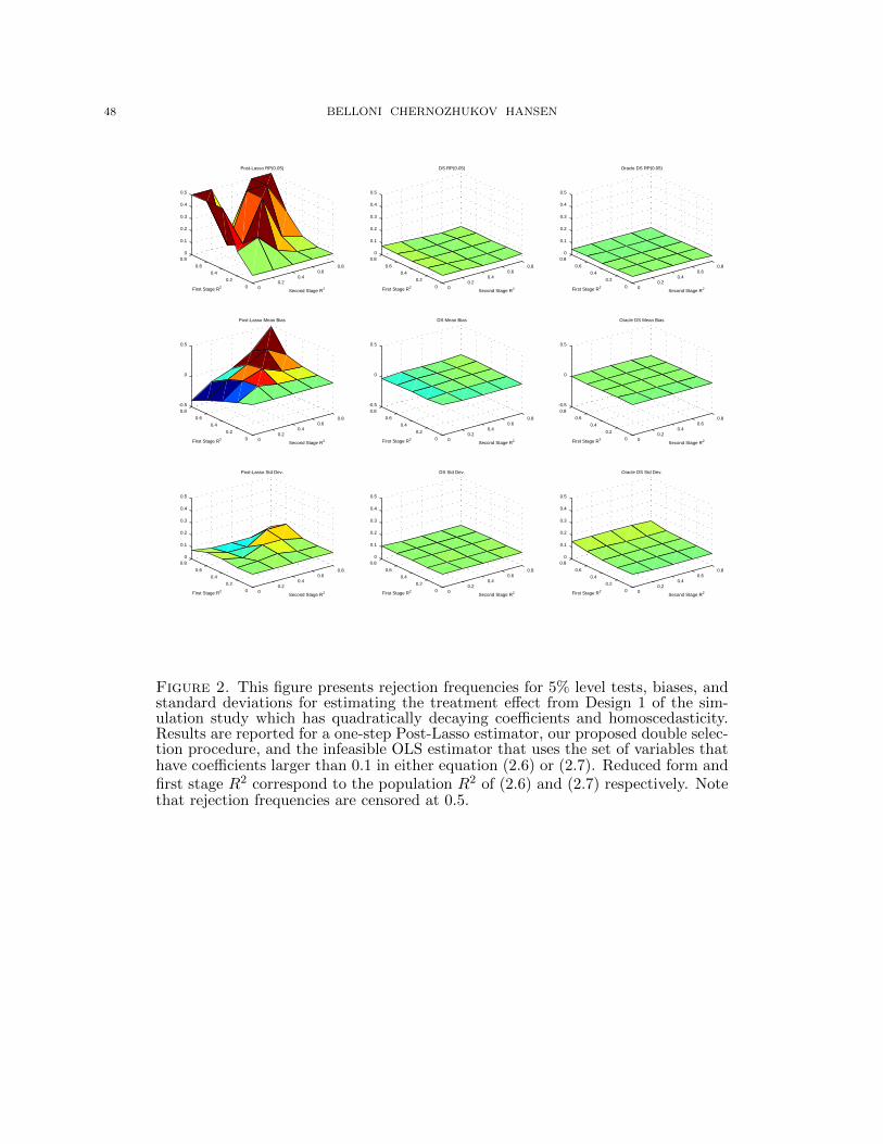
48 BELLONI CHERNOZHUKOV HANSEN
00.2
0.40.6
0.8
0
0.2
0.4
0.6
0.80
0.1
0.2
0.3
0.4
0.5
Second Stage R2
Post-Lasso RP(0.05)
First Stage R2
00.2
0.40.6
0.8
0
0.2
0.4
0.6
0.8-0.5
0
0.5
Second Stage R2
Post-Lasso Mean Bias
First Stage R2
00.2
0.40.6
0.8
0
0.2
0.4
0.6
0.80
0.1
0.2
0.3
0.4
0.5
Second Stage R2
Post-Lasso Std Dev.
First Stage R2
00.2
0.40.6
0.8
0
0.2
0.4
0.6
0.80
0.1
0.2
0.3
0.4
0.5
Second Stage R2
DS RP(0.05)
First Stage R2
00.2
0.40.6
0.8
0
0.2
0.4
0.6
0.8-0.5
0
0.5
Second Stage R2
DS Mean Bias
First Stage R2
00.2
0.40.6
0.8
0
0.2
0.4
0.6
0.80
0.1
0.2
0.3
0.4
0.5
Second Stage R2
DS Std Dev.
First Stage R2
00.2
0.40.6
0.8
0
0.2
0.4
0.6
0.80
0.1
0.2
0.3
0.4
0.5
Second Stage R2
Oracle DS RP(0.05)
First Stage R2
00.2
0.40.6
0.8
0
0.2
0.4
0.6
0.8-0.5
0
0.5
Second Stage R2
Oracle DS Mean Bias
First Stage R2
00.2
0.40.6
0.8
0
0.2
0.4
0.6
0.80
0.1
0.2
0.3
0.4
0.5
Second Stage R2
Oracle DS Std Dev.
First Stage R2
Figure 2. This figure presents rejection frequencies for 5% level tests, biases, andstandard deviations for estimating the treatment effect from Design 1 of the sim-ulation study which has quadratically decaying coefficients and homoscedasticity.Results are reported for a one-step Post-Lasso estimator, our proposed double selec-tion procedure, and the infeasible OLS estimator that uses the set of variables thathave coefficients larger than 0.1 in either equation (2.6) or (2.7). Reduced form andfirst stage R2 correspond to the population R2 of (2.6) and (2.7) respectively. Notethat rejection frequencies are censored at 0.5.

INFERENCE AFTER MODEL SELECTION 49
00.2
0.40.6
0
0.5
0
0.1
0.2
0.3
0.4
Second Stage R2
Post-Lasso RP(0.05)
First Stage R2
00.2
0.40.6
0
0.5
-0.5
0
0.5
Second Stage R2
Post-Lasso Mean Bias
First Stage R2
00.2
0.40.6
0
0.5
0
0.1
0.2
0.3
0.4
Second Stage R2
Post-Lasso Std Dev.
First Stage R2
00.2
0.40.6
0
0.5
0
0.1
0.2
0.3
0.4
Second Stage R2
DS RP(0.05)
First Stage R2
00.2
0.40.6
0
0.5
-0.5
0
0.5
Second Stage R2
DS Mean Bias
First Stage R2
00.2
0.40.6
0
0.5
0
0.1
0.2
0.3
0.4
Second Stage R2
DS Std Dev.
First Stage R2
00.2
0.40.6
0
0.5
0
0.1
0.2
0.3
0.4
Second Stage R2
Oracle DS RP(0.05)
First Stage R2
00.2
0.40.6
0
0.5
-0.5
0
0.5
Second Stage R2
Oracle DS Mean Bias
First Stage R2
00.2
0.40.6
0
0.5
0
0.1
0.2
0.3
0.4
Second Stage R2
Oracle DS Std Dev.
First Stage R2
Figure 3. This figure presents rejection frequencies for 5% level tests, biases, andstandard deviations for estimating the treatment effect from Design 2 of the sim-ulation study which has quadratically decaying coefficients and heteroscedasticity.Results are reported for a one-step Post-Lasso estimator, our proposed double selec-tion procedure, and the infeasible OLS estimator that uses the set of variables thathave coefficients larger than 0.1 in either equation (2.6) or (2.7). Reduced form andfirst stage R2 correspond to the population R2 of (2.6) and (2.7) respectively. Notethat rejection frequencies are censored at 0.5.
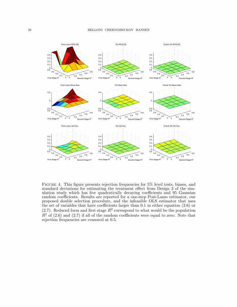
50 BELLONI CHERNOZHUKOV HANSEN
00.2
0.40.6
0.8
00.2
0.40.6
0.80
0.1
0.2
0.3
0.4
Second Stage R2
Post-Lasso RP(0.05)
First Stage R2
00.2
0.40.6
0.8
00.2
0.40.6
0.8-0.5
0
0.5
Second Stage R2
Post-Lasso Mean Bias
First Stage R2
00.2
0.40.6
0.8
00.2
0.40.6
0.80
0.1
0.2
0.3
0.4
Second Stage R2
Post-Lasso Std Dev.
First Stage R2
00.2
0.40.6
0.8
00.2
0.40.6
0.80
0.1
0.2
0.3
0.4
Second Stage R2
DS RP(0.05)
First Stage R2
00.2
0.40.6
0.8
00.2
0.40.6
0.8-0.5
0
0.5
Second Stage R2
DS Mean Bias
First Stage R2
00.2
0.40.6
0.8
00.2
0.40.6
0.80
0.1
0.2
0.3
0.4
Second Stage R2
DS Std Dev.
First Stage R2
00.2
0.40.6
0.8
00.2
0.40.6
0.80
0.1
0.2
0.3
0.4
Second Stage R2
Oracle DS RP(0.05)
First Stage R2
00.2
0.40.6
0.8
00.2
0.40.6
0.8-0.5
0
0.5
Second Stage R2
Oracle DS Mean Bias
First Stage R2
00.2
0.40.6
0.8
00.2
0.40.6
0.80
0.1
0.2
0.3
0.4
Second Stage R2
Oracle DS Std Dev.
First Stage R2
Figure 4. This figure presents rejection frequencies for 5% level tests, biases, andstandard deviations for estimating the treatment effect from Design 3 of the sim-ulation study which has five quadratically decaying coefficients and 95 Gaussianrandom coefficients. Results are reported for a one-step Post-Lasso estimator, ourproposed double selection procedure, and the infeasible OLS estimator that usesthe set of variables that have coefficients larger than 0.1 in either equation (2.6) or(2.7). Reduced form and first stage R2 correspond to what would be the populationR2 of (2.6) and (2.7) if all of the random coefficients were equal to zero. Note thatrejection frequencies are censored at 0.5.

INFERENCE AFTER MODEL SELECTION 51
00.2
0.40.6
0.8
00.2
0.40.6
0.80
0.05
0.1
Second Stage R2
DS RP(0.05)
First Stage R2
00.2
0.40.6
0.8
00.2
0.40.6
0.80
0.1
0.2
0.3
Second Stage R2
DS RMSE
First Stage R2
00.2
0.40.6
0.8
00.2
0.40.6
0.80
0.05
0.1
Second Stage R2
DS RP(0.05) (Ridge)
First Stage R2
00.2
0.40.6
0.8
00.2
0.40.6
0.80
0.1
0.2
0.3
Second Stage R2
DS RMSE (Ridge)
First Stage R2
Figure 5. This figure presents rejection frequencies for 5% level tests and RMSE’sfor estimating the treatment effect from Design 3 of the simulation study which hasfive quadratically decaying coefficients and 95 Gaussian random coefficients. Resultsin the first column are for the proposed double selection procedure, and the resultsin the second column are for the proposed double selection procedure when the ridgefit from (2.6) is added as an additional potential control. Reduced form and firststage R2 correspond to what would be the population R2 of (2.6) and (2.7) if allof the random coefficients were equal to zero. Note that the vertical axis on therejection frequency graph is from 0 to 0.1.

52 BELLONI CHERNOZHUKOV HANSEN
Effect Std. Err. Effect Std. Err. Effect Std. Err.
Donohue III and Levitt (2001) Table IV ‐0.129 0.024 ‐0.091 0.018 ‐0.121 0.047
First‐Difference ‐0.152 0.034 ‐0.108 0.022 ‐0.204 0.068
All Controls 0.014 0.719 ‐0.195 0.225 2.343 2.798
Post‐Double‐Selection ‐0.104 0.107 ‐0.030 0.055 ‐0.125 0.151
Post‐Double‐Selection+ ‐0.082 0.106 ‐0.031 0.057 ‐0.068 0.200
Note: The table displays the estimated coefficient on the abortion rate, "Effect," and its estimated standard error. Numbers in the
first row are taken from Donohue III and Levitt (2001) Table IV, columns (2), (4), and (6). The remaining rows are estimated by first
differences, include a full set of time dummies, and use standard errors clustered at the state‐level. Estimates in the row labeled
"First‐Difference" are obtained using the same controls as in the first row. Estimates in the row labeled "All Controls" use 284
control variables as discussed in the text. Estimates in the row "Post‐Double‐Selection" use the variable selection technique
developed in this paper to search among the set of 284 potential controls. Estimates in the row "Post‐Double‐Selection+" use the
variables selected by the procedure of this paper augmented with the set of variables from Donohue III and Levitt (2001).
Table 2. Estimated Effects of Abortion on Crime Rates
Violent Crime Property Crime Murder
A. Donohue III and Levitt (2001) Table IV