1

INFANT AND CHILD MORTALITY IN DEVELOPING COUNTRIES: ANALYSING

THE DATA FOR ROBUST DETERMINANTS

LUCIA HANMERDepartment for International Development, London (l-hanmer@dfid.gov.uk)

ROBERT LENSINK University of Groningen (b.w.lensink@eco.rug.nl)

AND

HOWARD WHITE* Institute of Development Studies, University of Sussex (h.white@ids.ac.uk)

Abstract

Is development best achieved by going for growth, or does specific attention needto be paid to directly improving human welfare? In contrast to the HumanDevelopment Reports of the UNDP, the World Bank has stressed the growthapproach. Recent work has reinforced this position by arguing that healthspending is extremely ineffective in reducing infant or child mortality, which ismainly explained by a country’s income per capita. This paper contests thisposition through testing the robustness of determinants of infant and childmortality. We have estimated over 420,000 equations which show that, whilstincome per capita is a robust determinant of infant and child mortality, so areindicators of health, education and gender inequality. Some health spending,such as immunisation, is thus shown to be a cost effective way of saving lives.Our results are consistent with the view that much health spending in developingcountries may be poorly targeted or otherwise ineffective, but do not support theposition that public health strategies should not be given too great a role inpursuing improvements in human welfare.

1. INTRODUCTION

There is widespread agreement that development should be measured by variables other than

GNP per capita. Health variables, such as infant or maternal mortality, and education

indicators, such as literacy, should be used to indicate a country’s developmental status. The

focus on non-income dimension of development was promoted through the Basic Needs

agenda in the 1970s, and the composite Physical Quality of Life Index. Since 1990, UNDP

has strongly advocated a similar position in its Human Development Reports (HDRs),

* Robert Lensink and Howard White are also Fellows of CREDIT, University of Nottingham. Thispaper is partly based on research carried out for Sida by Lucia Hanmer and Howard White. Thanks to

2

embodying the multi-dimensional view of development in the Human Development Index

(HDI). The International Development Targets, and the successor Millennium Development

Goals (MDGs), explicitly adopt a range of social goals, including reductions of two-thirds in

infant and under five mortality by 2015, as poverty reduction targets.1 But to agree that

measures of development should incorporate non-economic variables is not the same as

agreeing that achieving development requires looking beyond a growth-oriented development

strategy. Even if the objective is to maximise welfare as measured by social indicators, this

objective may arguably best be obtained by focussing on growth.

Two broad positions may be identified in this debate. In addition to directing

attention to non-economic welfare measures, the HDRs have typically pointed out that

countries at comparable levels of income per capita can have considerable variation in their

HDIs, suggesting that poor performers can raise welfare (i.e. improve social indicators)

without waiting for growth to do so. The 1996 HDR (and subsequent work in that vein by

Ramirez et al., 2000) went further to argue that, whilst investing in human capital can lay the

basis for subsequent growth, countries which have focused exclusively on economic growth

have, in the end, achieved neither sustained growth nor human development.

These views have been countered by Ravallion (1997) from the World Bank’s

research department. Ravallion admits that the relationship between social indicators and

income per capita is imperfect, but there is a relationship. Hence sustained improvements in

welfare are best brought about by increasing income - the main issue is, he suggests, not

whether growth is good or bad growth, but to get enough growth of any sort.2 A number of

Sida for funding are for useful comments at a seminar to present findings at a seminar in Stockholm.The usual disclaimer applies.1 Infant mortality is the probability of death in the first 12 months of life, and child mortality theprobability between first and five birthdays. Under five mortality is the probability of death betweenbirth and fifth birthday. Under five mortality thus conflates infant and child mortality. Since thedeterminants of these two are seen to be rather different demographers are not keen on under fivemortality as a measure. 2 For a longer discussion of these contrasting positions see White (1999).

3

other pieces of work emanating from the World Bank also emphasise a growth-led

development strategy. For example, Dollar and Kraay’s (2000) analysis of pro-poor argues

that spending on basic services is not pro-poor.3 Of direct relevance to our paper is analysis

by the World Bank’s research department (Filmer and Pritchett, 1997) on the determinants of

infant and child mortality. Specifically they argue that virtually all inter-country variation in

child mortality is explained by a set of development indicators including GNP per capita.

They seek to show that adding health expenditure to the model adds little explanatory power.

They therefore warn against supporting expanding public health services as a means to

improving welfare, thus implicitly supporting the view that growth is the answer. This paper

challenges these results.

We are well aware that this debate is not a new one. McKeown (1976) sought to

argue that medical advances had played little role in mortality reductions in England since the

eighteenth century. Whilst there is agreement that “specific therapeutic medical treatments

have played a minor role in mortality reductions in Western countries.. relatively little else of

the McKoewn thesis has survived” (Preston, 1996: 532). The weight of the evidence suggests

that public health measures, such as smallpox vaccination and the purification of milk, played

an important role (see Preston, 1996 for a review of the debate). Analysis of various

developing countries also showed “the pivotal role played by government programmes in

speeding mortality improvements” (Preston, 1996: 533). The only real debate concerned the

sources of low and declining mortality in Sri Lanka, with the “best estimate” suggesting that

close to half the reduction from 1930 to 1960 can be attributed to the anti-malaria programme

(Preston, 1996: 533). Our purpose here is to restate and strengthen the case for active social

policy by presentation of robust regression analysis applied to cross-country regressions in

Part 4.

3 This result is hardly surprising since they are seeking to explain income growth of the poor, which isunlikely to be affected by current government social spending.

4

We begin in Part 2 with some preliminary data analysis. This analysis confirms that

the link between income and infant mortality is an imperfect one – thus raising the question of

what may be done to strengthen it. It also shows that there has been a historical decline in

infant mortality over and above that which can be explained by income growth. To identify

other factors, in Part 3 we present a brief review of the literature on the determinants of infant

and child mortality. This review shows that these variables have been regressed on a wide

range of independent variables with differing results. Following the approach that has been

adopted in the growth literature (Sala-i-Martin, 1997) the appropriate response to such a

situation is to test the robustness of the coefficients of the variables of interest by estimating

all possible regression equations. This analysis, presented in Part 4, finds a robustly

significant impact on both infant and child mortality from some of the health variables in our

data set. Part 5 concludes.

2. SOME PRELIMINARY DATA ANALYSIS

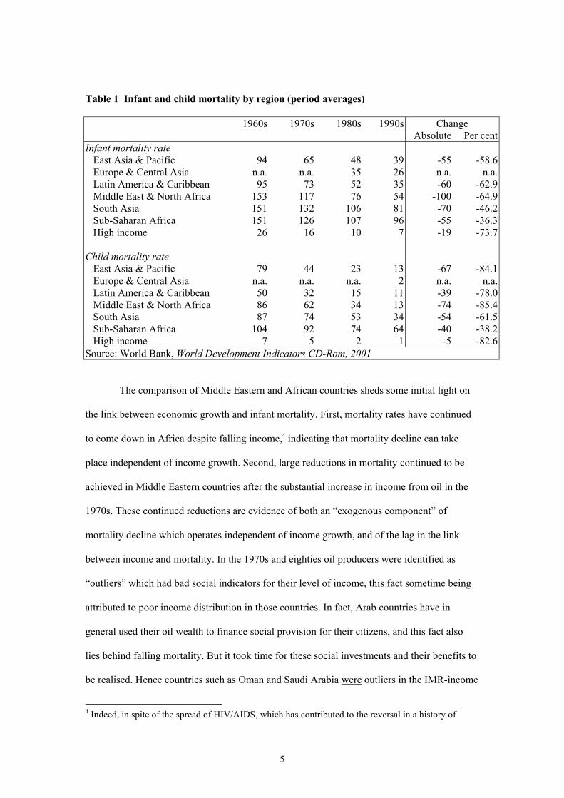
Table 1 shows infant and child mortality for developing countries classified by region. All

regions have recorded declines in both indicators. With respect to infant mortality, three

regions – the Middle East and North Africa, South Asia and sub-Saharan Africa – had similar

levels in the 1960s. But by the 1990s the rate for Africa was nearly double that in the Middle

East. These discrepancies in performance, also evident in the child mortality data, have

several explanations. Of course the Middle East benefited from oil wealth which, with some

lag (about which we will say more in a moment), has been transformed into improved social

indicators. But Africa has suffered serious economic decline, with falling income per capita

for the region as whole since the 1980s.

5

Table 1 Infant and child mortality by region (period averages)

1960s 1970s 1980s 1990s ChangeAbsolute Per cent

Infant mortality rate East Asia & Pacific 94 65 48 39 -55 -58.6 Europe & Central Asia n.a. n.a. 35 26 n.a. n.a. Latin America & Caribbean 95 73 52 35 -60 -62.9 Middle East & North Africa 153 117 76 54 -100 -64.9 South Asia 151 132 106 81 -70 -46.2 Sub-Saharan Africa 151 126 107 96 -55 -36.3 High income 26 16 10 7 -19 -73.7

Child mortality rate East Asia & Pacific 79 44 23 13 -67 -84.1 Europe & Central Asia n.a. n.a. n.a. 2 n.a. n.a. Latin America & Caribbean 50 32 15 11 -39 -78.0 Middle East & North Africa 86 62 34 13 -74 -85.4 South Asia 87 74 53 34 -54 -61.5 Sub-Saharan Africa 104 92 74 64 -40 -38.2 High income 7 5 2 1 -5 -82.6Source: World Bank, World Development Indicators CD-Rom, 2001

The comparison of Middle Eastern and African countries sheds some initial light on

the link between economic growth and infant mortality. First, mortality rates have continued

to come down in Africa despite falling income,4 indicating that mortality decline can take

place independent of income growth. Second, large reductions in mortality continued to be

achieved in Middle Eastern countries after the substantial increase in income from oil in the

1970s. These continued reductions are evidence of both an “exogenous component” of

mortality decline which operates independent of income growth, and of the lag in the link

between income and mortality. In the 1970s and eighties oil producers were identified as

“outliers” which had bad social indicators for their level of income, this fact sometime being

attributed to poor income distribution in those countries. In fact, Arab countries have in

general used their oil wealth to finance social provision for their citizens, and this fact also

lies behind falling mortality. But it took time for these social investments and their benefits to

be realised. Hence countries such as Oman and Saudi Arabia were outliers in the IMR-income

4 Indeed, in spite of the spread of HIV/AIDS, which has contributed to the reversal in a history of

6

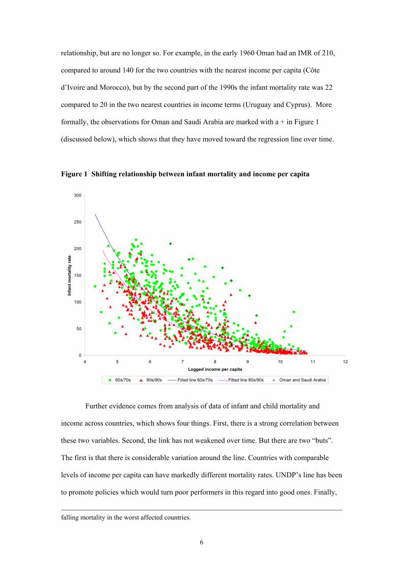
relationship, but are no longer so. For example, in the early 1960 Oman had an IMR of 210,

compared to around 140 for the two countries with the nearest income per capita (Côte

d’Ivoire and Morocco), but by the second part of the 1990s the infant mortality rate was 22

compared to 20 in the two nearest countries in income terms (Uruguay and Cyprus). More

formally, the observations for Oman and Saudi Arabia are marked with a + in Figure 1

(discussed below), which shows that they have moved toward the regression line over time.

Figure 1 Shifting relationship between infant mortality and income per capita

Further evidence comes from analysis of data of infant and child mortality and

income across countries, which shows four things. First, there is a strong correlation between

these two variables. Second, the link has not weakened over time. But there are two “buts”.

The first is that there is considerable variation around the line. Countries with comparable

levels of income per capita can have markedly different mortality rates. UNDP’s line has been

to promote policies which would turn poor performers in this regard into good ones. Finally,

falling mortality in the worst affected countries.

0

50

100

150

200

250

300

4 5 6 7 8 9 10 11 12

Logged income per capita

Infa

nt m

orta

lity

rate

60s/70s 80s/90s Fiited line 60s/70s Fitted line 80s/90s Oman and Saudi Arabia

7

the regression relationship has shifted over time, giving exogenous changes in mortality not

explained by income growth. These points can be seen from Figure 1, which is based on data

for 115 countries each with eight observations, using seven five year periods from 1960-64 to

1990-94 and the last being 1995-97. Only countries with data on infant mortality and income

for all periods are included, so that shifts in the regression relationship cannot be accounted

for by countries being added to, or dropped from, the sample.5

The estimated coefficient from the simple double-log regression of IMR on income

per capita is –0.52.6 The data clearly show that there has been a “downward drift” in the

observations over time, which applied to all income groups. That is, for an given income per

capita, a country will have a lower infant mortality rate at that income than it would have

twenty years ago. This fact is captured by estimating separate regression lines for the two

periods, the first sub-sample comprising the observations from the sixties and seventies and

the second sub-sample those from the eighties and nineties.7

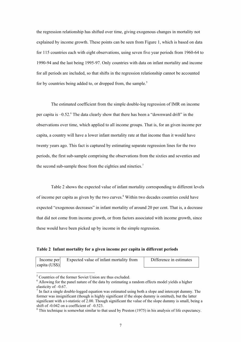
Table 2 shows the expected value of infant mortality corresponding to different levels

of income per capita as given by the two curves.8 Within two decades countries could have

expected “exogenous decreases” in infant mortality of around 20 per cent. That is, a decrease

that did not come from income growth, or from factors associated with income growth, since

these would have been picked up by income in the simple regression.

Table 2 Infant mortality for a given income per capita in different periods

Income percapita (US$)

Expected value of infant mortality from Difference in estimates

5 Countries of the former Soviet Union are thus excluded.6 Allowing for the panel nature of the data by estimating a random effects model yields a higherelasticity of –0.67.7 In fact a single double-logged equation was estimated using both a slope and intercept dummy. Theformer was insignificant (though is highly significant if the slope dummy is omitted), but the lattersignificant with a t-statistic of 2.00. Though significant the value of the slope dummy is small, being ashift of -0.042 on a coefficient of –0.523. 8 This technique is somewhat similar to that used by Preston (1975) in his analysis of life expectancy.

8

fitted line for sixtiesand seventies

fitted line for eightiesand nineties

Absolute Percentage

150 185 151 -34 -18.2 500 98 76 -22 -22.31,000 68 52 -17 -24.52,000 48 35 -13 -26.75,000 30 21 -9 -29.4

Our preliminary data analysis thus suggests two things. First, that at least some

reduction in infant mortality comes from factors other than income growth. Second, that the

strength and timing of the link between income and reduced mortality varies across time and

space. We turn now to analyse these points in more detail.

3. EXISTING LITERATURE AND THEORETICAL FRAMEWORK

Theoretical framework

There is a substantial literature in child health outcomes, as measured by both mortality and

morbidity, which mostly adopts something like the Mosley-Chen (1984) framework, depicted

in Figure 2. Myers (1994) comments that this framework “combines social science and

medical perspectives in a parsimonious way” (1994: 52-53). The insight of this approach is

that underlying socio-economic status (SES) manifests itself in (measurable) proximate

determinants. The values of these variables influence the risk of disease, which link to the

probability of death.

The Mosley-Chen model motivates the idea that countries with the same income per

capita will have differing mortality rates since the relationship is mediated in several ways.

For example, analysis of household data show a very strong relationship between mortality

and both preceding and succeeding birth interval. Hence higher fertility, which implies a

shorter birth interval, is associated with higher mortality. Fertility, in turn, is associated with

income, but imperfectly so as both cultural factors and livelihood strategies (crucially the

availability of alternative safety nets) play a role. So public policy to reduce fertility, either

9

through promotion of reproductive health or through the provision of reliable safety nets, will

bring down mortality.

Figure 2 The Mosley-Chen framework for analysing mortality

Risk ofdisease

Mortalityoutcomes

Socio-economicstatus (SES)

Social

Economic

Biological

Environmental

Proximate determinants

Maternal fertility

Environmentalcontamination

Nutrient availability

Injuries

Disease control

In practice, some aspects of socio-economic status variables may be used in empirical

estimation, either because they are seen to have direct impacts, or because data on these are

more readily available than the corresponding proximate variables. We identify the actual

variables to be used with reference to existing empirical work.

Empirical findings

The literature on infant and child mortality spans medical studies of different interventions,

anthropological studies of child rearing practices and regression analysis.9 Our attention here

is restricted to the latter (see Hanmer and White, 1998 for discussion of the other areas).

Regression analysis of the determinants of under five mortality may take one of four

approaches: (1) cross-country regressions, in which mortality is defined at the level of the

country as a whole; (2) cross country regressions for a single country with data for different

administrative units (e.g. districts); (3) analysis of survey data, mortality being defined with

reference to either a mother or individual child; and (4) time-series analysis for a single

country, using the national mortality rate as the dependent variable. The second area of

9 Infant mortality is the probability of death in the first 12 months, child mortality that between the firstand fifth birthdays, and that before the fifth birthday is under five mortality. These probabilities are

10

analysis became dominant with the availability of data first from the World Fertility Survey

(WFS) and later the demographic health survey (DHS), both of which have taken place in

many countries. These studies show fairly consistent patterns between demographic

determinants and mortality (e.g. a child’s sex and birth spacing) and rather less consistency in

socio-economic determinants. Early papers illustrating both these points using WFS data are

by Hobcraft et al. (1984 and 1985 respectively); see also , for example, Desai and Alva

(1998) for a recent analysis arguing that mother’s education is a significant determinant of

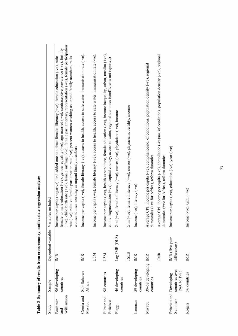
mortality only in some countries. However, our concern here is with cross-country

regressions, with the results of a selection of studies being summarised in Table 3.

Cross-country regressions typically combine income per capita with a range of other

variables for both SES and proximate determinants. One of the earliest and most common of

additional variables has been a measure of female education, typically female literacy, which

is often found to have a significant negative effect. This is consistent with the view strongly

advanced by Caldwell (e.g. 1986) that female education is an important mediating variable.

Since there is a high correlation between the female literacy and total literacy then total

literacy may work just as well. Many studies distinguish both male and female education,

sometimes finding both to be significant. Alternatively other measures of women’s status may

be used, which may indicate how much say mothers have over the allocation of resources.

Boehmer and Williamson (1996) find that several measures of women’s status to have a

significant impact.

The distribution of income, as well as its level, may be expected to matter.

Accordingly, several studies have found a significant impact from inequality. Interestingly

Waldmann (1992), finds that inequality still exerts an adverse impact on mortality even once

the real income of the poor is also included in the regression - though none of the hypothesis

as to why this may be so are supported by the data.

usually expressed per thousand live births.

11

An important channel through which improving socio-economic status can operate on

reducing mortality is through health and education. We have already mentioned that both

female and male education are often included. In addition a variety of health indicators have

been used, such as contraceptive prevalence and the number of persons per physician, finding

a significant impact from health provision on under five mortality. The exception is the study

by Filmer and Pritchett (1997), in which health expenditure is significant only at the 10 per

cent level. As mentioned in the introduction, strong policy conclusions are drawn by Filmer

and Pritchett from their analysis. Given these contrasting results, what conclusions should in

fact be drawn?

Table 3 reports more than twenty variables which have been used as determinants of

infant and child mortality. Other studies not shown here have used yet more variables. The

significance of most of these variables, including income per capita, varies between studies.

That is, the results are not robust. Findings vary according to both model specification and the

sample used. Lack of robustness with respect to model specification means that a variable

appears to be significant when included with some sets of regressors, but not with others. This

problem has been apparent in regression analysis of the determinants of growth for some

time, and the technique used has been to examine robustness by examining all possible sets of

regressors (also called fragility analysis). This brief review suggests that the literature on the

determinants of infant and child mortality would benefit from such an approach, and it is to

this we now turn.

12

4. SOME REGRESSION RESULTS

Methodology

In this section we test which variables have a robust effect on child and infant mortality using

the method introduced by Sala-i-Martin (1997).10 He specifies a regression equation of the

following form:

Y I M ZI j M j Z j= + + + +α β β β ε, , , (1)

where Y is a vector of dependent variables (in our case child and infant mortality, CMR and

IMR respectively, both of which are for 1995); I is a set of variables always included in the

regressions, M are other variables of interest and Z a vector of additional variables which may

potentially be important explanatory variables of infant or child mortality. Defining I

variables reduces the number of regressions which have to be performed, which is equal to

Number of equationsM Z

M Z k kM=

++ −

( )!( )! !

(2)

where k is the number of regressors included in each equation.11

We estimated equation (1) using three data sets. A number of variables are excluded

from the first data set on account of missing observations, thus allowing a larger sample size.

For reasons of comparability across estimated equations, we only include observations for

which all variables in that data set are available. In this data set the intercept and the log of

GNP per capita were taken as I variables (i.e. included in all regressions). The M variables

(those we are particularly interested in, which in our case are all indicators of social policy) in

the three data sets are12:

10 There are a number of tests for robustness which may be used. The first, as used by Levine, is to saya variable is fragile if it is insignificant in just one of the estimated regressions. This test is clearly avery tough one (which would be passed by none of the variables in our analysis). A second alternative,also used by Sala-i-Matin is to examine what proportion of times a variable is significant, taking it tobe robust if it is so in 90 or 95 per cent of cases.11 In order to have a manageable number of regressions we have restricted each equation to fourregressors (plus the I variables), which accounts for the formula given here.12 We would like to have also included a measure of income inequality. Although such data areavailable for an increasing number of countries these turn out not to be the same countries for whichour other data were available, so the income inequality measure was excluded.

13

• education variables: literacy in 1995 (LIT95), female literacy in 1995 (FLIT95), male

primary school enrolment in 1960 (PSERM60), female primary school enrolment in 1960

(PSERF60), male primary school enrolment in 1990 (PSERM90), female primary school

enrolment in 1990 (PSERF90), male and female secondary school enrolments in 1960

(SSERM60 and SSERF60), and male and female secondary school enrolments in 1990

(SSERM90 and SSERF90)

• health variables: DPT immunisation rate in 1995 (DPT95), polio immunisation in 1995

(P95), measles immunisation (M95), TB immunisation in 1995 (TB95), percentage of

births attended by trained health staff (BIRTHADD), proportion low birth weight children

(LBW, 2nd data set only), HIV/AIDS prevalence rates (AIDS, 2nd data set only), access to

safe water (WACC, 2nd data set only), access to sanitation (SACC, 2nd data set only),

population per physician (3rd data set only), population per nurse (3rd data set only) and the

ratio of physicians to nurses (DNRATIO, 3rd data set only).

• gender equality variables:13 the ratio of female to male primary school enrolment in 1990

(PSERFM), the ratio of female to male secondary school enrolment in 1990 (SSERFM),

the ratio of female to male life expectancy (LEFM) and the same ratio for literacy

(LITFM).

The other variables included in the data set (the Z variables) are population, an African

dummy, contraceptive prevalence, the crude birth rate (lagged by five years), total fertility

rate, the ratio of child to infant morality and the degree of urbanisation.

13 An earlier version of this paper found that gender inequality, expressed as the ratio of the gender andhuman development indices (GDI/HDI) to be a robust determinant for infant and child mortality.However, it appeared preferable to break the index down to its component parts.

14

The estimation procedure is as follows. For each M variable, we estimated all

possible combinations of four of the remaining group of 24 independent variables (i.e. all 17

M and all 7 Z variables). This means that for each M variable 10,626 (=24!/(20! 4!))

equations are estimated. The I variables (LGNP and a constant) are included in all equations.

From these estimates, the mean estimate of β(M) and the average variance of these estimates

are calculated as:

nianceiance

nM

/varvar

/)(

Σ=

Σ= ββ(3)

where n is the number of estimates of estimated coefficients (10,626 in this case). A variable

is said to be robust if 95 per cent of the estimated coefficients have the same sign.

Equivalently, the statistics from equation (3) are used to test whether the β(M) is significantly

different from 0 using the standard z tests (which therefore assumes that the estimated βs are

normally distributed). A one-tail test (thus giving an absolute critical value of 1.64) of the null

hypothesis (that β=0) is carried out. If the null is rejected (i.e. | z | >1.64) then the coefficient

in question is said to be robust.

However, before applying the above procedure to the M variables, we tested whether

LGNP has a robust effect, as only under such circumstances is it justified to include LGNP as

a fixed variable (i.e. an I variable). This test was carried out using the approach outlined

above, but with the difference is that only the constant is an I variable. Hence, for LGNP

12,650 = (25!/(21! 4!)) equations have been estimated. The results shown in Table 4 show

that LGNP has a robust effect on both CMR and IMR, hence it is valid to use it as an I

variable. The table also shows the cumulative distribution (CDF) which is the per cent of

estimates laying to one side of the zero. In the case of GNP this figure is 99 per cent for CMR

and 100 per cent for IMR.

Results

15

Table 4 also reports the results for the other M variables in the first data set. The

variables are listed in order of their significance in each case. In addition to income per capita,

variables from each of three areas - health, education and gender inequality - are found to be

robust. For health, TB immunisation significantly reduces both infant and child mortality, and

immunisation against measles reduces child mortality. Let us be clear what these results

mean. Whilst it is possible to find a regression in which, say TB immunisation, has an

insignificant impact on child mortality, such regressions are only 3 per cent of the over

10,000 regressions we estimated which include that variable. It is important to bear in mind

the distinction between data analysis and data mining. The data miner knows the result they

are looking for and stops when they find it (and reports that result), whereas the data analyst

is looking for the story which is most consistent with the data.14 Robust regression is a tool of

a data analyst, which in this case clearly shows that the view that health interventions matter

for child survival is the story most consistent with the data.

None of the 1960 education variables are robustly significant, but both male and

female primary enrolments in 1990 are robust determinants of child mortality and, rather

surprisingly, male secondary enrolments are robust determinants of infant mortality. Gender

disparity in literacy has robust effect on both infant and child mortality and gender disparity

in life expectancy an adverse impact on child mortality. The sign in the former case is

negative as expected ( the higher the ratio of female to male literacy the lower the child

mortality), but the sign in the latter case is “wrong”.

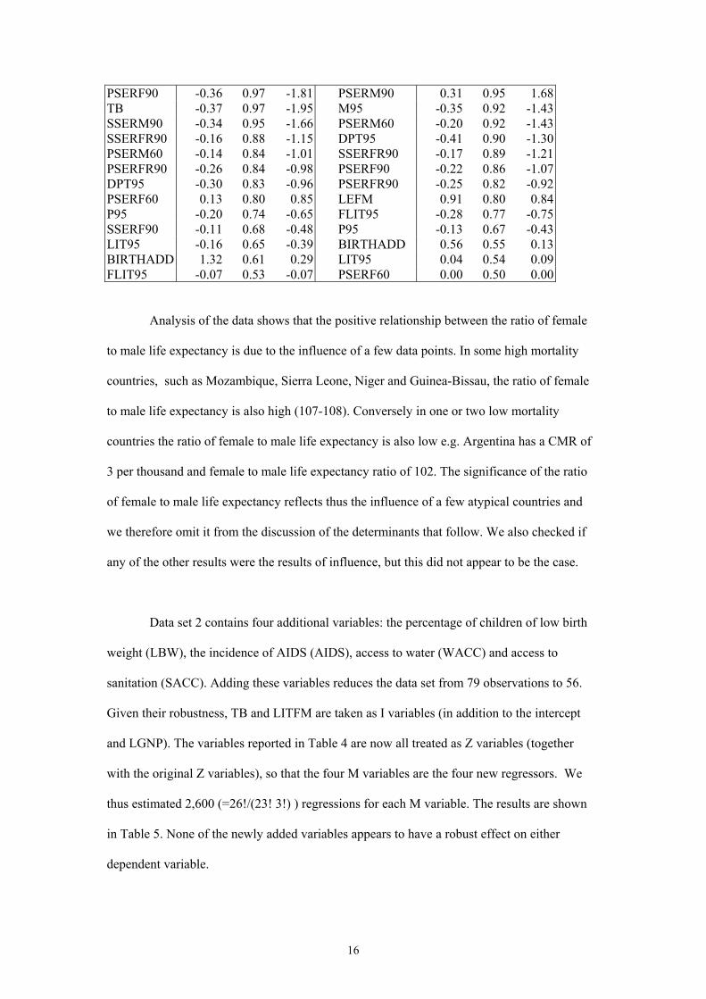
Table 4 Robustness tests for data set 1Variable Child Mortality Rate Variable Infant mortality rate

β CDF z-stat. β CDF z-stat.PSERM90 -0.46 1.00 -2.65 LGNP -11.54 1.00 <-3.99LGNP -8.58 0.99 -2.41 LITFM -0.68 1.00 -2.65LEFM 2.27 0.99 2.20 TB -0.49 1.00 -2.58LITFM -0.57 0.99 -2.26 SSERF90 -0.43 0.97 -1.81M95 -0.51 0.98 -2.15 SSERM90 -0.37 0.96 -1.76

14 Since Mukherjee et al. (1998) and White (2002) for further discussion of these ideas.

16

PSERF90 -0.36 0.97 -1.81 PSERM90 0.31 0.95 1.68TB -0.37 0.97 -1.95 M95 -0.35 0.92 -1.43SSERM90 -0.34 0.95 -1.66 PSERM60 -0.20 0.92 -1.43SSERFR90 -0.16 0.88 -1.15 DPT95 -0.41 0.90 -1.30PSERM60 -0.14 0.84 -1.01 SSERFR90 -0.17 0.89 -1.21PSERFR90 -0.26 0.84 -0.98 PSERF90 -0.22 0.86 -1.07DPT95 -0.30 0.83 -0.96 PSERFR90 -0.25 0.82 -0.92PSERF60 0.13 0.80 0.85 LEFM 0.91 0.80 0.84P95 -0.20 0.74 -0.65 FLIT95 -0.28 0.77 -0.75SSERF90 -0.11 0.68 -0.48 P95 -0.13 0.67 -0.43LIT95 -0.16 0.65 -0.39 BIRTHADD 0.56 0.55 0.13BIRTHADD 1.32 0.61 0.29 LIT95 0.04 0.54 0.09FLIT95 -0.07 0.53 -0.07 PSERF60 0.00 0.50 0.00

Analysis of the data shows that the positive relationship between the ratio of female

to male life expectancy is due to the influence of a few data points. In some high mortality

countries, such as Mozambique, Sierra Leone, Niger and Guinea-Bissau, the ratio of female

to male life expectancy is also high (107-108). Conversely in one or two low mortality

countries the ratio of female to male life expectancy is also low e.g. Argentina has a CMR of

3 per thousand and female to male life expectancy ratio of 102. The significance of the ratio

of female to male life expectancy reflects thus the influence of a few atypical countries and

we therefore omit it from the discussion of the determinants that follow. We also checked if

any of the other results were the results of influence, but this did not appear to be the case.

Data set 2 contains four additional variables: the percentage of children of low birth

weight (LBW), the incidence of AIDS (AIDS), access to water (WACC) and access to

sanitation (SACC). Adding these variables reduces the data set from 79 observations to 56.

Given their robustness, TB and LITFM are taken as I variables (in addition to the intercept

and LGNP). The variables reported in Table 4 are now all treated as Z variables (together

with the original Z variables), so that the four M variables are the four new regressors. We

thus estimated 2,600 (=26!/(23! 3!) ) regressions for each M variable. The results are shown

in Table 5. None of the newly added variables appears to have a robust effect on either

dependent variable.

17

Table 5 Robustness tests for data set 2Child Mortality Rate Infant mortality Rate

β CDF z-statistic β CDF z-statisticLBW -0.46 0.85 -1.02 -0.09 0.58 -0.19AIDS 0.51 0.85 1.04 0.51 0.84 0.98WACC 0.001 0.50 0.00 -0.03 0.57 -0.16SACC -0.03 0.58 -0.21 -0.13 0.81 -0.93

The third data set adds a further three variables: population per physician

(DOCTOR), population per nurse (NURSE) and the ratio of doctors to nurses (DNRATIO).

The last of these is intended to give proxy for the relative importance of primary health

services. The data set is reduced to 38 observations. The I variables are as for data set 2, the

new variables are M variables, and the remaining regressors Z variables. There are 3,654 ( =

29! / (25! 3!) ) equations to be estimated for each M variable. The results, shown in Table 6,

indicate that DOCTOR does have a robust impact on both infant and child mortality (fewer

people per doctor reduces mortality), thus further bearing out the argument that health

services can make a difference.

Table 6 Robustness tests for data set 3Child Mortality Rate Infant Mortality Rate

β CDF z-statistic β CDF z-statisticDOCTOR 0.001 1.00 3.33 0.001 1.00 2.50NURSE 0.001 0.83 1.00 0.001 0.90 1.14DNRATIO -0.960 0.70 -0.52 0.470 0.59 0.23

Summary and interpretation

The robust regression approach involves estimating all possible sets of regressors.

Although we imposed some limit on the range of specifications , we have estimated over

200,000 regressions for each of child and infant mortality. Our results bear out that income

per capita is a robust determinant of both of these two variables, but so are indicators of each

of health, education and gender inequality. Our results thus support the majority of empirical

work which finds that health interventions can significantly affect infant and child health.

18

These findings are in contrast to those of Filmer and Pritchett (1997) who argue that

health spending has only a weak effect. Indeed they use their results to show that health

spending of between $50,000 and $100,000 is required to save a life, which compares with

typical estimates of the cost effectiveness of medical interventions of between $10 and

$4,000.15 Our results may be used for a similar cost effectiveness calculation. Using mean

values of the variables, our results suggest that just under one life is saved by the reduction in

child mortality brought about by the immunisation of three children. Supposing that

immunising one child (with all support costs) costs $10, then the cost per life saved is only

$30.16

How can this difference in results be explained? Filmer and Pritchett use total health

expenditure. As they themselves recognise, their results may thus pick up the ineffectiveness

of much health spending, which may be poorly targeted and spent on the wrong things, rather

than the ineffectiveness of medical interventions per se. This fact which makes their cost

effectiveness calculation somewhat misleading. For example, spending may go largely toward

tertiary institutions, which do little to bring down infant and child mortality. Also the cost of

delivering health services differs widely between countries, and these differences may drown

out the impact of health services, so that physical input and process measures, such as the

number of doctors and immunisation rates respectively, are more likely to show some

significant effect. Our results support these arguments since they show that some

interventions, such as immunisation, can indeed make a difference. However, our proxy for

the relative importance if primary health (DNRATIO) was not robust, suggesting that

refocusing on primary level services is not in itself sufficient.

15 Cornia and Mwabu (1997) also present the relative impact of different variables on mortality, buttheir calculations take no account of cost differences.16 It is difficult to get a meaningful figure for the “cost of immunisation” which depends on inter aliathe availability of health infrastructure and population density.

19

We should be clear that our results do not suggest that “money does not matter”.

Growth is clearly important. GNP per capita proved robust, although many of the other

variables we included pick up the channels through which higher income operates to reduce

mortality. Indeed, we fully recognise that growth is necessary to sustain expenditure on health

services. The main missing channel from our model specifications was the effect of income

on private consumption, which makes possible better nutrition and greater access to services.

This thus explains why income has a direct effect even though the other channels through

which it operates (e.g. lower fertility and more health and education) are included in the

model.

But we also find that education has an affect independent of income, supporting the

idea that it is an important mediating variable between income and mortality. Whilst higher

income is needed to sustain the expansion of quality education, attention has to be paid to

providing that education so that economic progress is translated into broader social

development. In this context it is worth noting that inequalities in female and male literacy are

bad for child survival prospects. Our results thus also support the well-established view that

female education matters for child health. There is thus a clear role for social policy in

education, as well as health provision, if development targets to reduce infant and child

mortality are to be realised.

20

5. CONCLUSION

Should countries wanting to promote human welfare focus on growth, or are specific social

interventions advisable? It might be thought obvious that whilst growth is necessary to

sustain welfare improvements, it alone is not necessary. An active social policy to address

basic needs will bring about a more rapid improvement in social indicators. However, recent

work by the World Bank has argued that health spending is a poor means of improving infant

and child morality. Our paper refutes that position. We show that not only is there

considerable variation in country mortality rates not explained by differences in income per

capita, but also that mortality reductions have been achieved independent of income growth.

In explaining why this is so, we show specific health interventions to be robust determinants

of these variables. Moreover, the results suggests that interventions such as immunisation are

a cost effective way of saving lives. These results are not inconsistent with the view that

health spending is poorly targeted, which would explain why health spending is insignificant

in other studies, whereas our measure of health services delivery are significant. Other factors,

such as cost differences may play a role in explaining the insignificance of health expenditure

in mortality regressions. We believe that the contention that health expenditure is an

inefficient means of improving child health is unproven. To the contrary, our results support

the importance of social policy if poverty reduction goals are to be achieved. However,

further work is required to identify the most effective interventions.

REFERENCES

Boehmer, Ulrike and John Williamson (1996) “The Impact of Women’s Status on InfantMortality Rate: a cross-national analysis” Social Indicators Research 37(2) 333-360.

Caldwell, J.C. (1986) “Routes to Low Mortality in Developing Countries” Population andDevelopment Review 12(2) 171-220.

Cornia, Giovanni Andrea and Germano Mwabu (1997) “Health Status and Health Policy insub-Saharan Africa: a long-term perspective” WIDER Working Paper 141 [Helsinki:WIDER].

Desai, Sonalde and Soumya Alva “Maternal Education and Child Health: is there a strongcausal relationship?” Demography 35(1) 71-81.

21

Filmer, Deon and Lant Pritchett (1997) “Child Mortality and Public Spending on Health: howmuch does money matter?” Policy Research Working Paper 1864 [Washington D.C.: WorldBank].

Flegg, A.T. (1982) “Inequality of income, illiteracy and medical care as determinants ofinfant mortality in underdeveloped countries” Population Studies 36 441-58.

Hanmer, Lucia and Howard White (1999) Human Development in Sub Saharan Africa [TheHague: Institute of Social Studies Advisory Service].

Hobcraft, J.N., J.W. McDonald and S.O. Rutstein (1984) “Socio-economic factors in infantand child mortality. A cross-country comparison” Population Studies 38 193-223.

Hobcraft, J.N., J.W. McDonald and S.O. Rutstein (1985) “Demographic determinants ofinfant and child mortality. A comparative analysis” Population Studies 39 363-385.

Isenman, P. (1980) “Basic Needs: the case of Sri Lanka” World Development 8 237-58.

McKeown, Thomas (1976) The Modern Rise of Population

Mukherjee, Chandan, Howard White and Marc Wuyts (1998) Econometrics and DataAnalysis for Developing Countries (with), 1998 [London: Routledge].

Mwabu, G. (1996) “Health effects of market-based reforms in developing countries” WIDERWorking Paper 120 [Helsinki: WIDER].

Myers

Preston, Samuel (1975) “The changing relation between mortality and level of economicdevelopment” Population Studies 29 231-248.

Preston, Samuel (1996) “Population Studies in Mortality” Population Studies 50 525-536.

Pritchett, Lant and Lawrence Summers (1996) “Wealthier is Happier” Journal of HumanResources 31(4) 841-868.

Ramirez, Alejandro, Gustav Ranis and Frances Stewart (2000) “Economic Growth andHuman Development”, World Development

Ravallion, Martin (1997) “Good and Bad Growth: the Human Development Reports” WorldDevelopment 25(5) 631-638.

Rodgers, G.B. (1979) “Income and Inequality as Determinants of Mortality: an internationalcross-section analysis” Population Studies 33(2) 343-51.

Sala-i-Martin, XX (1997) “I Just Ran Two Million Regressions”, American Economic Review87(2) 178-183.

Singh, R.D. (1984) “Fertility-mortality variations across LDCs: women’s education, labourforce participation and contraceptive use” Kyklos 47(2) 209-229.

Subbarao, K. and Kaura Raney (1995) “Social Gains from Female Education: a cross-nationalstudy” Economic Development and Social Change 44(1) 105-127.

22

Waldmann, R.J. (1992) “Income Distribution and Infant Mortality” Quarterly Journal ofEconomics 1283-1302.

White, Howard (1999) “Global poverty reduction: are we heading in the right direction?”,Journal of International Development 11.

White, Howard (2002) “Combining quantitative and qualitative approaches in povertyanalysis”, World Development

23

Tab

le 3

Sum

mar

y of

res

ults

from

cro

ss-c

ount

ry m

utliv

aria

te r

egre

ssio

n an

alys

es

Stud

ySa

mpl

eD

epen

dent

var

iabl

eV

aria

bles

incl

uded

Boe

hmer

and

Will

iam

son

96 d

evel

opin

gco

untri

esIM

RIn

com

e pe

r cap

ita (n

egat

ive)

; and

add

ed o

ne a

t a ti

me:

fem

ale

illite

racy

(+ve

), fe

mal

e ed

ucat

ion

(-ve

), ra

tiofe

mal

e to

mal

e ed

ucat

ion

(-ve

), ge

nder

equ

ality

(-ve

), ag

e m

arrie

d (-

ve),

cont

race

ptiv

e pr

eval

ence

(-ve

), fe

rtilit

y(+

ve),

child

birt

h ra

te (+

ve),

fem

ale

suff

rage

(-ve

), fe

mal

e pa

rliam

enta

ry re

pres

enta

tion

(-ve

), fe

mal

e pa

rtici

patio

nra

te (-

ve),

rela

tive

fem

ale

parti

cipa

tion

rate

(-ve

), pe

rcen

t wom

en w

orki

ng a

s unp

aid

fam

ily m

embe

rs, r

atio

wom

en to

men

wor

king

as u

npai

d fa

mily

mem

bers

Cor

nia

and

Mw

abu

Sub-

Saha

ran

Afr

ica

IMR

Inco

me

per c

apita

(-ve

), fe

mal

e lit

erac

y (-

ve),

acce

ss to

hea

lth, a

cces

s to

safe

wat

er, i

mm

unis

atio

n ra

te (-

ve).

U5M

Inco

me

per c

apita

(-ve

), fe

mal

e lit

erac

y (-

ve),

acce

ss to

hea

lth, a

cces

s to

safe

wat

er, i

mm

unis

atio

n ra

te (-

ve).

Film

er a

ndPr

itche

et98

cou

ntrie

sU

5MIn

com

e pe

r cap

ita (-

ve),

heal

th e

xpen

ditu

re, f

emal

e ed

ucat

ion

(-ve

), in

com

e in

equa

lity,

urb

an, m

uslim

(+ve

),et

hnic

frag

men

tatio

n (+

ve),

tropi

cal c

ount

ry, a

cces

s to

wat

er, r

egio

nal d

umm

ies (

coef

ficie

nts n

ot re

porte

d)

Fleg

g46

dev

elop

ing

coun

tries

Log

IMR

(OLS

)G

ini (

+ve)

, fem

ale

illite

racy

(+ve

), nu

rses

(-ve

), ph

ysic

ians

(-ve

), in

com

e

TSLS

Gin

i (+v

e), f

emal

e ill

itera

cy (+

ve),

nurs

es (-

ve),

phys

icia

ns, f

ertil

ity, i

ncom

e

Isen

man

59 d

evel

opin

gco

untri

esIM

R

Inco

me

(-ve

), lit

erac

y (-

ve)

Mw

abu

39-6

8 de

velo

ping

coun

tries

IMR

Ave

rage

CPI

, inc

ome

per c

apita

(-ve

), co

mpl

ianc

e/no

. of c

ondi

tions

, pop

ulat

ion

dens

ity (-

ve),

regi

onal

dum

mm

ies (

+ve

for A

fric

a), r

efor

m d

umm

ies

CM

RA

vera

ge C

PI, i

ncom

e pe

r cap

ita (-

ve),

com

plia

nce

(-ve

)/no.

of c

ondi

tions

, pop

ulat

ion

dens

ity (-

ve),

regi

onal

dum

mm

ies (

+ve

for A

fric

a), r

efor

m d

umm

ies

Pritc

hett

and

Sum

mer

sD

evel

opin

gco

untri

es o

ver

1960

to 1

985

IMR

(fiv

e ye

ardi

ffer

ence

s)In

com

e pe

r cap

ita (-

ve),

educ

atio

n (-

ve),

year

(-ve

)

Rog

ers

56 c

ount

ries

IMR

Inco

me

(-ve

), G

ini (

+ve)

24

Dev

elop

ing

coun

try su

b-sa

mpl

eIn

com

e (-

ve),

Gin

i

Sing

h25

-32

deve

lopi

ngco

untri

esIM

RFe

mal

e ed

ucat

ion/

liter

acy

(-ve

), fe

mal

e la

bour

par

ticip

atio

n (-

ve),

GN

P pe

r cap

ita, %

wom

en h

eade

d ho

useh

olds

(+ve

), %

atte

nded

birt

hs (-

ve),

relig

ious

dum

my.

Subb

arao

and

Ran

ey72

dev

elop

ing

coun

tries

IMR

Fem

ale

enro

lmen

t (-v

e), m

ale

enro

lmen

t, fa

mily

pla

nnin

g se

rvic

es (-

ve),

inco

me

per c

apita

(-ve

), po

pula

tion

per

phys

icia

n (+

ve),

rate

of u

rban

isat

ion

(+ve

), re

gion

al d

umm

ies

Not

es: (

+ve)

and

(-ve

) ind

icat

e si

gnifi

cant

pos

itive

and

neg

ativ

e re

latio

nshi

p re

spec

tivel

y, o

ther

wis

e va

riabl

e no

t sig

nific

ant;

OLS

- or

dina

ry le

ast s

quar

es; T

SLS

- tw

ost

age

leas

t squ

ares

.