Policy Research Working Paper 5295

Inertia in Infrastructure Development

Some Analytical Aspects, and Reasons for Inefficient Infrastructure Choices

Jon Strand

The World BankDevelopment Research GroupEnvironment and Energy TeamMay 2010

WPS5295P

ublic

Dis

clos

ure

Aut

horiz

edP

ublic

Dis

clos

ure

Aut

horiz

edP

ublic

Dis

clos

ure

Aut

horiz

edP

ublic

Dis

clos

ure

Aut

horiz

ed

Produced by the Research Support Team

Abstract

The Policy Research Working Paper Series disseminates the findings of work in progress to encourage the exchange of ideas about development issues. An objective of the series is to get the findings out quickly, even if the presentations are less than fully polished. The papers carry the names of the authors and should be cited accordingly. The findings, interpretations, and conclusions expressed in this paper are entirely those of the authors. They do not necessarily represent the views of the International Bank for Reconstruction and Development/World Bank and its affiliated organizations, or those of the Executive Directors of the World Bank or the governments they represent.

Policy Research Working Paper 5295

This paper uses some simple conceptual models to draw out various implications of infrastructure investments with long lifetimes for the ability of societies to reduce their future greenhouse gas emissions. A broad range of such investments, related both to energy supply and demand systems, may commit societies to high and persistent levels of greenhouse gas emissions over time, that are difficult and costly to change once the investments have been sunk. There are, the author argues, several strong reasons to expect the greenhouse gas emissions embedded in such investments to be excessive. One is that infrastructure investment decisions tend to

This paper—a product of the Environment and Energy Team, Development Research Group—is part of a larger effort in the department to analyze policies for climate change mitigation. Policy Research Working Papers are also posted on the Web at http://econ.worldbank.org. The author may be contacted at jstrand1@worldbank.org.

be made on the basis of (current and expected future) emissions prices that do not fully reflect the social costs of greenhouse gas emissions resulting from the investments. A second, related, set of reasons are excessive discounting of future project costs and benefits including future climate damages, and a too-short planning horizon for infrastructure investors. These issues are illustrated for two alternative cases of climate damages, namely with the possibility of a “climate catastrophe,” and with a sustained increase in the marginal global damage cost of greenhouse gas emissions.

Inertia in infrastructure development: Some analytical aspects, and reasons for

inefficient infrastructure choices

By Jon Strand

World Bank Development Research Group, Environment and Energy Team

Jstrand1@worldbank.org

The views expressed in this paper are solely of the authors and do not necessarily represent those of the World Bank or its members.

1. Introduction

This paper analyzes decisions to undertake major infrastructure investments, where such investments commit society to sustained, possibly high, levels of fossil-fuel energy use and corresponding greenhouse gas (GHG) emissions, for a long future period.1 This issue is of high concern in a climate policy context. The commitment of society to high levels of GHG emissions for long future periods makes it more difficult to reach ambitious climate policy targets later down the road, once major energy-demanding infrastructure investments have been sunk. As a consequence, great caution must be shown at the time when such investments are made. This paper complements a recent paper on the topic by Shalizi and Lecocq (2009), which provides a broader, largely verbal and illustrative, discussion. I here provide an analytical elaboration of some central issues in the Shalizi-Lecocq paper; in particular, I build a foundation for analyzing when the respective infrastructure investment decisions will be efficient or inefficient, from an ex ante point of view (thus, based on the information available when the investment is made), and from a climate policy consideration. Several infrastructure investment types are relevant for such an analysis.2 They are mainly related either to energy supply, or to energy demand. Energy supply infrastructure is concentrated to electricity generation facilities, other energy production facilities, and energy distribution systems. “Long-lasting” energy demand infrastructure is heavily concentrated to the transport and household sectors, including urban and housing structure, and basic systems of transport (such as the balance between public and private transport). Shorter-lasting infrastructure includes the stocks of motor vehicles and household appliances, and home heating and cooling systems.3 These are very broad categories of investments, which overall comprise a large share of society’s investment, and concern a big fraction of the overall GHG emissions from fossil fuel consumption. Depending on how widely we define such investments to apply, half or even more of total carbon emissions could be defined as affected by this type of analysis. This makes infrastructure investments of the type discussed here extraordinarily important for climate policy in a long-run context. I here first raise the question what is “sound” (or “efficient”) infrastructure, from the point of view of climate policy.4 Since infrastructure policy requires considerations for long future periods (possibly, up to 100 years or more), and thus under conditions of great uncertainty, this question is complex and often has no straightforward or unambiguous answer. A second issue is whether actual policy decisions regarding energy-demanding infrastructure investments are likely to follow the rules we derive for “sound” (or efficient) policy; and if not, why not. A main conclusion is that policy is likely to be inefficient, in a wide range of circumstances and for several reasons; and that the policy error tends to be on the side of too high energy (and carbon) intensity. In large measure, however, the problem is that price

1 This paper draws on two more technical studies, Strand and Miller (2010) and Framstad and Strand (2010). These papers take up more specific analytical issues that are touched on only briefly here. 2 Further discussion of infrastructure investment types is provided by Shalizi and Lecocq (2009). 3 A slightly different categorization, based on the longevity of the capital stock, is found in Jaccard (1997), and Jaccard and Rivers (2007). 4 A seminal discussion of principles behind achievement or non-achievement of “efficiency” in this context is provided by Leibowitz and Margulis (1995).

signals are likely to be “inefficient” as individual countries’ policies tend not to be in accordance with an overall globally optimal climate policy. To sum up, actual infrastructure choices are likely to be made in error, and usually such that the respective infrastructure is made excessively energy demanding. This requires a call for action to more directly affect these infrastructure choices.

2. Basic utility formulation I will in this section build a simple analytical framework for studying some key issues in evaluating infrastructure investments, their impacts, and the investment decision process. Consider a discrete-choice problem, where a public-sector entity faces a choice between two (discrete) infrastructure systems: one (“system 1”) that leads to a “high level” of energy consumption (and GHG emissions), and another (“system 2”), where required energy consumption is “low”. In each case, the “high” or “low” energy consumption is, to a substantial degree, committed for a long future period from the time of investment. In either case, energy consumption can be viewed as comprising two parts. One part is fixed and cannot be changed once the infrastructure is laid down.5 Another part is variable ex post, representing the property that energy consumption, associated with the infrastructure, is to some degree flexible ex post.6 Energy consumption is assumed to be greater in both aspects, for infrastructure 1 than for 2. Assume for simplicity that investment costs for the two systems are the same (so that the magnitude of investment cost is not a concern for the choice at hand). One of the two systems is to be implemented, regardless of other factors. Assume also initially that the infrastructure is ever-lasting (so that, once laid down, it will commit society to a fixed energy requirement “forever”). As a way of exemplifying quantitative effects, I work with two alternative, commonly applied specifications for the (ex post) utility of services flowing from the infrastructure once installed: the quadratic and the logarithmic functions. These functions have well-known properties, and have been widely applied.7 The logarithmic utility function, in particular, exhibits constant (unity) relative risk aversion (CRRA). Under both specifications, utility from “other goods” is assumed to be linear. The quadratic function can rather be viewed as a Taylor approximation to the true function, assuming that the interval for variation of the energy input is not too large. In the appendix we will also briefly consider a Cobb-Douglas specification, where “energy goods” and a generic “other good” are generally substitutable, and a generalization to the more flexible Constant Elasticity of Substitution (CES) case. System 1 implies the following current flow of welfare or utility:

(1) 21 1 0 1

1( ) , 1,2

2i i i i i i i i iW A b F c F q F F C i

5 We will, in the discussion below, however allow for “retrofitting” the infrastructure; by which we mean that (some of all of) the fossil energy requirement of the initial investment is removed through a subsequent investment. This is a prominent feature of the accompanying papers, Strand and Miller (2009), and Framstad and Strand (2009). 6 To fix ideas, think of a highway system that cannot be changed, and that gives rise to a given “need” for transport services. Ex post, however, the number of miles driven, as well as vehicle types, can be varied thus giving rise to a variable component of fuel consumption. 7 For example, the Stern Review (2007) invoked (at least implicitly) the assumption of CRRA with risk aversion coefficient equal to one (the logarithmic function), in deriving its optimal discount rate.

where Fi = F0i + F1i is total fossil-fuel consumption under system i. F0i is here the minimum “forced” fuel demand, while F1i is variable demand. q is the fuel price, including possible GHG emissions taxes or costs. The designation “high-carbon economy” to system 1 implies that F01 is “high” relative to F02, while A1 is “high” relative to A2. Ci is “other” consumption; thus in this case, consumers are risk neutral with respect to general consumption; and energy demand is strongly separable from other consumption. Variable fuel consumption is found maximizing (1) with respect to F1i:

(2) 1 11

0 , 1,2i ii i i i

i i

dW b qb c F q F i

dF c

.

Variable fuel consumption is in this particular case a negative linear function of the current energy price. Assume that F11 > F12, and c1 < c2, so that also the marginal response in short-term energy use with respect to energy price is greater for (the “high energy demanding”) system 1; while the “choke prices” b1 and b2 at which variable energy demand is driven to zero might possibly be of similar magnitude. Assume bi > q for relevant q levels here so that there is always some discrete energy demand.8 Maximized utilities related to the infrastructure under the two systems can be written as:9

(3) 2

0

( )1, 1, 2

2i

i i i ii

b qW A qF C i

c

.

For low fuel prices, we assume that W1 > W2, while for “high” fuel prices, W1 < W2. The logarithmic utility function has the following form: (1a) 1 0 1log( ) ( ) , 1, 2i i i i i i iW A F q F F C i

As before, consumption of “other goods” is assumed to enter linearly. Here the first-order condition for variable energy consumption is

(2a) 11 1

0 , 1,2i i ii

i i

dWq F i

dF F q

.

Variable energy demand is under this specification simply inversely proportional to the current energy price. Feeding (2a) back into the utility function yields

(3a) 0log , 1, 2ii i i i i iW A qF C i

q

.

8 In section 5 below we will study cases where the energy price grows over time, in which case variable demand would eventually vanish under this utility function specification. 9 Note that “other consumption” Ci is not determined here; it would be determined residually by a budget constraint that is not specified (and that does not affect the other variables in (1)).

While (2) would sometimes involve corner solutions for F1i, (2a) always gives internal solutions. Another difference, sometimes relevant, lies in the third derivatives of the utility functions: In (1) this is zero, while in (1a) it is positive.10 One criticism of these functions is leveled against the assumption that demands for “energy goods” and “ordinary goods” are strongly separable, and the feature that any increase or reduction in income (for given relative commodity prices) will result in variable consumption of the generic good only. There are thus no income effects (of increased exogenous income) on energy consumption, which may be unrealistic. To remedy this problem we study, in the appendix, a Cobb-Douglas utility function which implies such substitution. As for the ex ante utility flowing from the infrastructure once installed, I here only specify two alternatives, and their utilities, directly. This implies that any specification of the utility functions describing such utilities is redundant.

3. Implications for infrastructure selection of a possible “climate catastrophe” I will in this section and the next consider, in turn, two stylized examples of climate-related developments, and how these may lead to inefficient choice of infrastructure investment. In this section I introduce the possible occurrence of a radical event, a “climate catastrophe”, triggered by climate change, which permanently reduces society’s utility from that point on. The next section focuses on continuous increase in the social marginal cost of emissions. Define q as a given level of the energy price (including a charge for associated carbon emissions) which is valid until a “catastrophe” occurs, as we assume that nothing happens with the climate when there is no “catastrophe”. A “catastrophe” by assumption occurs only once, with continuous flow probability λ (assuming realization according to a Poisson process). This is linked to climate policy via an assumption that λ is affected positively by the GHG emissions flow rate, and thus by Fi.

11 A “catastrophe” is assumed to have two separate implications. First, it leads to a direct loss or current utility or output, from the time of the “catastrophe” on. Secondly, it worsens the effects of GHG emissions taking place from then on, by making society more vulnerable and/or turning the climate to the worse from then on. I wish to study both how the damage caused by the catastrophe ought to, and how it will often in practice, be incorporated into policy decisions. We distinguish between the global damage caused by a catastrophe, denoted C (per period after the “catastrophe”), and the local damage, experienced directly by the country, sector or unit making the respective infrastructure investment decision, denoted CL. CL is smaller than C, and very often much smaller (perhaps even by several orders of magnitude depending on the level at which local decisions are made).12

10 Given u(x) = log (x), u’’’(x) = 2/x3 > 0. 11 This specification is somewhat inaccurate as λ should, reasonably, be a function also of cumulative emissions by a particular date. Thus as time passes λ ought to be rising over time (for given Fi), which would lead to a more complicated analysis than that carried out here. On the other hand, λ would generally be affected by the absolute level of λ, which changes only slightly (say, per decade). The error made by treating λ as constant can then be small. 12 Of course, if the decision maker is the government of a large country (with a large fraction of global emissions), the difference between CL and C is smaller. Typically, however, the decision units we have in mind here, making the relevant infrastructure decisions, represent a small fraction of global emissions.

Denote the continuation value under infrastructure system i, before a catastrophe occurs, by EHi. The continuation value after a catastrophe has occurred is denoted EHi*. This permits us to define the following recursive equations, one for each of i = 1, 2: (4) ( )[ * ]i i i i irEH W F EH EH , i = 1, 2,

which when solved for EHi yields

(4a) ( )

*( ) ( )i i

i ii i

W FEH EH

r F r F

Under the quadratic utility function specification for variable energy demand, Wi is given by (1).13 The EHi* (being the absorbing state) for a local decision maker are given by the following set of equations:

(5) 2

01

( *)1* *

2i

i i L ii

b qrEH A C q F C

c

, i = 1, 2.

q* is the new fuel price (including carbon taxes), valid to the decision maker after a catastrophe, and CL is as noted the loss or damage per period caused by the catastrophe, also from the point of view of this decision maker.14 The outcome is thus shifted in two ways following a “catastrophe”, corresponding to the two implications of a “catastrophe” indicated above. First, a (fixed and additional) level of damage CL is incurred (to the sector, region or country) in every period from then on. Secondly, the marginal cost of additional GHG emissions facing decision makers is shifted upward, to a new and constant level, q* > q, from then on. q* may, or may not, correspond to a new, “correct”, emissions price (corresponding to the global externality caused by further GHG emissions from then on). In any case, I assume that the new level is higher than the initial level, in particular as part of these additional true costs of emissions are in fact incorporated in the new energy price.15 We will now study differences in outcomes under systems 1 and 2. Consider first the difference in cumulative carbon emissions, by finite time T, assuming that a catastrophe occurs at t1 < T:16

(6) 1 2 01 02 11 12 1 11 12 1

2 2 2 21 2 1 2

01 02 1 11 2 1 2

( ) ( ) ( * *)( )

( ) ( ) ( *) ( *)1 1( ) ( )

2 2 *

AF AF F F T F F t F F T t

b q b q b q b qF F T t T t

q c c q c c

13 The analysis, and discussion, would be similar under the alternative (CRRA) utility function. 14 We here assume that q* is not so high that EHi* becomes negative. This is a distinct possibility when q* is “much higher” than the initial level q, in particular, when the initial infrastructure investment was made solely on the basis of an anticipated future level q. when EHi < 0, it is rather optimal to scrap the infrastructure at the point of time at which the “catastrophe” occurs. In section 4 below we come back to cases where such a solution is optimal. 15 In principle, one might here visualize offsetting factors including an overall drop in energy demand which might reduce the basic energy price. 16 This of course makes the analysis here not fully general, as t1 by assumption follows an exponential distribution, and may thus also occur after T. The discussion here is however sufficient to indicate the main forces at work.

Equation (6) splits the difference in emissions, when comparing the two systems, over the lifetime of the infrastructure, into a “fixed” and a “variable” part, each of which is positive. Each of the two components is assumed to be greater for system 1 than for system 2. The difference in emissions generated by the two systems could be large, with system 1 resulting in the higher emissions level. Variable energy demand will, for both systems, naturally be lower when the higher fuel price, q*, is higher as compared to the initial (pre-catastrophe) fuel price q. We seek to derive a utility-based criterion for choice among systems 1 and 2 ex ante, by which we mean, taken before the occurrence of a “climate catastrophe” (and not knowing when a catastrophe may occur), but knowing the true stochastic process by which it may occur. As before the two systems have identical sunk infrastructure investment costs. Taking a global point of view in assessing efficiency, we need to incorporate the damage caused by a catastrophe to the global community as a whole, not just to the particular unit or country in charge of infrastructure investments. This is because emissions resulting from a particular infrastructure impacts on the probability of a catastrophe; and the catastrophe, once occurring, impacts on utilities everywhere and not just in this unit. In a global analysis, we thus need to incorporate C and not CL in an expression of type (5). Assuming as an approximation that infrastructure investments have infinite lifetimes, we find the following approximate relation for the overall utility differences between the two systems, relevant for policy analysis17

(7) 1 2 1 2 1 1 2 2

1[ ( ) * ( ) *]EH EH W W F EH F EH

r

.

Equation (7) can in turn be approximated by

(7a) 1 2 1 2 1 2 1 2

1{( ) ( * *) [ ( ) ( )] }EH EH W W EH EH F F C

r

.

Using (3) and (5), we may substitute for Wi and EHi* (C replacing CL) in (7a) to obtain

(7b) 1 2 1 01 2 02 11 12 11 12

1 201 02 11 12

1 1[( ) ( )] { [( ) ( * *)]

[ ( ) ( )]( * )[( ) ( * *)]}

EH EH A qF A qF q F F F Fr r r

F Fq q F F F F C

r

The differences in utilities under the two systems (considered globally) are represented in (7) by the three main terms on the right-hand side of (7b). The first represents the difference in current value of the two systems, considering only the fixed part of energy consumption, and evaluated at the initial energy price. This is by assumption favorable for the more energy-demanding system (1) (otherwise, a comparison of the two systems would be uninteresting as system 2 would always be preferred). 17 This is an approximation since λ is formally different between the systems; however the difference can be taken to be very small and negligible in the context of the differential valuation of the EHi, so that a common λ can be used to discount both values EHi.

The second term consists of two separate sums: The first is all (discounted) variable energy costs over the lifetime of the infrastructure, both pre- and post-catastrophe. The second is the (discounted value of) increased cost of fixed energy consumption when energy costs rise after a climate catastrophe. This second term is negative (as both identified components are negative). In principle, this negative term could more than outweigh the positive value of the first term, and could thus make infrastructure project 2 preferable, even in the absence of climate effects of the projects. The third term, containing [λ(F1) – λ(F2)]C, represents the effects of initial emission levels F1 and F2 under systems 1 and 2, on the likelihood of a future catastrophe. In our context this represents the differential climate impacts of initial emissions. Here λ(F1) – λ(F2) can be considered to be “very small” (this particular project has only a small overall effect on future catastrophe probability through higher ensuing carbon concentrations), while C is likely to be “very large” (since a catastrophe, once occurring, will be global). This also implies that all other terms in EH1* and EH2* can in practice be ignored. The interesting case for policy purposes is W1 > W2 (an infrastructure decision based solely on pre-catastrophe variables implies that system 1 would be chosen), while EH1 < EH2 (system 2 is the optimal ex ante choice considering the true ex ante risk of catastrophe). The main question is whether the system choice decision will be optimal, i.e., whether system 2 will actually be chosen. There is, arguably, little to guarantee such an optimal outcome as long as the global externality represented by the last (catastrophe) term is not appropriately priced during the initial (pre-catastrophe) period. By extension, inappropriate pricing of a non-catastrophic but serious accumulative externality would likewise tend to bias the choice of pre-catastrophe infrastructure. Note also that when the externality is global (with only a small fraction of it felt in one particular country), the country in question has no intrinsic incentive to price it correctly, unless forced to do so via an international agreement or treaty (which would include a quota price within a comprehensive international cap-and-trade scheme). Assuming that q and q* are (globally) correct pre- and post-catastrophe energy prices, the appropriate “catastrophe-related” calculation emissions price for correct pricing of long-term energy use as part of the infrastructure investment criterion, is found taking the derivative of rEHi with respect to F0i given by

(8) 1

( * ) ( * )cor i i

dq q q q rEH rEH

r r dF

,

where the initial emissions price, q, is assumed not to incorporate any risk of climate catastrophe; and where rEHi* - rEHi can be approximated by -C where C is “very large”. As already discussed, rEHi* - rEHi is then “very large”. Even though dλ/dF here as noted is likely to be “very small”, the last term in (8) can, in general, not be expected to vanish. In consequence, qcor could very easily exceed q*. The post-catastrophe emissions price, by contrast, is simply q*. We may then easily have qcor > q* (depending in particular on the size of the last term in (8)), despite the actual energy price being higher in the post-catastrophe state.

In summing up, we may identify (at least) four separate reasons why the initial investment decision, between systems 1 and 2, can fail to be efficient (in the sense that system 1 is actually chosen, while system 2 is ex ante efficient):

1) The system-implementing decision maker simply does not consider the risk of catastrophe, nor post-catastrophe energy or emissions costs. The underlying reason for this may simply be ignorance, or perhaps more reasonably, a tendency to under-value the likelihood of an event of a type that has never yet occurred.

2) The possibility of catastrophe is correctly taken into consideration, but only purely

local damage, CL, is considered, not global damage, C. This is very similar to the problem related to under-valuation of general climate damage by actors that are small relative to global emissions, discussed above.

3) The decision maker considers post-catastrophe energy and emissions costs, but

discounts the future too heavily. Reasons for this may be several. One key factor is that the decision maker, in making the respective infrastructure investments, could be bound by formal rates of return demands for such investments, using administratively determined discount rates that are much higher than relevant for discounting climate damages.

4) The decision maker faces energy (including emissions) prices below socially optimal

levels. Thus while values qcor and q* are the socially optimal values, values qP < qcor , and qP* < q*, are actually applied in making the infrastructure decision. This is of course connected to explanation 2) above, but is wider as it could encompass also pure energy under-pricing following e g from energy subsidies, a widespread practice in particular in many middle-income countries.

Either of the factors 1) – 4) is sufficient for an infrastructure choice to be non-optimal. 1) would lead the decision maker to ignore the last main term in (8). Under 2), a last term in (8) would be considered, but it would effectively drop out as the much lower value CL would replace C in calculating EHi*. C dominates this term, and CL could, as argued, be several orders of magnitude smaller. Essentially, thus, it is again tantamount to ignoring the last term in (8). A too high interest rate r implies that both main terms on the right-hand side of (8) (following q) are deflated (as rEHi* is approximated by C). Finally, too low q values would reduce the sum of the two first main terms in (8) below optimal levels. Importantly, when the risk of climate catastrophe is not “priced into” the initial fuel/emissions price q, there is little (or no) reason for the decision maker of infrastructure investments (facing the energy price q), to consider the full global cost of the climate catastrophe: Problem 2) then kicks in with full force (only the local impact of the catastrophe is considered by the decision maker). The infrastructure decision will then be biased, even if the rate of discounting, r, as well as the emissions price following a catastrophe, q*, are both socially optimal. Note finally that the emissions prices charged to some groups of agents could in principle exceed the (unified) globally correct emissions price. One such case is where a given global emissions target is set, through global climate negotiations, and that mitigation toward this target is enforced in some regions but not in others. This could lead to GHG emissions prices in the “enforcement regions” that exceed the marginal damage cost of emissions. The political

economy may however speak against such solutions: it would require that some regions take on mitigation burdens that are excessive (for the region in isolation), while other regions do little. Its political feasibility is, we argue, questionable.

4. The case of continuous increase in climate costs: Upward energy price drift In the previous section we assumed that the fuel price (combined with the emissions cost) stays constant, except when a “catastrophe” occurs, at which time it makes discrete jump upward.18 More realistically, most global climate impacts take the form not of discrete, upward jumps but rather as an upward drift in the marginal impact of emissions over time. A simple way to represent this is through a fuel price (including an optimal emissions charge) that continuously increases over time. In a particularly simple case (considered here) q is deterministic and takes an exponential form:19 (9) ( ) (0) tq t q e where δ is a constant growth rate in the fuel price. One implication is clearly that whenever the infrastructure investment decision is incorrectly based on an energy price q0, given at the time of investment, t = 0 in (9), one moves gradually farther away from the optimal solution for the infrastructure investment, as long as the fuel price increases and infrastructure is given. Assume δ < r so that the rate of energy price increase is below the rate of interest (since otherwise there could not be an intertemporal equilibrium; arbitrage would always lead to postponement of energy resource extraction to reap capital gains). In studying this case we simplify by assuming, mainly for analytical convenience, that all emissions arising from a given infrastructure project are fixed ex post. We consider first a deterministic solution (no “climate catastrophes”), with everlasting infrastructure. We here first note that since the infrastructure investment in a project of type i implies given constant emissions F0i from then on, the cost of these emissions will also grow exponentially over time, and will at some future point of time eliminate any potential net value of the project. The project then always has a maximal economic operating time, which we denote ti(M). Ignoring now the net utility from variable energy consumption, his is found by first setting20 (10) 0( ( )) 0i i i iW A q t M F .

Using (9), we find

18 This could be generalized in straightforward manner to cases with several “catastrophes”, and several upward jumps in the marginal damage cost of emissions. 19 That the exponential form is assumed here mainly for analytical convenience. Note however that such a path can be justified analytically in at least two contexts. First, it corresponds to the price path for a non-renewable natural resource with an economically limited supply (such as fossil fuels) in competitive equilibrium, as shown by Hotelling (1931); see also Dasgupta and Heal (1979). Secondly, it also corresponds to an optimal emissions price path when aggregate discounted mitigation costs are minimized; see e g U.S. Department of Energy (2007). 20 When counting also variable energy consumption, this will, in most cases (and always when the ex post utility function is log-linear), give rise to positive net utility at ti(M). This leads, in general, to an optimal closedown time somewhat in excess of this level.

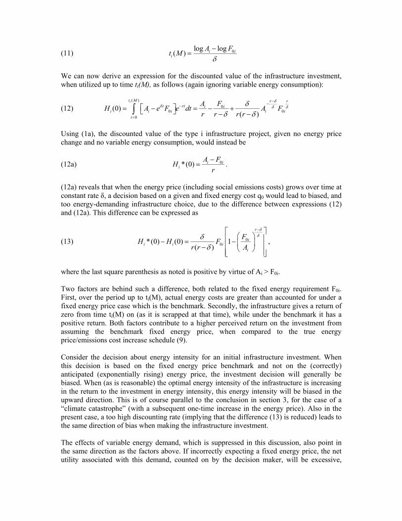
(11) 0log log( ) i i

i

A Ft M

We can now derive an expression for the discounted value of the infrastructure investment, when utilized up to time ti(M), as follows (again ignoring variable energy consumption):

(12) ( )

00 0

0

(0)( )

it M r rt rt i i

i i i i i

t

A FH A e F e dt A F

r r r r

Using (1a), the discounted value of the type i infrastructure project, given no energy price change and no variable energy consumption, would instead be

(12a) 0*(0) i ii

A FH

r

.

(12a) reveals that when the energy price (including social emissions costs) grows over time at constant rate δ, a decision based on a given and fixed energy cost q0 would lead to biased, and too energy-demanding infrastructure choice, due to the difference between expressions (12) and (12a). This difference can be expressed as

(13) 00*(0) (0) 1

( )

r

ii i i

i

FH H F

r r A

,

where the last square parenthesis as noted is positive by virtue of Ai > F0i. Two factors are behind such a difference, both related to the fixed energy requirement F0i. First, over the period up to ti(M), actual energy costs are greater than accounted for under a fixed energy price case which is the benchmark. Secondly, the infrastructure gives a return of zero from time ti(M) on (as it is scrapped at that time), while under the benchmark it has a positive return. Both factors contribute to a higher perceived return on the investment from assuming the benchmark fixed energy price, when compared to the true energy price/emissions cost increase schedule (9). Consider the decision about energy intensity for an initial infrastructure investment. When this decision is based on the fixed energy price benchmark and not on the (correctly) anticipated (exponentially rising) energy price, the investment decision will generally be biased. When (as is reasonable) the optimal energy intensity of the infrastructure is increasing in the return to the investment in energy intensity, this energy intensity will be biased in the upward direction. This is of course parallel to the conclusion in section 3, for the case of a “climate catastrophe” (with a subsequent one-time increase in the energy price). Also in the present case, a too high discounting rate (implying that the difference (13) is reduced) leads to the same direction of bias when making the infrastructure investment. The effects of variable energy demand, which is suppressed in this discussion, also point in the same direction as the factors above. If incorrectly expecting a fixed energy price, the net utility associated with this demand, counted on by the decision maker, will be excessive,

perhaps dramatically so, and will contribute to making the initial infrastructure excessively energy intensive.

5. Extension to positive shutdown risk Consider an extension of this model to a case with an exogenous risk of project “shutdown” (in which case the infrastructure loses its value), where this occurs with continuous flow probability μ (so that the time until shutdown is exponentially distributed with parameter μ). Technically speaking in the model, the effective interest rate now is r+μ instead of r. The corresponding expression for the value of the project can be written as

(14) 1

00(0)

( )( )

r ri i

i i i

A FH A F

r r r r

Here, all terms containing r are modified to instead contain r + μ. A question is how the possibility of project shutdown affects overall profitability and ranking of projects. We find, in particular, that the effect of a change in the rate μ at which project obsolescence occurs, on the value of a project of type i at the time of investment, is given by (15)

0 0 0 0 0 0

2 2 2 2

(0) [2( ) ]log

( )( )( ) ( ) ( ) ( )

r r

i i i i i i i i

i i i

dH A F r F F F F F

d A r r A Ar r r r

Here, all terms are negative except for the second, positive, term. The last three terms together represent changes in future energy costs due to an expected shortening of the project (physical) lifetime, when (economic) lifetime is at the same time capped by the condition that gross returns be non-negative. We find that dHi(0)/dμ has a generally ambiguous sign. An increase in the “scrapping rate” of the infrastructure investment (or alternatively, a shortening of its expected lifetime) reduces its expected value for a given constant fuel price (represented by the first term on the right-hand side of (15)). On the other hand, an increased scrapping rate reduces a potential loss associated with emissions later in the operation period for the infrastructure, which are subject to gradually higher energy cost, although only up to a limit given by the option to abandon the infrastructure (occurring at very high energy costs). We see however that when δ is small, there is a clear conclusion as the first term in (15) dominates over the second term and dHi(0)/dμ is always negative. When δ is larger (but less than r), the second term in (15) could dominate over the first term. Note here that while physical lifetime is stochastic (it is, under the current formulation, exponentially distributed up to maximum economic lifetime), economic lifetime is in this formulation deterministic and given solely by the (certain and known) energy price path (14).

6. Uncertainty about future fuel prices Uncertainty has so far played no role except with regard to the occurrence of a climate catastrophe (in section 3), and infrastructure obsolescence (in section 4), which both have

been assumed to be (Poisson process generated) stochastic events. We will here consider one rather modest extension of this framework to the case where the fuel price is simply stochastic, varying randomly around a particular value. We are here interested in studying how (long-run) average emissions may be affected by such uncertainty (represented by the variance on the stochastic price). Note first that this is an unrealistic way to represent uncertainty about the time path fuel and emissions price. It would instead be more realistic to assume that the price follows a stochastic process more directly in terms of its movements over time. Such a case (where the fuel price follows a geometric Brownian motion process with positive drift) is dealt with in Framstad and Strand (2010). We here let Eq denote the expected fuel price, and var q its variance. As before, we consider the two parametric, quadratic and log-linear, cases for utility of variable energy consumption. With quadratic utility results are relatively simple. First, since ex post energy consumption is linear in price in this case, from (2), uncertainty, and increases in uncertainty (in the sense of increasing the variance for given expectation), will leave expected energy consumption unaltered. A second issue is how expected utilities are affected by uncertainty. Note then that we have assumed basic risk neutrality (utility is linear in income). Expected utility resulting from the services rendered by this particular infrastructure, is under a quadratic utility specification affected in the following simple way

(16) 2

0

( ) var1, 1, 2

2i

i i ii

b Eq qEW A EqF i

c

.

In this case, the ex ante expectation of the variable part of utility (stemming from ex post variable energy consumption) now increases linearly in the variance of the fuel price. This is related to the optimization that takes place, with optimal adjustments in the short run to fuel price changes. Note that with c1 < c2 (as may be reasonable), a more variable fuel price increases EW1 by more than EW2, and thus by more in the high-carbon society than in its low-carbon counterpart. This is because there is more in absolute terms to gain by short-run adaptation of fuel demand, when demand is greater at the outset.21 These results are independent of the shape of the actual probability distribution. Thus, expected energy consumption depends only on the expected price; while utility depends on both expectation and variance of the price. Consider instead the log-linear utility function for short-term energy use, (1a). In this case the shape of the distribution function turns out to matter for results. Consider the simplest possible case, with a uniform distribution on a closed domain [q0-θ, q0+θ]. The range of this distribution is 2θ, with expectation q0 and variance θ2/3. Expected energy consumption is

21 This argument need not always apply, in particular not when infrastructure capital and energy input are “strong complements” as could e g be the case for the normal operation of a coal-fired power plant where the ratio between output and energy input is roughly fixed. Then there may be little to gain by variations in energy prices (except for extreme variations where a behavioural response is to shut the plant down). On the other hand, Strand and Miller (2010) have shown that the possibilities of retrofit of such a plant (possibly, with carbon capture and storage technology) may open up for substantial ex post substitutability which will in turn lead to a high ex ante value of energy price variations as indicated here; see the discussion below.

(17) 0

0

0

01

log1

2 2

iq

ii

q

q

qEF dq

q

.

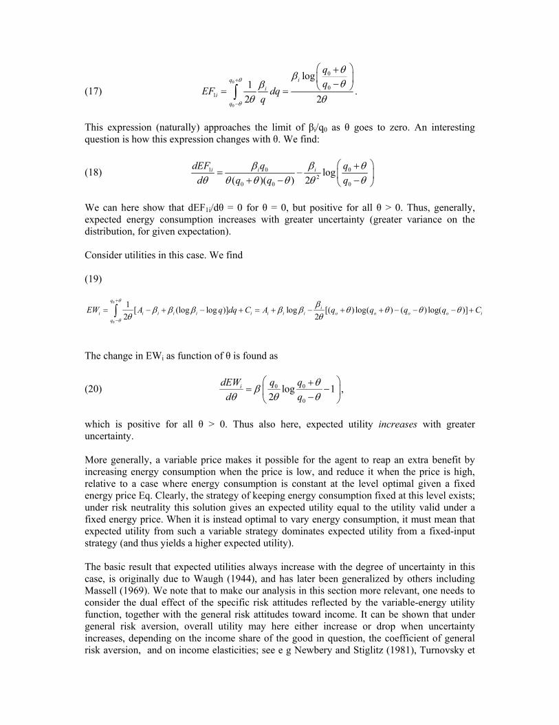
This expression (naturally) approaches the limit of βi/q0 as θ goes to zero. An interesting question is how this expression changes with θ. We find:

(18) 1 0 02

0 0 0

log( )( ) 2

i i idEF q q

d q q q

We can here show that dEF1i/dθ = 0 for θ = 0, but positive for all θ > 0. Thus, generally, expected energy consumption increases with greater uncertainty (greater variance on the distribution, for given expectation). Consider utilities in this case. We find (19)

0

0

1[ (log log )] log [( ) log( ) ( ) log( )]

2 2

q

ii i i i i i i i i o o o o i

q

EW A q dq C A q q q q C

The change in EWi as function of θ is found as

(20) 0 0

0

log 12

idEW q q

d q

,

which is positive for all θ > 0. Thus also here, expected utility increases with greater uncertainty. More generally, a variable price makes it possible for the agent to reap an extra benefit by increasing energy consumption when the price is low, and reduce it when the price is high, relative to a case where energy consumption is constant at the level optimal given a fixed energy price Eq. Clearly, the strategy of keeping energy consumption fixed at this level exists; under risk neutrality this solution gives an expected utility equal to the utility valid under a fixed energy price. When it is instead optimal to vary energy consumption, it must mean that expected utility from such a variable strategy dominates expected utility from a fixed-input strategy (and thus yields a higher expected utility). The basic result that expected utilities always increase with the degree of uncertainty in this case, is originally due to Waugh (1944), and has later been generalized by others including Massell (1969). We note that to make our analysis in this section more relevant, one needs to consider the dual effect of the specific risk attitudes reflected by the variable-energy utility function, together with the general risk attitudes toward income. It can be shown that under general risk aversion, overall utility may here either increase or drop when uncertainty increases, depending on the income share of the good in question, the coefficient of general risk aversion, and on income elasticities; see e g Newbery and Stiglitz (1981), Turnovsky et

al (1980), Gilbert (1993), and Federico et al (2001). The case for general risk aversion to be important is here underscored by the fact that the energy price relevant for the infrastructure investments is highly correlated with any general climate-related cost which affects a much wider range of commodities. In addition to “normal” ex post substitution possibilities, two further factors enhance the advantage of ex post variability of energy (including environmental) costs, as analyzed by Strand and Miller (2010). These are, first, the option to “retrofit” the energy technology; and secondly, the option to close it down; see also the discussion in the next section. The most important message to take home from this section is that greater uncertainty about the future energy price will, quite generally, make it attractive to invest in more energy-intensive infrastructure if such investment does not preclude ex post variation in energy utilization as prices change. This follows here quite directly as high (potential) energy intensity becomes more profitable when more opportunities arise to exploit low energy prices (which will arise with higher variance on these prices). But it also follows for other reasons, when additional options (to retrofit and/or close down the infrastructure) are added to the story.

7. The Retrofit Option A natural extension to the basic model implies the possibility of “retrofit”, whereby part or all of the (fossil) energy requirement can be removed from the infrastructure, while the infrastructure is otherwise operated as normal. Since this is a main topic of Framstad and Strand (2010), and Strand and Miller (2010), we will not go in analytical detail on this issue, but only discuss some principal points. A “retrofit option” can be thought of in at least two ways. One is that fossil energy is replaced by non-fossil energy in operating the infrastructure. The other way is to retain fossil energy, but to remove the resulting carbon emissions through sequestration (carbon capture and storage, CCS). Quite generally and almost trivially, the retrofit option will be applied when it reduces the cost for the decision maker, relative to a relevant alternative (infrastructure operation as usual; or infrastructure closedown). Analysis of a retrofit option is most straightforward in a situation with no uncertainty, or where all uncertainty is resolved at one particular time as in the case of a climate catastrophe in section 3 (which includes uncertainty about the retrofit cost itself), in which ordinary decision criteria (for whether and when to implement the retrofit) apply. The availability of retrofit as an option has at least three major consequences for the infrastructure decision and its implications. First, the “fixed” (fossil) energy demand of the infrastructure is no longer fixed but may be avoided in cases where this is economic advantageous. This leads to a lower ex ante expected energy cost associated with the infrastructure, at the time of basic investment, for any given energy intensity chosen. Secondly, availability of a retrofit option leads to lower total (energy, plus retrofit) costs, relative to energy costs only in the case of no retrofit option, for a given initial energy intensity chosen. The overall average cost saving is greater when energy and retrofit costs are both more variable, and when the two cost components are less (or negatively) correlated.

The third, and related, issue to note is that since expected energy cost is reduced, it is optimal (for the decision maker) to choose a more energy-intensive infrastructure type at the time of investment. This factor may (partly or fully) eliminate the tendency for energy saving that follows from the retrofit option being exercised. It is here possible to find (reasonable) specifications of the function defining the utility of an infrastructure investment with given cost as a function of its energy intensity, which lead to an overall energy cost increase when expected unit energy costs are reduced; although this is not the typical case.22 Under more general uncertainty (in particular, about the future energy price path), such as when the marginal cost of additional GHG emissions drifts upward but with a random component, the situation is more complex. The retrofit option is likely to take a “lumpy” form (requiring a discrete investment to be sunk), which implies, under continuous uncertainty, a positive option value associated with waiting to exercise the retrofit. This is studied in more detail in Framstad and Strand (2010).23 The retrofit decision is as a consequence delayed, relative to the situation with a deterministic energy cost path. In turn, the initial infrastructure investment is made less energy intensive. Note that this uncertainty, and resulting delay, leads to greater expected energy consumption, the welfare effect of the uncertainty is positive (at least in the case of a risk neutral decision maker), for well-known reasons (namely, that uncertainty opens up for more cost avoidance in particularly unfavorable states; and the bearing of more costs in particularly favorable states). Overall, the availability of a retrofit option tends to “soften” the otherwise rather rigid relationship between the initial investment and later fossil energy consumption and thus carbon emissions; and in particular reduces the risks associated with particularly high future energy and emissions prices. This “softening” at the same time leads to more “risky” behavior in the sense that initially chosen emissions intensities are higher. When attempting to apply this line of argument to actual infrastructure investments, the actual scope for retrofit is crucial. For some technologies such as CCS as applied to individual power plants, or perhaps more general electricity generation based on newly developed renewable sources, ex post retrofit seems highly relevant and may, potentially, avoid almost all the fossil-fuel consumption and/or carbon emissions associated with the initial infrastructure. In other cases, such as for retrofitting general urban structures, this scope may be less. In any case, the possibility of new future energy technologies is likely to represent most of the source of such uncertainty; and should thus be greatly stimulated.

8. Conclusions The main conclusion from the above discussion is that long lasting and energy demanding (or committing) infrastructure investments, that tie up energy consumption at high rates for long future periods, likely tend often to be too energy intensive. This is tied to several factors, some of the most important of which are these:

22 In particular, given that the utility function belongs to the class of CRRA (constant relative risk aversion) functions, initial energy demand will “overreact” to an expected future cost reduction (thus increasing expected ex ante energy costs) if and only if the utility function takes the Cobb-Douglas form. When the utility function instead is logarithmic (another CRRA specification; which is exemplified above in this paper), the ex ante increases in energy demand and reductions in unit energy cost are exactly counterbalanced, and overall expected energy costs remain fixed. 23 See also Strand (2009) for a related model of “mitigating retrofits” when background uncertainty is altered.

1. The energy/emissions price on which investment decisions are based, tend to be lower

than the “correct” prices (which would embed a social marginal cost of GHG emissions, which is typically not embedded).

2. Since energy/emissions prices will, most likely, tend to increase over time, this entire

future increasing price path ought in principle to be considered in sinking the investments; but much if not most infrastructure investment has (explicitly or implicitly) a shorter-time and/or more myopic perspective.

3. Related to the two foregoing two points is that the (explicit or implicit) rate of

discount used for infrastructure decisions, is usually higher than the appropriate rate of interest for discounting future climate damages. This tends to put too much emphasis on periods close up in time, when energy/climate costs are low.

4. There may be a tendency to underestimate the possibility of very severe climate

events, that are objectively likely but that have not yet occurred and whose likelihood may as a result be undervalued.

Overall, these prospective biases imply that great care must be taken in handling, and affecting, the process of energy-intensive and -committing infrastructure investment. Such investments are made only infrequently but with great impact when actually made. Once the investments have been made, it can be very difficult and costly to reduce substantially the carbon emissions level that is “naturally” tied to operating the infrastructure. Such care in weighing long-lived investment options carries over to the formulation of national development plans supported by international financial institutions and other international partners.

Appendix: Infrastructure choice with Cobb-Douglas utility Consider now a very simple case where the utility function of the representative consumer is given a Cobb-Douglas specification, implying that the social objective function over two periods takes the following form: (A1) 1 ( ), 1, 2t t t t tW C F Y C q F t

The premise here is that energy consumption in either of the two periods, F, stays constant at least within each period (as when F represents variable energy demand), and possibly across the two periods (when F represents the fixed energy demand of the chosen infrastructure). The second period can here be longer than the first (length represented by a relative coefficient T ≥ 1); this is taken to represent a situation where F is tied to infrastructure established in period 1. Once infrastructure investments have been made, F can in this case no longer be changed. We however assume that F can be set freely at the start of period 1. Consumption of the “other”, generic, good, C, can in principle change between periods. Incomes in the periods, Yt, are assumed to be exogenous but can vary. Assume also that the consumer/society can borrow and lend freely at interest rate r, with corresponding discount factor δ = 1/(1+r). A key assumption is q2 > q1: the price of energy increases over time; while the price of the generic good C stays constant (or is numeraire). We abstract from initial investment costs in period 1, which may be taken to be identical between different energy-intensity alternatives.

Maximizing W1 + W2 with respect to F and the Ci in this case yields, for the case of fixed energy demand associated with the infrastructure:

(A2) 1 2

(1 ),

av

YF C C Y

q

where qav = (q1+δTq2)/(1+δT) is the average energy price over the horizon, while the price of C is normalized to unity. Y is in a simplest case constant over time.24 In the case where F represents short-run energy demand, the demand function valid for period t would rather be

(A3) 1 2

(1 ),t

t

YF C C Y

q

The Cobb-Douglas formulation leads to particularly simple demand functions, as budget shares for the two goods, over the lifetime for the infrastructure (qavF for fuel, and C for rest consumption) in this case turn out to be constant fractions (1-α, and α respectively) of total income. This consequently represents a different and opposite “extreme” case to that under the first two models, where variations in total income now forces a proportional variation in (infrastructure-based) energy demand (in previous cases, remember, the extreme was no income effect on energy demand whatsoever). When comparing the current case to (2a), with a log-linear utility function in energy consumption in section 2 above, note that in both cases energy demand is inversely proportional to the energy price. The energy intensity is in this case chosen based on the (discounted) average energy price over the lifetime of the infrastructure investment. This is a very simple and intuitive decision rule, and easy to interpret. Given this rule, any inefficiency in the decision process is essentially tied to the average energy price pav. When this price is “too low”, F is socially excessive and too much is invested initially in productive capacity to allow future energy consumption. As above this price can be low for a variety of reasons, some of which are due to pricing and others due to efficiency issues.

The CES formulation To remedy some weaknesses of the model formulations above, one may instead introduce a CES utility function with two goods groups (generic goods; and energy goods) specified. The CES can be viewed as a generalization of the Cobb-Douglas utility function to the case of arbitrary non-negative substitution elasticity (which is unity in the Cobb-Douglas case). More generally with the CES, budget shares will be variable. The shares for energy goods will vary positively (negatively) with the energy price when the substitution elasticity is less (greater) than unity. Using a nested CES function, utility is given by the following expression: 24 Alternatively, if Y varies, Y in (A2) would need to be replaced by Yav = average per-period income over the relevant horizon.

(A4) 1

( , ) (1 )U C F C F

where F is a generalized fuel input function (which could represent a composite of different fuels Fi, i = 1, .., n), given by

(A5)

1

1

n

i ii

F F

.

In the simplest case, with n = 1, we would have γ1 = 1. We have two composite goods, “C”, and n different types of fuels Fi which are substitutable. We now simplify by assuming that fuel demand is generally variable. Given this we obtain the following demand functions for each type of fuel:

(A6) r

ri i

i

pF F

p

.

Here we have defined:

(A7) rn

i

ri

ri pp

1

1

1

1~ ,

pi is the price of each fuel i, and we have defined

1

1r . The aggregate demand for fuel

and the “other” good are given by:

(A8) 11 s

YC

p q

, 11

s

s

p qF Y

p q

,

where Y is consumer income, and where

(A9) s

q

1

,

We have here normalized the price of the composite good to unity. r and s are elasticitities of substitution, between fuels, and between the composite fuel and the other composite good, respectively.

References:

Dasgupta, Partha S. and Heal, Geoffrey M. (1979), Economic Theory and Exhaustible Resources. Cambridge: Cambridge University Press. Federico, Giulio; Daniel, James A.; and Bingham, Benedict (2001), Domestic Petroleum Price Smoothing in Developing and Transition Countries. MIF Working Paper, no 01/75. Washington DC:International Monetary Fund. Framstad, Nils Christian and Strand, Jon (2010), Inertia in infrastructure investment with “retrofit”: A continuous-time option value approach. Forthcoming paper, World Bank. Gilbert, Christopher L. (1993), Domestic Price Stabilization Schemes for Developing Countries. In S. Claessens and R. C. Duncan (eds.): Managing Commodity Price Risk in Developing Countries. .Baltimore: Johns Hopkins Press. Hotelling, Harold (1931), The Economics of Exhaustible Resources. Journal of Political Economy, 39(1): 137-175. Jaccard, M. (1997), Heterogeneous Capital Stock and Decarbonating the Atmosphere. Does Delay make Cents? Working Paper, Simon Fraser University. Jaccard, M. and Rivers, N. (2007), Heterogeneous Captal Stocks and the Optimal Timing for CO2 Abatement. Resource and Energy Economics, 29, 1-16. Leibowitz, S. and Margulis, S. (1995), Path Dependency, Lock-In and History. Journal of Law, Economics and Organization, 11, 205-226. Massell, Benton F. (1969), Price Stabilization and Welfare. Quarterly Journal of Economics, 83, 284-298. Newbery, David G. and Stiglitz, Joseph E. (1981), The Theory of Commodity Price Stabilization. Oxford: Clarendon Press. Shalizi, Zmarak and Lecocq, Franck (2009), Economics of Targeted Mitigation Programs in Sectors with Long-Lived Capital Stock. Background paper for the World Development Report 2010. Stern, Nicolas et al (2007), The Stern Review: The Economics of Climate Change: London: Her Majesty’s Treasury. Strand, Jon (2009), Implications of Dampened Uncertainty in a Continuous Stochastic Model of Mitigation. Unpublished, the World Bank. Strand, Jon and Miller, Sebastian (2010), Climate Cost Uncertainty, Retrofit Cost Uncertainty, and Infrastructure Closedown: A Framework for Analysis. Policy Research Working Paper 5208, the World Bank.

Turnovsky, Stephen J.; Shalit, Haim; and Schmitz, Andrew (1980), Consumer’s Surplus, Price Instability, and Consumer Welfare. Econometrica, 48, 135-152. U.S. Department of Energy (2007), Scenarios of Greenhouse Gas Emissions and Atmospheric Concentrations. U.S. Climate Change Science Program, Synethesis and Assessment Product 2.1a. Washington DC: U.S. Department of Energy. Waugh, Frederick V. (1944), Does the Consumer Benefit from Price Instability? Quarterly Journal of Economics, 58, 602-614. World Bank (2009), World Development Report 2010: Development and Climate Change. Washington DC: The World Bank.