Inequalities and Identities

Sanjay G. Reddy∗ and Arjun Jayadev+

November 23rd, 2011

Abstract We introduce concepts and measures relating to inequality between identity groups. We define and discuss the concepts of Representational Inequality, Sequence Inequality and Group Inequality Comparison. Representational Inequality captures the extent to which an attribute is shared between members of distinct groups. Sequence Inequality captures the extent to which groups are ordered hierarchically. Group Inequality Comparison captures the extent of differences between groups-. The concepts have application in interpreting segregation, clustering and polarization in societies. There exists a mapping from familiar inequality measures to the measures we identify, making them empirically applicable.

∗ New School for Social Research ,Economics Department.and School of International and Public Affairs, Columbia University, reddys1@newschool.edu + Economics Department, University of Massachusetts, Boston arjun.jayadev@umb.edu

1

"Civil paths to peace also demand the removal of gross economic inequalities, socialhumiliations and political disenfranchisement, which can contribute to generatingconfrontationandhostility.Purelyeconomicmeasuresof inequalitydonotbringout thesocialdimensionof the inequality involved.Forexample,when thepeople in thebottomgroups in terms of income have different non‐economic characteristics, in terms of race(such as being black rather than white), or immigration status (such as being recentarrivals rather than older residents), then the significance of the economic inequality issubstantiallymagnified by its "coupling"with other divisions, linkedwith non‐economicidentitygroups."AmartyaSen,TheGuardian,FridayNovember9th,2007 Introduction Do differences in the economic and social achievements of distinct groups merit attention? Sen’s remarks above suggest that the salience of interpersonal differences in welfare can be increased when these are correlated with certain other differences among individuals. Such a conclusion can be justified from at least two perspectives. First, inter-group differences may possess an intrinsic significance from the standpoint of assessments of justice and fairness in the distribution of goods and opportunities.1 Second, the fact that there exist distinct groups in society and that these groups exhibit inter-group differences may have instrumental significance from the standpoint of their impact on social goods such as peace, stability or economic growth. The concern with the intrinsic significance of inter-group differences has centered on the degree to which ‘morally irrelevant’ characteristics of a person (such as belonging to a given race, sex, caste or other group as a result of birth) should be permitted to determine her or his life chances2. Such a motivation is distinct from one based on the idea that social goods or ‘bads’ may be generated by inter-group differences in economic and social achievements, and that inter-group differences may be relevant for that reason. A long standing body of literature in economics and other social sciences has empirically explored this instrumental concern.3 Both concerns have led to the development of a growing literature which has identified and empirically examined such concepts as ‘horizontal inequality’, segregation, polarization and related ideas about differences between groups. That a multitude of concepts concerning inter-group difference has been proposed is not entirely surprising in light of the fact that such differences can be understood as occurring in more than one way. For example, studies on segregation focus on the degree to which members of different groups share a location, occupation or other attribute while studies on horizontal inequality focus 1 See Appendix One for a brief discussion. 2 For a review of these debates, see e.g. Roemer (1996) and Sen (1992). Arguments that societies should be organized so as to limit the consequences of the “brute luck” of being born into a particular position include those of “luck egalitarians” such as Arneson (1989), Cohen (1989), Dworkin (2000), Rawls (1971) and Roemer (1996). Egalitarians of other kinds may come to similar conclusions for different reasons (see e.g. Anderson (1999)). 3 For some recent examples see e.g. Stewart (2001), Alesina et al (2003), Alesina and La Ferrara (2000, 2002), Montalvo and Reynal Querol (2005), Miguel and Gugerty (2005) and Østby (2008).

2

on the extent of difference in the income or other achievements of separate groups. In both cases however, the subject of interest is the degree of unevenness or inequality in the possession of attributes between groups. The goal of our paper is to elucidate some distinct ways in which inter-group differences can be conceived, which encompass but are not restricted to the concerns of these existing approaches. A common underlying concern in analyses of inter-group differences is the degree to which distinct groups are systematically over-or under-represented in their possession of various attributes (levels of income or health, club membership or political office etc.). In this paper we introduce the concept of Representational Inequality (RI) as a way to capture this concern. This concept describes the extent to which a given attribute (for instance, a level of income or health, or right or left handedness) is shared by members of distinct groups. It can be used to measure the degree of ‘segregation’ of distinct identity groups in the attribute space.4 When individuals can be ordinally ranked in relation to an attribute (such as income or health but not right or left handedness) we may be interested not only in how segregated or separated each identity group is in terms of their achievements, but in some measure of their relative positions in the ranking. Sequence Inequality (SI), understood as the degree to which members of one group are placed higher in a given hierarchy than those from another, captures this concern. Such a concept provides an intuitive framework for understanding the degree of ‘clustering’ of various identity groups in distinct sections of a hierarchy.5 When individuals’ level of achievement can also be cardinally identified for an attribute (as for income but not for right or left handedness) the distance between groups’ attribute levels may be of interest. We may identify a distinction between two different concepts, which we term respectively Group Inequality Comparison (I) and Group Inequality Comparison (II) and abbreviate as GIC (I) and GIC (II). The concept of Group Inequality Comparison (I) involves a comparison of counterfactuals. Specifically, it is derived by comparing the inequality arising in a society in which all of the members of a group are assigned a representative income for that group and the total interpersonal inequality in a society. This concept is concerned with identifying the extent to which between-group inequality ‘accounts for’ overall inequality in society. Group Inequality Comparison (II) by contrast measures only the inequality arising in the first situation, i.e. that in a society in which all of the members of a group are assigned a representative income for that group. This latter concept is concerned with the absolute magnitude of the inequality generated by between-group inequality. Our purpose in this paper is two-fold. We seek not only to clarify the concepts described above but to show that combining them can provide a way to understand conjoint concepts of group differences. In particular, ‘polarization’,6 understood to involve the collection of like elements and the separation of such collections of like elements from one another, can be fruitfully 4 Segregation is defined by the Oxford English Dictionary, inter alia, as “The separation of a portion of portions of a collective or complex unity from the rest; the isolation of particular constituents of a compound or mixture”. 5 A cluster is defined by the Oxford English Dictionary as, inter alia, “A collection of things of the same kind…growing closely together; a bunch… a number of persons, animals, or things gathered or situated close together; an assemblage, group, swarm, crowd.” 6 The Oxford English Dictionary defines the verb “polarize” as “To accentuate a division within (a group, system, etc.); to separate into two (or occas. several) opposing groups, extremes of opinion, etc.”

3

described as involving the simultaneous presence of between-group differences of different kinds. The combination of Representational Inequality with Sequence Inequality alone provides a measure of what might be termed ‘Ordinal Polarization.’ Combining Group Inequality Comparison (of either type I or type II) with these other two indices can provide a richer index of Polarization applicable to the case in which the attribute is cardinally measurable as well. Our purpose is not to provide a unique characterization of a single measure of polarization, but rather to show that a broad class of measures of polarization can be derived from a simple set of unexceptionable axioms concerning different types of between-group differences and their combination. The concept of polarization that we employ here is distinct from that developed in the preponderance of the existing literature in that it draws on information about the identity groups to which those who possess distinct attributes belong. In contrast, the existing frameworks generally employ a ‘collapsed’ framework in which the level of the attribute (typically income) defines the identity group (Esteban and Ray (1994), Duclos, Esteban and Ray (2004)). In these frameworks, polarization of an income distribution is understood to involve ‘identification’ between individuals possessing a certain level of income and ‘alienation’ between those individuals and others possessing different incomes. In our framework, in contrast, polarization of an income distribution is understood to involve segregation of individuals belonging to distinct identity groups at certain levels of income and the separation of these groupings of individuals in the income space from other groupings of individuals possessing distinct identities. Part I: Concepts of Group Inequality One approach to evaluating inter-group differences is to construct a measure of overall group advantage or disadvantage for each group prior to assessing the differences in these overall measures.7 Although there can be advantages to such an approach, it can obscure the diverse aspects of inter-group difference (by reducing inter-group differences to inequalities in a single dimension). We accordingly explicitly identify here three distinct concepts of inter-group difference, and a fourth which builds upon them. Representational Inequality: We define a situation of representational inequality as occurring when, for some attribute and some identity group, the proportion of the group possessing the attribute is either greater or less than the proportion of the group in the overall population. To provide some graphical intuition for this idea, consider the distribution of income among different groups in a society that consists of fifty percent whites and fifty percent blacks. Figure 1 depicts the situation in which there is no representational inequality. The location of each bar on the horizontal axis represents an income level ordered from lowest to highest and the proportion of persons possessing that income of either group is represented through shading. At all levels of income, blacks and whites are 7 See Jayaraj and Subramanian (2006) for an example of such an approach.

4

represented in equal proportion to their share of the population as a whole (i.e. one half each). Any deviation from such equi-proportionality leads to a situation of representational inequality. Such a situation is depicted in Figure 2, in which at certain levels of income blacks or whites comprise a larger or smaller proportion of the individuals possessing that level of income than they do in the population as a whole. While the situation depicted in Figure 2 is one of representational inequality, both groups are represented at all the incomes. In contrast, Figure 3 depicts a situation in which at each level of income there is complete segregation, in the sense that at each level of income there is one and only one identity group represented. It may be noted that although this is a situation of complete segregation the incomes at which whites and blacks appear are evenly interspersed. We depict this example in order to make sharp the distinction between segregation and clustering as we use the terms. The former refers to a situation in which those possessing a specific attribute (in this case an income level) belong disproportionately to a particular group. The latter refers to a situation in which the attributes disproportionately possessed by members of a particular group are grouped together in a certain part of an attribute hierarchy (in this case the income spectrum). The concept of representational inequality clearly need not be restricted to a scenario in which the attribute is cardinally orderable. Thus, for example, we can apply the principle in an equally straightforward manner to unordered attributes such as location of residence, or membership in distinct clubs or legislatures. If instead of income brackets, each bar referred to a distinct legislature in a federal country, the figures we have discussed here would depict the degree of inequality in political representation. Sequence Inequality The distinction between ‘complete segregation’ and ‘complete clustering’ can be seen by comparing Figure 3 and Figure 4. Figure 4 depicts the situation that results from a transfer of incomes such that all the whites move to the richer half of society while all the blacks move to the poorer half of society. This situation is one in which each sub-group is concentrated in a different part of the income distribution. Such a situation can plausibly be described as one of ‘complete clustering’ of groups8. In both cases, there is complete segregation and thus maximal representational inequality. However, in Figure 3, whether an individual is black or white provides very little information on his or her rank in society. By contrast, in Figure 4, whether an individual is black or white provides a great deal of information. One simple way to capture the distinction between Figure 3 and Figure 4 is through the concept of sequence inequality, which together with representational inequality captures the clustering of the income distribution. This concept is linked to the position in the overall societal ranking possessed by individuals belonging to distinct groups in the hierarchy. An individual (weakly) rank-dominates another if that individual is ranked equal to or higher than the other in the possession of the attribute. For any population partitioned into given identity groups, there are a fixed number of between-group pair-wise comparisons between individuals from different identity groups. The share of the total number of such between group pair-wise 8 Massey and Denton (1988) make reference to equivalent concepts

5

comparisons involving a given group in which a member of the group rank-dominates a member of some other group is called its level of group rank dominance. Group rank dominance is an indicator of the position the group occupies in the ordinal hierarchy of attribute levels. Another way to understand the difference between Figure 3 and Figure 4 is simply that the average rank of the whites and the blacks is different. This is clearly a necessary condition for distinct groups to be clustered in different parts of the attribute space. We establish in Appendix Two that a monotonic relationship exists between the concepts of group rank dominance and of average rank. Both of these could be seen to be indicators of the placement of groups in the attribute hierarchy (in the extreme complete clustering of groups) and will thus be referred to as indicators of a group’s rank sequence position. The level of inequality in different groups’ rank sequence position (whether as measured by group rank dominance or by average rank) indicates the extent to which a population is clustered. We refer to this concept of inequality as sequence inequality (SI). Some reflection will suffice to show that this is an unambiguous criterion even when group sizes differ. In any situation sequence inequality is minimal when the groups are evenly interspersed or symmetrically placed around the median member(s). It is clear from this discussion that while Figure 3 and Figure 4 depict two groups with equal representational inequality, the two groups possess different levels of group rank dominance and average rank. In Figure 4, whites have 100% of the available instances of rank domination and higher average rank. While sequence inequality and representational inequality are related, they are also distinct concepts. A simple example which makes this distinction transparent is provided in Figures 5 and 6. In Figure 5, both groups possess the same level of group rank dominance and average rank. The black group has two of the possible four instances of rank domination as does the white group, and their average rank is the same. Thus there is no sequence inequality between the groups. In the second, both groups again share equally in levels of group rank domination (both have two of the potential four instances once again) and have the same average rank. The situation once again is one in which there is no sequence inequality. However, in the first case there is complete representational inequality and in the second case there is zero representational inequality. In neither case is group membership always associated with higher rank, yet the cases differ in the degree to which income levels are shared by members of distinct groups. Group Inequality Comparison Figure 4 depicts a situation of maximal representational inequality and maximal sequence inequality. It could perhaps be thought of as a situation of polarization in the sense that each group is concentrated at a given pole of the income distribution. However, this is true only in an ordinal sense. Both the situations depicted in Figure 4 and in Figure 7 are identical from the standpoints of representational inequality and sequence inequality since neither concept takes note of cardinal information, which alone accounts for the difference between the two situations described. To take account of cardinal information (for instance, concerning the distance between distinct clusters), it is necessary to introduce an additional concept.

6

A common way to account for such information is to take note of the distance between the means of distinct sub-populations, for example by using measures of inequality between group means. This, indeed is the conception behind Group Inequality Comparison (II). However such an approach ignores relevant information on within group inequality. Consider a two-group society in which all members of each group originally respectively possess the mean incomes of their groups. Suppose that both groups experience within-group transfers leading to intra-group inequality. The extent of inequality in the society must be judged to have increased if the measure of inequality employed obeys the Pigou-Dalton Transfer Principle (ensuring that such transfers between persons are deemed to increase overall inequality). However, between-group inequality (understood in terms of inequality between mean incomes of groups) is unchanged. Between-group inequality must be deemed to have become relatively less substantial in comparison with total interpersonal inequality. An approach to inter-group inequalities which is based on between-group inequalities in isolation rather than on the contribution of between-group inequality to overall inter-personal inequality (i.e. Group Inequality Comparison (II)) will fail to contrast situations that might be distinguished. Consider Figure 8 which depicts a two group society in which all members of each group originally possess mean income A and B respectively. Both groups now experience within-group transfers which increase inequality and their distributions are now depicted by densities A’ and B’ respectively. Assume further that the transfers are such that the span between the means is Δ and the span between the richest and poorest members of each group is also Δ. We might plausibly consider inter-group differences to have become less significant after the transfer since no member of the richer group is further away from some member of the poorer group than before the transfer, and all but the very richest member of the richer group is closer to some member of the poorer group. On the other hand, Group Inequality Comparison (I) can have the disadvantage of ignoring information relevant for understanding the extent to which inter-group differences generate overall inequality. To see this, consider what would happen if in Figure 8, the original populations A and B were made arbitrarily closer to each other while maintaining their separation. According to Group Inequality Comparison (I), there would be no difference between the two situations. If we employed instead the concept of Group Inequality Comparison (I) the degree to which between group differences generate inequality will have fallen. It can be seen that there are potentially good reasons to choose wither approach. Group Inequality Comparison need not be measured, of course, in terms of differences in means and could potentially be understood in other ways -- for instance in terms of differences in medians, generalized means, or other measures of central tendency. Indeed, still other ways of viewing group differences can be envisioned, for example involving comparison of higher moments of the group-specific distributions of incomes, examination of the extent of ‘non-overlap’ between distributions etc. For a wide-ranging discussion of methods of defining group separation, see Anderson (2004, 2005). We limit our further discussions of the concept however to the case where it is measuring mean differences, for expositional simplicity.

7

Combining Concepts: Polarization We have introduced above three concepts relating to inter-group inequalities: representational inequality, sequence inequality and group inequality comparison. How are these concepts related to polarization? Polarization is a concept which has been used in many different ways in the literature, for example, to mean the absence of ‘middleness’ in a distribution (Wolfson, 1994), the distance between the average achievements of groups (Østby, 2008) and the presence of distinct sizable groupings in the income distribution (Esteban and Ray, 1994). Many of these approaches do not explicitly rely on the identification of individuals by identity groups (understood as being distinct from attributes). A contrasting approach understands the level of polarization of a distribution in terms of the extent of inter-group differences in the possession of an attribute. If polarization is defined in this way, it becomes clear that each one of the concepts of inter-group inequality defined above is itself a measure of polarization. However, taken individually each may prove to be an unsatisfactory measure of polarization, because of the information to which each is individually indifferent. Thus the relative ranking of the situations depicted in Figure 3, Figure 4 and Figure 7 according to the extent of polarization depends on the expansiveness of the approach used. In particular, all the figures depict maximal polarization as judged according to RI, whereas Figures 4 and 7 depict maximal polarization according to both RI and SI, and Figure 7 depicts a higher degree of polarization than does Figure 4 according to GIC (taking the figures to possess the same income scale on the horizontal axis). The fact that our judgments regarding the polarization of society may depend on more than one concept suggests the value of combining measures of inter-group differences to construct orderings of social situations according to the extent of their polarization. Such orderings can be partial and based on dominance of the vectors (2-tuples or 3-tuples) defined by the individual measures of inter-group differences, or can be complete if based on some method of aggregation of these measures. This said, orderings based on combining only a pair of the concepts we have defined (and not all three) will be indifferent to some important considerations that may be deemed relevant in any assessment of polarization. We have already seen that in the two group case, combining representational inequality and sequence inequality will be sufficient to give us a measure of ordinal polarization. Such a combination however will be indifferent to cardinality and will be unable to distinguish, for example, between the situations depicted in Figure 4 and Figure 8 respectively. A measure combining sequence inequality and group inequality comparison is not indifferent to cardinal information on the achievements of individuals but it is indifferent to the degree of clustering of identity groups in any specific income bracket. In order to see this, consider Figures 5 and 6 again. Let us assume that, by construction, the mean income of both blacks and whites is the same in both groups in both situations. If this is the case, the index of group inequality comparison is the same in both figures (i.e. zero) and sequence inequality is the same, but representational inequality is different. We may argue that in Figure 5 there is no clustering of identity groups in distinct parts of the income spectrum, as there is no representational inequality. In Figure 6, however, blacks are clustered at the top and bottom ends of the income spectrum, and indeed there is complete segregation between the two groups. Note further that we could

8

increase the distance between the blacks at the ends and the whites in the middle, keeping the means of both groups the same (so that the blacks at each end are very distant from the whites at the center) and yet record the same level of polarization defined according to such a measure. Finally, combining representational inequality and group inequality comparison (I) alone leads to an approach that is indifferent to the sequencing of individuals from distinct identity groups in the income spectrum. Consider the distinction between Figure 9a and Figure 9b. Both depict cases of complete segregation. However in Figure 9b, some population of blacks has been moved to a higher income than all of the whites, thereby increasing within group inequality for the blacks and total inter-personal inequality. We can further imagine that every white has been given a higher income in such a way that within-group inequality among whites is unchanged and the ratio of between-group inequality to total inequality (which would otherwise have fallen) is restored to its level prior to the initial movement of blacks. In other words, the index of group inequality comparison (I)remains the same by construction, as does representational inequality. However, the sequencing of blacks and whites in the income distribution (and thus sequence inequality) is different. An analogous argument can be made for group inequality comparison (II) by moving the blacks and whites so as to keep mean incomes of the groups the same. Any approach to polarization based on a pair of the group inequality concepts we have defined will capture certain judgments about social situations and neglect others. Only by combining all three concepts can an approach to polarization which takes account of the considerations reflected in each of the concepts be constructed. A variant of group inequality comparison (I) has been proposed as a stand-alone measure of polarization (Kanbur and Zhang, 2001). However, such a measure, while attractive in its simplicity can violate some intuitions. Consider Figure 10 in which two completely segregated and clustered groups A and B experience within-group progressive transfers which reduce within-group inequality. Further suppose that they also experience a reduction of between-group inequality through progressive transfers between the members of the two groups in such a way that the ratio of between-group inequality to overall inequality remain unchanged and the groups ( whose densities are now depicted by A’ and B’) overlap. If we utilize group inequality comparison (I) alone as our measure of polarization, a social configuration with A and B is viewed as being exactly as polarized as a situation with A’ and B’, which seems to conflict with our intuitions. If we, however, combine it with some measure of sequence inequality and /or representational inequality (both of which are lower when the groups overlap), the first situation is unambiguously more polarized than the second. It should be noted that the regressive transfers considered above led to a decrease in the index of group inequality comparison (I) and therefore their impact was in the opposite direction from that which would normally be expected of an inequality measure ( i.e. to obey the Pigou-Dalton principle of responding to a regressive transfer with an increase in measured inequality). It follows that any measure of polarization which increases when the index of group inequality comparison (I) increases would similarly potentially violate the Pigou-Dalton principle9.

9 This view corresponds to the findings of Esteban and Ray (1994) among others that polarization and inequality are distinct concepts and that measures of polarization need not therefore be expected to obey the Pigou-Dalton principle.

9

Part II: From Concepts to Measures Formalizing Concepts Our purpose in this section is to formalize the concepts relating to group differences which we have introduced above and develop measures of them10. We begin by supposing a `social configuration’ ( ) in which there is a population, S0, of individuals {i} of size N partitioned11 into K distinct identity groups (S1, S2....SK). The individuals possess an attribute (let us say y), drawn from an attribute set, Y. The attributes are not necessarily ordered. For example, the attribute may be a level of income (ordered and cardinally measured), a quality of health (ordered but not cardinally measured) or a club to which a person may belong (distinguished from one another, but not ordered). We employ a superscript to distinguish the information associated with distinct social configurations. For simplicity, we assume (although nothing depends on this other than notation) that the number of elements, l, in the set Y, is finite. More specifically, the individuals {i} each belong to a distinct identity group so that

, for some J , with

and .

Our assumptions imply there are at least two identity groups which are each smaller than the population as a whole and non-empty. Let the number of persons in group J be denoted by nJ. The proportion of persons of a group J in the society is defined by

for .

Each individual i has attribute . The same attribute may be shared by more than one individual. 10 These measures can be readily implemented using a Stata module that we have developed and which will be made publicly available in due course. For a ready example of how these measures can be and have been applied to actual data, see Reddy and Jayadev (2009). 11 We do not consider currently the case of societies in which individuals belong to more than one identity group simultaneously and in which the identity groups do not form a partition of the society into mutually exclusive categories. Generally, a partition of a society can be constructed on the basis of the Cartesian product of the identity groups in the society. This solution may not be deemed appropriate, however, in every situation. For example, a mixed race group in a society otherwise divided into two races may be deemed to belong to both of the races rather than to neither, and it may be thought that this characterization is relevant to our judgments regarding inter-group differences.

10

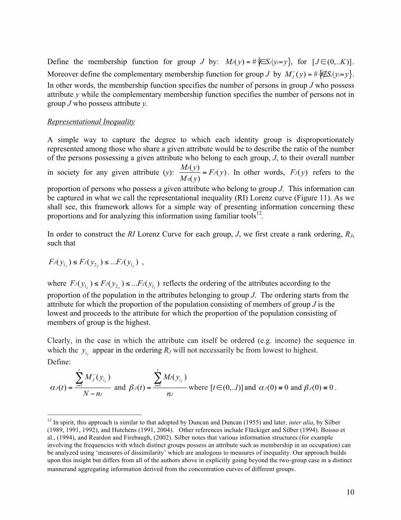
Define the membership function for group J by: , for . Moreover define the complementary membership function for group J by . In other words, the membership function specifies the number of persons in group J who possess attribute y while the complementary membership function specifies the number of persons not in group J who possess attribute y. Representational Inequality A simple way to capture the degree to which each identity group is disproportionately represented among those who share a given attribute would be to describe the ratio of the number of the persons possessing a given attribute who belong to each group, J, to their overall number

in society for any given attribute (y): . In other words, refers to the

proportion of persons who possess a given attribute who belong to group J. This information can be captured in what we call the representational inequality (RI) Lorenz curve (Figure 11). As we shall see, this framework allows for a simple way of presenting information concerning these proportions and for analyzing this information using familiar tools12. In order to construct the RI Lorenz Curve for each group, J, we first create a rank ordering, RJ, such that

, where reflects the ordering of the attributes according to the proportion of the population in the attributes belonging to group J. The ordering starts from the attribute for which the proportion of the population consisting of members of group J is the lowest and proceeds to the attribute for which the proportion of the population consisting of members of group is the highest. Clearly, in the case in which the attribute can itself be ordered (e.g. income) the sequence in which the appear in the ordering RJ will not necessarily be from lowest to highest. Define:

and where and .

12 In spirit, this approach is similar to that adopted by Duncan and Duncan (1955) and later, inter alia, by Silber (1989, 1991, 1992), and Hutchens (1991, 2004). Other references include Flückiger and Silber (1994). Boisso et al., (1994), and Reardon and Firebaugh, (2002). Silber notes that various information structures (for example involving the frequencies with which distinct groups possess an attribute such as membership in an occupation) can be analyzed using ‘measures of dissimilarity’ which are analogous to measures of inequality. Our approach builds upon this insight but differs from all of the authors above in explicitly going beyond the two-group case in a distinct mannerand aggregating information derived from the concentration curves of different groups.

11

The RI Lorenz Curve for group J, , can be defined by the following rule, which creates a piecewise linear curve: When , for integer values then and, when is such that

, [ ] then

where .

In using this definition, we follow the procedure described by Shorrocks (1983), p.5. This gives rise to a curve as in Figure 11 below. By construction, the RI Lorenz curve must, in the familiar way, begin at (0,0) and end at (1,1), as well as slope upwards, with the slope increasing as one moves to the right, since each addition to the total cumulative population of others is associated with an addition of a larger proportion of group J. Note that the 45 degree line here has the interpretation of being the line of equiproportionate representation (analogous to the line of perfect equality in the case of an ordinary Lorenz curve). That is, all along this line, the members of identity group J are represented at every attribute in the same proportion as they are represented in the population as a whole. Any deviation from the line of equiproportionality represents a situation in which members of the group are disproportionately represented’ in the possession of certain attributes, leading them to be ‘over-represented’ in the possession of certain attributes and ‘under-represented’ in the possession of others. The RI-Lorenz curve therefore contains information on the extent of segregation of a population in relation to the attributes possessed. Having defined it, we can draw on the analogy between the RI-Lorenz curve and the ordinary Lorenz curve to suggest further useful concepts. Consider for instance what might correspond to the familiar idea of a progressive transfer. Just as a progressive transfer in an income distribution involves a transfer from a person with higher income to a person with lower income, in the context of representational inequality a progressive transfer could be defined as a transfer of a person from the set of persons who possess an attribute in which his or her identity group is represented more to one in which it is represented less. However, since we are dealing with proportions of identity groups possessing different attributes, a transfer of a single person will change the overall population that possesses each attribute involved, affecting the ‘denominator’ used to assess population proportions for the groups possessing these attributes. We overcome this problem and maintain an unchanged denominator by instead employing the concept of a ‘balanced bilateral population transfer’13:

13 This concept of a balanced bilateral population transfer is related to that of a ‘disequalizing movement’ between groups used by Hutchens (2004) in his discussion of a two group case. However, the latter concept is insufficient in a multi-group case and necessitates the use of the alternative concept which we develop and employ. The concept is also intimately related to the idea of a “marginal preserving swap" which has appeared in the statistical literature (see, for example, Tchen, 1980, Schweizer and Wolff, 1981, and Bartolucci et al., 2001). However, to the best of our knowledge, no one has shown that in the absence of perfect representational equality, there always exists the

12

Definition: Balanced Bilateral Population Transfers Suppose and SP, SQ such that

and with P≠Q and i ≠j. Then a progressive (regressive) balanced bilateral population transfer is one in which population mass (i.e. some number of persons; we abstract from integer problems here) of group P is shifted from yi to yj and equal population mass of group Q is shifted from yj to yi, thereby lowering (raising) and while raising (lowering) and . A balanced bilateral progressive population transfer results in two upward shifts in the RI Lorenz curves for the identity groups (and corresponding downward shifts for regressive transfers). An example of the latter is provided in Figures 12a and 12b. The RI Lorenz curve that results from a progressive (regressive) balanced population transfer dominates (is dominated by) the RI Lorenz Curve that preceded the transfer.14 We note further that: Lemma 1: There exists a pair of identity groups and a pair of attributes (yi,yj) for which a progressive balanced bilateral population transfer can take place if all groups are not equi-proportionately represented in the possession of every attribute. Proof: See Appendix Three An RI Lorenz curve weakly dominates an RI Lorenz curve if and only if

for all . An implication of this framework is that any Lorenz consistent

measure of inequality, for which inequality never decreases when is replaced by L(x), i.e. all income inequality measures used in practice, can also be applied to measure representational inequality. It is also well known in the literature on income distribution that it is possible to shift from an income distribution that possesses a Lorenz curve to another that possesses the Lorenz curve where if and only if there exists a corresponding sequence of progressive transfers. Equivalently, in our case, it is possible to shift from a situation for which each group possesses a Lorenz curve to another in which each group possesses a Lorenz curve where if and only if there exists a corresponding sequence of balanced bilateral progressive population transfers. For this reason a balanced bilateral progressive population transfer can be deemed to decrease overall representational inequality.

possibility of achieving a balanced bilateral transfer (as we do in Appendix Two) and that this can be given a natural interpretation in terms of Lorenz curves. 14 For the relevant reasoning, see Shorrocks (1983).

13

The consequence is a striking parallel between inequality measures in the income space and inequality measures in the representation space. Table (I) provides a map of the isomorphism between corresponding concepts introduced so far.15

15 The concepts of the generalized Lorenz curve and dominance of generalized Lorenz curves do not possess straightforward and interpretatively useful analogs in the area of representational inequality since the concept of an income mean does not possess a straightforward analog in this realm.

14

Table (I) Correspondences between Conventional Inequality and Representational Inequality Concepts

Conventional Inequality Concept Representational Inequality Concept Inequality Over or Under Representation Pigou-Dalton Transfers Balanced Bilateral Population Transfers (First order) Lorenz Dominance (First order) RI Lorenz Dominance Suppose that we apply Lorenz-consistent inequality measure to assess representational inequality for group J and denote the resulting vector of measured inequality for all groups in the society by and its individual components by , . Then, an overall

measure of representational inequality in the society is given by

where . One simple version of such an

aggregation function, f, is the mean of the group-specific representational inequality measures. It may seem attractive for a measure of overall representational inequality to take into account subgroup sizes and respond to unequally sized groups differently. Indeed, it will be argued below that there can be sound reason for such weighting. We may define a population weighted overall representational inequality measure of the form:

where refers to the population weight of subgroup J. Such a measure can be offered some justification through axiomatic underpinnings which we consider in the next section. Any empirical application of the concept of segregation, and thus of representational inequality, requires by its very nature the partitioning of the attribute space in some way. Representational inequality concerns the extent to which particular attributes (whether income levels, occupations, or locations of residence) are shared by members of different groups. It is evident that this determination will depend on how these attributes are defined. For example, in an analysis of residential racial segregation in a city, defining the neighborhood of residence in the broadest way (to encompass the entire city) will lead to the conclusion that there is no racial segregation at all, since all races are represented in the same way that they are represented in the city as a whole. At the opposite extreme, defining the neighborhood of residence to be the individual household may lead to the conclusion that there is almost complete racial segregation if individuals in households are overwhelmingly from a single race. The appropriate way to define the neighborhood will lie between these extremes and will depend on the form in which data are

15

available as well as the interests and purposes of the researcher. The fact that judgments as to the appropriate ‘bin size’ are needed in empirical work is not therefore a detriment, and rather is intrinsic to the exercise.16 Sequence Inequality As noted in the discussion of the previous section, representational inequality is a measure of group differences which is indifferent to the ordering of attributes as well as to their cardinal properties. To operationalize our concept of sequence inequality therefore, we now assume that the attributes can be ordered17. Considering first the concept of group rank dominance, we define a pair-wise individual rank domination function, , for a given pair of individuals and as follows:

. We can now define the group rank domination quotient for

group J as follows: . It can be seen that possesses the interpretation of the

proportion of possible instances of pair-wise domination involving members of group J and members of other groups in which such domination actually occurs. It is evident that this quotient varies between a minimum of 0 and a maximum of 1 for any group. The size of the group plays no direct role in determining the value of the group rank domination quotient. Rather it is the placement of members of the group relative to members of other groups that determines the quotient. Sequence inequality could be treated simply as the measured inequality in across groups. It is common for individuals from a given group to express pride or shame at the achievements or failures of other members from that group. Such a psychological interpretation can provide justification for treating the group rank domination quotient as defining the experience of each individual in that group and measure inequality across all individuals in possession of that experience18. A seemingly puzzling asymmetry is implied by our approach to sequence inequality. Consider two populations, consisting of one white individual and ten black individuals each. In the first population, the individuals are ordered in the income space from lowest to highest as (w, b, b, b,....b), and in the second, the individuals are ordered from lowest to highest as (b, b, b, b.....w). In the first instance, all 10 black members possess a domination quotient of 1, while the white individual possesses a domination quotient of zero. The inequality in domination quotient is 16 It is possible to conceive of several different ways of determining bin size. For instance, bin size may be fixed in absolute terms (e.g. in terms of some number of dollars or years lived), fixed in proportional terms (e.g. as one percent of the highest possible income) or fixed in relation to the size distribution of the attributes (e.g. at the income thresholds corresponding to successive deciles of the population). 17 There is a small nascent literature on the measurement of ordinal inequality. Some key references include Allison and Foster (2004), Reardon (2008) and Abul Naga and Yalcin (2009) 18 One way to interpret sequence inequalities is in terms of an analogy to a society wherein each group practices radical egalitarianism. In such a society, an even distribution of each group’s share of the social assets, in this case instances of rank domination, results among the individuals belonging to the group.

16

therefore inequality in a population having scores (0, 1,1,1,1....1). In the second case all 10 black members possess a domination quotient of 0, while the white individual possesses a domination quotient of 1. The inequality in domination quotients is therefore the inequality in a population having scores (0,0,0,0,0....1). It is clear that more sequence inequality will be recorded in the first case than in the second, even though all that has been done is to change the placement of the white from being at the bottom to being at the top of the income spectrum. While this may initially appear puzzling, it is perhaps appropriate to treat these cases asymmetrically. By the psychological interpretation, in the first instance most people in society do not experience a relative deprivation. By contrast, in the second, most do. As we noted above, the average rank of a group (call it , ) is also an indicator of group rank sequence position. In fact, it is linked in a direct and monotonic fashion to group rank dominance. It is easily shown that the relation between them, for a perfectly segregated population is :

In the case of populations which are not perfectly segregated, appropriate changes to the definition of a rank maintains this relationship (see Appendix Two): The inequality in group rank sequence position across groups can be assessed either in terms of the inequality of group rank dominance quotients or that of average group ranks.19 In either case, if a member of a group (the ‘beneficiary’) exchanges his or her attribute with another person in a different group who has a higher level of the attribute, then the indicator of group rank sequence position is increased for the group to which the beneficiary belongs and is decreased for the other group. We assume henceforth in this section that we are specializing to the case of group rank dominance quotients, although the concepts we present can equally be applied to average ranks. The group rank dominance quotients achieved by members of distinct groups can be captured by what we call the group rank dominance (GRD) Lorenz curve. The GRD Lorenz curve relates the cumulative proportion of the total of the group rank domination quotients to the cumulative population of groups, when the identity groups are ordered from lowest group rank domination quotient to highest. It captures the degree of inequality in group rank domination quotients. Any symmetric arrangement of identity groups in the attribute space (i.e. one in which for any instance in which a member of a given group rank dominates a member of another group, a distinct pair can be found in which the opposite is true) is one of perfect equality in group rank domination quotients, and will give rise to a GRD Lorenz curve which is on the forty five degree line.

19 For a given group, although the ordinal ranking of social configurations according to the group’s rank sequence position does not depend on the choice between these indicators (or indeed any other monotonic transformation thereof) the cardinal level of the indicator does depend on it. As a result, the choice of indicator can be consequential for determining the measured sequence inequality

17

We can now define coordinates of the GRD Lorenz curve associated with each group added as follows:

and where and .

We can now define the GRD Lorenz curve as a whole, , as follows: When , for integer values then and, when is such that

, , then

where .

An example of such a curve is shown in Figure 13. Since the Lorenz curve is defined for sequence inequality analogously to income inequality, with income corresponding to the group rank domination quotient of the groups to which individuals belong, the properties of the GRD Lorenz curve are analogous to those of the ordinary Lorenz curves. Once again, therefore, any Lorenz consistent measure of inequality will suffice to capture the level of sequence inequality. Group Inequality Comparison Group Inequality Comparison (I) refers to the degree to which between-group inequalities contribute to overall inequality. Typically, measures which are “additively separable” (such as members of the generalized entropy class) have been utilized for this purpose (see e.g. Shorrocks, 1980, Foster and Shneyerov (1999) and Zhang and Kanbur (2001)), although such a restriction is not required. In particular, if the between-group inequality is defined as the inequality that arises when every member of the population is assigned a representative level of attribute (mean, generalized mean, median or other measure of central tendency) of the group to which they belong, then the ratio of between-group inequality to total interpersonal inequality can serve as an index of Group Inequality Comparison (I). This measure has the advantage of always lying between zero and one and responding in an appropriate way to intra-group transfers. More generally, any indicator that the distributions associated with different groups are different can potentially serve as a measure of Group Inequality Comparison. Polarization Polarization as we have defined it above aggregates the three concepts concerning group differences which we have defined. The range of polarization measures which could be used is very wide indeed since any such measure could involve any form of aggregation of a three-tuple (RI, SI, GIC), and in turn each element of this three-tuple could be defined in various ways. Further, any measure of polarization which is positively responsive to all three will only be maximized in a situation where all three are maximized.

18

An empirical examination which involves these four concepts can, as we have noted, be achieved through the use of almost any commonly used measure of inequality. The choice of measure will naturally bring in additional implications and properties. Given this flexibility, an analyst can choose which measure to utilize in order to satisfy the additional properties he or she thinks important. Thus, for example a researcher who wishes to treat sequence inequality as being decreased more in a situation where an exchange of ranks happens between members of different groups, each of whom has lower ranks to begin with, can choose an inequality measure which shows the required form of transfer sensitivity (e.g. a generalized entropy index with appropriately chosen parameters). Whether the measure of polarization can be normalized in a specific way will also depend on the choice of the underlying measures of inequality. Part III: Axiomatic Framework We define below some requirements that may reasonably be imposed on measures of each of the concepts defined above, considering each of them in turn. We also identify some classes of measures which satisfy these requirements. Axioms (Representational Inequality): We begin by suggesting some requirements which may be imposed on an overall representational inequality measure RI when it is viewed as a function of the information in a social configuration ζ. We write RI=RI(ζ) to reflect this dependence. Axiom (RI1): Lorenz Consistency

Let (ζ1, ζ2) refer to two different social configurations and (I,J) refer to two different identity groups. If (ζ1, ζ2) are such that , , and

then RI(ζ1) RI( ζ2). In other words, all else remaining equal, a social configuration which is at least as segregated according to the criterion of Lorenz dominance of representational inequality Lorenz curves is one which is at least as representational unequal. It may be noted that just as there is an equivalence between Lorenz consistency of an inequality measure and that measure’s respect for the Pigou-Dalton transfer principle, there is an equivalence between Lorenz consistency of a representational inequality measure as defined here and the requirement that the representational inequality measure respond to a progressive balanced bilateral transfer by registering a decrease. Axiom (RI2): Within Group Anonymity

If represents the attribute of person i belonging to group J ( and

19

if (ζ1, ζ2) are such that where is a permutation operator applied to then RI(ζ1)=RI(ζ2).

In other words, a measure of overall representational inequality is invariant to permutations of the attributes assigned to individuals within an identity group. Axiom (RI3): Group Identity Anonymity

If represents the attribute of person i belonging to group J

( and if (ζ1, ζ2) are such that and , ,where is a permutation operator applied to then RI(ζ1)=RI(ζ2).

In other words, a measure of overall representational inequality is invariant to permutations of the group identities with which distinct sets of individual attributes are associated. This axiom incorporates the idea that all of the information relevant to assessing representational inequality is taken into account by noting the partition of the society into groups and the attributes of the members of these groups. The axiom embodies the idea that there is no need to take independent account of any other features of groups. This approach disallows the incorporation of judgments that group identities are additionally relevant (e.g. by reason of past histories or present injustices not already reflected in the information described by the social configuration)20. Axiom (RI4): Minimal Representational Inequality

Let be the RI Lorenz curve corresponding to even representation (i.e. the line of

equiproportionate representation). If then RI = 0. In other words, minimal overall representational inequality is achieved when all identity groups are represented in the same proportion as their share of the population for all attributes, and has measure zero. Axiom (RI5): Maximal Representational Inequality

The maximum level of Representational Inequality is 1. This is a normalization axiom which may be imposed for interpretative convenience. It may be dispensed with if it is desired to employ an unbounded inequality measure (such as a measure of the additively decomposable generalized entropy class). Axiom (RI6): Positive Population Share Responsiveness of Overall Representational Inequality 20 See Loury, (2004) for an extensive discussion on the merits of the anonymity axiom as applied to groups.

20

Suppose that a measure of overall representational inequality is a function of the vector of measures of representational inequality of groups, . Suppose further that the population share for group J is increased and that for group H is decreased, and the set of measures of representational inequality of groups remains unchanged as do the population shares for any remaining groups. Suppose further that , i.e. that the group-specific representational inequality of group J is greater than that of group H. Then the measure of overall representational inequality must increase. This axiom can be motivated in different ways. We might for example believe that a group which is very small in the population but which is highly unequally represented simply because it is a small group in a society where there is unequal representation should not affect overall representational inequality in the same manner as a group which is much larger. We may note that the measure of overall representational inequality defined above,

, satisfies these axioms as long as the measure used to assess

representational inequality for each group, , is Lorenz consistent, which will be the case if it has the form of any standard inequality measure, for example the Gini coefficient. From another perspective, it may not be appropriate disproportionately to disvalue the unequal representation of smaller groups. If one is interested in the experience of groups as opposed to the experience of individuals within groups, it should make no difference whether the group is small or large. Following this intuition, there is no reason to promote a population weighted overall measure and one should instead adopt a measure which weights every group equally. This alternative may seem especially compelling if one views polarization as an attribute of the society as opposed to the individuals who belong to it. Such a measure can satisfy all the other axioms. Axioms (Sequence Inequality):

In what follows we shall use to refer to the indicator of group rank sequence position (which may be either the group rank domination quotient or the average rank) of group J. Let SI refer to the measure of overall sequence inequality. Some reasonable axioms are as follows: Axiom (SI1): Lorenz Consistency

Let (ζ1, ζ2) refer to two different social configurations and (I,J) refer to two different identity groups. Further, let refers to the Lorenz curve describing inequality across groups in the indicator of group rank sequence position, . If (ζ1, ζ2) are such that

, then SI(ζ1) SI( ζ2). Axiom (SI2): Within Group Anonymity

21

If represents the attribute of person i belonging to group J ( and if (ζ1, ζ2) are such that where is a permutation operator applied to then SI(ζ1)=SI(ζ2).

Axiom (SI3): Group Identity Anonymity

If represents the attribute of person i belonging to group J

( and if (ζ1, ζ2) are such that and , ,where is a permutation operator applied to then SI(ζ1)=SI(ζ2).

Axiom (SI4): Sequence Inequality Limits

Let be the Lorenz curve (describing inequality in the indicator of group rank sequence position, ) that corresponds to even group rank sequence position (i.e. the case in which is the same for all groups). If then SI = 0.

Axiom (SI5): Maximal Sequence Inequality The maximum level of sequence inequality is 1. As with Axiom RI5 above, this is a normalization axiom which may be imposed for interpretative convenience. It may be dispensed with if it is desired to employ an unbounded inequality measure (such as a measure of the additively decomposable generalized entropy class). Axioms (Group Inequality Comparison): Some reasonable axioms may be as follows, assuming that members of each group, , are assigned a representative income, , and also possesses an individual income, .

Axiom (GIC1): Between Group Synthetic Population Lorenz Consistency

Let (ζ1, ζ2) refer to two different social configurations. Assume that a synthetic population is constituted in which every member of a group, , is assigned the same representative income for its group, . Consider the Lorenz curve, , for the

resulting synthetic population in each social configuration. If (ζ1, ζ2) are such that

22

and (i.e. the overall Lorenz curves for the actual population remain unchanged) then GIC(ζ1) GIC(ζ2) .

This axiom states that between-group regressive transfers which do not change the overall interpersonal distribution must have an appropriate directional effect (non-decreasing) on the measure of GIC. Thus, for example, an exchange of incomes between individuals of different incomes belonging to two different groups that results in an increase in inequality in the synthetic population must increase the measure of GIC.

Axiom (GIC2): Within Group Anonymity

If represents the attribute of person i belonging to group J ( and if (ζ1, ζ2) are such that where is a permutation operator applied to then GIC(ζ1)=GIC(ζ2).

Axiom (GIC3): Group Identity Anonymity

If represents the attribute of person i belonging to group J

( and if (ζ1, ζ2) are such that and , , where is a permutation operator applied to then GIC(ζ1)=GIC(ζ2).

Axiom (GIC4): Within Group Lorenz Consistency

Let (ζ1, ζ2) refer to two different social configurations. Further, let and refer to the Lorenz curves describing inequality within each group, , in the respective social configurations. If (ζ1, ζ2) are such that , but then GIC((ζ1) GIC((ζ2) .

This axiom states that within-group (weakly) regressive transfers of income must have an appropriate directional effect (non-increasing) on the measure of GIC, holding the representative incomes of groups constant. Clearly, since Group Inequality Comparison (II) does not rely on any information about within group inequality, imposing this axiom will exclude its use. It may be readily checked that a measure of GIC of the form B/T, where B represents the inequality measure for the synthetic population in which each member of the society is assigned the representative income of its group and T represents the total interpersonal inequality of the society, satisfies all of the axioms above. Such a measure would capture the concept of Group Inequality Comparison (I). In contrast, employing B alone as the measure of GIC would capture the concept of Group Inequality Comparison (II). Such a measure would satisfy Axioms (GIC1)-(GIC3) alone.

23

Axioms (Polarization): We have proposed above to define polarization as a function of the other concepts of group difference we have defined. In this section we assume that the attribute of concern is cardinally measurable so that all three concepts have a role to play. Without loss of generality, we shall assume that the attribute is income. However, it would be sufficient to assume that the attribute was ordinally measurable in which case polarization can be conceived as a function of RI and SI alone, with appropriate amendments to the axioms presented below. Adopting this approach to the construction of a polarization measure, we specify a few possible desiderata for such a measure, as follows. These may be selectively drawn upon and combined as desired. Axiom (P1): Arguments of the Polarization Function Polarization is a function of RI, SI, and GIC and of these arguments alone. Axiom (P2): Zero Product Rule

If ζ is such that RI=0 or SI=0 or =0 then P(ζ) =0 In other words, if there is no representational inequality in society or there is no sequence inequality or the index of group inequality comparison is zero then there is zero polarization. The rationale for this axiom is discussed more extensively below. Axiom (P3): Conjoint Effects on Polarization

If (ζ) is such that RI=1 and SI=1 then P(ζ ) =GIC

If (ζ) is such that SI=1 and GIC=1 then P(ζ ) =RI If (ζ) is such that RI=1 and GIC=1 then P(ζ ) =SI

In other words, if any two of the measures have reached their maximum values then the degree of polarization of the society is determined by the third measure and is equal to it. This axiom may be applied if the underlying inequality measures used to calculate RI and SI are respectively bounded but not otherwise. Axiom (P4): Maximal Polarization is one and Minimum Polarization is zero. This is a normalization axiom imposed for interpretative convenience. It may be applied if the underlying inequality measures used to calculate RI and SI are respectively bounded but not otherwise. Axiom (P5): Positive Responsiveness of Polarization to its Arguments

If (.ζ1, ζ2) is such that (RI1, SI1, GIC1) >(RI2, SI2, GIC2 ) then P(ζ1) >P(ζ2)

In other words, if any argument of the polarization function is increased without changing other arguments of the polarization function, then polarization increases.

24

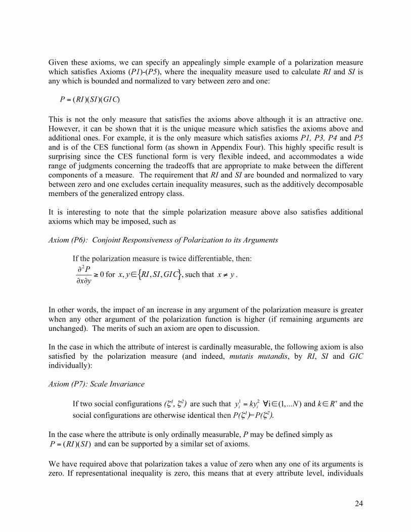
Given these axioms, we can specify an appealingly simple example of a polarization measure which satisfies Axioms (P1)-(P5), where the inequality measure used to calculate RI and SI is any which is bounded and normalized to vary between zero and one: This is not the only measure that satisfies the axioms above although it is an attractive one. However, it can be shown that it is the unique measure which satisfies the axioms above and additional ones. For example, it is the only measure which satisfies axioms P1, P3, P4 and P5 and is of the CES functional form (as shown in Appendix Four). This highly specific result is surprising since the CES functional form is very flexible indeed, and accommodates a wide range of judgments concerning the tradeoffs that are appropriate to make between the different components of a measure. The requirement that RI and SI are bounded and normalized to vary between zero and one excludes certain inequality measures, such as the additively decomposable members of the generalized entropy class. It is interesting to note that the simple polarization measure above also satisfies additional axioms which may be imposed, such as Axiom (P6): Conjoint Responsiveness of Polarization to its Arguments

If the polarization measure is twice differentiable, then:

for such that .

In other words, the impact of an increase in any argument of the polarization measure is greater when any other argument of the polarization function is higher (if remaining arguments are unchanged). The merits of such an axiom are open to discussion. In the case in which the attribute of interest is cardinally measurable, the following axiom is also satisfied by the polarization measure (and indeed, mutatis mutandis, by RI, SI and GIC individually): Axiom (P7): Scale Invariance

If two social configurations (ζ1, ζ2) are such that and the social configurations are otherwise identical then P(ζ1)=P(ζ2).

In the case where the attribute is only ordinally measurable, P may be defined simply as

and can be supported by a similar set of axioms. We have required above that polarization takes a value of zero when any one of its arguments is zero. If representational inequality is zero, this means that at every attribute level, individuals

25

from all groups are represented in exactly the same proportion as they are represented in the population as a whole. As such it is difficult to characterize such a configuration as possessing any polarization. Equally, when group rank sequence position is zero, this means that the distribution of members is perfectly symmetric (i.e. every instance of domination by a member of a group vis-à-vis a member of another group is balanced by a reciprocal instance of domination by a member of the other group vis-à-vis a member of the first group. Once again, while there may be inequality in the society, it would be hard to characterize this situation as one in which there is any polarization between groups. Finally in the accustomed approach to assessing group inequality comparison, if the means of all groups coincide then this contribution is zero, and polarization is equal to zero. When is polarization maximized? RI is maximized when there is complete segregation of groups in the achievement space. Assuming this condition is satisfied, what additional conditions are required to maximize SI? It is easily seen that the maximum value of SI is approached in the limit in which the social configuration is such that one group is as large as possible relative to all others and is disadvantaged relative to all others (specifically in the sense that every member of the disadvantaged group possesses lower achievements than every member of every other group). Assuming this condition too is satisfied, what additional conditions are required to maximize GIC? If the concept of GIC employed is of Type I then the within-group inequalities in the population must be as small as possible. This will be attained when there are no intra-group differences in achievements. Any distribution which satisfies these properties will suffice to approach the maximum level of polarization (for example, that shown in Figure 14a, which depicts three groups with differing population sizes and achievement levels). If the concept of GIC employed is of Type II then the maximum value of GIC is approached in the limit in which the relatively disadvantaged group possesses the lowest possible level of the achievement and the members of other groups possess levels of the achievement which are as high as possible compatible with complete segregation. Thus, if there are two groups one of them must possess the lowest level of the achievement (e.g. zero income) and the other must possess the highest level of the achievement (e.g. all of the income, evenly divided among its members). If there are more than two groups, all groups other than the most disadvantaged must possess distinct achievement levels which are as close as possible to the attainable maximum. Any distribution which satisfies these properties will suffice to approach the maximum possible level of polarization (for example, that shown in Figure 14b, which depicts three groups with differing population sizes and achievement levels in a feasible range). The conclusion as to the circumstance in which polarization is maximized differs from that reached by others. As opposed to Duclos, Esteban and Ray (2004), for example, in which polarization is maximized only when there are two equal sized groups, in our analysis it can be maximized regardless of the number of groups and it is necessary that the most disadvantaged group is as large as possible relative to the others. For polarization to approach its maximum it is required that the poorer group is large relative to the richer groups, there is complete segregation and there is no within-group inequality. Part IV: Conclusion

26

This paper has sought to clarify how one may assess social situations according to the extent to which attributes are disproportionately possessed by different social groups. The measures we have developed capture the various different ways in which experiences of members of distinct groups may differ. Thus, social situations can differ in the extent to which members of a group share experiences with members of other groups (representational inequality), experience the same or different relative positions (sequence inequality) and experience differences in the extent to which interpersonal inequalities are accounted for by inter-group differences (group inequality comparison). These concepts are distinct but complexly interrelated. They each integrate empirical observations and evaluative judgments. Judgments concerning the relative importance to be attached to different aspects of inter-group difference are also involved when they are combined (for example to form a measure of polarization).21 These measures have an intuitive appeal and can have widespread application in social science. There appear to deep-seated tendencies for societies to exhibit segregation, clustering and polarization of identity groups. This observation has important empirical implications and may also give rise to normative concern. For either reason, the concepts and measures we have discussed may prove useful.

21 The concepts we have discussed can be understood as “thick ethical concepts”, on which see Putnam (2004).

27

Acknowledgments We would like to thank a range of persons and institutions for their invaluable assistance in preparing this paper.22

22 We would like to thank for their useful comments or suggestions (without implicating them in errors and imperfections) James Boyce, Rahul Lahoti, Hwok-Aun Lee, Glenn Loury, Yona Rubinstein, Peter Skott, Rajiv Sethi, Joseph Stiglitz, S. Subramanian, Roberto Veneziani and other participants at seminars in the Dept. of Economics at Brown University, the University of Massachusetts at Amherst, the Jerome Levy Institute at Bard College, Queen Mary, University of London and the Brooks World Poverty Institute at the University of Manchester.

28

References Abul Naga, R. H. and T. Yalcin, (2008)," Inequality Measurement for Ordered Response Health Data," Journal of Health Economics 27 (6): 1614-1625. Alesina A and E. La Ferrara (2000), “Participation in Heterogeneous Communities,” Quarterly Journal of Economics, August 2000, 115: 847-904 Alesina A and E. La Ferrara (2002), “Who Trusts Others?” Journal of Public Economics, August 2002, 85: 207-34. Alesina A , A. Devleeschauwer, W. Easterly, S. Kurlat and R. Wacziarg (2003), “Fractionalization,” Journal of Economic Growth, June 2003, 8:155-94 (). Allison, R.A. and J. Foster, (2004) "Measuring Health Inequalities Using Qualitative Data," Journal of Health Economics 23: 505–524.

Anderson, E. (1999), “What is the Point of Equality?” Ethics (1999), pp. 287–337.

Anderson, G. (2004), “Toward an Empirical Analysis of Polarization”. Journal of Econometrics 122 (2004) 1 – 26 Anderson, G. (2005), “Polarization”. Working Paper, University of Toronto. Available at http://www.chass.utoronto.ca/~anderson/Polarization.pdf

Arneson, R. (1989), “Equality and Equal Opportunity for Welfare”, Philosophical Studies (1989), pp. 77-93.

Bartolucci, F., A. Forcina and V. Dardanoni, (2001), "Positive Quadrant Dependence and Marginal Modelling in Two-Way Tables with Ordered Margins," Journal of the American Statistical Association 96(4w56): 1497-1505. Boisso, D., K. Hayes, J. Hirschberg and J. Silber, 1994, "Occupational Segregation in the Multidimensional Case: Decomposition and Tests of Statistical Significance," Journal of Econometrics 61: 161-171.

Cohen, G. A. (1989), “On the Currency of Egalitarian Justice”, Ethics (1989), pp. 906-944.

D’Ambrosio, C. and E. Wolff (2001), “Is Wealth Becoming More Polarized in the United States?” Working Paper 330, Levy Economics Institute, Bard College. Duclos, J-Y., J. Esteban and D. Ray (2004), “Polarization: Concepts, Measurement, Estimation”, Econometrica 1737-1772. Duncan, O.D. and B. Duncan (1955), “A Methodological Analysis of Segregation Indexes”, American Sociological Review, Vol. 20, No.2, pp. 210-217.

29

Dworkin, R. (2000), Sovereign Virtue: The Theory and Practice of Equality, Cambridge, MA: Harvard University Press.

Esteban, J.-M. and D. Ray (1994), “On the Measurement of Polarization”. Econometrica 62, 819–851. Foster, J. and A. Shneyerov (1999), “A General Class of Additively Decomposable Inequality Measures,” Economic Theory, Vol. 14 No. 1. Flückiger , Y. and J. Silber, 1994, "The Gini Index and the Measurement of Multidimensional Inequality," Oxford Bulletin of Economics and Statistics 56: 225-228. Hutchens, R. (1991), “Segregation Curves, Lorenz Curves, and Inequality in the Distribution of People across Occupations”, Mathematical Social Sciences, Vol. 21, pp. 31-51. Hutchens, R. (2004), “One Measure of Segregation”, International Economic Review, Vol. 45, No. 2, pp. 555-578. Jayaraj, D. and S. Subramanian (2006), “Horizontal and Vertical Inequality: Some Interconnections and Indicators”, Social Indicators Research, Volume 75, No. 1, pp. 123-139. Loury, G. C. (2004), The Anatomy of Racial Inequality, Cambridge, MA: Harvard University Press, Miguel, E. and Gugerty, M. (2005) “Ethnic diversity, social sanctions, and public goods in Kenya”, Journal of Public Economics, 89(11-12), 2325-2368. Montalvo, J.G and M Reynal-Querol (2005) “Ethnic polarization, potential conflict and civil war”, American Economic Review, 95 (3), 796-816, June 2005. Østby, Gudrun, (2008) “Polarization, Horizontal Inequalities and Violent Civil Conflict”, Journal of Peace Research, Vol. 45, No. 2, 143-162 Parfit, D. (1997) “Equality and Priority”, Ratio 10, pp. 202-221. Putnam, H. (2004) The Collapse of the Fact/Value Dichotomy and Other Essays, Cambridge MA: Harvard University Press Rawls, J. (1971). A Theory of Justice, Cambridge, MA: Harvard University Press. Rawls, J. (2001). Justice as Fairness: A Restatement, Cambridge, MA: Harvard University Press. Reardon, S.F. and G. Firebaugh, (2002). Measures of Multigroup Segregation, Sociological Methodology, 32, 33-67.

30

Reardon, S. (2008), "Measures of Ordinal Segregation," Working paper 2008-11, Institute for Research on Education Policy and Practice, Stanford University. Forthcoming in Research on Economic Inequality, volume 17. Reddy, S. and A. Jayadev (2011), “Inequalities Between Groups: Theory and Empirics”, forthcoming in World Development, working paper version available on http://papers.ssrn.com/sol3/papers.cfm?abstract_id=1359869 Roemer, J. (1996). Theories of Distributive Justice, Cambridge, MA: Harvard University Press. Schweizer, B. and E. F. Wolff, (1981), "On Nonparametric Measures of Dependence for Random Variables," The Annals of Statistics, 9(4): 879-885. Sen, A. (1992), Inequality Reexamined, Cambridge, MA: Harvard University Press. Shorrocks, A.F (1980), “The Class of Additively Decomposable Inequality Measures”, Econometrica, Vol 48 (3), 613-25. Shorrocks, A.F (1983), “Ranking Income Distributions”, Economica, 50, 3-17. Silber, J G.,(1989). "On the Measurement of Employment Segregation," Economics Letters, Elsevier, vol. 30(3), pages 237-243, September. Silber, J G. (1991). “Inequality Indices as Measures of Dissimilarity: A Generalization," Statistical Papers, 1991, 32:223-231. Silber, J.,G (1992), "Occupational Segregation Indices in the Multidimensional Case: A Note," Economic Record 68: 276-277. Stewart, F.(2001). “Horizontal Inequalities: A Neglected Dimension of Development” WIDER Annual Lectures 5, UNU WIDER Wang, Y.Q. and Tsui, K.Y. (2000), “Polarization Orderings and New Classes of Polarization Indices,” Journal of Public Economic Theory ,349—363 Subramaniam S (2009). Alternative Approaches To Reckoning Group Disparities In Distributional Analysis: Concepts, Measurement, And Illustrative Applications”, Madras Institute of Development Studies, Mimeo. Tchen, A. H., (1980), "Inequalities for Distributions with Given Marginals," The Annals of Probability 8(4): 814-827. Wolfson, M.C. (1994), “When Inequalities Diverge”, American Economic Review Papers and Proceedings 94.353-358. Zhang, X. and R. Kanbur (2001), “What Difference Do Polarisation Measures Make? An Application to China,” Journal of Development Studies, 37. 85—98.

31

32

Figures

33

34

35

36

37

38

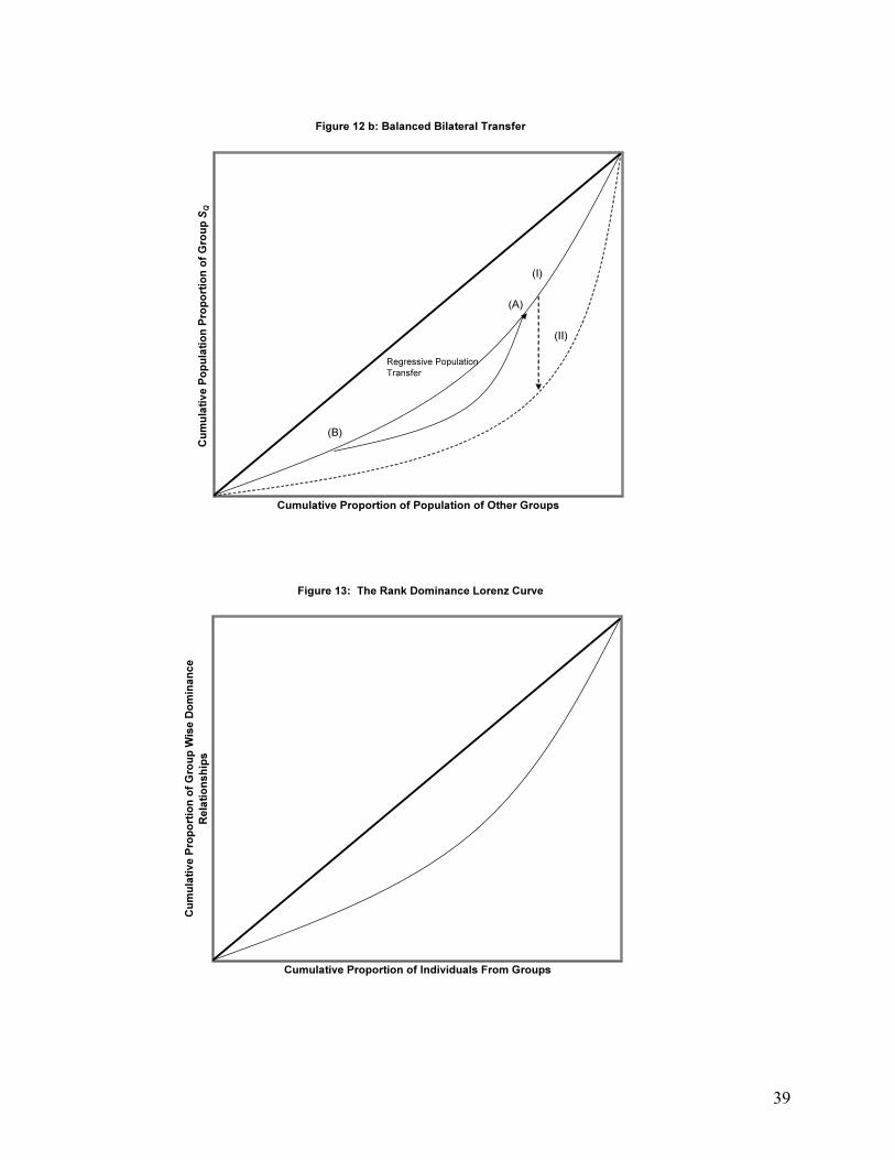
39

40

APPENDICES Appendix One: Moral Reasoning and Inter-Group Differences

41

Should inter-group differences be disvalued? We have argued above that there are both intrinsic and instrumental reasons that might be appealed to in answering this question. The instrumental reasons need not depend on any direct concern with the relative well-being of groups since they can be purely derivative of a concern for individual advantage (insofar as such advantages are causally affected, through various mechanisms, by their distribution across the different groups in society to which individuals belong). The moral justification for such concern is consequently dependent only on there being moral reason to favor a particular distribution of individual advantages with regard to which inter-group differences play a causal role. In contrast, the perspective in which inter-group differences are intrinsically disvalued is more challenging to justify. This perspective appears to contrast with that advocated in standard "individualist" approaches to social assessment, which are embodied in social choice theory and in moral philosophy. For example, the "anonymity axiom" in social choice theory is typically interpreted to demand that permutations of individual advantages across persons, whatever groups they may each belong to, should not have any effect on assessments of the desirability of social states of affairs. Such an approach appears to rule out any direct concern for inter-group differences (on which, see for example Loury, 2004). A thought experiment may be helpful in investigating the appropriate role that group related considerations should play in social assessment. We may imagine an "original position" of the general type described by Rawls (1971) or other theorists in the modern contractarian tradition of moral philosophy. Imagine that the parties to this original position (perhaps trustees choosing alternative social arrangements on behalf of specific individuals who will ultimately inhabit them, along the lines defined by Rawls (2001)) engage in bargaining with each other about future social arrangements in one of two different situations. In the first situation, the trustees know only that the individual who they represent will eventually occupy a particular position in a well-defined distribution of individual advantages, where that distribution depends on the particular choice of social arrangements made by the trustees and where a particular position in society is assigned to each individual through a "lottery". In the second situation, the trustees know that the individual that they represent will be assigned to a particular rank in a specific social group in a "first round lottery", and that each social group will be assigned to occupy a particular set of positions in a social distribution of advantages in a "second round lottery"23. Suppose that the expected final distribution of individual advantages (disregarding group membership) is expected to be identical in the two situations, given a specific choice of social arrangements by the trustees. Suppose further that the second situation is such that as a result of the second round lottery systematic differences in the possession of individual advantages between members of distinct groups are expected to result. No such systematic differences would normally be expected to result from the lottery implemented in the first situation. By construction, the outcomes resulting from the social arrangements put in place in the first situation will be ones in which there are no systematic inter-group differences of the kind that are present in the outcomes resulting from the second situation, although the distribution of

23 We abstract from the issue of relative sizes of groups here.

42

individual advantages is identical. Should any moral distinction be made between these two cases? It seems clear that the parties to the original position would have no reason to prefer one situation over the other if they are concerned only about the individual advantages that are distributed, since the individuals who they represent have an identical chance in either case of occupying any given position. If there is reason to prefer the first situation over the second it must have to do either with the concern that systematic inter-group differences are likely over time to have causal effects which merit moral attention which have not otherwise been considered (for example by leading to internalized stigma or other psychological effects on individuals, or the entrenchment over generations of social inequalities between groups) or with a view that group membership is a morally salient feature to be taken account of in the assessment of the distribution of individual advantages quite apart from its effect on individual lives. An attempt to justify the latter perspective might employ a conception in which such non-individualistic considerations play a role (on which see e.g. Parfit, 1997, on “telic” and “deontic” approaches to the assessment of inequality). Of course, the device of the original position may only have partial relevance to the moral assessment of actual empirical cases. In practice, distributions of individual advantage derive from historical processes, some of which may have involved systematic and perhaps grievous harm done by members of a given group toward members of another group. In such a case, considerations of historical reparation and other moral concerns related to the rectification of historical injustice may play a role in the justification of moral concern for inter-group differences.

43

Appendix Two (Rank Domination Quotient and Average Rank) As we noted above, the average rank of a group (call it , ) is also an indicator of group rank sequence position. In fact, it is linked in a direct and monotonic fashion to group rank dominance. As before, we understand rank as referring to the position in which an individual appears when incomes are sequenced from lowest to highest (the ascending order of values). When individuals from the same group share an income we shall assign them a rank equal to the average position in which an individual appears when incomes are sequenced from lowest to highest. We shall consider subsequently the rule to be applied in assigning ranks when individuals from different groups share an income. Consider at the outset, for simplicity, a perfectly segregated population in which there is no more than one individual in each income bracket. In such a population, the total number of instances of pair-wise rank domination that members of group J enjoy vis-à-vis others can be understood as a function of the ranks of members of group J in the population. The lowest ranked member of group J, having rank r1 dominates (r1-1) persons belonging to other groups. The second lowest ranked member of group J, having rank r2 dominates (r2-2) persons belonging to other groups (i.e. (r2-1) persons belonging to all groups -1 person belonging to the same group)). Extending this logic, the total number of instances of pair-wise domination by members of group J is:

The rank domination quotient correspondingly is

from which it follows that:

.

It is easy to see that this formula also applies in the case in which there may be more than one person in an income bracket but all persons who share an income bracket are always from the same group. In contrast, in the most general case of populations in which there may exist some income brackets which contain members of distinct groups there can be ties in the income ranks assigned to members of different groups, which will imply that this formula will no longer hold exactly unless the ranks are assigned appropriately to individuals in the same income bracket. Specifically, if strict domination is the concept that is employed then this relationship will hold exactly if individuals in the same income bracket are assigned a rank equal to the lowest of their positions in the ascending order of values. Correspondingly, if weak domination is the concept that is employed then this relationship will hold exactly if each individual in the income bracket is assigned a value equal to the sum of the lowest of the positions of the individuals sharing the

44

income bracket (in the ascending order of values) and the number of individuals from other groups with whom they share the income bracket. The correspondence we have derived between and holds also in the case of continuous distributions, as can be shown through limit properties. In this case, the average rank of members of a group, J, is defined by

and the rank domination quotient for the group is defined by: Where is the cumulative distribution function for incomes of the entire population, is the density function for incomes of members of the group, J, and the integrals are calculated over the domain of all possible incomes.

45

Appendix Three (Proof of Lemma 1) Without loss of generality, we shall assume that the attributes can be understood as income levels. Let A refer to a matrix of size K by n with K identity groups and n income levels. Each element in the matrix . We say that the ith identity group is ‘under-represented’ at the jth income level if the proportion of persons from group i at income j is less than the proportion of persons of group i in the population as a whole. We denote the statement that the ith identity group is ‘under-represented’ at the jth income level by . We say further that that the ith identity group is ‘over-represented’ if the proportion of persons from group i at income j is greater than the proportion of persons of group i in the population as a whole. We denote the statement that the ith identity group is ‘over-represented’ at the jth income level by

. If the ith identity group is represented at the jth income level in the same proportion as it is represented in the population as a whole then we say that it is “equiproportionally represented” and we denote this by . Thus A is a matrix in which every element is 0,1 or 2. We may further note that if any row or any column contains a zero then it must contain a one and vice versa. This requirement captures the necessity that if an identity group is overrepresented at an income level, it must be underrepresented at another income level and that if a group is overrepresented at an income level then another group is under-represented at that same income level. A balanced bilateral transfer is always possible if an identity group is represented to a greater extent at one income level (call it y1) than it is at another (call it y2) and another identity group is represented to a lesser extent at y1 than it is at y2. This condition is satisfied as long as it is possible to identify two rows (i and j) and two columns (l and m) of the matrix A such that they

form a matrix A~= which is of one of the following forms, or which can be constructed

from one of the following forms by permuting either their rows or their columns:

, , , , .

The lemma is therefore equivalent to the statement that there exists a matrix A~ for any matrix A which contains at least a single one or zero. Suppose that the lemma is false. Then, it is possible to construct an A such that there is no A~ associated with it. We now try to construct such a matrix A. Without loss of generality consider the case in which A contains at least one zero (i.e. an identity group is under-represented at a particular level of income). We can present this as occurring at the top left corner (a11)of the matrix, without loss of generality, as below:

46

A=

This however means that there must be at least one level of income in the first column and in the first row in which there is over-representation of an identity group. Without loss of generality, let us say that this occurs at a12 and a21 respectively so that

A=

Now if a22 = 0 or 2 then A~ exists. If a22 0 or 2 then a22 = 1. That is

A=

Consider row 2 and column 2 now. Since for the already fixed elements, there is over-representation, there must be elements in row 2 and in column 2 respectively that have value zero (reflecting under-representation). Without loss of generality, let these occur at a23 and a32 respectively so that

A= =

But this in turn fixes a13, a31 and a33 to be 0 since if any of these are 1 or 2, we can construct matrix A~ . This in turn implies that there exist elements elsewhere in row 3 and column 3 with value 1 (indicating over-representation), which we can place without loss of generality at a34 and a43, respectively. It can readily be seen that this in turn fixes a41, a42 , a44, a24 and a14 to be 1 since if any of these are 0 or 2, we can construct matrix A~ . Thus we may construct a matrix A such that aij= aji =0 if i is odd and and aij=1 otherwise. Let us now consider the matrix where the row (k-1) is odd. This means that A has the form

47

A=

This in turn implies that ak-1,n =1 and ak,n-1 =1. It may be verified that for A~ not to exist all elements in row k and in column n must equal 1. However, this violates the requirements on a matrix A. Consider now the matrix where the row (k-1) is even. This means that A has the form

A=

This in turn implies that ak-1,n =0 and ak,n-1 =0. It may be verified that for A~ not to exist all elements in row k and in column n must equal 0. However, this violates the requirements on a matrix A. Thus it is not possible to construct a matrix A such that A~ does not exist. A~ must exist, thereby proving the lemma. QED

48

Appendix Four: The Multiplicative Polarization Function in the CES Family Proposition: The only Polarization function which satisfies Axioms P1, P3, P4, and P5 and belongs to the CES family of functions is the multiplicative form , where RI and SI are calculated using an inequality measure which has a range between zero and one Proof: By Axiom P1 it is a function of all three arguments and only those. Since the Polarization measure is a member of the CES family it can be taken to have one of the forms:

i. with β > 0. ii. iii. It is easy to check that functions of form (i) fail Axiom P3, and functions of form (iii) fail Axiom P5. What about functions of form (ii)? By Axiom P4 , the coefficient A must have value 1 and by Axiom P3, the exponents must also have value 1. Thus, form (ii) collapses to the pure multiplicative form . It may be checked that this function satisfies all of the axioms. QED It may be noted that if Axiom P3 is dropped then the function is admissible. This may be attractive from the viewpoint that the values of the polarization index which are produced are in of the same order of magnitude as the component parts of the index. If Axiom P3 is dropped then functions of form (i) cannot be excluded. However, if it is required that Axiom P2 be satisfied then functions of form (i) can be excluded. It follows that functions of the form are the only members of the CES family which satisfy Axioms P1, P2, P4, and P5, where RI and SI are calculated using an inequality measure which has a range between zero and one. If Axiom P3 is dropped and additionally Axiom P4 is adjusted so that there is no requirement that the index of polarization take on a maximum value then a broader range of inequality measures can be used to calculate RI and SI, such as the additively decomposable generalized entropy measures (which are unbounded above).