Industrial Evolution in Crisis-Prone Economies

Eric BondVanderbilt University

James TyboutPennsylvania State University and NBER

Hâle UtarPennsylvania State University

Crises-Prone Economies

• Since the early 1980s, currency crashes and banking crises have tended to occur together (Kaminsky and Reinhart, 1999).

• Possible reasons:– External shocks coupled with a fixed exchange rate can trigger

loss of reserves, credit crunch, and bankruptcies.

– Financial sector problems can trigger a bail-out, excessive money creation, and a currency crash.

– Exchange rate-based stabilization plans induce rapid capital inflows, squeeze tradeables producers and eventually inspire speculative attacks.

Firm-level consequences

• Crisis-prone macro environments create:– Big swings in intensity of import competition and export

earnings.

– Big swings in costs of finances.

• Consequences– Ability to survive and grow depends upon collateral.

– With risk-averse households, size of initial wealth also affects desire to own firms.

– Industrial growth and productivity-based selection processes are affected.

• Our Objective: Quantify these forces

The exercise

• Fit VAR switching model to time series on exchange rates (e) and interest rates (r).

• Fit establishment-level profit functions to panel data on textiles producers.– Links profits to capital stocks, productivity, exchange rates and

interest rates– Characterizes producer-specific productivity shocks

• Calibrate by searching over entry costs, fixed costs, and degree of credit market imperfections.

• Simulate industrial evolution patterns under alternative macro scenarios.

The Model: Overview

• Basic features of our model:– Partial equilibrium; macro variables exogenous.

– No secondary equity markets.

– Risk-averse, forward-looking households allocate their wealth between proprietorships and bank deposits.

– Households are heterogeneous in terms of their management opportunities and wealth.

– Those that do operate businesses can borrow to expand their businesses, subject to collateral constraints.

The Model: Primitives

• Given current wealth (ait), each household chooses whether to operate a proprietorship.

• At the beginning of period t, household i decides how to allocate its wealth (ait) between

– investments in its firm (kit) and

– bank deposits (ait- kit), which earn at rate rt.

• Negative bank deposits amount to bank loans, which are

used to finance business investments.

The Model: Primitives

• Operating profits before interest:

• Exogenous transition densities

00

0)()exp(),,( 10

it

itititittittit kif

kifkfkReek

)|( 1 itit

),|,( 11 tttt rere

The Model: Primitives

• Utility:

• Consumption:

1)(

1it

itc

cU

)()(),,( 10 itititittittitiit aakarekyc

The Model: Optimization

• Households choose current savings and capital stock to maximize:

subject to a borrowing constraint, and recognizing that threshold costs are associated with the creation of a new firm.

t

tiiiiiiit aakarekyUE

)()(),,( 10

The Model: Optimization

• The borrowing constraint (Banerjee and Newman, 1993):

– Firms’ productivity levels are public knowledge, so lenders know how much they can earn if the household invests its loan in the firm.

– But households can sell their firms and abscond with ∙kit , 0<<1.

– Banks do not make loans sufficiently large that this is the borrower’s best option.

The Model: Optimization

• If household i owns a firm, and it shuts this firm down in period t, its expected present value of utility is:

),,,(),|,()(max

),,,(

000

0

reyaVrereaaaryU

reyaV

ir

Ett

eitittia

ttiitE

The Model: Optimization

• The unconditional expected utility for firm owners is thus

• Where VI (∙) is the value of continuing to operate:

,),,,,(),,,,,(max),,,,( 000 ttiitE

itttiitI

itttiit reyaVvreyaVvreyaV

.)|(),|,(),,,,(

)()(),,(max

),,,,(

0

00,0

0

rittti

e

ititittittitika

itttiitI

vrerereyaV

aakarvekyU

vreyaV

it

The Model: Optimization

• The max problem for the continuation value is subject to

the no-default constraint:

),,,,(

)|(),|,(),,,,(

)()(),,(

0

0

0

itttiitE

rittti

e

ititittittiti

reykV

vrerereyaV

aakarvekyU

The Model: Optimization• Households that do not own firms create them if:

>

where F is the sunk cost of establishing a new firm.

)()|(),|,(),,,,(

)()(),,(max),,,(

00

00,00

qrerereyaV

aarkaekFyUreyaN

V

rtti

e

ittitittitikai it

.),|,(),,,(),,,,(max

)(max),,,(

00

000

e rtti

Oi

N

ittitiaiO

rerereyaVreyaV

aarayUreyaV

Estimating the Profit Function

• Production technology:

Revenue function:

Variable cost function:

itititit lkuQ )exp(

11

)1()1(

1* )1(exp

itit

itititit k

w

PwuC

11

)1()1(

11* )1(exp

itit

itititit k

w

PwuG

Estimating the Profit Function

• Let be a Cobb-Douglas function of a time trend, the real exchange rate, and firm-specific shocks.

• Assume that revenues and variable costs are measured with noise, each of which can be serially correlated.

)1/(1/ ititit wPw

Git

Eititt

Git KteG ln)ln( 3210

Cit

Eititt

Cit KteC ln)ln( 3210

Variable Coefficient Std. Error Z-ratioLevel-form estimator

Exchange rate -0.329 0.038 -8.722

Capital stock 0.201 0.007 29.400

Trend term 0.007 0.003 2.038

Initial year dummy -0.015 0.013 -1.196

Intercept, revenue equation 8.570 0.207 41.428

Intercept, cost equation 8.319 0.207 40.221

Variance of innovations in εE process 0.130 0.004 31.287Root of εE process 0.937 0.007 143.980Variance of innovations in εC process 0.027 0.003 8.072Root of εC process 0.260 0.022 11.987Variance of innovations in εR process 0.026 0.004 6.002Root of εR process 0.728 0.022 32.858

Number of observations 2,640

Profit Function Parameters

Estimating the VAR

• Define

• The VAR:

where and switches between regimes are governed by the transition matrix p = {pmn}.

• Restricted version: only the covariance matrix varies between regimes.

t

tt r

ey

mtt

mmt yy 110

mmt

mtE

Parameters e r

Intercepts (0)0.012(0.03)

0.031(0.01)

AR coefficients (1)0.996

(0.006)0.028(0.02)

-0.006(0.002)

0.953(0.011)

, Non-crisis periods3.94 e-4 -1.34 e-5

-1.33 e-5 7.01 e-5

, Crisis periods

9.25 e-3 -2.82 e-4

-2.82 e-4 2.69 e-3

P0.965 0.035

0.598 0.410

Log likelihood 1472.83

H0: same as simple VAR model = 363.59

H0: MSH and MIASH are same =18.80

Switching VAR, Macro Processes

)12(2

)4(2

Simulations (preliminary)

• Compare two macro environments

– Estimated:

– More crisis-prone:

• Simulate behavior over 300 periods, repeat 100 times and average

410.0598.0

035.0965.0P

5.05.0

5.05.0P

Simulated macro series

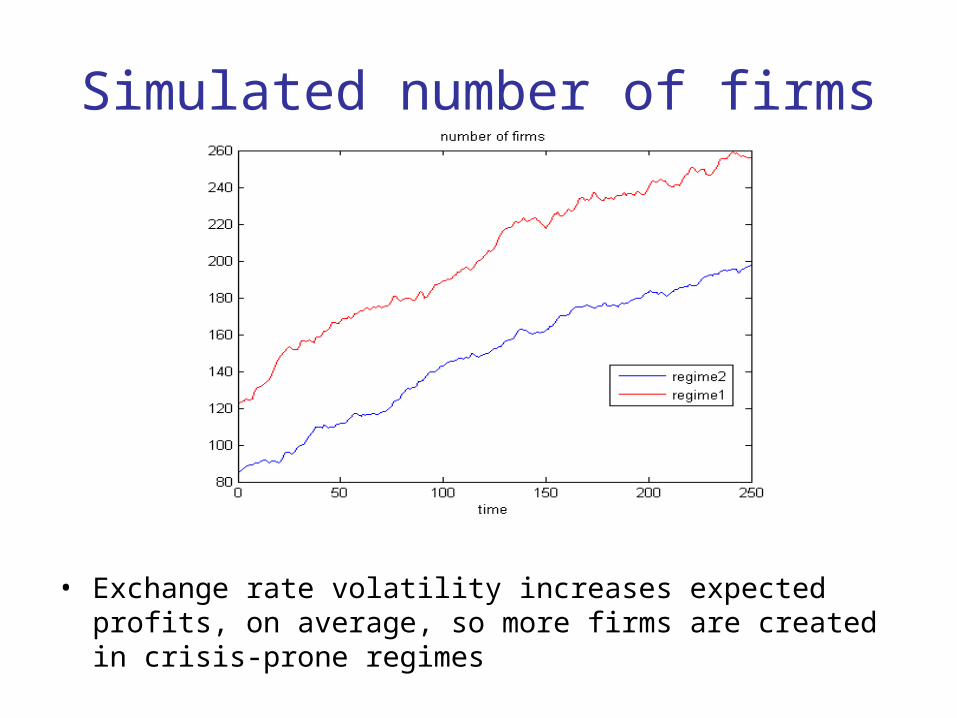
Simulated number of firms

• Exchange rate volatility increases expected profits, on average, so more firms are created in crisis-prone regimes

Simulated entrants

Simulated exits

Simulated net entry

Simulated productivity

• In crisis-prone economies, selection puts heavier weight on wealth of owners and less weight on productivity.

Wealth of entrepreneurs who exit

• In crisis-prone regimes, exiting firms are more commonly held by households with modest wealth

Simulated capital and wealth of owners

• Average firm size is larger in crisis-prone environments, but average household wealth is smaller.

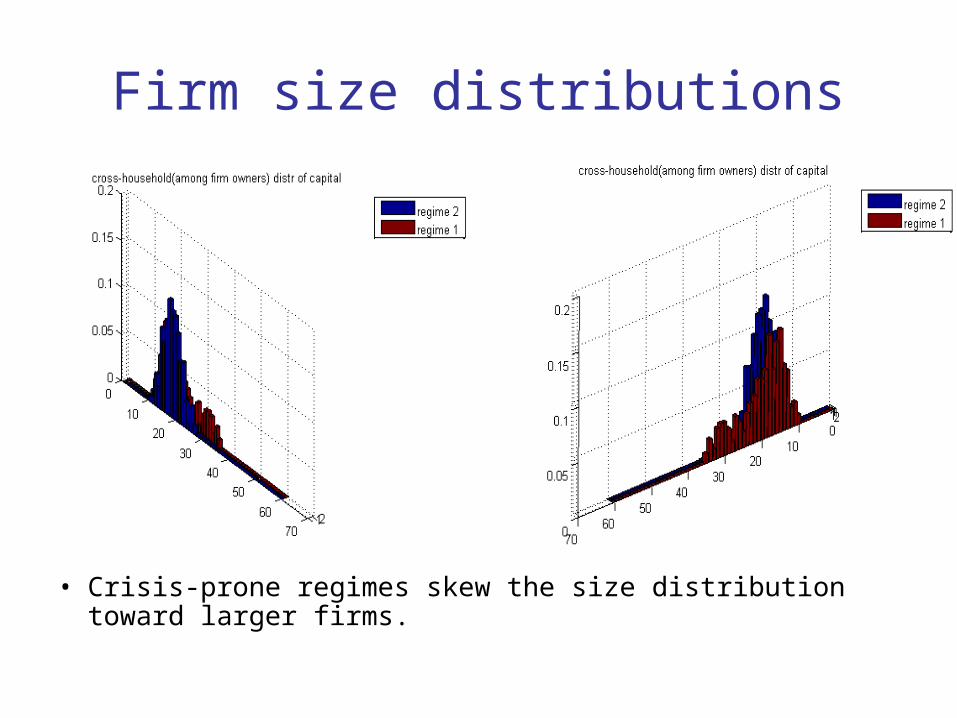
Firm size distributions

• Crisis-prone regimes skew the size distribution toward larger firms.

Leverage distributions

• Crisis-prone environments induce higher leverage among large firms.

Concluding remarks

• Results are very preliminary

– Not all of the model’s parameters have been estimated yet

– The counter-factual crisis-prone environment may not be realistic

• Nonetheless, it does establish that the mix of industrial sector firms is potentially sensitive to the macro environment, and

• The effects of crisis-prone environments depend upon:

– Wealth distributions

– Risk aversity

– Credit market imperfections