inducing safer oblique trees without costsusir.salford.ac.uk/944/2/expertsystems_2005.pdf · ·...
TRANSCRIPT

Inducing safer oblique trees without costsVadera, S
http://dx.doi.org/10.1111/j.14680394.2005.00311.x
Title Inducing safer oblique trees without costs
Authors Vadera, S
Type Article
URL This version is available at: http://usir.salford.ac.uk/944/
Published Date 2005
USIR is a digital collection of the research output of the University of Salford. Where copyright permits, full text material held in the repository is made freely available online and can be read, downloaded and copied for noncommercial private study or research purposes. Please check the manuscript for any further copyright restrictions.
For more information, including our policy and submission procedure, pleasecontact the Repository Team at: [email protected].
Inducing Safer Oblique Trees without Costs
Sunil Vadera [email protected] of Computing, Science and Engineering,University of Salford, Salford M5 4WT, UK
Abstract
Decision tree induction has been has been widely studied and applied. In safety appli-cations, such as determining whether a chemical process is safe, or whether a person has amedical condition, the cost of misclassification in one of the classes is significantly higherthan the other class. Several authors have tackled this problem by developing cost-sensitivedecision tree learning algorithms or suggested ways of changing the distribution of trainingexamples to bias the decision tree learning process so as to take account of costs.
A pre-requisite for applying such algorithms is the availability of costs of misclassifica-tion. Although this may be possible for some applications, in the area of safety, obtainingreasonable estimates of costs of misclassification is not easy.
This paper presents a new algorithm for applications where the cost of misclassificationscan not be quantified, though the cost of misclassification in one class is known to besignificantly higher than another class. The algorithm utilises linear discriminant analysisto identify oblique relationships between continuous attributes and then carries out anappropriate modification to ensure that the resulting tree errs on the side of safety.
The algorithm is evaluated with respect to ICET, one of the best known cost-sensitivealgorithms, OC1 a well known oblique decision tree algorithm and an algorithm that utilisesrobust linear programming.
1 Introduction
Research on decision tree learning is one of the major successes of AI, with many commercialproducts, such as case based reasoning systems (Kolodner, 1993) and data mining toolsutilising decision tree learning algorithms (Berry & Linoff, 2004). Early research in thisarea developed algorithms that aimed to maximize overall accuracy. More recent researchis being influenced by recognising that human decision making is not focused solely onaccuracy, but also takes account of the potential implications of a decision. For example, achemical engineer considers the risks of explosion when considering the safety of a processplant, a bank manager carefully considers the implications of a customer defaulting on aloan and a medical consultant does not ignore the potential consequences of misdiagnosing apatient. This motivation has led to research in the area of decision tree learning progressingfrom considering accuracy alone, to the development of algorithms that minimize costs ofmisclassification (e.g., Breiman, Friedman, Olsen, & Stone, 1984; Turney, 1995).
Research on this problem can be categorised into two broad approaches: algorithms thataim to reduce a cost-sensitive problem to an equivalent accuracy maximization problem,and those that extend accuracy based algorithms to handle costs of misclassification. 1
1There are, of course some approaches that don’t use decision trees at all, but these are outside the scopeof this paper.
1

The first category of systems includes the proposal by Breiman et al. (1984), who sug-gested changing the distribution of the training examples to be equivalent to the ratio ofcosts of misclassification. More recently, Zadrozny, Langford, and Abe (2003) formalizethis idea, called stratification, and show how the distribution of examples can be changedto implicitly reflect the costs and thereby enable the application of accuracy based classi-fiers. However, Elkan (2001) shows that an impurity measure, with a similar basis to thoseadopted in many of the decision tree learning algorithms (such as CART (Breiman et al.,1984) and C4.5 (Quinlan, 1993)) is insensitive to stratification, therefore casting doubt onthe effectiveness of using such systems after changing the distribution of examples.
The second category of systems is based on the observation that decision tree learningalgorithms that aim to maximize accuracy construct trees in a greedy, top-down manner andutilize an information-theoretic measure to select decision nodes. Hence, a natural approachto cost-sensitive decision tree construction is to alter the information-theoretic selectionmeasure so that it includes costs. A number of systems take this approach, includingthe EG2 (Nunez, 1991), CS-ID3 (Tan, 1993) and ICET (Turney, 1995). The studies byPazzani, Merz, Murphy, Ali, Hurne, and Brunk (1994) and Turney (1995) include empiricalevaluations of these types of algorithms. Pazzani et al. (1994) conclude that these algorithmsare no more effective than algorithms that ignore costs. Turney (1995) develops ICET, analgorithm based on using Genetic Algorithms (GAs) to evolve cost-sensitive trees that aimto take account of both costs of misclassification as well as costs of tests. Turney evaluatesICET with respect to several algorithms and shows that ICET performs better than theother algorithms, though he also notes the difficulty ICET has for domains where costs ofmisclassification are not symmetric:
“it is easier to avoid false positive diagnosis (a patient is diagnosed as being sick,but is actually healthy) than it is to avoid false negative diagnosis (a patientis diagnosed as healthy, but is actually sick). This is unfortunate, since falsenegative diagnosis usually carry a heavier penalty, in real life.” 2
Thus, the problem of developing an effective cost-sensitive decision tree algorithm whengiven costs of misclassification remains a difficult and open problem. Even if there is aneffective algorithm for minimising costs of misclassifications and costs are available, thereis a further potential problem which we now illustrate. Consider the application of a de-cision tree induction algorithm on the Diabetes data set, which has been widely used forbenchmarking. The data set has 768 examples of which 65% are in the safe class (i.e., nodiabetes) and 35% are in the unsafe class (i.e., has diabetes). Suppose we use 50% of thisdata for training and 50% for testing, then decision tree algorithms would typically producethe results given in table 1.3
If, say, the cost of misclassifying unsafe cases was four times that of misclassifying safecases, then the expected cost and accuracy are:
Expected Cost =50 ∗ 1 + 59 ∗ 4
384= 0.75
2Turney refers to a simple cost matrix as one where the costs of misclassifications are equal, and a complexcost matrix as one where the costs are different.
3These particular results were obtained with 10 random trials using an axis-parallel algorithm similar toC4.5 and the literature contains similar results.
2

Class Algorithm Algorithmreturns Safe returns Unsafe
Actually Safe 200 50Actually Unsafe 59 75
Table 1: Typical results produced for the diabetes data set
Accuracy =275384
= 71.6%
However, a trivial algorithm that always returns the unsafe class would result in:
Expected Cost =250 ∗ 1 + 0 ∗ 4
384= 0.65
Accuracy =125384
= 32.6%
Thus, as this example illustrates, if a learning algorithm aims to minimise the cost, there isa danger that it will achieve this by sacrificing overall accuracy significantly. Of course, ifthere was an algorithm that produced high accuracies for both classes, then there is no needto sacrifice accuracy in one of the classes and indeed, no need for cost-sensitive algorithms,since accuracy based algorithms would suffice.
Given this motivation, this paper presents an alternative algorithm that aims to improvethe accuracy of the unsafe class whilst aiming to retain overall accuracy and which does notrequire the costs of misclassifications.
The paper is organised in two main parts: section 2 develops the algorithm and section 3presents an evaluation of the algorithm with respect to three other decision tree algorithmson six data sets.
2 Development of a Safer Induction Algorithm
The central idea of the algorithm is to err on the side of caution and aim to avoid concludingthat a process or situation is safe without supporting examples. This aim is not easy toimplement with current algorithms as we now illustrate. When faced with continuousattributes, most decision tree learning algorithms discretise the attributes resulting in whatare known as axis-parallel splits (such as in C4.5 (Quinlan, 1993) and Remind (Althoff,Auriol, Barletta, & Manago, 1995)). 4
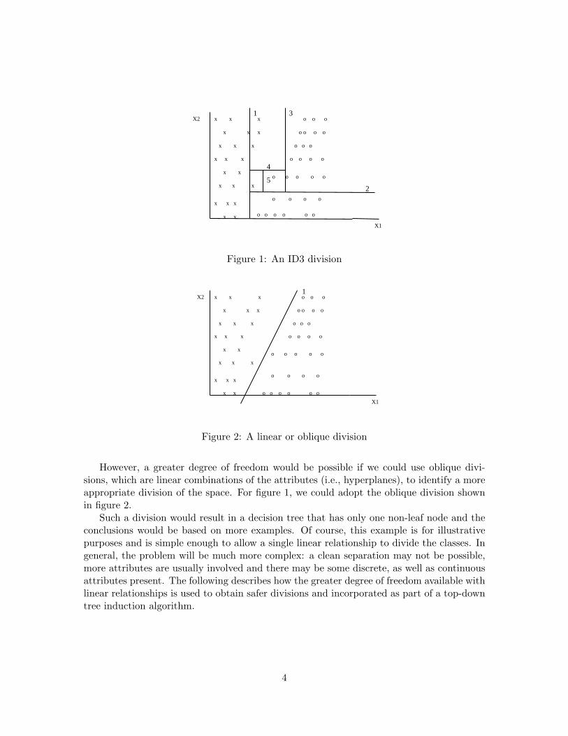
Figure 1 illustrates what happens when axis-parallel splits are used in an example wherethere are two classes denoted by ‘x’ and ‘o’. Line 1 represents the first division, line 2 thesecond division, and so on. Consequently, the decision tree for this example would have 5non-leaf nodes (one for each dividing line) and 6 leaf nodes for the conclusions (one for eachregion). Thus, to achieve our aim of not drawing conclusions about a region being safe, theonly freedom we have is to move the lines along each of the axes.
4The exceptions, CART and OC1 are considered later.
3
x x x
x x x
x x x
x x x
x x
x x x
x x x
o o o
o o o o
o o o
o o o o
o o o o
o o o o
o o o o o ox x
X2
X1
1
2
3
o
4
5
Figure 1: An ID3 division
x x x
x x x
x x x
x x x
x x
x x x
x x x
o o o
o o o o
o o o
o o o o
o o o o
o o o o
o o o o o ox x
X2
X1
1
o
Figure 2: A linear or oblique division
However, a greater degree of freedom would be possible if we could use oblique divi-sions, which are linear combinations of the attributes (i.e., hyperplanes), to identify a moreappropriate division of the space. For figure 1, we could adopt the oblique division shownin figure 2.
Such a division would result in a decision tree that has only one non-leaf node and theconclusions would be based on more examples. Of course, this example is for illustrativepurposes and is simple enough to allow a single linear relationship to divide the classes. Ingeneral, the problem will be much more complex: a clean separation may not be possible,more attributes are usually involved and there may be some discrete, as well as continuousattributes present. The following describes how the greater degree of freedom available withlinear relationships is used to obtain safer divisions and incorporated as part of a top-downtree induction algorithm.
4

Following the intuition suggested by the above example, the aim is to identify a linearcombination of the form:
m∑
j=1
aj xj ≤ c (1)
where m is the number of continuous attributes, aj are the coefficients, xj are the valuesof the continuous attributes and c is the threshold. This linear combination should be suchthat it “best” separates the two classes. By “best” we mean the division that minimizesthe probability of incorrectly classifying an example.
With this interpretation of “best”, we can use a well known statistical technique, calledthe linear discriminant method, for identifying the initial form of such relationships. Asdescribed below, the identified relationship is then modified so that the resulting decisiontree errs on the safe side.
The linear discriminant method enables us to find relationships like (1) by using thefollowing equation (Morrison, 1976):
xtΣ−1(µ1 − µ2)− 12(µ1 + µ2) ≤ ln
(P (C2)P (C1)
)(2)
where x is a vector representing the new example to be classified, µ1, µ2 are the meanvectors for the two classes, Σ is the pooled co-variance matrix, and P (Ci) is the probabilityof an example being in class Ci.
Theoretically, it can be shown that this equation minimizes the misclassification ratewhen x has a multivariate normal distribution and when the co-variance matrices for each ofthe two groups are equal (this is sometimes known as the homogeneity condition). Althoughin practice, this equation is sometimes used without testing these optimality conditions,there remains a danger that it could give poor results if the data departs far from theseconditions. Hence later, when we incorporate such linear discriminants into a decision treelearning algorithm, we will guard against this possibility.
In the context of safety, we need to ensure that the linear discriminant obtained bythe above equation is on the safe side. In particular, there may be situations where theclasses overlap and it is not possible to separate them using a hyperplane. Since the lineardiscrimination method minimizes the probability of an error, it may misclassify some of theexamples of both classes. Figure 3 illustrates this problem for a two-attribute and two-classproblem.
If we adopt such a linear split, each of the regions would be further sub-divided by theID3 based algorithms and therefore result in a smaller version of the kind of problem weillustrated in figure 1. To reduce this, we can adjust the linear discriminant so that onlyone of the regions requires further sub-divisions. In making such an adjustment, we have achoice:
1. Adjust the discriminant so that one of the regions has just unsafe examples.
2. Adjust the discriminant so that one of the regions has just safe examples.
If we choose the second alternative, there may be a few safe examples in a region thathas numerous unsafe examples. Hence, at some point, the learning algorithm will further
5

x x x
x x x
x x x
x x x
x x
x x
x x x
o o o
o o o o
o o o
o o o o
x x
X2
x
X1
A
ox
o Unsafex Safe
o x
xx
o
o
x
x
Figure 3: An illustration of overlapping classes
sub-divide the unsafe region and isolate part of that region as safe. That is, a region wouldbe inferred as safe based on just a small number of examples which is contrary to ouraims. As an illustration of this effect, figure 4(a) shows the regions identified when weapply this approach on figure 3. Notice that the region on the right of line A and belowline B is considered as safe based on just two examples. In contrast, if we select the first
o
X2
x
xx
o
o
X1
A
Bx
x
Safe Region
UnsafeSafeRegion Region
(a) An unsafe linear adjustment.
o
X2
x
xx
o
o
X1
B A
x
xC
Safe
Unsafe
UnsafeSafeRegion
Region
Region
Region
(b) A safer linear adjustment.
Figure 4: An illustration of adjustments
alternative, some regions may be inferred as unsafe based on a small number of examples.As an illustration, figure 4(b) shows the effect of applying this approach on figure 3.
Hence, since we wish to err on the side of safety, we prefer to adjust the discriminanttowards the first alternative. To achieve this, the linear discriminant is adjusted by changinga coefficient (i.e., one of ai, or c in equation (1)) in a way that captures the furthestmisclassified safe example and results in the best separation (as measured by the informationgain). That is, equation (1) is used to compute a new value for each coefficient so that
6

it excludes the furthest misclassified safe example and by keeping the other coefficientsconstant. The new coefficient that results in the best division is then adopted.
Once we have this method for identifying suitable linear divisions and adapting them toerr on the safe side, we need to incorporate it within the usual inductive learning algorithmused by the ID3 family. This is done in a manner that remains faithful to the principle be-hind ID3 based algorithms. That is, from the available divisions: axis-parallel splits, lineardivision and the other attributes, we select the one that maximizes the information gained.Adopting this view gives added protection against situations where the data does not satisfythe theoretical conditions that guarantee a minimum probability of misclassification (i.e.,the homogeneity condition described above), since the algorithm can default to the usualID3 process. Figure 5 summarizes the modification.
IF all examples belong to the same class THEN stopELSEBEGIN
Find a linear discriminant on the safe side.Find an axis-parallel split.Evaluate all discrete attributes.Select the test with the best measure from the above three.Partition the examples with respect to the selected test.Repeat the process for each partition.
END
Figure 5: Top-level of LDT
The process of constructing axis-parallel splits is similar to that found in algorithms suchas C4.5 except that the threshold is chosen to be on the safe side. More precisely, instead ofselecting the mid-point between two consecutive examples of an interval, selecting the valueof an example that lies on the safe boundary reduces the risk of misclassifying an unsafeexample as safe.
Decision tree induction algorithms of the kind proposed above are known to result intrees that overfit the data and are unnecessarily complex. One way of reducing this problem,which is widely used, is to adopt post-pruning methods (Quinlan, 1987; Mingers, 1989).The central operation in most post-pruning methods is to replace a subtree by a leaf nodewhich takes the value of the majority class of the examples in the subtree. Since in practice,the unsafe class usually has fewer cases than the safe class, post-pruning methods that donot take account of safety may result in more accurate trees but without improving theirsafety. Hence, we now consider how to adapt an existing post-pruning method so that ittakes account of safety and can be coupled with the tree induction method proposed in thispaper.
The literature contains numerous methods for post-pruning including: minimum cost-complexity pruning (Breiman et al., 1984), critical value pruning (Mingers, 1989), error-based pruning (Quinlan, 1993) and cost sensitive pruning (Knoll, Nakhaeizadeh, & Tausend,1994). The reader is referred to the survey paper by Breslow and Aha (1997), a very
7

good comparison by Frank and Witten (1998) and an analysis of the reduced-error pruningmethod by Elomaa and Kaariaine (2001) for further information on pruning methods.
Knoll et al.’s work is particularly relevant since it suggests modifying the accuracy basedreplacement criteria by one that takes account of the cost of misclassification. Thus, wehave a ready made method that can take account of safety: simply allocate a large cost ofmisclassification to the unsafe class relative to the safe class. Unfortunately, it is not thateasy, since assigning a relatively large cost to one class simply has the effect of pruning treesso that the accuracy in the other class is sacrificed to an unacceptable level. This behaviouris confirmed in Knoll et al.’s empirical evaluation, where in a credit allocation problem theyadopt a misclassification cost of 1 for the “no risk” class and a misclassification cost of 13for the “risk” class. In analyzing the results obtained for this problem, they conclude (Knollet al., 1994, p. 385):
“Concerning the credit data, the cost matrix is strongly asymetric. As a con-sequence, the pruning methods tried to classify all the test examples as “risk”,i.e. granting no credit at all. Obviously such a classifier is useless in practice.”
In a related study, Bradford, Kunz, Kohavi, Brunk, and Brodley (1998) carry out anempirical evaluation of the effect of cost-based versions of pruning algorithms, similar tothose proposed in (Knoll et al., 1994), on trees produces by systems such as C4.5. Surpris-ingly, they conclude that such pruning methods appear not to be effective in reducing costs,even relative to results from unpruned trees. Thus, instead of using Knoll’s approach, oneof the other techniques, known as the minimum cost-complexity pruning method (Breimanet al., 1984), is adapted for our purposes. This technique works in two stages. First, itgenerates a series of pruned trees. This is done by considering the effect of replacing eachsubtree by a leaf and working out the reduction in error per leaf (α):
α =R(t)−R(Tt)
Nt − 1(3)
where R(t) is the expected error rate if the subtree is pruned, R(Tt) is the expected errorrate if the subtree is not pruned, and Nt is the number of leaf nodes in the subtree. Thesubtree with the least value per leaf (smallest α) is pruned by replacing the subtree byits majority class, and the process repeated recursively to generate a series of increasinglypruned trees. Second, once a series of increasingly pruned trees have been generated, it usesan independent testing set to select a tree that is the most accurate. 5
In its pure form, the minimum cost-complexity pruning (MCCP) method does not takeaccount of costs of misclassification or safety. To take account of safety, the MCCP methodis adapted as follows. Given that the primary goal is to minimize the number of misclassifiedunsafe examples, the weakest subtrees are those that have least effect on the misclassificationof unsafe examples irrespective of the number of leaves in the subtree. This leads to anadaptation of equation (3) so that R(t) is the expected error rate on the unsafe class ifthe subtree is pruned, R(Tt) is the expected error rate on the unsafe class if the subtree isnot pruned, and the divisor Nt − 1 is omitted. In addition, the second part of MCCP ismodified to select the safest pruned tree instead of the most accurate. Section 3 will include
5More precisely, it selects the smallest tree within one standard error of the most accurate tree.
8

the results of coupling this simple adaptation of the MCCP method with the developedalgorithm.
This concludes the development of the algorithm and an associated pruning method.The next section presents an evaluation with respect to several algorithms.
3 Empirical Evaluation with Respect to Existing Systems
As suggested by the introduction, decision tree learning is a substantial research area, withmany algorithms. The choice of which algorithms we should compare with is guided by thefollowing potential counter claims:
• Existing cost-sensitive algorithms can handle this problem by simply allocating alarger nominal cost to the more expensive class.
• Any potential improvement may be due to the use of oblique divisions only andalgorithms that utilise such splits may be just as effective.
Thus, the empirical evaluation needs to be with respect to a cost-sensitive algorithm andan algorithm that induces oblique decision trees. But which ones and why?
There are several systems that aim to take account of the costs (e.g., those proposed by(Pazzani et al., 1994; Draper, Brodley, & Utgoff, 1994; Provost & Buchanan, 1995; Turney,1995)). 6 Despite some differences in their approaches, most of these systems extend theattribute selection measure to include cost and aim to optimize a function that measures thecost of a decision tree. Amongst these systems, the ICET system is possibly the best knownsystem and one which Turney has demonstrated to be superior to several systems (Turney,1995, p384). In another empirical study, ICET performs better than LMDT (Vadera &Ventura, 2001).
Algorithms that utilise oblique splits include CART (Breiman et al., 1984), OC1 (Murthy,Kasif, & Salzberg, 1994) and RLP (Bennett, 1999). Murthy developed OC1 as an improve-ment of CART and shows OC1 to be empirically superior.
Hence, given these considerations, we include an evaluation with respect to ICET, OC1,RLP and an axis parallel (AP) algorithm. The following subsection summarises the maincharacteristics of the selected algorithms and subsection 3.2 presents the empirical evalua-tion.
3.1 Summary of ICET, OC1 and RLP
Summary of ICET
The ICET system takes an evolutionary approach to inducing cost effective decision trees (Tur-ney, 1995). It utilizes a genetic algorithm, GENESIS (Grefenstette, 1986), and an extensionof C4.5 in which a cost function is used instead of the information gain measure. The costfunction used is borrowed from the EG2 system (Nunez, 1991) and takes the following form
6The reader can browse the following for a more complete bibliography: http:// mem-bers.rogers.com/peter.turney/ml cost.html
9

for the ith attribute:
ICFi =2∆i − 1
(Ci + 1)ω
Where ∆i is the information gain, Ci the cost of carrying out the ith test and ω is a biasparameter used to control the amount of weight that should be given to the costs.
The central idea of ICET is summarized in figure 6. The genetic algorithm GENESIS
GENESIS
C4.5
Biases Ci, ω, CF
Trees
Fitness
Figure 6: The ICET system
begins with a population of 50 individuals where each individual consists of the parametersCi, ω, CF whose values are randomly selected initially. The parameters Ci, ω are utilized inthe above equation and the parameter CF is used by C4.5 to decide the amount of pruning.Notice that in ICET, the parameters Ci are biases and not true costs as defined in EG2.Given the individuals, C4.5 is run on each one of them to generate a corresponding decisiontree. Each decision tree is obtained by applying C4.5 on a randomly selected sub-trainingset, which is about half the available training data. The fitness of each tree is obtained byusing the remaining half of the training data as a sub-testing set. The fitness function usedby ICET is the cost of the tests required plus the cost of any misclassifications averagedover the number of cases in the sub-testing set. The individuals in the current generationare used to generate a new population using the mutation and cross over operators. Thiscycle is repeated 20 times and the fittest tree is returned as the output.
Summary of OC1
The OC1 algorithm is motivated by the process adopted by CART. The following firstsummarises how CART finds the linear relationships and then how OC1 improves uponCART. The method used by CART works in two stages. First it uses a heuristic to finda linear combination of the continuous attributes that best divides the space. Then iteliminates those continuous attributes that have little influence (a process called backwardelimination in CART). This latter process of eliminating variables is carried out by simplycomparing the benefit of retaining a variable over deleting it and is aimed at reducing thecomplexity of the equation rather than improving the accuracy of a decision tree. The firststep, that of finding the linear combination, is central to CART and is now described in moredetail. CART aims to find a hyperplane by searching for the coefficients and a threshold(for equation 1) that divides the space of examples so that its evaluation function (GINI
10

index in CART) is minimized. Initially, the linear form takes an arbitrary set of coefficientsand an arbitrary threshold. It then cycles through the continuous attributes one by one,updating the coefficients and the threshold to find an improved linear form with respectto the evaluation function and the training examples. This is repeated until the change inmeasures between the combination obtained in the previous cycle and the new division isless than a pre-specified amount.
An individual coefficient, ak is updated by viewing equation 1 as a function of ak sothat an example is above the current hyperplane if (for positive xk):
ak >c−∑
j 6=k ajxj
xk(4)
A value for ak can then be found by evaluating the right hand side of this equation for eachtraining example, sorting them and selecting the mid-point between two successive valuesthat results in the best division.
Murthy et al. (1994) argue that CART’s approach to identifying a hyperplane is focusedon finding hyperplanes that are locally optimal and can therefore result in the identificationof “poor” hyperplanes. Hence, although OC1’s approach to finding a linear combinationis similar to CART ’s cycling process, it provides the following two key refinements thatenable it to escape local minima:
• When a locally optimal linear form is obtained, it is perturbed in a random direction.The amount by which it is perturbed in the random direction is then optimized withrespect to the evaluation function. If this new hyperplane is better than the previousone, then the cycling process is repeated with this new hyperplane. The number ofsuch random jumps it performs is a user specified parameter.
• The linear combination to which the iterative process will converge to, depends mainlyon the initial starting hyperplane. Hence, OC1 also takes different random startinghyperplanes to see if they converge to better hyperplanes. The number of restarts itmakes is also a user specified parameter.
Summary of RLP
A number of authors have proposed the use of linear programming to obtain linear discrim-inants (see (Bennett, 1999) for a good overview). The central idea is to formulate a linearprogramming problem where the constraints are based on discriminating the classes andan objective function that minimises the distances between the misclassified points and thediscriminant.
Given matrices A and B that consist of m and k examples from their respective classes,and a vector of ones e, Bennett and Mangasarian (1992) develop the following linear pro-gramming formulation, called Robust Linear Programming (RLP) to identify a discriminantwx = γ.
11

Data Set No of examples %Safe %Unsafe No of attributesPima Indians Diabetes 768 65 35 9Intensive Therapy 400 77 23 16Breast Cancer 683 65 35 11Housing 506 49 51 14Cleveland Heart 297 54 46 14Hepatitis 155 79 21 20
Table 2: Characteristics of the data sets
Objective:
minw,γ,y,z
1m
ey +1kez
Subject to:
Aw − eγ + y ≥ e
−Bw + eγ + z ≥ e
y, z ≥ 0
This minimisation problem can be solved using standard linear programming methodsand incorporated as part of the top down procedure outlined in figure 5 resulting the RLPalgorithm.
3.2 Empirical Evaluation
This section presents the results of an empirical evaluation of the tree induction algorithmdeveloped in this paper relative to the algorithms outlined above. The section also includesthe results obtained when axis parallel splits are utilised, since such split are used as acomparative benchmark by a number of authors.
The OC1 system is available and RLP was relatively easy to implement with the aid ofthe Linear programming package, loqo (Vanderbe, 2002). Implementation of ICET is moreinvolved and some of the experiments in Turney(1995) were repeated to ensure that theimplementation was faithful (see appendix B).
Since post-pruning potentially adds its own effects on the results, experiments werecarried out both before and after post-pruning was employed.
The experiments utilized six data sets whose basic characteristics are summarized intable 2. The diabetes, breast cancer, housing, heart and hepatitis data sets are from theUCI repository of machine learning databases where they are fully described (Blake & Merz,1998). For the housing data set, we followed Murthy et al’s (1994) discretisation of the classso that values below $21000 are of class 1 and otherwise of class 2. Arbitrarily, values below$21000 were considered safe. The intensive therapy data set was obtained from ManchesterRoyal Infirmary in the UK.7 It consists of a database where each record describes a patient’s
7This data set is available from the author.
12

state by measures such as age, temperature, mean arterial pressure, heart rate, respiratoryrate, and has a class variable with values “critical” or “not critical”.
Bearing in mind our earlier comments about the optimality conditions for linear dis-criminant analysis (p. 5), it is worth noting that none of the selected data sets satisfythe homogeneity condition for the covariance matrices. This was tested by Box’s M testusing SPSS (Norusis, 1994, p73). The diabetes data, which was the closest to satisfyingthe optimality requirements, resulted in Box’s M =229, F = 6.2 with (36,1049414) DF, andzero significance. That is, these data sets are not, somehow biased towards the use of lineardiscriminant analysis, and therefore the algorithm developed in this paper.
Results before pruning
For each data set, we randomly partitioned the data into a training and a testing setwhere the training set was used to learn the decision tree and the testing set was used toevaluate its accuracy. To ensure robustness of the results, the experiments involved threedifferent proportions of training/testing sets: 30/70, 50/50, and 70/30. For each of thesetraining/testing splits, 50 experiments with randomly selected examples were carried out.Figure 7 shows the results obtained for the average accuracy on the unsafe class usingOC1, axis-parallel (AP), Robust Linear Programming (RLP) and the algorithm presentedin this paper (LDT). It presents the results for each of the data sets and across each of thetraining/testing splits. 8
Table 3 presents the average results for the 50/50 training/testing experiments (thecomplete results are given in appendix A, and the conclusions drawn apply to all the results).The table gives the averages for the overall accuracy, the accuracy of the safe class, theaccuracy of the unsafe class, the depth of trees, and the time taken on a Sun SPARCStation2.
The OC1 results were obtained by using the system supplied by Murthy et al. (1994)with the default parameters: number of restarts set to 20, and the random directional jumpsset to 5. The results for the axis-parallel approach were obtained by using the axis-paralleloption of OC1.9 In all cases, the Information Gain measure, which is probably the mostwidely used, was employed.
These results show that, in general, when pruning is omitted, the developed algorithmproduces safer trees than both OC1, AP and RLP without a significant loss in the overallaccuracy. The only exception to this is on the 70/30 Hepatitis trial where the AP algorithmdoes produce better results than all the other algorithms. The degree of improvement insafety varies from a significant improvement for the intensive therapy data set to only avery small improvement in the breast cancer data set. The fact that there is only a smallimprovement in the breast cancer data set is probably due to the “ceiling effect”. That is,since the accuracy of the algorithms is already very high and close to the upper bound, thelevel of improvement obtained by any algorithm will be limited (Cohen, 1995).
The behaviour of ICET is also of interest, since although Turney (1995) notes therelative difficulty of the problem of inducing safer trees, ICET is shown to perform better
8The use of ROC curves was also considered but is not appropriate given the lack of variation in the resultsand the more direct presentation is preferred. Readers interested in ROC can refer to (Provost, Fawcett, &Kohavi, 1998; Martin, Doddington, Kamm, Ordowski, & Przybocki, 1997) for some of the non-trivial issueswith their use for such problems.
9This produces similar results to C4.5 in the empirical trials presented in (Murthy et al., 1994).
13

Diabetes
50.0
52.0
54.0
56.0
58.0
60.0
62.0
30/ 70 50/50 70/30
Training/Testing set
%A
cc
ura
cy
Intensive Therapy
0.0
10.0
20.0
30.0
40.0
50.0
30/ 70 50/50 70/30
Training/Testing set
%A
cc
ura
cy
Breast Cancer
87
88
89
90
91
92
93
30/70 50/ 50 70/ 30
Training/Testing set
%A
cc
ura
cy
Housing
78
79
80
81
82
83
84
85
86
87
30/70 50/ 50 70/ 30
Training/Testing set
%A
cc
ura
cy
Hepatitis
44.0
46.0
48.0
50.0
52.0
54.0
56.0
58.0
60.0
62.0
30/ 70 50/50 70/30
Training/Testing set
%A
cc
ura
cy
LDT OC1 AP RLP
Heart
66.0
68.0
70.0
72.0
74.0
76.0
30/70 50/50 70/30
Training/Testing set
%A
ccu
rac
y
Figure 7: Summary of accuracy for the unsafe class without pruning
14

Data set System Accuracy Tree TimeOverall Safe Unsafe Depth (secs)
Diabetes LDT 69.4±1.5 73.8±0.9 61.3±1.4 17.1±0.7 3.3±0.09OC1 68.5±1.2 75.5±1.0 55.4±1.6 11.2±0.3 192.3±5.10AP 69.7±1.1 76.4±0.9 57.2±1.4 14.2±0.4 1.8±0.03RLP 67.4±0.7 72.5±1.1 57.9±1.5 46.0±3.8 27.3±0.31
Breast Cancer LDT 95.1±1.0 96.4±0.3 92.6±1.1 7.1±0.4 1.1±0.03OC1 94.3±0.5 96.4±0.3 90.4±1.2 6.3±0.3 91.5±7.27AP 94.5±0.8 96.4±0.4 90.8±1.0 7.7±0.4 0.7±0.02RLP 94.8±0.4 96.4±0.3 91.9±1.2 16.5±5.1 13.8± 0.52
Heart LDT 74.1 ± 1.1 73.9 ± 1.9 74.7 ± 1.6 9.8± 0.5 1.3± 0.05OC1 74.0 ± 1.0 74.4 ± 1.7 73.9 ± 1.7 6.8± 0.3 44.8± 1.26AP 72.9 ± 0.9 74.4 ± 1.7 71.3 ± 1.6 7.8± 0.3 0.7± 0.02RLP 76.1 ± 1.1 77.8 ± 2.2 74.6 ± 1.7 26.6± 6.1 7.4± 0.25
Hepatitis LDT 80.5 ± 1.1 87.0 ± 1.5 56.0 ± 3.6 5.1 ± 0.4 0.7 ± 0.1OC1 80.7 ± 1.5 87.4 ± 1.6 54.6 ± 4.4 4.7 ± 0.4 22.1 ± 1.7AP 80.0 ± 1.5 87.1 ± 1.7 52.7 ± 3.9 5.6 ± 0.4 0.4 ± 0.0RLP 79.4 ± 1.3 86.1 ± 1.4 53.3 ± 4.2 4.8 ± 3.3 3.4 ± 0.1
Housing LDT 83.3±1.2 81.3±1.3 85.2±1.1 10.2±0.5 2.3±0.07OC1 82.4±0.8 82.3±1.2 82.6±1.2 7.7±0.3 104.6±4.41AP 81.7±0.8 81.3±1.2 82.1±1.1 9.2±0.4 1.4±0.03RLP 83.1± 0.5 81.2 ± 1.2 85.0 ±1.1 25.3 ±5.9 18.3 ±0.40
Intensive Therapy LDT 70.4±1.0 78.2±1.3 44.2±2.4 11.2±0.5 3.0±0.09OC1 72.5±0.6 83.0±1.0 37.8±2.8 8.2±0.4 99.1±2.87AP 72.2±0.7 81.9±1.0 39.7±2.3 9.7±0.4 1.4±0.04RLP 70.5± 1.0 80.6 ±1.4 37.2± 2.4 25.0±5.9 17.3±0.46
Table 3: Results for 50/50 experiments before pruning together with 95% confidence interval
15
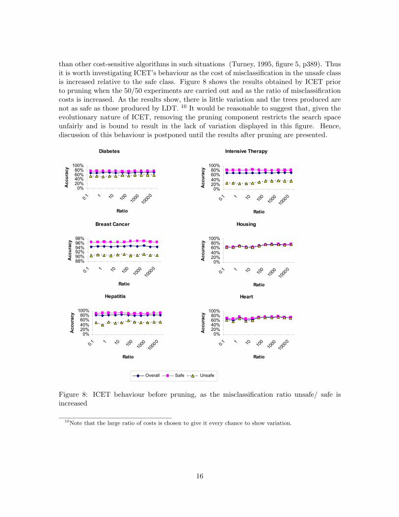
than other cost-sensitive algorithms in such situations (Turney, 1995, figure 5, p389). Thusit is worth investigating ICET’s behaviour as the cost of misclassification in the unsafe classis increased relative to the safe class. Figure 8 shows the results obtained by ICET priorto pruning when the 50/50 experiments are carried out and as the ratio of misclassificationcosts is increased. As the results show, there is little variation and the trees produced arenot as safe as those produced by LDT. 10 It would be reasonable to suggest that, given theevolutionary nature of ICET, removing the pruning component restricts the search spaceunfairly and is bound to result in the lack of variation displayed in this figure. Hence,discussion of this behaviour is postponed until the results after pruning are presented.
Diabetes
0%
20%
40%60%
80%
100%
0.1 1 1
0100
1000
10000
Ratio
Accu
racy
Breast Cancer
88%
90%
92%94%
96%
98%
0.1 1 1
0100
1000
10000
Ratio
Accu
racy
Hepatitis
0%
20%
40%
60%
80%
100%
0.1 1 1
0100
1000
10000
Ratio
Accu
racy
Intensive Therapy
0%
20%
40%
60%
80%
100%
0.1 1 1
0100
1000
10000
Ratio
Accu
racy
Housing
0%
20%
40%
60%
80%
100%
0.1 1 1
0100
1000
10000
Ratio
Accu
racy
Heart
0%
20%
40%
60%
80%
100%
0.1 1 1
0100
1000
10000
Ratio
Accu
racy
Overall Safe Unsafe
Figure 8: ICET behaviour before pruning, as the misclassification ratio unsafe/ safe isincreased
10Note that the large ratio of costs is chosen to give it every chance to show variation.
16

Breast Cancer
86
88
90
92
94
96
98
30/ 70 50/ 50 70/ 30
Training/Testing set
%A
ccu
racy
Diabetes
0
10
20
30
40
50
60
70
80
30/ 70 50/50 70/ 30
Training/Testing set
%A
ccu
racy
Housing
70
75
80
85
90
95
30/ 70 50/ 50 70/ 30
Training/Testing set
%A
ccu
racy
Intensive Therapy
0
10
20
30
40
50
60
30/ 70 50/ 50 70/ 30
Training/Testing set
%A
ccu
racy
Heart
60
65
70
75
80
85
30/ 70 50/50 70/ 30
Training/Testing set
%A
ccu
racy
Hepatitis
0
10
20
30
40
50
60
70
30/ 70 50/ 50 70/ 30
Training/Testing set
%A
ccu
racy
LDT OC1 AP RLP
Figure 9: Summary of accuracy for the unsafe class after pruning
Results after pruning
As mentioned earlier, post-pruning methods can result in improved accuracy, so the aboveexperiments were repeated with pruning. The pruning methods employed were the defaultmethods associated with the systems: OC1 and AP utilize the MCCP method, and LDTis coupled with the safer variation of MCCP described in section 2. Figure 9 presents theresults for the unsafe class, and table 4 gives the results for the 50/50 experiments (thecomplete results are given in appendix A).
The results obtained show that LDT produces significantly safer trees than the othermethods on almost all the datasets. The only dataset where it does not improve the safety ofthe trees relative to the other methods is the breast cancer data, where both LDT and OC1obtain an accuracy of 94.3% for the unsafe class. When comparing overall accuracy, theonly significant difference occurs on the intensive therapy dataset, where the performanceof both OC1 and AP is better than LDT. But since the accuracy on the unsafe class is
17

Data set System Accuracy Tree TimeOverall Safe Unsafe Depth (secs)
Diabetes LDT 69.9±0.8 67.6±1.7 74.6±2.1 15.3±0.8 3.1±0.08OC1 71.4±0.8 80.3±1.8 55.0±3.6 5.1±1.0 167.8±4.25AP 73.8±0.6 84.2±1.5 54.3±2.4 5.0±1.1 1.7±0.03RLP 75.1 ± 0.7 81.4 ± 1.3 63.3 ± 2.1 3.2 ± 0.6 23.0 ± 0.30
Breast Cancer LDT 95.7±0.3 96.5±0.3 94.3±1.0 5.5±0.6 1.0±0.03OC1 94.6±0.5 94.7±0.7 94.3±1.2 1.9±0.3 82.2±5.04AP 94.1±0.5 94.9±0.7 92.6±1.2 3.1±0.5 0.7± 0.02RLP 96.5 ± 0.2 96.9 ± 0.3 95.6 ± 0.6 1.2± 0.2 12.0 ± 0.50
Heart LDT 75.0 ± 1.1 72.8 ± 2.1 78.0 ± 1.5 9.8 ± 0.6 1.2 ± 0.06OC1 75.8 ± 1.2 77.9 ± 2.5 73.6 ± 2.5 2.4 ± 0.5 38.0 ± 1.04AP 74.4 ± 1.1 77.8 ± 2.1 70.7 ± 2.5 3.6 ± 0.7 0.6 ± 0.01RLP 79.3 ± 0.9 82.1 ± 1.5 76.2 ± 1.9 1.8 ± 0.4 6.4 ± 0.18
Hepatitis LDT 79.4 ± 1.4 85.6 ± 1.8 56.2 ± 4.2 5.0 ± 0.4 0.6 ± 0.04OC1 79.3 ± 1.5 85.4 ± 2.1 56.2 ± 4.5 1.6 ± 0.3 18.5 ± 1.48AP 80.2 ± 1.3 89.4 ± 2.1 45.6 ± 6.6 1.8 ± 0.3 0.4 ± 0.02RLP 78.5 ± 1.4 84.9 ± 1.4 54.7 ± 4.4 1.0 ± 0.0 2.9 ± 0.10
Housing LDT 82.7±0.6 76.2±1.8 88.8±1.2 8.5±0.5 2.1±0.07OC1 81.0±1.0 82.0±2.9 80.3±2.0 3.3±0.6 84.7±2.24AP 81.5±0.6 84.1±1.9 79.3±2.0 3.7±0.8 1.3±0.03RLP 85.2 ± 0.6 86.0 ± 1.4 84.5 ± 1.1 2.4 ± 0.6 15.8 ± 0.42
Intensive Therapy LDT 70.0±1.0 76.8±1.3 47.8±2. 9 9.9±0.6 2.6±0.08OC1 74.8±0.9 89.8±2.4 25.1±5.3 2.5±0.6 82.0±3.51AP 75.9±0.9 92.8±1.8 19.2±4.7 3.8±0.9 1.3±0.04RLP 73.8 ± 1 88.5 ± 2.7 25.7 ± 5.9 2.1 ± 0.4 14.9 ± 0.4
Table 4: Results for 50/50 experiments together with 95% confidence interval after pruning
18

significantly poorer than LDT’s performance, such trees are useless in practice. Indeed,the overall accuracy of 74.8% obtained by OC1 masks the information that in more thana quarter of the trials, OC1 produces simple, one node trees, labelled with the safe class,that are 100% accurate on the safe class but 0% accurate on the unsafe class.
A comparison of these results with those obtained without pruning (given in table 3)reveals the effects of pruning. As expected, pruning does improve accuracy in most cases.More interestingly, the use of pruning with OC1 and AP results in improving the accuracyof the unsafe class for just the breast cancer dataset. For the other 3 data sets, the useof pruning with OC1 and AP actually results in a decrease in the accuracy of the unsafeclass. The adoption of the safer MCCP method does improve the accuracy of the unsafeclass, but, this is at the expense of a reduction in the accuracy of the safe class. Althoughthis is reasonable in the context of safety, these results show that pruning methods do notnecessarily result in balanced improvements to the accuracy of all the classes.
Earlier, discussion of ICET’s results prior to pruning (figure 8) was postponed in casethe lack of variation in accuracy was due to the omission of pruning. As the results infigure 10 show, even after pruning is employed, the accuracy does not vary much on eitherclass as the ratio of misclassification costs is increased.
This behaviour is not too surprising when we consider how ICET works. At the bottomlevel (figure 6), it uses C4.5 to generate trees based on the post-pruning parameter CF,and a selection function ICF that has biases Ci and ω. The pruning algorithm adopted isthe error based pruning method that does not directly take account of costs but may beinfluenced indirectly by the parameter CF. Thus the extent to which the trees generated byC4.5 are influenced by costs depends on how well the genetic algorithm learns biases thatrelate to the costs. The results show that in its current form, the genetic algorithm is unableto learn the biases in a way that is sufficient for generating trees that are biased towards aparticular class. Prior to these experiments, this author (as well as Turney (1995), p 390)thought that ICET’s inability to improve the accuracy of the unsafe class was due to thefewer number of examples available relative to the safe class. So it is worth noting that,as the results of the housing data (where each class has approximately 50% of the data)show, ICET’s lack of sensitivity to unbalanced misclassification costs is independent of theproportion of examples available for training from each class.
4 Conclusion and Future Work
This paper has presented a decision tree induction algorithm aimed at domains where safetyis paramount, costs of misclassification are not easy to estimate accurately and where it isknown that the cost of misclassification for one of the classes is significantly higher thananother. The algorithm errs on the side of caution by aiming to avoid concluding that aprocess is safe without supporting examples. To improve the chances of achieving this goalthe algorithm utilises oblique divisions in preference to the less flexible axis-parallel splits.The algorithm, called LDT, utilises the linear discriminant method to identify the initialdivision which is then adapted to favour the development of a tree that errs on the safeside.
An alternative way of tackling the problem could be to utilise an existing cost-sensitivealgorithm and use a high cost for the more costly class. Given the use of oblique splits,
19

Diabetes
0%
20%
40%60%
80%
100%
0.1 1 1
0100
1000
10000
Ratio
Accu
racy
Intensive Therapy
0%
20%
40%60%
80%
100%
0.1 1 1
0100
1000
10000
Ratio
Accu
racy
Breast Cancer
88%
90%
92%94%
96%
98%
0.1 1 1
0100
1000
10000
Ratio
Accu
racy
Housing
0%
20%
40%60%
80%
100%
0.1 1 1
0100
1000
10000
Ratio
Accu
racy
Hepatitis
0%
20%
40%60%
80%
100%
0.1 1 1
0100
1000
10000
Ratio
Accu
racy
Heart
0%
20%
40%60%
80%
100%
0.1 1 1
0100
1000
10000
Ratio
Accu
racy
Overall Safe Unsafe
Figure 10: ICET’s behaviour after pruning, as the misclassification ratio unsafe/safe isincreased
it could also be argued that existing oblique decision tree algorithms may be adequate.Hence, the algorithm is evaluated relative to OC1, the axis parallel approach (AP), RobustLinear Programming (RLP) and an implementation of ICET. Since pruning can have itsown effects on accuracy, experiments were carried out both before and after pruning. Thedefault pruning methods were adopted for OC1, AP, and ICET, while a simple variation ofthe MCCP method that took account of safety was used with LDT. Both before and afterpruning, LDT produces trees that are significantly safer than OC1, AP, RLP and ICET.The only exception occurs on the breast cancer data set after pruning, where OC1 performsas well as LDT, and where, with accuracies of about 95%, there is not much scope forimprovement. Since ICET is an approach that takes account of costs of misclassification,a reasonable proposal for inducing safer trees is to increase the cost of misclassification inthe unsafe class relative to the safe class. Hence experiments, in which the ratio of costs ofmisclassifications was varied were carried out on an implementation of ICET. The resultsrevealed that ICET is not particularly sensitive to imbalanced costs of misclassification and
20

that the trees do not become any safer as the ratio is increased. Further, the experimentsshow that this lack of sensitivity is not simply due to an imbalance in the proportion ofexamples available in the classes as previously thought.
In general, the improvements in safety obtained by LDT are without sacrificing theoverall accuracy. For the diabetes, breast cancer, and housing datasets, the overall accuracyobtained by LDT is similar to that obtained by OC1, both before and after pruning. Forthe intensive therapy data set, the overall accuracy obtained by OC1 and AP is significantlyhigher than that obtained by LDT. However, this is achieved by taking advantage of the lowratio of unsafe cases in the data set to the extent that over a quarter of the trees degenerateinto always returning the safe class. Such degenerate trees are, of course, not much use inany application.
Comparing the results obtained before and after pruning reveals that post-pruning meth-ods can have an unbalanced effect on the accuracy of the classes. The use of the defaultpruning strategies with OC1, AP, and ICET resulted in no significant improvement to thesafety of the trees, while the use of the adapted pruning method improved the safety of thetrees, but with a reduction in the accuracy of the safe class.
There are several areas for further work. In a related study, non-linear divisions havebeen used to develop a cost-sensitive algorithm (Vadera, 2005) but which relies on theavailability of costs. Adapting non-linear divisions for safety applications is likely to bemore difficult but represents a natural extension of this work. Several authors have alsoexperimented with the use of boosting for cost-sensitive problems (Domingos, 1999; Fan,Stolfo, Zhang, & Chan, 1999; Ting, 2000; Merler, Furlanello, Larcher, & Sboner, 2003).Attempts to use boosting coupled with the algorithm presented in this paper also representsa further potential enhancement.
To conclude, this paper has developed a tree induction algorithm that results in safertrees whilst maintaining overall accuracy and which is more appropriate for safety applica-tions.
5 Acknowledgements
The work presented in this paper is a significant development of work that was initiatedwith the help of a Research Assistant, Said Nechab in 1994-95. In particular, the motivationand examples in section 2 appear in a previous joint paper written and presented by theauthor at Knowldege Based Systems Conference in 1996.
The author is grateful to David Ventura for implementing ICET as part of his MScproject, and for the results included in appendix B.
The author is also grateful to Sreerama Murthy for making his OC1 system availableand the anonymous referees for their comments.
References
Althoff, K., Auriol, E., Barletta, R., & Manago, M. (1995). A review of industrial case-basedreasoning tools. Oxford: AI Intelligence.
21

Bennett, K. P. (1999). On mathematical programming methods and support vector ma-chines. In Schoelkopf, A., Burges, C., & Smola, A. (Eds.), Advances in Kernel Methods– Support Vector Machines, chap. 19, pp. 307–326. MIT Press, Cambridge, MA.
Berry, M., & Linoff, G. (2004). Data Mining Techniques (2nd edition). John Wiley.
Blake, C., & Merz, C. (1998). UCI Repository of Machine Learning Databases. [http://www.ics.uci.edu/ mlearn/ MLRepository.html], Irvine, CA: University of California,Department of Information and Computer Science, USA.
Bradford, J., Kunz, C., Kohavi, R., Brunk, C., & Brodley, C. (1998). Pruning decisiontrees with misclassification costs. In Proceedings of the Tenth European Conferenceon Machine Learning, pp. 131–136.
Breiman, L., Friedman, J. H., Olsen, R. A., & Stone, C. J. (1984). Classification andRegression Trees. Belmont: Wadsworth.
Breslow, L., & Aha, D. (1997). Simplifying decision trees: A survey. Knowledge EngineeringReview, 12, 1–40.
Cohen, R. (1995). Empirical Methods for Artificial Intelligence. Massachusetts : MIT Press.
Domingos, P. (1999). MetaCost: A general method for making classifiers cost-sensitive. InProceedings of the Fifth International Conference on Knowledge Discovery and DataMining, pp. 155–164.
Draper, B., Brodley, C. E., & Utgoff, P. E. (1994). Goal-directed classification using lin-ear machine decision trees. IEEE Transactions on Pattern Analysis and MachineIntelligence, 16 (9), 888–893.
Elkan, C. (2001). The foundations of cost-sensitive learning. In Proceedings of the 17thInternational Joint Conference on Artificial Intelligence, pp. 973–978.
Elomaa, T., & Kaariaine, M. (2001). An analysis of reduced error pruning. Journal ofArtificial Intelligence Research, 15, 163–187.
Fan, W., Stolfo, S., Zhang, J., & Chan, P. (1999). AdaCost: Misclassification cost-sensitiveboosting. In Proceedings of the 16th International Conference on Machine Learning,pp. 97–105. Morgan Kaufmann, San Francisco, CA.
Frank, E., & Witten, I. (1998). Reduced-error pruning with significance tests,[http://citeseer.ist.psu.edu/frank98reducederror.html]..
Grefenstette, J. (1986). Optimization of control parameters for genetic algorithms. IEEETransactions on Systems, Man, and Cybernetics, 16, 122–128.
Knoll, U., Nakhaeizadeh, G., & Tausend, B. (1994). Cost-sensitive pruning of decisiontrees. In Proceedings of the Eight European Conference on Machine Learning, Vol. 2,pp. 383–386, Berlin, Germany. Springer-Verlag.
Kolodner, J. (1993). Case-based Reasoning. Palo Also, CA:Morgan Kaufman.
Martin, A., Doddington, G., Kamm, T., Ordowski, M., & Przybocki, M. (1997). The DETcurve in assessment of detection task performance. In Proceedings of Eurospeech ’97,pp. 1895–1898, Rhodes, Greece.
22

Merler, S., Furlanello, C., Larcher, B., & Sboner, A. (2003). Automatic model selection incost-sensitive boosting. Information Fusion, 4, 3–10.
Mingers, J. (1989). An empirical comparison of pruning methods for decision tree induction.Machine Learning, 4, 227–243.
Morrison, D. (1976). Multivariate Statistical Methods (Second edition). New York :McGraw-Hill.
Murthy, S., Kasif, S., & Salzberg, S. (1994). A system for induction of oblique decisiontrees. Journal of Artificial Intelligence Research, 2, 1–32.
Norusis, M. (1994). SPSS Advanced Statistics 6.1. SPSS Inc., Chicago, Illinois 60611, USA.
Nunez, M. (1991). The use of background knowledge in decision tree induction. MachineLearning, 6, 231–250.
Pazzani, M., Merz, C., Murphy, P., Ali, K., Hurne, T., & Brunk, C. (1994). Reducingmisclassification costs: Knowledge-intensive approaches to learning from noisy data.In Proceedings of the Eleventh International Conference on Machine Learning, pp.217–225.
Provost, F. J., & Buchanan, B. G. (1995). Inductive policy: The pragmatics of bias selection.Machine Learning, 20, 35–61.
Provost, F. J., Fawcett, T., & Kohavi, R. (1998). The case against accuracy estimationfor comparing induction algorithms. In Proceedings of the Fifteenth InternationalConference on Machine Learning, pp. 445–553.
Quinlan, J. R. (1987). Simplifying decision trees. International Journal of Man-MacineStudies, 27, 221–234.
Quinlan, J. R. (1993). C4.5 : Programs for Machine Learning. California:Morgan Kauffman.
Tan, M. (1993). Cost-sensitive learning of classification knowledge and its applications inrobotics. Machine Learning, 13, 7–33.
Ting, K. (2000). A comparative study of cost-sensitive boosting algorithms. In Proceedingsof the 17th International Conference on Machine Learning, pp. 983–990.
Turney, P. (1995). Cost sensitive classification: Empirical evaluation of a hybrid geneticdecision tree induction algorithm. Journal of Artificial Intelligence Research, 2, 369–409.
Vadera, S. (2005). Inducing Cost-Sensitive Nonlinear Decision Trees, Technical Report.School of Computing, Science and Engineering, University of Salford, Salford, M54WT, UK, [http://citeseer.ist.psu.edu].
Vadera, S., & Ventura, D. (2001). A comparison of cost-sensitive decision tree learning algo-rithms. In Proceedings of the Second European Conference on Intelligent ManagementSystems in Operations, pp. 79–86.
Vanderbe, R. (2002). Loqo: Optimisation and Applications Web Site. Princeton University,NJ 08544, [http://orfe.princeton.edu/ loqo/].
Zadrozny, B., Langford, J., & Abe, N. (2003). A simple method for cost-sensitive learning.IBM Technical Report RC22666, [http://citeseer.ist.psu.edu/zadrozny03simple.html].
23

A Results of Empirical Evaluations of LDT, AP, RLP andOC1
This appendix presents the complete set of results for LDT, AP,RLP and OC1 both beforeand after pruning. The experimental method used is described in the body of the paper.
Diabetes (unpruned)Train/Test System Accuracy Safe Unsafe Depth Time (s)
30/70 LDT 68.1±1.6 73.1±1.2 58.9±2.0 13.3±0.5 1.7±0.05OC1 67.7±0.8 75.2±1.2 54.0±1.6 9.4±0.4 92.0±2.46AP 68.5±1.0 76.0±1.1 54.8±1.9 12.2±0.5 1.0±0.02RLP 66.9 ± 0.7 71.8 ± 1.1 58.0 ± 1.7 38.4 ± 5.4 13.60 ± 0.20
50/50 LDT 69.4±1.5 73.8±0.9 61.3±1.4 17.1±0.7 3.3±0.09OC1 68.5±1.2 75.5±1.0 55.4±1.6 11.2±0.3 192.3±5.10AP 69.7±1.1 76.4±0.9 57.2±1.4 14.2±0.4 1.8±0.03RLP 67.4 ± 0.7 72.5 ± 1.1 57.9 ± 1.5 46.0 ± 3.8 27.3 ± 0.31
70/30 LDT 68.7±2.2 73.8±1.0 59.5±1.8 19.1±0.6 5.0±0.08OC1 68.4±1.3 75.8±1.1 55.1±1.7 12.7±0.4 313.0±9.60AP 69.6±1.4 77.5±1.0 55.3±1.6 15.4±0.5 2.7±0.05RLP 68.0 ± 0.8 74.0 ± 1.1 57.1 ± 1.5 46.9 ± 3.3 42.8 ± 0.30
Breast Cancer (unpruned)Train/Test System Accuracy Safe Unsafe Depth Time (s)
30/70 LDT 94.9±0.8 96.4±0.3 92.0±0.9 5.5±0.3 0.6±0.03OC1 93.6±0.5 95.8±0.5 89.5±1.4 4.4±0.3 43.0±2.09AP 93.9±0.7 95.6±0.4 90.8±0.8 6.2±0.5 0.3±0.01RLP 93.9 ± 0.4 96.2±0.37 89.64 ± 1.41 4.6 ± 2.7 6.3 ± 0.40
50/50 LDT 95.1±1.0 96.4±0.3 92.6±1.1 7.1±0.4 1.1±0.03OC1 94.3±0.5 96.4±0.3 90.4±1.2 6.3±0.3 91.5±7.27AP 94.5±0.8 96.4±0.4 90.8±1.0 7.7±0.4 0.7±0.02RLP 94.8± 0.4 96.4 ± 0.3 91.9± 1.2 16.5±5.1 13.8±0.52
70/30 LDT 95.1±1.0 96.7±0.4 92.2±1.2 8.3±0.4 1.8±0.05OC1 94.5±0.7 96.3±0.4 91.0±1.0 6.8±0.3 145.2±6.77AP 94.6±0.8 96.2±0.5 91.7±1.0 8.7±0.4 1.2±0.04RLP 93.5± 0.5 95.8± 0.4 89.2 ±1.5 14.6 ± 4.5 23.4 ± 0.60
24

Heart(unpruned)Train/Test System Accuracy Safe Unsafe Depth Time (s)
30/70 LDT 73.8 ± 1.0 74.0 ± 1.8 73.9 ± 2.3 7.5± 0.5 0.6± 0.03OC1 73.1 ± 0.9 73.8 ± 2.0 72.5 ± 1.9 5.6± 0.4 19.9± 0.76AP 72.9 ± 1.0 75.9 ± 1.6 69.6 ± 2.5 6.7± 0.4 0.4± 0.01RLP 72.8 ± 1.0 74.9 ± 1.6 70.7 ± 2.2 9.0± 4.0 3.8± 0.15
50/50 LDT 74.1 ± 1.1 73.9 ± 1.9 74.7 ± 1.6 9.8± 0.5 1.3± 0.05OC1 74.0 ± 1.0 74.4 ± 1.7 73.9 ± 1.7 6.8± 0.3 44.8± 1.26AP 72.9 ± 0.9 74.4 ± 1.7 71.3 ± 1.6 7.8± 0.3 0.7± 0.02RLP 76.1 ± 1.1 77.8 ± 2.2 74.6 ± 1.7 26.6± 6.1 7.4± 0.25
70/30 LDT 73.6 ± 1.2 72.0 ± 1.9 75.2 ± 2.0 11.2± 0.5 2.1± 0.07OC1 74.8 ± 1.3 75.6 ± 2.1 74.2 ± 1.9 7.6± 0.3 75.3± 2.18AP 73.4 ± 1.3 75.1 ± 2.0 71.6 ± 1.7 9.2± 0.5 1.1 ±0.02RLP 74.1 ± 1.2 74.4 ± 2.3 74.1 ± 2.3 33.3± 5.8 12.2± 0.31
Hepatitis(unpruned)Train/Test System Accuracy Safe Unsafe Depth Time (s)
30/70 LDT 79.6 ± 1.3 86.0 ± 1.8 55.9 ± 3.7 3.0 ± 0.4 0.3 ± 0.0OC1 80.0 ± 1.2 87.3 ± 1.8 53.3 ± 4.4 3.2 ± 0.3 8.6 ± 0.6AP 79.7 ± 1.1 87.4 ± 1.5 50.5 ± 3.9 4.1 ± 0.3 0.2 ± 0.0RLP 77.1 ± 1.6 83.4 ± 1.8 54.3 ± 4.2 1.1 ± 0.1 1.6 ± 0.0
50/50 LDT 80.5 ± 1.1 87.0 ± 1.5 56.0 ± 3.6 5.1 ± 0.4 0.7 ± 0.1OC1 80.7 ± 1.5 87.4 ± 1.6 54.6 ± 4.4 4.7 ± 0.4 22.1 ± 1.7AP 80.0 ± 1.5 87.1 ± 1.7 52.7 ± 3.9 5.6 ± 0.4 0.4 ± 0.0RLP 79.4 ± 1.3 86.1 ± 1.4 53.3 ± 4.2 4.8 ± 3.3 3.4 ± 0.1
70/30 LDT 80.9 ± 1.7 86.9 ± 1.9 58.4 ± 4.5 7.1 ± 0.5 1.4 ± 0.1OC1 82.9 ± 1.5 89.5 ± 1.7 57.4 ± 4.9 5.5 ± 0.3 38.3 ± 2.0AP 81.9 ± 1.4 88.0 ± 1.8 59.6 ± 4.2 6.4 ± 0.4 0.6 ± 0.0RLP 80.1 ± 1.4 87.4 ± 1.6 52.5 ± 4.5 13.2 ± 5.0 5.9 ± 0.4
25

Housing (unpruned)Train/Test System Accuracy Safe Unsafe Depth Time (s)
30/70 LDT 82.8±1.0 81.3±1.5 84.3±1.0 7.9±0.5 1.1±0.04OC1 80.9±0.5 80.8±1.4 81.1±1.1 6.6±0.3 45.5±1.31AP 80.9±0.7 80.2±1.3 81.6±1.1 8.1±0.4 0.7±0.02RLP 82.3 ± 0.6 82.3 ± 1.3 82.4 ± 1.1 18.1± 5.8 9.2 ± 0.18
50/50 LDT 83.3±1.2 81.3±1.3 85.2±1.1 10.2±0.5 2.3±0.07OC1 82.4±0.8 82.3±1.2 82.6±1.2 7.7±0.3 104.6±4.41AP 81.7±0.8 81.3±1.2 82.1±1.1 9.2±0.4 1.4±0.03RLP 83.1 ± 0.5 81.2 ± 1.2 85.0 ± 1.1 25.3 ± 5.9 18.3 ± 0.40
70/30 LDT 83.4±1.3 81.1±1.4 85.6±1.0 11.4±0.5 3.6±0.09OC1 82.3±0.8 82.4±1.3 82.3±1.1 9.0±0.3 164.5±4.10AP 82.6±0.8 82.8±1.5 82.6±1.2 11.0±0.4 2.3±0.04RLP 83.2 ± 0.7 80.5 ± 1.6 85.7 ± 1.1 34.2 ± 5.8 30.1 ± 0.56
Intensive Therapy (unpruned)Train/Test System Accuracy Safe Unsafe Depth Time (s)
30/70 LDT 70.0±0.9 77.7±1.3 44.3±2.4 8.9±0.5 1.5±0.07OC1 72.1±0.5 82.1±1.3 38.7±2.2 6.6±0.3 42.2±2.50AP 71.5±0.7 81.5±1.4 38.1±2.0 7.9±0.4 0.7±0.03RLP 69.5 ± 0.8 78.6 ± 1.4 39.1 ± 2.6 20.2± 5.9 8.3 ± 0.27
50/50 LDT 70.4±1.0 78.2±1.3 44.2±2.4 11.2±0.5 3.0±0.09OC1 72.5±0.6 83.0±1.0 37.8±2.8 8.2±0.4 99.1±2.87AP 72.2±0.7 81.9±1.0 39.7±2.3 9.7±0.4 1.4±0.04RLP 70.5 ± 1.0 80.6 ± 1.4 37.2 ± 2.4 25.0 ± 5.9 17.3 ± 0.46
70/30 LDT 71.4±0.9 79.1±1.2 45.3±3.2 12.4±0.5 4.4±0.11OC1 71.3±0.8 81.0±1.1 38.5±3.1 9.3±0.4 169.5±4.35AP 72.0±0.8 81.5±1.2 39.6±3.3 11.0±0.5 2.2±0.05RLP 70.1 ± 1.2 79.0 ± 1.5 39.7 ± 3.4 40.2 ± 5.1 29.4± 0.49
26

Diabetes (pruned)Train/Test System Accuracy Safe Unsafe Depth Time (s)
30/70 LDT 68.8±0.8 67.9±2.1 70.8±2.8 11.8±0.8 1.6±0.04OC1 70.6±0.7 79.5±2.7 54.2±5.1 3.4±0.7 79.0±2.16AP 71.7±0.7 82.5±2.4 52.0±3.5 4.9±1.1 0.9±0.02RLP 74±0.54 80.82± 1.76 61.52 ± 3.12 4.78 ± 1.73 10.2 ± 0.47
50/50 LDT 69.9±0.8 67.6±1.7 74.6±2.1 15.3±0.8 3.1±0.08OC1 71.4±0.8 80.3±1.8 55.0±3.6 5.1±1.0 167.8±4.25AP 73.8±0.6 84.2±1.5 54.3±2.4 5.0±1.1 1.7±0.03RLP 75.1 ± 0.7 81.4 ± 1.3 63.3 ± 2.1 3.2 ± 0.6 23.0 ± 0.30
70/30 LDT 69.9±0.8 67.6±1.7 74.6±2.1 15.3±0.8 3.1±0.08OC1 71.7±0.9 79.9±2.1 56.6±3.3 5.2±0.9 276.5±6.98AP 73.6±0.8 85.1±1.6 52.8±2.5 5.9±1.3 2.6±0.05RLP 74.5 ± 0.9 81.9 ± 1.5 60.9 ± 2.8 3.1 ± 0.6 37.5 ± 0.37
Breast Cancer (pruned)Train/Test System Accuracy Safe Unsafe Depth Time (s)
30/70 LDT 95.8±0.5 96.0±0.5 95.3±1.2 5.5±0.9 1.6±0.05OC1 94.0±0.4 93.8±0.8 94.3±0.8 1.3±0.2 36.1±1.95AP 92.7±0.5 93.7±0.9 90.8±1.8 2.2±0.4 0.3±0.02RLP 95.5 ± 0.4 96.3 ± 0.4 93.8 ± 1.0 5.1 ± 0.3 5.1 ± 0.30
50/50 LDT 95.7±0.3 96.5±0.3 94.3±1.0 5.5±0.6 1.0±0.03OC1 94.6±0.5 94.7±0.7 94.3±1.2 1.9±0.3 82.2±5.04AP 94.1±0.5 94.9±0.7 92.6±1.2 3.1±0.5 0.7± 0.02RLP 96.5 ± 0.2 96.9± 0.3 95.6± 0.6 1.2± 0.2 12.0± 0.50
70/30 LDT 95.8±0.5 96.0±0.5 95.3±1.2 5.5±0.9 1.6± 0.05OC1 95.4±0.4 95.6±0.6 95.2±1.0 2.2±0.5 123.4±5.88AP 94.4±0.5 95.4±0.7 92.8±1.2 3.9±0.6 1.1±0.04RLP 96.4 ± 0.4 96.6 ± 0.5 96.6 ± 0.5 2.5 ± 2.0 9.8±0.60
27

Heart(pruned)Train/Test System Accuracy Safe Unsafe Depth Time (s)
30/70 LDT 74.0 ± 1.0 72.7 ± 2.5 75.8 ± 2.1 7.2 ± 0.7 0.6 ± 0.05OC1 74.3 ± 1.3 75.9 ± 3.2 72.6 ± 3.0 1.4 ± 0.2 18.0 ± 0.66AP 73.9 ± 0.9 78.1 ± 2.0 69.1 ± 2.6 2.3 ± 0.5 0.3 ± 0.01RLP 78.3 ± 1.0 80.1 ± 1.6 76.1 ± 1.9 1.1 ± 0.1 3.4 ± 0.13
50/50 LDT 75.0 ± 1.1 72.8 ± 2.1 78.0 ± 1.5 9.8 ± 0.6 1.2 ± 0.06OC1 75.8 ± 1.2 77.9 ± 2.5 73.6 ± 2.5 2.4 ± 0.5 38.0 ± 1.04AP 74.4 ± 1.1 77.8 ± 2.1 70.7 ± 2.5 3.6 ± 0.7 0.6 ± 0.01RLP 79.3 ± 0.9 82.1 ± 1.5 76.2 ± 1.9 1.8 ± 0.4 6.4 ± 0.18
70/30 LDT 75.4 ± 1.4 70.1 ± 2.2 81.7 ± 1.8 11.0 ± 0.6 1.9 ± 0.07OC1 75.4 ± 1.3 78.0 ± 2.6 72.6 ± 2.8 2.8 ± 0.5 62.7 ± 1.59AP 75.7 ± 1.4 79.1 ± 2.2 71.8 ± 2.4 3.7 ± 0.7 1.0 ± 0.02RLP 79.9 ± 1.2 82.0 ± 1.9 77.7 ± 1.8 2.2 ± 0.6 10.4 ± 0.29
Hepatitis(pruned)Train/Test System Accuracy Safe Unsafe Depth Time (s)
30/70 LDT 78.8 ± 1.4 85.4 ± 2.0 54.5 ± 4.0 2.3 ± 0.4 0.2 ± 0.01OC1 78.5 ± 1.3 85.9 ± 2.2 50.8 ± 5.4 1.2 ± 0.2 7.2 ± 0.53AP 78.2 ± 1.3 87.5 ± 2.5 44.3 ± 6.5 1.3 ± 0.2 0.2 ± 0.01RLP 76.6 ± 1.4 83.3 ± 1.7 52.4 ± 4.3 1.0 ± 0.0 1.7 ± 0.03
50/50 LDT 79.4 ± 1.4 85.6 ± 1.8 56.2 ± 4.2 5.0 ± 0.4 0.6 ± 0.04OC1 79.3 ± 1.5 85.4 ± 2.1 56.2 ± 4.5 1.6 ± 0.3 18.5 ± 1.48AP 80.2 ± 1.3 89.4 ± 2.1 45.6 ± 6.6 1.8 ± 0.3 0.4 ± 0.02RLP 78.5 ± 1.4 84.9 ± 1.4 54.7 ± 4.4 1.0 ± 0.0 2.9 ± 0.10
70/30 LDT 81.7 ± 1.3 87.1 ± 1.8 61.9 ± 4.2 6.5 ± 0.5 1.2 ± 0.08OC1 82.4 ± 1.5 88.8 ± 1.9 58.2 ± 5.1 1.6 ± 0.3 31.4 ± 2.13AP 82.3 ± 1.7 91.9 ± 1.7 47.1 ± 6.7 2.7 ± 0.5 0.6 ± 0.03RLP 80.3 ± 1.5 86.0 ± 1.8 59.7 ± 4.6 2.3 ± 2.0 5.3 ± 0.30
28

Housing (pruned)Train/Test System Accuracy Safe Unsafe Depth Time (s)
30/70 LDT 81.9±0.6 76.9±1.5 86.6±1.1 7.2±0.7 1.1±0.04OC1 80.9±0.6 82.6±1.8 79.2±1.9 2.8±0.6 38.2±1.55AP 81.0±0.6 83.4±2.5 78.8±2.3 2.9±0.7 0.6±0.02RLP 84.1± 0.7 84.4 ± 5.8 83.8 ± 4.5 1.5 ± 1.0 8.3 ± 0.14
50/50 LDT 82.7±0.6 76.2±1.8 88.8±1.2 8.5±0.5 2.1±0.07OC1 81.0±1.0 82.0±2.9 80.3±2.0 3.3±0.6 84.7±2.24AP 81.5±0.6 84.1±1.9 79.3±2.0 3.7±0.8 1.3±0.03RLP 85.2 ± 0.6 86.0±1.4 84.5 ± 1.1 2.4±0.6 15.8 ± 0.42
70/30 LDT 82.1±1.9 71.9±4.5 91.5±1.4 8.9±0.7 3.2±0.11OC1 82.3±1.1 82.4±2.3 82.4±1.6 4.3±0.7 146.6±5.64AP 81.6±0.8 84.4±1.7 79.3±1.7 5.4±1.1 2.1±0.05RLP 85.1 ± 0.8 85.3 ± 1.5 85.0 ± 1.3 3.2 ± 0.7 26.2 ± 0.60
Intensive Therapy (pruned)Train/Test System Accuracy Safe Unsafe Depth Time (s)
30/70 LDT 70.2±0.9 77.7±1.6 45.0±2.9 8.6±0.5 1.4±0.08OC1 74.7±0.8 88.8±2.4 27.6±5.5 2.2±0.4 36.5±2.08AP 75.3±0.7 93.9±2.0 13.3±4.2 1.7±0.4 0.7±0.03RLP 72.4 ± 1.1 84.7 ± 3.2 31.9 ± 6.4 1.7 ± 0.3 7.1 ± 0.26
50/50 LDT 70.0±1.0 76.8±1.3 47.8±2.9 9.9±0.6 2.6±0.08OC1 74.8±0.9 89.8±2.4 25.1±5.3 2.5±0.6 82.0±3.51AP 75.9±0.9 92.8±1.8 19.2±4.7 3.8±0.9 1.3±0.04RLP 73.8 ± 1 88.5 ± 2.7 25.7 ± 5.9 2.1 ± 0.4 14.9 ± 0.4
70/30 LDT 69.4±1.2 75.3±1.7 49.6±3.2 11.3±0.5 3.8±0.09OC1 75.1±1.1 91.0±2.3 21.4±5.2 3.4±0.8 142.5±4.30AP 76.4±1.0 93.4±1.9 18.7±5.2 3.7±0.9 2.0±0.05RLP 74.1 ± 1.4 91.3 ± 2.7 15.8 ± 5.0 2.2 ± 0.4 25.2 ± 0.53
29

B Repeated Experiments using Re-implementation of ICET
Figure 11 shows the results obtained by both the implementation of ICET utilized in thispaper and the published results in (Turney, 1995, figure 3). The results give confidence thatthe implementation is a fair and accurate representation of ICET. The measure ’Average% Standard Cost’ labelling the Y axis is a normalized average cost of classification. Thismeasure and details of the experimental method are as presented in Turney (1995).
ICET results from Turney (1995).
Results from implementation used in the paper.
Diabetes
0
20
40
60
80
100
10 100 1000 10000
Misclassification Costs
Av.
% S
tand
ard
Cos
t
Bupa Liver Disease
0
20
40
60
80
100
10 100 1000 10000
Misclassification Costs
Av.
% S
tand
ard
Cos
t
Thyroid Disease
0
20
40
60
80
100
10 100 1000 10000
Misclassification Costs
Av.
% S
tand
ard
Cos
t
Figure 11: Published results and those obtained by the implementation of ICET used inthis paper
30