INDUCING LABOR:

EXPERIMENTAL EVIDENCE ON EARLY LIFECYCLE WORK AND FAMILY

TRANSITIONS IN INDIA*

Robert Jensen

Department of Public Policy

UCLA

Abstract: Do labor market opportunities for women affect marriage and fertility decisions? We provided

three years of recruiting services to help young women in randomly selected rural Indian villages get jobs

in the business process outsourcing industry. Because the industry was so new at the time of the study,

there was almost no awareness of these jobs, allowing us to in effect exogenously increase women's labor

force opportunities from the perspective of rural households. We find that young women in treatment

villages were significantly less likely to get married or have children during this period, choosing instead

to enter the labor market or obtain more schooling or post-school training. Women also report wanting to

have fewer children and to work more steadily throughout their lifetime, consistent with increased

aspirations for a career.

* I would like to thank Dora Costa, Pascaline Dupas, Nolan Miller, Adriana Lleras-Muney, Mai Nguyen,

Jeff Nugent, Emily Oster, Paul Gertler, John Strauss and seminar participants at Berkeley, Columbia, the

University of Chicago and Yale for valuable comments and discussions. Financial support from the

Center for Aging and Health Research at the National Bureau of Economic Research, the Women and

Public Policy Program, the Dean's Research Fund at and the William F. Milton Fund at Harvard

University is gratefully acknowledged. I would also like to thank Shubhashis Gangopadhyay and the

India Development Foundation for hosting me during the initial stages of this project. This paper replaces

"Economic Opportunities and Gender Differences in Human Capital: Experimental Evidence from India,"

NBER Working Paper No. 16021.

1

I. INTRODUCTION

In many developing countries, women frequently leave school, marry and start having

children at a young age. Such outcomes are often taken as indicators of low social and economic

progress for women, and may have implications for individual well-being and economic growth.

Economic models suggest that the labor market may play a role in influencing these outcomes.

Because childrearing is traditionally more intensive in women's time, when there are few well-

paying opportunities for women, the opportunity cost of having many children, or getting

married and having children at a young age rather than accumulating human capital and/or

entering the labor market, is low (e.g., Becker 1960, Mincer 1963, Willis 1973). In this paper, we

test whether an exogenous increase in employment opportunities for women can affect these

early lifecycle work and family transitions in rural India.

Rural India is a valuable setting for testing this hypothesis. Among rural women aged 30

to 39 in 2005/6, the median age at marriage was 17 and the median of age at first birth was 19;

and though there have been large declines in the past few decades, women aged 40 to 49 had 4.3

births on average in their lifetime (IIPS and Macro International 2007). Alongside these

outcomes, women's paid labor force participation rates are only around 20 percent.

In order to examine the effect of an exogenous change in labor market opportunities for

women, we conducted a randomized trial using recruiters for the Business Process Outsourcing

(BPO) industry. This industry has grown rapidly in India over the past decade, creating a

significant number of new, high-paying job opportunities, particularly for women. However,

because it was such a new sector, awareness of these jobs and knowledge of how to access them

was very limited, especially outside of the urban areas where these jobs were located. Our

intervention provided three years of BPO recruiting services to women in randomly selected

rural villages. By connecting the villages to experienced recruiters, the intervention was designed

to increase awareness of and access to BPO jobs, and thus in effect increase employment

opportunities for women. Randomization allows us to overcome concerns about omitted

variables bias and the fact that women's labor force participation, human capital, marriage and

fertility decisions are likely to be jointly determined, which often makes it difficult to untangle

the isolated, causal impact of a single factor.

As in many other developing countries, although women's paid labor force participation

rates are low in rural India, they are in fact very economically active. However, most women

2

work in household production or on their own family farm or enterprise. For human capital,

marriage and fertility decisions, the kinds of opportunities available to and actually engaged in

by women can be important. For example, work around the home or on a family enterprise may

not require delays in marriage or fertility to the same extent, nor does it typically require the

same investment in human capital. And self-employment profits are generally quite low,

implying a low opportunity cost to withdrawing from work in order to have children.

A number of factors may explain why fewer women work away from home for pay, such

as a low capital-to-labor ratio that makes production more intensive in physical than mental tasks

(favoring men's comparative advantage) or a social stigma against women working outside the

home (Goldin 1990). But technological change may create jobs that require (and reward) greater

human capital, favor women's comparative advantage, and do not carry as much of a stigma for

women. In this spirit, Goldin (1995) describes a U-shaped pattern in women's labor force

participation. At low levels of economic development, women have high employment rates,

primarily in agriculture or self-employment. As incomes rise, women leave the labor market, in

part because of a preference that women not work outside the home in manual labor. But with

greater development, and increases in women's human capital, white collar opportunities become

available and draw women back into the labor force.1 The BPO sector is an example of this kind

of change, and represents a particularly relevant case study given the historical role of similar

jobs, including those fostered by new office and information technologies, in increasing women's

labor force participation (Goldin 1984, 1990, 1995, 2006).

Using panel data spanning a three year period, we find that women aged 15 to 21 at

baseline from villages exposed to the recruiting intervention were 4.6 percentage points more

likely to work in a BPO job than women in control villages, and 2.4 percentage points more

likely to work at all for pay outside the home. In addition, women from treatment villages

expressed a greater interest in working throughout their lives, even after marriage and childbirth,

indicating shifting aspirations towards work as a career with a longer-term attachment.

The higher educational requirements and greater returns to human capital in the BPO

sector also led to increased investments for women. The cohort of 15 to 21 year old women from

treatment villages were significantly more likely enroll in computer or English language courses

at private, for-fee training institutes, indicating a willingness to invest towards getting a job or

1 See also Boserup (1970), Costa (2000), Schultz (1990) and Mammen and Paxson (2000).

3

building a career when suitable opportunities are available. Younger, school-aged girls stayed in

school longer and had greater Body Mass Index (BMI), reflecting better nutrition and/or health

investments. These gains are particularly significant in light of the dramatic gender disparities in

health and education in India (see Strauss and Thomas 1995, Behrman 1997 and Duflo 2005).

Finally, the increases in women's employment and schooling/training were accompanied

by significant delays in marriage and childbearing. Women from treatment villages aged 15 to 21

at baseline, the peak age range for marriage and the initiation of childbearing in rural India, were

5 to 6 percentage points less likely to get married or to have given birth over the three year

period of our intervention. And though with a short panel we cannot assess the long-term impact

on fertility, women report wanting to have 0.35 fewer children in their lifetime.

Of course, we would not claim that labor market opportunities for women are the only

means to simultaneous human capital, marriage and fertility change.2 For example, Duflo, Dupas

and Kremer (2011) find that lowering the costs of schooling (via free uniforms) increases

education and reduces teen marriage and pregnancy in Kenya. For the U.S., Goldin and Katz

(2000, 2002) find that by lowering the cost of investing in careers and delaying marriage, the oral

contraceptive pill led to increases in women's human capital investments, delayed marriage and

lower desired fertility; Bailey (2006) finds that it also led to increases in women's labor force

participation and delays in actual fertility. However, our results do imply that economic or labor

market factors can have significant effects on marriage, fertility and human capital investments,

and that policies that promote labor market opportunities for women may help improve these

outcomes. By contrast, many policies designed to address these outcomes have primarily

emphasized the role of social or cultural influences or factors (see Croll 2000 for examples).

The remainder of this paper proceeds as follows. Section II discusses the experimental

design and Section III discusses the data and empirical strategy. Section IV shows the results,

and Section V provides a series of tests to determine whether mechanisms other than economic

opportunities for younger women can explain the results. Section VI concludes.

2 Or for that matter, that only white collar jobs affect women's marriage and fertility outcomes. For

example, Schultz (1985) finds that increases in the female-to-male relative wage rate driven by world

price changes for male-intensive food crops and female-intensive dairy products contributed to fertility

decline in Sweden in the late 19th and early 20th centuries.

4

II. EXPERIMENTAL DESIGN

II. A. The BPO Sector in India

The Business Process Outsourcing (BPO) industry covers a range of activities and "back

office" services. The most well-known of these jobs are call centers, but the sector also includes

data entry and management, claims processing, secretarial services, transcription and online

technical support, as well as more skilled activities such as accounting or software development.

Though the industry has been around in some form for decades, recent technological changes in

telecommunications and networking infrastructure (for example, the development and global

deployment of fiber optic cable networks) have made it both possible and relatively inexpensive

to provide these services remotely to clients around the world. And in recent decades, India has

enacted regulatory changes allowing greater foreign investment in the telecommunications

sector. The technological and regulatory changes led to large scale and rapid growth in India's

BPO sector, with 30−40% average annual growth rates from 2000 to 2008 (NASSCOM 2009).

Within the BPO sector, particularly call centers, there appears to be a preference for

female workers. A study of 2,500 call centers in 17 countries found that on average, 69% of

frontline call center workers are women (Holman, Batt and Holtgrewe 2007). Though the rate

was closer to 45% in India, this is still high in comparison to the sex ratio of employment in most

other industries. The study reported several reasons employers preferred women, including a

more pleasant voice and demeanor when interacting with customers, and the belief that women

were more trustworthy than men.

BPO jobs on average have high educational requirements, typically a minimum of 10 or

12 years of schooling. Below, we show that this exceeds the average attainment levels for both

men and women in our rural sample.

Overall then, growth in the BPO sector in India created a sharp and fairly sudden increase

in the demand for educated female workers. In order to meet this demand, there was a surge in

recruiting activities, including through newly-formed, specialized private contractors and

subcontractors who would seek out and screen potential employees. And because the BPO sector

in India is strongly geographically concentrated, with 95% of employment focused around seven

major cities, recruiting was fairly geographically concentrated as well, leading to large, localized

increases in economic opportunities.

5

BPO jobs are also well-paid in relative terms. In our data, starting salaries with no

experience often ranged from 5,000−10,000 Rupees (about $U.S. 110−220) per month in 2003.

This was twice the average pay for non-BPO workers with similar levels of education. Salaries

also often increase rapidly with experience, whereas many other jobs have relatively flat

compensation profiles. Accordingly, as in the present paper, Oster and Millett (2010) treat the

growth in call centers as a shock to the returns to education. Shastry (forthcoming) treats the

broader information technology sector in India as a similar shock.

II. B. The Intervention

Though the BPO sector created a large number of employment opportunities for women,

there remained significant gaps in awareness about those jobs and how to access them, precisely

because the industry was so new. This was even more pronounced outside the urban centers

where these jobs were located; in fact, in our 2003 baseline survey of rural households described

below, no one was employed in this sector, including any members or children of members

having temporarily or permanently left the household. Our experiment was designed to both

increase awareness of these jobs3 and to make it easier for qualified women to get them.

We hired eight BPO recruiters, all with at least two years experience overall and at least

six months specifically recruiting women (either working directly for recruiting firms or as

freelancers). We drew the recruiters from Delhi, one of the most important cities for the BPO

sector. Using maps, the recruiters were asked to identify the specific areas within and outside of

Delhi they had visited for recruiting, and then to define the approximate areas outside of Delhi

beyond which they believed BPO recruiters would be unlikely to visit, due solely to their relative

distance from the city and/or their population size. This allowed us to establish a list of rural

districts where awareness of and access to BPO jobs was likely to be low, not because there were

no qualified women, but simply because the cost per potential recruit was high enough that

recruiters chose to visit other areas instead. These districts were all located approximately

50−150km from Delhi, in the states of Haryana, Punjab, Rajasthan and Uttar Pradesh (see

Appendix Figure 1). These villages are on average closer to Delhi than the average village in

rural India is to the nearest major urban center, more populous (1,900 people on average,

3 In this respect, the experiment is similar to Jensen (2010), who examines the effect of providing

information on the returns to schooling on male educational attainment the Dominican Republic.

6

compared to around 1,200 for all of rural India) and have better infrastructure. We would

therefore not generalize our analysis to all of rural India. There may for example be less of a

response to this kind of opportunity in more remote areas due to differences in factors such as the

openness to women working away from home, poorer quality schools or other infrastructure, or

because being closer to Delhi means that women can commute rather than having to migrate.

We compiled a list of all villages in these districts and randomly assigned 80 villages to

the treatment group and 80 villages to the control group using a random number generator in

Stata, with no additional stratification. We then randomly assigned one of the eight recruiters to

each of the treatment villages, again using the random number generator in Stata. Adherence to

the randomization design was complete; there was no replacement or substitution of villages in

either group, and no replacement or substitution of recruiters across treatment villages.

Between December 2003 and February 2004, recruiters would visit the treatment villages

and make a small introduction at schools and to local leaders, announcing that they would be

visiting the village at a designated date up to a few weeks later to provide information on

employment opportunities in the BPO sector. They also contacted and worked with local leaders,

government officials and NGOs to advertise the sessions.

Within a few weeks, the recruiters would visit the village and set up an information and

recruiting session. The recruiters did not have a fixed script, but were required to follow a

specific organization: an overview of the BPO sector, including the types of jobs and level of

compensation; information on the names of specific firms currently or frequently looking for

workers; strategies for how to apply for jobs (how to create and submit resumes, plus lists of

websites and phone numbers); interview skills lessons and tips; mock interviews; assessment of

English language skills; and a question and answer session. The recruiters were required to

emphasize that the jobs were competitive, so they were not guaranteeing employment.

The sessions were held in a range of facilities including schools and NGO or government

offices, and typically lasted 4 to 6 hours. The sessions drew a great deal of local interest and

attendance was high. Though our survey villages were spread out over a fairly large area, we

cannot rule out that members of the control group may have attended these sessions, or that they

learned about the BPO sector from family or friends in treatment villages who attended them.

However, any such deviation from our randomization protocol would lead us to underestimate

7

the effect of the treatment. And as of Round 2, only a handful of people from our control villages

were working in a BPO job, suggesting any such contamination was minimal.

The recruiters provided assistance to women only.4 All women could attend, but it was

made clear that the job opportunities were primarily for women with a secondary school degree,

and preferably some English language ability and experience with computers. This in effect ruled

out a vast majority of women over the age of 25; for example, in our data only 8 percent of

women aged 26−50 have completed secondary school. Further, in our rural sample very few

women with young children work for pay away from home. This is likely to be even more

binding for our intervention, since the urban BPO jobs require commuting or migration.

Additionally, the recruiters also told us that most BPO firms prefer to hire young, unmarried

women, which is confirmed by Ng and Mitter (2005) and Oster and Millet (2010). Thus overall,

an important aspect of the BPO sector, and a primary reason we chose this sector for our

intervention, is that it increases the labor force opportunities of younger, unmarried individuals.

And since our recruiters only helped women get jobs, we expect the intervention to affect young

women almost exclusively, while leaving the opportunities for others largely unchanged.5

One and two years after the initial treatment (i.e., December 2004 to February 2005 and

December 2005 to January 2006), we provided "booster shots," with the recruiters again visiting

the same treatment villages and providing the same session. After each of the three sessions, the

recruiters left their personal contact information so that any woman could follow up for

additional information or assistance, at no cost. The recruiters were contracted to provide

ongoing support for any woman from the designated villages. Thus, the intervention consisted

(exclusively) of three in-depth sessions and three years of continuous placement support.

As noted, an important aspect of the intervention is that the employment opportunities are

white collar. For women, this distinction may be particularly important. Boserup (1970), Costa

(2000), Goldin (1990, 1995, 2006) and Mammen and Paxson (2000) argue that there may be less

4 In a second set of 80 treatment villages, we provided recruiting services for both men and women. This

second treatment was designed to test a theory of intergenerational transfers and parental investment in

children in the face of limited commitment (Jensen and Miller 2011). 5 In principle, the intervention could have led to employment gains for men since information could have

been shared, or young women who got jobs could have helped men get jobs. However, below we show

that men's employment did not change. There may be several reasons for this: men may have already had

access to other high-education jobs; BPO employers may have preferred to hire women; or caste-based

job networks may have limited men's occupational mobility, as in Munshi and Rosenzweig (2006). It is

also possible that without support from the recruiters, the barriers to BPO employment were too high.

8

of a social stigma associated with women working in white collar jobs. These jobs are considered

safer and "cleaner" than manual labor such as factory work.6 Another relevant distinction is that

women have a comparative advantage in this type of employment, since it does not require

physical strength (Goldin 1990). Finally, these jobs may be perceived as more personally

satisfying, particularly compared to physical labor. We would therefore not necessarily

generalize our findings to opportunities for women in agriculture (as in Foster and Rosenzweig

2009) or blue-collar sectors such as manufacturing (as in Atkin 2009).

However, we feel the experiment is relevant for understanding the consequences of

changes in women's employment for several reasons. First, the Indian economy, along with that

of most other countries, is shifting towards the service sector, where white collar employment

predominates. Services are the most rapidly growing sector in India, currently accounting for

over 60% of GDP (up from 26−28% in the 1980s), with the information technology sector alone

representing 8% of GDP (up from 1% just a decade ago). Second, throughout the world, much of

the modern history of women's increasing paid labor force participation, particularly for married

women, was driven by the white collar, service or clerical sectors (Goldin 1990, 1995, 2006,

Costa 2000, Mammen and Paxson 2000). In particular, Goldin (1984, 1990, 2006) argues that the

rise in female labor force participation in the United States in the early 20th century was due in

part to growth in clerical jobs, in turn fostered at least in part by innovations in office or

information technologies. Newer information technologies such as computers and the internet

may be playing the same role in countries like India today to that played by their predecessors

such as the telephone and typewriter in currently wealthy countries a century ago.

Finally, although we argued that the greater opportunities for women caused by our

intervention could lead to delays or declines in marriage or fertility through changes in

opportunity costs, there may be offsetting factors, such as though the marriage market. For

example, if women can work after marriage, BPO jobs might increase the demand for younger

brides, as the families of potential grooms are more willing to take on a new member who can

bring greater income to the household (though parents may be more be reluctant to part early

with their daughters for the very same reason). Therefore, the net effect on age at marriage is

6 Though there are some respects in which BPO jobs are considered less appropriate for rural women. For

example, women may have to commute for these jobs, and parents or husbands might perceive risks to

women traveling alone. For even more remote areas, taking one of these jobs might require a woman to

migrate to a city and possibly live on her own, which may carry a social stigma.

9

perhaps more ambiguous.7 In rural India, many women do work after marriage, though working

for pay away from home is much less common. Further, because women tend on average to

marry at an early age, and the education requirements for the BPO sector are high, for the

youngest women we largely expect a delay in marriage or fertility, since schooling and marriage

are rarely combined.

III. DATA AND EMPIRICAL STRATEGY

A. Survey Information

We conducted a baseline household survey in September and October of 2003 for each of

the 160 treatment and control villages. The survey was conducted by students at the Management

Development Institute, a business school outside of Delhi. In each of the villages, we worked

with a local official to draw up a list of all households, and randomly selected 20 households per

village using a random number generator in Stata. The sampling was conducted independently of

the intervention, and thus the sample contains some individuals that attended the recruiting

sessions and some that did not.

The survey consisted of a household questionnaire and an adult questionnaire. The

household questionnaire included questions on demographic and socioeconomic characteristics

(age, sex and education of all members, expenditures, etc.). The adult questionnaire included,

among other things, a module for marital, fertility and employment histories and expectations.

Follow-up surveys with the same households were conducted in September to October of

2006. We also tracked, and where possible, surveyed all individuals who left home between the

rounds, such as for work or marriage. Below, we discuss attrition in more detail.

Importantly for our analysis, we asked for information (demographic, socioeconomic and

marital and fertility histories) of all household members or children of members who have either

temporarily or permanently left the household, such as for work or marriage. In addition, in both

rounds we also directly administered the adult questionnaire to such individuals through phone

7 The net effects may even change over time. For example, Goldin (1997) compares five cohorts of 20th

century American college-educated women who primarily entered teaching or other white collar

occupations. About one-third of such women born around 1890 never married, and around one-half never

had children. However, women born 20 years later had much higher rates of marriage and childbearing,

with many women first entering the labor force and then dropping out to start a family. And the cohort

born 20 years after them often first got married and had a family, and then worked later in life.

10

surveys. These interviews were conducted over a longer period of time (September to February)

because it often took longer to contact these absent individuals. Overall, we were able to

interview 91 percent of such individuals in Round 1 and 94 percent in Round 2.

Table I reports baseline summary statistics for the full sample and separately by treatment

status, as well as tests of treatment-control balance. The variables overall are well-balanced

between the control and the treatment groups. Formal tests suggest that randomization was

successful: the p-value for the F–test that baseline characteristics jointly predict treatment is 0.77

and variable-by-variable individual tests cannot reject that the means are the same for treatment

and control groups for almost all variables (column 4).

B. Empirical Strategy

Since the intervention was randomly assigned, for our primary empirical specification we

simply regress Round 2 outcomes on an indicator for being from a treatment village,

. In a second specification, we add controls that are baseline predictors

of the outcome variables, , where Z includes parents'

education, log of family expenditure per capita, family size and a full set of age dummies.

Finally, a third specification uses the change in outcomes between Rounds 1 and 2 as the

dependent variable, . Although randomization should result in

treatment and control groups being similar across all variables in expectation, in any particular

sample there can be small baseline differences, and these additional specifications will capture

those differences. However, since the three specifications yield very similar conclusions, for

brevity the results from the second two specifications are presented in appendix tables as

indicated below. For all specifications, we estimate linear regressions regardless of whether the

outcomes are continuous or discrete, but limited dependent variable models yield nearly identical

results. Standard errors are adjusted for clustering at the village level.

Since our primary interest is in the work vs. marriage and childbearing decision, we focus

on women aged 15 to 21 at baseline (18 to 24 at follow up). This is the primary "exposed" cohort

in our treatment, in the sense that they were old enough to potentially be placed in BPO jobs

during the three year period of our intervention and might therefore choose8 to forgo marriage or

8 Work, human capital, marriage and fertility decisions may be made by women, their parents or both (or,

for fertility, a husband). We cannot determine who makes these decisions with our data, so a change in

11

childbearing in favor of working. This age range also represents the peak period during which

women typically make these work and family transitions; less than one percent are married at 14

or younger,9 but about 80 percent are married by 24.

IV. RESULTS

A. Employment

The recruiters reported placing about 900 women in jobs in the treatment villages over

the three year period (though this includes helping some women get a job more than once). Some

of these women might have gotten BPO jobs even without our intervention, which we can net

out using the control group.

In addition to looking at BPO employment, we also examine any work for pay in a non-

family enterprise. We use this additional outcome for several reasons. First, though we gathered

detailed data on occupation, industry and employer, the exact boundaries of the BPO sector are

not always clear cut. Second, to the extent that the recruiters provided job search skills that

helped women get jobs in other sectors (e.g., bank teller), we should count these gains as well.

Finally, if we focus only on BPO jobs, we might overestimate the impact of the treatment on

women's net employment, since some women may have just shifted to this sector from another.

Table II shows the results. We split the sample by age and sex, since the intervention was

targeted towards younger women. Round 2 control group means are presented in the bottom row

in this and all other tables. The first column of the top panel shows that in treatment villages in

Round 2, women 18 to 24 were 4.6 percentage points more likely to be employed in the BPO

sector than similarly aged women in control villages (for whom BPO employment was close to

zero).10

This effect is fairly large in light of the fact that only about 28 percent of women in this

age group had enough schooling to qualify for these jobs as of Round 2.

outcomes could reflect a change in desires of any or all of these parties. In our study area, the vast

majority of marriages are arranged. However, the desires of children may still affect parents' decisions.

The greater opportunities for women may even affect how decisions are made; children may gain more

influence since they can now earn more and send home money to their parents in old age. 9 In parts of our study area, children or young adults may be married (to other children or to adults) but

live apart in their natal households for as long as a few years. Cohabitation and conjugal marriage begin

later, at which time a second ceremony (gauna) is typically performed. We include marriages "without

gauna performed," but they are very uncommon for those over 15 (less than 0.3 percent), so our

conclusions are unchanged if we exclude them. 10

It is unlikely that the jobs gained in treatment villages came at the expense of women in control

villages. The pool of women competing for these jobs is large, so the loss of jobs within our set of control

12

Paid employment outside the home in any industry was 2.4 percentage points higher for

women in this age group. This effect is small in absolute terms, though somewhat larger when

compared to the control group mean of 21 percent. The fact that this is smaller than the increase

in BPO employment suggests that some women who would have worked even without the

treatment substituted from other jobs into the BPO sector. Columns 1 and 2 in Appendix Table I

show that both employment effects are robust to the specifications adding additional baseline

controls or using changes in employment as the dependent variable.

Table II also shows that, as expected given the experimental design, there was no change

in BPO employment or any work for pay away from home for older women or for men of any

age. The coefficients in these cases are small and not statistically significant. Thus, BPO and net

employment increased specifically for the set of younger women the intervention was targeted

towards, and only those women.

The survey asked also women whether they expected to work for pay in a non-family

enterprise in various future life stages: before marriage; after marriage but before they have

children; after they have children but when their children are still young; and after those children

are all adults. Table III shows Round 2 means for the treatment and control groups for women

aged 18 to 24, as well as a the coefficient from a regression of each outcome on an indicator for

being from a treatment village.11

Women's (paid) work expectations in general are very low.

Only 30 percent of women in the control group hope to work for pay before they marry, and this

declines substantially to around 19 percent after marriage. Only 5 percent expect to work when

they have young children, with an increase back up to 23 percent when their children are older.

However, the treatment resulted in large changes in expectations. The desire to work

before marriage is around 13 percentage points higher for women from treatment villages. The

share who want to work after marriage but before they have children and the share who want to

work after their children are older increase by 10-11 percentage points. However, there is no

significant effect on whether women expect to work when they have young children; thus, there

remains the expectation that women will leave the labor market in order to raise children, even if

they hope to return afterwards (women with children do participate in household production and

villages is likely to be very small; and since few women in rural areas get these jobs, any losses are likely

to be found in urban areas, which are outside our sample. 11

These regressions also include an indicator for whether the woman was residing at home, as opposed to

being interviewed via phone (though the results are similar if we exclude this variable).

13

on family farms or enterprises at a much higher rate). Though these are only intentions or

desires, and it is likely that fewer women will work at each of these stages, the results are

consistent with women developing work aspirations that are more akin to a career in the sense of

a life-long attachment to the workforce, albeit still with a departure for raising children.

B. Human Capital

Most women in the 18−24 cohort will be too old to still be enrolled in school at Round 2.

However, the survey asked about enrollment in vocational or training institutes, academies or

"colleges" that offer courses, programs or certification in a range of subjects including computers

and English. Though these entities (which are primarily private and fee-charging) are of varying

quality and the payoff to such investments are unknown,12

women may choose to invest in such

training if they believe it can improve their chances of getting and keeping a BPO job.

Column 1 of Table IV shows that women 18−24 in treatment villages were 2.8

percentage points more likely to be enrolled in such programs. This is a particularly large effect,

given that only about 0.5 percent of similarly-aged women in control villages were enrolled in

such programs, and indicates a willingness to invest in human capital in order to get a job or

build a career when suitable opportunities are available. For men, there is no evidence of

increased enrollment in these programs.

Most girls 17 and under at Round 2 are too young to have completed sufficient schooling

to get placed in a BPO job during the period of our intervention. However, if parents believed

their daughters might still be able to get BPO jobs even after the intervention ends,13

they may

still keep them in school longer. Their beliefs about future BPO opportunities would also more

generally increase the returns to other forms of human capital such as health (the returns may of

course also include non-financial returns or returns in the marriage market).

We consider two human capital outcomes for younger persons. First, parents were asked

about the current enrollment of each child, which we then verified by contacting the school the

12

Though such institutes have become increasingly common in India, we are not aware of any empirical

studies of them. Muralidharan and Kremer (2009) examine private, fee-charging primary schools that are

also increasingly common in rural India. 13

For example, parents may have mistakenly believed that the recruiters would continue assistance

beyond the three year period. Or they may have believed that the recruiters were not essential to getting a

BPO job, or that women who got BPO jobs during the intervention period would become a network of

contacts making it easier for their daughters to get these jobs (e.g., Munshi 2011).

14

child attended.14

We consider enrollment for children aged 6 to 17 at Round 2. Because not every

child is enrolled at 6 and because some repeat grades, some students could still be enrolled at age

18 or 19, but the results are robust to using these later cut-offs.

Second, as part of our survey, enumerators took physical measurements of weight and

height for all household members aged 5 and older.15

To capture the joint effects of nutrition and

health care, we computed height-for-age and BMI-for-age z-scores, using the age- and sex-

specific standards for school-aged children and adolescents developed by the World Health

Organization (de Onis et al. 2007). We focus on children aged 5 to 15; we exclude older children

because we can only physically measure those individuals still living at home, and after 15 the

likelihood of leaving home due to marriage increases. We could then have selectively missing

data, possibly even correlated with treatment status if the treatment affects marriage (this concern

does not affect data on schooling or marriage and fertility outcomes, since remaining household

members were asked about these outcomes for absent members, and, as noted above, the absent

members themselves were separately visited or contacted by phone).

Table I provides baseline means for these variables. Enrollment rates are 73% for girls

aged 6−17, compared to 81% for boys. The sample of children is fairly undernourished, with a

very low average BMI and height relative to international norms. On average, children 5−15 are

1.2 to 1.3 standard deviations below their age- and sex-specific reference median BMI and 2.0

standard deviations below the reference median height. However, unlike schooling, there are no

evident gender differences in these measures.16

Column 2 of Table IV shows that in Round 2, girls 6−17 were 5.0 percentage points more

likely to be enrolled in school in treatment villages. This is a large gain in absolute terms, and

14

We asked parents in advance for permission to visit their children's school to verify enrollment, so

parents had little incentive to misreport enrollment. Only 0.9% of cases had a discrepancy between what

the parent and school reported. The rate is slightly higher in treatment villages but the difference is small

(1.1% vs. 0.7%). The regression results are similar using either parental reports or the verified data. 15

By scheduling up to three return visits, we were able to get measurements for 98% of youths aged 5−15

in Round 1 and 99% in Round 2 (excluding those that left the sample between rounds). 16

This result is common to anthropometric data for India, despite the fact that mortality rates for girls are

significantly higher and a large literature documents differential treatment of boys and girls. There are

several possible explanations. For example, though lower nutrition should lead to girls being lighter and

shorter, any resulting selective mortality of less healthy children may offset such effects (see Deaton

2007). Alternatively, the sex-specific norms may be incorrect. It is beyond the scope of our paper to

resolve this issue. However, our analysis will examine differences in anthropometrics between treatment

and control groups, which should reflect differences in the provision of nutrition or medical care. And we

focus on children past the age of peak mortality in general, and selective mortality by sex in particular.

15

closes about 60 percent of the baseline boy-girl gap in enrollment at these ages. Overall, these

gains are consistent with Oster and Millet (2010), who find that call centers caused similarly

large schooling increases for both boys and girls in India (since those jobs were available to both

sexes) and Shastry (forthcoming), who finds education gains associated with growth in the

information technology sector in India.

Column 3 shows that the treatment also resulted in an average increase in BMI-for-age z-

score of 0.24 for girls at Round 2. The effect is fairly large, particularly relative to the control

group mean deficit of 1.25;17

the treatment closed about 15−20 percent of the BMI gap between

our sample and the well-nourished WHO reference population, or about 30−40 percent of the

gap with the wealthiest residents of Delhi (as measured by an index of asset ownership), for

whom the mean BMI-for-age z-score is -0.64 (National Family Health Survey 2005/6).18

Point estimates of the effect of the treatment on height-for-age are positive, but very

small and not statistically significant. The medical literature suggests that nutrition appears to

have little effect on height after the age of two, including any possible "catch up" effects (Russell

and Rhoads 2008). Thus, though we were not aware of it when designing the study, it is perhaps

not surprising that we find no effect on height.

Overall, these results show that clear and salient evidence of greater economic

opportunities for women is met with increases in human capital investments for girls (Appendix

Table I again shows that these results are robust to the alternative specifications).19

These results

have important implications for understanding the potential role of economic factors in

addressing the dramatic gender differences in human capital observed in countries such as India,

as suggested by Rosenzweig and Schultz (1982) and Foster and Rosenzweig (2009).

17

If the improved treatment also reduced mortality, and in particular for the least healthy girls, the BMI

improvements may have been even greater, since lower BMI girls now remain in the treatment sample. 18

Increases in BMI may not be beneficial if children are obese, but in our sample only 0.6 percent of girls

5−15 are obese (defined as being above the 95th percentile of the WHO reference BMI-for-age

distribution; obesity is not defined with absolute cut-offs as it is for adults). And in separate regressions

(available upon request), we find that the treatment has no statistically significant impact on obesity. 19

We also estimated separate regressions by age (results available upon request). Girls 6−10

(corresponding to primary school) were 3.1 percentage points more likely to be enrolled in treatment

villages, but the effect is not statistically significant (p-value of 0.23). For girls 11−17, the treatment

resulted in a 5.9 percentage point gain (significant at the 5 percent level). Thus, the schooling gains were

largely concentrated among older girls. This is perhaps not surprising given that enrollment rates are very

high for children 6−10 (90% for girls, 94% for boys) whereas only 51% of girls 11−17 are enrolled,

compared to 70% of boys. For anthropometrics, the effects of the treatment are fairly similar for girls

aged 5−10 and 11−15. For boys, the effects are not significant for either age group for all outcomes.

16

The bottom panel of Table IV shows the effect of the treatment for working-aged men

and school-aged boys. Across all human capital measures, the coefficients are small and none are

statistically significant. This conclusion holds even if we restrict the sample to households with

at least one boy and at least one girl (results available upon request). The absence of an effect for

boys is consistent with the intervention having increased the opportunities for girls only.20

C. Marriage and Fertility

Table V presents the effects of the treatment on marriage and fertility. Women aged 15 to

21 at baseline from treatment villages were 5.1 percentage points less likely to get married

during the three year period of our study. This is a fairly large effect in absolute terms and

relative to the 29 percent of women in the control group who remain unmarried at Round 2.

Column 4 of Appendix Table I shows that these conclusions are robust to adding baseline

covariates or using changes in outcomes as the dependent variable.21

Column 2 of Table V shows that there were also large reductions in childbearing in

response to the treatment. Women 15 to 21 were 5.7 percentage points less likely to have given

birth by Round 2. This is again a fairly large effect. This is also larger than the effect of the

treatment on marital status, indicating that some women who married despite the treatment (or

who were already married at baseline) still chose to delay having a child (so they could continue

working or get additional training). Not all women who want to work will delay marriage (since

marriage and work are compatible for some women), but almost all women who want to work

will delay childbearing, since far fewer women work for pay away from home in the years

immediately after giving birth.

20

Foster and Rosenzweig (2009) find that parents respond to conditions in the villages their daughters

will marry into, suggesting that information flows across villages. If parents of boys in control villages

learned about the treatment in this way and anticipated that their sons might require better jobs or more

schooling in order to marry the more educated or BPO-employed women from treatment villages, then

any gains for boys in treatment villages may not be detected. However, our study area is large and there

appears to be few treatment-control village pairs that regularly match in the marriage market. 21

Though we cannot observe outcomes beyond our 3 year period, parents were asked at what age they

expect each of their children to get married (a decision over which they typically exert considerable

control). Expected age at marriage for women increases by 0.73 years in treatment villages (significant at

the one percent level). For some women, the changes are dramatic; the expected age at marriage increased

by 5 or more years between rounds for 7 percent of women. However, these are just reported

expectations. A further limitation is that 16 percent of cases are reported as "don't know" or "up to god."

17

Overall, the effects on marriage and fertility for women are large. For comparison, Duflo,

Dupas and Kremer (2011) find in Kenya that subsidized school uniforms reduced the likelihood

of ever being married or pregnant by 2.5 to 4.5 percentage points 3 and 5 years after the

intervention began, for girls who would have been mostly 16 to 19 years old at follow up. For the

U.S., Goldin and Katz (2002) find that access to the oral contraceptive pill at age 17 resulted in a

3 percentage point decrease in the likelihood of marriage by age 23 for women (as in the present

case, due to an increase in women's employment in professional occupations requiring greater

human capital). Bailey (2006) finds the pill also led to a 7 percentage point reduction in the

likelihood of having a child by 22 (but no effect at 19).

For men, there is no effect on marriage or fertility. This is consistent with the lack of any

schooling, training or work changes for men induced by the treatment. Since marriage is

commonly between individuals from different villages, there is no reason marriage rates for men

must match the rates for women (unless a large share of women in our treatment villages marry

men from our sample of control villages; and even then, since women tend to marry older men

on average, we still might not expect changes for men of this age range).

With a short panel, we cannot distinguish whether these changes will translate into a

decline in completed fertility, or simply a delay.22

However, the survey did gather data on

fertility intentions. Adults were asked how many children they would like to have in their

lifetime (again, this includes those not residing at home and interviewed by phone). The last

column of Table V shows that the treatment resulted in women 18 to 24 reporting they wanted

approximately 0.35 fewer children on average (compared to a control group mean of 3.0). These

responses are of course just reported intentions, and we have no way of knowing whether they

will result in actual changes to completed fertility.23

However, these expectations at least reflect

a desire for fewer children, and perhaps a willingness to trade off between career and fertility

(e.g., Goldin and Katz 2002).24

22

Historically, delayed marriage and fertility are often early indicators of fertility decline. Further, they

can have a direct effect on fertility (through both a shorter period of exposure to the risk of unintended

pregnancies, and the increased difficulty in conceiving with age) and on their own can slow the rate of

population growth by increasing the length of time between generations. 23

Pritchett (1994) shows that fertility intentions are highly correlated with actual fertility in cross-country

data. However, there is no evidence on whether such reports have prospective predictive power. 24

Thus, though we would not interpret the results as definitive evidence of fertility declines, they may add

to the evidence on the role of economic factors in the dramatic fertility transition experienced by many

western countries from the mid-19th to -20th centuries, and by many developing countries today (see

18

D. Summary of Effects

Overall, the treatment led to employment gains and increased enrollment in post-school

training courses for working-aged women 18−24 and correspondingly, delays in marriage and

fertility. For school-aged girls, there were increases in both enrollment and BMI. For working-

aged men and younger boys, there is no evidence of any changes in response to the treatment.

Since we are considering the impact of the treatment on a number of outcomes, we

present the mean effect of the treatment across outcomes computed using the method developed

by Kling, Liebman, and Katz (2007). This approach standardizes the outcome variables to mean

zero and unit standard deviation and redefines them where necessary so that a higher value

always constitutes an improvement. The mean effect is then computed as the un-weighted

average of the coefficients on the treatment variable for each of the standardized outcomes. For

women and men 18−24, we use six outcomes (enrolled in training; work for pay; work in a BPO

job; married; has had a child; desired number of children). For school-aged boys and girls, we

use three (enrolled in school; BMI-for-age; height-for-age).

The test statistics in Columns 1 to 3 of Table VI show that the treatment had statistically

significant effects on the aggregate set of work-family transition outcomes for working-aged

women across all three specifications. The same holds for younger girls. By contrast, the

treatment had no effect on working-aged men or younger boys, consistent with the fact that the

treatment was designed to improve employment opportunities for women only.

E. Attrition

As noted, we gathered information about household members and children of members

who left home either temporarily or permanently, and also visited and/or conduced phone

interviews with most such individuals. Thus, in cases where an individual left home, we still

have reports for most of the relevant outcomes (the exception being anthropometric measures). It

is primarily in cases where the entire household has left that we will not have these data.

Household attrition was fairly similar for treatment and control groups (3.3 and 3.0

percent, respectively). The same holds for the individual-level samples we analyze, where we

Schultz 2002, 2009, Galor 2005a,b and Guinnane 2011). From a theoretical perspective, Galor and Weil

(1996) model the demographic transition as arising from technological change that promotes women's

labor force participation by shifting production from strength- to mental-intensive tasks where women

have a comparative advantage (as in Goldin 1990), as in the BPO sector.

19

also include attrition due to death or otherwise having no data in Round 2. Attrition was 6.2

percent for women 15-21 in treatment villages and 5.7 percent in control villages; for girls 6-17

it was 5.0 percent in both treatment and villages control villages, and for girls 5-15 it was 4.9

percent in treatment villages and 4.7 percent in control villages. Appendix Table II provides

summary statistics for attriting and non-attriting households and Appendix Table III presents

regressions for baseline predictors of attrition for households and individuals in the age

subsamples. In general, attrition is greater for those from households that are poorer, do not own

land and have younger heads, as might be expected given that attrition is driven largely by

household migration. And women's baseline outcomes (marriage, fertility, schooling) are much

worse in attriting households. However, there is no correlation between attrition and treatment.

We also estimated the baseline determinants of attrition as in Appendix Table III

separately for the treatment and control groups (results available upon request). Though there are

some differences in the coefficients, overall we are unable to reject equality of the sets of

coefficients, and conclude that the same model can predict attrition in both the treatment and

control groups (of course, this does not rule out differential attrition between the two groups

based on unobservable characteristics). Finally, following Fitzgerald, Gottschalk and Moffitt

(1998), we re-estimated the regressions in Tables II through V using the inverse probability of

attrition predicted from the regressions above as weights. Appendix Table IV shows that the

results are similar to the original results. Some coefficients are larger and some smaller, but we

still arrive at the same conclusions that the treatment was associated with statistically significant

gains in employment and training, and delays in marriage and fertility for women. Although

there is no perfect test or correction for attrition bias, the results in Appendix Tables II to IV

suggest that attrition is unlikely to account for our results.

V. DISCUSSION OF ALTERNATIVE MECHANISMS

We argued that the changes in marriage, fertility and human capital were driven by

increases in women's own employment or training (for the 18-24 working-aged cohort) or the

greater future economic opportunities for currently young women and girls (for the school-aged

cohorts). However, we need to consider other channels through which the intervention may have

influenced these outcomes. In particular, adults other than the individual themselves (e.g.,

20

parents or older siblings) might have gotten a BPO job, which could affect the outcomes of

younger women in the household. For example, if the mother of a woman 18−24 or a girl 6−17

got a BPO job, she may have more control over household decisions and choose to keep her

daughter in school longer or to delay her marriage. Employment of other adults in the household

could also influence women's and girls' outcomes via income effects (e.g., higher income leads to

greater education), changes in the household allocation of time (e.g., the mother gets a job, so

they delay the daughter's marriage so that she can take over her mother's household activities), or

changes in the parents' fertility (e.g., the mother has fewer children because she herself is

working, so younger girls are fed more because they compete for resources with fewer siblings,

as in Garg and Morduch 1998). Even under these alternatives, our intervention would still show

a causal link between opportunities for women and these outcomes. However, these mechanisms

yield very different implications for understanding both the root causes of the outcomes analyzed

and the policy instruments that might most effectively address them.

Our goal is not to reject that these other mechanisms ever occur, possibly even in our

sample (though again, we chose the BPO sector precisely because the opportunities are targeted

almost exclusively towards younger, unmarried women), but simply to test as cleanly as possible

the effect of employment of the young woman herself, or the potential for future employment

(for girls). Though Table II showed no employment gains for men or older women, we can

reduce or eliminate these channels by looking at households where no member (other than the

individual themselves), male or female, including adult children or other members temporarily or

permanently living away from home, could get one of the jobs, now or in the future, because

they have too little education (less than 10 years). This restriction eliminates only about 20

percent of our sample, so the conclusions still apply quite widely (but we would not generalize

these results to the more educated sample, who might for example already know about

opportunities for women (and thus respond less) or have more progressive attitudes towards

women working (and thus respond more)). Appendix Table V shows that these households are

poorer and have slightly worse baseline outcomes for both women and girls than the full sample.

But the treatment and control groups within this subsample are still well-balanced with respect to

baseline covariates. However, though we consider this to be a useful test against these alternative

mechanisms, once we stratify our sample in this way we are deviating from the original

experimental design, so the results must be interpreted with more caution.

21

Table VII shows that there are still gains for women and girls in this sample. The results

are similar to the full sample results, since we still use 80 percent of the full sample. Human

capital, marriage and childbearing are still positively affected by the treatment. The point

estimates differ slightly from the previous tables, but the mean effects of the treatment on the set

of outcomes is still significant (Column 4 of Table VI). Thus, even in households that could not

have experienced changes in income, bargaining power or time allocation through employment

of one of their other members, there are still gains for women.

However, this does not rule out similar effects that do not come through changes in adult

employment within the household. For example, income or bargaining power effects could arise

through money given to the household by friends or other relatives who got a BPO job. The

survey asked each person in the household about all transfers or gifts received from individuals

outside the household, including cash, goods or payments made by others on behalf of the

household. The first four columns of Table VIII regress the probability of having received any

such transfers and the amount received on the treatment indicator, both for the household as a

whole (which could create income effects) and for female members in particular (which could

alter bargaining power). We continue to focus on households where no member has enough

education for one of the jobs; households where a member got a BPO job and migrated to the

city, for example, are likely to have increased transfers, and our goal is to test for transfers to

households that did not get a BPO job. The results show that there was no change in either the

incidence or amount of transfers received for households as a whole or by women in particular.25

A limitation of this test is that respondents may not report receiving transfers, perhaps to hide it

from others in the household.26

We can also address some possible refinements of these mechanisms that would not be

excluded by these tests. First, we consider bargaining power. One possibility is that a mother's

bargaining power may be increased now by the fact that her currently-young daughter may work

and send her money in the future. Alternatively, the recruitment of women in itself may serve as

a signal about the status of women among people who live outside the village. Or the fact that

some women from the village now work in the city may improve the bargaining power of all

25

If transfers intended for the household as a whole are arbitrarily assigned to one member when asked on

the survey, this could weaken our ability to test for whether transfers targeted towards women changed. 26

For example, if the wife gets transfers from a relative with a BPO job, she may hide it from her

husband; though if the income is hidden, it is less clear that it would then affect bargaining power.

22

women, even those who cannot hope to work in one of these jobs in the future. These

possibilities are not testable with our data. However, we can examine some simple, direct

measures of women's bargaining power as a crude, overall test for any of these alternatives.

The survey asked all ever-married women whether they participated in household

decision-making on: children's schooling and health care; obtaining health care for themselves;

what items to cook; purchasing major household items; and visiting friends or family. The

possible responses were on a scale of 0 to 2: "2. Respondent makes decision alone; 1.

Respondent makes decision jointly with others in the household; 0. Respondent does not

participate in the decision at all (husband or others decide)."27

Additional questions were asked

about women's "autonomy": whether they can visit the market without permission; visit family

or friends without permission; and whether they were permitted to keep money set aside to spend

as they wish. This second set of questions does not directly measure bargaining power, but we

might expect them to change along with women's bargaining power. Both sets of questions are of

course limited, and do not capture the full possible expression of women's bargaining power.

Column 5 of Table VIII shows results where an indicator for whether women participate

in the schooling and health decisions of their children in Round 2 is regressed on the treatment

indicator, and Columns 6 and 7 shows results using two indexes, created as the sum of the Round

2 responses to all of the individual questions on decision-making and autonomy (with higher

values of both indexes reflecting more bargaining power); we again restrict the sample to cases

where no one has enough education for a BPO job. The treatment does not have a statistically

significant impact on women's participation in decision-making for schooling and health

specifically, or for overall decision-making and women's autonomy; the coefficients are all small

and not statistically significant. While these are only self-reports and may have reporting errors,

the results are at least consistent with the possibility that the bargaining power of women who

did not get a BPO job and could not get one did not change as a result of the treatment.

Next we address wealth. The results from Table VII largely rule out changes in current

income earned by the household itself for our restricted sample, since no one in these households

could have gotten a BPO job. And we already noted that there was no change in transfer

27

Women's participation in many of these decisions is quite limited overall; for example, in the control

group in Round 2, 53 percent of women report they do not participate in decisions about children's

schooling or health care at all (39 percent report making the decision jointly with others in the household.

An exception is that 91 percent of women participated in, or decided on their own, what to cook.

23

probabilities or amount received. However, this still leaves open several possibilities. First,

households may gain income if other women who get a BPO job spend more in the village (or

send home money that others spend). Alternatively, women leaving the village for BPO jobs may

increase the local wage rate for women who stay. Finally, households may borrow against higher

lifetime income from children's future BPO employment.28

However, we note that the average village experienced an increase in employment of just

a few women per year over this period relative to an average village population of about 1,900.

Thus, any changes via other women working, sending back money or through changes in local

wages are likely to be quite small.29

Additionally, any effects on the outcomes driven by changes

in current income, regardless of the source, should be reflected in gains in average household

expenditures. The final column of Table VIII shows regressions of total household expenditure

on the treatment indicator, again restricting to households where no one has enough schooling

for a BPO job. The coefficient on the treatment indicator is small and not statistically

significant.30

However, there are significant difficulties in measuring expenditures, so this test

cannot definitively rule out any income effects.

Though there is little evidence that our results were driven by these other factors, we can't

rule out that the experiment worked not by directly stimulating the demand for schooling or work

among girls or their parents, but by stimulating teachers to encourage girls. There is no evidence

available on the responsiveness of schooling to teacher effort or encouragement. However, given

that secondary schooling is fairly expensive in India, parents would perhaps be unlikely to incur

the costs unless they perceived a value to doing so. Thus, it seems likely that any such teacher

effects would be relatively small compared to the effects of the intervention on parents' desire to

educate their daughters or delay their marriage. And from a policy perspective, any intervention

that stimulates a demand for educated female workers in any salient way is also likely to

influence teachers to encourage students just as much as in the present case.

28

Though households are likely to be highly credit constrained, particularly in terms of borrowing against

income gains that are both uncertain and will only be realized many years in the future. 29

For a more direct test, we regress the wages earned by women who work on the treatment indicator.

The coefficient is small and not statistically significant. 30

In separate results available upon request, we find that the treatment led to an increase in schooling

expenditures. This is consistent with the increased enrollment of girls, since school costs are high in India

(Das et al. 2010). The treatment coefficient is negative for several other expenditure categories but none

are statistically significant. With total expenditures unchanged, increased schooling expenditures appear

to be financed through smaller reductions in spending on several categories.

24

VI. DISCUSSION AND CONCLUSION

An intervention making employment opportunities for women more salient and

accessible led to increased human capital investments for girls, and delayed marriage and

childbearing for women. Women also report wanting to work more and have fewer children in

their lifetimes, consistent with increasing aspirations for careers.

The goal of the experiment was to test whether increased employment opportunities for

women can affect lifecycle work and family transitions, rather than whether recruiting services

as a policy instrument can help address these outcomes. Our particular intervention, and

recruiting services more generally, does not actually create any new jobs. The women in our

study may simply have gotten jobs at the expense of others, with no net effect on women's

employment.31

While from both an efficiency and an equity perspective it is certainly worthwhile

to make sure that information on economic opportunities is widely available, and studies such as

Jensen (2010) show that students may not always be well-informed of labor market returns, there

are likely to be more cost-effective means of doing so, such as through the use of mass media.

For example, Jensen and Oster (2009) show that the introduction of cable television in rural

Indian villages also led to gains in women's schooling and reductions in fertility, potentially by

providing new information on roles women might play outside of the home more generally and

in the labor market in particular. Our recruiting intervention was a way of providing more

targeted information, but media campaigns may perhaps be a more cost-effective way to provide

the same information, particularly in a large, rural and geographically dispersed populations.

The effects we observe are fairly large. Our intervention was focused and targeted, and

highly successful in placing women in jobs if they wanted them and were qualified. We would

therefore not necessarily generalize our results to other interventions aimed at helping women

get jobs, or smaller increases in labor force opportunities for women. Even if our intervention

created a degree of over-optimism regarding opportunities for women, what is relevant, both for

understanding the underlying decision-making processes for these outcomes and the possible

impact of real, sustained gains in opportunities for women, is that the results reveal that if parents

31

Though if growth of the sector and competition with other firms internationally was constrained by a

shortage of skilled labor, or if providing information to a broader pool of potential applicants improves

the quality of worker-job match or increases productivity in the sector, net employment may increase.

25

believe there are opportunities for their daughters, they will increase their human capital

investments in them or delay their marriage.

We do not suggest that all historical changes in fertility, marriage and women's human

capital are driven by economic opportunities for women, or that this is the only arena in which

policy efforts might be successful. However, the results are valuable because they show that

these outcomes can respond to women's economic opportunities. Many governments, NGO's,

rights groups and international organizations have emphasized social or cultural determinants of

poor outcomes for women (see Croll 2000). Correspondingly, the suggestion has been that gains

may be difficult without deeper social or cultural change, and thus most policy efforts have

emphasized awareness raising, and information and media strategies to promote the status of

women, i.e., efforts to act on the social or cultural factors. While not denying some possible role

for such efforts (again, as possibly shown by the effects of cable television in rural India found

by Jensen and Oster 2009) our results demonstrate an economic or labor market underpinning to

the causes of and potential solutions to these outcomes.

The results also suggest there may be improvements in these outcomes even in the

absence of policy interventions. The rise of the BPO sector, along with rapid growth in the

white-collar service sector more generally, is shifting the Indian economy away from agriculture

and manufacturing. Though employment growth in these new sectors has been slower than the

growth in their GDP share, this shift is likely to continue to generate a greater demand for

educated female labor and a corresponding increase in female labor force participation, as has

been observed in other countries (Goldin 1990, 1995, 2006). And historical evidence suggests

such changes can be rapid. As recently as the 1960s, paid labor force participation rates were

only around 30% in both the United States and Britain, increasing to 58 and 71% respectively in

less than three decades (Costa 2000). Our results indicate that any coming gains in opportunities

for women may result in changes in human capital, marriage and fertility outcomes as well.

REFERENCES

Atkin, David (2009). "Working for the Future: Female Factory Work and Child Health in Mexico," Yale

University.

Bailey, Martha J. (2006). “More Power to the Pill: The Impact of Contraceptive Freedom on Women’s

Life Cycle Labor Force Participation,” Quarterly Journal of Economics, 121(1), p. 289–320.

Becker, Gary S. (1960). "An Economic Analysis of Fertility," in Becker, Gary S., ed., Demographic and

Economic Change in Developed Countries, Princeton University Press, p. 209.231.

Behrman, Jere R. (1997). “Intrahousehold Distribution and the Family,” in Mark Rosenzweig and Oded

Stark, eds., Handbook of Population and Family Economics. Amsterdam: Elsevier Science.

26

Boserup, Esther (1970). Woman’s Role in Economic Development. London: Allen and Unwin.

Costa, Dora (2000). "From Mill Town to Board Room: The Rise of Women's Paid Labor," Journal of

Economic Perspectives, 14(4), p. 101-122.

Croll, Elizabeth (2000). Endangered Daughters: Discrimination and Development in Asia. London:

Routledge.

de Onis, Mercedes, Adelheid W. Onyango, Elaine Borghi, Amani Siyam, Chizuru Nishida, and Jonathan

Siekmann, J. (2007). "Development of a WHO Growth Reference for School-aged Children and

Adolescents," Bulletin of the World Health Organization, 85, p. 661-668.

Das, Jishnu, Stefan Dercon, James Habyarimana, Pramila Krishnan, Karthik Muralidharan, and

Venkatesh Sundararaman (2010). "School Inputs, Household Substitution, and Test Scores," NBER

Working Paper No. 16830.

Deaton, Angus (2007). "Height, Health and Development," Proceedings of the National Academy of

Sciences, 104(33), p. 13232-13237.

Duflo, Esther (2005). “Gender Equality in Development,” Manuscript, Department of Economics, MIT.

Dupas, Pascaline, Esther Duflo and Michael Kremer (2011). "Education, HIV and Early Fertility:

Experimental Evidence from Kenya," mimeo UCLA.

Field, Erica and Attila Ambrus (2008). “Early Marriage, Age of Menarche and Female Schooling

Attainment in Bangladesh,” Journal of Political Economy, 116(5), p. 881-930.

Fitzgerald, John, Peter Gottschalk and Robert Moffitt (1998). "An Analysis of the Impact of Sample

Attrition on the Second Generation of Respondents in the Michigan Panel Study of Income

Dynamics," Journal of Human Resources, 33(2), p. 300–344.

Foster, Andrew and Mark R. Rosenzweig (2009). “Missing Women, the Marriage Market, and Economic

Growth,” Brown University Working Paper.

Galor, Oded (2005a). "The Demographic Transition and the Emergence of Sustained Economic Growth,

"Journal of the European Economic Association, 3(2-3), p. 494-504.

- - (2005b). "From Stagnation to Growth: Unified Growth Theory," in Aghion, Philippe and Steven N.

Durlauf, eds., Handbook of Economic Growth, Amsterdam: Elsevier Publishing.

- - and David Weil (1996). "The Gender Gap, Fertility and Growth," American Economic Review, 86(3),

p. 374-87.

Garg, Ashish and Jonathan Morduch (1998). “Sibling Rivalry and the Gender Gap: Evidence from Child

Health Outcomes in Ghana,” Journal of Population Economics 11 (4), p. 471 - 493.

Goldin, Claudia (1984). “The Historical Evolution of Female Earnings Functions and Occupations,”

Explorations in Economic History, 21(1), p. 1–27.

- - (1990). Understanding the Gender Gap: An Economic History of American Women. New York-

Oxford: Oxford University Press.

- - (1995). "The U-Shaped Female Labor Force Function in Economic Development and Economic

History," in T. Paul Schultz, ed. Investment in Women's Human Capital. Chicago: University of

Chicago Press.

- - (1997). "Career and Family: College Women Look to the Past," in Francine Blau and Ronald G.

Ehrenberg, eds., Gender and Family Issues in the Workplace. Russell Sage: New York.

- - (2006). "The Quiet Revolution That Transformed Women's Employment, Education, and Family,"

American Economic Review, 96(2), p. 1-21.

- - and Lawrence F. Katz (2000). "Career and Marriage in the Age of the Pill," American Economic

Review, 90(2), p. 461-465.

- - and - - (2002). "The Power of the Pill: Oral Contraceptives and Women's Career and Marriage

Decisions," Journal of Political Economy, 110(4), p. 730-770.

Guinnane, Timothy W. (2011). "The Historical Fertility Transition: A Guide for Economists," Journal of

Economic Literature.

Holman, David, Rosemary Batt and Ursula Holtgrewe (2007). The Global Call Centre Report:

International Perspectives on Management and Employment. Global Call Centre Research Network.

27

International Institute for Population Sciences (IIPS) and Macro International (2007). National Family

Health Survey (NFHS-3), 2005–06: India. Mumbai: IIPS.

Jensen, Robert T. (2010). "The (Perceived) Returns to Education and the Demand for Schooling,"

Quarterly Journal of Economics, 25(2), p. 515-548.

- - and Nolan Miller (2011). "Keepin' 'em Down on the Farm: Old Age Security and Strategic

Underinvestment in Boys," mimeo UCLA.

- - and Emily Oster (2009). “The Power of TV: Cable Television and Women’s Status in India,”

Quarterly Journal of Economics, 124(3), p. 1057-1094.

Muralidharan, Karthik and Michael Kremer (2008). "Public and Private Schools in Rural India," in Paul

Peterson and Rajashri Chakrabarti, eds., School Choice International. Cambridge: MIT Press.

Kling, Jeffrey R., Jeffrey B. Liebman and Lawrence F. Katz (2007). "Experimental Analysis of

Neighborhood Effects," Econometrica, 75(1), p. 83-119.

Mammen, Kristin and Christina Paxson (2000). "Women's Work and Economic Development," Journal

of Economic Perspectives, 14(4), p. 141-164.

Mincer, Jacob (1963). "Opportunity Costs and Income Effects," in Christ et al., eds., Measurement in

Economics. Stanford, CA: Stanford University Press.

Munshi, Kaivan (2011). “Strength in Numbers: Networks as a Solution to Occupational Traps," Review of

Economic Studies, 78(3), p. 1069-1101.

- - and Mark Rosenzweig (2006). “Traditional Institutions Meet the Modern World: Caste, Gender, and

Schooling in a Globalizing Economy,” American Economic Review, 96(4), p. 1225-1252.

Ng, Cecilia and Swasti Mitter (2005). "Valuing Women's Voices: Call Center Workers in Malaysia and

India," Gender, Technology and Development, 9(2), p. 209-233.

Oster, Emily and M. Bryce Millett (2010). "Do Call Centers Promote School Enrollment? Evidence from

India," mimeo, University of Chicago.

Pritchett, Lant H. (1994). "Desired Fertility and the Impact of Population Policies," Population and

Development Review, 20(1), p. 1-55.

Rosenzweig, Mark R. and T. Paul Shultz (1982). “Market Opportunities, Genetic Endowments and

Intrafamily Resource Distribution: Child Survival in India,” American Economic Review, 72 (4), p.

803–815.

Russell, William E. and J. Marc Rhoads (2008). "Nutrition and the Humoral Regulation of Growth," in

Christopher Duggan, John B. Watkins and W. Allan Walker, eds. Nutrition in Pediatrics. Ontario: BC

Decker.

Schultz, T. Paul (1985). "Changing World Prices, Women's Wages, and the Fertility Transition: Sweden,

1860-1910," Journal of Political Economy, 93(6), p. 1126-54.

- - (1990). "Women's Changing Participation in the Labor Force: A World Perspective," Economic

Development and Cultural Change, 38(3), p. 457-488.

- - (2002). "The Fertility Transition: Economic Explanations," in Smelser, N.J. and P.B. Baltes, eds.,

International Encyclopedia of Social Sciences, Elsevier Science: Amsterdam.

- - (2009). "The Gender and Intergenerational Consequences of the Demographic Dividend: An

Assessment of the Micro- and Macrolinkages Between the Demographic Transition and Economic

Development," World Bank Economic Review, 22(3), p. 427-42.

Shastry, Gauri Kartini (forthcoming). "Human Capital Response to Globalization: Education and

Information Technology in India," Journal of Human Resources.

Strauss, John and Duncan Thomas (1995). “Human Resources: Empirical Modeling of Household and

Family Decisions,” in T.N. Srinivasan and Jere Behrman, eds., Handbook of Development

Economics, Vol. 3A, Amsterdam: Elsevier Publishing, p. 1883-2023.

Willis, Robert (1973). "A New Approach to the Economic Theory of Fertility Behavior," Journal of

Political Economy, 81, p. 514-564.

28

TABLE I. MEANS, STANDARD DEVIATIONS

AND TESTS OF TREATMENT-CONTROL COVARIATE BALANCE AT BASELINE

(1) (2) (3) (4)

All Control Treatment Diff. (3) − (2)

Log (expenditure per capita) 6.38 6.37 6.38 0.01

[0.66] [0.65] [0.67] (0.023)

Head's years of schooling 3.76 3.67 3.86 0.19

[3.77] [3.72] [3.81] (0.13)

Spouse's years of schooling 1.80 1.79 1.80 0.022

[2.67] [2.62] [2.72] (0.094)

Family size 5.57 5.53 5.63 0.094

[2.44] [2.47] [2.41] (0.092)

Age (Female): 5-24 14.0 14.0 14.1 0.14

[5.62] [5.63] [5.62] (0.19)

Age (Male): 5-24 14.0 13.8 14.1 0.35*

[5.52] [5.46] [5.56] (0.19)

% women 15-21 married 0.36 0.36 0.36 -0.003

[0.48] [0.48] [0.48] (0.027)

% women 15-21 have given birth 0.27 0.28 0.27 -0.011

[0.45] [0.45] [0.44] (0.025)

% men 15-21 married 0.20 0.20 0.20 0.003

[0.40] [0.40] [0.40] (0.022)

% men 15-21 whose wife has had a child 0.045 0.050 0.041 -0.008

[0.21] [0.22] [0.20] (0.011)

% women 18 - 24 work for pay 0.20 0.19 0.20 0.006

[0.40] [0.40] [0.40] (0.024)

In school: girls 6-17 0.73 0.73 0.73 -0.006

[0.44] [0.44] [0.44] (0.018)

In school: boys 6-17 0.81 0.81 0.80 -0.009

[0.40] [0.40] [0.40] (0.017)

BMI-for-age (z-score): girls 5-15 -1.25 -1.25 -1.26 -0.015

[1.35] [1.38] [1.33] (0.057)

BMI-for-age (z-score): boys 5-15 -1.31 -1.29 -1.34 -0.056

[1.54] [1.51] [1.55] (0.065)

Height-for-age (z-score): girls 5-15 -2.03 -2.02 -2.04 -0.014

[1.34] [1.32] [1.37] (0.057)

Height-for-age (z-score): boys 5-15 -2.01 -1.99 -2.03 -0.034

[1.36] [1.36] [1.33] (0.056)

Notes: Values for variables collected in the Round 1 survey (September-October, 2003). Standard deviations in

brackets in columns 1-3. The last column contains t-tests of the difference in means between the control and the

treatment samples; heteroskedasticity-consistent standard errors accounting for clustering in parentheses.

*Significant at 10%; **Significant at 5%; ***Significant at 1%.

29

TABLE II. EFFECT OF THE INTERVENTION ON EMPLOYMENT

PANEL A. WOMEN

BPO EMPLOYMENT

WORKS FOR PAY

AWAY FROM HOME

(1) (2) (3) (4) (5) (6)

18-24 25-44 45-60 18-24 25-44 45-60

Treatment 0.046*** 0.003 ~ 0.024** 0.0029 -0.006 (0.008) (0.003) (0.011) (0.0089) (0.014)

Observations 1,278 2,233 1,029 1,278 2,233 1,029

Control Group Mean 0.004 0.002 0.00 0.21 0.24 0.22

R2 0.022 0.000 ~ 0.054 0.001 0.000

PANEL B. MEN

BPO EMPLOYMENT

WORKS FOR PAY

AWAY FROM HOME

18-24 25-44 45-60 18-24 25-44 45-60

Treatment -0.007 0.002 ~ 0.003 0.007 -0.004 (0.005) (0.004) (0.011) (0.024) (0.035)

Observations 1,442 2,469 1,104 1,442 2,469 1,104

Control Group Mean 0.008 0.003 0.00 0.47 0.56 0.52

R2 0.001 0.000 ~ 0.000 0.001 0.000

Notes: Heteroskedasticity-consistent standard errors accounting for clustering at the village-level in parentheses. The

dependent variable is an indicator for whether an individual in Round 2 had a job in the BPO sector in columns 1-3,

and whether they worked for pay away from home in Round 2 in columns 4 to 6. ~ indicates that the coefficient could

not be estimated because no one in the age*sex category had a BPO job. *Significant at 10 percent level; **Significant

at 5 percent level; ***Significant at 1 percent level.

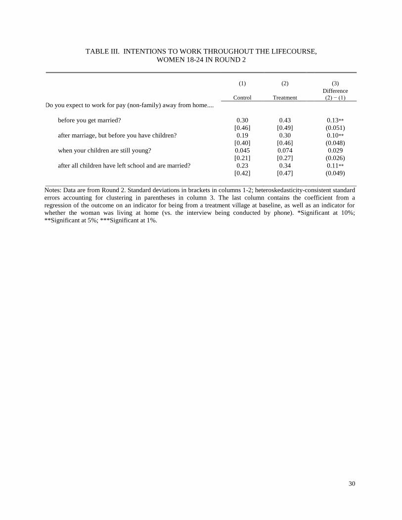
30

TABLE III. INTENTIONS TO WORK THROUGHOUT THE LIFECOURSE,

WOMEN 18-24 IN ROUND 2

(1) (2) (3)

Control

Treatment

Difference

(2) − (1)

Do you expect to work for pay (non-family) away from home....

before you get married? 0.30 0.43 0.13**

[0.46] [0.49] (0.051)

after marriage, but before you have children? 0.19 0.30 0.10**

[0.40] [0.46] (0.048)

when your children are still young? 0.045 0.074 0.029

[0.21] [0.27] (0.026)

after all children have left school and are married? 0.23 0.34 0.11**

[0.42] [0.47] (0.049)

Notes: Data are from Round 2. Standard deviations in brackets in columns 1-2; heteroskedasticity-consistent standard

errors accounting for clustering in parentheses in column 3. The last column contains the coefficient from a

regression of the outcome on an indicator for being from a treatment village at baseline, as well as an indicator for

whether the woman was living at home (vs. the interview being conducted by phone). *Significant at 10%;

**Significant at 5%; ***Significant at 1%.

31

TABLE IV. EFFECT OF THE INTERVENTION ON HUMAN CAPITAL

PANEL A. WOMEN

(1) (2) (3) (4)

Enrolled in Training

(18-24)

Enrolled in School

(6-17)

BMI-for-Age

(5-15)

Height-for-Age

(5-15)

Treatment 0.028*** 0.050*** 0.24*** 0.063 (0.008) (0.015) (0.070) (0.066)

R2 0.010 0.004 0.007 0.001

Observations 1,278 2,264 2,031 2,031

Control Group Mean 0.005 0.76 -1.25 -2.02

PANEL B. MEN

Enrolled in Training

(18-24)

Enrolled in School

(6-17)

BMI-for-Age

(5-15)

Height-for-Age

(5-15)

Treatment 0.003 0.010 -0.020 0.005 (0.004) (0.011) (0.076) (0.052)

R2 0.000 0.001 0.000 0.000

Observations 1,442 2,511 2,295 2,295

Control Group Mean 0.004 0.81 -1.29 -1.99

Notes: Heteroskedasticity-consistent standard errors accounting for clustering at the village-level in parentheses.

All dependent variables measured in Round 2; the number ranges in parentheses indicate the age range over which

the regression is estimated. The regressions contain only an indicator for coming from a treatment village, with no

additional covariates. BMI-for-Age and Height-for-Age are z-scores. ***Significant at 1 percent level.

32

TABLE V. EFFECT OF THE INTERVENTION ON MARRIAGE AND FERTILITY,

AGES 18-24 IN ROUND 2

PANEL A. WOMEN (1) (2) (3) Married Gave Birth Desired Fertility

Treatment -0.051** -0.057** -0.35*** (0.024) (0.026) (0.078)

R2 0.003 0.003 0.018

Observations 1,278 1,278 1,226

Control Group Mean 0.71 0.43 3.0

PANEL B. MEN

Married Gave Birth Desired Fertility

Treatment -0.002 -0.009 0.027 (0.025) (0.018) (0.066)

R2 0.000 0.000 0.000

Observations 1,442 1,442 1,437

Control Group Mean 0.44 0.15 3.3

Notes: Heteroskedasticity-consistent standard errors accounting for clustering at the village-

level in parentheses. All dependent variables measured in Round 2. The regressions contain

only an indicator for coming from a treatment village, with no additional covariates.

*Significant at 10 percent level. **Significant at 5 percent level. ***Significant at 1 percent

level.

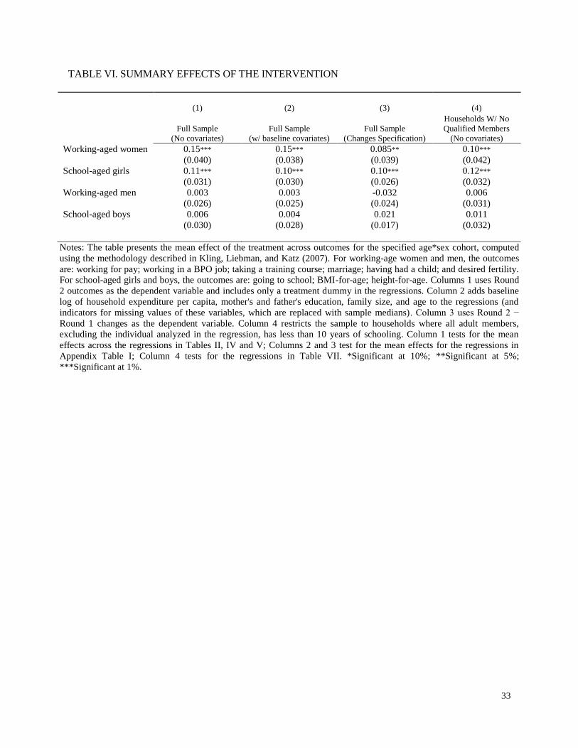
33

TABLE VI. SUMMARY EFFECTS OF THE INTERVENTION

(1) (2) (3) (4)

Full Sample

(No covariates)

Full Sample

(w/ baseline covariates)

Full Sample

(Changes Specification)

Households W/ No

Qualified Members

(No covariates)

Working-aged women 0.15*** 0.15*** 0.085** 0.10***

(0.040) (0.038) (0.039) (0.042)

School-aged girls 0.11*** 0.10*** 0.10*** 0.12***

(0.031) (0.030) (0.026) (0.032)

Working-aged men 0.003 0.003 -0.032 0.006

(0.026) (0.025) (0.024) (0.031)

School-aged boys 0.006 0.004 0.021 0.011

(0.030) (0.028) (0.017) (0.032)

Notes: The table presents the mean effect of the treatment across outcomes for the specified age*sex cohort, computed

using the methodology described in Kling, Liebman, and Katz (2007). For working-age women and men, the outcomes

are: working for pay; working in a BPO job; taking a training course; marriage; having had a child; and desired fertility.

For school-aged girls and boys, the outcomes are: going to school; BMI-for-age; height-for-age. Columns 1 uses Round

2 outcomes as the dependent variable and includes only a treatment dummy in the regressions. Column 2 adds baseline

log of household expenditure per capita, mother's and father's education, family size, and age to the regressions (and

indicators for missing values of these variables, which are replaced with sample medians). Column 3 uses Round 2 −

Round 1 changes as the dependent variable. Column 4 restricts the sample to households where all adult members,

excluding the individual analyzed in the regression, has less than 10 years of schooling. Column 1 tests for the mean

effects across the regressions in Tables II, IV and V; Columns 2 and 3 test for the mean effects for the regressions in

Appendix Table I; Column 4 tests for the regressions in Table VII. *Significant at 10%; **Significant at 5%;

***Significant at 1%.

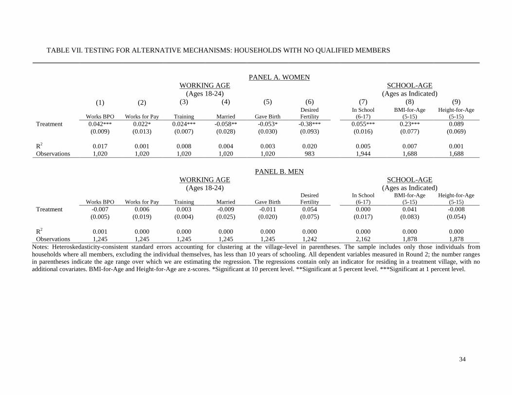
34

TABLE VII. TESTING FOR ALTERNATIVE MECHANISMS: HOUSEHOLDS WITH NO QUALIFIED MEMBERS

PANEL A. WOMEN

WORKING AGE

(Ages 18-24)

SCHOOL-AGE

(Ages as Indicated)

(1) (2) (3) (4) (5) (6) (7) (8) (9)

Works BPO Works for Pay Training Married

Gave Birth

Desired

Fertility

In School

(6-17)

BMI-for-Age

(5-15)

Height-for-Age

(5-15)

Treatment 0.042*** 0.022* 0.024*** -0.058** -0.053* -0.38*** 0.055*** 0.23*** 0.089

(0.009) (0.013) (0.007) (0.028) (0.030) (0.093) (0.016) (0.077) (0.069)

R2 0.017 0.001 0.008 0.004 0.003 0.020 0.005 0.007 0.001

Observations 1,020 1,020 1,020 1,020 1,020 983 1,944 1,688 1,688

PANEL B. MEN

WORKING AGE

(Ages 18-24)

SCHOOL-AGE

(Ages as Indicated)

Works BPO Works for Pay Training Married

Gave Birth

Desired

Fertility

In School

(6-17)

BMI-for-Age

(5-15)

Height-for-Age

(5-15)

Treatment -0.007 0.006 0.003 -0.009 -0.011 0.054 0.000 0.041 -0.008

(0.005) (0.019) (0.004) (0.025) (0.020) (0.075) (0.017) (0.083) (0.054)

R2 0.001 0.000 0.000 0.000 0.000 0.000 0.000 0.000 0.000

Observations 1,245 1,245 1,245 1,245 1,245 1,242 2,162 1,878 1,878

Notes: Heteroskedasticity-consistent standard errors accounting for clustering at the village-level in parentheses. The sample includes only those individuals from

households where all members, excluding the individual themselves, has less than 10 years of schooling. All dependent variables measured in Round 2; the number ranges

in parentheses indicate the age range over which we are estimating the regression. The regressions contain only an indicator for residing in a treatment village, with no

additional covariates. BMI-for-Age and Height-for-Age are z-scores. *Significant at 10 percent level. **Significant at 5 percent level. ***Significant at 1 percent level.

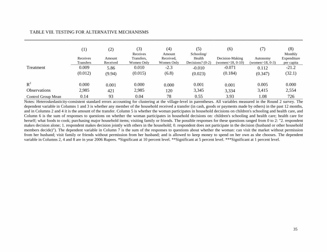
35

TABLE VIII. TESTING FOR ALTERNATIVE MECHANISMS

(1) (2) (3) (4) (5) (6) (7) (8)

Receives

Transfers

Amount

Received

Receives

Transfers,

Women Only

Amount

Received,

Women Only

Schooling/

Health

Decisions? (0-2)

Decision-Making

(women>18, 0-10)

Autonomy

(women>18, 0-3)

Monthly

Expenditure

per capita

Treatment 0.009 5.86 0.010 -2.3 -0.010 -0.071 0.112 -21.2

(0.012) (9.94) (0.015) (6.8) (0.023) (0.184) (0.347) (32.1)

R

2 0.000 0.001 0.000 0.000 0.001 0.001 0.005 0.000

Observations 2,985 421 2,985 120 3,345 3,334 3,415 2,554

Control Group Mean 0.14 93 0.04 78 0.55 3.93 1.08 726 Notes: Heteroskedasticity-consistent standard errors accounting for clustering at the village-level in parentheses. All variables measured in the Round 2 survey. The

dependent variable in Columns 1 and 3 is whether any member of the household received a transfer (in cash, goods or payments made by others) in the past 12 months,

and in Columns 2 and 4 it is the amount of the transfer. Column 5 is whether the woman participates in household decisions on children's schooling and health care, and

Column 6 is the sum of responses to questions on whether the woman participates in household decisions on: children's schooling and health care; health care for

herself; what foods to cook; purchasing major household items; visiting family or friends. The possible responses for these questions ranged from 0 to 2: "2. respondent

makes decision alone; 1. respondent makes decision jointly with others in the household; 0. respondent does not participate in the decision (husband or other household

members decide)"). The dependent variable in Column 7 is the sum of the responses to questions about whether the woman: can visit the market without permission

from her husband; visit family or friends without permission from her husband; and is allowed to keep money to spend on her own as she chooses. The dependent

variable in Columns 2, 4 and 8 are in year 2006 Rupees. *Significant at 10 percent level. **Significant at 5 percent level. ***Significant at 1 percent level.

36

APPENDIX FIGURE I. MAP OF THE SURVEY AREA

Uttar Pradesh Rajasthan

Punjab

Haryana Delhi

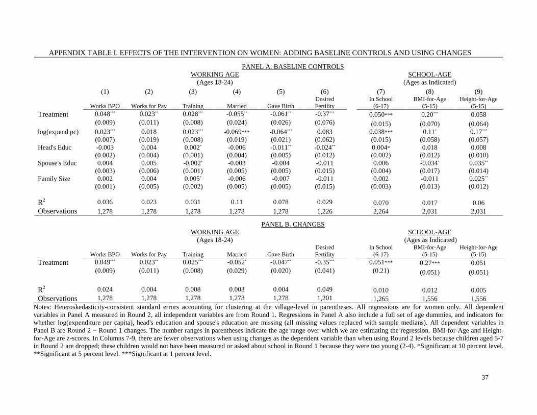
37

APPENDIX TABLE I. EFFECTS OF THE INTERVENTION ON WOMEN: ADDING BASELINE CONTROLS AND USING CHANGES

PANEL A. BASELINE CONTROLS

WORKING AGE

(Ages 18-24)

SCHOOL-AGE

(Ages as Indicated)

(1) (2) (3) (4) (5) (6) (7) (8) (9)

Works BPO Works for Pay Training Married

Gave Birth

Desired

Fertility

In School

(6-17)

BMI-for-Age

(5-15)

Height-for-Age

(5-15)

Treatment 0.048*** 0.023** 0.028*** -0.055** -0.061** -0.37*** 0.050*** 0.20*** 0.058

(0.009) (0.011) (0.008) (0.024) (0.026) (0.076) (0.015) (0.070) (0.064)

log(expend pc) 0.023*** 0.018 0.023*** -0.069*** -0.064*** 0.083 0.038*** 0.11* 0.17*** (0.007) (0.019) (0.008) (0.019) (0.021) (0.062) (0.015) (0.058) (0.057)

Head's Educ -0.003 0.004 0.002* -0.006 -0.011** -0.024** 0.004* 0.018 0.008 (0.002) (0.004) (0.001) (0.004) (0.005) (0.012) (0.002) (0.012) (0.010)

Spouse's Educ 0.004 0.005 -0.002* -0.003 -0.004 -0.011 0.006 -0.034* 0.035**

(0.003) (0.006) (0.001) (0.005) (0.005) (0.015) (0.004) (0.017) (0.014)

Family Size 0.002 0.004 0.005* -0.006 -0.007 -0.011 0.002 -0.011 0.025**

(0.001) (0.005) (0.002) (0.005) (0.005) (0.015) (0.003) (0.013) (0.012)

R2 0.036 0.023 0.031 0.11 0.078 0.029 0.070 0.017 0.06

Observations 1,278 1,278 1,278 1,278 1,278 1,226 2,264 2,031 2,031

PANEL B. CHANGES

WORKING AGE

(Ages 18-24)

SCHOOL-AGE

(Ages as Indicated)

Works BPO Works for Pay Training Married

Gave Birth

Desired

Fertility

In School

(6-17)

BMI-for-Age

(5-15)

Height-for-Age

(5-15)

Treatment 0.049*** 0.023** 0.025*** -0.052* -0.047** -0.35*** 0.051*** 0.27*** 0.051

(0.009) (0.011) (0.008) (0.029) (0.020) (0.041) (0.21) (0.051) (0.051)

R2 0.024 0.004 0.008 0.003 0.004 0.049 0.010 0.012 0.005

Observations 1,278 1,278 1,278 1,278 1,278 1,201 1,265 1,556 1,556

Notes: Heteroskedasticity-consistent standard errors accounting for clustering at the village-level in parentheses. All regressions are for women only. All dependent

variables in Panel A measured in Round 2, all independent variables are from Round 1. Regressions in Panel A also include a full set of age dummies, and indicators for

whether log(expenditure per capita), head's education and spouse's education are missing (all missing values replaced with sample medians). All dependent variables in

Panel B are Round 2 − Round 1 changes. The number ranges in parentheses indicate the age range over which we are estimating the regression. BMI-for-Age and Height-

for-Age are z-scores. In Columns 7-9, there are fewer observations when using changes as the dependent variable than when using Round 2 levels because children aged 5-7

in Round 2 are dropped; these children would not have been measured or asked about school in Round 1 because they were too young (2-4). *Significant at 10 percent level.

**Significant at 5 percent level. ***Significant at 1 percent level.

38

APPENDIX TABLE II. MEANS, STANDARD DEVIATIONS AND TESTS OF DIFFERENCES,

ATTRITING VS. NON-ATTRITING HOUSEHOLDS

(1) (2) (3)

Non-Attriters Attriters Diff. (2) − (1)

Log (expenditure per capita) 6.36 6.17 -0.19***

[0.66] [0.63] (0.063)

Head's years of schooling 3.79 3.37 -0.41

[3.77] [3.64] (0.33)

Spouse's years of schooling 1.80 1.70 -0.10

[2.67] [2.76] (0.27)

Family size 5.59 5.41 -0.17

[2.45] [2.14] (0.20)

Age (Female): 5-24 14.0 14.8 0.82

[5.60] [6.09] (0.50)

Age (Male): 5-24 14.0 13.2 -0.73

[5.50] [5.93] (0.52)

% women 15-21 married 0.35 0.43 0.077

[0.48] [0.50] (0.082)

% women 15-21 have given birth 0.27 0.36 0.089

[0.44] [0.48] (0.076)

% men 15-21 married 0.21 0.15 -0.061

[0.41] [0.36] (0.060)

% men 15-21 whose wife has had a child 0.047 0.049 0.002

[0.28] [0.35] (0.033)

% women 18 - 24 work for pay 0.20 0.12 -0.08

[0.40] [0.26] (0.052)

In school: girls 6-17 0.73 0.70 -0.030

[0.44] [0.46] (0.058)

In school: boys 6-17 0.80 0.85 0.054

[0.40] [0.35] (0.038)

BMI-for-age (z-score): girls 5-15 -1.25 -1.30 -0.047

[1.36] [1.32] (0.15)

BMI-for-age (z-score): boys 5-15 -1.30 -1.58 -0.28

[1.64] [1.43] (0.19)

Height-for-age (z-score): girls 5-15 -2.03 -2.04 -0.010

[1.35] [1.30] (0.16)

Height-for-age (z-score): boys 5-15 -2.02 -1.96 0.060

[1.38] [1.30] (0.17)

Notes: Values for variables collected in the Round 1 survey (September-October, 2003). Standard deviations

in brackets in columns 1-4; heteroskedasticity-consistent standard errors accounting for clustering in

parentheses in column 5. The last column contains t-tests of the difference in means between the control and

the treatment samples. *Significant at 10%; **Significant at 5%; ***Significant at 1%.

39

APPENDIX TABLE III. CORRELATES OF ATTRITION

(1) (2) (3) (4)

Entire Household

Women

18-24

Girls

6-17

Girls

5-15

Treatment 0.009 0.006 -0.001 0.003

(0.010) (0.013) (0.011) (0.013)

Log (expend. per capita) -0.016** -0.030** -0.009 -0.006

(0.007) (0.012) (0.009) (0.011)

Head's years of schooling -0.002 0.001 -0.0001 0.001

(0.001) (0.002) (0.002) (0.002)

Spouse's years of schooling 0.002 -0.001 -0.001 -0.003

(0.002) (0.003) (0.003) (0.003)

Family size 0.0005 0.004 0.003 -0.006**

(0.002) (0.002) (0.002) (0.002)

Has land -0.045*** -0.026* -0.013 -0.005

(0.009) (0.014) (0.013) (0.016)

Head's Age -0.003*** -0.001 0.000 0.000

(0.001) (0.001) (0.000) (0.001)

R2 0.010 0.020 0.004 0.006

Observations 3,199 1,361 2,391 2,130

Notes: Heteroskedasticity-consistent standard errors accounting for clustering at the village-level in parentheses. All

variables measured in the Round 2 survey. The dependent variable is an indicator for attrition. All regressions also

include a set of age dummies and indicators for whether log expenditure, and head's and spouse's years of schooling

are missing (missing values are replaced with medians). *Significant at 10 percent level. **Significant at 5 percent

level. ***Significant at 1 percent level.

40

APPENDIX TABLE IV. TREATMENT EFFECTS REWEIGHTED BY INVERSE PROBABILITY OF ATTRITION

PANEL A. WOMEN

WORKING AGE

(Ages 18-24)

SCHOOL-AGE

(Ages as Indicated)

(1) (2) (3) (4) (5) (6) (7) (8) (9)

Works BPO Works for Pay Training Married

Gave Birth

Desired

Fertility

In School

(6-17)

BMI-for-Age

(5-15)

Height-for-Age

(5-15)

Treatment 0.045*** 0.022* 0.022*** -0.056** -0.059** -0.33*** 0.051*** 0.19*** 0.057

(0.010) (0.011) (0.007) (0.025) (0.028) (0.084) (0.015) (0.071) (0.068)

R2 0.024 0.024 0.008 0.004 0.004 0.016 0.004 0.005 0.001

Observations 1,278 1,278 1,278 1,278 1,278 1,226 2,264 2,031 2,031

PANEL B. MEN

WORKING AGE

(Ages 18-24)

SCHOOL-AGE

(Ages as Indicated)

Works BPO Works for Pay Training Married

Gave Birth

Desired

Fertility

In School

(6-17)

BMI-for-Age

(5-15)

Height-for-Age

(5-15)

Treatment -0.005 0.002 0.005 0.007 -0.014 0.017 0.011 0.058 0.006

(0.005) (0.012) (0.004) (0.025) (0.018) (0.070) (0.016) (0.079) (0.057)

R2 0.001 0.001 0.001 0.000 0.001 0.000 0.000 0.000 0.000

Observations 1,442 1,442 1,442 1,442 1,442 1,437 2,511 2,295 2,295

Notes: Heteroskedasticity-consistent standard errors accounting for clustering at the village-level in parentheses. Estimates from OLS regressions using the inverse

probability of attrition (estimated from separate probit models, as in Appendix Table IV) as sample weights. All dependent variables measured in Round 2; the number

ranges in parentheses indicate the age range over which we are estimating the regression. The regressions contain only an indicator for residing in a treatment village, with

no additional covariates. BMI-for-Age and Height-for-Age are z-scores. *Significant at 10 percent level. **Significant at 5 percent level. ***Significant at 1 percent level.

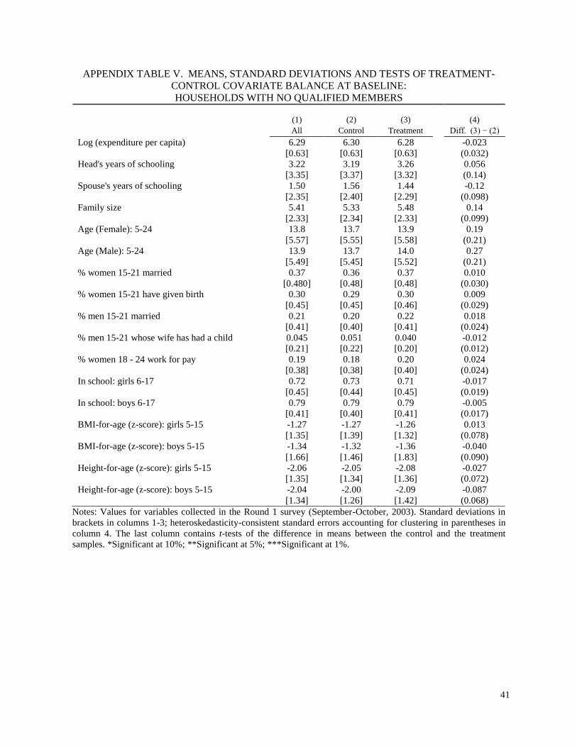
41

APPENDIX TABLE V. MEANS, STANDARD DEVIATIONS AND TESTS OF TREATMENT-

CONTROL COVARIATE BALANCE AT BASELINE:

HOUSEHOLDS WITH NO QUALIFIED MEMBERS

(1) (2) (3) (4)

All Control Treatment Diff. (3) − (2)

Log (expenditure per capita) 6.29 6.30 6.28 -0.023

[0.63] [0.63] [0.63] (0.032)

Head's years of schooling 3.22 3.19 3.26 0.056

[3.35] [3.37] [3.32] (0.14)

Spouse's years of schooling 1.50 1.56 1.44 -0.12

[2.35] [2.40] [2.29] (0.098)

Family size 5.41 5.33 5.48 0.14

[2.33] [2.34] [2.33] (0.099)

Age (Female): 5-24 13.8 13.7 13.9 0.19

[5.57] [5.55] [5.58] (0.21)

Age (Male): 5-24 13.9 13.7 14.0 0.27

[5.49] [5.45] [5.52] (0.21)

% women 15-21 married 0.37 0.36 0.37 0.010

[0.480] [0.48] [0.48] (0.030)

% women 15-21 have given birth 0.30 0.29 0.30 0.009

[0.45] [0.45] [0.46] (0.029)

% men 15-21 married 0.21 0.20 0.22 0.018

[0.41] [0.40] [0.41] (0.024)

% men 15-21 whose wife has had a child 0.045 0.051 0.040 -0.012

[0.21] [0.22] [0.20] (0.012)

% women 18 - 24 work for pay 0.19 0.18 0.20 0.024

[0.38] [0.38] [0.40] (0.024)

In school: girls 6-17 0.72 0.73 0.71 -0.017

[0.45] [0.44] [0.45] (0.019)

In school: boys 6-17 0.79 0.79 0.79 -0.005

[0.41] [0.40] [0.41] (0.017)

BMI-for-age (z-score): girls 5-15 -1.27 -1.27 -1.26 0.013

[1.35] [1.39] [1.32] (0.078)

BMI-for-age (z-score): boys 5-15 -1.34 -1.32 -1.36 -0.040

[1.66] [1.46] [1.83] (0.090)

Height-for-age (z-score): girls 5-15 -2.06 -2.05 -2.08 -0.027

[1.35] [1.34] [1.36] (0.072)

Height-for-age (z-score): boys 5-15 -2.04 -2.00 -2.09 -0.087

[1.34] [1.26] [1.42] (0.068)

Notes: Values for variables collected in the Round 1 survey (September-October, 2003). Standard deviations in

brackets in columns 1-3; heteroskedasticity-consistent standard errors accounting for clustering in parentheses in

column 4. The last column contains t-tests of the difference in means between the control and the treatment

samples. *Significant at 10%; **Significant at 5%; ***Significant at 1%.