individual channel analysis of the thyristor-controlled - diva portal

Volume 11, Issue 2 2010 Article 4

International Journal of EmergingElectric Power Systems

Individual Channel Analysis of the Thyristor-Controlled Series Compensator Performance

Carlos Ernesto Ugalde Loo, University of GlasgowEnrique Acha, University of Glasgow

Eduardo Liceaga-Castro, Universidad Carlos III de MadridLuigi Vanfretti, Rensselaer Polytechnic Institute

Recommended Citation:Ugalde Loo, Carlos Ernesto; Acha, Enrique; Liceaga-Castro, Eduardo; and Vanfretti, Luigi(2010) "Individual Channel Analysis of the Thyristor-Controlled Series CompensatorPerformance," International Journal of Emerging Electric Power Systems: Vol. 11: Iss. 2,Article 4.DOI: 10.2202/1553-779X.2190

Brought to you by | Kungliga Tekniska Hogskola (Kungliga Tekniska Hogskola)Authenticated | 172.16.1.226

Download Date | 1/23/12 4:24 PM

Individual Channel Analysis of the Thyristor-Controlled Series Compensator PerformanceCarlos Ernesto Ugalde Loo, Enrique Acha, Eduardo Liceaga-Castro, and Luigi

Vanfretti

Abstract

The TCSC is the electronically-controlled counterpart of the conventional series bank ofcapacitors. A mature member of the FACTS technology, the TCSC has the ability to regulatepower flows along the compensated line and to rapidly modulate its effective impedance. In thispaper its performance is evaluated using Individual Channel Analysis and Design. Fundamentalanalysis is carried out to explain the generator dynamic behavior as affected by the TCSC.Moreover, a control system design for the system is presented, with particular emphasis in theclosed-loop performance and stability and structural robustness assessment. It is formally shownthat the incorporation of a TCSC operating in its capacitive range improves the dynamicalperformance of the synchronous machine by decreasing the electrical distance and thereforeconsiderably reducing the awkward switchback characteristic exhibited by synchronousgenerators. It is also formally proven in the paper that the inductive operation should be avoided asit impairs system operation. In general, the TCSC inclusion brings on fragility into the globalsystem, making it non-minimum phase and introducing adverse dynamics in the speed channel ofthe synchronous machine. Moreover, it is shown that the minimum-phase condition may also bepresent in cases featuring high capacitive compensation levels.

KEYWORDS: TCSC, synchronous generator, ICAD, stability, robustness

Author Notes: This work was supported by CONACyT, México.



Introduction

Active power transfers between areas may be substantially increased and adjusted very effectively by varying the net series impedance of the series compensated line. The Thyristor-Controlled Series Compensator (TCSC), an already installed and mature member of the second generation of FACTS devices, is the electronically-controlled counterpart of the conventional series bank of capacitors (IEEE/CIGRE, 1995). Its major benefits are its ability to regulate power flows along the compensated line and to rapidly modulate the effective impedance of the line in response to dynamic events in the vicinity of the line – allowing a smooth control of transmission line compensation levels.

Experience with the operation of series compensation facilities has encouraged power system planners to look at the TCSC as a realistic solution for providing better control in the high-voltage side of the power network (see, for instance, the work Jancke, et al., 1975, Iliceto and Cinieri, 1977, and Angquist, et al., 1993). This fact provides the motivation to carry out fundamental studies of the dynamic behavior of TCSC-upgraded transmission systems. So far, valuable transfer function block-diagram models of the synchronous machine – TCSC system have been developed by Aree (2000). Such a representation yields physical insight and understanding of the system behavior. However, although it enables a transparent analysis of the interaction between internal variables in terms of constants and transfer functions that fully encapsulate all key dynamic parameters, not all interactions between the various variables may be useful for control system design purposes.

A successful integration of FACTS devices into power systems networks is of great importance for all sectors of the market: power generation, transmission, distribution, and high-voltage power electronics equipment manufacturers. The proper understanding of the TCSC will positively contribute to this task. Nevertheless, further research is required as the existing analysis tools, although applicable to large-scale systems (Kundur, et al., 1990), may lack physical transparency. As previously discussed by Leithead and O’Reilly (1992) and Ugalde, et al. (2007), Individual Channel Analysis and Design (ICAD) provides an alternative and very insightful control-oriented framework with which to carry out small-signal stability assessments.

Building into this positive experience, preliminary work on the performance of a synchronous generator – TCSC system connected to an infinite bus via a tie-line reactance using the ICAD framework was reported by Ugalde, et al. (2008b). In that paper, fundamental analysis is carried out to explain the generator dynamic behavior as affected by the TCSC. The analysis and synthesis of a control design is carried out and an assessment of its robustness and performance is presented.

1

Ugalde Loo et al.: Individual Channel Analysis of the TCSC Performance



In this paper the emphasis is on the closed-loop performance and stability and structural robustness assessment of the synchronous generator – TCSC – infinite bus system, including extreme operating conditions. Study cases include the effect of series compensation in weak and strong transmission systems, maximum capacitive compensation, and the little studied inductive region of operation. The system performance with TCSC and with no TCSC is compared and conclusions are drawn.

It should be remarked that the synchronous generator – TCSC – infinite bus system selected for study in this paper offers the best opportunity available for gaining a fundamental understanding of the complex dynamic interactions that take place between the synchronous generator and the TCSC, with the infinite bus screening this set from possible unwelcoming external influences in the form of other machines’ dynamic signals. Furthermore, the synchronous generator – TCSC – infinite bus system has also a very practical connotation in the area of power systems series compensation. Series compensation applies to long-distance transmission systems, those in excess of 300 km and up to 700 km, where long-distance HVDC begins to be economically competitive; even though the example of El Chocón in Argentina, which is a 1000 km long transmission line, uses two sets of series capacitors symmetrically placed at 1/3 and 2/3 along the line. Another example is the 500 km long transmission corridor in South East Mexico responsible for transporting the bulk of the Mexican hydro-power resource to Central Mexico. The transmission corridor is series compensated at an intermediate switching substation. A similar situation arises in Sweden where the hydro-power generated in Northern Sweden is transported to the South over a very considerable distance. Apart from Sweden where a TCSC has been installed, the other two examples use fix series capacitive compensation. Perhaps more importantly is the fact that series compensation applies to portions of the power system that resemble very much a synchronous generator – TCSC – infinite bus system, with the infinite bus being a strong point of the network, which invariably is a point of a highly meshed network, as it would be case in Southern Sweden and Central Mexico. Although power systems do contain a large number of synchronous machines, in many countries, large portions of the power system are not particularly highly meshed. Electro-mechanically or electronically-controlled series compensation finds application in AC long-distance transmission that resembles very much the layout of the test system selected for the study, namely synchronous generator – TCSC – infinite bus system.

2

International Journal of Emerging Electric Power Systems, Vol. 11 [2010], Iss. 2, Art. 4

DOI: 10.2202/1553-779X.2190



1. System under study

The synchronous machine dynamic representation used to derive the model presented here is based on the work of Hammons and Winning (1971). The system under study is shown in figure 1.

Figure 1. Synchronous generator – TCSC system

The test system of figure 1 is used to assess the influence that the TCSC exerts on the generator dynamic characteristic. It consists of one synchronous generator feeding into an infinite-bus system via a TCSC compensated tie-line. A synchronous machine of 6 p.u. on a base power of 100 MVA is considered, with parameters given by Saidy and Hughes (1994) and included for completeness in Appendix 3.

Remark: A practical system will undoubtedly have several machines, but it will not necessarily be highly meshed in all its parts. On the other hand, series compensation applies to long-distance transmission systems – which are radial systems.

1.1. Block diagram representation

The small-signal model is developed from first principles, by using the non-linear and algebraic equations that represent the synchronous generator – TCSC system. In order to study the dynamic interaction between the generator and the TCSC, the effects of the field and damping windings in the d and q-axis should be included. Therefore, a 5th order salient-pole synchronous generator model is considered, which accounts for the effects of the generator main field winding plus one damper winding in the d-axis and one in the q-axis. A straightforward but cumbersome linearization exercise of the dynamic equations produces the following expressions in the s-domain (Aree, 2000):

( ) ( ) ( ) ( ) ( )'' ''1 2 2 1e q d d TCSCP s K s K E s K E s K sδ αΔ = Δ + Δ − Δ + Δ (1)

( ) ( ) ( ) ( ) ( )'' ''5 6 6 3t q d d TCSCe s K s K E s K E s K sδ αΔ = Δ + Δ + Δ + Δ (2)

3




( ) ( ) ( ) ( ) ( )'' ''5 6 6 3TCSC n n q dn d TCSC nI s K s K E s K E s K sδ αΔ = Δ + Δ − Δ + Δ (3)

( ) ( ) ( ) ( ) ( ) ( ) ( )''3 4 2q fd TCSCE s K s E s K s s K s sδ αΔ = Δ − Δ − Δ (4)

( ) ( ) ( ) ( )''4 2d d TCSC dE K s s K s sδ αΔ = Δ + Δ (5)

( ) ( ) ( ) ( )12 m es P s P s D s

Hsω ω⎡ ⎤Δ = ⋅ Δ − Δ − Δ⎣ ⎦ (6)

( ) ( )0s ss

ωδ ωΔ = Δ (7)

where the coefficients and transfer functions of equations (1)–(7) are given in Appendix 1. The previous equations are used to form the block diagram representation for the model, shown in figure 2. There are three feedback subsystems in the generator – TCSC block diagram, i.e., excitation, turbine-governor and TCSC impedance control loops. This is in addition to the 3-input 3-output generator TCSC – system, whose outputs of interest are generator speed (Δω), generator output voltage (Δet) and TCSC current (ΔITCSC) flowing through the tie-line.

Figure 2. Detailed block diagram for a synchronous generator – TCSC system

4


DOI: 10.2202/1553-779X.2190



The main function of the impedance control loop of the TCSC is to schedule an amount of electrical power to be delivered through the tie-line. The feedback control signal is directly taken from the current (ΔITCSC) flowing through the TCSC component. Hence, ΔITCSC brings a change from the generator’s flux linkages in the d and q-axis and rotor angle via coefficients K6n, K6dn and K5n, which is compared with the reference ΔITCSC,ref in order to adjust the firing angle at the desired power flows level.

Similarly to the case of the SVC (see, for instance, the work of Aree and Acha, 1999, Aree, 2000, and Ugalde, et al., 2008a), an incremental change in the electrical power of the generator is employed here to investigate the dynamic interactions between the generator and the TCSC. Moreover, the TCSC branches influencing the generator’s behaviour are similar to those of the SVC, as evidenced by the block diagram presented in the work of Aree and Acha (1999). An incremental change in the TCSC firing angle leads to a direct change in the output power of the generator, which is made up of three individual electrical power loops, namely ΔPTCSC, ΔPed, and ΔPeq. ΔPTCSC is the component of the generator’s output power that is directly channelled through coefficient KTCSC1

and it is due to a change in TCSC impedance (ΔXTCSC). ΔPed and ΔPeq are portions of the output power produced by the d and q-axis flux linkages, respectively. The TCSC may influence the power produced by the flux linkages through coefficient KTCSC3 and the transfer functions KTCSC2(s) and KTCSC2d(s). Once the firing angle is changed to increase the TCSC contribution (in the capacitive mode of operation), all coefficients and transfer functions making up the entire system will be affected due to a reduction of the tie-line’s impedance.

The block diagram of the generator – TCSC system yields unique physical insight as to how the TCSC dynamically affects the generator. It enables a transparent analysis of the interaction between internal machine variables and the TCSC in terms of constants and transfer functions that encapsulate fully all key dynamic parameters of the system. However, caution needs to be exercised since not all interactions between the various variables may be useful for control system design purposes. Such ambiguities can be avoided by working with the alternative control-oriented framework termed ICAD, a powerful analysis and design tool which is well suited to the task of carrying out small signal stability assessments. The dynamical behaviour and structure of the system can be described in a global context in which the characteristics of the individual transfer functions are not essential.

5




1.2. TCSC characteristic

The TCSC is connected in series with the tie-line, as shown in figure 3. The active power flow leaving node n can be adjusted by controlling the TCSC impedance (XTCSC). This is achieved by suitably changing the thyristor’s firing angle.

Figure 3. Configuration of the TCSC connected in series with a tie-line

The expression for the fundamental frequency of the TCSC impedance, as a function of the thyristor’s firing angle, is given as (Helbing and Karady, 1994):

( ) ( ){ }( ) ( ) ( ){ }

1

22

2 sin 2

cos tan tan

TCSC CX X C

C

π α π α

π α λ λ π α π α

⎡ ⎤= − + − + − +⎣ ⎦

⎡ ⎤− − − − −⎣ ⎦ (8)

For a small variation, the derivative value of the TCSC impedance characteristic, F(α) = ∂XTCSC/∂α, is given by

( ) ( ) ( )( )

( ) ( ){ }

2 2

1 2 2

2

cos2 1 cos 2 1

cos

sin 2 tan tan

F C C

C

λ π αα α

λ π α

α λ λ π α π α

⎧ ⎫−⎪ ⎪= − + + −⎨ ⎬⎡ ⎤−⎪ ⎪⎣ ⎦⎩ ⎭

⎡ ⎤+ − − −⎣ ⎦

(9)

where

1C LCX XC

π+

= 2

24 LC

L

XCXπ

= 0 C

L

XX

ωλ

ω= =

C L

LCC L

X XXX X

=−

2 20

1 C

L

XLC

ωX

ω= =

6


DOI: 10.2202/1553-779X.2190



Consider a TCSC with inductive and capacitive reactance values corresponding to those of the fully operational Kayenta TCSC installation (reported by Christl, et al., 1992, and included in Appendix 3). Figure 4 shows the fundamental frequency reactance as a function of α and its derivative F(α).

From figure 4 it can be observed that the impedance characteristic has two distinctive regions of operation, one inductive and one capacitive. The capacitive region lays to the right of a firing angle of approximately 142.6°. For firing angle values near the resonant point the variations of XTCSC are quite large even for a small variation in the controlling firing angle. If an increase of TCSC impedance in the capacitive mode is required then the firing angle value should move towards the resonant point. Also, F(α) has always positive values in the TCSC firing angle range. The effect of F(α) appears in many of the system coefficients of the block-diagram model, as seen in Appendix 1.

Figure 4. TCSC impedance characteristic XTCSC and its derivative F(α) = ∂XTCSC/∂α for given parameters

The usual practice is to operate the TCSC in its capacitive region, aiming at decreasing the electrical length of the transmission line in order to increase active power flows. In this paper, extreme cases of series compensation will also be addressed. The maximum amount of series compensation for the system under study will be carefully examined. For completeness, operation in the inductive region of the TCSC will also be assessed.

7




1.3. Transfer matrix representation

The transfer matrix representation of the system is not only desirable but essential for the analysis of the synchronous generator – TCSC plant dynamics under the ICAD framework. After some arduous algebra, the following representation is arrived at,

( )( )

( )

( ) ( ) ( )( ) ( ) ( )( ) ( ) ( )

( )( )

( )

11 12 13

21 22 23

31 32 33

m

t fd

TCSC

s g s g s g s P se s g s g s g s E s

I s g s g s g s s

ω

α

⎡ ⎤ ⎡ ⎤ ⎡ ⎤Δ Δ⎢ ⎥ ⎢ ⎥ ⎢ ⎥Δ = Δ⎢ ⎥ ⎢ ⎥ ⎢ ⎥⎢ ⎥ ⎢ ⎥ ⎢ ⎥Δ Δ⎣ ⎦ ⎣ ⎦ ⎣ ⎦

(10)

or in a more compact form

( ) ( ) ( )s s s=y G u (11)

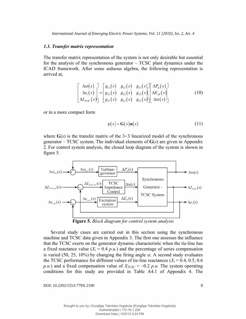
where G(s) is the transfer matrix of the 3×3 linearized model of the synchronous generator – TCSC system. The individual elements of G(s) are given in Appendix 2. For control system analysis, the closed loop diagram of the system is shown in figure 5.

Figure 5. Block diagram for control system analysis

Several study cases are carried out in this section using the synchronous machine and TCSC data given in Appendix 3. The first one assesses the influence that the TCSC exerts on the generator dynamic characteristic when the tie-line has a fixed reactance value (Xt = 0.4 p.u.) and the percentage of series compensation is varied (50, 25, 10%) by changing the firing angle α. A second study evaluates the TCSC performance for different values of tie-line reactances (Xt = 0.4, 0.5, 0.6p.u.) and a fixed compensation value of XTCSC = –0.2 p.u. The system operating conditions for this study are provided in Table A4.1 of Appendix 4. The

8


DOI: 10.2202/1553-779X.2190



numerical calculations show that for all these operating conditions all the individual elements gij(s) in (10) are stable and minimum-phase.

2. Multivariable analysis

In the framework afforded by ICAD, the dynamical structure of plant (10) is determined by input-output channels resulting from pairing each input to each output by means of diagonal controllers. For the case of the synchronous generator – TCSC system, the traditional pairing of inputs to outputs is given as (Aree, 2000):

( )( )

( )( )

( ) ( ) ( )( ) ( ) ( )

( ) ( ) ( )

1 1

2 2

3 3

0 0 :0 0 :0 0 :

m

fd t

TCSC

k s C s P s ss k s C s E s e s

k s C s s I s

ω

α

⎡ ⎤ ⎧ Δ → Δ⎪⎢ ⎥= ⇒ Δ → Δ⎨⎢ ⎥⎪⎢ ⎥ Δ → Δ⎣ ⎦ ⎩

K (12)

The diagonal controller given in (12), which considers pairings as ΔPm(s) Δω(s), ΔEfd(s) Δet(s) and Δα(s) ΔITCSC(s), agrees with that used for conventional controllers and this would be the only case considered in this paper. Coupling between channels is determined by Multivariable Structure Functions (MSF) Γi(s) as defined in the work of Leithead and O’Reilly (1992). These functions are indicators of the potential performance of feedback control. A small magnitude of MSF is amenable to a low signal interaction between channels.

The multivariable structure functions Γi(s), i = 1,2 (Γ3 = 0), are defined as

( ) ( ) ( )12... 1 12... 1/i i ii i iis g− −Γ = − G G (13)

where 1 2 ... ri i iG is the transfer function matrix obtained from the plant matrix G(s) by eliminating rows and columns of elements i1, i2, …, ir; and matrix 1 2 ... ri i i

jG is the transfer function matrix obtained from G(s) by setting diagonal element gjj of G(s) to zero before eliminating the rows and columns as in the definition of 1 2 ... ri i iG .

It should be noted that all MSFs associated to the model share some important common characteristics for both studies. Numerical calculation shows that they are stable and minimum-phase. Moreover, their Nyquist plots (not included) start to the left of the point (1,0). Such features ease the design process. After suitable analysis of the MSFs associated to the 3×3 system, the following remarks can be made about the channels: • The Multiple Channel M23(s) is highly coupled with the Individual Channel

C1(s) – the increase of series compensation decreases this coupling. Individual

9




Channels C2(s) and C3(s) within Multiple Channel M23(s) are lightly coupled – the increase of series compensation increases this coupling.

• M13(s) is lowly coupled with C2(s) – the increase of series compensation increases this coupling. C1(s) and C3(s) within M13(s) are highly coupled – the increase of series compensation decreases this coupling.

• M12(s) is highly coupled with C3(s) – the increase of series compensation decreases this coupling. C1(s) and C2(s) within M12(s) are lowly coupled – the increase of series compensation decreases this coupling.

(a)

(b) Figure 6. Assessments of Γ2_3(s) (Study 1): (a) Nyquist plot; (b) Bode plot

10


DOI: 10.2202/1553-779X.2190



(a)

(b) Figure 7. Assessments of Γ2_3(s) (Study 2): (a) Nyquist plot; (b) Bode plot

It can be safely stated that the TCSC together with the synchronous machine produces a highly coupled multivariable system regardless of the amount of series compensation and tie-line reactance value – particularly at low frequencies over the range of interest of 1–10 rad/s. It should be noted that the TCSC impedance control loop, represented by C3(s), tends to significantly couple with the speed channel of the synchronous generator, i.e., C1(s).

Within the ICAD context, Multiple Channel M12(s) represents the actual dynamics of the synchronous generator under the influence of the TCSC. Within Multiple Channel M12(s), MSF Γ2_3(s) gives a measure of coupling between Individual Channels C1(s) and C2(s) (speed and terminal voltage, respectively) of the synchronous generator. The Nyquist and Bode plots of MSF Γ2_3(s) for the operating conditions given in Tables A4.1 and A4.2 of Appendix 4 are shown in figures 6 and 7. These plots confirm that Individual Channels C1(s) and C2(s) are

11




lowly coupled and that an increase of series compensation decreases even more such coupling. In general, an increase in the tie-line reactance value, i.e., a series compensation reduction, will increase coupling.

The foregoing analysis is of paramount importance since it may lead to a control design strategy, which incidentally coincides with that put forward for the SVC by Ugalde, et al. (2008a). Since coupling in Multiple Channel M12(s) is low, it can be designed independently from Individual Channel C3(s). Consider the transfer matrix

( )( )( )

( ) ( ) ( )( ) ( ) ( )( ) ( ) ( )

( )( )( )

33 31 32

13 11 12

23 21 22

TCSC

m

t fd

I s g s g s g s ss g s g s g s P s

e s g s g s g s E s

αω

⎡ ⎤⎡ ⎤ ⎡ ⎤Δ Δ⎢ ⎥⎢ ⎥ ⎢ ⎥Δ = Δ⎢ ⎥⎢ ⎥ ⎢ ⎥⎢ ⎥⎢ ⎥ ⎢ ⎥Δ Δ⎣ ⎦ ⎣ ⎦ ⎣ ⎦

(14)

where the following partitioned system is used for the control design:

( ) ( ) ( )( ) ( ) ( ) ( )

( )11 12 1

21 22 2

s s s

s ss s s

⎡ ⎤ ⎡ ⎤= =⎢ ⎥ ⎢ ⎥

⎣ ⎦ ⎣ ⎦

G G K 0G K

G G 0 K (15)

( ) ( )( ) ( ) ( )

( )1 1

2 2

s s

s ss s

⎡ ⎤ ⎡ ⎤= =⎢ ⎥ ⎢ ⎥

⎣ ⎦ ⎣ ⎦

r yr y

r y (16)

with

( ) ( ) ( ) ( ) ( )11 33 12 31 32 s g s s g s g s⎡ ⎤= = ⎣ ⎦G G

( ) ( )( ) ( ) ( ) ( )

( ) ( )13 11 12

21 2223 21 22

g s g s g s

s sg s g s g s

⎡ ⎤ ⎡ ⎤= =⎢ ⎥ ⎢ ⎥

⎣ ⎦ ⎣ ⎦G G

( ) ( ) ( ) ( )( )

( ) ( ) ( ) ( )( )

11 3 2

2

11 3 2

2

r ss r s s

r s

y ss y s s

y s

⎡ ⎤= = ⎢ ⎥

⎣ ⎦

⎡ ⎤= = ⎢ ⎥

⎣ ⎦

r r

y y

( ) ( ) ( ) ( )( )

11 3 2

2

0

0k s

s k s sk s

⎡ ⎤= = ⎢ ⎥

⎣ ⎦K K

12


DOI: 10.2202/1553-779X.2190



The Individual Channel C3(s) is expressed by

( ) ( ) ( )( ) ( ) ( ) ( ) ( ) ( )( )

-1 -11 3 12 22 2 21 11 11 1

-1 13 33 12 22 2 21 331

s C s

k g s s s s s g s−

= = −

= −

M I G G H G G G K

G G H G (17)

where the multiple subsystem transfer function matrix H2(s) is given by

( ) ( ) ( ) ( ) ( )( ) 12 22 2 22 2s s s s s

−= +H G K I G K (18)

and subjected to the cross-reference disturbance

( ) ( ) ( ) ( )11 12 22 2s s s s−=D G G H (19)

Similarly, the Multiple Channel M12(s) is expressed by

( ) ( ) ( )( ) ( ) ( ) ( ) ( )( )

-1 -12 12 2x2 21 11 1 12 22 22 2

-1 -12x2 33 1 21 12 22 22 2

s s

g s h s s s s

= = −

= −

M M I G G H G G G K

I G G G G K (20)

where H1(s) is given by

( ) ( ) ( ) ( ) ( ) ( )( ) 11 1 3 33 3 331s h s k s g s k s g s

−= = +H (21)

and subjected to the cross-reference disturbance

( ) ( ) ( ) ( )12 33 1 21s g s h s s−=D G (22)

Assuming h1(s) = 1, the Multiple Channel M12(s) is designed as a separate 2x2 system. Once controllers k1(s) and k2(s) are obtained, H2 can be defined (that is, the interaction of M12(s) with C3(s)) and a controller k3(s) for the Individual Channel C3(s), as indicated in equation (17), can also be designed. After that, an expression for h1(s) (interaction with M12(s)) is calculated and controllers k1(s) and k2(s) are re-designed. The process is repeated until a suitable controller is achieved for all channels, with robustness assured for each individual channel, subsystems Hi(s), and MSFs γi(s).

Note: For more information on ICAD for m×m systems, the reader is referred to Appendix 5. For the system under study, notice that each Individual Channel can be written as in (A.1). Moreover, the evaluation of (A.1) with i = 3 provides

13




an expression equivalent to (17). C1 and C2 within the Multiple Channel M12 are defined likewise.

The control system design problem for a weak system is faced in very much the same way as for a strong system. However, the following inherent constraint should be kept in mind: the unavoidable decrease of system bandwidth to overcome the switch-back characteristic.

3. Control system design example

3.1. Study 1. Effect of series compensation variation in a weak tie-line

An assessment of the MSFs and transfer matrix associated to the operating conditions given in Table A4.1 of Appendix 4 yields the following diagonal controller

( )( )

( )( )

( )( )

( ) ( )( )( )

1

2

3

2

2

0 00 00 0

5.75 6.1 165.5 14 0.43 0.2diag , ,

5 7 0.7TCSC

k ss k s

k s

s s s k ss s s s s s

⎡ ⎤⎢ ⎥= ⎢ ⎥⎢ ⎥⎣ ⎦

⎡ ⎤+ + + +⎢ ⎥=

+ + +⎢ ⎥⎣ ⎦

1K

(23)

where kTCSC is a scalar gain for the TCSC impedance control loop which varies according to the level of compensation; for instance, kTCSC = –1 for 50%, –2 for 25% and –16 for 10% of compensation. As indicated in Table A4.1, the tie-line reactance is kept at a constant value of Xt = 0.4 p.u. The control system performance and stability robustness indicators are presented in figures 8–11.

From figures 8–11, it can be seen that the control system performance is adequate for all operating conditions, since controller (23) successfully decouples the generator channels for typical frequencies (given in the work of Kundur, 1994) and the speed regulation is effective for the lower frequency signals, blinding interactions with the higher frequency terminal voltage and the TCSC impedance control channels. However, it should be remarked that the performance tends to improve with the amount of series compensation provided by the TCSC. Furthermore, stability and structural robustness measures are higher with an increase of compensation. Notice that gains kTCSC of the impedance control loop in (23) are chosen in such a way that the bandwidths of the individual channels are maintained regardless of the amount of compensation while still providing adequate robustness margins, i.e., gain and phase margins over 6 dB and 40 deg, respectively (Kundur, 1994).

14


DOI: 10.2202/1553-779X.2190



(a)

(b)

(c) Figure 8. System performance (Study 1). Step response of: (a) Channel 1 (Tc1(s));

(b) Channel 2 (Tc2(s)); (c) Channel 3 (Tc3(s))

15




(a)

(b)

(c) Figure 9. System performance and stability robustness assessment (Study 1). Bode diagrams: (a) Channel 1 (C1(s)); (b) Channel 2 (C2(s)); (c) Channel 3

(C3(s))

16


DOI: 10.2202/1553-779X.2190



(a)

(b)

(c) Figure 10. Stability robustness assessment (Study 1). Bode diagrams:

(a) k1g11(s); (b) k2g22(s); (c) k3g33(s)

17




(a)

(b)

(c) Figure 11. Structural robustness assessment (Study 1). Nyquist diagrams:

(a) γ1(s); (b) γ2(s); (c) γ3(s)

18


DOI: 10.2202/1553-779X.2190



Remarks: Although the performance seems adequate, it is of paramount importance to realize that channel C3(s) is non-minimum phase. In fact, it can be seen from figure 11 that γ3(s) circles the point (1,0) twice in a clockwise direction for all operating conditions. Such a situation poses a major inconvenience for control system design and limits the system performance. It has to be kept in mind that even under disturbances, the bandwidth of C3(s) should be kept low, below the values of the unstable zero pair; otherwise, instability might arise. It should be remarked that the diagonal controller (23), by including an integral action in each of its individual elements, guarantees high gains at low frequencies and zero steady-state error. The extra lead zero-pole pair in k3(s) increases stability margins.

3.2. Study 2. Effect of fixed compensation on electrical distance

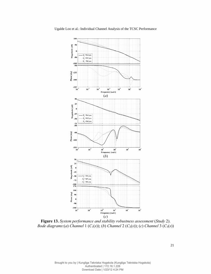
The synchronous generator – TCSC system assuming a varying transmission distance, but keeping a fixed amount of series compensation, is studied in this section. The series compensation value is kept at XTCSC = –0.2 p.u. The controller (23) is used, where kTCSC = –1 for Xt = 0.4 p.u., kTCSC = –3/4 for Xt = 0.5 p.u., and kTCSC = –1/2 for Xt = 0.6 p.u. The control system performance and robustness measures are presented in figures 12–15.

From figures 12–15, it can be seen that the control system performance is adequate for all operating conditions, even for the case of a long transmission line (Xt = 0.6 p.u.) provided series compensation is available. Nevertheless, the performance improves very substantially when the tie-line reactance value is small, regardless of the value of series compensation. It can be seen that an increase in the tie-line reactance value will increase channel coupling, decreasing stability robustness and performance. This confirms previous statements in connection with the analysis of the MSFs studied in earlier sections of this paper. It should be noticed that, similarly to the previous study, channel C3(s) is non-minimum phase since γ3(s) circles the point (1,0) twice in a clockwise direction for all operating conditions.

4. TCSC influence on the system

The control system characteristics are investigated to assess the influence that the TCSC exerts on the system. The TCSC is used to decrease the electrical length of the transmission line in order to boost active power transfer. A high value of tie-line reactance Xt = 0.6 p.u. is considered. When in operation, the TCSC provides a 33.33% of series compensation (XTCSC = –0.2 p.u.). The system operating conditions can be found in Table A4.3 of Appendix 4.

19




(a)

(b)

(c) Figure 12. System performance (Study 2). Step response of: (a) Channel 1

(Tc1(s)); (b) Channel 2 (Tc2(s)); (c) Channel 3 (Tc3(s))

20


DOI: 10.2202/1553-779X.2190



(a)

(b)

(c) Figure 13. System performance and stability robustness assessment (Study 2).

Bode diagrams:(a) Channel 1 (C1(s)); (b) Channel 2 (C2(s)); (c) Channel 3 (C3(s))

21




(a)

(b)

(c) Figure 14. Stability robustness assessment (Study 2). Bode diagrams: (a) k1g11(s);

(b) k2g22(s); (c) k3g33(s)

22


DOI: 10.2202/1553-779X.2190



(a)

(b)

(c) Figure 15. Structural robustness assessment (Study 2). Nyquist diagrams:

(a) γ1(s); (b) γ2(s); (c) γ3(s)

23




Figure 16 shows the relevant MSFs with and with no presence of TCSC. MSF Γ2_3(s) gives a measure of coupling between channels of the synchronous generator C1(s) –speed– and C2(s) –voltage– in Multiple Channel M12(s) when a TCSC is used. On the other hand, γa(s) provides the coupling measure for the synchronous generator when no TCSC is considered. It can be seen that both Γ2_3(s) and γa(s) have a similar frequency response – that is, the dynamical structure is preserved. However, coupling is significantly lower and the structural robustness measures (in terms of gain and phase margins) increase whenever the TCSC is used. Notice that the magnitude peak is moved on to the higher frequencies when the TCSC is included.

(a)

(b) Figure 16. Assessment of γa(s) vs Γ2_3(s). (a) Nyquist plot; (b) Bode plot

The performance of the synchronous generator, with no TCSC, is compared with that given by the system where one TCSC is included. A controller for the 2×2 system with no TCSC channel is

24


DOI: 10.2202/1553-779X.2190



( ) ( )( )

( )( )

( )211

222

5.75 6.1 165.50 14 0.43diag

0 5

s sk s ss

k s s s s

⎡ ⎤+ +⎡ ⎤ +⎢ ⎥= =⎢ ⎥ +⎢ ⎥⎣ ⎦ ⎣ ⎦

1aK (24)

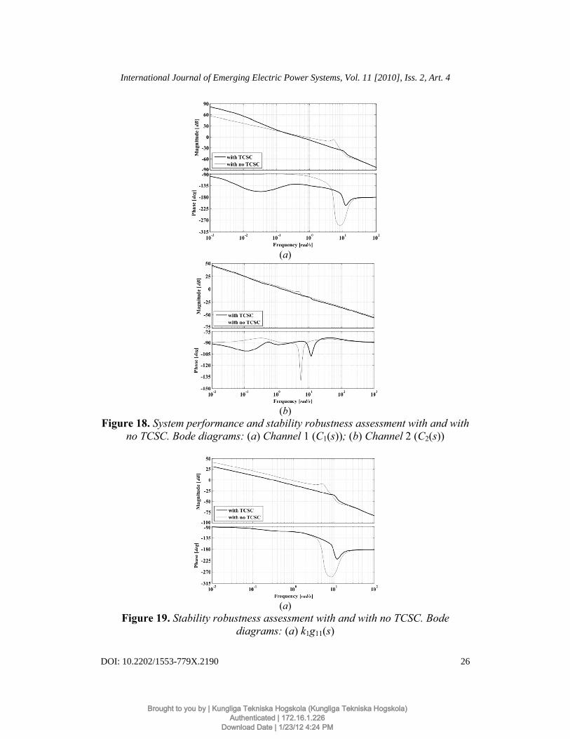
Notice that controller (24) is exactly the same as (23) but with no TCSC channel. When the TCSC is employed, the constant kTCSC = –1/2 in the impedance control loop. Figures 17–20 show the performance of the closed-loop control system (terminal voltage and speed channels) and robustness assessment with and with no TCSC.

(a)

(b) Figure 17. System performance with and with no TCSC. Step response of:

(a) Channel 1 (Tc1(s)); (b) Channel 2 (Tc2(s))

25




(a)

(b) Figure 18. System performance and stability robustness assessment with and with

no TCSC. Bode diagrams: (a) Channel 1 (C1(s)); (b) Channel 2 (C2(s))

(a) Figure 19. Stability robustness assessment with and with no TCSC. Bode

diagrams: (a) k1g11(s)

26


DOI: 10.2202/1553-779X.2190



(b) Figure 19. Stability robustness assessment with and with no TCSC. Bode

diagrams: (b) k2g22(s)

(a)

(b) Figure 20. Structural robustness assessment with and with no TCSC. Nyquist

diagrams: (a) γah2(s) vs γ1(s); (b) γah1(s) vs γ2(s)

27




From figure 17, it can be seen that the system tends to be oscillatory whenever the TCSC is not used. However, the Bode diagram of C1(s) in figure 18 shows an important detrimental effect that the TCSC introduces into the system: a weakening of stability robustness – which is proof that C3(s) significantly couples with the speed channel C1(s). However, an important positive effect of the inclusion of the TCSC can be appreciated in the Bode diagram of C2(s) shown in figure 18: the switch-back characteristic, quite prominent with no TCSC, reduces considerably and moves on to the higher frequencies. Also, the use of the TCSC considerably improves the structural robustness in the voltage channel C2(s), even though it tends to worsen the speed channel C1(s) (figure 19). In fact, the MSFs γi(s) lag γahi(s) by 180 deg under all operating conditions (figure 20).

5. Extreme cases of TCSC operation

Although the TCSC has two distinctive regions of operation, it is common practice to operate it only in its capacitive region. This enables the effective impedance of the transmission line to be shortened very smoothly by suitably changing the thyristor’s firing angle in order to increase active power flows through the compensated transmission line.

The TCSC impedance characteristic of the Kayenta installation (Christl, et al., 1992), shown in figure 4, starts its capacitive region of operation at firing angles greater than 142.531°. Moreover, the closer the firing angle is to the resonance point, the higher the amount of series compensation that can be achieved. However, series compensation is limited among other things by the amount of reactive power that the synchronous machine is able to inject or absorb into the system. On the other hand, for values of firing angle smaller than the resonant point, the TCSC will act in its inductive region. Both cases will be examined in this section.

5.1. Maximum capacitive compensation

Consider the operating conditions given in Table A4.4 of Appendix 4. A large value of tie-line reactance Xt = 0.6 p.u. is considered. Three cases of series compensation are examined while keeping the active power constant: 70% (XTCSC= –0.42 p.u.), 80% (XTCSC = –0.48 p.u.) and 83.33% (XTCSC = –0.5 p.u.). As the amount of compensation increases, the reactive power absorbed by the synchronous machine increases and the power factor tends to fall. At a compensation level of 83.33%, the reactive power value is very high. Notice that for the required firing angles, the variations of XTCSC are quite large even for a small variation in the controlling firing angle; therefore, the value of F(α) = ∂XTCSC / ∂α tends to considerably increase with the amount of compensation. The

28


DOI: 10.2202/1553-779X.2190



system performance is assessed for cases when no TCSC and TCSC is included, using the same operating conditions, and comparisons are drawn.

In order to assess the coupling between channels of the synchronous generator (speed and terminal voltage), Figure 21 shows the relevant MSFs associated with the operating conditions of Table A4.4 (Appendix 4) – that is, MSFs Γ2_3(s) in the TCSC upgraded-system and γa(s) for the system with no TCSC.

(a)

(b) Figure 21. Assessment of MSFs for high compensation values. (a) Nyquist plot;

(b) Bode plot

From figure 21, it can be seen that the inclusion of a TCSC providing high compensation values reduces very dramatically the coupling between individual channels C1(s) and C2(s) compared to the case with no TCSC. Notice that the characteristic peak exhibited by the MSFs is shifted to higher frequencies and becomes considerably attenuated. The decrease of tie-line reactance values is reflected in the control system design by an increase of bandwidth.

29




The control system design is carried out as before, using controller (23). For instance, if an impedance control loop gain kTCSC = –0.2 for 70% of compensation is used, and –0.072 for 80% and –0.0468 for 83.33%, a control system design offering an adequate performance and robustness measures can be arrived at (not shown). Nevertheless, it should be pointed out that for such operating conditions the system is minimum-phase. This is evidenced by noticing that MSFs γ3(s) no longer encircles the point (1,0), as shown in figure 22 – in fact, the gain margins tend to increase with the series compensation as the Nyquist trajectories tend to pass farther away from the critical point. In the case of a transmission line of Xt = 0.6 p.u., a series compensation of over 70% will ensure a minimum phase system. Such a condition is of great interest and relevance. Among the most obvious benefits are a higher bandwidth in the TCSC control loop channel even for high values of transmission line reactance and considerably high compensation levels.

Figure 22. Structural robustness assessment. Nyquist diagrams of γ3(s)

In connection with the previous result, it is of interest to assess the minimum phase condition in a TCSC upgraded-system while considering different values of tie-line reactances. The operating conditions given in Table A4.5 (Appendix 4) are used to such an end. In figure 23, the TCSC impedance characteristic is shown to study these cases. It is evident that the higher the amount of series compensation required, the closer the firing angle is to the resonant point. Moreover, the higher the value of the tie-line reactance is, the higher the amount of series compensation required to ensure a minimum phase condition.

Figure 24 shows MSFs Γ2_3(s) associated with the operating conditions of Table A4.5 (Appendix 4). Individual Channels C1(s) (speed) and C2(s) (terminal voltage) of the synchronous generator are totally decoupled by the inclusion of the TCSC, which is an expected result. Notice that all plots are quite similar regardless of the value of tie-line reactance and percentage of compensation used.

30


DOI: 10.2202/1553-779X.2190



Figure 23. TCSC impedance characteristic (XTCSC) near the resonance point

(a)

(b) Figure 24. Assessment of Γ2_3(s) for compensation values ensuring minimum

phase systems: (a) Nyquist plot; (b) Bode plot

31




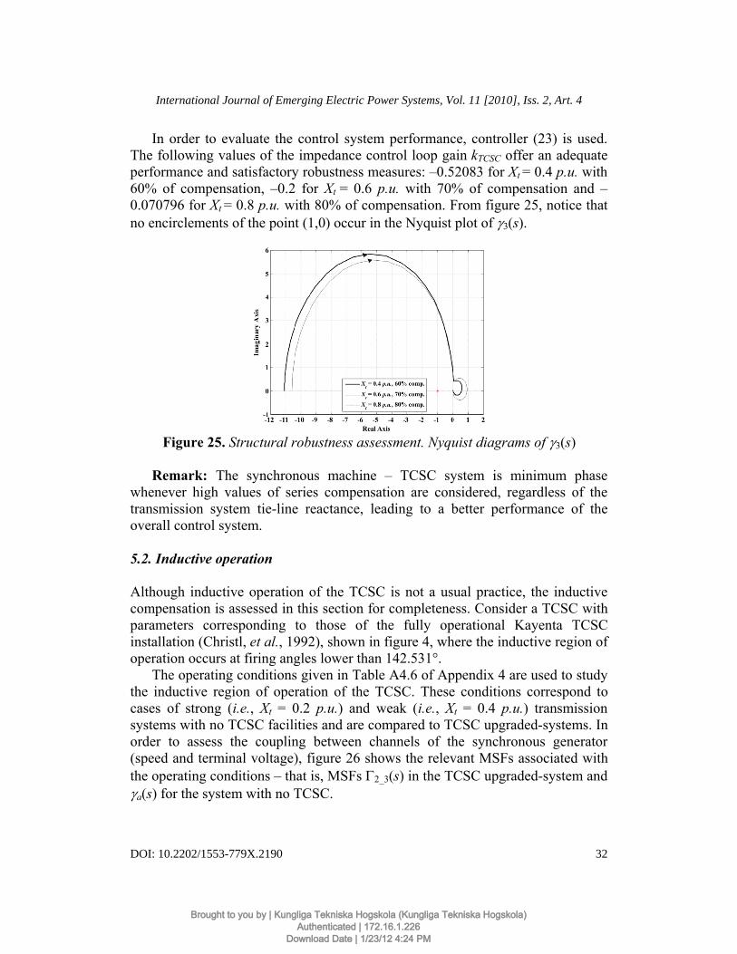
In order to evaluate the control system performance, controller (23) is used. The following values of the impedance control loop gain kTCSC offer an adequate performance and satisfactory robustness measures: –0.52083 for Xt = 0.4 p.u. with 60% of compensation, –0.2 for Xt = 0.6 p.u. with 70% of compensation and –0.070796 for Xt = 0.8 p.u. with 80% of compensation. From figure 25, notice that no encirclements of the point (1,0) occur in the Nyquist plot of γ3(s).

Figure 25. Structural robustness assessment. Nyquist diagrams of γ3(s)

Remark: The synchronous machine – TCSC system is minimum phase whenever high values of series compensation are considered, regardless of the transmission system tie-line reactance, leading to a better performance of the overall control system.

5.2. Inductive operation

Although inductive operation of the TCSC is not a usual practice, the inductive compensation is assessed in this section for completeness. Consider a TCSC with parameters corresponding to those of the fully operational Kayenta TCSC installation (Christl, et al., 1992), shown in figure 4, where the inductive region of operation occurs at firing angles lower than 142.531°.

The operating conditions given in Table A4.6 of Appendix 4 are used to study the inductive region of operation of the TCSC. These conditions correspond to cases of strong (i.e., Xt = 0.2 p.u.) and weak (i.e., Xt = 0.4 p.u.) transmission systems with no TCSC facilities and are compared to TCSC upgraded-systems. In order to assess the coupling between channels of the synchronous generator (speed and terminal voltage), figure 26 shows the relevant MSFs associated with the operating conditions – that is, MSFs Γ2_3(s) in the TCSC upgraded-system and γa(s) for the system with no TCSC.

32


DOI: 10.2202/1553-779X.2190



(a)

(b) Figure 26. Assessment of MSFs for inductive compensation. (a) Nyquist plot;

(b) Bode plot

Figure 26 formally shows that the inclusion of the TCSC operating in its inductive region impairs system operation; that is, a strong transmission system becomes weak. Whenever the TCSC is included into a strong transmission system, it becomes more coupled. The characteristic peak featured by the MSF γa(s) of the synchronous machine with no TCSC is shifted to higher frequencies in Γ2_3(s) of the TCSC upgraded-system, but in this case its magnitude is amplified. The effect of a TCSC with XTCSC = 0.2 p.u. into a transmission tie-line of Xt = 0.2 p.u. is equivalent to having a weaker transmission system with no TCSC and a tie-line of Xt = 0.4 p.u., with the only difference being the frequency at which the peak magnitude occurs.

In terms of control system design, the increase in the effective reactance of the transmission line will be reflected in a bandwidth reduction in order to obtain an adequate performance, which can be assessed using controller (23) with values of gain kTCSC given as follows: kTCSC = –4.78 for –25% compensation, kTCSC = –1.444

33




for –50% compensation and kTCSC = –0.375 for –100% compensation. The resulting performance and robustness are adequate (not shown). Nonetheless, because of the previously stated reasons, operation of the TCSC in its inductive region is rare since it provides no obvious benefit to system operation.

6. Conclusion

In this paper a small-signal stability assessment and multivariable control system analysis and design of the synchronous generator – TCSC system has been carried out. The parameters of the fully operational and already installed TCSC in Kayenta have been used. By means of the ICAD framework, fundamental analyses have been carried out explaining the generator dynamics as affected by the TCSC. Simulation results obtained are in agreement with system behaviour observed in practice.

It is formally shown that the addition of the TCSC when operated in its capacitive region improves the dynamical performance of the synchronous machine very substantially, decreasing the electrical distance and therefore considerably reducing the awkward switch-back characteristic exhibited by synchronous generators. Although an effective modulation of the tie-line reactance and a better regulation of power flows are available, it should be noticed that the inclusion of a TCSC brings fragility on to the global system on two counts: (i) the system becomes non-minimum phase (except for extreme compensation cases), limiting its potential performance; (ii) the TCSC impedance control loop introduces adverse dynamics in terms of cross-coupling, particularly in the speed channel of the synchronous machine. The minimum phase condition brought about by high compensation levels opens the door to some interesting debate: What is the best TCSC operating region, along its impedance characteristic? Also, it is formally shown that the operation of the TCSC in its inductive region impairs system performance.

All these key points of TCSC operation have been elucidated only after application of ICAD and may not have been revealed, at least not as emphatically, by other analysis methods such as block diagram representations and eigenanalysis.

Appendix 1. System coefficients and transfer functions

The parameters and transfer functions of equations (1)–(7) are given by

2200

1 0 0 0 0'' ''qd

tq d td qd q

VVK i V i V∞∞

∞ ∞= + − +Λ Λ

34


DOI: 10.2202/1553-779X.2190



02 ''

d

d

VK ∞=

Λ

02 ''

qd

q

VK ∞=

Λ

( ) 0 00 01 '' ''

tq qtd dTCSC

d q

i Vi VK F α ∞∞

⎡ ⎤= − ⋅ +⎢ ⎥

Λ Λ⎢ ⎥⎣ ⎦

'' ''d d t TCSCX X XΛ = + +

'' ''q q t TCSCX X XΛ = + +

'' ''0 00 0

5 '' ''0 0

q q tqtd d d

t tq d

X V ee X VK

e e∞ ∞

⎡ ⎤= ⋅ − ⋅⎢ ⎥

Λ Λ⎢ ⎥⎣ ⎦

06 ''

0

tq t TCSC

t d

e X XK

e⎡ ⎤+

= ⋅⎢ ⎥Λ⎣ ⎦

06 ''

0

td t TCSCd

t q

e X XK

e⎡ ⎤+

= ⋅⎢ ⎥Λ⎢ ⎥⎣ ⎦

( )'' ''

0 00 03 '' ''

0 0

q tq tqtd d tdTCSC

t tq d

X i ee X iK F

e eα

⎡ ⎤= − ⋅ ⋅ − ⋅⎢ ⎥

Λ Λ⎢ ⎥⎣ ⎦

0 00 05 '' ''

0 0

tq qtd dn

t td q

i Vi VK

i i∞∞

⎡ ⎤= ⋅ + ⋅⎢ ⎥

Λ Λ⎢ ⎥⎣ ⎦

06 ''

0

1tdn

t d

iK

i⎡ ⎤

= ⋅⎢ ⎥Λ⎣ ⎦

06 ''

0

1tqdn

t q

iK

i⎡ ⎤

= ⋅⎢ ⎥Λ⎢ ⎥⎣ ⎦

( )22

003 '' ''

0 0

1 1tqtdTCSC n

t td q

iiK F

i iα

⎡ ⎤= − ⋅ ⋅ + ⋅⎢ ⎥

Λ Λ⎢ ⎥⎣ ⎦

35




( )( )

( ){ } { }

'' ''0

3 '' '' ' ' ' ' '' '' 20 0 0 0

1d d

d d d d d d d d d d

sK s

X X s s

τ

τ τ τ τ

⎡ ⎤Λ +⎢ ⎥= ⎢ ⎥⎡ ⎤Λ + Λ + − + Λ + Λ⎢ ⎥⎣ ⎦⎣ ⎦

( )( ) ( ) ( ){ }

( ){ } { }

'' ' ' '' '' '0 0 0

4 '' '' ' ' ' ' '' '' 20 0 0 0

d d d d d d d d d

d d d d d d d d d d

V X X X X X X sK s

X X s s

τ τ

τ τ τ τ

∞⎡ ⎤⎡ ⎤− + − + −⎣ ⎦⎢ ⎥= ⎢ ⎥⎡ ⎤Λ + Λ + − + Λ + Λ⎢ ⎥⎣ ⎦⎣ ⎦

( ) ( )( ) ( ) ( ){ }

( ){ } { }

'' ' ' '' '' '0 0 0

2 '' '' ' ' ' ' '' '' 20 0 0 0

td d d d d d d d d

TCSC

d d d d d d d d d d

i X X X X X X sK s F

X X s s

τ τα

τ τ τ τ

⎡ ⎤⎡ ⎤− + − + −⎣ ⎦⎢ ⎥= − ⋅ ⎢ ⎥⎡ ⎤Λ + Λ + − + Λ + Λ⎢ ⎥⎣ ⎦⎣ ⎦

( ) 44 ''1

dd

q

CK s

sτ=

+

( ) 22 ''1

TCSC dTCSC d

q

CK s

sτ=

+

' 'd d t TCSCX X XΛ = + +

d d t TCSCX X XΛ = + +

( )''0

4q q q

dq

X X VC ∞− ⋅

=Λ

( )( )''

02

q q tqTCSC d

q

X X iC F α

⎡ ⎤− ⋅⎢ ⎥= −

Λ⎢ ⎥⎣ ⎦

q q t TCSCX X XΛ = + +

'''' ''

0q

q qq

τ τ⎛ ⎞Λ

= ⎜ ⎟⎜ ⎟Λ⎝ ⎠

36


DOI: 10.2202/1553-779X.2190



Appendix 2. Individual elements of the transfer matrix G(s) of the linearized synchronous generator – TCSC system model

The individual elements of the transfer matrix G(s) defined in (10) are given by

( )( )( )

( )

2 ''

11

1d qEs Fs s sg s

den s

τ+ + Λ +=

( )( )( )

( )

'' '' ''2 0

12

1 1d d qK s s sg s

den s

τ τΛ + += −

( )( )( ) ( )( ) ( )

( )

2 '' '' 21 2 2 2

13

1 1TCSC d q q d TCSC d dK Es Fs s K I B Cs s K C Es Fs sg s

den s

τ τ⎡ ⎤+ + Λ + − + + − + + Λ⎣ ⎦= −

( )( )( ) ( )( ) ( )

( )

2 '' '' 20 5 6 0 6 4

21

1 1d q d q d d dK Es Fs s K V B Cs s K C Es Fsg s

den s

ω τ τ∞⎡ ⎤+ + Λ + − + + + + + Λ⎣ ⎦=

( )( ) ( )( ) ( ) ( )( ){ }

( )

'' '' '' '' ''0 6 6 1 2 4 2 5 6 4 0

22

1 1 2 1 1d d q q d d q d ds K s Hs D s K s K K C K s K K Cg s

den s

τ τ τ τ ω⎡ ⎤ ⎡ ⎤Λ + + + + + − − + +⎣ ⎦ ⎣ ⎦=

( )( ) ( ) ( ) ( )( ){ }

( )

( ) ( ) ( ) ( )( ){ }( )

( ) ( ) ( )

2 '' ''3 6 2 6

23

2 ''0 6 1 2 4 1 2 5 2 4 3 1 3 5 1

''0 2 5 1 6 0 6 1 2

2 1 1

1

1

d q TCSC d TCSC d q

d d TCSC d d TCSC d TCSC d d TCSC q TCSC TCSC

q d TCSC

Hs D Es Fs s K K C K I B Cs s sg s

den s

Es Fs K K C C K K K C C K s K K K K

den s

B Cs s I K K K K V K K K K

τ τ

ω τ

ω τ ∞

⎡ ⎤+ + + Λ + + − + +⎣ ⎦= +

⎡ ⎤+ + Λ − + − + + −⎣ ⎦+ +

+ + − + −+

( ) ( )( ){ }( )

3 4 2 0 2 6 2 6TCSC d TCSC d d d dIC C V K K K K

den s

∞⎡ ⎤⎡ ⎤ + − +⎣ ⎦⎣ ⎦

( )( )( ) ( ) ( ) ( )

( )

2 '' '' 20 5 6 0 6 4

31

1 1n d q n d q dn d dK Es Fs s K V B Cs s K C Es Fsg s

den s

ω τ τ∞⎡ ⎤+ + Λ + − + + − + + Λ⎣ ⎦=

( )( ) ( )( ) ( ) ( )( ){ }

( )

'' '' '' '' ''0 6 6 1 2 4 2 5 6 4 0

32

1 1 2 1 1d d n q n q d d q n dn ds K s Hs D s K s K K C K s K K Cg s

den s

τ τ τ τ ω⎡ ⎤ ⎡ ⎤Λ + + + + + − − + −⎣ ⎦ ⎣ ⎦=

37




( )( ) ( ) ( ) ( ) ( ){ }

( )

( ) ( ) ( ) ( ) ( ){ }( )

( ) ( ) ( )

2 '' ''3 6 2 6

33

2 ''0 6 4 1 1 2 2 5 2 4 3 1 3 5 1

''0 2 5 1 6 0 6

2 1 1

1

1

d q TCSC n dn TCSC d n q

d dn d TCSC TCSC d d n TCSC d d TCSC n q TCSC n n TCSC

q n n d

Hs D Es Fs s K K C K I B Cs s sg s

den s

Es Fs K C K K C K K C C K s K K K K

den s

B Cs s I K K K K V K

τ τ

ω τ

ω τ ∞

⎡ ⎤+ + + Λ + − − + +⎣ ⎦= +

⎡ ⎤+ + Λ − + − + + −⎣ ⎦+ +

+ + − ++

( ) ( ) ( ){ }( )

1 2 3 4 2 0 2 6 2 6n TCSC TCSC n d TCSC d d d n dnK K K IC C V K K K K

den s

∞⎡ ⎤⎡ ⎤− + − −⎣ ⎦⎣ ⎦

where

( ) ( )( ) ( )( ) ( )2 '' '' 21 0 2 0 0 2 4 0( ) 2 1 1d q d q d d dden s Hs D s K Es Fs s K V B Cs s K C Es Fsω τ ω τ ω∞= + + + + Λ + − + + − + + Λ⎡ ⎤⎣ ⎦

''d dB X X= −

( ) ( )' ' '' '' '0 0d d d d d dC X X X Xτ τ= − + −

' '' ''0 0d d dE τ τ= Λ

( )'' '' ' ' '0 0d d d d d dF X Xτ τ⎡ ⎤= Λ + − + Λ⎣ ⎦

( )0tdI i F α= −

Appendix 3. Synchronous Machine and TCSC Parameters

Table A3.1. Synchronous machine parameters

Variable Value

Xd 1.445 p.u. X’

d 0.316 p.u. X’’

d 0.179 p.u.

τ’d0 5.26 s

τ’’d0 0.028 s

Xq 0.959 p.u. X’’

q 0.158 p.u.

τ’q0 / τ’’

q0 0.159 s

Ra 0 D 0 H 4.27 s f0 50 Hz

38


DOI: 10.2202/1553-779X.2190



Table A3.2. TCSC parameters Variable Value

XL 1.625 x 10-3 p.u. XC 9.375 x 10-3 p.u.

Appendix 4. System operating conditions

Table A4.1. System operating condition for Study 1 Variable Case 1

50% comp. Case 2

25% comp. Case 3

10% comp. Pg 0.736 p.u. 0.736 p.u. 0.736 p.u. Qg 0.4307 p.u. 0.3082 p.u. 0.262 p.u. PF 0.91958 0.94558 0.95065 δ0 30° 30° 30°

|V∞0| 1 p.u. 1 p.u. 1 p.u. ∠ V∞0 60° 60° 60° |et0| 1.05 p.u. 1.05 p.u. 1.05 p.u. ∠ et0 68.055° 72.139° 74.615°

|it0| / |I∞0| 0.76225 p.u. 0.74129 p.u. 0.73734 p.u. ∠ it0 / ∠ I∞0 44.92° 53.151° 56.539°

XTCSC –0.2 p.u. –0.1 p.u. –0.04 p.u.α 143.08° 143.65° 145.47°

∂XTCSC / ∂α 20.431 4.9546 0.71622 Xt 0.4 p.u. 0.4 p.u. 0.4 p.u.

Xtotal 0.2 p.u. 0.3 p.u. 0.36 p.u.

Table A4.2. System operating condition for Study 2 Variable Case 1

50% comp. Case 2

40% comp. Case 3

33.3% comp.Pg 0.736 p.u. 0.736 p.u. 0.736 p.u. Qg 0.4307 p.u. 0.3633 p.u. 0.345 p.u. PF 0.91958 0.94557 0.95204 δ0 30° 35° 40°

|V∞0| 1 p.u. 1 p.u. 1 p.u.∠ V∞0 60° 55° 50° |et0| 1.05 p.u. 1.05 p.u. 1.05 p.u.∠ et0 68.055° 67.135° 66.278°

|it0| / |I∞0| 0.76225 p.u. 0.7413 p.u. 0.73626 p.u.∠ it0 / ∠ I∞0 44.92° 48.144° 48.461°

XTCSC –0.2 p.u. –0.2 p.u. –0.2 p.u.α 143.08° 143.08° 143.08°

∂XTCSC / ∂α 20.431 20.431 20.431 Xt 0.4 p.u. 0.5 p.u. 0.6 p.u.

Xtotal 0.2 p.u. 0.3 p.u. 0.4 p.u.

39




Table A4.3. System operating condition for comparison with and with no TCSC

Value Value Variable with TCSC with no

TCSC Variable with TCSC with no

TCSC Pg 0.736 p.u. 0.736 p.u. |it0| / |I∞0| 0.73626 p.u. 0.74022 p.u.

Qg 0.345 p.u. 0.2498 p.u. ∠ it0 / ∠ I∞0 48.461° 56.123°

PF 0.95204 0.94695 Efd0 1.6668 p.u. 1.6098 p.u.

δ0 40° 40° XTCSC –0.2 p.u. –

|V∞| 1 p.u. 1 p.u. α 143.08° –

∠ V∞ 50° 50° ∂XTCSC / ∂α 20.431 –

|et0| 1.05 p.u. 1.05 p.u. Xt 0.6 p.u. 0.6 p.u.

∠ et0 66.278° 74.871° Xtotal 0.4 p.u. 0.6 p.u.

Table A4.4. System operating condition for maximum compensation

Variable No TCSC Xt = 0.6 p.u.

Case 1 70% comp.

Case 2 80% comp.

Case 3 83.33% comp.

Pg 0.736 p.u. 0.736 p.u. 0.736 p.u. 0.736 p.u.

Qg 0.2498 p.u. 0.5884 p.u. 0.8 p.u. 0.9333 p.u.

PF 0.94695 0.90858 0.84348 0.80159

δ0 30° 30° 30° 30°

|V∞0| 1 p.u. 1 p.u. 1 p.u. 1 p.u.

∠ V∞0 60° 60° 60° 60°

|et0| 1.05 p.u. 1.05 p.u. 1.05 p.u. 1.05 p.u.

∠ et0 84.871 67.246° 64.823° 64.023°

|it0| / |I∞0| 0.74022 p.u. 0.77148 p.u. 0.83102 p.u. 0.87446 p.u.

∠ it0 / ∠ I∞0 66.123° 42.556° 32.334° 27.233°

XTCSC - –0.42 p.u. –0.48 p.u. –0.5 p.u.

α - 142.7918° 142.7589° 142.7498°

∂XTCSC / ∂α - 91.349 119.5 129.6

Xt 0.6 p.u. 0.6 p.u. 0.6 p.u. 0.6 p.u.

Xtotal 0.6 p.u. 0.18 p.u. 0.12 p.u. 0.1 p.u.

40


DOI: 10.2202/1553-779X.2190



Table A4.5. System operating condition providing minimum phase systems

Variable Case 1 60% comp.

Case 2 70% comp.

Case 3 80% comp.

Pg 0.736 p.u. 0.736 p.u. 0.736 p.u. Qg 0.5171 p.u. 0.5884 p.u. 0.76275 p.u. PF 0.89371 0.90858 0.89328

δ0 30° 30° 30°

|V∞0| 1 p.u. 1 p.u. 1 p.u.

∠ V∞0 60° 60° 60° |et0| 1.05 p.u. 1.05 p.u. 1.05 p.u.

∠ et0 66.441° 67.246° 66.446° |it0| / |I∞0| 0.78432 p.u. 0.77148 p.u. 0.78422 p.u.

∠ it0 / ∠ I∞0 39.784° 42.556° 39.803° XTCSC –0.24 p.u. –0.42 p.u. –0.64 p.u.

α 142.9905° 142.7918° 142.7015°

∂XTCSC / ∂α 29.52 91.349 212.89

Xt 0.4 p.u. 0.6 p.u. 0.8 p.u.Xtotal 0.16 p.u. 0.18 p.u. 0.16 p.u.

Table A4.6. System operating condition for inductive operation

Variable No TCSC Xt = 0.2 p.u.

Case 1 –25% comp.

Case 2 –50% comp.

Case 3 –100% comp.

No TCSC Xt = 0.4 p.u.

Pg 0.736 p.u. 0.736 p.u. 0.736 p.u. 0.736 p.u. 0.736 p.u. Qg 0.3143 p.u. 0.2469 p.u. 0.1983 p.u. 0.1283 p.u. 0.2365 p.u. PF 0.91965 0.93682 0.94559 0.95206 0.95206

δ0 30° 32.5° 35° 40° 40° |V∞0| 1 p.u. 1 p.u. 1 p.u. 1 p.u. 1 p.u.

∠ V∞0 60° 57.5° 55° 50° 50° |et0| 1.05 p.u. 1.05 p.u. 1.05 p.u. 1.05 p.u. 1.05 p.u.

∠ et0 68.0589 67.596° 67.139° 66.273° 66.2829

|it0| / |I∞0| 0.76219 p.u. 0.74822 p.u. 0.74129 p.u. 0.73625 p.u. 0.73625 p.u.

∠ it0 / ∠ I∞0 44.935° 47.112° 48.15° 48.455° 48.469° XTCSC - 0.05 p.u. 0.1 p.u. 0.2 p.u. -

α - 140.45° 141.46° 141.99° -

∂XTCSC / ∂α - 1.4418 5.5067 21.464 -

Xt 0.2 p.u. 0.2 p.u. 0.2 p.u. 0.2 p.u. 0.4 p.u. Xtotal 0.2 p.u. 0.25 p.u. 0.3 p.u. 0.4 p.u. 0.4 p.u.

41




Appendix 5. A note on m×m systems under the ICAD framework

In general, the i-th Individual Channel Ci(s) in an m×m system has the open-loop SISO transmittance

( ) ( )1i i ii iC s k g γ= − (A.1)

and

( ) / ii i iis gγ = − G G (A.2)

subjected to disturbances

( ) / ii id s = − R G (A.3)

where i = 1,…,m. In order to construct (A.2) and (A.3), let matrix G be defined as

( )

11 1 12 1

21 22 2 2

1 2

//

/

m

m

m m mm m

g h g gg g h g

s

g g g h

⎡ ⎤⎢ ⎥⎢ ⎥=⎢ ⎥⎢ ⎥⎣ ⎦

G

L

L

M M M

L

(A.4)

and

( ) ( )/ 1i i ii i iih s k g k g= + (A.5)

Matrix 1 2 ... ri i iG is defined as a matrix obtained from G by eliminating the i1-th row and column, then the i2-th row and column and so on, up to the ir-th row and column. Similarly, matrix 1 2 ... ri i i

jG is defined as a matrix obtained by setting the diagonal element gjj/hj of G to zero before eliminating the rows and columns as in the definition of 1 2 ... ri i iG . Ri is defined as the matrix obtained by replacing the i-th column of G by r and setting ri to zero. In fact, a relationship between Γi(s) (13) and γi(s) (A.2) exists:

42


DOI: 10.2202/1553-779X.2190



( ) ( ) ( ) ( )

( ) ( )

( ) ( )

12 1 2 1

1 2 1

1 2

|0

1

mi i h i h i h

i

imi i

s s

h h hs

h h h

γ

γ

+ = + = = =

−

+ +

Γ =

= = = ==

= = = =

K L

L

L

(A.6)

For detailed information on ICAD for m×m systems, the reader is referred to the work of Leithead and O’Reilly (1992).

References

Angquist L., Lundin B. and Samuelsson J. “Power Oscillation Damping using Controlled Reactive Power Compensation: a Comparison between Series and Shunt Approaches.” IEEE Transactions on Power Systems, 8(2), pp. 687-699, 1993.

Aree P. Small Signal Stability Modelling and Analysis of Power Systems with Electronically Controlled Compensation. PhD Thesis. Department of Electronics and Electrical Engineering, University of Glasgow, Scotland, UK, 2000.

Aree P. and Acha E. “Block diagram model for fundamental studies of a synchronous generator–static VAr compensator system.” IEE Proceedings on Generation, Transmission and Distribution, 146(5), pp. 507-514, 1999.

Christl N., Hedin R., Sadek K., Lutzelberger P., Krause P.E., McKenna S.M., Montoya A.H. and Togerson D. “Advanced Series Compensation (ASC) with Thyristor Controlled Impedance.” Proceedings of International Conference of Large High Voltage Electric Systems (CIGRE), 14/37/38-05, Paris, 1992.

Hammons T.J. and Winning D.J. “Comparison of synchronous machine models in the study of the transient behaviour of electrical systems.” Proceedings IEE,118(10), pp. 1442-1458, 1971.

Helbing S.G. and Karady G.G. “Investigations of an Advanced Form of Series Compensation.”IEEE Transactions on Power Delivery,9(2), pp. 939-947,1994.

IEEE/CIGRE. “FACTS Overview.” Special Issue, 95-TP-108, IEEE Service Centre, USA, 1995.

43




Iliceto F. and Cinieri E. “Comparative Analysis of Series and Shunt Compensation Control Schemes for AC Transmission Systems.” IEEE Transactions on Power Apparatus and Systems, 96(1), pp. 1819-1830, 1977.

Jancke G., Fahlen, N. and Nerf O. “Series Capacitor in Power System.” IEEE Transactions on Power Apparatus and Systems, 94, pp. 915-925, 1975.

Kundur P., Rogers, G.J., Wong D.Y., Wang L. and Lauby M.G. “A Comprehen-sive Computer Program Package for Small Signal Stability Analysis of Power Systems” IEEE Transactions on Power Systems, 5(4), pp. 1076-1083, 1990.

Kundur P. Power System Stability and Control. The EPRI Power Systems Engineering Series, McGraw-Hill, 1994.

Leithead, W.E. and O’Reilly, J. “m-input m-output feedback control by individual channel design Part I: Structural issues.” International Journal of Control,56(6), pp. 1347-1397, 1992.

Saidy, M. and Hughes, F.M. “Block diagram transfer function model of a generator including damper windings.” IEE Proceedings on Generation, Transmission and Distribution, 141(6), pp. 599-608, 1994.

Ugalde C.E., Vanfretti L., Licéaga-Castro E. and Acha E. “Synchronous generator modeling and control using the framework of individual channel analysis and design. Part 1.” International Journal of Emerging Electric Power Systems, 8(5), art 4, 2007 (

Ugalde C.E., Acha E., Licéaga-Castro E. and Licéaga-Castro J. “Fundamental Analysis of the Static VAr Compensator Performance Using Individual Channel Analysis and Design.” International Journal of Emerging Electric Power Systems,9(2),art 6,2008 (

Ugalde C.E., Acha E., Licéaga-Castro E. and Vanfretti L. “Fundamental Analysis of the Synchronous – TCSC System using the ICAD Framework.” Proceedings of the 16th Power Systems Computation Conference, Glasgow, Scotland, 2008.

44


DOI: 10.2202/1553-779X.2190



individual channel analysis of the thyristor-controlled - diva portal

Documents