arX

iv:m

ath/

0703

365v

1 [

mat

h.ST

] 1

3 M

ar 2

007

Indicator function and complex coding for

mixed fractional factorial designs 1

Giovanni Pistone

Department of Mathematics - Politecnico di Torino

Maria-Piera Rogantin ∗

Department of Mathematics - Universita di Genova

Abstract

In a general fractional factorial design, the n-levels of a factor are coded by the n-throots of the unity. This device allows a full generalization to mixed-level designs ofthe theory of the polynomial indicator function which has already been introducedfor two level designs by Fontana and the Authors (2000). the properties of orthogonalarrays and regular fractions are discussed.

Key words: Algebraic statistics, Complex coding, Mixed-level designs, Regularfraction, Orthogonal arrays

1 Introduction

Algebraic and geometric methods are widely used in the theory of the de-sign of experiments. A variety of these methods exist: real linear algebra, Zp

arithmetic, Galois Fields GF(ps) arithmetic, where p is a prime number asin Bose (1947). See, e.g., Raktoe et al. (1981) and the more recent books byDey and Mukerjee (1999) and Wu and Hamada (2000).

Complex coding of levels has been used by many authors in various contexts,see e.g. Bailey (1982), Kobilinsky and Monod (1991), Edmondson (1994), Kobilinsky and Monod(1995), Collombier (1996) and Xu and Wu (2001).

∗ Corresponding author.Email addresses: giovanni.pistone@polito.it (Giovanni Pistone),

rogantin@dima.unige.it (Maria-Piera Rogantin).1 Partially supported by the Italian PRIN03 grant coordinated by G. Consonni

Preprint submitted to jspi 17 December 2013

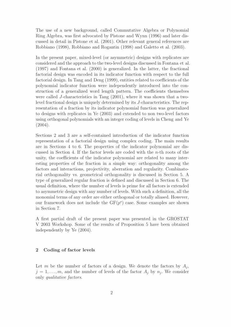
The use of a new background, called Commutative Algebra or PolynomialRing Algebra, was first advocated by Pistone and Wynn (1996) and later dis-cussed in detail in Pistone et al. (2001). Other relevant general references areRobbiano (1998), Robbiano and Rogantin (1998) and Galetto et al. (2003).

In the present paper, mixed-level (or asymmetric) designs with replicates areconsidered and the approach to the two-level designs discussed in Fontana et al.(1997) and Fontana et al. (2000) is generalized. In the latter, the fractionalfactorial design was encoded in its indicator function with respect to the fullfactorial design. In Tang and Deng (1999), entities related to coefficients of thepolynomial indicator function were independently introduced into the con-struction of a generalized word length pattern. The coefficients themselveswere called J-characteristics in Tang (2001), where it was shown that a two-level fractional design is uniquely determined by its J-characteristics. The rep-resentation of a fraction by its indicator polynomial function was generalizedto designs with replicates in Ye (2003) and extended to non two-level factorsusing orthogonal polynomials with an integer coding of levels in Cheng and Ye(2004).

Sections 2 and 3 are a self-contained introduction of the indicator functionrepresentation of a factorial design using complex coding. The main resultsare in Sections 4 to 6. The properties of the indicator polynomial are dis-cussed in Section 4. If the factor levels are coded with the n-th roots of theunity, the coefficients of the indicator polynomial are related to many inter-esting properties of the fraction in a simple way: orthogonality among thefactors and interactions, projectivity, aberration and regularity. Combinato-rial orthogonality vs. geometrical orthogonality is discussed in Section 5. Atype of generalized regular fraction is defined and discussed in Section 6. Theusual definition, where the number of levels is prime for all factors is extendedto asymmetric design with any number of levels. With such a definition, all themonomial terms of any order are either orthogonal or totally aliased. However,our framework does not include the GF(ps) case. Some examples are shownin Section 7.

A first partial draft of the present paper was presented in the GROSTATV 2003 Workshop. Some of the results of Proposition 5 have been obtainedindependently by Ye (2004).

2 Coding of factor levels

Let m be the number of factors of a design. We denote the factors by Aj ,j = 1, . . . , m, and the number of levels of the factor Aj by nj . We consideronly qualitative factors.

2

We denote the full factorial design by D, D = A1 × · · · × Am, and the spaceof all real responses defined on D by R(D).

In some cases, it is of interest to code qualitative factors with numbers, es-pecially when the levels are ordered. Classical examples of numerical codingwith rational numbers aij ∈ Q are: (1) aij = i, or (2) aij = i − 1, or (3)aij = (2i − nj − 1)/2 for odd nj and aij = 2i − nj − 1 for even nj , see(Raktoe et al., 1981, Tab. 4.1). The second case, where the coding takes valuein the additive group Znj

, i.e. integers mod nj , is of special importance. Wecan define the important notion of regular fraction in such a coding. The thirdcoding is the result of the orthogonalization of the linear term in the secondcoding with respect to the constant term. The coding −1, +1 for two-levelfactors has a further property in that the values −1, +1 form a multiplica-tive group. This property was widely used in Fontana et al. (2000), Ye (2003),Tang and Deng (1999) and Tang (2001).

In the present paper, an approach is taked to parallel our theory for two-levelfactors with coding −1, +1. The n levels of a factor are coded by the complexsolutions of the equation ζn = 1:

ωk = exp(

i2π

nk)

, k = 0, . . . , n− 1 . (1)

We denote such a factor with n levels by Ωn, Ωn = ω0, . . . , ωn−1. With sucha coding, a complex orthonormal basis of the responses on the full factorialdesign is formed by all the monomials.

For a basic reference to the algebra of the complex field C and of the n-thcomplex roots of the unity references can be made to Lang (1965); some usefulpoints are collected in Section 8 below.

As α = β mod n implies ωαk = ωβ

k , it is useful to introduce the residue classring Zn and the notation [k]n for the residue of k mod n. For integer α, weobtain (ωk)

α = ω[αk]n. The mapping

Zn ←→ Ωn ⊂ C with k ←→ ωk (2)

is a group isomorphism of the additive group of Zn on the multiplicative groupΩn ⊂ C. In other words,

ωhωk = ω[h+k]n .

We drop the sub-n notation when there is no ambiguity.

We denote by:

• #D: the number of points of the full factorial design, #D =∏m

j=1 nj .• L: the full factorial design with integer coding 0, . . . , nj−1, j = 1, . . . , m,

3

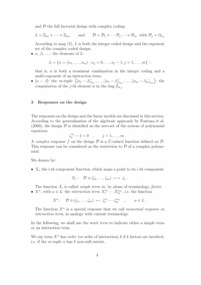
and D the full factorial design with complex coding:

L = Zn1× · · · × Znm

and D = D1 × · · ·Dj · · · × Dm with Dj = Ωnj

According to map (2), L is both the integer coded design and the exponentset of the complex coded design;• α, β, . . . : the elements of L:

L = α = (α1, . . . , αm) : αj = 0, . . . , nj − 1, j = 1, . . . , m ;

that is, α is both a treatment combination in the integer coding and amulti-exponent of an interaction term;• [α − β]: the m-tuple

(

[α1 − β1]n1, . . . , [αj − βj ]nj

, . . . , [αm − βm]nm

)

; the

computation of the j-th element is in the ring Znj.

3 Responses on the design

The responses on the design and the linear models are discussed in this section.According to the generalization of the algebraic approach by Fontana et al.(2000), the design D is identified as the zero-set of the system of polynomialequations

ζnj

j − 1 = 0 , j = 1, . . . , m .

A complex response f on the design D is a C-valued function defined on D.This response can be considered as the restriction to D of a complex polyno-mial.

We denote by:

• Xi; the i-th component function, which maps a point to its i-th component:

Xi : D ∋ (ζ1, . . . , ζm) 7−→ ζi .

The function Xi is called simple term or, by abuse of terminology, factor.• Xα, with α ∈ L: the interaction term Xα1

1 · · ·Xαmm , i.e. the function

Xα : D ∋ (ζ1, . . . , ζm) 7→ ζα1

1 · · · ζαm

m , α ∈ L .

The function Xα is a special response that we call monomial response orinteraction term, in analogy with current terminology.

In the following, we shall use the word term to indicate either a simple termor an interaction term.

We say term Xα has order (or order of interaction) k if k factors are involved,i.e. if the m-tuple α has k non-null entries.

4

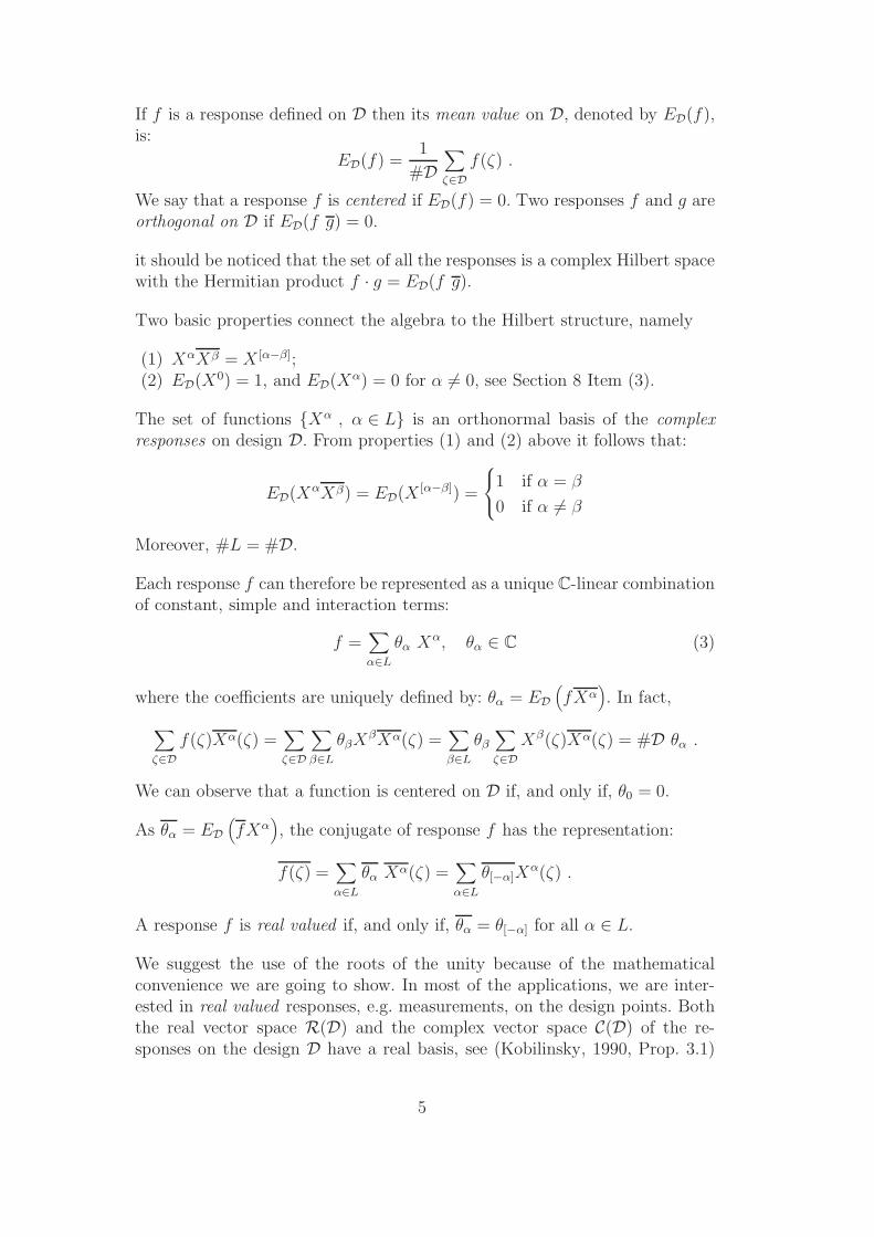
If f is a response defined on D then its mean value on D, denoted by ED(f),is:

ED(f) =1

#D

∑

ζ∈D

f(ζ) .

We say that a response f is centered if ED(f) = 0. Two responses f and g areorthogonal on D if ED(f g) = 0.

it should be noticed that the set of all the responses is a complex Hilbert spacewith the Hermitian product f · g = ED(f g).

Two basic properties connect the algebra to the Hilbert structure, namely

(1) XαXβ = X [α−β];(2) ED(X0) = 1, and ED(Xα) = 0 for α 6= 0, see Section 8 Item (3).

The set of functions Xα , α ∈ L is an orthonormal basis of the complexresponses on design D. From properties (1) and (2) above it follows that:

ED(XαXβ) = ED(X [α−β]) =

1 if α = β

0 if α 6= β

Moreover, #L = #D.

Each response f can therefore be represented as a unique C-linear combinationof constant, simple and interaction terms:

f =∑

α∈L

θα Xα, θα ∈ C (3)

where the coefficients are uniquely defined by: θα = ED

(

fXα)

. In fact,

∑

ζ∈D

f(ζ)Xα(ζ) =∑

ζ∈D

∑

β∈L

θβXβXα(ζ) =

∑

β∈L

θβ

∑

ζ∈D

Xβ(ζ)Xα(ζ) = #D θα .

We can observe that a function is centered on D if, and only if, θ0 = 0.

As θα = ED

(

fXα)

, the conjugate of response f has the representation:

f(ζ) =∑

α∈L

θα Xα(ζ) =∑

α∈L

θ[−α]Xα(ζ) .

A response f is real valued if, and only if, θα = θ[−α] for all α ∈ L.

We suggest the use of the roots of the unity because of the mathematicalconvenience we are going to show. In most of the applications, we are inter-ested in real valued responses, e.g. measurements, on the design points. Boththe real vector space R(D) and the complex vector space C(D) of the re-sponses on the design D have a real basis, see (Kobilinsky, 1990, Prop. 3.1)

5

and Pistone and Rogantin (2005), where a special real basis that is commonto both spaces is computed. The existence of a real basis implies the existenceof real linear models even though the levels are complex.

4 Fractions

A fraction F is a subset of the design, F ⊆ D. We can algebraically describea fraction in two ways, namely using generating equations or the indicatorpolynomial function.

4.1 Generating equations

All fractions can be obtained by adding further polynomial equations, calledgenerating equations, to the design equations X

nj

j − 1 = 0, for j = 1, . . . , m,in order to restrict the number of solutions.

For example, let us consider a classical 34−2III regular fraction, see (Wu and Hamada,

2000, Table 5A.1), coded with complex numbers according to the map inEquation (2). This fraction is defined by X3

j − 1 = 0 for j = 1, . . . , 4, togetherwith the generating equations X1X2X

23 = 1 and X1X

22X4 = 1. Such a rep-

resentation of the fraction is classically termed “multiplicative” notation. Inour approach, it is not a question of notation or formalism, but rather theequations are actually defined on the complex field C. As the recoding is ahomomorphism from the additive group Z3 to the multiplicative group of C,then the additive generating equations in Z3 (of the form A + B + 2C = 0mod 3 and A + 2B + D = 0 mod 3) are mapped to the multiplicative equa-tions in C. In this case, the generating equations are binomial, i.e. polynomialwith two terms.

In the following, we consider general subsets of the full factorial design and,as a consequence, no special form of the generating equations is assumed.

4.2 Responses defined on the fraction, indicator and counting functions

The indicator polynomial was first introduced in Fontana et al. (1997) to de-scribe a fraction. In the two-level case, Ye (2003) suggested generalizing theidea of indicator function to fractions with replicates. However, the single repli-cate case has special features, mainly because, in such a case, the equivalentdescription with generating equations is available. For coherence with gen-eral mathematical terminology, we have maintained the indicator name, and

6

introduced the new name, that is, counting function for the replicate case.The design with replicates associated to a counting function can be consid-ered a multi-subset F of the design D, or an array with repeated rows. In thefollowing, we also use the name “fraction” in this extended sense.

Definition 1 (Indicator function and counting function) The countingfunction R of a fraction F is a response defined on D so that for each ζ ∈ D,R(ζ) equals the number of appearances of ζ in the fraction.

A 0-1 valued counting function is called indicator function F of a single repli-cate fraction F .

We denote the coefficients of the representation of R on D using the monomialbasis by bα:

R(ζ) =∑

α∈L

bα Xα(ζ) ζ ∈ D .

A polynomial function R is a counting function of some fraction F with repli-cates up to r if, and only if, R(R − 1) · · · (R − r) = 0 on D. In particular afunction F is an indicator function if, and only if, F 2 − F = 0 on D.

If F is the indicator function of the fraction F , F −1 = 0 is a set of generatingequations of the same fraction.

As the counting function is real valued, we obtain bα = b[−α].

If f is a response on D then its mean value on F , denoted by EF (f), is:

EF (f) =1

#F

∑

ζ∈F

f(ζ) =#D

#FED(R f)

where #F is the total number of treatment combinations of the fraction,#F =

∑

ζ∈D R(ζ).

Proposition 1 (1) The coefficients bα of the the counting function of a frac-tion F are:

bα =1

#D

∑

ζ∈F

Xα(ζ) ;

in particular, b0 is the ratio between the number of points of the fractionand those of the design.

(2) In a single replicate fraction, the coefficients bα of the indicator functionare related according to:

bα =∑

β∈L

bβ b[α−β] .

7

(3) If F and F ′ are complementary fractions without replications and bα andb′α are the coefficients of the respective indicator functions, b0 = 1 − b′0and bα = −b′α.

Proof. Item (1) follows from :

∑

ζ∈F

Xα(ζ)∑

ζ∈D

R Xα(ζ) =∑

ζ∈D

∑

β∈L

bβXβ(ζ)Xα(ζ)∑

ζ∈D

bα = #D bα .

Item (2) follows from relation F = F 2. In fact:

∑

α

bαXα =∑

β

bβXβ∑

γ

bγXγ =

∑

β,γ

bβbγX[β+γ] =

=∑

α

∑

[β+γ]=α

bβbγXα =

∑

α

∑

β

bβ b[α−β]Xα .

Item (3) follows from F ′ = 1− F .

4.3 Orthogonal responses on a fraction

In this section, we discuss the general case of fractions F with or withoutreplicates. As in the full design case, we say that a response f is centered ona fraction F if EF(f) = ED(R f) = 0 and we say that two responses f andg are orthogonal on F if EF (f g) = ED(R f g) = 0, i.e. the response f g iscentered.

It should be noticed that the term “orthogonal” refers to vector orthogonalitywith respect to a given Hermitian product. The standard practise in orthogo-nal array literature, however, is to define an array as orthogonal when all thelevel combinations appear equally often in relevant subsets of columns, e.g.(Hedayat et al., 1999, Def. 1.1). Vector orthogonality is affected by the codingof the levels, while the definition of orthogonal array is purely combinatorial. Acharacterization of orthogonal arrays can be based on vector orthogonality ofspecial responses. This section and the next one are devoted to discussing howthe choice of complex coding makes such a characterization as straightforwardas in the classical two-level case with coding -1,+1 .

Proposition 2 Let R =∑

α∈L bαXα be the counting function of a fraction F .

(1) The term Xα is centered on F if, and only if, bα = b[−α] = 0.(2) The terms Xα and Xβ are orthogonal on F if, and only if, b[α−β] = 0;(3) If Xα is centered then, for each β and γ such that α = [β − γ] or α =

[γ − β], Xβ is orthogonal to Xγ.(4) A fraction F is self-conjugate, that is, R(ζ) = R(ζ) for any ζ ∈ D, if,

and only if, the coefficients bα are real for all α ∈ L.

8

Proof. The first three Items follow easily from Proposition 1.

For the Item (4), we obtain:

R(ζ) =∑

α∈L

bαXα(ζ) =∑

α∈L

b[−α]X[−α](ζ) =

∑

α∈L

bαX [−α](ζ)

R(ζ) =∑

α∈L

bαXα(ζ) =∑

α∈L

bαX [−α](ζ) .

Therefore R(ζ) = R(ζ) if, and only if, bα = bα. It should be noticed that thesame applies to all real valued responses.

Interest in self-conjugate fractions concerns the existence of a real valued linearbasis of the response space, as explained in (Kobilinsky, 1990, Prop. 3.1). Itfollows that it is possible to fit a real linear model on such a fraction, eventhough the levels have complex coding.

An important property of the centered responses follows from the structureof the roots of the unity as a cyclical group. This connects the combinatorialproperties to the coefficients bα’s through the following two basic propertieswhich hold true for the full design D.

P-1 Let Xi be a simple term with level set Ωn. Let us define s = n/gcd(r, n)and let Ωs be the set of the s-th roots of the unity. The term Xr

i takesall the values of Ωs equally often.

P-2 Let Xα = Xαj1

j1· · ·X

αjk

jkbe an interaction term of order k where X

αji

ji

takes values in Ωsji. Let us define s = lcmsj1, . . . , sjk

. The term Xα

takes values in Ωs equally often.

Let Xα be a term with level set Ωs on the design D. Let rk be the number oftimes Xα takes the value ωk on F , k = 0, . . . , s− 1. The polynomial P (ζ) isassociated to the sequence (rk)k=0,...,s−1 so that:

P (ζ) =s−1∑

k=0

rkζk with ζ ∈ C .

It should be noticed that

EF(Xα) =1

#F

s−1∑

k=0

rkωk =1

#FP (ω1)

See Lang (1965) and the Appendix for a review of the properties of such apolynomial P .

Proposition 3 Let Xα be a term with level set Ωs on full design D.

9

(1) Xα is centered on F if, and only if,

P (ζ) = Φs(ζ)Ψ(ζ)

where Φs is the cyclotomic polynomial of the s-roots of the unity and Ψis a suitable polynomial with integer coefficients.

(2) Let s be prime. Therefore, the term Xα is centered on F if, and only if,its s levels appear equally often:

r0 = · · · = rs−1 = r

(3) Let s = ph1

1 · · · · · · phd

d , with pi prime, for i = 1, . . . , d. The term Xα

is centered on F if, and only if, the following equivalent conditions aresatisfied.(a) The remainder

H(ζ) = P (ζ) mod Φs(ζ) ,

whose coefficients are integer combination of rk, k = 0, . . . , s− 1, isidentically zero.

(b) The polynomial of degree s

P (ζ) = P (ζ)∏

d|s

Φd(ζ) mod (ζs − 1) ,

whose coefficients are integer combination of the replicates rk, k =0, . . . , s−1, is identically zero. The indices of the product are the d’sthat divide s.

(4) Let gi be an indicator of a subgroup or of a lateral of a subgroup of Ωs;i.e.: gi = (gi1, . . . , gij, . . . , gis), gij ∈ 0, 1, such that k : gik = 1 is asubgroup or a lateral of a subgroup of Ωs.

If the vector of level replicates (r0, r1, . . . , rs−1) is a combination withpositive weights of gi:

(r0, r1, . . . , rs−1) =∑

ai gi with ai ∈ N

Xα is centered.

Proof. (1) As ωk = ωk1 , the assumption

∑

k rkωk = 0 is equivalent toP (ω1) = 0. From Section 8, Items 4 and 5, we know that this impliesthat P (ω) = 0 for all primitive s-roots of the unity, that is, P (ζ) isdivisible by the cyclotomic polynomial Φs.

(2) If s is a prime number, the cyclotomic polynomial is Φs(ζ) =∑s−1

k=0 ζk.The polynomial P (ζ) is divided by the cyclotomic polynomial, and P (ζ)and Φs(ζ) have the same degree, therefore rs−1 > 0 and P (ζ) = rs−1Φ(ζ),so that r0 = · · · = rs−1.

(3) The divisibility shown in Item 1 is equivalent to the condition of nullremainder. Such a remainder is easily computed as the reduction of the

10

polynomial P (ζ) mod Φs(ζ). According to the same condition and Equa-tion (8), we obtain that P (ζ) is divisible by ζs−1, therefore it also equals0 mod ζs − 1.

(4) If Ωp is a prime subgroup of Ωs, then∑

ω∈Ωpω = 0. Now let us assume that

the replicates on a primitive subgroup Ωpiare 1. Therefore

∑

ω∈Ωpiω = 0

according the equation in Item (3). The same occurs in the case of thelaterals and the sum of such cases.

ExampleLet us consider the case s = 6. This situation occurs in the case of mixed-levelfactorial designs with both three-level factors and two-level factors. In thiscase, the cyclotomic polynomial is Φ6(ζ) = ζ2− ζ + 1 whose roots are ω1 andω5. The remainder is

H(ζ) =5∑

k=0

rkζk mod Φ6(ζ)

= r0 + r1ζ + r2ζ2 + r3ζ

3 + r4ζ4 + r5ζ

5 mod(

ζ2 − ζ + 1)

= (r1 + r2 − r4 − r5)ζ + (r0 − r2 − r3 + r5)

The condition H(ζ) = 0 implies the following relations concerning the numbersof replicates: r0+r1 = r3+r4 , r1+r2 = r4+r5 , r2+r3 = r0+r5, where thefirst one follows by summing of the second with the third one. Equivalently:

r0 − r3 = r4 − r1 = r2 − r5 . (4)

Let us consider the replicates corresponding to the sub-group ω0, ω2, ω4 anddenote the minr0, r2, r4 by m1. We then consider the replicates correspond-ing to the lateral of the previous sub-group ω1, ω3, ω5 and we denote by m2

the minr1, r3, r5. We consider the new vector of the replicates:

r′ = (r′0, r′1, r

′2, r

′3, r

′4, r

′5)

= (r0 −m1, r1 −m2, r2 −m1, r3 −m2, r4 −m1, r5 −m2)

= r −m1(1, 0, 1, 0, 1, 0)−m2(0, 1, 0, 1, 0, 1)

The vector r′ satisfies Equation (4).

As at least r′0, r′2 or r′4 is zero, the common value in Equation (4) is zeroor negative. Moreover, as at least r′1, r′3 or r′5 is zero, the common value inEquations (4) is zero or positive. The common value is therefore zero andr′0 = r′3, r′1 = r′4, r′2 = r′5 and

r′ = r′0(1, 0, 0, 1, 0, 0) + r′1(0, 1, 0, 0, 1, 0) + r′2(0, 0, 1, 0, 0, 1)

11

A term is therefore centered if the vector of the replicates is of the form:

(r0, . . . , r5) = a1(1, 0, 0, 1, 0, 0) + a2(0, 1, 0, 0, 1, 0)

+ a3(0, 0, 1, 0, 0, 1) + a4(1, 0, 1, 0, 1, 0) + a5(0, 1, 0, 1, 0, 1)

with ai non negative integers. There are 5 generating integer vectors of thereplicate vector.

It should be noticed that if the number of levels of Xα is not prime, EF(Xα) =0 does not imply EF (Xrα) = 0. In the previous six-level example, if Xα iscentered, the vector of replicates of X2α is of the form (2a1 + a4 + a5, 0, 2a2 +a4 + a5, 0, 2a3 + a4 + a5, 0) and X2α is centered only if a1 = a2 = a3.

5 Orthogonal arrays

In this sectionn we discuss the relations between the coefficients bα, α ∈ L, ofthe counting function and the property of being an orthogonal array. Let

OA(n, sp1

1 , . . . , spm

m , t)

be a mixed-level orthogonal array with n rows and m columns, m = p1 + · · ·+pm, in which p1 columns have s1 symbols, . . . , pk columns have sm symbols, andwith strength t, as defined e.g. in (Wu and Hamada, 2000, p. 260). Strength tmeans that, for any t columns of the matrix design, all possible combinationsof symbols appear equally often in the matrix.

Definition 2 Let I be a non-empty subset of 1, . . . , m, and let J be itscomplement set, J = Ic. Let DI and DJ be the corresponding full factorialdesigns over the I-factors and the J-factors, so that D = DI × DJ . Let F bea fraction of D and let FI and FJ be its projections.

(1) A fraction F factorially projects on the I-factors if FI = s DI, that is,the projection is a full factorial design where each point appears s times.

(2) A fraction F is a mixed orthogonal array of strength t if it factoriallyprojects on any I-factors with #I = t.

Using the notations of Definition 2, for each point ζ of a complex coded fractionF , we consider the decomposition ζ = (ζI , ζJ) and we denote the countingfunction restricted to the I-factors of a fraction by RI , i.e. RI(ζI) is the numberof points in F whose projection on the I-factors is ζI .We denote the sub-set of the exponents restricted to the I-factors by LI andan element of LI by αI :

LI = αI = (α1, . . . , αj , . . . , αm), αj = 0 if j ∈ J .

12

Therefore, for each α ∈ L and ζ ∈ D: α = αI+αJ and Xα(ζ) = XαI (ζI)XαJ (ζJ).

We denote the cardinalities of the projected designs by #DI and #DJ .

Proposition 4

(1) The number of replicates of the points of a fraction projected onto theI-factors is:

RI(ζI) = #DJ

∑

αI

bαIXαI (ζI) .

(2) A fraction factorially projects onto the I-factors if, and only if,

RI(ζI) = #DJ b0 =#F

#DI

for all ζI .

This is equivalent to all the coefficients of the counting function involvingonly the I-factors being 0:

bαI= 0 with αI ∈ LI , αI 6= (0, 0, . . . , 0) .

In such a case, the levels of a factor Xi, i ∈ I, appear equally often in F .(3) If there exists a subset J of 1, . . . , m such that the J-factors appear in

all the non null elements of the counting function, the fraction factoriallyprojects onto the I-factors, with I = Jc.

(4) A fraction is an orthogonal array of strength t if, and only if, all thecoefficients of the counting function up to the order t are zero:

bα = 0 ∀ α of order up to t, α 6= (0, 0, . . . , 0) .

Proof. (1) We obtain:

RI(ζI) =∑

ζJ∈DJ

R(ζI , ζJ) =∑

ζJ∈DJ

∑

α∈L

bα Xα(ζI , ζJ)

=∑

ζJ∈DJ

∑

α∈L

bα XαI (ζI)XαJ (ζJ)

=∑

αI∈LI

bαIXαI (ζI)

∑

ζJ∈DJ

XαJ (ζ) +∑

α6∈LI

bαXαI (ζ)∑

ζJ∈DJ

XαJ (ζ) .

The thesis follows from∑

ζJ∈DJXαJ (ζJ) = 0 if αJ 6= (0, 0, . . . , 0) and

∑

ζJ∈DJXαJ (ζJ) = #DJ if αJ = (0, 0, . . . , 0).

(2) The number of replicates of the points of the fraction projected onto theI-factors, RI(ζI) = #DJ

∑

αIbαI

XαI (ζI), is a polynomial and it is aconstant if all the coefficients bαI

, with αI 6= (0, 0, . . . , 0), are zero.(3) This condition implies that the bαI

’s are zero, if αI 6= (0, 0, . . . , 0), andthe thesis follows from the previous item.

(4) This item follows from the previous items and the definition.

13

Remarks

(1) If a fraction factorially projects onto the I-factors, its cardinality mustbe equal to, or a multiple of the cardinality of DI .

(2) If the number of levels of each factors is a prime, the condition bαi= 0

for each i ∈ I and 0 < αi ≤ ni − 1 in Items (2) and (3) of the previousProposition, simplify to EF (Xi) = 0, according to Item (2) of Proposition3.

6 Regular fractions: a partial generalization to mixed-level design

A short review of the theory of regular fractions is here made from the viewpoint of the present paper. Various definitions of regular fraction appear inliterature, e.g. in the books by (Raktoe et al., 1981, p. 123), (Collombier,1996, p. 125), (Kobilinsky, 1997, p. 70), (Dey and Mukerjee, 1999, p. 164),(Wu and Hamada, 2000, p. 305). To our knowledge, all the definitions areknown to be equivalent if all the factors have the same prime number of lev-els, n = p. The definition based on Galois Field computations is given forn = ps power of a prime number. All definitions assume symmetric factorialdesign, i.e. all the factors have the same number of levels.

Regular fraction designs are usually considered for qualitative factors, wherethe coding of the levels is arbitrary. The integer coding, the GF(ps) coding,and the roots of the unity coding, as introduced by Bailey (1982) and usedextensively in this paper, can all be used. Each of those codings is associatedto specific ways of characterizing a fraction, and even more important forus, to a specific basis for the responses. One of the possible definitions of aregular fraction refers to the property of non-existence of partial confoundingof simple and interaction terms, and this property has to be associated to aspecific basis, as explicitly pointed out in Wu and Hamada (2000).

In our approach, we use polynomial algebra with complex coefficients, the n-roots of the unit coding, and the idea of indicator polynomial function, andwe make no assumption about the number of levels. In the specific coding weuse, the indicator polynomial is actually a linear combination of monomialterms which are centered and orthogonal on the full factorial design. We referto such a basis to state the no-partial confounding property.

The definition of the regular fraction is hereafter generalized in the symmetriccase with a prime number of levels. The new setting includes asymmetricdesign with any number of levels. Proposition 5 below does not include regularfractions defined in GF(ps). A full discussion of this point shall be publishedelsewhere.

14

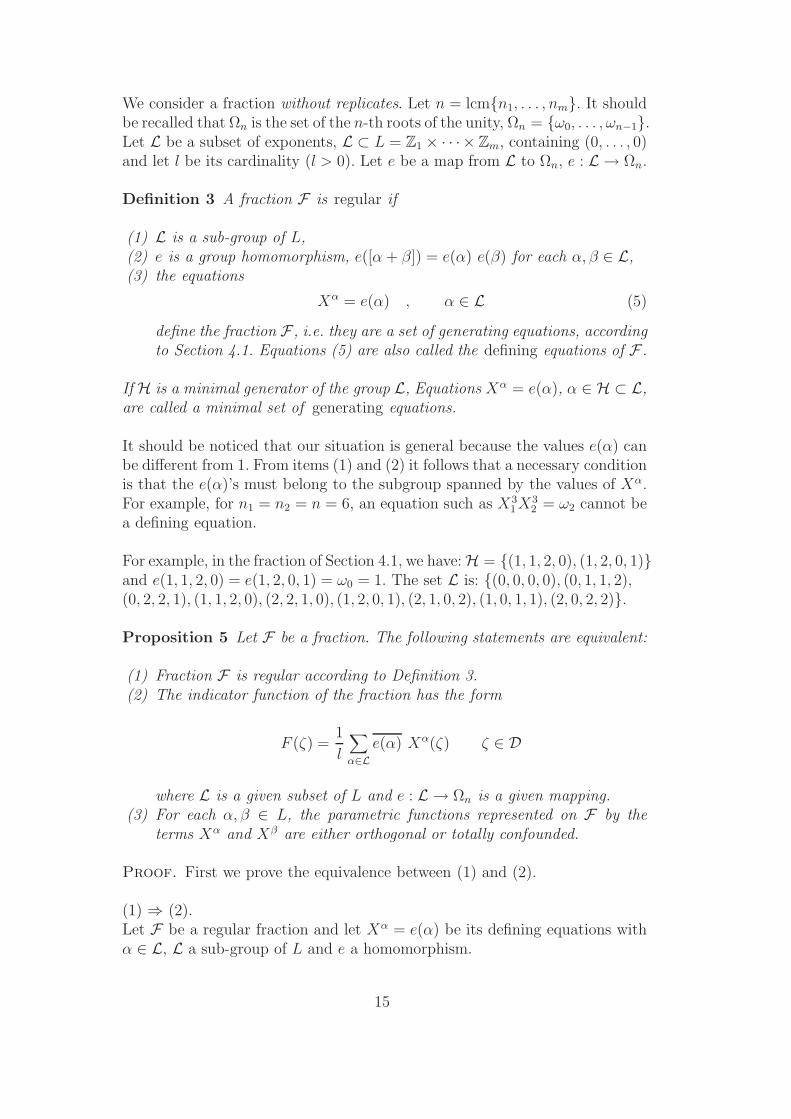
We consider a fraction without replicates. Let n = lcmn1, . . . , nm. It shouldbe recalled that Ωn is the set of the n-th roots of the unity, Ωn = ω0, . . . , ωn−1.Let L be a subset of exponents, L ⊂ L = Z1 × · · · × Zm, containing (0, . . . , 0)and let l be its cardinality (l > 0). Let e be a map from L to Ωn, e : L → Ωn.

Definition 3 A fraction F is regular if

(1) L is a sub-group of L,(2) e is a group homomorphism, e([α + β]) = e(α) e(β) for each α, β ∈ L,(3) the equations

Xα = e(α) , α ∈ L (5)

define the fraction F , i.e. they are a set of generating equations, accordingto Section 4.1. Equations (5) are also called the defining equations of F .

If H is a minimal generator of the group L, Equations Xα = e(α), α ∈ H ⊂ L,are called a minimal set of generating equations.

It should be noticed that our situation is general because the values e(α) canbe different from 1. From items (1) and (2) it follows that a necessary conditionis that the e(α)’s must belong to the subgroup spanned by the values of Xα.For example, for n1 = n2 = n = 6, an equation such as X3

1X32 = ω2 cannot be

a defining equation.

For example, in the fraction of Section 4.1, we have:H = (1, 1, 2, 0), (1, 2, 0, 1)and e(1, 1, 2, 0) = e(1, 2, 0, 1) = ω0 = 1. The set L is: (0, 0, 0, 0), (0, 1, 1, 2),(0, 2, 2, 1), (1, 1, 2, 0), (2, 2, 1, 0), (1, 2, 0, 1), (2, 1, 0, 2), (1, 0, 1, 1), (2, 0, 2, 2).

Proposition 5 Let F be a fraction. The following statements are equivalent:

(1) Fraction F is regular according to Definition 3.(2) The indicator function of the fraction has the form

F (ζ) =1

l

∑

α∈L

e(α) Xα(ζ) ζ ∈ D

where L is a given subset of L and e : L → Ωn is a given mapping.(3) For each α, β ∈ L, the parametric functions represented on F by the

terms Xα and Xβ are either orthogonal or totally confounded.

Proof. First we prove the equivalence between (1) and (2).

(1) ⇒ (2).Let F be a regular fraction and let Xα = e(α) be its defining equations withα ∈ L, L a sub-group of L and e a homomorphism.

15

If, and only if, ζ ∈ F :

0 =∑

α∈L

|Xα(ζ)− e(α)|2 =∑

α∈L

(Xα(ζ)− e(α)) (Xα(ζ)− e(α))

=∑

α∈L

(

Xα(ζ)Xα(ζ) + e(α)e(α)− e(α)Xα(ζ)− e(α)Xα(ζ))

= 2 l −∑

α∈L

e(α)Xα(ζ)−∑

α∈L

e(α) Xα(ζ) = 2

(

l −∑

α∈L

e(α) Xα(ζ)

)

therefore

1

l

∑

α∈L

e(α) Xα(ζ)− 1 = 0 if, and only if, ζ ∈ F .

The function F = 1l

∑

α∈L e(α) Xα is an indicator function, as it can be shownthat F = F 2 on D. In fact, L is a sub-group of L and e is a homomorphism;therefore:

F 2 =1

l2∑

α∈L

∑

β∈L

e(α) e(β) X [α+β] =1

l2∑

α∈L

∑

β∈L

e([α + β]) X [α+β] =

=1

l2∑

γ∈L

l e(γ) Xγ = F.

It follows that F is the indicator function of F , and bα = e(α)l

, for all α ∈ L.

(2) ⇒ (1).It should be noticed that an indicator function is real valued, therefore F = F .

1

l

∑

α∈L

|Xα(ζ)− e(α)|2 = 2− F (ζ)− F (ζ) = 2− 2F (ζ) =

0 on F

2 on D \ F .

Equations Xα = e(α), with α ∈ L, define the fraction F as the generatingequations of a regular fraction. It is easy to see that L is a group. In fact, if γ =[α + β] /∈ L, there exists one ζ such that Xγ(ζ) = Xα(ζ)Xβ(ζ) = e(α)e(β) ⊂Ωn and the value e(α)e(β) only depends on γ. By repeating the previous proof,the uniqueness of the polynomial representation of the indicator function leadsa contradiction.

Now we prove the equivalence between (2) and (3).

(2) ⇒ (3)The non-zero coefficients of the indicator function are of the form bα = e(α)/l.

We consider two terms Xα and Xβ with α, β ∈ L. If [α−β] /∈ L then Xα andXβ are orthogonal on F as the coefficient b[α−β] of the indicator function equals

16

0. If [α−β] ∈ L then Xα and Xβ are confounded because X [α−β] = e([α−β]);therefore Xα = e([α− β]) Xβ.

(3) ⇒ (2).Let L be the set of exponents of the terms confounded with a constant:

L = α ∈ L : Xα = constant = e(α), e(α) ∈ Ωn .

For each α ∈ L, bα = e(α) b0. For each α /∈ L, because of the assumption, Xα

is orthogonal to X0, therefore bα = 0.

Corollary 1 Let F be a regular fraction with Xα = 1 for all the definingequations. F is therefore self-conjugate and a multiplicative subgroup of D.

Proof. It follows from Prop. 2 Item 4.

The following proposition extends a result presented in Fontana et al. (2000)for the two level case.

Proposition 6 Let F be a fraction with indicator function F . We denote theset of the exponents α such that bα

b0= e(α) ∈ Ωn by L . The indicator function

can be written as

F (ζ) = b0

∑

α∈L

e(α) Xα(ζ) +∑

β∈K

bβ Xβ(ζ) ζ ∈ F , L ∩ K = ∅ .

It follows that L is a subgroup and the equations Xα = e(α), with α ∈ L,are the defining equations of the smallest regular fraction Fr containing Frestricted to the factors involved in the L-exponents.

Proof. The coefficients bα, α ∈ L, of the indicator function F are of the formb0e(α). Therefore, from the extremality of n-th roots of the unity, Xα(ζ) =e(α) if ζ ∈ F and Xα(ζ)F (ζ) = e(α)F (ζ) for each ζ ∈ D and L is a group.

We denote the indicator function of Fr by Fr. For each ζ ∈ D we have:

F (ζ)Fr(ζ) =1

lF (ζ)

∑

α∈L

e(α) Xα(ζ) =1

l

∑

α∈L

e(α) Xα(ζ) F (ζ) =

=1

l

∑

α∈L

e(α) e(α) F (ζ) =1

ll F (ζ) .

The relation F (ζ)Fr(ζ) = F (ζ) implies F ⊆ Fr. The fraction Fr is minimalbecause we have collected all the terms confounded with a constant.

17

Remark

Given generating equations Xα1 = 1, . . . , Xαh = 1, with α1, . . . , αh = H ⊂Zn1×· · ·×Znm

, the corresponding fraction F is a subgroup of Ωn1×· · ·×Ωnm

.If the same fraction is represented in the additive notation, such a set oftreatment combinations is the principal block of a single replicate generalizedcyclic design, see John and Dean (1975), Dean and John (1975) and Lewis(1979). A complex vector of the form

(

ei 2π

k1

n1 , ei 2π

k2

n2 , . . . , ei 2π kmnm

)

with 0 ≤ ki < ni, i = 1, . . . , m ,

is in fact a solution of the generating equations if, and only if,

∑mj=1 αij γj kj = 0 mod s

0 ≤ kj < nj

(6)

with s = lcmn1, . . . , nm and γj = snj

.

A set of generators can be computed from Equation (6). It should be noticedthat the following equivalent integer linear programming problem does notinvolve computation mod s, see Schrijver (2002)

∑mj=1 αij γj kj − sq = 0

0 ≤ kj < nj , q ≥ 0(7)

In Lewis (1982), the monomial part of our defining equations is called defin-ing contrast, according to Bailey et al. (1977). The paper contains extensivetables of the generator subgroups of the treatment combinations and the cor-responding defining contrasts.

Viceversa, given a set of generators of the treatment combinations,

b1, . . . , br | bi = (bi1, . . . , bim) ,

Equation (6) with indeterminates αi

∑mj=1 γj bij αj = 0 mod s

0 ≤ αj < nj

produces generating equations for the fraction.

18

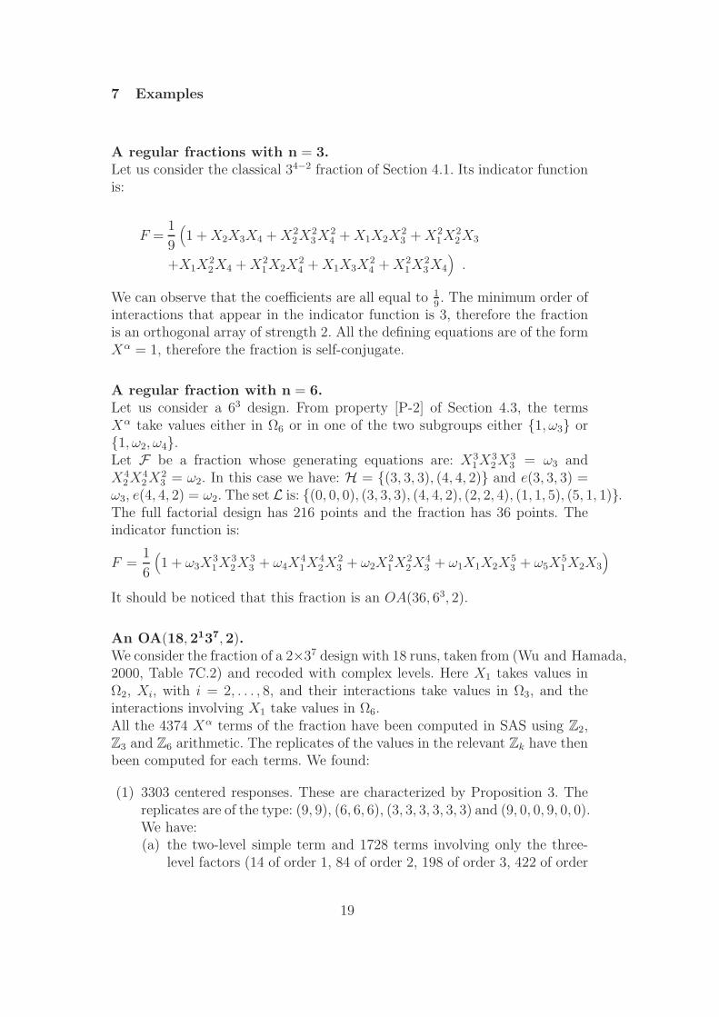
7 Examples

A regular fractions with n = 3.Let us consider the classical 34−2 fraction of Section 4.1. Its indicator functionis:

F =1

9

(

1 + X2X3X4 + X22X

23X2

4 + X1X2X23 + X2

1X22X3

+X1X22X4 + X2

1X2X24 + X1X3X

24 + X2

1X23X4

)

.

We can observe that the coefficients are all equal to 19. The minimum order of

interactions that appear in the indicator function is 3, therefore the fractionis an orthogonal array of strength 2. All the defining equations are of the formXα = 1, therefore the fraction is self-conjugate.

A regular fraction with n = 6.Let us consider a 63 design. From property [P-2] of Section 4.3, the termsXα take values either in Ω6 or in one of the two subgroups either 1, ω3 or1, ω2, ω4.Let F be a fraction whose generating equations are: X3

1X32X3

3 = ω3 andX4

2X42X2

3 = ω2. In this case we have: H = (3, 3, 3), (4, 4, 2) and e(3, 3, 3) =ω3, e(4, 4, 2) = ω2. The set L is: (0, 0, 0), (3, 3, 3), (4, 4, 2), (2, 2, 4), (1, 1, 5), (5, 1, 1).The full factorial design has 216 points and the fraction has 36 points. Theindicator function is:

F =1

6

(

1 + ω3X31X

32X

33 + ω4X

41X

42X

23 + ω2X

21X

22X

43 + ω1X1X2X

53 + ω5X

51X2X3

)

It should be noticed that this fraction is an OA(36, 63, 2).

An OA(18, 2137, 2).We consider the fraction of a 2×37 design with 18 runs, taken from (Wu and Hamada,2000, Table 7C.2) and recoded with complex levels. Here X1 takes values inΩ2, Xi, with i = 2, . . . , 8, and their interactions take values in Ω3, and theinteractions involving X1 take values in Ω6.All the 4374 Xα terms of the fraction have been computed in SAS using Z2,Z3 and Z6 arithmetic. The replicates of the values in the relevant Zk have thenbeen computed for each terms. We found:

(1) 3303 centered responses. These are characterized by Proposition 3. Thereplicates are of the type: (9, 9), (6, 6, 6), (3, 3, 3, 3, 3, 3) and (9, 0, 0, 9, 0, 0).We have:(a) the two-level simple term and 1728 terms involving only the three-

level factors (14 of order 1, 84 of order 2, 198 of order 3, 422 of order

19

4, 564 of order 5, 342 of order 6 and 104 of order 7);(b) 1574 terms involving both the two-level factor and the three-level

factors (14 of order 2, 66 of order 3, 188 of order 4, 398 of order 5,492 of order 6, 324 of order 7 and 92 of order 8).

(2) 9 terms with corresponding bα coefficients equal to b0 = 182×37 = 3−5;

(3) 1062 terms with corresponding coefficients different from zero and b0: 450terms involving only the three-level factors (80 of order 3, 138 of order 4,108 of order 5, 100 of order 6 and 24 of order 7) and 612 terms involvingboth the two-level factor and the three-level factors (18 of order 3, 92 oforder 4, 162 of order 5, 180 of order 6, 124 of order 7 and 36 of order 8).

Some statistical properties of the fraction are:

(1) Analyzing the centered responses we can observe that:(a) All the 15 simple terms are centered.

All the 98 interactions of order 2 (84 involving only the three-levelfactors and 14 also involving the two-level factor) are centered. Thisimplies that both the “linear” terms and the “quadratic” terms of thethree-level factors are mutually orthogonal and they are orthogonalto the two-level factor.The fraction is a mixed orthogonal array of strength 2.

(b) The fraction factorially projects onto the following factor subsets:

X1, X2, X3, X1, X2, X4, X1, X2, X5, X1, X2, X6,

X1, X3, X6, X1, X3, X7, X1, X4, X5, X1, X4, X8,

X1, X5, X8, X1, X6, X7, X1, X6, X8 .

All the terms of order 1, 2 and 3 involving the same set of factors arein fact centered.

(c) The minimal regular fraction containing our fraction restricted to thethree-level factors has the following defining relations:

X22X

24X5 = 1 , X2X4X

25 = 1 ,

X2X3X24X6X7X8 = 1 , X2

2X23X4X

26X

27X

28 = 1 ,

X22X3X

25X6X7X8 = 1 , X2X

23X5X

26X

27X

28 = 1 ,

X3X4X5X6X7X8 = 1 , X23X

24X2

5X26X

27X

28 = 1 .

(d) The non centered terms have levels in Ω6 and in Ω3.

Acknowledgments

We wish to thank many colleagues for their helpful and interesting comments,especially G.-F. Casnati, R. Notari, L. Robbiano, E. Riccomagno, H.P. Wynn

20

and K.Q. Ye. Last but not least, we extensively used the comments and sug-gestions made by the anonymous referees of the previous versions. We regretwe are unable to thank them by name.

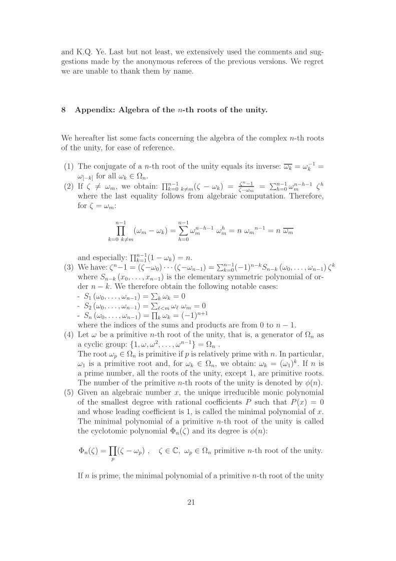
8 Appendix: Algebra of the n-th roots of the unity.

We hereafter list some facts concerning the algebra of the complex n-th rootsof the unity, for ease of reference.

(1) The conjugate of a n-th root of the unity equals its inverse: ωk = ω−1k =

ω[−k] for all ωk ∈ Ωn.

(2) If ζ 6= ωm, we obtain:∏n−1

k=0 k 6=m(ζ − ωk) = ζn−1ζ−ωm

=∑n−1

h=0 ωn−h−1m ζh

where the last equality follows from algebraic computation. Therefore,for ζ = ωm:

n−1∏

k=0 k 6=m

(ωm − ωk) =n−1∑

h=0

ωn−h−1m ωh

m = n ωmn−1 = n ωm

and especially:∏n−1

k=1(1− ωk) = n.(3) We have: ζn−1 = (ζ−ω0) · · · (ζ−ωn−1) =

∑n−1k=0(−1)n−kSn−k (ω0, . . . , ωn−1) ζk

where Sn−k (x0, . . . , xn−1) is the elementary symmetric polynomial of or-der n− k. We therefore obtain the following notable cases:- S1 (ω0, . . . , ωn−1) =

∑

k ωk = 0- S2 (ω0, . . . , ωn−1) =

∑

ℓ<m ωℓ ωm = 0- Sn (ω0, . . . , ωn−1) =

∏

k ωk = (−1)n+1

where the indices of the sums and products are from 0 to n− 1.(4) Let ω be a primitive n-th root of the unity, that is, a generator of Ωn as

a cyclic group: 1, ω, ω2, . . . , ωn−1 = Ωn .The root ωp ∈ Ωn is primitive if p is relatively prime with n. In particular,ω1 is a primitive root and, for ωk ∈ Ωn, we obtain: ωk = (ω1)

k. If n isa prime number, all the roots of the unity, except 1, are primitive roots.The number of the primitive n-th roots of the unity is denoted by φ(n).

(5) Given an algebraic number x, the unique irreducible monic polynomialof the smallest degree with rational coefficients P such that P (x) = 0and whose leading coefficient is 1, is called the minimal polynomial of x.The minimal polynomial of a primitive n-th root of the unity is calledthe cyclotomic polynomial Φn(ζ) and its degree is φ(n):

Φn(ζ) =∏

p

(ζ − ωp) , ζ ∈ C, ωp ∈ Ωn primitive n-th root of the unity.

If n is prime, the minimal polynomial of a primitive n-th root of the unity

21

is Φn(ζ) = ζn−1 + ζn−2 + · · ·+ 1. Moreover:

ζn − 1 = Φn(ζ) · · · ·Φd(ζ) · · · ·Φ1(ζ) where d divides n . (8)

(6) The recoding in Equation (2) is a polynomial function of degree n − 1and complex coefficients in both directions:

ωk =n−1∑

s=0

ωs

∏n−1h=0,h 6=s (x− h)

∏n−1h=0,h 6=s (s− h)

, x = k ∈ 0, . . . , n− 1

k =1

n

n−1∑

h=0

ζhn−1∑

s=1

s ω[s−sh] , ζ = ωk ∈ Ωn . (9)

The last Equation follows from

k =n−1∑

s=1

s

∏n−1h=0,h 6=s (ζ − ωh)

∏n−1h=0,h 6=s (ωs − ωh)

, ζ = ωk ∈ Ωn

and from the properties of the n-th roots of the unity, see Item 2.

References

Bailey, R. A., 1982. The decomposition of treatment degrees of freedom inquantitative factorial experiments. J. R. Statist. Soc., B 44 (1), 63–70.

Bailey, R. A., Gilchrist, F. H. L., Patterson, H. D., 1977. Identification ofeffects and confounding patterns in factorial designs. Biometrika 64, 347–354.

Bose, R. C., 1947. Mathematical theory of the symmetrical factorial designs.Sankhya 8, 107–166.

Cheng, S.-W., Ye, K. Q., 2004. Geometric isomorphism and minimum aberra-tion for factorial designs with quantitative factorss. The Annals of Statistics32 (5).

Collombier, D., 1996. Plans D’Experience Factoriels. Construction et pro-prietes des fractions de plans. No. 21 in Mathematiques et Applications.Springer, Paris.

Dean, A. M., John, J. A., 1975. Single replicate factorial experiments in gen-eralized cyclic designs. II. Asymmetrical arrangements. J. Roy. Statist. Soc.Ser. B 37, 72–76.

Dey, A., Mukerjee, R., 1999. Fractional Factorial Plans. Wiley Series in Prob-ability and Mathematical Statistics. John Wiley & Sons Inc., New York.

Edmondson, R. N., 1994. Fractional factorial designs for factors with a primenumber of quantitative levels. J. R. Statist. Soc., B 56 (4), 611–622.

Fontana, R., Pistone, G., Rogantin, M.-P., 1997. Algebraic analysis and gen-eration of two-levels designs. Statistica Applicata 9 (1), 15–29.

22

Fontana, R., Pistone, G., Rogantin, M. P., 2000. Classification of two-levelfactorial fractions. J. Statist. Plann. Inference 87 (1), 149–172.

Galetto, F., Pistone, G., Rogantin, M. P., 2003. Confounding revisited withcommutative computational algebra. J. Statist. Plann. Inference 117 (2),345–363.

Hedayat, A. S., Sloane, N. J. A., Stufken, J., 1999. Orthogonal arrays. Theoryand applications, With a foreword by C. R. Rao. Springer-Verlag, New York.

John, J. A., Dean, A. M., 1975. Single replicate factorial experiments in gen-eralized cyclic designs. I. Symmetrical arrangements. J. Roy. Statist. Soc.Ser. B 37, 63–71.

Kobilinsky, A., 1990. Complex linear model and cyclic designs. Linear Algebraand its Applications 127, 227–282.

Kobilinsky, A., 1997. Les Plans Factoriels. ASU–SSdF. Editions Technip,Ch. 3, pp. 69–209.

Kobilinsky, A., Monod, H., 1991. Experimental design generated by groupmorphism: An introduction. Scand. J. Statist. 18, 119–134.

Kobilinsky, A., Monod, H., 1995. Juxtaposition of regular factorial designsand the complex linear model. Scand. J. Statist. 22, 223–254.

Lang, S., 1965. Algebra. Addison Wesley, Reading, Mass.Lewis, S. M., 1979. The construction of resolution III fractions from general-

ized cyclic designs. J. Roy. Statist. Soc. Ser. B 41 (3), 352–357.Lewis, S. M., 1982. Generators for asymmetrical factorial experiments. J.

Statist. Plann. Inference 6 (1), 59–64.Pistone, G., Riccomagno, E., Wynn, H. P., 2001. Algebraic Statistics: Compu-

tational Commutative Algebra in Statistics. Chapman&Hall, Boca Raton.Pistone, G., Rogantin, M., 2005. Indicator function and different codings for

fractional factorial designs. Tech. rep., Dipartimento di Matematica, Po-litecnico di Torino.

Pistone, G., Wynn, H. P., 1996. Generalised confounding with Grobner bases.Biometrika 83 (3), 653–666.

Raktoe, B. L., Hedayat, A., Federer, W. T., 1981. Factorial designs. WileySeries in Probability and Mathematical Statistics. John Wiley & Sons Inc.,New York.

Robbiano, L., 1998. Grobner bases and statistics. In: Buchberger, B., Winkler,F. (Eds.), Grobner Bases and Applications (Proc. of the Conf. 33 Years ofGrobner Bases). Vol. 251 of London Mathematical Society Lecture Notes.Cambridge University Press, pp. 179–204.

Robbiano, L., Rogantin, M.-P., 1998. Full factorial designs and distracted frac-tions. In: Buchberger, B., Winkler, F. (Eds.), Grobner Bases and Applica-tions (Proc. of the Conf. 33 Years of Grobner Bases). Vol. 251 of LondonMathematical Society Lecture Notes Series. Cambridge University Press,pp. 473–482.

Schrijver, A., 2002. Theory of linear and integer programming. Wiley-Interscience Series in Discrete Mathematics. Wiley-Interscience [John Wiley& Sons], New York.

23

Tang, B., 2001. Theory of J-characteristics for fractional factorial designs andprojection justification of minimum G2-aberration. Biometrika 88 (2), 401–407.

Tang, B., Deng, L. Y., 1999. Minimum G2-aberration for nonregular fractinalfactorial designs. The Annals of Statistics 27 (6), 1914–1926.

Wu, C. F. J., Hamada, M., 2000. Experiments. John Wiley & Sons Inc., NewYork.

Xu, H., Wu, C. F. J., 2001. Generalized minimum aberration for asymmetricalfractional factorial designs. Ann. Statist. 29 (4), 1066–1077.

Ye, K. Q., 2003. Indicator function and its application in two-level factorialdesigns. The Annals of Statistics 31 (3), 984–994.

Ye, K. Q., 2004. A note on regular fractional factorial designs. Statistica sinica14 (4), 1069–1074.

24