india economic update - world banksiteresources.worldbank.org/indiaextn/resources/... · india...
TRANSCRIPT

December, 2010
Economic Policy and Poverty Team
South Asia Region
The World Bank
India Economic Update

Overview
A Robust Recovery
The Indian economy recovered from the slowdown at the time of the global financial crisis with strong
GDP growth, in particular over the first half of FY2010-11. The agricultural sector bounced back strongly
after the 2010 monsoon brought normal levels of rainfall, and the industrial sector registered double-digit
growth for three consecutive quarters. Inflation came down to 7.5 percent in November but then
accelerated again to 8.4 percent in December because of a renewed food supply shock. The current
account deficit in FY2009-10 was the largest ever (in US$ terms) and the monthly deficit widened further
during the first half of FY2010-11, but the trend then reversed with import growth slowing and export
growth accelerating in September-December 2010. With the significant inflation differential between
India and its trading partners, the rupee‟s real effective exchange rate (REER) strengthened. On the fiscal
side, massive windfall revenue from wireless spectrum auctions and buoyant tax revenue are likely to be
offset by two supplementary spending bills. Monetary policy tightening continued with increases in
policy rates.
Looking forward, GDP growth looks set to regain the pre-crisis trend of around 8.5-9 percent in this year
and the next (FY2011-12). Assuming that the December resurgence in food inflation is temporary, overall
wholesale price inflation is likely to decelerate to 7 percent by end-March 2011 and further during the
coming fiscal year, although uncertainty over international commodity prices persists. The widening trade
deficit during the first half of the year could result in a current account deficit around 3.5 percent of GDP
in FY2010-11, although the recent decline in the trade deficit augurs well for the coming year. Capital
inflows are expected to cover this gap in the current year.
The RBI is likely to continue its policy of cautious rate hikes in a highly uncertain environment. While
inflation has become more broad based, capacity utilization, industrial production, import, and credit
indicators do not point to overheating. The signals are therefore not clear whether core inflation is caused
by more general demand pressures, which would best be addressed with more aggressive policy
tightening, or by second round effects of earlier food and commodity price shocks, for which the current
monetary policy stance is likely to be adequate.
This update also discusses several medium-term issues: the link between the real exchange rate and
growth, a long-term look at education, demographics and growth, the challenges facing the introduction
of the GST, and the mid-term evaluation of the Eleventh Development Plan. On the real exchange rate,
economists have pointed out that the most successful emerging market economies have maintained an
undervalued exchange rate to promote exports. In India, the real exchange rate has been broadly stable
since the early 1990s, and the IMF judges it fairly valued with respect to different measures of
equilibrium. However, the growing trade deficit and a large fiscal deficit do not quite fit this picture.
Discussing policies, we argue that it would be best to focus on policies that increase productivity and
competitiveness.
Education is a strong factor influencing the demographic transition, and it also has direct effects on
economic growth. We present an outlook on India‟s population over the next three decades focusing on
educational attainment. A database for 120 countries allows us to estimate the average relationship
1 Prepared by Ulrich Bartsch, Abhijit Sen Gupta, and Monika Sharma. Helpful comments from Roberto Zagha, Miria Pigato,
Martin Rama, Ivailo Izvorski, Kalpana Kochhar, and Ravi Kanbur are gratefully acknowledged.
India Economic Update1 December, 2010

between education and growth. Applying this to different education scenarios in India highlights the
increase in economic growth that could be expected from a major push for education.
While preparations for the implementation of a Goods and Services Tax are well advanced, political
agreement on the modalities is elusive. The introduction of the GST is intended to broaden the revenue
base and boost growth by removing distortions and increasing integration within India. Discussions are
ongoing about tax rates and which state and local taxes to discontinue, with some of India‟s states fearing
erosion of fiscal autonomy and higher dependence on central transfers.
Lastly, we highlight the Planning Commission‟s Mid-term Assessment of the Eleventh Plan. The most
interesting are its optimism that major goals of the plan, particularly with regard to infrastructure
investment, could be met despite the negative impact of the global financial crisis, and the preview of a
massive step-up in infrastructure spending under the Twelfth Plan.

1
I. Recent Economic Developments
Strong headline GDP growth and quarter-on-
quarter results indicate that the recovery of the
Indian economy is robust. Backed by strong growth
of 8.9 percent y-o-y in the first half of FY2010-11, the
economy is estimated to grow by 8.6 percent during
the fiscal year, as compared with a revised estimate of
8 percent growth for FY2009-10.2 The first and
second quarter growth rates of 8.9 percent were the
highest achieved since Q3 FY2007-08. The quarter-
on-quarter seasonally adjusted annual rate (q-o-q
SAAR) of GDP growth reached 9.0 and 9.3 percent
for the same two quarters.
A low base helped agriculture record a strong
growth rate, but food production is well below
peak levels achieved in earlier years. Agriculture is
expected to grow at 5.4 percent spurred by a low base
in the drought year FY2009-10. The first advance
estimates of kharif (summer) crop production peg
output around 114.6 million tons, a rise of 10.4
percent compared with FY2009-10. The rise in output
was driven by pulses (39.4 percent), jowar (17.2
percent), maize (19.5 percent) and rice (5.9 percent).
However, production in FY2010-11 is estimated to be
well below the levels achieved in FY2007-08 (121
million tons) and FY2008-09 (118 million tons).
The industrial sector registered double digit
growth for three consecutive quarters but slowed
significantly in the October-December quarter. Industrial production (IIP) registered an average
growth of 10.2 percent between April and November
2010. The robust growth was driven by strong
performance of the capital goods and consumer
durables, which grew by 25.8 percent and 22.3 percent
respectively. The manufacturing sector had slowed
down in August and September 2010, but recovered to
register growth of 11.3 percent in October 2010. The
industrial sector is estimated to grow at 8.1 percent in
the fiscal year due to slowing down of the industrial
production in the second half of the year.
On the expenditure side, a resurgence of investment led the recovery, but private consumption
growth is now also picking up. Overall consumption is estimated to grow by 7.3 percent in FY2010-11,
lower than 8.7 percent in FY2009-10. While private consumption growth is set to increase from 7.3 to 8.2
percent, government consumption growth declined from 16.4 percent to 2.6 percent as a result of slowing
2 GDP growth estimate was raised to 8 percent from 7.4 percent for FY2009-10. Advance estimates by CSO for
FY2010-11.
-4.0%-2.0%0.0%2.0%4.0%6.0%8.0%10.0%12.0%14.0%16.0%
-4.0%-2.0%0.0%2.0%4.0%6.0%8.0%
10.0%12.0%14.0%16.0%
07-0
8 Q
1
07-0
8 Q
2
07
-08
Q3
07-0
8 Q
4
08-0
9 Q
1
08
-09
Q2
08-0
9 Q
3
08-0
9 Q
4
09-1
0 Q
1
09
-10
Q2
09-1
0 Q
3
09-1
0 Q
4
10
-11
Q1
10-1
1 Q
2
Agriculture Services GDP Industry
The Rebound in the Agricultural Sector Strengthened.(y-o-y change, in percent)
-4%
-2%
0%
2%
4%
6%
8%
10%
12%
14%
16%
05-
06
Q1
05-
06
Q2
05-
06
Q3
05-
06
Q4
06-
07
Q1
06-
07
Q2
06-
07
Q3
06
-07
Q4
07
-08
Q1
07
-08
Q2
07
-08
Q3
07-
08
Q4
08-
09
Q1
08-
09
Q2
08-
09
Q3
08-
09
Q4
09-
10
Q1
09-
10
Q2
09-
10
Q3
09-
10
Q4
10-
11
Q1
10-
11
Q2
Private Demand Growth Remained Strong. (Components of GDP, y-o-y, change in percent)
GDP Excl. Gov. Cons.
GDP
Source: CSO. Note: Expenditure GDP growth not always same as production.
-20%
-10%
0%
10%
20%
30%
40%
50%
60%
70%
-20%
-10%
0%
10%
20%
30%
40%
50%
60%
70%
05-0
6 Q
105
-06
Q2
05-0
6 Q
30
5-0
6 Q
406
-07
Q1
06-0
7 Q
206
-07
Q3
06-0
7 Q
407
-08
Q1
07-0
8 Q
207
-08
Q3
07-0
8 Q
408
-09
Q1
08-0
9 Q
20
8-0
9 Q
308
-09
Q4
09-1
0 Q
109
-10
Q2
09
-10
Q3
09-1
0 Q
410
-11
Q1
10-1
1 Q
2
Investment Slowed.(Components of GDP, y-o-y change, in percent)
Total Consumption
Private Consumption
Investment
Government Consumption

2
fiscal stimulus spending. Investment (net of stocks) is expected to grow by 8.4 percent in FY 2010-11 as
opposed to 7.3 percent in the previous year.
Food prices renewed their steep climb after a brief slow-down in inflation in the second half of
2010. The WPI inflation rate rose to 8.4 percent in December 2010 from 7.4 percent a month ago,
averaging at 9.4 percent for the period April to December 2010. The recent uptick in inflation can be
attributed to a surge in prices of food articles, which grew by 13.5 percent in December. While food grain
prices have dropped by 2.6 percent in December 2010, the recent surge is due to a spike in fruits and
vegetable prices, which increased by 22.8 percent. Milk, eggs, meat, fish and spices also experienced
double digit inflation rates.
A new wholesale price index was introduced in September 2010 with an updated product basket
and FY2004-05 as base year. While the weights of major product groups have changed little, the new
index has broader coverage (676 items as compared with 435 previously) and nearly three times the
number of price quotations. The new index track the old closely, although the moderation of inflation in
August is more pronounced in the new index than in the old.
The rising merchandise trade deficit pushed the current account deficit to its largest value ever (in
US$ terms). The current account deficit widened to $38.4 billion (2.9 percent of GDP) in FY2009-10.
Nevertheless, strong capital inflows more than compensated for the current account deficit.
Merchandise exports grew by 29.5 percent between
April and December 2010 to reach $164.7 billion.
Over the same period rising oil price and increased
domestic activity pushed imports to $246.7 billion,
increasing by 19 percent from the previous year. The
trade deficit reached US$13bn in August 2010 but has
come down to US$9.5bn in September-October. At the
same time, services exports reacted with a lag to the
global crisis and fell strongly since Q2FY2008-09,
while remittances stabilized. The invisibles‟ surplus
witnessed a slowdown to $79 billion from $90 billion
on account of a deficit in business, financial and
communication services in the first half of FY2010-11.
Capital inflows remained buoyant. Portfolio
investment has been strong for most of the period with
net inflows of $52.6 billion, during April to October
2010. However, November 2010 witnessed a net
outflow of $19.8 billion. There has been a relative
slowdown in FDI flows to $14.0 billion from $19.3
billion during the Apr.-Oct. periods in FY2010-11 and
FY2009-10, respectively. After refraining from
intervention in the foreign exchange market through
most of the first half of FY2010-11, the RBI purchased
$1.3 billion in October and December 2010.
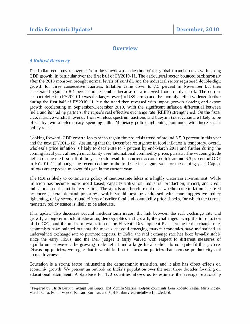
With the significant inflation differential between
India and its trading partners, the rupee’s real
effective exchange rate (REER) strengthened. From
its trough in the wake of the global financial crisis and
-50
-40
-30
-20
-10
0
10
20
1981
-82
1983
-84
1985
-86
1987
-88
1989
-90
1991
-92
1993
-94
1995
-96
1997
-98
1999
-00
2001
-02
2003
-04
2005
-06
2007
-08
2009
-10
The Current Account Deficit Widened(in US$ billion)
60
65
70
75
80
85
90
95
100
105
110
1/20
06
4/20
06
7/20
06
10/2
006
1/20
07
4/20
07
7/20
07
10/2
007
1/20
08
4/20
08
7/20
08
10/2
008
1/20
09
4/20
09
7/20
09
10/2
009
1/20
10
4/20
10
7/20
10
10/2
010
The Real Exchange Rate Appreciated(1993=100)

3
ahead of the May 2009 elections, the REER appreciated
by about 13.6 percent till November 2010 but is still
well below the level it had reached around mid-2007.
Business sentiment is strong, but capacity utilization
is below previous peaks. The RBI‟s industrial outlook
surveys show that companies‟ perceptions of financial
situation and profit margins have recovered to levels
last seen in mid-2007, while selling prices are perceived
to be still lower than at the peak at end-2008. On the
other hand, the RBI‟s Order Books, Inventories and
Capacity Utilization Survey (OBICUS) indicates that
capacity utilization increased during the second quarter
of FY2010-11, but remained below the previous peak.
Capacity utilization in core infrastructure sectors was
largely unchanged from the same period in FY2009-10.
India’s growth resilience and fiscal consolidation
strategy prompted upwards revisions of credit
ratings. Both Moody‟s and Fitch upgraded their local
currency ratings. While Moody‟s upgraded its rating
from Ba2 to Ba1 with a positive outlook, Fitch revised
its rating from negative to stable. These revisions are
likely to encourage FII inflows and strengthening of the
rupee.
Fiscal Developments
Both revenue and expenditure are likely to be higher
than envisaged at the time of the budget. The
government received a massive windfall revenue of
close to Rs.1 trillion (US$20bn, equivalent to 1.8
percent of GDP) from auctions of wireless spectrum.
On the other hand, additional spending was authorized
through adoption by parliament of a first and second
supplementary demand for grants. The supplementary
demands for grants tabled by the government involve an
additional expenditure of Rs.1.1 trillion (1.8 percent of
GDP). A large part of this expenditure, Rs.744 billion
(1.1 percent of GDP) would compensate losses by oil
marketing companies, finance food and fertilizer
subsidy, build roads and houses under centrally
sponsored schemes, and finance transfers to states.
Furthermore, the linking of wages with the CPI would
result in potential higher outgo on NREGA
Tax revenue collections during the first half of
FY2010-11 are promising. Gross tax revenue during
the April-December 2010 stood at Rs.5.28 trillion, up
26.8 percent from the same period last year. Improving
merchandise trade and economic activity as well as reversal of some of the earlier cutbacks in tax rates
resulted in an increase in customs and excise duties of 65.7 percent and 36.5 percent, respectively, over
Oil Under recoveries
19%
PMGSY & Rural Housing
10%
Transfers to State and UTs
8%
Fertilizer Subsidy7%
Food Subsidy
7%Education5%
Rural Development for North East
4%
IMF Quota4%
Defence6%
Police2%
Others28%
Supplementary Spending Bills(Share of total in percent)
-30
-20
-10
0
10
20
30
40
50
3/2
00
5
9/2
00
5
3/2
00
6
9/2
00
6
3/2
00
7
9/2
00
7
3/2
00
8
9/2
00
8
3/2
00
9
9/2
00
9
3/2
01
0
9/2
01
0
3/2
01
1
Industrial Outlook Survey(Perception Indices)
Fin. Situation Selling Prices Profit Margin
Source: RBI
2009-10 2010-11
Finished Steel
(SAIL + VSP + Tata Steel) 87.7 88.9
Cement 80 75
Fertilizer 94.1 94.2
Refinery Production-Petroleum 101.3 102.7
Thermal Power* 72.9 76.2
* Data represent plant load factor for April-December.
Apr.-Oct.
Source: Capsule Report on Infrastructure Sector
Performance (April 2010-October 2010), Ministry of
Statistics and Program Implementation, and Central
Electricity Authority.
Capacity Utilization in Infrastructure Sectors

4
the previous year. Direct tax collection also witnessed
a steady increase with corporate tax revenue
increasing by 20.4 percent and income tax rising by
13.1 percent.
The central government is likely to overperform
on its deficit target under the government’s
accounting rules. However, license fees should be
counted as a financing item because they arose from
the sale of a non-renewable asset much like
privatization revenue. Under this treatment, the
central government deficit is likely to reach 6-6.5
percent of GDP and fiscal consolidation during
FY2010-11 looks feeble.
Monetary Developments
Credit growth and liquidity developments were
largely driven by the result of the telecom
spectrum auctions concluded in June 2010.
Government revenue from auctions of telecoms
licenses was close to Rs.1 trillion. Absorption of
liquidity through payments of the license fee and tax
payments led to a sharp switch in the interbank
market interest rate from the bottom to the top of the
RBI‟s policy rate band (100 basis points between
reverse repo and repo) as banks went from excess
liquidity to liquidity shortage and cash accumulated
in government accounts at the RBI. Broad money expanded by 16.9 percent while reserve money
expanded by 23.6 percent in November 2010 (y-o-y). Credit growth picked up to 18 percent in December
2010 and 20 percent in January 2011, after remaining around 15-16 percent during most of 2010.
Monetary policy tightening continued. With the inflation rate persisting at high levels, the RBI
increased the repo and reverse repo rate in six steps between January 2010 and January 2011 by 150 and
225 basis points, to 6.5 percent and 5.5 percent, respectively.
In a major step to clarify loan pricing, the RBI ruled that commercial banks adopt a Base Rate in
the place of the benchmark prime lending rate (BPLR). The reform is expected to increase the
transparency in lending rates, improve the transmission of monetary policy, and discourage cross-
subsidization of loans. In contrast to the earlier BPLR, banks are now disbarred from lending below the
base rate. It is calculated on the basis of the cost of funds, overhead costs, adjustment for the negative
carry of statutory reserve requirements, and average return on net worth. The banks retain the flexibility
of determining their own lending rates by incorporating customer specific charges as deemed appropriate.
The base rate can be decided on a quarterly basis.
0
5
10
15
20
25
Ap
r-0
5
Jul-
05
Oct
-05
Jan
-06
Ap
r-0
6
Jul-
06
Oct
-06
Jan
-07
Ap
r-0
7
Jul-
07
Oct
-07
Jan
-08
Ap
r-0
8
Jul-
08
Oct
-08
Jan
-09
Ap
r-0
9
Jul-
09
Oct
-09
Jan
-10
Ap
r-1
0
Jul-
10
Oct
-10
Reverse RepoCRRRepoCall Money Rate
Monetary Policy Tightening Continued(Policy Rates and Bombay Interbank Call-Money Rates, in percent)
-1,500
-1,000
-500
0
500
1,000
1,500
2,000
5/3
/20
04
9/3
/20
04
1/3
/20
05
5/3
/20
05
9/3
/20
05
1/3
/20
06
5/3
/20
06
9/3
/20
06
1/3
/20
07
5/3
/20
07
9/3
/20
07
1/3
/20
08
5/3
/20
08
9/3
/20
08
1/3
/20
09
5/3
/20
09
9/3
/20
09
1/3
/20
10
5/3
/20
10
9/3
/20
10
1/3
/20
11
A Liquidity Shortage has Developed(- = injection, in billions of rupees)
Note: RBI Liquidity Adjustment Facility, net bids accepted.Source: RBI.

5
II. Outlook
Global Prospects and Capital Flows
The first half of 2010 witnessed a robust recovery in global GDP growth to 5.25 percent. However,
this benign global picture hides significant heterogeneity among both advanced economies and emerging
markets. Asian economies outside Japan have witnessed rapid growth rates, and the United States has
managed to regain output growth similar to pre-crisis levels, but the output is still well below its pre-crisis
level and unemployment remains uncomfortably large. Germany, on the other hand, has benefited from
an export boom which reduced unemployment to an 18-year low. Despite the German success, the euro
area still contends with an output gap larger than the US‟s. Among the developing countries, both Asian
and Latin American countries have experienced strong growth driven by fixed investment and private
demand. In contrast, developing countries like Mexico, the CIS, and others that had strong trade and
financial linkages with the advanced economies and were therefore more strongly affected by the crisis
are experiencing a more subdued recovery.
Capital Flows to Emerging Markets
(in US$ billions)
2004 2005 2006 2007 2008 2009 2010f 2010f
Private Inflows 426.6 641.7 798.0 1,284.5 594.4 581.4 825.0 833.5
Equity Investment 275.1 359.8 409.9 596.7 422.3 490.4 553.0 549.5
Direct Investment 216.3 288.7 328.6 499.5 508.5 341.8 366.5 406.5
Portfolio Investment 58.8 71.1 81.3 97.2 -86.2 148.7 186.5 143.0
Private Creditors 151.6 281.9 388.1 687.9 172.1 91.0 272.0 283.9
Commercial Banks 65.0 189.2 235.4 451.3 29.1 -44.3 84.9 111.6
Non-banks 86.6 92.7 152.6 236.6 143.0 135.3 187.1 172.3
Source: IIF (2010)
The continuing high unemployment und sluggish growth in most advanced economies has
prevented them from unwinding some of the exceptional liquidity injections undertaken during the
crisis. In fact, the US embarked on a second round of quantitative easing (QE2), thereby again pushing
down yields of US and other securities. While this move was initially expected to lead to a further
significant devaluation of the U.S. dollar, it has so far remained stable against major currencies. Critics
point out, however, that the extra liquidity is likely to exacerbate the surge of capital flows to emerging
economies, which started in the first quarter of 2010. Concerns over exchange rate appreciation, asset
bubbles, and a renewed surge in commodity prices have therefore increased.
Emerging markets are expected to have received
near-record capital inflows. An estimated
US$825billion flowed into emerging economies in
2010, which was nearly 42 percent higher than in 2009
due to relatively high interest rates, strong growth and
improved terms of trade.3 Most of the inflow was in
the form of portfolio equity investments by non-
residents into emerging markets, which rose to
US$186 billion, compared to an annual average of
US$77 billion during 2004 to 2007. In contrast,
commercial bank inflows are estimated to be
3 See IIF (2010).
0
200
400
600
800
1000
Jan
-09
Mar-
09
May-0
9
Ju
l-09
Se
p-0
9
No
v-0
9
Jan
-10
Mar-
10
May-1
0
Ju
l-10
Se
p-1
0
No
v-1
0
Sovereign Bond Interest Spreads
BRACHNIDNMYSPHL
6
significantly lower at US$84.9 billion as opposed to an
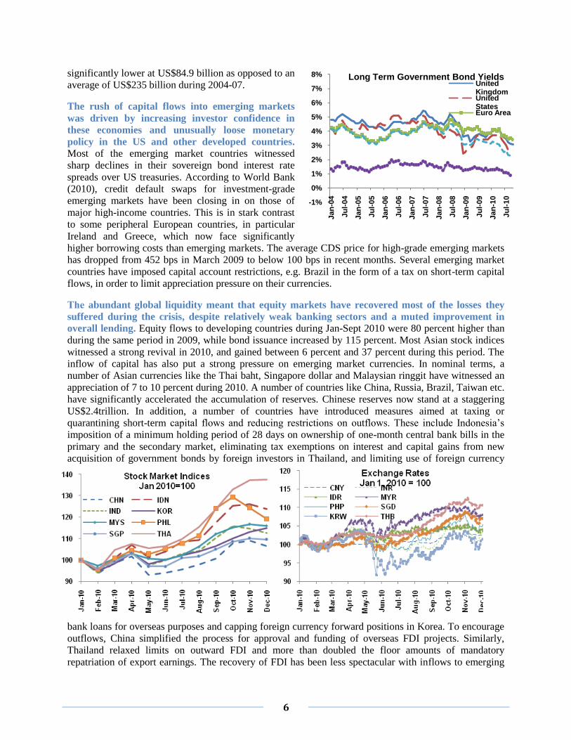
average of US$235 billion during 2004-07.
The rush of capital flows into emerging markets
was driven by increasing investor confidence in
these economies and unusually loose monetary
policy in the US and other developed countries. Most of the emerging market countries witnessed
sharp declines in their sovereign bond interest rate
spreads over US treasuries. According to World Bank
(2010), credit default swaps for investment-grade
emerging markets have been closing in on those of
major high-income countries. This is in stark contrast
to some peripheral European countries, in particular
Ireland and Greece, which now face significantly
higher borrowing costs than emerging markets. The average CDS price for high-grade emerging markets
has dropped from 452 bps in March 2009 to below 100 bps in recent months. Several emerging market
countries have imposed capital account restrictions, e.g. Brazil in the form of a tax on short-term capital
flows, in order to limit appreciation pressure on their currencies.
The abundant global liquidity meant that equity markets have recovered most of the losses they
suffered during the crisis, despite relatively weak banking sectors and a muted improvement in
overall lending. Equity flows to developing countries during Jan-Sept 2010 were 80 percent higher than
during the same period in 2009, while bond issuance increased by 115 percent. Most Asian stock indices
witnessed a strong revival in 2010, and gained between 6 percent and 37 percent during this period. The
inflow of capital has also put a strong pressure on emerging market currencies. In nominal terms, a
number of Asian currencies like the Thai baht, Singapore dollar and Malaysian ringgit have witnessed an
appreciation of 7 to 10 percent during 2010. A number of countries like China, Russia, Brazil, Taiwan etc.
have significantly accelerated the accumulation of reserves. Chinese reserves now stand at a staggering
US$2.4trillion. In addition, a number of countries have introduced measures aimed at taxing or
quarantining short-term capital flows and reducing restrictions on outflows. These include Indonesia‟s
imposition of a minimum holding period of 28 days on ownership of one-month central bank bills in the
primary and the secondary market, eliminating tax exemptions on interest and capital gains from new
acquisition of government bonds by foreign investors in Thailand, and limiting use of foreign currency
bank loans for overseas purposes and capping foreign currency forward positions in Korea. To encourage
outflows, China simplified the process for approval and funding of overseas FDI projects. Similarly,
Thailand relaxed limits on outward FDI and more than doubled the floor amounts of mandatory
repatriation of export earnings. The recovery of FDI has been less spectacular with inflows to emerging
-1%
0%
1%
2%
3%
4%
5%
6%
7%
8%
Jan
-04
Ju
l-04
Jan
-05
Ju
l-05
Jan
-06
Ju
l-06
Jan
-07
Ju
l-07
Jan
-08
Ju
l-08
Jan
-09
Ju
l-09
Jan
-10
Ju
l-10
Long Term Government Bond YieldsUnited KingdomUnited StatesEuro Area

7
markets expected to have increased by only 7.2 percent in 2010, compared to a decline of 32 percent in
2009. Much of this rise in FDI is due to an increase in South-South FDI, with the BRIC countries
accounting for 60 percent.
Is India Making Development more Sustainable
through Effective Enforcement of Environmental Compliance?
The challenge of environmental management and regulation is immense, but India has a credible
legislative and policy base to foster environmental sustainability. However, gaps are evident in the
institutional mechanisms for enforcement and compliance, as well as the implementation and
mainstreaming of environmental issues across various sectors of the economy. During recent years, the
Ministry of Environment and Forest (MoEF) has clearly raised the profile of environmental concerns
and inclusive growth in the Government of India‟s development agenda, and Prime Minister Singh
pointed out that disregard of environmental and social issues would lead to “perpetuating poverty”.1
Four recent decisions by the MoEF have made headlines: the cancellation of the “in principle”
environmental clearance provided two years ago to an alumina refinery in Orissa‟s Kalahandi District
and a Bauxite mine in the Niyamgiri Hills, the scrapping of three hydro-electric projects in the
Bhagirathi basin, the withholding of environmental clearance to any other of the hydro-electric projects
planned in the Bhagirathi and Alaknanda basins (tributaries of the Ganges) till the completion of
cumulative impact analyses for the basins, and the stay order on construction of the new city Lavasa in
Maharashtra. There have been determined efforts to bring greater transparency and professionalism to
the granting of environmental and forestry clearances, further facilitated through the Right to
Information Act. New initiatives also aim at addressing institutional and compliance gaps: a National
Environmental Protection Agency (NEPA) will focus on enforcement and monitoring of
environmental laws in the country, and „Green Tribunals„ will rule on environmental disputes of a civil
nature including the provision of compensation for damage to persons and property.
Major boosts to the sustainable development agenda are also expected from linking central grants to
India‟s states to environmental performance. A „Green Index‟ to be developed by the Planning
Commission based on a review of the air and water quality, forest cover, size of national parks, and
climate change gas emissions will rule over the disbursement of around Rs.19 billion (US$400 million)
to the states in FY2010-11.1
The recent legal actions and responses from communities and NGOs are a clear indication that
sustainable development of infrastructure rests on transparency and meaningful participation of all
stakeholders, especially the marginalized sections of society affected by the project. At the same time,
effective implementation and enforcement of the regulatory framework and its underlying provisions is
required to ensure that environmental and social issues do not become a constraint to economic
development.
Contributors: Pyush Dogra and Sonia Chand Sandhu

8
India Outlook
Strong growth is likely to be sustained. GDP growth
for FY2010-11 and FY2011-12 is likely to reach 8.5-9
percent. The high growth of the two last quarters (Q1
and Q2 of FY2010-11) surprised analysts. In
particular, the strong Q2 growth came on the back of a
relatively strong performance in the same period a year
earlier and therefore did not benefit from a positive
„base effect‟. However, growth would still partially be
a rebound from the slowdown in the wake of the global
financial crisis, and could therefore appear somewhat
weaker in subsequent quarters. Slower IIP growth and a
slowdown in imports points into the same direction.
The current account deficit is likely to widen
significantly from the record deficit of FY2009-10.
Initially, imports recovered more strongly than exports
from the slowdown and the “great trade collapse”
during the global financial crisis. Growing services
surpluses and net transfers have compensated for rising
trade deficits in the past. However, the picture now
looks less benign. Extrapolating from the trends in
merchandise trade, services and transfers, the
remainder of the current fiscal year would produce a
current account deficit of around US$40 billion for
FY2010-11, an increase from the record deficit
recorded in FY2009-10.
Capital inflows are expected to continue to be strong
and pose risks in both directions. While FDI held up
well during the global crisis, recent numbers have
disappointed. Portfolio investments are likely to
continue at levels similar to those observed recently,
although volatility could be high. Loans have recovered
strongly and now constitute the biggest item in the
capital account. At current levels of inflows, the capital
account surplus would be sufficient to cover the current
account gap. However, renewed shocks to the global
financial system could quickly change investor
perceptions and lead to another “flight to safety”. The
risk for such shocks occurring is high in light of the
unsettled debt issues in some European countries. On
the other hand, global liquidity remains unusually high
with little prospects for monetary policy tightening in
major developed countries in 2011. High liquidity
could lead to sudden FII surges in emerging markets.
The RBI has demonstrated its ability to react quickly to
short-term capital flows and its reserves remain
sufficient to prevent unwanted volatility of the rupee.
-20.0
-16.0
-12.0
-8.0
-4.0
0.0
4.0
8.0
12.0
16.0
20.0
-20.0
-16.0
-12.0
-8.0
-4.0
0.0
4.0
8.0
12.0
16.0
20.0
20
05
Q4
20
06
Q3
20
07
Q2
200
8Q
1
20
08
Q4
20
09
Q3
201
0Q
2
20
11
Q1
20
11
Q4
20
12
Q3
201
3Q
2
20
14
Q1
20
14
Q4
20
15
Q3
Macroeconomic Indicators
Actual CY2006-10Q2, Forecast CY2010Q2-15
(in %)
Output Gap Y-o-y Inflation Real Interest Rate
Nom. Int. Rate Exchange Rate Gap
Forecast
0.00
5,000.00
10,000.00
15,000.00
20,000.00
25,000.00
30,000.00
35,000.00
40,000.00
45,000.00
Sep
-03
Mar
-04
Sep
-04
Mar
-05
Sep
-05
Mar
-06
Sep
-06
Mar
-07
Sep
-07
Mar
-08
Sep
-08
Mar
-09
Sep
-09
Mar
-10
Sep
-10
Mar
-11
The Current Account Deficit Could Fall Further.(in US$ million)
Merchandise Trade Balance (-)
Services Balance
Net Transfers
Proj.
-10,000.00
-5,000.00
0.00
5,000.00
10,000.00
15,000.00
20,000.00
25,000.00
Sep
-03
Dec
-03
Mar
-04
Jun
-04
Sep
-04
Dec
-04
Mar
-05
Jun
-05
Sep
-05
Dec
-05
Mar
-06
Jun
-06
Sep
-06
Dec
-06
Mar
-07
Jun
-07
Sep
-07
Dec
-07
Mar
-08
Jun
-08
Sep
-08
Dec
-08
Mar
-09
Jun
-09
Sep
-09
Dec
-09
Mar
-10
Jun
-10
Sep
-10
Dec
-10
Mar
-11
Capital Inflows Remained Robust(in US$ millions)
FDI FII Loans
Proj.
Sources: RBI, WB, and author's calculations.
0
5000
10000
15000
20000
25000
30000
35000
Jan
-00
Au
g-00
Mar
-01
Oct
-01
May
-02
Dec
-02
Jul-
03
Feb
-04
Sep
-04
Ap
r-0
5
No
v-05
Jun
-06
Jan
-07
Au
g-07
Mar
-08
Oct
-08
May
-09
Dec
-09
Jul-
10
Feb
-11
Sep
-11
Imports
Exports
Imports and Exports, actual to December 2010, forecasts to October 2011(in US$ millions)
Note: Seasonally adjusted.
Proj.

9
The current and capital account movements make the direction of the rupee hard to forecast. When
the current account deficit was high in the first three quarters of 2010, capital inflows were strong. When
the current account deficit narrowed during the last quarter of the year, portfolio flows reversed. The
result was a relatively stable rupee during much of the year. In the near term, this stability is likely to
hold, while towards the second half of 2011 appreciation pressure is likely to return. Because of the
inflation differential between India and its trading partners, the real effective exchange rate is projected to
appreciate further.
Monetary policy is walking a tightrope between supporting growth and fighting inflation. The RBI
is likely to continue tightening its policy rates in the first two quarters of 2011, although rate increases are
likely to be limited. Real interest rates are currently below historical averages, but falling inflation and
further rate hikes would allow them to normalize in the next few months. With progress in disinflation,
policy rates should peak in the second half of FY2011-12 and then fall, in line with falling inflation. The
environment for monetary policy decisions is highly uncertain. Food inflation is expected to moderate
(see next section) and monetary policy instruments are in any case ill suited to address it. External and
temporary supply shocks are best accommodated, i.e. the central bank should raise rates to prevent real
interest rates from falling but should not raise them aggressively. RBI‟s recent step-wise, cautious rate
hikes seem to have followed this concept. Apart from the inflation indices, other signals about the demand
and supply balance in the Indian economy are mixed: capacity utilization indicators are stable, while the
recent industrial production and imports data point to a slowdown rather than overheating. On the other
hand, credit growth has picked up in December 2010 and January 2011, although it can hardly be seen as
excessive. The signals are therefore mixed as to whether inflation is caused by more general demand
pressures, which would call for more aggressive monetary policy tightening, or by second round effects
of earlier food and commodity price shocks, for which the current policy stance would be adequate.
A Look at Inflation
Global commodity prices have started to rise after a period of some stability in the wake of the
global financial crisis. The last months of 2010 saw a pronounced increase in international prices, in
particular those of food commodities. The increase in U.S. dollar prices is moderated somewhat by the
U.S. dollar depreciation against major currencies, but the trajectory is worrying. Rice prices retreated to
about twice their historic levels from the peak of 3.5 times and have fallen again since March 2010.
Wheat prices declined through June 2010, but have since shot up by more than 60 percent. The supply
and demand balance cannot entirely explain the sudden rise. Disruptions in Russia reduced wheat
production there by 40 percent, but global production is only about 5 percent below last year‟s. This still
leaves it 8 percent higher than in 2008. On the other hand, oil prices recovered to around US$75 per
barrel in early 2009 and have since inched up to $90 per barrel in December 2010. The real price index on
the other hand is fairly stable since October 2009.
While the supply and demand balance does not
present cause for worries, global liquidity remains
exceptionally high, and interest rates in major
economies low – two factors that could contribute
to a renewed speculative commodity price rally.
India’s inflation trajectory is similar to that of
other emerging markets, but India’s level of
inflation is relatively high. Inflation accelerated in
the run-up to the global financial crises, dropped
into negative territory as global commodity prices
collapsed during the crisis, and accelerated again in
early-mid-2010. India‟s inflation was comparable to
-15.0
-10.0
-5.0
0.0
5.0
10.0
15.0
20.0
25.0
M1
20
06
M3
20
06
M5
20
06
M7
20
06
M9
20
06
M1
1 2
00
6
M1
20
07
M3
20
07
M5
20
07
M7
20
07
M9
20
07
M1
1 2
00
7
M1
20
08
M3
20
08
M5
20
08
M7
20
08
M9
20
08
M1
1 2
00
8
M1
20
09
M3
20
09
M5
20
09
M7
20
09
M9
20
09
M1
1 2
00
9
M1
20
10
M3
20
10
M5
20
10
M7
20
10
M9
20
10
M1
1 2
01
0WPI Inflation in Major Emerging Market Economies
(y-o-y change in percent)
India Brazil China Thailand Philippines Malaysia Korea

10
that of major Asian EMEs and Brazil in the 2008 rally, dropped less than the mean during the global
crisis, and recovered to somewhat above the mean in 2010. In the chart, Thai inflation is higher than
Indian except in the very end of the year when Brazilian inflation overtakes both. In the group shown
except in Brazil, inflation seems to have passed a peak and dropped in recent months, which is partly a
result of the fading base effect of low prices in 2009.
In India, food inflation is remaining stubbornly high, while core inflation is now also high. Core
inflation is driven by second-round effects of the food price pressure, high commodity prices, and
possibly rising capacity utilization. Core inflation
(non-food, non-fuel) began to accelerate in the early
months of 2010 and reached 8.5 percent in
November 2010, but fell back to 7.5 percent in
January 2011. Support for the argument that this
reflects to some extent second-round effect of the
food price shocks comes from data collected for the
CPI on personal services. These show a significant
increase in non-tradable prices and wages. Higher
core inflation has been cited by the RBI as a
worrying sign that inflation is becoming entrenched.
In fact, long-term inflationary expectations in the
RBI‟s survey data recently shifted upward by 0.5
percentage points. A renewed increase in
international food and energy commodity prices
could also lead to a renewed price spiral in India, similar to what was observed in FY2007-08. Current
projections of the global demand and supply balances for commodities do not point to another price
boom, but the outlook is highly uncertain. WPI inflation is projected to fall to around 7 percent by end-
March 2011, and 4-5 percent by the end of FY2011-12.
A near-normal monsoon should put downward pressure on food prices in India. The monsoon in
India is important, not only for the largely rain-fed kharif (summer) crop, but also for replenishing
reservoirs for the irrigated rabi (winter) crop. The near-normal summer 2010 monsoon is expected to lead
to further easing of price pressures on primary food articles with the upcoming winter harvest, although
transportation disruptions and local flooding led to some renewed price pressures in late August-early
September 2010 and again in November 2010. Production of rice, wheat and pulses is expected to
increase significantly over last year. Wheat production is projected to be 80.7 million metric tons (mt)
while consumption is projected to be 82.4 million mt (USDA). Rice production is projected to increase to
99.0 million mt with consumption projected to be around 98.0 million mt.
The government’s handling of food grain has come under increased pressure. The Food Corporation
of India (FCI) buys food grains from India‟s farmers at prices set by the government (Minimum Support
Prices, MSP) to hold precautionary stocks and release grains to stores to be sold at subsidized prices to
poor households (the public distribution system, PDS). Buffer stocks of wheat and rice held by the FCI
reached 50 million Mt in July as against the norm of 27 million Mt. The simultaneous occurrence of high
food inflation and large food-grain stocks has become a matter of widespread concern.
-15
-10
-5
0
5
10
15
20
25
-15
-10
-5
0
5
10
15
20
25
Jan
-08
Ap
r-0
8
Jul-
08
Oct
-08
Jan
-09
Ap
r-0
9
Jul-
09
Oct
-09
Jan
-10
Ap
r-1
0
Jul-
10
Oct
-10
Jan
-11
Ap
r-1
1
WPI-AllWPI- CoreWPI - FoodWPI- Energy
Indian Food Inflation is Lingering, Overall Inflation Will Fall Very Slowly...(Components of WPI, y-o-y change, in percent)
Note: Extrapolation of average of past 6 monthly increases.Sources: CSO and authors' calculations.
Forecast

11
III. Real Exchange Rate and Growth
Developments in the exchange rate are at the heart of discussions of economic policies in India
because of the increasing openness of the economy to current and capital account transactions. The
rupee has shown considerable volatility in the last two years – first appreciating strongly against the U.S.
dollar on the back of massive foreign capital inflows in late 2007 – early 2008, then depreciating by more
than 20 percent during the global financial crisis, and now appreciating again since May 2009. There is
therefore a concern that appreciation of the rupee against the U.S. dollar would be detrimental for exports
which, in turn, would be detrimental for growth. This section discusses the rationale and empirical
evidence regarding the link between the exchange rate, exports, and long-run economic growth, as well as
policy implications. This is necessarily a very short summary of a complex subject.
A Perspective on Rising Minimum Support Prices (MSP)
A recent paper studies the relationship between cost of production (CoP), support prices, prices realized and
wholesale prices.1 It argues that the shift in agricultural policy since the 1990s emphasized price intervention over
non-price interventions, which resulted in a decline in the growth rate of yields and a rise in the costs of production.
Support prices were raised repeatedly to sustain the long-run margin over total costs.
Years Rice Wheat
CoP MSP
MSP over
cost (%) CoP MSP
MSP over
cost (%)
2005-06 557.6 600 7.6 541.5 700 29.3
2006-07 569.5 650 14.1 573.6 850 48.2
2007-08 595 775 30.3 624.5 1000 60.1
2008-09 619 930 50.2 648.6 1080 66.5
2009-10 644.9 1030 59.7 741.0 1100 48.4 Note: Cost of production includes transportation, insurance premium and marketing charges.
The MSPs declined in the 1980s in real terms but returns to farming remained adequate because costs of production
fell during the period as productivity improved at more than 2.5 percent per annum. On the other hand, the costs of
production rose at the rate of nearly 1.5 percent per annum in both crops during the 1990s and beyond as yield
growth slowed. MSPs were raised to help farmers maintain their incomes. The authors blame the slowdown in yield
growth on dwindling non-price interventions such as public investments. The second major factor driving higher
support prices is the operation of market forces in a liberal and open trade regime. When the international market
prices are higher and rising as a result of a supply shock, domestic prices of the respective commodity shoot up and
procurement of sufficient quantities to the required levels to ensure food security becomes difficult. Therefore, the
government will have to offer higher prices, as happened in 2007 and 2008 in the case of wheat, making the gross
margin more than 50 percent. The pulls and pressures of democracy and farmer lobbies make it impossible to roll
back these prices, even if global prices recede considerably.
A related influential paper proposes an overhaul of the entire system of government intervention in food production,
procurement and distribution by the FCI.2 In particular, a new set of rules would be needed on when and how to
release food grains from the public stocks to stabilize prices. With the current policy, releasing stocks is hampered
by an attempt to sell grain at prices higher than the procurement prices, which results in low or no off-take when
prices are above market, and stringent controls are imposed on buyers. Grain released through open market
operations by the FCI is sold to millers in bulk, and only rarely to traders. The millers are then prohibited from
onward selling to traders. It is not clear why grain cannot be released in small quantities to large numbers of traders
and millers to allow competition between them to keep prices low.
1 Dev and Rao (2010).
2 Basu (2010).

12
Export-led growth strategies have been credited with the resounding success of several economies,
especially in East Asia in achieving rapid improvements in living standards. In fact, studies show that
nearly all developing countries that experience sustained growth also show an increase in the share of
manufacturing exports in GDP.4 Some economists propose that the production of tradables provides
greater opportunities for productivity increases than the production of non-tradables. Some of the
dynamic effects of tradables are thought to be externalities – learning by doing, investment in search for
opportunities which are then available to everyone – and a market-based equilibrium would leave
production below the social optimum. Another argument is that the size of the domestic market in poorer
countries is not sufficient to provide the employment opportunities needed to absorb the surplus labor.
There are indications that at least some of the fast-growing countries relied, and still rely, on measures
aimed at undervaluing the real exchange rate to reduce the consumption of tradables but improve the
profitability of their production for exports.5 Undervaluation means that non-tradables are somehow made
cheaper relative to tradables than what they would be without policy intervention, which allows
consumption to switch to non-tradables while the production of tradables for export receives a boost.6
Some cross-country studies support the view that the level of the real exchange rate is correlated
with economic growth but the direction of causality is hotly debated.7 It is very difficult to
disentangle the direct effects on growth of policies that also move the real exchange rate from the effects
on growth of the exchange rate itself. For example, the policies that lead to and maintain overvaluation –
rationing of foreign exchange, foreign exchange controls – have direct effects on investment in the
tradables sector, which are possibly more damaging than the loss of competitiveness of the tradables
sector from overvaluation. Those who see a causal link between undervaluation and growth argue that
undervaluation is needed because (potential) producers of tradables suffer disproportionately from the
institutional weaknesses and market failures that characterize low-income countries. Undervaluation is
akin to a blanket subsidy aimed at helping tradables to overcome these barriers. Critics argue that the
studies used to support the undervaluation-high growth causal chain suffer from omitted variables. For
example, an increase in domestic savings and investment simultaneously depreciates the real exchange
rate and boosts growth.8
The evidence for the existence of externalities and spillovers from exports is mixed. There are several
studies which support the thesis that increasing the share of manufacturing exports is good for growth.9
The evidence on positive spillovers from exporting, however, is less than conclusive. A number of studies
report that proximity to other exporting firms increases the likelihood that a subject firm will itself
4 Johnson, Ostry and Subramaniam (2007). 5 See for example Krueger, A.O. (1998). Real exchange rate undervaluation was not the only enabling factor: abundant cheap
labor, subsidized credit, energy, infrastructure, supportive tax and tariff rates are also described in the literature. 6 Non-tradables in low-income countries are necessarily cheaper than in high-income countries, and real exchange rates therefore
appreciate when countries grow richer – so so-called Balassa-Samuelson effect. The focus here is on lowering the relative price
of non-tradables beyond what the market would produce. 7 Rodrik (2008) and Haddad and Pancaro (2010). The latter shows that the effect seems to fade over time and may actually
reverse – i.e., undervaluation may be detrimental to growth in the long run. Real exchange-rate volatility is detrimental to growth
and the difficulties in maintaining real exchange-rate undervaluation over time may lead to volatility which could explain the
long-run reversal of its effects on growth. Eichengreen (2008) is another proponent, while Woodford (2009) provides a strong
critique of Rodrik‟s methodology and argumentation. 8 Bernanke (2005) argues that while a relationship between depreciated real exchange rate and high savings rate exists the
causality goes from a depreciated real exchange rate to a high saving rate to a high growth rate driven by capital accumulation.
Montiel and Serven (2008) find that exchange rate policy in general, or a depreciated real exchange rate has not been identified as
an important factor in explaining differences in savings rate. Even in the high saving, high-growth countries key determinants of
saving rates have been identified as demographics, financial sector policies, mandated saving schemes, and fiscal policies, rather
than exchange rate policies. 9 Jones and Olken (2005) find significant reallocation of resources toward manufacturing during growth upturns. Johnson et al.
(2007) find that nearly all developing countries that experience sustained growth also witness a rapid increase in their shares of
manufacturing exports. Similarly, Rodrik (2006) argues that rapidly growing developing countries tend to have unusually large
manufacturing sectors and that growth accelerations are associated with structural shifts in the direction of manufacturing.

13
export.10
However, there are other studies showing that the tendency of firms to export is not affected by
their proximity to other exporters.11
Fairly robust evidence shows that there is indeed a productivity
differential between exporters and domestic firms.12
However, there do not seem to be any learning-by-
doing effects from exporting. Rather, firms self-select into exports, i.e. they go into export markets after
they have somehow managed to establish a productivity premium. The empirical evidence therefore does
not show greater dynamism for improving TFP in exports relative to home production.
India’s Exchange Rate Management
Nominal and real exchange rate indices show that
India maintained a fair degree of stability
throughout the liberalization period after 1991. The nominal effective exchange rate depreciated by
about 10 percent in the early 1990s and stabilized
thereafter, until it experienced a pronounced
appreciation during the capital inflow boom in 2007.
The real effective exchange rate, calculated by RBI
on the basis of trade weights, also showed a
depreciating trend in the 1990s, but returned to the
1993 level in the 2000s. Exchange rate volatility
increased markedly from 2007 as the RBI intervened
less in foreign exchange markets. The capital inflow
boom brought appreciation in 2007, which was followed by a significant depreciation in the wake of the
global financial crisis. In the aftermath of the crisis, both the nominal and the real exchange rate bounced
back strongly but in October 2010, the real exchange rate index reached 99.7, which was well below the
peak it had reached in 2007.
While it is common to observe the rate of change of the real exchange rate, indirect methods are
needed to evaluate its level. Economists compare the developments of domestic and foreign prices
(converted at market exchange rates).13
The resulting index numbers give an indication of the change in
the real exchange rate over time, but they do not in themselves enable us to judge whether the real
exchange rate is over- or undervalued. A methodology used to judge the level of the real exchange rate
rather than its direction of change involves estimating whether or not the economy is in external and
internal equilibrium. This Equilibrium Method is used by the IMF‟s Consultative Group on Exchange
Rate issues (CGER).14
The IMF judges the Indian rupee to be fairly valued relative to different concepts
of medium-term equilibrium. Another method compares market exchange rates with purchasing power
parity exchange rates (the PPP method used by Rodrik and others). The difficulty in using this
methodology is to make an appropriate adjustment for the fact that the relative price of non-tradable
goods is higher in countries with higher income per capita (the Balassa-Samuelson effect).15
10 Lin (2004) finds that the propensity for Taiwanese firms to export is positively affected by the propensity to export of other
firms in the same industry in its geographic vicinity. Koenig (2005) reports similar results for a sample of French firms, while
Alvarez and Lopez (2006) report evidence of horizontal productivity spillovers from exporting for a sample of Chilean firms. 11 Aitken et al. (1997), Barrios et al. (2003), Bernard and Jensen (2004), and Lawless (2005). 12 International Study Group on Exports and Productivity (2008). 13
The rationale is that tradable prices are determined in the international market while non-tradable prices are determined in the
domestic market. Comparing price indices between two or more countries therefore is a proxy for the real exchange rate as long
as the „law of one price‟ holds, i.e. tradables cost the same (adjusted for transport and other costs) in different countries. 14
IMF (2006). 15 The undervaluation index (UNDERVAL) is computed as the residual of a regression of the real exchange rate (RER) on real
GDP per capita (RGDPCH), where RERit is defined as the ratio between the nominal exchange rate (XRAT) and the purchasing
6065707580859095
100105110
Ap
r-9
3
Jul-
94
Oct
-95
Jan
-97
Ap
r-9
8
Jul-
99
Oct
-00
Jan
-02
Ap
r-0
3
Jul-
04
Oct
-05
Jan
-07
Ap
r-0
8
Jul-
09
Oct
-10
REER
NEER
Real and Nominal Exchange Rate Indices(1993=100)

14
India’s current account and fiscal deficits are not pointing to undervaluation of the exchange rate. India has never been able to achieve a trade surplus and the current account has recorded a deficit during
most years post independence. The current account deficit hovered around 2 percent of GDP during much
of the 1970s and 1980s, and improved after the balance of payments crisis in 1991 to reach a brief surplus
of 2 percent in 2003. Since then, the current account has deteriorated again to probably reach a deficit of
3.5 percent of GDP in FY2010-11. Large inflows of remittances mask the widening trade deficit,
especially in recent years. More recently, imports actually grew faster than exports. The trade deficit
reached a record 6 percent of GDP in FY2008-09 and narrowed a little in FY2009-10, but is again
widening in FY2010-11. In fact, trade made a negative contribution to growth in a national accounting
sense in most years of the 2000s. India‟s government accounts were also in deficit over recent decades, a
situation usually associated with exchange rate overvaluation. In fact, India‟s fast growth, particularly in
the 2000s, seems to have been fueled by a growing domestic market with imports of capital and consumer
goods financed to a large degree by remittances and foreign savings.
India’s Trade and Domestic Production
India may differ from other emerging markets because of its size. If the domestic market is
sufficiently attractive, domestic entrepreneurs and foreign investors set up sophisticated production
capacity for the domestic market, rather than for export. They compete with imported products, thereby
importing skills and technologies. The car industry is an interesting example of capacity being created to
compete with imports, and learning-by-doing improvements in productivity that eventually produce an
exportable surplus.
There is–admittedly weak–evidence that home production in India is as ‘sophisticated’ as exports. This result is obtained by comparing the share of
„sophisticated‟ goods in exports, as shown in UN trade
statistics, with their share in domestic production, as
shown in India‟s Annual Survey of Industry (ASI).16
Import data show the competitiveness of India’s
human capital and the increasing use of technology-
intensive goods in production, but unskilled labor is
falling behind. Over the last four decades, the share of
human capital-intensive goods in imports has fallen,
while the share of technology-intensive imports has risen
significantly. Somewhat surprisingly, the share of
unskilled labor-intensive imports has also risen strongly.
This indicates that India‟s unskilled labor-intensive
products have lost international competitiveness,
power parity (PPP) conversion factor for country i at time t. RER equal to 1 implies that the nominal exchange rate provides the
same price level as in the USA.
ittitit fRGDPCHRER lnln (1)
ititit RERRERUNDERVAL ˆlnlnln (2)
The regression in equation (1) includes time-fixed effects, denoted as ft . Rodrick‟s paper shows that India‟s real exchange rate
was mildly overvalued in the early decades after independence, when India was pursuing import substitution policies, but
significant devaluation took place after the mid-1970s. In the mid-2000s, the real exchange rate was undervalued by about 60
percent according to this measure, which means that a U.S. dollar would buy 60 percent more in India than in the average country
of the rest of the world. Woodford (2009), however, strongly criticizes the methodology used by Rodrik. In particular, he
discounts Rodrik‟s purported adjustment for the Balassa-Samuelson effect and proposes to compare PPP exchange rates directly.
For India, the unadjusted ratio of PPP over market exchange rates indicates an undervaluation of 466 percent in the five-year
period 2003-07. See Heston et al. (2009) for PPP exchange rates (version 6.3). 16 World Bank (2010a) for a more detailed description. The analysis is based on a methodology used by Krause (1987).
Factor Intensities of Exports, Imports, and Domestic Production
(in share of total)
Shares by Factor Intensity
Year
Natural
Resources
Unskilled
Labor
Human
Capital
Intensive
Technology
Intensive
2006-08 50.4 10.9 18.9 19.8
1996-2000 44.4 22.2 17.1 16.3
1986-90 56.9 19.1 11.5 12.4
1976-80 55.8 20.3 15.9 8.0
1966-70 49.8 36.8 9.8 3.6
2006-08 40.7 5.0 13.6 40.7
1996-2000 48.2 4.1 11.8 35.9
1986-90 47.1 2.7 13.5 36.6
1976-80 46.3 1.1 16.1 36.5
1966-70 30.5 1.2 20.7 47.7
2008 49.6 9.0 25.3 16.0
2004 47.1 9.8 25.9 17.2Domestic Production
Sources : UN Comtrade and Centra l Statis tics Office, Annual Survey of Industry.
Exports
Imports

15
although India is still far from converting surplus unskilled agricultural labor into more productive
employment. This loss of competitiveness would also explain some of the decline in unskilled labor-
intensive exports.
How Could Policies Aim at Boosting the Competitiveness of Exports?
Policies aimed at boosting the production of tradables and exports would aim at changing the level
of the real exchange rate. The central bank can influence the nominal and with it also the real exchange
rate at least in the short term. It is not clear, however, how this will affect the real exchange rate over a
longer time frame: unsterilized intervention can lead to inflation if the domestic money supply rises faster
than money demand, which may not be the case in a fast growing economy with financial deepening. If
inflation results, however, the price ratio of non-tradables over tradables increases and therefore the real
exchange rate appreciates into the direction of the level it held before the nominal devaluation. Sterilized
intervention on the other hand increases interest rates which in turn risks leading to more capital inflow
and appreciation of the nominal rate as suggested by interest parity models of the exchange rate.
Lasting real devaluation can be achieved through a surplus of savings over investment, or
structural reforms. Lower aggregate demand depresses the prices of non-tradables while the prices of
tradables remain unchanged because they are determined internationally. A real exchange rate
undervaluation therefore can be brought about through a contraction of aggregate demand relative to
supply, which results in an increase of savings over investment. Fiscal contraction or an increase in public
savings together with an increase in private savings can do the trick. If household savings are not high and
cannot be increased, targeting a decline in real wages can increase profits and corporate savings. Both
these options are politically very difficult and may be incompatible with social objectives. The price of
non-tradables can also be targeted directly, rather than through aggregate demand: lowering the costs of
doing business (red tape, infrastructure) lowers the prices of non-tradables and increases the profitability
of producing tradables. A surplus of savings over investment implies a trade surplus, which means a
strategy of real exchange rate undervaluation to promote growth can only succeed if there is an elastic
market for the country‟s surplus production of ‟sophisticated‟ products.
In conclusion, the most promising avenue for India to promote exports and growth more generally
would be structural reforms and investment in infrastructure to reduce the costs of doing business
and increase competitiveness. Lowering the costs of doing business as a way to lower the costs of non-
tradables and improve the competitiveness of tradables would boost growth by making the production of
sophisticated goods for exports more profitable for domestic firms. At the same time, the RBI‟s approach
to the management of the nominal exchange rate provides the enabling environment for businesses to plan
0
10
20
30
40
50
60
70
80
90
100
19
66
19
68
19
70
19
72
19
74
19
76
19
78
19
80
19
82
19
84
19
86
19
88
19
90
19
92
19
94
19
96
19
98
20
00
20
02
20
04
20
06
20
08
Technology Human Capital Unskilled Lab. Natural Res.
Relative Factor Intensities in Exports(Shares in percent)
Source: UN Comtrade.
0%
10%
20%
30%
40%
50%
60%
70%
80%
90%
100%
1966
1968
1970
1972
1974
1976
1978
1980
1982
1984
1986
1988
1990
1992
1994
1996
1998
2000
2002
2004
2006
2008
Technology Human Cap. Unskilled Lab. Natural Res.
Relative Factor Intensities in Imports(Shares in percent)

16
ahead: a market-based approach safeguarding against volatility associated with short-term capital flows
and some „leaning against the wind‟ to avoid undue appreciation.
IV. Education and Long-term Growth17
One of the variables influencing India’s long-term prospects is the education of its young and
growing population. Mean years of schooling for the population ages 15 and above increased from
around 3.5 in 1990 to 5.1 in 2010. Notwithstanding this obvious progress, overall schooling has been
relatively low especially compared with some fast growing Asian countries. In addition to relatively low
levels of schooling, India has high educational inequality between sexes. Mean years of schooling for
women is roughly 4, while the male population has over 6 years of education on average in 2010.
Interactions between education and most dimensions of development have been documented.18
For
example, fundamental components of demography (fertility, mortality, and migration) are strongly
affected by education. Using a new database combining information on years of schooling, age and
gender characteristics of the population of 120 countries around the world, we show the impact of various
scenarios for future educational expansion on India‟s per capita income. The difference between a
„business-as-usual‟ (slow) educational expansion, and a major push to achieve Korea‟s 2000 enrolment
levels in India by 2040 can be substantial: based on a production function cross-country regression, we
estimate that per capita incomes in India could be 16 percent higher in the Korea scenario compared with
„business-as-usual‟.
The Database: Educational Attainment for Age Cohorts
A new database documents educational attainment around the world. Using the demographic method
of multistate back projection, a group of researchers at the International Institute for Applied Systems
Analysis (IIASA) and the Vienna Institute of
Demography (VID) has recently completed a full
reconstruction of educational attainment
distributions by age and sex for 120 countries for
the years 1970–2000.19
Taking into account the
interactions between education, demography, and
development the database also provides
projections of population pyramids forward to
2050 for these countries. The age and education
composition details in this database also allow for
statistical analyses of the relation between
education and economic growth. Using this
database, a significant relation has been found
contradicting previous cross-country economic
growth regressions, which – in contradiction to
theory and microeconometric evidence – tended to show that changes in educational attainment are
largely unrelated to economic growth.20
Based on this work, we first show the distribution of educational attainment levels across age
groups and sexes for India.21
The projections are based on the assumption that educational attainment in
17
This section is based on a background paper provided by Jesus Crespo Cuaresma of Vienna University of Economics and
Business. 18 Sen (1999), Collier and Hoeffler (2000). 19 Lutz et al. (2007). 20 J. Benhabib, M. Spiegel, J. Monet. Econ. 34, 143 (1994), and L. Pritchett, World Bank Econ. Rev. 15, 367 (2001).
0
200,000
400,000
600,000
800,000
1,000,000
1,200,000
1,400,000
1970 1980 1990 2000 2010 2020 2030 2040 2050
No Education Primary Secondary Tertiary
Indian Population by Educational Attainment(Population 15 years and older, 1970-2010 and projections for 2010-2050)

17
India will follow the average global enrolment trend (GET) in the next thirty years (one of the scenarios
described in more detail below). The proportion of individuals aged 15-19 with some secondary schooling
in 1990 was about 37 percent, which rose to over 51 percent in 2000.
Total fertility rates in India and elsewhere are strongly influenced by improvements in education. In line with the expansion of education described above, we expect a decrease in children per woman
from 2.76 in 2005-2010 to 1.85 in 2040.22
These changes bring about a slowdown in the trend of
population growth and dramatic changes in the age structure of the Indian population: a strong decrease in
the youth dependency ratio and a potentially sizable demographic dividend in the coming decades.
21 The projections are based on the methods described in KC et al. (2010). They assume that the attainment dynamics in India
will follow the pattern observed in a global panel of historical data. In particular, the global panel is used to provide gender-
specific and attainment level-specific convergence trends to universal attainment levels. These trends are modeled using cubic
splines and the estimated specifications are used to create projections for India. It should be noted that this model uses the
average speed of convergence to universal attainment and as such is reasonably realistic, but not particularly optimistic: it takes
approximately 40 years to raise female participation in primary schooling from 50% to 90%, and 30 years more to reach 99%.
This is the Global Education Trend (GET) scenario in KC et al. (2010). 22 Based on Population Division of the Department of Economic and Social Affairs of the United Nations Secretariat (2008).
75000 55000 35000 15000 5000 25000 45000 65000
15-19
20-24
25-29
30-34
35-39
40-44
45-49
50-54
55-59
60-64
65-69
70-74
75-79
80-84
85-89
90-94
95-99
100+
Males Population in Thousands Females
2040
75000 55000 35000 15000 5000 25000 45000 65000
15-19
20-24
25-29
30-34
35-39
40-44
45-49
50-54
55-59
60-64
65-69
70-74
75-79
80-84
85-89
90-94
95-99
100+
Males Population in Thousands Females
2020
75000 55000 35000 15000 5000 25000 45000 65000
15-19
20-24
25-29
30-34
35-39
40-44
45-49
50-54
55-59
60-64
65-69
70-74
75-79
80-84
85-89
90-94
95-99
100+
2000
75000 55000 35000 15000 5000 25000 45000 65000
15-19
20-24
25-29
30-34
35-39
40-44
45-49
50-54
55-59
60-64
65-69
70-74
75-79
80-84
85-89
90-94
95-99
100+
1980
Educational attainment by age group, 1980-2040
No education Primary Secondary Tertiary
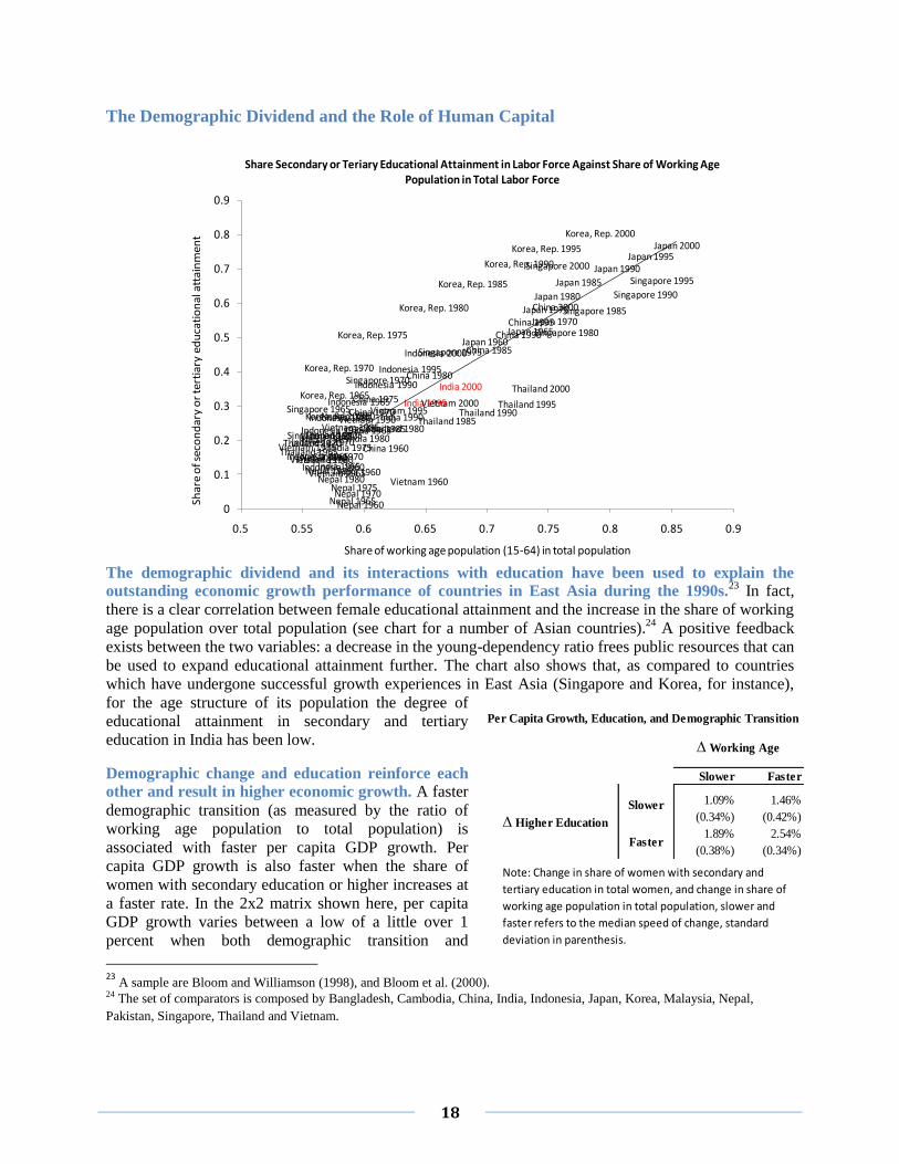
18
The Demographic Dividend and the Role of Human Capital
The demographic dividend and its interactions with education have been used to explain the
outstanding economic growth performance of countries in East Asia during the 1990s.23
In fact,
there is a clear correlation between female educational attainment and the increase in the share of working
age population over total population (see chart for a number of Asian countries).24
A positive feedback
exists between the two variables: a decrease in the young-dependency ratio frees public resources that can
be used to expand educational attainment further. The chart also shows that, as compared to countries
which have undergone successful growth experiences in East Asia (Singapore and Korea, for instance),
for the age structure of its population the degree of
educational attainment in secondary and tertiary
education in India has been low.
Demographic change and education reinforce each
other and result in higher economic growth. A faster
demographic transition (as measured by the ratio of
working age population to total population) is
associated with faster per capita GDP growth. Per
capita GDP growth is also faster when the share of
women with secondary education or higher increases at
a faster rate. In the 2x2 matrix shown here, per capita
GDP growth varies between a low of a little over 1
percent when both demographic transition and
23
A sample are Bloom and Williamson (1998), and Bloom et al. (2000). 24 The set of comparators is composed by Bangladesh, Cambodia, China, India, Indonesia, Japan, Korea, Malaysia, Nepal,
Pakistan, Singapore, Thailand and Vietnam.
China 1960
China 1965
China 1970China 1975
China 1980
China 1985
China 1990China 1995
China 2000
India 1960India 1965India 1970
India 1975India 1980
India 1985India 1990
India 1995
India 2000
Indonesia 1960Indonesia 1965
Indonesia 1970Indonesia 1975
Indonesia 1980
Indonesia 1985
Indonesia 1990
Indonesia 1995
Indonesia 2000Japan 1960
Japan 1965Japan 1970
Japan 1975Japan 1980
Japan 1985
Japan 1990Japan 1995
Japan 2000
Korea, Rep. 1960
Korea, Rep. 1965
Korea, Rep. 1970
Korea, Rep. 1975
Korea, Rep. 1980
Korea, Rep. 1985
Korea, Rep. 1990
Korea, Rep. 1995
Korea, Rep. 2000
Nepal 1960Nepal 1965Nepal 1970
Nepal 1975Nepal 1980
Nepal 1985
Nepal 1990
Nepal 1995
Nepal 2000
Singapore 1960
Singapore 1965
Singapore 1970
Singapore 1975
Singapore 1980
Singapore 1985
Singapore 1990
Singapore 1995
Singapore 2000
Thailand 1960Thailand 1965Thailand 1970
Thailand 1975Thailand 1980
Thailand 1985Thailand 1990
Thailand 1995
Thailand 2000
Vietnam 1960Vietnam 1965
Vietnam 1970Vietnam 1975
Vietnam 1980Vietnam 1985
Vietnam 1990Vietnam 1995
Vietnam 2000
0
0.1
0.2
0.3
0.4
0.5
0.6
0.7
0.8
0.9
0.5 0.55 0.6 0.65 0.7 0.75 0.8 0.85 0.9
Shar
e o
f sec
on
dar
y o
r te
rtia
ry e
du
cati
on
al a
ttai
nm
ent
Share of working age population (15-64) in total population
Share Secondary or Teriary Educational Attainment in Labor Force Against Share of Working Age Population in Total Labor Force
Slower Faster
1.09% 1.46%
(0.34%) (0.42%)
1.89% 2.54%
(0.38%) (0.34%)
Note: Change in share of women with secondary and
tertiary education in total women, and change in share of
working age population in total population, slower and
faster refers to the median speed of change, standard
deviation in parenthesis.
Per Capita Growth, Education, and Demographic Transition
∆ Higher Education
Slower
Faster
∆ Working Age

19
improvements in women‟s education are slow, and 2.5 percent when both of them are fast. In terms of
demographic transition India will be on a fast track soon – an education push could allow it to take full
advantage of this.
Growth prospects and education scenarios
Looking at historical cross-country experience, we can now quantify to what extent education could
contribute to the economic growth prospects of India. We start by estimating a regression model using
panel data for 118 countries for the period 1970-2000 in five-year intervals. The model links growth in
GDP per capita to the investment rate, the initial level of income per capita, the growth rate of population
by educational attainment (population without education, with primary education, and secondary or
higher education), the proportion of working age population with different educational attainment levels
and the interaction between these proportions and the initial level of income per capita. This model
corresponds to specifying a production function for GDP assuming that the productivity of the labor input
differs by educational attainment and that education plays a role in technology adoption (and thus in the
speed of income convergence) and innovation.25
Using the parameters of the estimated model, we compute projections of income per capita for
India under different scenarios concerning the future dynamics of educational attainment levels. We compute three different scenarios based on the following:
(a) assuming that the investment in education is aimed at keeping enrolment rates constant
(constant enrolment rate – CER scenario),26
(b) assuming that enrolment levels in India follow the trend observed in our global database,
which would require a sizable increase over the current level of public investment in
education (global education trend – GET scenario),
(c) assuming that the effort in expanding education leads to a similar educational attainment (in
terms of proportions of population with
different attainment levels) in India in
2040 as that of Korea in 2000, i.e. 2% of
the working age population without formal
education, 11.5% with primary schooling
and 86.5% with junior secondary or higher
(Korea scenario).
The per capita income differences associated with
higher investment in education can be sizable. The
GET scenario implies higher levels of income of around
6 percent by 2040 compared with the CER scenario.
Even better, if a major push were to be made to
improve the structure of educational attainment in India
over the next three decades to resemble that of Korea in
2000, the resulting income level in India would be over
25 See Benhabib and Spiegel (1994) for a similar approach to the role of education in economic growth, based on the seminal
work by Nelson and Phelps (1966). The panel structure allows us to (at least partly) overcome the potential endogeneity of
educational attainment in economic growth regressions. Should increases in income lead to a higher demand for educational
services, the effect in educational attainment of individuals in working age (that is, from 15 to 64 years of age) would not exist in
the following five years, which is the periodicity used in our panel. 26
This should be seen as a lower-bound reference scenario with little practical relevance: there is little doubt that recent rapid
increases in enrolments will continue.
0%
20%
40%
60%
80%
100%
120%
140%
160%
180%
2020 2030 2040
CER GET Korea
Per Capita Income under Different Education Scenarios(percentage difference with respect to income per capita in 2005)

20
16 percent higher than that of the CER scenario by 2040.27
These results indicate important macroeconomic returns to investments in education. The window
of opportunity which opens with the ongoing changes in age structure offers a particularly suitable
moment to utilize such investments, which should also be aimed at reducing the existing disparities across
sexes in terms of educational attainment and to improve the quality of education.
Some caveats should be pointed out, however. The main criticism that could be directed against this
analysis is the lack of adjustment for quality of education in our database, which looks only at the years of
attendance of a particular level of schooling but not at the skills and knowledge actually imparted during
those years. While data that compares educational outcomes in India with those in other countries is not
directly available, there are indications that the quality of education for both primary and secondary
schooling in India lags behind the group of Asian comparators. This would increase the size of the
mountain to climb for India‟s human capital to catch up with that of fast-growing countries in Asia. In
addition, as in most long-run growth projections, it is assumed that the increased supply of skilled labor is
fully absorbed. Doubts concerning whether such job opportunities would exist, given that the economic
expansion in India has been biased toward the modern service sector, have been put forward in several
publications.28
New strategies involving the expansion of selected manufacturing activities would thus be
necessary to accommodate the increasingly educated labor force in the coming decades.
V. The Goods and Service Tax – a Flagship Initiative
Indian central and state governments have been discussing the introduction of a Goods and
Services Tax (GST) to replace the current value-added taxation of the past four years. While there
remain differences over important aspects of the design and implementation of the tax, chances are that
the debate will conclude in time for implementation at the beginning the next fiscal year, in April 2011.
This would be another major step towards improving the tax system, in a series spanning the last two
decades.
Objectives of GST Reform
There are many deficiencies in the current system of indirect taxation, which the introduction of
GST aims to address. These include:
The CENVAT is levied on goods manufactured in India and does not cover value addition in
goods beyond the manufacturing stage;
Only a limited number of services are taxed by the center and none by the states because of
constitutional limitations;
The partial coverage of central and states‟ taxes contributes to tax cascading, and;
The existence of exemptions and multiple rates and the irrational structure of levies make the tax
system complex. Poor infrastructure for tax administration increases the costs of compliance and
undermines revenue collection.
Studies have been conducted to show the likely impact of the implementation of the GST on growth
and tax buoyancy. The National Council for Applied Economic Research (NCAER) estimated that the
27 This assumes growth would increase from the high rate achieved in the first decade of the millennium. Per capita growth rates
rise from around 3.8 percent per year in the 2000s to 4 percent in the 2010s, 4.8 percent in the 2020s, and 5.4 percent in the 2030s
as the demographic dividend gathers force. Per capita income would be 1.5 times higher in 2040 compared with 2005 in the CER
scenario, 1.6 times higher in the GET scenario, and 1.7 times higher in the Korea scenario. 28 See for example Bosworth et al. (2007).

21
implementation of GST would enhance India‟s GDP by 0.9-1.7 percent and gains in exports and imports
would be 3.2-6.3 percent and 2.4-4.7 percent, respectively. Estimates for the rates at which the
introduction of GST would be revenue neutral are 6.2-9.2 percent (NCAER) and 11 percent (5 percent for
central government GST and 6 percent for state government GST, according to the Thirteenth Finance
Commission (FC).
Roadmap and Progress towards GST
While both the central and state governments agree on the desirability of GST, discussions are
ongoing regarding the modalities. These include the framework, the rates structure, taxes to be
subsumed under the new GST, the list of items to be exempted, the treatment of interstate services,
thresholds limits, and tax administration. Constitutional changes will be required to enable the central
government to levy taxes beyond the manufacturing stage and to empower the states to levy taxes on
services. An institutional mechanism needs to be built to ensure compliance.
The first discussion paper on the GST was presented by an Empowered Committee (EC) in
discussions with the government of India (GOI) in November 2009. The discussion paper encouraged
a public debate on the proposed design and implementation modalities of the GST. Based on this, the
Thirteenth FC made recommendations on the design and operational modalities of the GST, as listed
below.
Recommendations Regarding Structure
A single positive rate on all goods and services.
Exports and interstate transactions zero rated,
imports subject to GST on the destination principle.
All indirect taxes and cesses should be subsumed
under the GST.
Petroleum products and natural gas should be taxed
under the GST while additional levies could be
charged by both central and state governments.
A common list of exemptions applicable to all
states.
A threshold of Rs.10 lakh minimum turnover and a
composition limit of Rs.40 lakh should be upheld.
Recommendations Regarding Implementation
All state GST laws should be harmonized and
adopted simultaneously.
Have combined checkpoints at interstate borders.
Have an enforcement mechanism for implementing
the GST and preventing deviations.
A grant of Rs.50,000 crore should be made
available for compensation for the losses made by
some states under the GST.
A system for redress of grievances should be put in
place.
Effective refund systems have to be built by the
states.
GST Framework - Current Status
The central and state governments seem to have come to an agreement that the GST will be a dual
tax with both central and state components levied on the same tax base. The central government has
prepared a constitutional amendment bill which contains proposals for a GST Council29
and a dispute
settlement authority. There is also an agreement that the central government will not have veto powers in
the GST Council and that any changes in the structure of GST would require the approval of two thirds of
the council. The finance minister, meeting with the empowered committee of state finance ministers in
July 2010, suggested the structure of GST and addressed other issues raised by states, as follows:
The centre has suggested to adopt a dual rate structure for goods at the inception of GST and to
adopt a phased approach towards a single rate structure with unification of the rate for goods and
services;
29 The proposed Goods and Services Tax Council, comprising the finance minister, minister of state for finance and state finance
ministers, will have powers to determine the tax rates, list exempted items and decide other issues in the GST regime.

22
The exemption threshold for both goods and services under both central and states‟ GST to be
uniform at Rs.10 lakh;
Exemptions under central excise to be aligned with current exemptions under VAT, which would
ensure alignment of central and states‟ GST exemptions;
As per the Thirteenth FC recommendations, states would be compensated for an initial four years
for loss of VAT and purchase-tax revenues, and;
Setting up of Empowered Group, under Mr. Nandan Nilekani, to decide upon IT infrastructure of
central and state governments to simplify and reduce government-taxpayer interface.
The Challenges Ahead
The state governments are mainly concerned about losing their fiscal autonomy and a possible
accentuation of the vertical imbalance with the implementation of GST. Loss of autonomy would
result from a loss of power to change tax rates, and an accentuation of the vertical imbalance would
increase the states‟ dependence on central government transfers. Currently, over 60 percent of the states‟
own revenue accrues from VAT, and the loss of autonomy would imply a significant reduction in fiscal
maneuverability.
Discussions are continuing about the level of GST rates that would be revenue neutral. The revenue-
neutral rates proposed in the studies cited above are rejected as too low by many state governments.
While the Thirteenth FC has proposed a fund for compensation for potential losses, state governments are
concerned that compensation would be paid only during the transition, while losses could be long-lasting.
The third point of disagreement is over the taxes to be subsumed under the GST. The central
government has suggested entry and purchase taxes be subsumed under the GST. Some state governments
derive substantial revenues from these taxes and do not agree to give them up. State governments differ
also on the treatment of natural gas. While the governments of gas producing states would like to keep
royalties and other taxes outside the GST regime (because they would lose out under the destination
principle), the governments of importing states are concerned about the cascading effect of taxes and want
them to be a part of the GST.
Much work is still needed to make sure that the GST law clarifies the distinction between goods and
services. In addition, a strong mechanism for harmonization of tax laws and administrative procedures is
needed to simplify compliance and enforcement. It is also necessary to ensure that inter-state differences
in policies and procedures do not generate additional economic distortions. Success of the GST would
also hinge upon the level of IT preparedness and awareness at the time of transition.
A Lesson in GST Reform
The experience of a country like New Zealand (NZ) in successfully implementing GST reform shows that having a
single rate with comprehensive coverage of all goods and services helps to keep the rate low. The way in which NZ
introduced GST also gives a lesson in the political economy of reform for any democratic country to follow. NZ‟s
finance minister Bill English attributes the success of GST in his country to five “process elements”: political will,
the right people to design and frame the law; proper packaging of the proposal; effective consultation, and; effective
communication. The key features that enabled the proponents of GST in NZ to go forward were: (i) simplicity, with
a single rate of 10 percent and no exemption; (ii) revenue neutrality; (iii) a wider reform program, comprising
income tax cuts; (iv) abolition of the antiquated wholesale sales tax and increase in welfare payments to offset the
impact of GST on pensioners and low income groups, and; (v) broad consultation. The most difficult component was
“one rate and no exemption”. The effort made in having detailed definitions in place to draw a line between exempt
items and non-exempt items was remarkable and instructive. The public sector was treated like any other
undertaking and the local bodies were paid a part of the revenue raised from taxing local rates.

23
VI. Midterm Appraisal of the Eleventh Five Year Plan
As the implementation of the Eleventh Five Year Plan entered the third year, the National
Development Council issued its midterm appraisal (MTA) in July 2010. The most interesting aspects
of the MTA are its optimism that goals for the level of investment, particularly in infrastructure, could be
met, despite the negative impact of the global financial crisis, and the preview of a massive step-up in
infrastructure spending under the Twelfth Plan. In its review of the macroeconomic framework, the MTA
acknowledges that the original growth target is unlikely to be achieved, and highlights reforms on the
supply side that would support growth.
Infrastructure Investment
The Eleventh Plan recognized the strong need for
robust physical infrastructure to sustain GDP
growth rates of 9-10 percent. The objective was to
raise investment in infrastructure to around 9 percent of
GDP by the end of the Plan, from about 5 percent in the
Tenth Plan. The MTA expresses confidence that most of
the investment of US$514 billion (Rs.20.56 trillion)
envisaged under the Plan would materialize despite the
economic slowdown and lower international capital
flows. Higher-than-anticipated private investment (20
percent) should help offset a projected 13 percent
shortfall in public sector investment.
There are large differences across sectors. The
electricity and telecom sectors will rely more on the
private sector‟s contribution to make up for large public
sector shortfalls. In contrast, revised estimates of
investment in roads by the public sector are 12 percent
higher than the original estimates. Private sector
investment in this sector is set to fall short by 57 percent
due to a shortfall in the award of road projects by the
NHAI during the first three years of the Plan. Revised
estimates indicate a 17 percent increase in infrastructure
investment in airports over the original estimates. While
private sector investment is estimated to be 7 percent
higher than original estimates, public sector investment
is set to be around 40 percent higher. The jump in public
sector investment is due largely to the completion of
airports in Hyderabad and Bangalore.
In both railways and ports the revised estimates are a fraction of original estimates due to slow
progress in awarding PPP projects. The public sector performance in these two sectors has also been
less than expected. Public sector investment is likely to be 9 percent lower in railways and 76 percent
lower in ports. Investments in irrigation, water supply and sanitation are to a large extent carried out by
the government and are estimated to be 10 percent lower than original estimates.
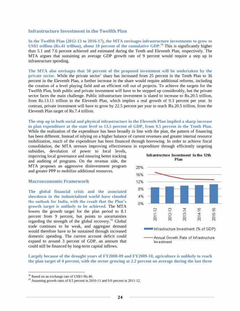
24
Infrastructure Investment in the Twelfth Plan
In the Twelfth Plan (2012-13 to 2016-17), the MTA envisages infrastructure investments to grow to
US$1 trillion (Rs.41 trillion), about 10 percent of the cumulative GDP.30
This is significantly higher
than 5.1 and 7.6 percent achieved and estimated during the Tenth and Eleventh Plan, respectively. The
MTA argues that sustaining an average GDP growth rate of 9 percent would require a step up in
infrastructure spending.
The MTA also envisages that 50 percent of the proposed investment will be undertaken by the
private sector. While the private sector‟ share has increased from 25 percent in the Tenth Plan to 36
percent in the Eleventh Plan, a further increase in the share would require additional reforms, including
the creation of a level playing field and an efficient roll out of projects. To achieve the targets for the
Twelfth Plan, both public and private investment will have to be stepped up considerably, but the private
sector faces the main challenge. Public infrastructure investment is slated to increase to Rs.20.5 trillion,
from Rs.13.11 trillion in the Eleventh Plan, which implies a real growth of 9.3 percent per year. In
contrast, private investment will have to grow by 22.5 percent per year to reach Rs.20.5 trillion, from the
Eleventh Plan target of Rs.7.4 trillion. The step up in both social and physical infrastructure in the Eleventh Plan implied a sharp increase
in plan expenditure at the state level to 13.5 percent of GDP, from 9.5 percent in the Tenth Plan. While the realization of the expenditure has been broadly in line with the plan, the pattern of financing
has been different. Instead of relying on a higher balance of current revenues and greater internal resource
mobilization, much of the expenditure has been financed through borrowing. In order to achieve fiscal
consolidation, the MTA stresses improving effectiveness in expenditure through efficiently targeting
subsidies, devolution of power to local levels,
improving local governance and ensuring better tracking
and auditing of programs. On the revenue side, the
MTA proposes an aggressive disinvestment program
and greater PPP to mobilize additional resources.
Macroeconomic Framework
The global financial crisis and the associated
slowdown in the industrialized world have clouded
the outlook for India, with the result that the Plan’s
growth target is unlikely to be achieved. The MTA
lowers the growth target for the plan period to 8.1
percent from 9 percent, but points to uncertainties
regarding the strength of the global recovery.31
Global
trade continues to be weak, and aggregate demand
would therefore have to be sustained through increased
domestic spending. The current account deficit could
expand to around 3 percent of GDP, an amount that
could still be financed by long-term capital inflows.
Largely because of the drought years of FY2008-09 and FY2009-10, agriculture is unlikely to reach
the plan target of 4 percent, with the sector growing at 2.2 percent on average during the last three
30 Based on an exchange rate of US$1=Rs.40. 31
Assuming growth rates of 8.5 percent in 2010-11 and 9.0 percent in 2011-12.

25
years. Industrial output growth is also estimated to fall short of the Plan target of 10-11 percent, due to
the global financial crisis.
The MTA discusses a number of areas in which policy reforms could improve the outlook on the
supply side. In the agricultural sector, these policy reforms include improved access to water,
replenishment of soil nutrients, access to good quality seeds, reforms in land tenancy, improvements in
agriculture R&D and improvements in agricultural marketing. For industry, the MTA points out that the
lack of infrastructure, especially in power, road and ports has adversely affected its competitiveness. A
major constraint for the Micro, Small and Medium Enterprises (MSME) is access to credit, which could
be overcome through deepening of the financial sector as well as mechanisms for expanding access to
equity financing. To lessen the burden of infrastructural bottlenecks, the MTA encourages “clustering” of
MSME. In addition, the MTA stresses skill development for the unorganized sector through public-
private partnerships, and greater flexibility in labor regulation, which would increase demand for labor in
the organized sector.□

26
Appendix: Education and Growth – a model for income projections
We compute income projections for India in the period 2010-2040 using an estimated panel data regression model
based on a production function approach. In particular, we use the following specification,
,55,, itit
j it
jit
jitititLj
j
j
j it
jit
jity yL
Lyinvg
L
Lg
where gy,it is the growth rate of income per capita in the corresponding 5-year period for country i,
it
j
it
L
L is the share of
population with educational attainment j in the working age population, gLj,it is the growth rate of the working age
population with educational attainment j, invit is the investment rate and yit-5 is the initial level of income in the 5-
year period. The error term, t, is assumed to be composed by a country and a period fixed effect, as well as the
standard random shock, assumed independent across countries and periods.
The model implies that economic growth is affected by factor accumulation, technology innovation and adoption, as
well as income convergence dynamics. Factor accumulation is approximated by the investment rate and the growth
rate of population by educational attainment (thus assuming a production function with differentiated labor input by
education level). We control for conditional income convergence by including the initial level of income per capita.
In the spirit of Nelson and Phelps (1996), we let human capital play a role in the process of technology adoption and
innovation beyond the accumulation effect from the growth rate of population by educational attainment level. This
means that the specification should include also the share of working age population by educational attainment level,
as well as its interaction with the initial income per capita. This last term accounts for the fact that human capital is a
potential determinant of the speed of income convergence by enabling a speedier adoption of foreign technologies
by countries which are far from the technological frontier.
We estimate the model presented above using data for 118 countries, sourced from the Penn World Tables and the
IIASA-VID dataset. The results of the estimation are presented in Table A1. The first column of Table A1 shows the
estimates of a simple model where income per capita growth is assumed to depend exclusively on factor
accumulation. We thus regress income per capita growth on the investment rate and on the growth rate of the
population groups by educational attainment. The parameter estimates imply that investment and the growth rate of
population with at least junior secondary education are the only significant driving forces of economic growth in our
sample. In the second column, we enlarge this simple
specification by adding convergence dynamics through the
inclusion of the initial level of income per capita in the model.
The parameter attached to this variable is significant and
negative, implying convergence of income per capita towards a
country-specific steady state. Finally, the last column of Table
A1 presents the estimates of the model which is further
augmented to include human capital as a determinant of
technology growth. In this specification we also include the
share of individuals with each education level (the technology
innovation term in Benhabib and Spiegel, 1994), as well as its
interaction with the level of development (the technology
adoption term in Benhabib and Spiegel, 1994). The results of the
estimation of this model, which is the one used to obtain the
projections presented in the study, gives evidence of the
importance of human capital as a determinant of economic
growth. On the one hand, as countries expand education,
economic growth effects take place through the change in the
composition of skills in the working age population. On the
other hand, countries which are further away from their
Estimates of the economic growth panel data models
1 2 3
Investment rate 0.234*** 0.273*** 0.321***
[0.0904] [0.0992] [0.0845]
Growth rate pop. (no educ.) -0.00957 -0.0432 -0.0479
[0.0431] [0.0485] [0.0415]
Growth rate pop. (prim educ.) 0.0703 0.02 -0.036
[0.0864] [0.0614] [0.0831]
Growth rate pop. (sec. and tert. educ.) 0.199*** 0.250*** 0.271***
[0.0651] [0.0779] [0.0666]
Proportion with primary ed. 1.603***
[0.607]
Proportion with sec. and tert. ed. 1.169**
[0.494]
Initial income -0.224*** -0.113***
[0.0363] [0.0431]
Initial income Proportion with primary ed. -0.225***
[0.0740]
Initial income Proportion with sec. and tert. ed. -0.128**
[0.0573]
Observations 790 790 790
R-squared 0.121 0.244 0.258
Number of countries 118 118 118
Notes: Dependent variable is the growth rate of GDP per capita. Data ranges from
1960 to 2005 in non-overlapping 5 year periods. Country and period fixed effects
included in all models. Standard deviation in brackets.

27
equilibrium in terms of income per capita tend to profit more from such an education expansion, an effect which is
embodied in the negative coefficient attached to the interaction between initial income per capita and the human
capital variables.

28
India: Selected Economic Indicators
2006/07 2007/08 2008/09 2009/10 2010/11 2011/12
Est Proj Proj
Real Income and Prices (% change)
Real GDP (at factor cost) 9.6 9.3 6.8 8.0 8.6 9.0
Agriculture 4.2 5.8 -0.1 0.4 5.4 3.0
Industry 12.2 9.7 4.4 8.0 8.1 9.5
Of which : Manufacturing 14.3 10.3 4.2 8.8 8.8 9.5
Services 10.1 10.3 10.1 10.1 9.6 10.2
Prices (average)
Wholesale Price Index 5.5 4.5 8.3 3.5 7.5 6.0
Consumer Price Index 6.4 6.2 9.1 12.5 … …
Consumption, Investment and Savings (% of GDP)
Consumption 67.4 65.9 70.6 68.7 69.3 70.0
Public 10.3 10.3 11.0 12.0 11.3 11.3
Private 57.0 55.6 59.5 56.7 58.0 58.8
Investment 35.7 38.1 34.5 36.5 34.4 35.9
Public 8.3 8.9 9.5 8.4 10.6 9.8
Private 26.5 27.9 24.6 25.6 22.0 26.2
Gross National Savings 37.0 39.8 35.3 36.9 32.7 32.5
Public 3.6 5.0 0.5 2.1 3.8 5.7
Private 31.0 31.9 31.7 31.6 28.9 26.9
External Sector
Total Exports (% change in current US) 24.5 26.6 13.3 -5.1 11.9 17.0
Goods 22.6 28.9 13.7 -3.6 15.0 15.0
Services 28.0 22.4 12.5 -7.8 6.0 19.5
Total Imports (% change in current US) 22.7 31.6 16.4 -0.2 13.6 15.0
Goods 21.4 35.1 19.4 -2.7 15.1 15.4
Services 28.5 16.2 1.1 14.5 6.0 12.9
Current Account Balance (% of GDP) -1.0 -1.3 -2.4 -2.8 -2.9 -3.2
Foreign Investment (US billion) 14.8 43.3 3.5 52.1 57.0 48.0
Direct Investment, net 7.7 15.9 17.5 19.7 28.0 27.0
Portfolio Investment, net 7.1 27.4 -14.0 32.4 29.0 21.0
Foreign Exchange Reserves (excl. Gold) (US billion) 191.9 299.2 241.4 259.7 301.0 330.7
(in months of goods and services imports) 9.8 11.6 8.1 8.7 8.9 8.5
General Government Finances (% of GDP)
Revenue 20.0 21.0 19.9 17.4 17.6 19.1
Expenditure 25.4 26.0 28.7 26.4 25.2 26.5
Deficit 5.4 5.0 8.8 9.0 7.7 7.4
Total Debt 77.2 74.0 75.0 71.6 67.7 67.1
Domestic 72.3 69.6 70.2 67.4 63.2 63.1
External 4.9 4.3 4.8 4.2 4.5 4.0
Monetary Sector (% change)
Money Supply (M3) 21.5 21.2 19.1 16.7 16.2 16.6
Domestic Credit 20.2 17.7 23.4 20.2 20.2 16.1
Bank Credit to Government 8.0 8.7 42.0 30.5 25.3 15.8
Bank Credit to Commercial Sector 25.7 21.1 16.9 15.9 19.7 16.3
Sources: Central Statistical Organization, Reserve Bank of India, and World Bank Staff Estimates.

29
References
Aitken, Brian, Gordon Hanson and Ann Harrison (1997), “Spillovers, Foreign Investment and Export
Behavior,” Journal of International Economics 43, pp. 103–142.
Alvarez, Roberto and Ricardo Lopez (2006), “Is Exporting a Source of Productivity Spillovers?”
unpublished manuscript, Central Bank of Chile and Indiana University.
Barrios, S., H. Gorg and G. Strobl (2003), “Explaining Firms‟ Export Behaviour: R&D, Spillovers, and
the Export Market,” Oxford Bulletin of Economics and Statistics 65.
Basu, Kaushik (2010) "The Economics of Foodgrain management in India", New Delhi: Ministry of
Finance, Government of India, available at 'http://finmin.nic.in/WorkingPaper/Foodgrain.pdf'
Benhabib, J. and M. Spiegel (1994) The Role of Human Capital in Economic Development: Evidence
from Aggregated Cross-Country Data. Journal of Monetary Economics 34: 143-173.
Berg, Andrew, Jonathon Ostry and Jeromin Zettelmeyer (2008), „What Makes Growth Sustained?‟ IMF
Working Paper Series 08/59, International Monetary Fund, Washington, DC, March.
Bernanke, Ben S. (2005), “The Global Saving Glut and the US Current Account Deficit”, remarks at the
Sandridge Lecture, Virginia Association of Economics, Richmond, Virginia (March).
Bernard, A.B. and J.B. Jensen (2004), “Why Some Firms Export,” Review of Economics and Statistics
96, pp. 561–569.
Bloom, D. and J. Williamson (1998) Demographic Transitions and Economic Miracles in Emerging Asia.
World Bank Economic Review 12: 419-56.
Bloom, D., D. Canning and P. Malaney (2000) Demographic Change and Economic Growth in Asia.
Population and Development Review 2000 26: 257-290.
Bosworth, B., S.M. Collins and A. Virmani (2007) Sources of Growth in the Indian Economy. India
Policy Forum 3: 1–50.
Dev, Mahendra and N. Chandrasekhara Rao (2010) " Agricultural Price Policy, Farm Profitability and
Food Security”. Economic and Political Weekly, June, New Delhi.
Eichengreen, Barry (2008), “The Real Exchange Rate and Growth”, Commission on Growth and
Development Working Paper No. 4
Haddad, Mona and Cosimo Pancaro (2010), “The Role of Real Exchange in Boosting Growth in
Developing Countries”, Mimeo, Washington, DC: The World Bank.
Hale, Galina and Cheryl Long (2006), “Firm Ownership and FDI Spillovers in China,” unpublished
manuscript, Federal Reserve Bank of San Francisco and Colgate University (April).
Hausmann, Ricardo., Lant. Pritchett and Dani Rodrik (2005), „Growth Accelerations‟, Journal of
Economic Growth, 10, 303-329.
Heston, A., Robert Summers and Bettina Aten, Penn World Table Version 6.3, Center for International
Comparisons of Production, Income and Prices at the University of Pennsylvania, August 2009.

30
IIF (2010), “Capital Flows to Emerging Market Economies”, IIF Research Note, October 4th
2010 International Study Group on Exports and Productivity (2008), Understanding Cross-Country Differences
in Exporter Premia: Comparable Evidence from 14 Countries, Review of World Economics, Vol.
144, No. 4, 596-635.
Johnson, S., J. D. Ostry, and Arvind Subramanian (2007), “The Prospects for Sustained Growth in Africa:
Benchmarking the Constraints”, IMF Working Papers No. 52, Washington, DC: IMF.
Jones, Benjamin F. and Benjamin A. Olken (2005), “The Anatomy of Start-Stop Growth,” NBER
Working Paper No. 11528.
KC, S., B. Barakat, A. Goujon, V. Skirbekk, W. Sanderson and W. Lutz (2010) Projection of Populations
by Level of Educational Attainment, Age and Sex for 120 Countries for 2005-2050.
Demographic Research 22:383-472.
Koenig, P. (2005), “Agglomeration and the Export Decision of French Firms,” CREST Working Paper
No. 2005-01.
Kokko, A., M. Zejan and R. Tansini (2001), “Trade Regimes and Spillover Effects of FDIs: Evidence
from Uruguay,” Weltwirtschaftsliches Archiv 137, pp. 124– 149.
Krause, L. (1987), “The Structure of Trade in Manufactured Goods in the East and Southeast Asian
Region”, in: Bradford, C. and William Branson, Trade and Structural Change in Pacific Asia,
Chicago: University of Chicago.
Krueger, A.O. (1998), Why trade liberalization is good for growth, Economic Journal Vol. 108, issue
450, pp. 1513-1522.
Lawless, Martina (2005), “Firm Export Participation: Entry, Spillovers and Tradability,” unpublished
manuscript, Central Bank and Financial Services Authority of Ireland (November).
Levy-Yeyati, Eduardo and Francessco Sturzenegger (2007), „Fear of appreciation‟, World Bank Policy
Research Working Paper No. 4387, Washington, DC, 1 November.
Lin, Jane C. (2004), “General Agglomeration Externalities, Export Spillovers, and Firm Behavior: A
Study of the Electronics Industry in Taiwan over the 1986–96 Period,” unpublished Ph.D.
dissertation, Columbia University.
Miao, Yanliang and Andrew Berg (2010), "The Real Exchange Rate and Growth Revisited: The
Washington Consensus Strikes Back?," IMF Working Papers 10/58, International Monetary
Fund.
Ministry of Finance (2010), Economic Survey 2009-10, New Delhi.
Montiel, Peter J. and Luis Servén, (2008), "Real Exchange Rates, Saving and Growth: Is there a Link?,"
Department of Economics Working Papers 2010-20, Department of Economics, Williams
College.
Nelson, R., and E. Phelps (1966), Investment in Humans, Technological Diffusion, and Economic
Growth. American Economic Review 56: 69-82.

31
Ostry, J.D., Atish Ghosh, Karl Habermeier, Marcos Chamon, Mahvash Qureishi, and Dennis B.S.
Reinhardt (2010), Capital Inflows: The Role of Controls, IMF Staff Position Note SPN 10/04,
Washington, DC.
Polterovich, Victor and Vladimir Popov, (2003), "Accumulation of Foreign Exchange Reserves and Long
Term Growth," MPRA Paper 20069, University Library of Munich, Germany.
Population Division of the Department of Economic and Social Affairs of the United Nations Secretariat,
World Population Prospects: The 2008 Revision, http://esa.un.org/unpp, Saturday, September 25,
2010; 5:16:14 PM.
Razin, Ofair. and Susan M. Collins (1999), „Real Exchange Rate Misalignments and Growth.
International Economic Integration: Public Economics Perspectives‟, in A. Razin and E. Sadka
(eds), International Economic Integration: Public Economics Perspectives, Cambridge, UK:
Cambridge University Press.
Rodrik, Dani (2006), “Industrial Development: Stylized Facts and Policies,” unpublished manuscript,
Kennedy School of Government (August).
Rodrik, Dani (2008), “The Real Exchange Rate and Economic Growth”, Brookings Paper on Economic
Activity, Fall 2008.
Woodford, (2009), Is an Undervalued Currency the Key to Economic Growth? Discussion Paper No.:
0809-13, Columbia University, New York.
World Bank (2010a), India Economic Update June 2010, World Bank, New Delhi.
World Bank (2010b), “Developing Trends: November 2010”, Development Prospects Group, Washington
DC.