indexing techniques for temporal text containment queries
TRANSCRIPT
Indexing Techniques for Temporal Text Containment Queries
Sharath Srinivas University of Maryland, College Park
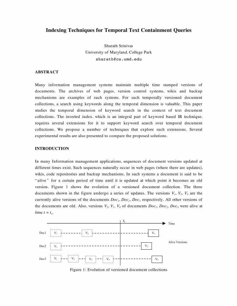
ABSTRACT Many information management systems maintain multiple time stamped versions of documents. The archives of web pages, version control systems, wikis and backup mechanisms are examples of such systems. For such temporally versioned document collections, a search using keywords along the temporal dimension is valuable. This paper studies the temporal dimension of keyword search in the context of text document collections. The inverted index, which is an integral part of keyword based IR technique, requires several extensions for it to support keyword search over temporal document collections. We propose a number of techniques that explore such extensions. Several experimental results are also presented to compare the proposed solutions. INTRODUCTION In many Information management applications, sequences of document versions updated at different times exist. Such sequences naturally occur in web pages (where there are updates), wikis, code repositories and backup mechanisms. In such systems a document is said to be “ alive ” for a certain period of time until it is updated at which point it becomes an old version. Figure 1 shows the evolution of a versioned document collection. The three documents shown in the figure undergo a series of updates. The versions V3, V2, V5 are the currently alive versions of the documents Doc1, Doc2, Doc3 respectively. All other versions of the documents are old. Also, versions V2, V1, V4 of documents Doc1, Doc2, Doc3 were alive at time t = ts.
Figure 1: Evolution of versioned document collections
ts
V1 Doc1
Time
V3
Doc2 V1
Doc3 V1 V5
V2
V2
V2 V3 V4
Alive Versions

For temporal document collections, a search involving both the text and the time (temporal text containment query) is valuable. Current Information Retrieval techniques, which support efficient keyword search over document collections are not well suited to support a search involving both keywords and the temporal specification. In order to support search involving both keywords and time two approaches can be taken. The first approach is to search on the most recent version of the documents. Though time is not a dimension of the search query in this approach, only currently alive documents are searched. The past versions of the document are not retrieved, even if they were highly relevant to the query. In the second approach, different versions of the document are treated as independent documents and are indexed separately. Though this technique can retrieve any version of a document that is most relevant to the query, it cannot support queries involving time as one of the search dimensions. The ability to archive and retrieve any version of a document from a collection of versioned documents is very important. Many information exchange mediums like the web and the Wiki are ephemeral because of constant updates and a development environment that is collaborative. Unless an effort is made to archive the temporal data, it might be lost permanently because of overwrites by newer versions. Archiving of versioned document collections is an important problem and has received significant attention in the recent times [1, 2]. Though archiving of temporal data has been a well-studied problem, the equally important problem of retrieving data from such archives has not been significantly addressed. The primary requirement of a temporal text containment query technique is that it should be able to support search along two dimensions: terms and time. Further, it should be able to retrieve any version of the document that closely matches the user-specified search dimensions. The queries over temporal document collections can be classified into the following three types:
I. Given a set of keywords find all the relevant documents, possibly ranked by their relevance to the query.
II. Given a set of keywords and a time slice t, find the relevant documents alive during t. III. Given the keywords and a time range [ts, te), find all the relevant documents that were
alive during this time range. Since keywords are the most effective manner for the users to express what they are looking for in document collections, it is included in all the three query types. The only difference among the three query classes is the inclusion/ non-inclusion of the time dimension or in the type of queries along the time dimension (point or range queries).

For fast retrieval of documents that contain terms in the user query, an index over the terms in the documents needs to be built. The inverted index [3] is the most widely used indexing technique in search engines. It is a data structure that efficiently stores for each distinct term in the document collection, the list of all documents that contain the term. Apart from this information, the inverted index can store a few other information like the frequency of occurrence of the terms in a document and also position of the terms inside the documents. This additional information can help in ranking the search results when there are more than one result that match the user query. In its simplest form, the inverted index correspond to a set of documents D = {D1, D2,…, Dn}, where Di represents the document identifier. If T = {T1, T2,…Tm} represents the set of all distinct terms in D, a B+ tree is built over T. This B+ tree, which is called the Vocabulary, maps each term to its idf score and an inverted list of postings. Each posting stores the document identifier and other information about the term, called its payload. Thus, each posting in the inverted list is of the form < di , p>, where p represents the payload corresponding to a term ti in a document di. The structure of inverted index is as shown in Figure 2.
Figure 2: Inverted index organization
The simple B+ tree vocabulary when extended to index temporally versioned document sequences has a major problem. The B+ tree is built using only the document terms as the key and thus can only search using keywords. It does not support time as one of the search dimensions. In Section 3, we propose several solutions to handle this problem. The rest of this paper is organized as follows, in Section 2, we discuss the related work in the area of full text indexing, multi-dimensional data indexing and temporal data management. In Section 3, we present the techniques that we have explored for answering temporal text containment queries. The experimentation results of the techniques presented in Section 3 are provided in Section 4. Finally in Section 4, we conclude this paper.
Vocabulary
Tm
t2
T1
Inverted List of terms
Document Collections
Abc….
T1, < d1, p > T1, < d2,p > . . . Tm
B+ tree
Inverted list
d1, p
d2, p

2. RELATED WORK In this section we review the recent work in the area of full text indexing, multidimensional indexing, temporal databases and temporal storage and retrieval, all of which form the basis of our work. 2.1. Full Text indexing In any IR technique, the user issues a query and all documents containing terms in the query are retrieved. Though all the documents can be sequentially scanned to find terms in the user query, this technique is very inefficient for large document collections. So, all IR techniques use some form of indexing to speed up the search. In full text indexing, almost every word in the document is used as an index term. The most popular full text indexing methods are inverted index [3, 4] and signature files [5]. The other indexing technique which is widely used and which is not a full text indexing technique is Latent Semantic indexing (LSI) [6, 7]. In the inverted index, for each term, the list of all documents in which the term was contained and additional information like the frequency of the occurrence of the word in the document are stored. The terms are organized as a B+ tree for fast lookup. When a search is performed, the B+ tree storing the terms is queried with each term in the user query. The size of the inverted index can be huge for large document collections. Several works like [5] address the issue of compressing the inverted index. Since most of the space in the inverted index is utilized for storing document IDs and offsets, integer compression techniques can be used to restrict the size of the inverted index. In the signature file approach to indexing text, every word is assigned a bit pattern of size F with m bits set to 1 and others set to 0. The word signature is calculated using a hash function. The signature of the entire document is calculated as the logical OR of all the signatures of the words present in the document. Every query issued by the user is also assigned a signature. The query is processed by matching its signature against that of the document. False positives can occur if a query signature matches a document signature, but the word is not in the document. The signature files are less widely used because of issues in the index size and the false positive rate. Another popular Information Retrieval technique is the Latent Semantic Indexing (LSI). In most IR techniques, the terms in the documents and the query terms are literally matched. Such techniques fail to recognize synonymy (multiple words having the same meaning) and polysemy (words having multiple meanings). This problem is addressed in LSI, where a document and a query can have high cosine similarity even if they do not share common terms. In LSI, a low rank Singular Value Decomposition (SVD) of the document-term matrix is obtained. The projection into the latent semantic space is chosen such that the representations in the original space are changed as little as possible when measured by the sum of the squares of the differences. For a more detailed survey on LSI refer to [6].

2.2. Multidimensional Indexing Multidimensional indexing structures are data structures that support indexing and retrieval of objects that have more than dimension. Multidimensional data include points, line segments, rectangles, and polygons in 2D, 3D or higher. Storage and retrieval of multidimensional data is important in many business, scientific and engineering application. Multidimensional access methods can be classified into Point Access Methods (PAM) and Spatial Access methods (SAM) [8]. PAM is primarily designed to index and search multidimensional points that do not have any spatial extension. SAM is designed for objects that have spatial extent like lines, polygons or higher dimensional polyhedron. Some popular PAM include Grid files [9], Quad-trees [10] and kd- trees [11]. The grid file is a multidimensional array used as an index to objects that have multiple dimensions. This method is based on hashing and guarantees that any record can be retrieved by at most two-disk access. This is done by making use of a grid directory consisting of grid blocks and all records in a block are stored in the same bucket. The grid itself is maintained in the main memory and is represented as d one-dimensional arrays called scales. In Quad-trees, every internal node conceptually represents a square and it has four children. The four children represent the four quadrants of the square. The quad tree is recursively defined: split the current data into four quadrant and recursively construct quad-trees for each quadrant. In kd-trees, at each intermediate node, the k-dimensional space is split into two parts by a (k-1) dimensional hyperplane. The direction of the split alternates between the k possibilities from one tree level to the next. The most popular SAM techniques include R trees [12] and R+ trees [13]. In R-trees, a set of hierarchically nested Minimum Bounding Rectangles (MBR) is maintained. Each node of the R-tree stores a variable number of elements. Each element stores a way of identifying the child node and a MBR of all the elements inside the child node. R+ trees are an extension of the R-trees, wherein overlapping of internal node is avoided by inserting an object into multiple nodes if necessary. 2.3. Temporal Databases Temporal databases are databases where time is a first class object. They have a temporal data model and a temporal version of structured query language (SQL). Traditional relational databases are sometimes known as snapshot databases because they do not keep the history of the relations. In contrast, temporal databases make use of temporal attributes to record the history of the tuples. The tuples are never deleted and they are versioned to maintain their history. Temporal databases can be classified as Transaction-time databases [14], Valid Time databases [15] or bitemporal databases. Transaction time is defined as the time when a fact is stored in the database. In transaction time databases, history of the database activity is

recorded rather than the real world history. Valid time is defined as the time when a fact becomes valid in real life. The valid time database stores the entire temporal behavior of an object. Bitemporal data denotes both the valid time and transaction time of the data. A bitemporal database combines the features of both the transaction and the valid databases. In a transaction-time database, both the current and the past data needs to be maintained. Thus, an object deletion is logical in nature, and not physical. (i.e., A tuple delete operation in the database is treated as an update to the end time of the tuple and not as a physical delete from the disk.) As a result, the database size grows exponentially in size with new updates to the relations. In order to retrieve data from such huge archives, very efficient data structures are necessary. Some of the multi-dimensional data structures discussed in Section 2.3, like quad-trees, kd-trees and R+ trees are used for this purpose. In valid-time databases, the past states of an object are not kept. When an object deletion occurs, the corresponding object is physically deleted from the database. The database and the index sizes of valid time databases are much more manageable compared to transaction time databases. For a more detailed survey on temporal databases we refer the reader to [16]. 2.4. Temporal Data Retrieval Techniques With the growing amount of archived data both on the Internet as well as local document collections, retrieval of time-stamped data from versioned document collections has received some research attention in the recent years. The pioneer work in this area was done by Anick and Flynn [17]. In their approach, the current versions of the documents are stored as complete versions, and backward deltas are stored for the historic versions. The current versions can be accessed very fast, whereas accessing the previous versions is not very efficient. The V2 temporal database system [18] developed by Norvag makes use of a combination of text indices and time indices to perform efficient text containment queries. A more refined version of the V2 temporal database system with more efficient index space utilization, called Interval based Temporal Text Index (ITTX) [19] was developed by the same authors. In ITTX, an implicit assumption that the past data is less frequently queried compared to the current data is made. Separate indices are maintained for the past and the current data. The past data stores both the start and the end timestamps. The current data stores a single timestamp, denoting the start timestamp of the data. Since there is no end timestamp for current data, access to this data is much faster. When the current data is updated, it is transferred from the current index to the past index and its end timestamp is updated. Text search over temporally versioned document collections such as the web has been studied in [20]. Extensions to the inverted index to support temporal queries are proposed. Approximate temporal coalescing is used to reduce the size of the inverted index. In temporal coalescing adjust versions of the inverted index postings that have similar payloads are merged, while keeping the maximum error bounded. Several optimizations are

made by materialization of the inverted index. Though this technique results in smaller index sizes, it only provides approximate answers to queries, which might not be desirable in many applications. 3. PROPOSED SOLUTIONS The inverted index is an indexing data structure that is currently an integral part of all full text search engines. Any extension made to a text search engine to support temporal term queries clearly requires modifications to the inverted index. In the regular inverted index, a vocabulary B+ tree is maintained which maps the terms to their inverse document frequency (idf) score and an inverted list. The idf score is a measure of the informativeness of the term. The inverted list LT of a term T contains a list of postings of the form <Document ID, term frequency>. The Document ID is a unique identifier that is associated with a document and the term frequency is the frequency of occurrence of T in the document identified by Document ID. It is important to note that for every term T, it has a single idf score, common to the entire document collection. However, the tf scores are document specific and their values can vary across different documents in the same collection. In order to find documents in a ranked order according their relevance to the query a relevance function is necessary. The relevance function used in most search engines is the tf.idf score. Higher tf.idf score is considered to imply higher relevance between the query and the document. When the inverted index is extended to support temporal document collections, it is much more efficient to decouple the tf and the idf scores. This is similar to the technique used in [20]. At a snapshot of time, a term has a single idf score and over time its scores might vary. So, the idf score for a term is essentially a time series. For all the terms in the document collection, we have to manage a collection of time series data. The index to store the idf scores is shown in Figure 3.
Fi
Figure 3: The idf index
The idf scores are easy to maintain, as there is not much data volume involved. In this work, we focus on the more difficult problem of maintaining the tf scores. In the rest of the paper,
time
T2
idf Index

we use the following notation: T represents the terms of the document, Di represents the document identifier, t represents the time at which the document di was alive. The terms in the user queries are represented by Tq. We have persued two different approaches to the problem of indexing temporal document collections. In the first approach, every version of a document is treated as a new document. So, subsequent versions of the same document get different document identifiers even if the changes between them were minimal. Consider two different versions of a document, with document identifiers D1 and D2. A term Ti can occur in both documents D1 and D2. In this case, the term Ti is indexed twice, once as the term Ti belonging to D1 and the next time as the term Ti belonging to D2. This approach simplifies the problem of indexing temporal document collections to a large extent, but the resulting index sizes can be huge. The Vocabulary Index, Hierarchical Vocabulary-Time Index, Multidimensional Index (kd-tree) and the Independent Vocabulary and Time Index techniques explained in the next subsections are consistent with this approach. In the second approach, a document and all its subsequent updates are treated as a single document with multiple versions. In this case, the document D and all its versions v1, v2,…vn are represented as D.v1, D.v2, … , D.vn. If the frequency fi of a term Ti is same in consecutive versions of the same document, the term is added to the index just once with a start time (the time at which term first occurred in document with frequency fi) and the current time as the end time. When the frequency of the term changes from fi to some other value, say fj, its end time corresponding to fi is updated and a new entry corresponding to the frequency value fj is added to the index. The term vs time representation of this approach is Figure 4. This corresponds to a single document and all its revisions. The techniques explained in subsections 3.5. and 3.6. fall under this category.
Figure 4: Time Vs Term representation

3.1. Vocabulary Index In the naïve approach, a vocabulary V containing all the distinct terms in the versioned document set is maintained. For each distinct term Ti in the vocabulary V an inverted list of its postings is maintained. Each posting stores the document Di in which the term was present, the time ti at which the document Di was alive and the frequency fi of the occurrence of the term. Further, the postings for a term are sorted in the order of the frequency of occurrence of the term. The vocabulary V is organized as a B+ tree, for fast lookup of the terms. The organization is as shown in Figure 5.
Figure 5: Vocabulary Index For type I queries the Vocabulary index can be used to find the posting list corresponding to terms in the query. For type II and III queries, after finding the postings list corresponding to a term. The list it has to be filtered to remove the documents that were not alive during the time slice or the interval. The result of all these three query types on the vocabulary index is already sorted on the frequency of occurrence of the term. Though the vocabulary index is highly efficient for keyword-only queries, for queries that involve both keywords and time, they are inefficient, as the posting list has to be linearly searched to find the postings alive during the time mentioned in the query. This requires bringing all the postings from the disk to the memory, which incurs a significant cost. The naïve algorithm to perform a type III query over the vocabulary index is shown in Figure 6.
Input: Term: Tq Time range: (ts, te) Procedure: 1 From the vocabulary index V, find
the posting list P corresponding to Tq
2 For each entry pi = (D, t, f) in P 3 if (ts < t) AND (t < te) 4 Add pi to Result
B+ tree
T2 T1
Vocabulary
D1, t1 , f1 Inverted list
D2, t2 , f2
D1, t1 , f1
D2, t2 , f2
Tn

Figure 6: Algorithm for Type III query over the vocabulary index 3.2. Hierarchical Vocabulary-Time Index The problem with Vocabulary index is that it is not efficient for queries involving both time and keywords. Since time was not a part of the index, all the elements in the posting list had to be linearly searched for the time values mentioned in the query. In order to solve this problem using the Hierarchical Vocabulary-Time (HVT) Index an index is built both on the time as well as the keywords. This approach is similar to the two level AP-Index proposed by Gunadhi and Segev [21]. The structure of the HVT index is shown in Figure 7. In the HVT Index, first a B+ tree on the terms in the documents is built. Each leaf entry Ti of the B+ tree points to an append-only tree indexed on the time called a time index. The leaf entry of the time index points to a posting list (<Document ID, frequency>) sorted on the frequencies.
Figure 7: Hierarchical Vocabulary-Time Index
For type I queries, the vocabulary index can be queried to find the time index that corresponds to a term. The posting list of all the leaves in that time index are then merged and then sorted on the frequency of occurrence of the terms. For type II queries, the vocabulary index is first queried to find the time index corresponding to the term and then the time index is queried on the time slice given in the query. This returns the results sorted on the frequency of occurrence of the term. For type III queries, involving keyword and a time range [ts, te) the same procedure like before is followed, but the only change is that the posting lists corresponding to ti > ts and ti < te are merged and then sorted on frequency fi. The algorithm to perform Type III queries on HVT index is shown in Figure 8.
……… tn t2 t1
…Tn T2 T1
Vocab Index
Time Index
Time Index
D1, f1
D2, f2
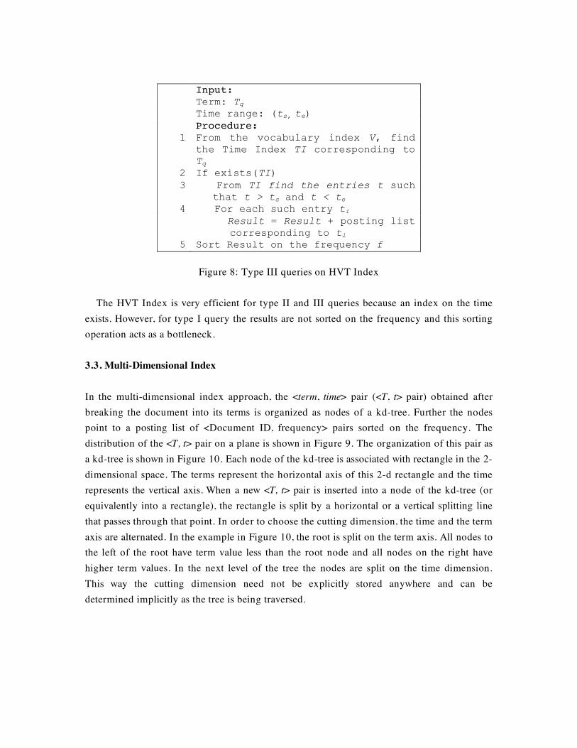
Input: Term: Tq Time range: (ts, te) Procedure: 1 From the vocabulary index V, find
the Time Index TI corresponding to Tq
2 If exists(TI) 3 From TI find the entries t such
that t > ts and t < te 4 For each such entry ti Result = Result + posting list
corresponding to ti 5 Sort Result on the frequency f
Figure 8: Type III queries on HVT Index
The HVT Index is very efficient for type II and III queries because an index on the time exists. However, for type I query the results are not sorted on the frequency and this sorting operation acts as a bottleneck. 3.3. Multi-Dimensional Index In the multi-dimensional index approach, the <term, time> pair (<T, t> pair) obtained after breaking the document into its terms is organized as nodes of a kd-tree. Further the nodes point to a posting list of <Document ID, frequency> pairs sorted on the frequency. The distribution of the <T, t> pair on a plane is shown in Figure 9. The organization of this pair as a kd-tree is shown in Figure 10. Each node of the kd-tree is associated with rectangle in the 2-dimensional space. The terms represent the horizontal axis of this 2-d rectangle and the time represents the vertical axis. When a new <T, t> pair is inserted into a node of the kd-tree (or equivalently into a rectangle), the rectangle is split by a horizontal or a vertical splitting line that passes through that point. In order to choose the cutting dimension, the time and the term axis are alternated. In the example in Figure 10, the root is split on the term axis. All nodes to the left of the root have term value less than the root node and all nodes on the right have higher term values. In the next level of the tree the nodes are split on the time dimension. This way the cutting dimension need not be explicitly stored anywhere and can be determined implicitly as the tree is being traversed.

Figure 9: A distribution of the (term, time) pair on a plane
Figure 10: A kd-Tree for the (term, time) distribution in Figure 7
For type I queries involving only keywords, all nodes to the left of a parent node split on the term dimension has term values less than the parent and all nodes on the right have greater term values. While traversing through the kd-tree only the alternate levels of the tree that are split on the terms are used for traversal and the levels split on the time dimension are not used at all. For type II queries, the levels of the tree split on time and the term dimensions are both used for traversal. For type III queries that involve a time range, the posting list of all matching nodes have to be merged and sorted according to the frequency of occurrence of the term. The run time of the multidimensional index created using kd-trees is O(log n) assuming that the elements are inserted in a random order. However, in our application, the new terms added to the index are in monotonically increasing time order. Thus, the kd-tree index becomes severely unbalanced and the performance is several orders of magnitude slower compared to the balanced kd-tree. The experimentation results in section 4 provide more insights on the compatibility of kd-trees for temporal term data.

3.4. Independent Vocabulary and Time Indices The Independent Vocabulary and Time (IVT) index addresses some of the issues encountered in the previously discussed techniques. In the IVT index approach separate indices are maintained for both the term and the time dimension. The terms in the document are organized as a B+ tree in the vocabulary index. The leaves of the tree point to a posting list of <Document-ID, frequency> pair sorted on the frequency. The time values are organized as a self-balancing splay tree [22]. The advantage of maintaining time values as a splay tree is that even though the values being inserted into the tree are monotonically increasing, the tree remains balanced and provides an amortized running time of O(log n). The leaves ti of the Time Index point to a posting list of document IDs. These document IDs represent the documents that were alive at time t = ti. The structure of the IVT index is as shown in Figure 11.
Figure 11: Independent Vocabulary and Time indices.
For type I queries, since time is not a part of the search, only the Vocabulary index is used to answer the queries. Further, the <Document ID, frequency > list corresponding to a term is pre-sorted on the frequency. Thus, search with a term on the Vocabulary index will retrieve documents in the increasing order of the frequency of the terms, irrespective of the time at which the documents were alive. For type II queries, both the Vocabulary index and the Time index have to be used to answer the queries. First, the Vocabulary Index is queried to find the term in the query. This returns the posting list corresponding to the term. However, it is possible that some documents in this retrieved list were not alive at the time mentioned in the query. So, the Time Index is queried with the time mentioned in the query. This returns the set of documents that were alive at that time. Finally, the results from the two indices are joined on the document ID attribute to obtain the final result. The algorithm to perform type III queries over the IVT index is shown in Figure 12. In step one, the term is searched in the vocabulary index. The list of all documents in which the term was present is retrieved and it is already sorted on the frequency of occurrence of the term. In the second step, the time index
D1 f1
D2 f2
. .
D1
D2
.
t1 ….… Tn T2 T1
Vocab Index
Time Index

is searched to find all documents alive during the queried time. Further, step one and two are completely independent of each other and can be parallelized for speedup.
Input: Term: Tq Time range: (ts, te) Procedure:
1 From the vocabulary index V, retrieve the list L of documents containing the term.
2 From the Time index find the list of documents D = {D1, D2, … Di} alive between ts and te
3 Result = Join L and D on the document ID attribute.
Figure 12: Type III queries on the IVT index
3.5. Multidimensional Index (R+ trees) In this approach, the <term, time, frequency> (<T, t, f>) triplet is organized as the nodes of a R+ tree. Further, the nodes point to a list of document version numbers. The organization of the triplet is shown in Figure 13.
Figure 13: Organization of <time, term, frequency> triplet
In our approach, the nodes of the R+ tree correspond to a 2-dimensional rectangle. Each non-leaf node of the R+ tree contains entries of the form <pointer, MBB), where pointer is the address of the child node and MBB is the Minimum Bounding Box of all entries in the child node. The leaf nodes are of the form <pointer, object>, where pointer refers to the database
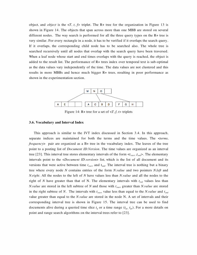
object, and object is the <T, t, f> triplet. The R+ tree for the organization in Figure 13 is shown in Figure 14. The objects that span across more than one MBB are stored on several different nodes. The way search is performed for all the three query types on the R+ tree is very similar. For every rectangle in a node, it has to be verified if it overlaps the search query. If it overlaps, the corresponding child node has to be searched also. The whole tree is searched recursively until all nodes that overlap with the search query have been traversed. When a leaf node whose start and end times overlaps with the query is reached, the object is added to the result list. The performance of R+ trees index over temporal text is sub-optimal as the data values vary independently of the time. The data values are not clustered and this results in more MBBs and hence much bigger R+ trees, resulting in poor performance as shown in the experimentation section.
Figure 14: R+ tree for a set of <T, f, t> triplets
3.6. Vocabulary and Interval Index This approach is similar to the IVT index discussed in Section 3.4. In this approach, separate indices are maintained for both the terms and the time values. The <terms, frequency> pair are organized as a B+ tree in the vocabulary index. The leaves of the tree point to a posting list of Document ID.Version. The time values are organized as an interval tree [23]. This interval tree stores elementary intervals of the form <tstart ,tend>. The elementary intervals point to the <Document ID.version> list, which is the list of all document and its versions that were active between time tstart and tend. The interval tree is nothing but a binary tree where every node N contains entries of the form N.value and two pointers N.left and N.right. All the nodes to the left of N have values less than N.value and all the nodes to the right of N have greater than that of N. The elementary intervals with tend values less than N.value are stored in the left subtree of N and those with tstart greater than N.value are stored in the right subtree of N. The intervals with tstart value less than equal to the N.value and tend value greater than equal to the N.value are stored in the node N. A set of intervals and their corresponding interval tree is shown in Figure 15. The interval tree can be used to find documents alive during a queried time slice tq or a time range (tqs, tqe). For a more details on point and range search algorithms on the interval trees refer to [23].

Figure 15: A set of intervals and their corresponding Interval tree
The procedure to perform all the three query types over the Vocabulary and Interval index is similar. In Figure 16, we show type III queries over the Vocabulary and the Interval Index.
Input: Term: Tq Time range: (ts, te) Procedure:
1 From the vocabulary index V, retrieve the list LV of document versions containing the term.
2 From the Interval index find the list of document versions DV alive between ts and te
3 Result = Join LV and DV on the document ID.version attribute.
Figure 16: Type III queries on the VINT index
4. EXPERIMENTAL EVALUATION We conducted a set of experiments on real world datasets to compare the solutions proposed in the previous section. Since all the solutions that we have proposed are exact techniques, they produce similar precision and recall values. For the purpose of comparison, we mainly focus on the index size and the retrieval times.

4.1. Data and system setup The techniques proposed in this paper were implemented using Java JDK 1.5. The experiments were run on a Xeon 3 GHz machine with 2GB of RAM. The numbers reported were averaged over 10 runs. All the data and the indices were stored using the Berkley DB open source database system [24]. For the data, we made use of revision histories from the English Wikipedia. The Wikipedia provides access to all the revision histories for a wiki article. There are some popular wiki articles that involve a lot of edits and modifications. There are also topics for which the edits are much less frequent and involve minor changes. We constructed two datasets from each of these two categories. Dataset 1 corresponded to 1000 versions of a wiki page for which there were frequent and major modifications spanning over a period of sixteen days. The average number of terms in this wiki page (excluding stop words) was 4341. Dataset 2 corresponded to 1000 versions of a wiki page for which the changes were minor and span over a year. The average term count for this wiki page was 2136. We built a query workload using a few keywords that were present in the wiki pages and also a randomly sampled time slice/range from within the duration spanned by two datasets. 4.2. Index sizes Our first set of experiments examine the index sizes of the techniques proposed in the previous section. The index size for both our datasets is summarized in Table 1.
Technique Index size for
Dataset 1 (in MB) Index size for
Dataset 2 (in MB)
Vocabulary Index 28.6 16.2
HVT Index 67.4 33.7
kd tree Index 46.8 31.5
IVT Index 72.3 36.7
R+ tree Index 65.7 21.6
VINT Index 60.1 20.6
Table 1: Index sizes for the two datasets
The vocabulary index had the least size for both the datasets as it only indexed the term values. The IVT index had the maximum size as both the time and the term information are both indexed independently. The R+ tree and the Vocabulary index approaches, which

associate time spans with the terms, are much smaller compared to the corresponding techniques that associate timestamps with terms. However, the size improvement was much more prominent for Dataset 2 compared to Dataset 1. This is because Dataset 2 had entries with minor modifications across versions. Thus, the terms have much longer time spans and the number of index entries is less. The growth in the index size for the VINT index is shown in Figure 14. For dataset 1, where the modifications between versions is much more prominent, the index size grows near exponentially. For the dataset 2, where modifications between versions are subtle, the growth in the index size is less than exponential.
Figure 14: Growth in index size for the VINT index
4.3. Query Execution time In order to compare the query execution times, we executed the three query types on our two datasets. The terms to search were randomly chosen from arbitrary versions of the document. For type II and III queries, a time slice/range was randomly generated from the duration spanned by the dataset. Figure 14 shows the search time for the type I query over the dataset. The performance was similar for the Vocabulary index, HVT index and the VIT index. Since, all these three techniques had separate indices for the vocabulary, the performance for the search involving only keywords was better compared to the performance of the other techniques. The VINT index had the best performance, as the size of the vocabulary index was the smallest for this technique.

Figure 14: Type I queries over the two datasets
The performance for type II and III queries is shown in Figure 15 and 16 respectively. For queries involving both time and the terms, the VI index slows down considerably as there is no index on the time attribute. The techniques that index both the time and the term values perform better than techniques that index only the terms. The query execution time is higher for type III queries compared to type II queries. Also, the KD tree and the R+ tree approaches were slower due to the large index sizes.
Figure 15: Type II queries over the two datasets

Figure 16: Type III queries over the two datasets
5. Conclusion
There is a growing importance for temporal text containment queries over versioned document sequences. The traditional information retrieval techniques, which provide efficient keyword based search, have to be extended to support search using both keywords and time. In order for the extensions to be practical, they need to be to be efficient with respect their space utilization and also their query execution times. In this work, we have examined various techniques for answering temporal text containment queries. We have also performed tests with two different datasets to closely examine the performance of the proposed techniques.

REFERENCES
1. Masanès, J., Web Archiving: Issues and Methods. Web Archiving, Springer, 2006: p. 1-53.
2. Song, S. and J. JaJa, A New Technique for Archiving Temporal Web Information, in
UMIACS Technical Report, University of Maryland Institute for Advanced Computer
Studies. 2008.
3. Zobel, J. and A. Moffat, Inverted Files for Text Search Engines. ACM Computing Surveys,
2006.
4. Zobel, J., A. Moffat, and K. Ramamohanarao, Inverted files versus signature files for text
indexing. ACM Transactions on Database Systems (TODS), 1998.
5. Anh, V.N. and A. Moffat, Inverted Index Compression Using Word-Aligned Binary Codes.
Information Retrieval, Kluwer Academic Publishers. 8: p. 151-166.
6. Deerwester, S., et al., Indexing by Latent Semantic Analysis. Journal of the American
Society for Information Science, 1990.
7. Papadimitriou, C., et al., Latent Semantic Indexing: A Probabilistic Analysis. Journal of
Computer and System Sciences– Elsevier, 2000.
8. Gaede and O. Gunther, Multidimensional Access Methods. ACM Computing Surveys, 1997.
9. Nievergelt, J., H. Hinterberger, and K.C. Sevcik, The Grid File: An Adaptable, Symmetric
Multi-Key File Structure. European Cooperation in informatics on Trends in information
Processing Systems, 1981.
10. Samet, H., The Quadtree and Related Hierarchical Data Structures. ACM Comput. Survey,
1984.
11. Robinson, J.T., The KDB-tree: a search structure for large multidimensional dynamic
indexes. Proceedings of the ACM SIGMOD international conference, 1981.
12. Guttman, A., R-Trees: A Dynamic Index Structure for Spatial Searching. ACM SIGMOD
International Conference on Management of Data, 1984.
13. Sellis, T., N. Roussopoulos, and C. Faloutsos, The R+-Tree: A dynamic index for multi-
dimensional objects. VLDB, 1987.
14. Date, C.J., H. Darwen, and N. Lorentzos, emporal Data & the Relational Model. Morgan
Kaufmann, 2002.
15. Snodgrass, R. and I. Ahn, A taxonomy of time databases. ACM SIGMOD international
conference on Management of data, 1985.
16. Salzberg, B. and V.J. Tsotras, Comparison of Access Methods for Time-Evolving Data.
ACM Comput. Survey, 1999. 31(2): p. 158-221.

17. Anick, P.G. and R.A. Flynn, Versioning a full-text information retrieval system. ACM
SIGIR Conference on Research and Development in Information Retrieval, 1992: p. 98-111.
18. Nørvåg, K., The design, implementation, and performance of the V2 temporal document
database system. Information & Software Technology, 2004. 46(9): p. 557-574.
19. Nørvåg, K., Space-Efficient Support for Temporal Text Indexing in a Document Archive
Context. Europen Conference on Digital Libraries, 2003.
20. Berberich, K., et al., FluxCapacitor: efficient time-travel text search. VLDB, 2007.
21. Gunadhi, H. and A. Segev, Efficient indexing methods for temporal relations. Transactions
on Knowledge and Data Engineering, 1993: p. 496-509.
22. Cole, R., et al., On the Dynamic Finger Conjecture for Splay Trees. SIAM Journal on
Computing, 2000: p. 1-43.
23. Cormen, T.H., et al., Introduction to Algorithms. MIT Press and McGraw-Hill, 2001.
24. BerkleyDB: Open Source database, www.oracle.com/technology/products/berkeley-
db/index.html