Independent Research Projects Tropical Marine Biology Class Summer 2014, La Paz, México

Western Washington University Universidad Autónoma de Baja California Sur

Title pp

Causes of balloonfish (Diodon holocanthus) stranding in the Gulf of California...............................................................................................................3

Genetic diversity comparison between the bottlenose dolphins Tursiops truncatus inhabiting the Gulf of California and those inhabiting the Atlantic Ocean…………………………………………………………...…..20

The ingestion of thermoplastic particulates by Coral reef fish Abudefduf troschelii ………………………………………….…………….29

Haplotype frequencies of green sea turtles (Chelonia mydas) Involved in a mass die-off even along the western coast of Baja California Sur, Mexico………………………………………………………………..54

Alarm response in Centrostephanus coronatus with increasing exposure to the predatory chemosensory cues of Heliaster kubiniji…………………………………………………....…………………..70

The effects of temperature diameter and arm number on the righting response of sea stars in the Gulf of California……………………………………90

A forensic, genetic analysis of the ribosomal ITS2 region in potential Shark samples taken from markets in the Baja Peninsula, México……………………….109

1

Summer 2014 Class

Students: Austin Abendroth Morgaine Angst Lesli Baker Denielle Beenken Gyovani Castañeda MacKenzie Gwinn Emily Hiatt Alexis Alejandro Jiménez Pérez Erin Matthews Felipe Antonio Muñoz Félix Mallory Ogburn Anna Pieri Sara Spitzer Jessica Stanley Kirsten Steinke Brittany Weiss Bethany Williams Faculty: Alejandro Acevedo-Gutiérrez Deborah Donovan Sergio Francisco Flores Ramírez Benjamin Miner

2

Causes of Balloonfish (Diodon holocanthus) stranding in the Gulf of California

Erin Matthews and Lesli Baker

Western Washington University 516 High Street Bellingham WA 98225

3

Abstract

Strandings of aquatic organisms can play an important role in the habitat

structure of beaches and intertidal regions by affecting population dynamics and species

composition within an area. Strandings can result from natural or anthropogenic

conditions. Although cetacean strandings are relatively well understood, researchers are

still sometimes unable to pinpoint the cause of a stranding. The causes and effects of

fish strandings are currently not well understood. We observed several Diodon

holocanthus populations at multiple beaches around La Paz, B.C.S Mexico, but an

uneven distribution of washed up D. holocanthus carcasses. We hypothesized that

healthy D. holocanthus individuals died as a result of stranding, as opposed to dying in

the water and washing up at a similar rate as other passive debris. We also predicted

that beach slope had an effect on the likelihood of a D. holocanthus stranding. We

hypothesized that fish body size would effect the likelihood of stranding. We recorded

the quantity of garbage and dead fish in transects at four beaches around La Paz, B.C.S

and then performed an experiment on live D. holocanthus. We exposed 26 individuals to

varying slope conditions and recorded strandings and body size. We found no

relationship between the slope of the beach and the susceptibility of D. holocanthus to

stranding. There was also no relationship between body size and likelihood of stranding.

We were unable to correlate dead fish with passive debris because no D. holocanthus

carcasses were found in our transects. We also made some observations while in the

field that implicates predator evasion behavior of D. holocanthus and large waves

created by boats as potential causes of D. holocanthus stranding.

4

Introduction

Strandings of aquatic organisms can play an important role in the habitat

structure of beaches and intertidal regions by affecting population dynamics within an

area (Nagrodski et al 2012, Hernández-Miranda 2010). They can offer an insight to the

anatomical structures of rare species, and provide information for detailed descriptions

that are otherwise not available due to the lifestyles of the organism (Pyenson 2010).

Occasionally, mass strandings of dozens, or hundreds, of individuals can occur within a

small area and can help provide estimates of population size and species composition

(Balcmob III, 2000, Hohn 2005, Pyenson 2010).

Strandings can result from sudden and unexpected changes in the surrounding

environment, due to natural or anthropogenic causes, like oil spills, hypoxic events,

disease, dramatic drops in water level, or predator evasion behaviors (Hernández-

Miranda 2010, Nagrodski et al. 2012). Strandings can also be triggered by anatomical

causes like malnutrition, secenense, disease or infection (Pyenson 2010). Additional

triggers may be large-scale changes in the patterns of climate, complexities of nearshore

geomorphology or geomagnetic interference of navigation, however this causes are not

exlusive and may transpire simultaneously (Pyenson 2010).

A stranding occurs when an aquatic organism is restricted to a habitat with

unsuitable water depth due to physical separation from a main body of water

(Nagrodski et al. 2012). In 2000, Balcomb and Claridge documented a stranding of two

beaked whales species that washed up on shore (Ziphius cavirostris and Mesoplodon

5

europaeus) in the Bahamas, and determined the cause was naval sonar. However the

causes of strandings are not always known. In 2005, NOAA documented a mass

stranding of three whales species (Globicephala macrorhynchus, Balaenoptera

acutorostrata and Kogia sima). Interestingly researchers were not able to identy a link

between all of the stranded individuals and a single anthropogenic or environmental

condition (Hohn 2005). Despite the fact that fish stranding may be an important issue,

especially when relating to anthropogenic environmental disruptions, there is currently

little knowledge related to strandings of fish. Research on this subject is important in

order to improve the accuracy when assessing threats to biodiversity or, if need be, to

establish effective mitigation strategies.

Despite the importance of strandings for intertidal and beach ecosystems, very

little is known about the causes or impacts of fish strandings. This study focused on

balloonfish (Diodon holocanthus), which is part of the spiny puffer fish family

Diodontidae. Diodontidae are common in tropical and temperate waters all over the

world and Diodon holocanthus are common in shallow waters in the Gulf of California

and along the Pacific Coast of Baja to Panama (Fujita et al. 1997, Humann and Deloach

2004). They are identifiable by a square shaped body with large straight spines that lie

flat (Wiktorowicz et al. 2007). Diodontidae are rigid-bodied, undulatory median and

paired-fin swimmers (UMPF), which means that they are generally smooth swimmers

with maneuverability and stability at slow speeds, but have little power output and slow

acceleration (Wiktorowicz et al. 2007, Blake et al. 2011, Korsmeyer et al. 2002).

Diodontidae are unique in their anti-predator defense of inflation behavior, called

6

puffing (Greenwood 2009). During a puffing event, the fish swallows water and uses its

stomach to inflate up to three times its relaxed state, which deters predators (Brainerd

1994). However, the anti-predator response of inflating also has its dangers. When a

pufferfish inflates, it’s ability to maneuver decreases. This increases their risk of drifting

into an undesirable environment, like shallow water along a beach and making them

more venerable to stranding then other species.

This led us to ask the questions: what causes fish to wash up on some beaches

and not others? Do D. holocanthus die in the water and wash up on the beach at similar

rates as other passive debris, such as plastic and glass? Or are D. holocanthus healthy

when they become stranded and die as a result?

We conducted our beach surveys and experiments at four sandy beaches near La

Paz, B.C.S, Mexico, that varied in beach slope, wave speed, and amount of debris

present. To see how the waves influenced the likelihood of a fish stranding, we placed

the fish in a holding area that spanned from the shallow water to some exposed sand.

We predicted that wave speed would positively correlate with number of dead fish. We

also expected beach gradient would be negatively correlated with number of fish

stranded in our natural experiment. We hypothesized stranded D. holocanthus died due

to stranding, as opposed to dying in the water and passively washing up on the shore

and therefore expected no relationship between amount of passive debris and number

of dead fish. Measurements for body size were also taken because we anticipated that

body size would affect the likelihood of a fish stranding in our natural experiment.

7

Methods

We observed many dead, and one dying, D. holocanthus at Balandra, a beach

near La Paz, BCS. Despite the presence of D. holocanthus at other nearby beaches, no

carcasses were observed. We were curious about the susceptibility of D. holocanthus to

stranding and what aspects of Balandra caused the increase in strandings seen. Our

study had two objectives. The first was to perform an experiment in which D.

holocanthus was placed in a testing corral where beach slope and wave speed mimicked

conditions hypothesized to be optimal for stranding to occur. The second was to

correlate stranded fish carcasses with beach slope, wave speed and abundance of non-

organic passive debris, such as plastic and glass. However, we found no dead fish during

our study.

For our study we selected beaches based on previous observations of fish

strandings. We sampled four beaches; Cantamar, Balandra, La Paz and Calerita, which

are all located near La Paz, Baja California Sur. Personal observations of dead D.

holocanthus at Balandra and La Paz designated them as possible stranding beaches. The

other two beaches were chosen because no strandings of D. holocanthus had been

previously noted. Cantamar was a small beach and was only sampled at one location.

Balandra was a large beach, which has four major coves, so we sampled two coves. We

eliminated the main beach because it is a very popular beach, which is routinely

8

cleaned. The cove on the left of the main cove was not accessible. At La Paz, we walked

along the main stretch of the beach, and numbered each beach with distinctive edges.

Out of the fifteen beaches, we chose one at random to test. At Calerita, the beach was

extremely long, so we used natural rock barriers to establish individual beaches to test,

and found two sandy beaches with different slopes.

At each beach, we documented trash and fish found within a 30 m by 2.05 m

transect. To locate a transect, we estimated the middle of the beach and randomly

choose a direction, left or right, and the starting distance from the middle. We placed

the meter tape along the edge of high tide mark, placed the of the transect along the

tape and went down beach from there. The trash we found was counted by item. Any

stranded or dead fish in the transect were noted; however no fish were found during

the study. After the transect was complete, we measured the slope of the beach and the

speed of the waves. To measure the slope, we used a straight PVC pipe, a measuring

tape and a level. To measure the wave speed, we dropped a lime into the water and

timed how long it took to become stuck on the beach.

To test our hypothesis that beach slope influenced the likelihood of a D.

holocanthus stranding we set up a testing corral which measured 4 meters by 1 meter

by 0.75 meters and was made from mesh and PVC piping at beaches with various slopes.

The testing corral was set up in the middle of the transect, with one end in the water

and the rest of the transect on the beach. We placed the end of the testing corral in the

water at a depth of 20 cm to 30 cm, to account for the change in height when waves

9

came in. The holding area measured 45 cm x 39 cm x 63 cm was set up before collection

and was used to house fish that had been tested to prevent recapture and retesting.

Once the testing corral was set up, we hand captured D. holocanthus by using a

small aquarium net and a mesh PVC net while snorkeling. This allowed a person to

corral the fish before scooping it into the net. The fish was then swam to shore, and

placed into a large bucket. Once the testing corral was double checked for holes, the fish

was introduced to the corral by submerging the bucket. Once the fish was securely in

the testing corral, a test began. If natural waves were not sufficient, a researcher

created artificial waves for one minute using the lid to the plastic tub, which was 45 cm

by 65 cm. If, at the end of a minute, the fish was not stranded, it was placed into the

holding area. If however, the fish became stranded within the time limit, for longer than

15 seconds, it was considered a stranding. We then returned the fish to the water. If the

fish did not strand for the full 15 seconds, and returned to the water by itself, then no

stranding was recorded. After each test, we took the fish’s length, width and height

measurements. If, before the test started, the D. holocanthus puffed, we allowed the

fish to return to its normal state before testing. If before testing started, a fish became

stranded within the testing corral due to natural waves, we timed the stranding to 15

seconds and returned the fish to the water. Also, if during the test, waves from a boat or

another artificial source besides the experimental waves, caused the fish to strike the

side of the enclosure, then we paused the test and removed the fish to ensure no injury.

10

Our data analysis included calculations of fish volume and two statistical tests.

For simplicity, we assumed a rectangular shape to estimate the volume of the D.

holocanthus, acknowledging that it is an over-approximation. Correlation and chi-

squared tests were run on five variables testing the strength of the relationships. We

analyzed our data using Pearsons’s product-moment correlation and Pearson’s Chi-

squared tests. We ran a correlation test on the number of strandings versus the angle of

the beach. We ran a chi-squared test on the size of the fish versus stranding occurrence.

We ran another chi-squared test on the number of times an individual fish puffed prior

to the experiment and whether or not they stranded. This was to ensure the stress

induced by capture was not affecting the likelihood of a stranding. All tests were run

using the statistical program R.

Results

Every location had at least two strandings occur, except for La Paz where the one

fish tested did not strand. 40% of fish stranded at Cantamar, 20% stranded at Balandra,

and 30% stranded at Calerita. Of the 26 total fish we tested, 7 stranded, and several

more fish struggled to swim against waves or even became stuck on the sand. Often

times, the fish that were stranded for less then 15 seconds were unable to free

themselves from the beach but they were pulled back into the deeper part of the testing

corral by a large wave. Those that stranded for less then 15 seconds were not recorded

as a stranding. We also observed a stranding outside of our experiment while pursuing a

11

D. holocanthus. One individual swam into very shallow water while attempting to evade

capture, was stranded by a natural wave and had to be removed from the beach and

placed into our holding area.

Beach slope was greatest at the first sandy cove at Balandra, with an angle of

12.33 degrees. The beach with the lowest gradient was the second beach at Calerita,

with an angle of 3.52 degrees. The other angles ranged from 6.09 to 9.28 degrees. The

highest number of strandings occurred at the transect with the lowest angle, however

we found no significant correlation between the number of fish that became stranded

and the slope of the beach (Figure 1, r=0.464, p=0.0354, df=4).

The volumes of the fish ranged from 14.9 cm3 to 39.1 cm3, however there was no

relationship between the volume of a fish and stranding. 13 fish puffed a total of 26,

though there was no relationship between the number of times a fish puffed and the

likelihood of a stranding occurring. The natural wave speed ranged from 30 seconds per

meter to 122 seconds per meter. However, we were unable to test the relationship

between wave speed and number of fish stranded because the wave speed of the

artificial waves was never measured.

Discussion

Contrary to our hypothesis, our data suggests that beach slope has no effect on

strandings of Diodon holocanthus. We also predicted there would be a relationship

12

between fish volume and likelihood of a stranding but we found no significant

relationship. Although our methods of capturing and transporting D. holocanthus did

cause stress, we found no relationship between the number of puffing events and the

likelihood of them being stranded. In other studies, the water level played a part in the

strandings of live fish, however currently there is no evidence that wave action, or water

level, effects D. holocanthus standings (Nagrodski 2012). Unfortunately, due to the lack

of data on garbage and dead fish we were not able to determine if the D. holocanthus

were washing up dead, and passively along with garbage, or whether they washed up

alive and then died.

We made several important observations during data collection that warrants

provide alternative explanations besides beach morphology. During one trial a D.

holocanthus was in the testing corral on a calm day, the individual the beach was struck

by waves created by a large boat. These boat waves were powerful enough to cause

unnecessary stress and the experimental was halted. Had we left the fish in the testing

corral, it was likely the fish would have been stranded and possibly injured. This leads to

the question about whether unexpected boat waves are causing strandings, and that

beach morphology does not play a role. We also observed a stranding while a D.

holocanthus was attempting to evade our capture. This individual swam into shallow

water and was stranded by a naturally occurring wave. The predator evasion technique

this fish displayed may indicate a behavioral aspect to fish strandings. Based on these

observations, boat waves and predator evasion behaviors may be two of the causes of

D. holocanthus strandings.

13

Despite not finding dead fish within our transects, there were carcasses on the

beach. A future study including larger transects and necropsies of freshly stranded D.

holocanthus might be able to address the question as to whether the fish are healthy

when washing up on the beach or if they are dying or dead. Though we tried limiting

confounding variables, most beaches we tested were cleaned on a regular basis, thus

eliminating the possibility of finding carcasses. Also, testing a wider range of body sizes

might draw out a correlation between size and stranding. There is still much more

investigation needed regarding the causes of fish stranding.

14

References:

Balcomb, K. C., and D. E. Claridge. 2001. A mass stranding of cetaceans caused by naval

sonar in the Bahamas. Bahamas Journal of Science p. 1 – 12.

Blake, R. W., and K. H. S. Chan. 2011. Biomechanics of swimming in the pufferfish

Diodon holocanthus: propulsive momentum enhancement is an adaption for

thrust production in an undulatory median and paired-fin swimmer. Journal of

Fish Biology 79: 1774-1794.

Brainerd, E. L. 1994. Pufferflish Inflation: Functional morphology of postcranial

structures in Diodon holocanthus (Tetraodontiformes). Journal of Morphology

220: 243-261.

Greenwood, A. K., C. L. Peichel and S. J. Zottoli. 2009. Distinct startle responses are

associated with neuroanatomical differences in pufferfish. The Journal of

Experimental Biology 213:613-620.

Hernández-Miranda, E., R. A. Quiñones, G. Aedo, A. Valenzuela, N. Mermoud, C. Román

and F. Yañez. 2010. A major fish stranding caused by a natural hypoxic event in a

shallow bay of the eastern South Pacific Ocean. Journal of Fish Biology 76: 1543-

1564.

15

Hohn, A. A., D. S. Rotstein, C. A. Harms, and B. L. Southall. 2005. Multispecies Mass

Stranding of Pilot Whales (Globicephala macrorhynchus), Minke Whale

(Balaenoptera acutorostrata), and Dwarf Sperm Whales (Kogia sima) in North

Caroline on 15-16 January 2005. NOAA Techincal Memorandum NMFS-SEFSC-537

p: 1 – 230.

Humann, P., and N. Deloach. 2004. Reef Fish Identification Baja to Panama. First Edition.

New World Publications.

Fujita, T., W. Hamaura, A. Takemura and K. Takano. 1997. Histological observations of

annual reproductive cycle and tidal spawning rhythm in the female porcupine

fish. Diodon holocanthus. Fisheries Science 63: 715-720.

Korsmeyer, K. E., J. F. Steffensen and J. Herskin. 2002. Energetics of median and paired

fin swimming, body and caudal fin swimming, and gait transition in parrotfish

(Scarus schlegeli) and triggerfish (Rhinecanthus aculeatus). The Journal of

Experimental Biology 205: 1253-1263.

Nagelkerken, I., M. Dorenbosch, W. C. E. P. Verberk, E. Cocheret de la Moriniere, and G.

van der Velde. 2000. Day-night shifts of fishes between shallow-water biotopes

of a Caribbean bay, with emphasis on the nocturnal feeding of Haemulidae and

Lutjanidae. Marine Ecology Progress Series 194: 55-64.

16

Nagrodski, A., G. D. Raby, C. T. Hasler, M. K. Taylor and S. J. Cooke. 2012. Fish stranding

in freshwater systems: Sources, consequences and mitigation. Journal of

Environmental Management 103: 133-141.

Pyenson, N. D. 2010. Carcasses on the coastline: measuring the ecological fidelity of the

cetacean stranding record in the eastern North Pacific Ocean. Paleobiology 36:

453-480.

Wiktorowicz, A. M., D. V. Lauritzen, and M. S. Gordon. 2006. Powered control

mechanisms contributing to dynamically stable swimming in porcupine puffers

(Teleostei: Diodon holocanthus). Exp Fluids 43: 725-735.

17

Figure Caption

Fig 1. A correlation between angle of beach slope and the number of strandings per

beach transect.

18

Figure 1.

19

Gyovani Castaneda

Thursday, July 31st 2014

Tropical Marine Biology 497

Genetic diversity comparison between the bottlenose dolphins Tursiops truncatus inhabiting the Gulf of California and those inhabiting the Atlantic Ocean

Group members: Gyovani Castaneda

Universidad Autónoma de Baja California Sur, Carretera al Sur Km 5.5, La Paz, México, CP 23080

Abstract

Data obtained from Natoli et al, 2004 and Iris-Segura et al, 2006 was re-analyzed

in order to compare the different populations of bottlenose dolphins belonging to

the type Tursiops spp. Found within the gulf of California, the eastern north

Pacific (ENP), the north western Atlantic pelTagic (WNAP), north western Atlantic

coast (NWAC), south Africa (SA) and Bahamas (BAH), the mtDNA sequences

were processed with CLUSTALX, a multiple sequence alignment (MSA) software

that enabled us to compare the sequences yet with another software,

ARLEQUIN. Results showed the molecular divergence (Fst = 0.18) along with

their significance (P) values and also the migration index within the populations

(M). The results obtained supported our hypotheses that had been formulated

prior to the experiment, which stated that genetic divergence between bottlenose

dolphin populations would increase with geographic distance and significant

geographic barriers (i.e. continents). Our discussion focuses on how is it that

genetic differentiation is low within bottlenose dolphins within the gulf and high

compared to the populations from other parts of the world according to

geographical barriers. Although dolphins are highly mobile individuals, there are

ecotypes that will be isolated from other populations due to extensive risk when it

comes to migration activity.

Introduction

Bottlenose dolphins are known to inhabit both hemispheres, ranging from cold-

temperate to tropical waters. Although geographically close to each other,

20

differentiation among morphotypes is highly noticed. Ecological and

environmental pressures affect the evolutional trajectories of morphological traits

within bottlenose dolphin populations, thus promoting differentiation of ecotypes

(diet, morphology and spatial distribution) among these groups. It is believed that

founder events followed by parallel adaptations marked the distinct ecological

niches with their “signature” and ever since different groups have struggled

against natural selection and thus developed maintained specific morphotypes

that fit into that specific ecology (Louis et al., 2014). The pressure for

reproduction in dolphins in high, due to the fact that females only become fertile

once every four years, making them a highly precious resource for males.

Interbreeding does take place within populations to maintain habitat

specialization, but this is also double edged sword, since a lot of inbreeding could

cause a genetic disorder within populations. Groups of males are formed in order

to venture into different areas and look for females in order to spread their genes,

thus homogenizing populations and making them more similar. Offshore male

bottlenose dolphins are thought to be the primary diversity vectors when it comes

to species gene flow, since males tend to disperse as their reproductive success

is constrained by access to mates (Emlen & Oring, 1977; Greenwood, 1980),

these males can travel long distances in order to breed with coastal populations

from different locations. It is well documented that offshore bottlenose dolphin

populations are more genetically diverse than costal ones, thus becoming the

major influence when it comes to homogenizing worldwide populations. In the

Pacific, mitochondrial DNA (mtDNA) genetic differentiation between coastal and

pelagic bottlenose dolphins is significant, but there is no complete lineage sorting

(Segura et al. 2006). Tezanos-Pinto et al. (2009) suggested that ecotype

differentiation in the NWA may not be representative of genetic structuring of

bottlenose dolphins worldwide.

Materials & Methods

Data-mining of the results found in two literature articles from Iris-Segura et al.

(2006) and Natoli et al. (2004), which show the mtDNA sequences they obtained

21

through the sampling of different bottlenose dolphins. The 83 skin tissue samples

from Iris’ paper were obtained at different latitudinal locations throughout the Gulf

of California: in the northern region they sampled at the Rio Colorado delta, south

of the Midriff islands, off Bahia Concepcion, around Loreto, around San Jose and

Espiritu Santo islands, in Bahia de La Paz and the southern GC. In Natoli’s

paper, the 269 Tursiops samples used were obtained from seven geographic

regions, but we only included five of them, leaving out the data they obtained

from the Mediterranean Sea and Gulf of Mexico. Samples from SA were

collected from a coastal population described as T.Aduncus, while all others

samples were from individuals described as T. truncates. Samples from WNAC

and WNAP are from Hoelzel et al. (1988). ENP samples were from California

(strandings and probably coastal habitat, but this is not known). Both sampling

collections differ in that, in Natoli’s investigation they got their samples from

stranding and byfishing individuals, whilst samples obtained in Iris’ investigation

were acquired with the use of a crossbow and darts with steel collector tips. Both

authors preserved their samples in a saline buffer (saturated NaCl, 20% DMSO)

but only in the Iris’ paper they mention 250 mM EDTA. Both authors extracted

the DNA from their samples, differing in their methods, Natoli used a standard

phenol/chloroform extraction method and Iris used proteinase K digestion, LiCl

protein salting-out organic extraction, and ethanol precipitation (Aljanabi and

Martinez, 1997) and with the DNA-easy tissue kit. Authors used different primers

for amplifying their DNA, Iris used the L15812 (Escorza-Trevino et al., 2005) (50

CCT CCC TAA GAC TCA AGG 30) and H16343 (Rosel et al., 1994) (50 CCT

GAA GTA AGA ACC AGA TG 30) in 25 lL PCR reactions (150 lM each dNTP,

1.5 mM MgCl2, 10mM Tris, 50 mM KCl, 0.3 lM each primer and 0.5 U Taq

polymerase). Natoli used Primers KWM1b, KWM2a, KWM2b, KWM9b and

KWM12a that derived from O.orca (Hoelzel et al., 1998b), EV37Mn from

Megaptera novaengliae (Valsecchi & Amos, 1996), TexVet7 and D08 from

T.truncatus (Shinohara et al., 1997; Rooney et al., 1999). Each author then went

through the process of PCR cyclying with different time lengths and annealing

temperatures and consequently obtained the allele sizes with biosystem and

22

gene analyzer software. Microsatellite loci were used to screen samples from

different geographical areas as well as different software for multiple sequence

alignments. Natoli used FSTAT 2.9.3 (Goudet, 2001) to calculate allelic richness

controls for variation in sample size by a refraction method and Iris used

MODELTEST 3.6 to determine the optimal model of nucleotide evolution, which

was employed in the rest of molecular analyses. Iris also used ARLEQUIN to

compute genetic diversity indices and phylogenetic relationships among mtDNA

haplotypes were reconstructed with the program PAUP* 4.0b10.

Our methods consisted in performing the MSA with the data obtained from both

authors’ results and cutting the strands that were not able to aligned, “leftover

strands”. Then the strands were copied to a word document, so they could be

arranged in a FASTA format previous to be introduced into the ARLEQUIN

software for genetic differentiation testing. Population names for the groups of

sequences were assigned separated into four divisions: 1: GN, 2: GI, GC, GS,

SIN, BB and ENP; 3: WNAP, WNAC and BAH; 4: sAFR. In the AMOVA section,

standard AMOVA computations (haplotypic format) option was selected, with a

No. of 1000 permutations and conventional F-statistics were used. In the

Population structure section, “Compute pairwise FST was selected and for the

genetic distances, the Slatkins and Reynolds distances were selected. Compute

pairwise differences (pi) was also selected as a population comparison setting

with a number of 1000 permutations and a significance level of 0.05, and then

the option for using conventional F-statistics was selected as well. In the

population differentiation section, Exact test of population differentiation was

selected, with a 1000 steps in the Markov chain as well for No. of

dememorization steps. The program was set to run and the results sheet was

shown. Once results were obtained, matrixes obtained from FST and M values

(see table 1 and 2) were analyzed and significance values marked thick

(denoted), the highest and lowest values for both Gulf of California and rest of

the world were marked with different colors. Graphs were made in excel to show

23

the correlation between both genetic divergence and migration indexes with

distance (see fig 1 and 2). Results Computing conventional F-Statistics from haplotype frequencies. There is a pattern observed between the different groups, when comparing the Gulf populations within each other and then comparing them with the other populations farther away. Below the line that separates the gulf populations from the rest, FST values are significant different between gulf populations and the rest of the world (P<0.05, t= 2.82, D.F=8). N.Gulf Gulf I. C. Gulf S.Gulf Sinaloa B.B. E.N.P. W.N.A.P. W.N.A.C. S.AFR Bahamas N.Gulf * Gulf I. 0.11240 * C.Gulf 0.09409 0.05849 * S.Gulf 0.09485 0.06024 0.05038 * Sinaloa 0.16847 0.13929 0.11442 0.11501 * B.B. 0.08219 0.03648 0.02776 0.02985 0.10762 * E.N.P. 0.35812 0.37223 0.29146 0.28939 0.42609 0.34375 * W.N.A.P. 0.13872 0.10694 0.08955 0.09044 0.16351 0.07652 0.35354 * W.N.A.C. 0.36543 0.39655 0.29377 0.28323 0.43130 0.37687 0.64455 0.36282 * S.Afr. 0.19032 0.16757 0.13672 0.13634 0.22297 0.13813 0.43180 0.18576 0.43004 * Bahamas 0.27739 0.27974 0.21571 0.21304 0.33016 0.25311 0.60396 0.27321 0.53673 0.34081 *

Table 1. Haplotypic tree of the 11 different populations sampled, horizontal line separates Gulf of California populations from Pacific and Atlantic populations. Data marked with yellow marker represent the highest values whilst data marked with blue marker represent the lowest. Significant values are thick black marked. The matrix for the migration indexes correlates with the FST values from Table 1. The lower the FST value between two populations, the higher the migration index between two populations. Black line delimits Gulf of Calfornia populations and Atlantic Ocean populations. M values for Gulf of California and Atlantic Ocean are significantly different (P<0.05, t=-3.5, D.F.=8). ------------------------------------------------------------------ Matrix of M values (M=Nm for haploid data, M=2Nm for diploid data) ------------------------------------------------------------------ N.Gulf Gulf I. C. Gulf S.Gulf Sinaloa B.B. E.N.P. W.N.AP. W.N.A.C. S.Afr. N.Gulf Gulf I. 3.94852 C.Gulf 4.81419 8.04793 S.Gulf 4.77137 7.80065 9.42536 Sinaloa 2.46795 3.08959 3.86991 3.84743 B.B. 5.58332 13.20755 17.50989 16.24938 4.14615 E.N.P. 0.89618 0.84324 1.21549 1.22774 0.67347 0.95455 W.N.A.P. 3.10448 4.17563 5.08352 5.02831 2.55799 6.03465 0.91425 W.N.A.C. 0.86824 0.76087 1.20201 1.26536 0.65930 0.82673 0.27574 0.87808 S.Afr. 2.12710 2.48379 3.15722 3.16723 1.74243 3.11985 0.65794 2.19158 0.66267 Bahamas 1.28738 1.81798 1.84693 1.01441 1.47541 0.32787 1.33007 0.43157 0.96711

Table 2. Matrix value of migration indexes showing how much migratory activity there is between two populations. Data marked with yellow marker represent the highest values whilst data marked with blue marker represent the lowest. Black line delimits Pacific populations and Atlantic populations. Significant values are thick black marked.

The highest value that the genetic differentiation test showed between populations that within the Gulf of California is 0.16847, which is significant P<0.0001 between the Northern Gulf and Sinaloa and the lowest being 0.05038 with a significance P value of <0.001 between the Central Gulf and Southern

24

Gulf. As for the Gulf of California being compared to worldwide populations, the highest value observed is 0.64455 between the W.N.A.C. and E.N.P. with a significance of P<0.001 whilst the lowest value observed is found between W.N.A.P. and C. Gulf with a significance value of P<0.001.

Fig. 1- Northern Gulf populations being compared with different populations (Pacific and Atlantic). Trend line is positive, suggesting that there is a positive correlation between both distance and geographical with genetic divergence.

302 km582 km

716 km

812 km

1356 km

1358

3647 km

4566 km

4962 km

13,689 km

0

0.05

0.1

0.15

0.2

0.25

0.3

0.35

0.4Northern Gulf compared with Gulf populations

Gulf I. C.Gulf Sin S.Gulf E.N .P. B.B. W.N.A.C. Bah W.N.A.P. S.Afr

FSTs

25

Fig. 2 - Northern Gulf migration indexes compared to other populations. There is a negative correlation of number of migrations and distance, the farther away 2 populations are, the less number of migrations there will be.

Discussion

The northern Gulf was taken as the main reference when comparing the FSTs and M

values with one another because that is where Iris-Segura et al. (2006) got their most

samples from. Geographical distance and barriers do affect the genetic divergence

between populations of bottlenose dolphins. There had been thoughts about transient

pods of bottlenose dolphins that migrate from coast to coast, often breeding with other

populations already settled in that area, in the long run this could’ve had an enormous

gene flow. The fact that some FSTs values are higher than others and there is less

distance between those two populations might be due to the fact that populations overlap

when because of excursions in response to prey movements, such as those from

epipelagic fishes that are known to seek refuge in Bahia de La Paz (Arreola and

Gonzales, 1997). This, however does not mean that will be genetic gene flow between

populations, philopatry may help preserve gene differentiation, more likely in marine

mammals (Dizon et al., 1992). Specialized coastal populations are likely to only roam

around defined areas, unlike offshore ones that travel in big pods and are usually unstable

when it comes to area coverage. In both the W.N.A.C. and the G.C. genetic diversity was

302 km

582 km

716 km

812 km

1356 km

1358 km

3647 km4566 km

4962 km

13,689 km

0

1

2

3

4

5

6Northern Gulf migration index compared to other populations

Gulf I. C.Gulf Sin S.Gulf E.N.P. B.B. W.N.A.C. Bah W.N.A.P. S.Afr

#Haploids

26

higher in coastal populations that offshore populations, one of the reasons that could

explain this may be the fact that offshore populations travel in bigger pods and so they

maintain higher levels of gene diversity. The ecological conditions in the Gulf of

California favor the reproductive isolation between ecotypes within it, making it harder

for other pelagic populations traveling inside the gulf to breed with local individuals.

However, the Gulf of California has a relatively narrow continental shelf and a complex

topography of the, that could make it easier for pelagic pods to come and associate with

the coast line, where deep habitats can be found close to shore (e.g. deep basins), making

it harder to identify coastal boundaries.

The W.N.A.P. populations showed low divergence comparing them to the central G.C. so

there could be pelagic populations interacting with coastal ones and somehow reaching as

far as going around a whole continent. Some coastal groups are resident but movements

were reported between Corsica and France (360 km) (Gnone et al. 2011), indicating that

individuals crossed pelagic waters. Since female bottlenose dolphins’ reproductive

success depends mostly on food resources it is most important for them to be familiarized

with their natal habitat and won’t have to worry about dispersing (philopatry), unlike

males whose reproductive success depends on finding fertile females and have to spread

around large areas in order to find them. These processes could lead to large dispersal

behaviors among males and thus maintaining genetic diversity at a large scale between

coastal and offshore populations (Louis et al. 2014).

References

Aljanabi, S.M., Martınez, I., 1997. Universal and rapid salt-extraction of high quality genomic DNA for PCR-based techniques. Nucl. Acids Res. 22, 4692–4693. Angier, Natalie. 1988. Dolphin Courtship: brutal, cunning and complex. The New York Times.

Arreola, L., González, E., 1997. Composición, abundancia y distribución de larvas de peces en la Ensenada de La Paz, B.C.S. México. Revista de Investigación Científica Serie Ciencias Marinas UABCS 7, 23–39. Emlen ST, Oring LW (1977) Ecology, sexual selection and the evolution of mating systems. Science, 197, 215–223.

27

Goudet, J. 2001. FSTAT, A Program to Estimate and Test Gene Diversities and Fixation Indices (Version 2.9.3). Available at http://www.unil.ch/izea/softwares/fstat.html. Greenwood PJ (1980) Mating systems, philopatry and dispersal in birds and mammals. Animal Behaviour, 28, 1140–1162.

Hoelzel, A.R. 1998a. Genetic structure of cetacean populations in sympatry, parapatry and mixed assemblages: implications for conservation policy. J. Hered. 89: 451–458. Louis, M., Viricel, A., Lucas, T., Peltier, H. Alfonsi, E., Berrow, S., Brownlow, A., Covelo, P., Dabin, W., Penrose, R., Silva, M., Guinet, C., Bouhet-Simon, B. 2014. Habitat-driven population structure of bottlenose dolphins, Tursiops truncatus, in the North-East Atlantic. John Wiley & Sons Ltd. Molecular Ecology 23, 857-874. doi 10.1111/mec.12653. Shinohara, M., Domingo-Roura, X. & Takenaka, O. 1997. Microsatellite in the bottlenose dolphin Tursiops truncatus. Mol. Ecol. 6: 695–696. Tezanos-Pinto G, Baker CS, Russell K et al. (2009) A worldwide perspective on the population structure and genetic diversity of bottlenose dolphins (Tursiops truncatus) in New Zealand. Journal of Heredity, 100, 11–24. Valsecchi, E. & Amos, B. 1996. Microsatellite markers for the study of cetacean populations. Mol. Ecol. 5: 151–156.

28

The ingestion of thermoplastic particulates by coral reef fish Abudefduf troschelii

1ANNA PIERI, 1KIRSTEN STEINKE, 2FELIPE ANTONIO MUÑOZ-FELIX

1Western Washington University, 516 High Street Bellingham WA, 98225 USA

2Universidad Autónoma de Baja California Sur, Carretera al Sur Km 5.5, La Paz,

México, CP 23080

29

Abstract

Approximately six and a half million tons of plastic debris ends up in our oceans

annually negatively impacting over 267 species of marine organisms. The most common

of this debris found is high and low density thermoplastics. Many large mammals and

birds have been known to ingest plastic, but little information has been gathered on

ingestion by planktivorous fish. In this study we looked at the species Abudefduf

troschelii: a small pelagic coral reef fish that feeds on zooplankton and other

microorganisms. Our goal was to see if micro-plastics would be ingested by this species.

We hypothesized that the life-stage of the fish would affect the amount of plastics

consumed and that there would be a preference in clear, white, and green plastics

associated with their planktonic or micro-algal food sources. We tested in the field the

ingestion of two high-density plastics (HDP): polypropylene and polyvinyl chloride

(PVC) as well as two low-density plastics (LDP): polystyrene and polyethylene. Both

juveniles and adults ingested all four types of plastics, but juveniles consumed more

plastic than adults. This was due to the excessive amount of polystyrene consumed by the

juveniles. A preference for micro-plastics that were pink, red, and white was observed.

These colored plastics could have been confused as certain foods in their diet like

mesocrustaceans and polychaetes. We concluded that the ingestion of micro-plastics by

A. troschelii is a result of their confusion between the plastics and the species they

typically consume. The plastics that were used in this experiment are known to absorb

and transmit harmful chemicals. The fact that these lower trophic-level fish consumed

them poses a threat to the entire food web by being transferred up the trophic pyramid.

30

Introduction

Plastic pollution is a serious environmental problem in the marine environment,

and has only recently been recognized by the scientific and global community (Derraik,

2002). Even in the most remote regions of the world’s oceans, plastic pollution is

becoming a rising problem (Morris, 1980). Due to the photo-degradation of plastic

objects on surface waters, most plastic particulates persist in the ocean as micro-plastics

ranging from 1-5mm in diameter (Cozar, et al. 2014). Other forms of plastic breakdown

consist of embrittlement and fragmentation by wave action (Cozar, et al. 2014). This

material has become the fastest growing segment of the US municipal waste stream

(Moore, 2008). Marine litter is now 60–80% plastic in most regions, but can be 90–95%

in other parts of the ocean (Moore, 2008). Currently, there are 265 million tons of plastic

produced annually, where it is estimated that 6.5 million tons of that plastic waste ends

up in the ocean (Hammer et al., 2012). Oceanic plastic waste input is much higher than

the quantitative output observed in the water column (Cozar et al., 2014). There are four

reasons as to why this might occur: nano-fragmentation, bio-fouling, shore deposition

and predation of plastics can all play a role in elimination of plastic from the ocean

(Cozar et al., 2014). While the ingestion of macro-plastic debris by turtles, seabirds, and

large marine mammals has been a common area of study for many researchers, the

research on micro-plastics ingested by lower trophic level and planktivorous fish has not

been examined as thoroughly (Boeger, et al., 2010).

As the levels of micro-plastics increase due to the breakdown of macro-plastics

(Ivar do Sul and Costa, 2014), researchers are starting to focus on the ability of plastic to

absorb and transport toxins to aquatic organisms via ingestion (Moore, 2008). The

31

general concept understood thus far is that plastic particulates present in the marine

environment can carry chemicals of a very small molecular size (MW<1000 g/mol)

(Teuten et al., 2009). If ingested, these chemicals can penetrate through the cell

membrane and interact with biologically important molecules, which can disrupt the

endocrine systems of marine organisms (Teuten et al., 2009). The knowledge on hazards

correlated with the composite mixture of plastic and accumulated toxins is not thoroughly

developed and is in desperate need of research (Rochman, et al., 2013a).

Our intention was to further the understanding of plastic ingestion by fish that

might feed on micro-plastics, such as Abudefduf troschelii. Juvenile A. troschelii form

feeding aggregations of ten to thirty individuals and feed on planktonic organisms

swimming in the mid-water column or just under the surface (Hobson, 1965). Some

studies reveal diet changes during the growth of damselfishes, although throughout their

lifetime they continue to feed on zooplankton (Hobson, 2005). As adults, they are seen

over rocky bottoms where the majority of their food consists of material taken from the

rock surfaces such as algae, small crustaceans, anthozoans, copepods, tunicates,

polychaetes, and fish eggs (Hobson, 1965; Moreno-Sanchez, 2009). There is not much

information on this size interval, corresponding to that of zooplankton, and is due to the

fact that these data are hard to track (Cozar, et al. 2014).

Because zooplanktivorous fish exemplify a large portion of the trophic pyramid

within the ocean, and it is known that accidental ingestion of plastic occurs during their

feeding activity, this provides a stimuli for further investigation on the effects of plastic

toxins in a species and their predators (Cozar, et al. 2014). Higher trophic level predators

prey upon these smaller pelagic fish and once ingested, the toxins absorbed from the

32

plastics can be transferred through the predator’s body and eventually make their way up

the food chain. (Cozar et al., 2014). “The reported incidence of plastic in stomachs of

epipelagic zooplanktivorous fish ranges from 1 to 29%, and in stomachs of small

mesopelagic fish from 9 to 35%” (Cozar et al., 2014). Our study aimed to find out if

plastic particulates are being consumed by zooplanktivorous fish. The results from this

study could be used in further research to discover if and how these toxins proliferate

through the food web.

The question we asked was: does Abudefduf troschelii ingest planktonic-sized

thermoplastics, and if so, is one type of thermoplastic more commonly ingested than

others? The A. troshelii that were used for this experiment were collected off the shore of

Hotel Cantamar in Pichilingue Bay, B.C.S., Mexico and were exposed to polyethylene,

polypropylene, polystyrene, and polyvinyl chloride. We chose these plastics because they

are known to be associated with toxins that can proliferate through ecosystems if broken

down or unmonitored (Rochman, et al. 2013a). We hypothesized that A. troschelii would

ingest planktonic-sized thermoplastics because they would confuse floating micro-

plastics with their food source. Our second hypothesis was that juveniles would ingest

more plastic than adults because juveniles consume more food particles due to their

smaller body size and faster metabolic rate. We also hypothesized that A. troschelii was

more likely to ingest plastics that are similar in color to their planktonic or micro-algal

food source. Our predictions were that clear or translucent particles would be ingested the

most, followed by green and white, and that there would be preference for these colors

over the other colors tested (red, pink, black, yellow, brown, blue, and orange). Other

studies have shown that the ingestion of plastics similar in color to those of the area’s

33

plankton could be simultaneously consumed with the primary food sources of surface

feeding fish (Boeger, et.al. 2010).

Methods

In order to induce the least amount of stress in our fish, we decided to do field

tests by creating submersible cages that were anchored close to their collection site.

Cages were constructed out of PVC piping, duck tape, zip ties, and gardening mesh. We

attached plastic bottles to the cages for floatation to allow better observation of the fish

while recording data. The 3 adult submergible cages were made into 1 x 1 x 1 meter

enclosures and the 3 juvenile cages were 0.7 x 0.7 x 1 meters.

We captured our fish at night in the rocky intertidal area off the shore of Hotel

Cantamar in Pichilingue Bay, B.C.S., Mexico. We used dive lights and handheld nets to

capture fish. Once we had collected forty-five individuals, we divided them into their

respected cage. We had five adults (~15-25 cm in length) in each designated adult cage

and ten juveniles (~7-15 cm in length) in each designated juvenile cage where we kept

them contained until experimentation.

After a day of acclimation, we started our first trial. This consisted of a morning

and afternoon plastic feeding session where we tested one HDP and one LDP during each

session. We repeated this for three days switching the types of plastics fed in the morning

and the evening. Each trial consisted of two sessions where each session tested one high-

density and one low-density plastic on all six submersible cages. We offered the fish

plastic each day during their natural feeding times: 11:00 a.m. and 4:00 p.m.

34

To determine whether juveniles and adults consumed or preferred different types

of microplastics, we manually fed two low-density plastics (LDP): polyethylene and

polystyrene as well as two high-density plastics (HDP): polypropylene and polyvinyl

chloride to the test subjects over a three day timespan. Polypropylene (HDP) was

prepared by cutting up varying colors of plastic bottle caps (red, blue, and orange) and for

the white polypropylene, yogurt containers were cut up and used. The polyethylene

(LDP) samples were assembled from tiny pieces of plastic bags colored pink, brown,

black, green, blue, yellow, clear and white. Polystyrene (LDP) was pulled apart from a

Styrofoam block and polyvinyl chloride (HDP) was cut with a PVC cutter. There was

only one color option for polystyrene and polyvinyl chloride, which was white.

During feeding, we released eighty plastic particulates into each cage and

observed the behavior of the fish for five minutes. For the plastics that had multiple

colors, the eighty pieces were split up evenly between particulates (i.e. polyethylene had

ten pieces of each colored plastic and polypropylene had twenty pieces of each colored

plastic) and all of the colors were released at the same time. The high-density PVC would

sink, so these samples would be dropped from the top of the submersible cage. The low-

density polyethylene pieces were small squares of plastic bag that would slowly sink, but

would often times float out of the cage if we released them from the top. To ensure the

particulates were getting through the testing site we opened the bag in the middle half of

the cage and pushed it through horizontally by swishing the water towards the cage. The

polystyrene and polypropylene floated to the top so it was released at the bottom of the

cage. After the distribution of plastic at each cage, we collected the floating plastic with

35

handheld nets and discard the remnants in a waste container. We recorded the number of

ingestions of plastic particulates for each trial using underwater recording tablets.

Statistical analyses were done using R (R Development Care Team, 2014) where

ANOVA tests were used to test for differences among fish life-stage, plastic color and

type. A blocked two factor ANOVA was performed to test whether there was a difference

in type of plastic ingested, a difference in life stage of the test subjects, and whether or

not there was a relationship between the life stage of the fish and the amount of plastic

ingested per fish per cage per trial. Another blocked two factor ANOVA was performed

and tested the variance within color preference of plastic and the relationship between

plastic color and type of plastic. The last test we ran was a blocked one factor ANOVA to

see if there were differences in the amount of plastic ingested for each trial.

Ethical Statement

The capture of individuals was performed as cautiously as possible. After we

caught the fish, we left them in the submersible cages for one day to acclimate.

Throughout the length of the experiment we made sure our test subjects were in good

condition prior to running our tests. We would have stopped the experiment immediately

if the health of the fish seemed to be effected, however this was never an issue. Following

the plastic ingestion trials, we recollected all the plastics from the testing area. After all of

our trials, we released the fish where we had collected them.

36

Results

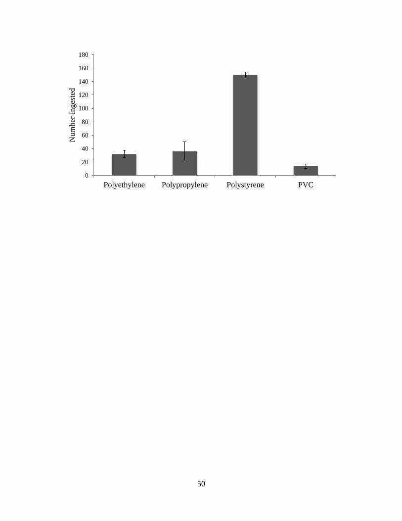
Plastic particulates were ingested by A. troschelii. Polystyrene was ingested at a

significantly higher level than the other plastics (Table 1, ANOVA, F3, 48 = 27.8985, p =

< 0.001). The total number of polystyrene particles ingested was four times greater than

the total number of polypropylene particles ingested, five times greater than the total

number of polyethylene particles ingested, and eleven times greater than the total number

of polyvinyl chloride particles ingested (Figure 1). The plastic that had the least overall

amount ingested was polyvinyl chloride and had an average ingestion rate of 4.67

particulates/trial (Figure 1). Polypropylene particles had an average ingestion rate of 12

particulates/trial, polyethylene had an average ingestion rate of 10.67 particulates/trial,

and polystyrene had an average ingestion rate of 50 particles/trial (Figure 1).

Juvenile A. troschelii ingested more plastic particulates than adults (Table 1,

ANOVA, F1, 48 = 22.2000, p = <0.001). The difference lies within the fact that juveniles

ingested significantly more polystyrene than the adults (Table 1, F3, 48 = 24.1315, p =

<0.001). While the three other plastics (polyethylene, polypropylene, and polyvinyl

chloride) showed no major differences in overall plastic ingested between the two life

stages, juveniles ingested 7.33 times more polystyrene than the adults (Figure 2).

There was a significant difference in plastic ingested due to color (Table 2, ANOVA,

F10, 143 = 5.3331, p = < 0.001). The plastics that were ingested the most were pink

polyethylene pieces, followed by white polypropylene pieces and red polypropylene

pieces (Figure 3). There were no black polyethylene pieces ingested and no blue pieces

were ingested of either plastic (Figure 3). There was a significant relationship between

37

color of plastic and type of plastic ingested (ANOVA, F1, 143 = 5.5000, p = 0.0204). This

was because there was a lot more white polypropylene particles ingested than white

polyethylene pieces ingested (Figure 3). The average amount of white polypropylene

ingested was thirteen times greater than the average amount of white polyethylene

ingested (Figure 3).

This experiment lasted three days, or three trials, and we found no significant

relationship between plastics ingested and trial number (Table 3, ANOVA, F2, 64 = 0.789,

p= 0.4623). However, the overall amount of plastics ingested increased with each trial

(Figure 4).

Discussion

Our first hypothesis that A. troschelii would ingest planktonic-sized

thermoplastics was supported. Due to their planktivorous diet (Kerr, et al. 2014), they

were more likely to confuse the plastics we tested on them for prey. Planktivorous

organisms have a higher incidence of ingesting plastics than piscivores (Derraik, 2002).

In other studies conducted in the North Pacific Central Gyre, large concentrations of

micro-plastics are mixing with planktivorous organisms’ food sources (Boeger, et al.,

2010). About 35% of the mesopelagic planktivorous fishes surveyed after six night trawls

had plastic pieces in their guts (Boeger, et al., 2010). Due to the buoyancy of micro-

plastics, they are easily suspended within the water column and intermixed with surface

food sources making it difficult for fish to distinguish between the plastic and their prey

(Morris, 1980; Boeger, et al., 2010; Derraik, 2002).

38

We found a difference between the amount of plastic ingested by the juveniles

and adults, thus supporting our second hypothesis. However, the reason was not proved

to be because of their differing metabolic rates. Our results can be attributed to the

physical and dietary changes of A. troschelii throughout their lifetime (Frederich, 2007).

Most reef fish undergo what is called an ontogenetic modification in their diet (Frederich,

2008). This modification is stimulated by their interactions with fluctuating external

factors such as habitat, food supply, and predation risk (Grutter, 2000). This in turn

affects their internal conditions such as anatomical structures, behavior and physiological

demands (Frederich, 2008). During the lifetime of A. troschelii, ontogenetic

modifications alter their physiological structures, such as the size and the shape of their

mouth (Frederich, 2007). Juveniles swim closer to the surface feeding on minute

organisms; therefore their mouths are small and simple in structure (Hobson, 1965). As

they mature, they begin to forage over the rocky bottom causing the size of their mouth to

grow and the shape of their mouth to change (Frederich, 2007).

The juveniles ingested more polystyrene particles than the adults. Panamic

sergeant major juveniles are known to deliberately aggregate around and feed on floating

objects (Nelson, 2003). The highly buoyant nature of polystyrene and its ability to

fragmentize into small pieces creates an ideal situation for ingestion by juvenile A.

troschelli (Davidson, 2012). This plastic has a high affinity for PAHs (Polycyclic

aromatic hydrocarbons) and, if consumed, these toxins are capable of transferring

carcinogenic and endocrine disrupting monomers to the organism (Rochman et al.,

2013b). Polystyrene is often found floating under docks and is known to expel millions of

micro-plastic particulates due to the boring of isopods (Davidson, 2012).

39

There was a preference in the color of plastic ingested, thus supporting our third

and final hypothesis. However, the colors we thought A. troschelii more likely to ingest

were clear, white, or green and that was inaccurate. The most preferred colors of plastic

by both juveniles and adults were pink, followed by white, and red. In the bay of

Pichilingue, one of the main food sources of A. troschelii is fish eggs, which are known

to have different color tones ranging between clear, white and pink (Garcia-Lopez, et al.

2004; Zavala-Leal, 2007). Small planktonic crustaceans from this area of the bay are

green and red-orange in color (Aceves-Medina, 2007). This could have been the reason

that A. troschelii ingested more red and polypropylene. Following the ingestion of pink,

red and white, the green colored polyethylene was of interest to the fish. Since

polyethylene is a low-density plastic and floats on the surface, this could have resembled

the green microalgae found in A. troschelii’s diet (Moreno-Sanchez, 2009).

We found that white polypropylene was preferred over white polyethylene. This

could have been due to the densities of the plastics, however we found no research on

preferences for plastic densities. Another reason could be that with the polyethylene, the

fish were given seven other colors to choose from, while with the white polypropylene

there were only three other colors, thus increasing the likelihood that they would eat the

white polypropylene.

This experiment only lasted three days so we were unable to find any long-term

effects of plastic ingestion in the fish. However, hydrophobic organic contaminants have

a greater affinity for polyethylene, polypropylene and PVC compared to natural

sediments (Teuten et al., 2009). These plastics carry POPs (Persistent Organic Pollutants)

and other studies have shown that these toxins can bioaccumulate in an animal if plastics

40

containing them are ingested and can directly affect the health of that animal (Rios, et al.

2007). Polypropylene in the marine environment can adsorb and transport PCBs, DDE

and nonylphenols (Moore, 2008) while polystyrene has been known as a source and sink

for PAH’s (Polycyclic aromatic hydrocarbons) in the marine environment (Rochman et

al., 2013b). There is also the threat of indirect consumption of these chemicals by higher

trophic level organisms via predation on animals that initially ingested the plastic. The

yellow snapper is a predator of the species Abudefduf troschelii (Vazques, et al. 2008),

and is also a species commonly served in many restaurants in the La Paz area. If the

yellow snapper were to eat a toxic fish, then there is a chance that humans would

eventually consume the same toxins initially transferred by the consumption of plastics in

our ocean. More research conducted on topics relating to plastic ingestion will provide

input for conservation management, support the foundation for educational campaigns,

and also provide other scientists with better evidence to demand more effort to mitigate

the problem from the authorities (Derraik, 2002).

For future experiments, it would increase the well being of the test subjects if a

softer type of netting was used. A reason there may have been error in our experiment

was due to the collection method. For future experimentation it would be beneficial to

have more people observing the cage at the same time and a more efficient form of

plastic delivery.

41

Acknowledgements

We would like to formally thank Ben Miner, Alejandro Acevedo, Sergio Flores and Deb

Donovan for supporting us and helping us develop this project. We would also like to

thank our colleague, Erin Matthews, for helping us capture the fish used for this project.

References

Aburto-Oropeza, O., Sala E. and Sánchez-Ortiz C., 2000. Feeding behavior, habitat use,

and abundance of the angelfish Holacanthus passer (Pomacanthidae) in the

southern Sea of Cortés. Environmental Biology of Fishes 57:435-442.

Aceves-Medina G., Esqueda-Escárcega G. M., Pacheco-Chávez R., Zárate-Villafranco

A., Hernández-Alonso J. R and Hernández-Trujillo S. 2007. Cambios diarios en la

composición y abundancia de copépodos planctónicos al sur de Bahía de La Paz.

Hidrobiológica 17(2): 185-188

Boerger C. M., Lattin G. L., Moore S. L. and Moore C. J. 2010. Plastic ingestion by

planktivorous fishes in the North Pacific Central Gyre. Marine Pollution Bulletin

60: 2275–2278

Cózar, A., Echevarría, F., González-Gordillo, I.J., Irigoien, X., Úbeda, B., Fernández-de-

Puelles, Álvaro, P.T., Navarro, S., García-de-Lomas, J., Ruiz, A., Fernández-de-

Puelles, M.L., Duarte, C.M. Plastic debris in the open ocean. Proceedings of the

National Academy of Sciences 111(28): 10239-10244.

42

Davidson T. M. 2012. Boring crustaceans damage polystyrene floats under docks

polluting marine waters with microplastic. Marine Pollution Bulletin 64: 1821–

1828

Derraik J. G. 2002. The pollution of the marine environment by plastic debris: a review.

Marine Pollution Bulletin 44: 842–852

Foster S.A. 1987. Diel and lunar patterns of reproduction in the Caribbean and Pacific

sergeant major damselfishes A budefduf saxatilis and A. troschelii. Marine

Biology 95: 333-343

Frederich, B. Adriaens, D., Vandewalle, P. 2008. Ontogenetic shape changes in

Pomacentridae (Teleostei, Perciformes) and their relationships with feeding

strategies: a geometric morphometric approach. Biological Journal of the Linnean

Society 95: 92-105.

Garcia-Lopez V., Rodriguez-Romero A., and Perez-Ramirez J. M. 2004. Induccion al

desove con HGC y desarrollo embrionario de larvas de la cabrilla sardinera

Mycteroperca rosacea (Streets, 1877). Ciencias Marinas. 30 (2): 279-284

Grutter A. S. 2000. Ontogenetic variation in the diet of the cleaner fish Labroides

dimidiatus and its ecological consequences. Marine Ecology Progress Series. 197:

241-246

Hammer J., Kraak M. H. And Parsons J. R. 2012. Plastics in the maine environment. The

dark side of modern gift. In: Reviwes of envirinmenal contamination and

toxicology. Springer Science. USA. 44 pp.

43

Hobson E. S. 1965. Diurnal-Nocturnal Activity of Some Inshore Fishes in the Gulf of

California. COPEIA 3: 291-302

Ivar do Sul J. A. and Costa M.F. 2014. The present and future of microplastic pollution in

the marine environment. Environmental Pollution 185: 352-364

Kerr K. A., Cornejo A., Guichard F. and Collin R. 2014. Planktonic predation risk varies

with prey life history stage and diurnal phase. Marine Ecology Progress Series

503: 99–109.

Moore C. J. 2008. Synthetic polymers in the marine environment: A rapidly increasing,

long-term threat. Environmental Research 108: 131–139

Moreno-Sanchez X. G. 2009. Estructura Y Organización Trófica De La Ictiofauna Del

Arrecife De Los Frailes, B.C.S. México. Doctoral Thesis. Cicimar-IPN. México.

143 pp.

Morris, R.J. 1980. Plastic Debris in the Surface Waters of the South Atlantic. Marine

Pollution Bulletin 11:164-166.

Nelson P. A. 2003. Marine fish assemblages associated with fish aggregating devices

(FADs): effects of fish removal, FAD size, fouling communities, and prior

recruits. Fishery Bulletin. 101:835–850.

Rios L. M., Moore C. and Jones P. R. 2007. Persistent organic pollutants carried by

synthetic polymers in the ocean environment. Marine Pollution Bulletin 54:

1230–1237

44

Rochman C. M., Hoh E., Kurobe T. and Teh S. 2013a. Ingested plastic transfers

hazardous chemicals to fish and induces hepatic stress. Scientific Reports 3: 3263

Rochman C. M., Manzano, C., Hentschel, B. T., Massey S. L. and Hoh E. 2013b.

Polystyrene Plastic: A Source and Sink for Polycyclic Aromatic Hydrocarbons in

the Marine Environment. Environmental Science & Technology 47:

13976−13984.

Teuten E. L., Saquing J. M., Knappe D., Barlaz M.A, Jonsson S., BjÖrn A., Rowland S.

J., Thompson R. C., Galloway T. S., Yamashita R., Ochi D., Watanuki Y., Moore

C., Viet P. H., Tana T. S., Prudente M., Boonyatumanond B., Zakaria M. P.,

Akkhavong K., Ogata Y., Hirai H., Iwasa S., Mizukawa K., Hagino Y.,

Imamura1A., Saha M. and Takada H. 2009. Transport and release of chemicals

from plastics to the environment and to wildlife. Philosophical Transactions of the

Royal Society B 364: 2027–2045.

Vázquez R. I., Rodríguez J., Abitia L. A. and Galván F. 2008. Hábitos alimenticios del

pargo amarillo Lutjanus argentiventris (Peters, 1869) (Percoidei: Lutjanidae) en la

Bahía de La Paz, México. Revista de Biología Marina y Oceanografía 43(2): 295-

302.

Zavala-Leal O. I. 2007. Efecto de la temperatura, intensidad de luz, tipo y densidad de

presa en la eficiencia alimenticia durante la ontogenia inicial del huachinango del

pacifico (Lutjanus peru). Master degree thesis. CICIMAR, La Paz B.C.S. México.

52 pp.

45

Table 1. A blocked 2 factor ANOVA was performed and tested the variance within life

stage of A. troschelii (“Stage”), cage number (“Cage”), and type of plastic ingested

(“Plastic”). It also tested the relationships between life stage and plastic type ingested

(“Stage : Plastic”) and cage number and type of plastic ingested (“Cage : Plastic”).

Degrees of

Freedom

Sum

Squared

Mean

Squared

F-Value

P-Value

Stage

1

171.13

171.125

22.2000

<0.001

Cage 4 33.50 8.375 1.0865 0.3738

Plastic 3 645.15 215.051 27.8985 <0.001

Stage : Plastic 3 558.04 186.014 24.1315 <0.001

Cage : Plastic 12 64.06 5.338 0.6925 0.7503

Residuals 48 370.00 7.708

46

Table 2. A blocked 2 factor ANOVA was performed and tested the variance within life stage of A. troschelii (“Stage”), type of plastic ingested (“Plastic”), cage number (“Cage”), and color of plastic ingested (“Color”). It also tested the relationships between life stage and plastic type ingested (“Stage : Plastic”), cage number and type of plastic ingested (“Plastic : Cage”), life stage and color of plastic ingested (“Stage : Color”), type of plastic ingested and color of plastic ingested (“Plastic : Color”), and cage number and color of plastic ingested (“Cage : Color”). The relationship between life stage, plastic type, and plastic color (“Stage : Plastic : Color”) as well as the relationship between plastic type, cage number, and plastic color (“Plastic : Cage : Color”) were also tested.

Degrees of

Freedom

Sum

Squared

Mean

Squared

F-Value

P-Value

Stage

1

0.024

0.02436

0.0670

0.79616

Plastic 1 1.780 1.78041 4.8961 0.02850

Cage 4 0.205 0.05133 0.1412 0.96661

Color 9 14.837 1.64858 4.5336 <0.001

Stage : Plastic 1 0.160 0.15954 0.4387 0.50880

Plastic : Cage 4 0.374 0.09356 0.2573 0.90482

Stage : Color 9 4.211 0.46793 1.2868 0.24895

Plastic : Color 1 2.000 2.00000 5.5000 0.02039

Cage : Color 36 5.862 0.16283 0.4478 0.99693

Stage : Plastic : Color 1 0.222 0.22222 0.6111 0.43566

Plastic : Cage : Color 4 0.444 0.11111 0.3056 0.87388

Residuals 143 52.000 0.36364

47

Table 3. A blocked 1 factor ANOVA was performed and tested variance within cage

number (“Cage”) and trial number (“Trial”).

Degrees of

Freedom

Sum

Squared

Mean

Squared

F-Value

P-Value

Cage

5

204.62

40.925

1.6388

0.1625

Trial 2 39.00 19.500 0.7809 0.4623

Residuals 64 1598.25 24.973

48

Figure Captions

Figure 1. Total ingestion of plastic particulates by A. troschelii over a timespan of three

days with one trial/day. Plastic particulates were 1mm-5mm in diameter. The four types

of plastic that were ingested were two low density plastics: polyethylene and polystyrene

and two high density plastics: polypropylene and polyvinyl chloride (PVC). Error bars

show standard deviation (n=6).

Figure 2. Total number of plastic particulates ingested by juveniles and adults from all

three trials. Plastics ingested were polyethylene, polypropylene, polystyrene, and

polyvinyl chloride. Error bars show standard error (n=6).

Figure 3. Average number of colored plastic particulates ingested by both juveniles and

adults from all three trials. The thermoplastics ingested were polyethylene: a low density

thermoplastic and polypropylene: a high density thermoplastic. There were eight tested

colors of polyethylene and four tested colors of polypropylene.

Error bars show standard error (n=6).

Figure 4. Total number of plastic particulates ingested by A. troschelii during three trials

where there was one trial/day. This data incorporates all four plastics: polyethylene,

polystyrene, polypropylene, and polyvinyl chloride. Error bars show standard deviation

(n=6).

49

0

20

40

60

80

100

120

140

160

180

Polyethylene Polypropylene Polystyrene PVC

Num

ber I

nges

ted

50

51

52

0

20

40

60

80

100

120

140

Trial 1 Trial 2 Trial 3

Num

berIn

gest

ed

53

Haplotype frequencies of Green Sea Turtles (Chelonia mydas)

involved in a mass die-off event along the western coast of

Baja California Sur, Mexico.

MacKenzie Gwinn, Emily Hiatt, Mallory Ogburn

Western Washington University

Abstract

Green sea turtles (Chelonia mydas) are found all over the world, and are an

endangered species that has experienced severe population decline. Causes of this

decline are often anthropogenic. The green sea turtle populations of Baja California have

been subjected to poaching, bycatch, and pollution and their numbers have dropped to

mere fractions of what they once were. In this study, we look at a mass mortality event

that occurred in Laguna Ojo de Liebre in February 2011. Our question focused on the

population structure of the turtles that died in this event, which we analyzed using

mitochondrial DNA from tissue samples. We predicted that our sample haplotypes would

be found in a variety of different rookeries in the Pacific Ocean. DNA from the tissue

was extracted, amplified, and sequenced from 11 individuals found washed up on the

beach. The mitochondrial DNA sequences were analyzed and run through BLAST to

determine which haplotype and rookery they belonged to. Seven of the individuals had

the haplotype CMP5 and every haplotype we had has been found at the Michoacán

rookery on the Pacific coast of Baja California. That the Michoacán rookery is

54

geographically close to the foraging grounds of Ojo de Liebre could be a possible

explanation for this result. Other explanations include a virus or environmental factor at

the nesting grounds that selectively affected the haplotypes found at Michoacán.

Whatever the cause, a considerable number of East Pacific Green Turtles died at Ojo de

Liebre. Conservation efforts need to not only focus on nesting grounds but also on the

foraging grounds of this species.

55

Introduction

Green Sea Turtles (Chelonia mydas) are found worldwide between 30°N and

30°S in tropical and subtropical waters (Bowen et al., 1992). The large-scale population

structure of green turtles depends on the natal homing behaviors of females, as they

return to their original nesting grounds to lay eggs (Hirth, 1997). This behavior creates a

distinct matrilineal structure at each rookery (Formia et al., 2007), and has affected the

evolution of worldwide green turtle phylogenic subsets, including the East Pacific

(known as the “black turtle”,) and the Atlantic-Mediterranean form (Bowen et al., 1992).

In this study, we focus on East Pacific Green Turtles (EPGT), which nest in the main

rookeries of the French Frigate Shoals, Galapagos Islands, Revillagigedos Archipelago

and Michoacán, Mexico (Chassin-Noria et al., 2004).

The World Conservation Union (IUCN) currently lists green sea turtles as

endangered throughout their range. Presently, illegal fishing, habitat loss and pollution

threaten the global populations of green turtles (Kasparek et al., 2001; Cliffton et

al.,1982). Data on the population numbers of rookeries, and rookery trends, such as

migration patterns of EPGT, are crucial to properly manage their recovery (Wallace et al,

2010). Throughout the life cycle of EPGT, migration occurs from the nesting grounds to

pelagic or neritic foraging habitats (Reich et al., 2007). This movement leads to feeding

grounds having a heterogeneous array of green turtle individuals from many different

populations (Luke et al., 2004). Therefore, the loss of foraging habitat and mortality of

turtles in these areas can negatively affect many different populations of EPGT

(Amorocho et al., 2012).

56

Genetic sampling of haplotype frequencies in foraging grounds has proved

successful in quantifying how many turtles in a feeding area are from a specific rookery

and how they are being affected by human impacts (Dutton et al. 2008). This technique

has proved successful in identifying genetic differences between the foraging and nesting

aggregations of turtles in many areas. Dutton et. al (2008) used haplotype analysis to

determine the nesting origin of green turtles in foraging grounds in Hawaii. The results of

this analysis led them to conclude that the foraging populations were from one genetic

stock from French Frigate Shoals nesting grounds, which had implications for

management of Hawaiian green turtles. In this study as well as others, mitochondrial

DNA (mtDNA) was used instead of nuclear DNA to determine population structure.

Mitochondrial DNA is more useful because the populations follow a matrilineal structure

and mtDNA is passed to the offspring from the mother (Amorocho et al., 2012).

Therefore, the haplotypes of the mtDNA can supply insight into which specific rookeries

the turtles hatched at (Dutton et al., 2008).

This technique has also been useful in analyzing the sea turtle population structure

in the foraging grounds off the western coast of Baja California Sur, Mexico (Nichols,

2003). The coastal lagoons in this region serve as sheltered feeding grounds for juvenile

sea turtles, while exposed coastal areas have higher proportions of adult EPGTs (Lopez-

Mendilaharsu et al. 2005). Many conservation groups have identified these areas as

critical feeding grounds for EPGT because of the mixed age groups and habitats in this

region. However, there has been no specific action taken by the government of Mexico

towards protecting these areas and the EPGT populations continue to decline (Lopez-

Mendilaharsu et al. 2005). The main causes of mortality in this region have been

57

attributed to fishing, either poaching or bycatch from gill nets in the region (Koch et al.,

2006). It has been estimated that over 3,000 EPGTs are slaughtered each year for the

purpose of human consumption and a minimum of about 1,500 are annually killed from

bycatch (Koch et al., 2006; Mancini et al., 2012).

In this study, we attempt to distinguish the population identity of green turtles that

were found washed up on a beach on the western coast of Baja California Sur. The turtles

were found all at once and numbered over 200 individuals, which implied that this was a

mass mortality event. The event occurred in February of 2011 in the lagoon foraging

grounds of Ojo de Liebre. When researchers examined the turtles they displayed

significant signs of decomposition, so the exact day or temporal spread of mortality in

this event is unknown. Approximately 30 tissue samples were taken from different sea

turtles that were washed up on the beach.

In order to determine which populations these turtles belonged to, we performed

haplotype analysis on tissue samples collected from 15 of the deceased turtles. We

analyzed the mtDNA of the turtles to determine which rookery they belonged to. We

hypothesized that the turtles sampled from this event are from different nesting

populations, based on the assumption that the feeding grounds around Ojo de Liebre

would display the same heterogeneity of EPGT that is found in other foraging areas. The

results of this study increase our understanding of population recovery rates of rookeries

in the area, and inform conservationists and managers about the populations that were

negatively affected by this event.

58

Methods

For this study, we extracted DNA, performed PCR on, and received sequences on

17 green sea turtle tissue samples from a mass die off at Ojo de Liebre Lagoon that

occurred in February 2011. Two samples were from a stranding that was not during the

mass die off, and was tested for a comparison. Each of the 17 original samples was

macerated and placed in an 1 ml epitube containing 300 μl of an extraction buffer, which

contained 100 mM NaCl, 50 mM Tris-HCl, 15 SDS, and 50 mM EDTA. We added 10 μl

of proteinase-K to each sample while stirring and incubated them at 65°C for

approximately two hours. Some of the samples were not fully degraded after the

incubation period, so they were mashed manually and 5 more microliters of proteinase-K

were added. Once the samples were fully degraded, 300 μl of LiCl was added to each of

the tubes and were continuously inverted for one minute. Samples 4, 5, 10, 8, and 9 had

the chloroform added before the LiCl. We performed three consecutive washes, the first

and last using Chloroform: Isoamyl Alcohol (24:1), the second using Phenol:

Chloroform: Isoamyl Alcohol (25:24:1). For each wash, the chloroform mixture was

added and the tubes were vortexed for 10 seconds. Each tube was then rotated for 30

minutes and placed in a centrifuge for 15 minutes. Once out of the centrifuge, the upper

aqueous layer was carefully removed from the lower chloroform layer and placed in a

new tube and the process was repeated.

After the third wash, 1000 μl of cold 95% ethanol and 50 μl of Sodium Acetate

3M was added to each tube and inverted several times. The tubes then sat for 12 hours at

-20°C, allowing the DNA to precipitate. Each tube was then centrifuged and the ethanol

was poured off, leaving the DNA pellet. Seven hundred fifty μl of cold 70% ethanol was

59

added to each tube and centrifuged again. Excess ethanol was discarded and the DNA

pellet was dried at 55°C. The remaining DNA pellets were then re-suspended in 50 μl of

TE buffer solution. Gel electrophoresis was then performed in an ETBr 1% agarose gel

to verify the quality of the DNA by evaluating the brightness of the DNA lines. Tubes

T10, T12, T19, T24, T26, and T20 still contained chloroform from the washing steps,

which made performing PCR on them unviable as the chloroform encases the DNA, not

allowing the necessary reactions to take place. PCR was not done on these samples, and

they were excluded from the rest of the analysis.

A PCR cocktail was prepared using 402.5 μl water, 57.5 μl buffer, 11.5 μl dNTPs,

23 μl MgSO4, 23 μl Primer R, 23 μl Primer F, and 4.6 μl Taq polymerase. The primers

used were HDCM2 and LTCM2, which are designed to target the 488 bp at the 5’ end of

the mitochondrial genome control region (Dutton et al 2008). Twenty-four microliters of

this cocktail was added to 1 μl of DNA from each original samples. There were two PCR

tubes for each sample. The tubes were put through a thermocycler program for 35 cycles

that lasted a total of 2 hours 5 minutes. Another Gel Electrophoresis was done on the

PCR products to verify DNA quality. Those samples with high quality DNA were then

sent to a lab for nucleotide sequencing.

After receiving the nucleotide sequences, we used Clustalx to test the quality of

the DNA and to verify that the forward and reverse sequences were from the same

sample. The forward and reverse sequences of dirty or overly decayed DNA would not

be complimentary. All eleven of the samples had complimentary forward and reverse

sequences. Each sequence was then put through the program BLAST which matched our

sequences to existing ones to determine the haplotype of the turtle. We used data from

60

Dutton et al. (2008) to determine the rookery locations at which each haplotype is

typically found.

Results

Five different haplotypes were identified from the 11 individuals sampled (Table

1). All of the haplotypes found occur in rookeries in the east Pacific. Seven of the ten

turtles samples from the Ojo de Liebre die off had the CMP5 haplotype. Dutton et al.

(2008) only found this haplotype in individuals at the Michoacán rookery. The other two

haplotypes found were CMP7 and CMP12, which are both from the Michoacán rookery.

All other haplotypes in our samples from the die off occur in the Michoacán rookery.

The sample labeled T3 had the haplotype CMP4 (Table 1). This haplotype is on of the

most common in Michoacán rookery, but has also been found in individuals from the

rookeries of the Galápagos Islands and Revillagigedos Archipelago (Dutton et al., 2008).

Sample 4 was not from the die off event, but stranded further south on the Baja

Peninsula. The haplotype from sample 4 was CMP8, which also occurs in the Michoacán

rookery, which suggests that many individuals along the entire Baja Peninsula coast are

from this rookery.

Discussion

Our hypothesis was not supported by the results of this analysis, as the green

turtles sampled all had haplotypes that are found in a single rookery. The only evidence

of an individual belonging to another rookery population was found in sample T3, where

there was uncertainty in the nesting population it belonged to, although it is very likely

that it is from the Michoacán rookery. In the remaining samples, there was variance

61

within the haplotypes of the individuals even though the haplotypes all corresponded to

the Michoacán rookery. In a study by Chassin-Noria et al. (2004), they found that

Michoacán has two common haplotypes (CMP4 and CMP5) and three uncommon

haplotypes (CMP7, CMP8 and CMP12). However, the population of all the beaches

within Michoacán did not show significant genetic sub-structuring when the mtDNA of

nesting females was tested. Therefore, it is not unreasonable to conclude that all of the

individuals we sampled that had haplotypes from Michoacán belonged to a single

population.

Since Michoacán is one of the closest rookeries to Ojo de Liebre, these results

may be explained simply by the proximity between the nesting and foraging grounds.

Also, Michoacán is the second largest rookery in this area, only surpassed recently by the

Galapagos rookeries (Chassin-Noria, 2004). This could justify our results that all the

sampled turtles belong to this population. There are no previous studies on haplotype

frequency and population structure of green turtles in this region. Therefore, we can’t

compare our results to a larger sample size and determine if our results mirror the

population structure of the foraging turtles that were not impacted by this event.

The source of deviation between our results and predictions in this study may

have been due to our assumptions when forming our hypothesis. We determined it likely

that the Baja foraging ground population structure would show the same heterogeneity as

other regions often show based on previous research. However, in a previous study on

population structure in Hawaiian green turtle populations, Dutton, et al. (2008) found

there to be less mixing of haplotypes than most studies in other foraging areas. The

results of this study indicated that in this foraging ground, there was a large majority of

62

turtles that belonged to one population, and a significantly lower amount turtles that

belonged to different populations (Dutton et al. 2008). With our small sample size, we

may have experienced a skew in the turtles sampled that only reflected the major

population component of the 200 turtles that were impacted by this event. Also, from our

results, we can’t exclude the possibility that this event was specific to the haplotypes

affected. Mortality causes, such as viruses or factors from the nesting grounds, may have

been responsible for the selective death of these green sea turtles from the Michoacán

rookery.

Though we can’t extrapolate the data from these individuals to the entire mass

die-off event, the results clearly indicate that the population of Michoacán was decreased

by some unknown degree during this occurrence. These results have implications for the

conservation of nesting EPGT in Michoacán, as it indicates mortality of individuals in

their foraging grounds. This rookery was heavily overfished in the 1960’s and 1970’s for

consumption of green turtles in the Northern areas of Mexico (Chassin-Noria et al.,

2004). This exploitation resulted in the population of nesting females in this area to drop

from 25,000 to 1,400 in the 1980’s (Chassin-Noria et al. 2004). In 1986, the beaches in

Michoacán were declared a natural reserve area in order to protect the EPGT nesting

grounds (Alvarado-Diaz et al. 2001). However, this population continued to decline

through 1999, and because of the slow-growth rate of individuals, is still considered

endangered and vulnerable to extinction (Seminoff et al., 2002). Without proper

management of foraging grounds for this population, it is unlikely that the population will

recover to its original numbers. Human threats such as bycatch, poaching and habitat

destruction of foraging grounds can have great impacts on the recovery rate of this

63

population, and in order to encourage population recovery, both lawmakers and

communities should enforce protection of these areas.

Future studies on large mortality events should be continued in order to analyze

the population structure of turtles killed, providing information on the affected

populations and therefore rookeries. Emphasis should be placed on collecting adequate

sample sizes that can provide broader picture of precisely which populations are being

affected by these events. Haplotype sampling in this foraging region would be greatly

beneficial to future research in determining a baseline population structure of turtles.

Also, research on the causes of mass mortality events should be conducted to determine

what steps can be taken to avoid losses of green turtles in the future.

The preservation of green turtle populations worldwide has been a cause of

concern for researchers and conservationists. In order to fully manage and continue the

protection of this species, efforts have to focus not only on the nesting behavior and

breeding areas of green turtles, but also the foraging grounds. The preservation of

foraging populations is based in enforcing poaching and bycatch laws, reducing habitat

loss and carefully tracing the dynamics and numbers of each population of EPGT. A

collaboration of data on the threats to the EPGT in both nesting and foraging habitats is

necessary to preserve this charismatic megafauna.

64

References

Alvarado-Diaz, J., C. Delgado-Trejo and I. Suazo-Ortuno. 2001. Evaluation of the Black

Turtle Project in Micoacan, Mexico. Marine Turtle Newsletter. 92: 4-7.

Amorocho, D. F., F. A. Abreu-Grobois, P. H. Dutton, R. D. Reina. 2012. Multiple distant

origins for green sea turtles aggregating off Gorgona Island in the Colombian

Eastern Pacific. PLoS ONE. 7(2).

Bowen, B.W., A.B. Meylan, J.P. Ross, C.J. Limpus, G.H. Balazs and J.C. Avise. 1992.

Global population structure and natural history of the green turtle (Chelonia

mydas) in terms of matriarchal phylogeny. Evolution. 46(4):865-881.

Chassin-Noria, Omar, Alberto Abreu-Grobois, Peter H. Dutton, and Ken Oyama. 2004.

Conservation genetics of the east Pacific green turtle (Chelonia mydas) in

Michoacan, Mexico. Genetics 121:195-206

Dutton, Peter H., George H. Balazs, Robin A. LeRoux, Shawn K. K. Murakawa, Patricia

Zarate, and Laura Sarto Martínez. 2008. Composition of Hawaiian green turtle

foraging aggregations: mtDNA evidence for a distinct regional population.

Endangered Species Research 5:37-44.

Formia, Angela, Annette C. Broderick, Fiona Glen, Brendan J. Godly, Graeme C. Hays,

and Michael W. Bruford. 2007. Genetic composition of the Ascension Island

green turtle rookery based on mitochondrial DNA: implications for sampling and

diversity. Endangered Species Research 3:145-158.

Hirth, F.H., 1997. Synopsis of the Biological Data on The Green Turtle, Chelonia mydas

65

(Linnaeus, 1758). Biological Report, 97(1).

Kasparek, M., B.J. Godley, A.C. Broderik. 2001. Nesting of the Green Turtle, Chelonia

mydas, in the Mediterranean: a review of status and conservation needs. Zoology

in the Middle East. 24(1):45-74.

Koch, V., Nichols, W.J., Peckham, H., and de la Toba, V. 2006. Estimates of sea turtle

mortality from poaching and bycatch in BahÍa Magdalena, Baja California Sur,

Mexico. Biological Conservation. 128(3):327-334.

Lopez-Mendilaharsu, M., S.C. Gardner, A.S. Jeffry and R. Riosmena-Todriguez. 2005.

Identifying critical foraging habitats of the green turtle (Chelonia mydas) along

the Pacific coast of the Baja California peninsula, Mexico. Aquatic Conservation:

Marine and Freshwater Ecosystems. 15:259-269.

Luke, K., J.A. Horrocks, R.A. LeRoux, P.H. Dutoon. 2004. Origins of green turtle

(Chlonia mydas) feeding aggregations around Barbados, Wester Indies. Marine

Biology. 144(4):799-805.

Mancini, A., V. Koch, J.A. Seminoff and B. Madon. 2012. Small-scale gill-net fisheries

cause massive green turtle Chelonia mydas mortality in Baja California Sur,

Mexico. Oryx. 46(1):69-77

Nichols, W.J. 2003. Biology and conservation of sea turtles in Baja California, Mexico.

The University of Arizona.

Reich, K.J., K.A. Bjorndal and A.B. Bolten. 2007. The ‘lost years’ of green turtles: using

stable isotopes to study cryptic lifestages. Biology Letters. 3:712-714.

66

Seminoff, J.A., A. Resendiz, W.J. Nichols and T.T. Jones and C. Guyer. 2002. Growth

rates of wild green turles (Chelonia mydas) at a temperate foraging area in the

Gulf of California, Mexico. Copeia. 2002(3):610-617.

Wallace, B.P., A.D. DiMatteo, B.J. Hurley, E.M. Finkbeiner, A.B. Bolten, M.Y.

Chaloupka, B.J. Hutchinson, F. A. Abreu-Grobois, D. Amorocho, K. A. Bjorndal,

J. Bourjea, B.W. Bowen, R. Briseño Dueñas, P. Casale, B.C. Choudhury, A.

Costa, P.H. Dutton, A. Fallabrino, A. Girard, M. Girondot, M.H. Godfrey, M.

Hamann, M. López-Mendilaharsu, M.A. Marcovaldi, J.A. Mortimer, J.A. Musick,

R. Nel, N.J. Pilcher, J.A. Seminoff, S. Troëng, B. Witherington, R.B. Mast. 2010.

Regional Management Units for Marine Turtles: A Novel Framework for

Prioritizing Conservation and Research across Multiple Scales. PLoS ONE 5(12)

67

Table 1 Green sea turtle haplotypes and nesting populations of the 10 individuals

sampled from a mass die off event in Ojo de Liebre lagoon, February 6, 2011. Individual

with haplotype CMP8 was not from the event, and was found stranded along the west

coast of Baja California on a different date.

68

Figure 1 A map of Ojo de Liebre, the location of the mass die-off event of green turtle’s

in Baja California Sur, Mexico.

69

Alarm response in Centrostephanus coronatus with increasing exposure to the predatory chemosensory cues of Heliaster kubiniji

Brittany Weiss, Denielle Beenken, Jessica Stanley

Western Washington University

516 High Street Bellingham, WA 98225

70

Abstract

In marine environments, predators and prey emit and respond to chemosensory cues.

In many cases, prey species have evolved the ability to detect these cues which can help them

avoid predation by fleeing or use of other behavioral responses. This study focused on the

possible acclimation of the Crowned sea urchin, Centrostephanus coronatus to cues emitted

by the predatory Gulf sun star, Heliaster kubiniji. Behavioral alarm responses of C.

coronatus, were measured in the field when contact was made with H. kubiniji, and

compared to alarm responses exhibited when contact was made with the non-predatory Tan

sea star, Phataria unifascialis. Responses to the predatory species were significantly greater

than responses to the non-predatory species, supporting that C. coronatus detects

chemosensory cues produced by its predator, H. kubiniji. To determine if the C. coronatus

acclimated to its predator’s presence, urchins were placed in tanks with H. kubiniji and

separated by a mesh barrier. The behavioral responses of the urchins to contact with the sun

star were measured at varying times of exposure, up to 40 minutes. No significant

relationship was found between the response of C. coronatus and the time of exposure to its

predator. This shows that in 40 minutes, C. coronatus does not acclimate to the predatory

chemosensory cues of H. kubiniji. These species are known to live in close proximity with

one another. In order to utilize energy efficiently, C. coronatus has evolved to expend energy

only in the presence of species that are a direct threat and to sense cues for an extended

period of time. These both are favorable for the fitness of C. coronatus.

71

Introduction

In any given niche, a complex hierarchical web exists, shaped by the coevolution of

predators and prey. Traits involved in predation are subject to strong selection forces because

survival is critically dependent on avoidance of predators as well as success in finding food

(Abrams 2000). The coevolution of predator and prey occurs in a cyclical fashion where

species must adapt to maximize fitness for a given environment so they can successfully

forage, reproduce, and escape predation (Abrams 2000). These changes are slow to develop,

as they occur through natural selection over evolutionary time periods. However, some

species may be able to acclimatize behaviorally within their own lifetimes. Like adaptations

over an evolutionary time scale, behavioral changes within an individual’s lifetime also

involve a risk-reward tradeoff between activities with high death risk and energy expenditure

and meeting the necessity to eat and reproduce (Lima and Dill, 1990). Common behavioral

modifications include varying feeding time or location, making decisions on when to flee,

and living in a group structure (Lima and Dill 1990).

Predator and prey interactions are often dependent on the release and response to

chemical cues in marine environments (Wisenden, 2000). Predators and prey give off a

variety of cues (Eklöv, 2000). These cues may range from detection cues, sensed while the

predator is approaching to attack, capture cues, sensed after the predator finds the prey, and

ingestion cues, which can warn other prey of the predator’s attack (Wisenden, 2000). The

chemosensory cues released from predator species may be a result of diet (Hagen et al.

2002). Hagen et al. (2002) found that prey reacted significantly to predators only after being

fed a diet of other organisms that were capable of releasing cues detectable to the prey

72

individuals (Hagen et al. 2002). Prey species may have chemical cues that amplify in the

digestive tract of predators, thereby creating the “signal” to which prey species react (Hagen

et al. 2002).

Chemosensory cues are critical to the understanding of the relationship between

predator and prey. Relatively little is known about them, despite their large role in marine

interactions (Wisenden, 2000). It is important for the marine science community to attempt to

understand these interactions in order to gain greater insight into the distribution of trophic

levels as well as the relationships with predators and prey in a marine environment. Some

studies have been conducted to increase the knowledge base surrounding chemosensory cues

and have found they are highly variable amongst different species and in different

communities (Wisenden, 2000). Cues can vary from zooplankton (Harvey et al., 2013), to

sun stars (Escobar et al., 2011), to seahares who produce different cues in response to

different predators (Kicklighter et al., 2007). These are only a few examples of how these

cues are complex and ubiquitous the marine environment.

Urchins, as a prey species, respond to predatory cues in a variety of manners. As with

many other species, the flight response is common among urchins (Parker and Shulman

1986) and they might move and forage when predatory species are not active (Nelson and

Vance 1979). Urchins demonstrate other adaptive behaviors to avoid predation. Some

species attempt to protect their skeletal structure by pulling down spines and erecting

pedicellariae (Parker and Shulman 1986). Many urchins, especially relatively small ones,

seek shelter in small crevices or holes in rocks (Berstein et al., 1981).

73

For this experiment we studied the crowned sea urchin Centrostephanus coronatus. It

is a very common, omnivorous species of sea urchin found throughout the Gulf of California,

and ranges from southern California to northern Peru. It feeds mostly on algae, but also

consumes sponges, cnidarian, bryozoan, and tunicates (Vance and Schmitt 1979). C.

coronatus is preyed upon by multiple fish species, as well as sea stars, including Heliaster

kubiniji (Vance and Schmitt 1979).

The Gulf sun star H. kubiniji is a top predator in the intertidal communities, found in

the Pacific Ocean ranging from California to Nicaragua. It is also common in the Gulf of

California, where it was once the most common sea star, until a rapid die-off drastically

reduced its abundance 1978 due to what was believed to be a bacterial infection caused by

either temperature stress or pollution (Boyer 1987). Since then, the species has recovered in

some areas. Heliaster kubiniji feeds primarily on barnacles and mussels, but is also known to

consume almost anything edible, including bivalve molluscs, gastropod molluscs, sea

anemones, chitons, sea cucumbers, crabs, and urchins (Boyer 1987).

The interaction between H. kubiniji and C. coronatus is interesting due to the fact that

they are often found living in very close proximity. Some species of urchin can detect sea

star cues from up to 50 cm away (Manzur and Navarrete, 2011, Urriago et al., 2011).

Therefore, they might spend large quantities of time in contact with sun star cues, which

could potentially lead to a large amount of energy allocated to defensive behavior. We

predict that urchins have evolved over time to acclimatize to this cue after long periods of

exposure, as not to waste energy.

74

The first part of our study focuses on the reaction by the C. coronatus to a predatory

species, H. kubiniji, and a non-predatory species, P. unifascialis. We hypothesize that C.

coronatus will demonstrate a greater defensive response to the predatory species than to the

non-predatory species. The second part of our study subjects C. coronatus to different

lengths of exposure to the predatory cues of H. kubiniji to determine whether length of time

exposure to the predator affects the responses of C. coronatus. We hypothesize that for

longer periods of exposure to the predatory cues of H. kubiniji, C. coronatus will acclimate

and thus demonstrate less of a response to contact with H. kubiniji.

Methods

Response to a Predatory and Non-predatory Species

The first part of our experiment was performed in the field at Balandra in Southern

Baja California to determine if a significant difference existed between response of C.

coronatus to predatory species H. kubiniji, and non-predatory species Phataria unifascialis.

While snorkeling, we collected one specimen of both sea star species, H. kubiniji and

P. unifascialis. We selected forty adult C. coronatus individuals, with sizes ranging from

roughly 10-20 cm in diameter. Twenty individuals were used for each treatment, where

contact was made with either a predatory or non-predatory sea star. We recorded the

activity level of C. coronatus before and after we held the one of the two sea stars on the

edge of the urchin’s spines for 5 seconds. We determined the activity level of the urchins

based on a scale of 0 to 3 with the following assignments:

0- no movement of spines or tube feet, completely still

75

1- slight movement of spines and/or tube feet, slowly shifting position

2- moderate movement of spines and/or tube feet

3- rapid movement of spines and/or tube feet, obviously trying to escape

Response to Increasing Predatory Cue Exposure

The second part of the experiment was performed in tanks with individuals collected

from Pichilingue Bay, in Southern Baja California to determine if C. coronatus acclimated to

the predatory chemosensory cues of H. kubiniji. In order to accomplish this, we collected two

H. kubiniji individuals and a total of thirty-five adult C. coronatus individuals, ranging from

about 10-20cm. For each of the seven trials we performed, we collected five new urchins

from the beach at Club Cantamar. Each of the five urchins was randomly assigned to one of

the five treatments, including 0, 10, 20, 30 and 40 minutes of exposure to the predatory H.

kubiniji. After each exposure treatment, the response of C. coronatus to contact with its

predator was recorded.

For each treatment, four urchins were placed in a 0.2 square meter tank filled with 30

Liters of seawater to adequately cover the species. This tank had mesh divider with the four

urchins on one side and one H kubiniji on the other side. These urchins were then exposed to

this sun star for 10, 20, 30, or 40 minutes. Initially, a control urchin was separated and placed

in tank two, of same dimensions and water amount as the first tank. It was touched with a

second H. kubiniji individual for five seconds. Activity rating was recorded before and

during contact with the same scale used in part one of the experiment. Additionally, we

76

recorded the total distance moved by each urchin in a span of ten minutes. We used this same

procedure for each urchin after they had been exposed to the sun star for their designated

amount of time.

In order to maintain the density of urchins in tank one, we removed an urchin from

tank one for testing and simultaneously replaced it with the urchin whose measurements had

been completed. After every trial, we rinsed out the test tanks and replaced them with new

seawater.

To determine whether a predatory species invoked a larger response in C. coronatus

than did a non-predatory species, we ran a t-test using R to test for differences in response

between H. kubiniji and P. unifascialis. For the second part of our experiment we used R to

run one-way ANOVAs to test for differences among time exposure treatments for both

variables (distance traveled and activity level) used to gauge the response of C. coronatus to

H. kubiniji.

Results

In the field experiment, all observed individuals began with little to no initial activity.

When contact was made, all individuals exhibited an increase in activity level. Average

behavioral responses of C. coronatus to contact with P. unifascialis, consisted of slight

movement of spines and tube feet (Figure 1). When contact was made with H. kubiniji,

average behavioral responses consisted of moderate to very rapid movement of spines and

tube feet (Figure 1). C. coronatus reacted significantly higher in response to contact with the

H. kubiniji than to P. unifascialis (Welch t test: t36.582= 5.688, p<0.001). The mean activity

77

level response to the H. kubiniji was 87.5% higher than the mean activity level for P.

unifascialis (Figure 1).

In contrast to part one of our experiment, baseline activity levels of C. coronatus

individuals following placement in tanks for part two varied greatly. We ran a one-way

ANOVA that tested for differences in total distance traveled in ten minutes (Table 1) after

different times of exposure. Centrostephanus coronatus individuals did not respond

differently over any of the various trials (One-way ANOVA: F6,24=1.211,p=0.335) or

different times of exposure (One-way ANOVA: F4,24=0.105,p=.980) (Table 1). Lowest mean

distance was 104.1 cm and highest mean distance was 136.0 cm. Centrostephanus coronatus

neither demonstrated an increasing nor a decreasing sensitivity with increasing time exposed

to H. kubiniji (Figure 2).

We ran a second ANOVA to test differences in activity levels among the five

different time treatments and found Centrostephanus coronatus individuals did react

significantly differently between trials (One-way ANOVA: F6,24 = 2.616, p =.043) and time

exposure treatments (One-way ANOVA: F4,24 = 4.500 , p=.007) (Table 2). However, the

differences among means did not demonstrate a decreasing trend that we expected based

upon the hypothesis that C. coronatus would acclimate over time (Figure 3). The activity

level increased from 0 to 10 minutes and 20 to 30 minutes, although these increases are not

representative of a trend that would help us support or reject our hypothesis.

Discussion

As we hypothesized, C. coronatus could differentiate between the two sea stars,

and displayed a significantly greater response to contact with its predator H. kubiniji than

78

it did to the non-predator species, P. unifascialis. The ability of C. coronatus to

differentiate between predatory and non-predatory species is an important adaption that

has been demonstrated in many prey species, as well as other urchin species (Hagen et al.

2002). To counteract the effects of predation, prey species must use energy and time to

defend themselves or to flee from possible attacks. While these responses may decrease

the risk of injury or death, being in a constant state of defense utilizes valuable energy

needed for foraging, growth, or reproduction (Urriago et al., 2011). Being able to

differentiate between predator and non-predator contact allows prey species, including C.

coronatus, to conserve energy by only reacting when threatened by a predator.

Contrary to our hypothesis, the increasing time of exposure to H. kubiniji did not

have an effect on the distance C. coronatus would flee or the activity levels demonstrated

by C. coronatus in response to the predator’s contact. Therefore, there is strong evidence

that C. coronatus does not acclimate to the predatory chemical cues of the sea star in a

40-minute time range. These results are consistent with some other studies. Escobar and

Navarrete (2011) examined the response of chitons and limpets to Heliaster helianthus.

They studied three different levels of contact: frequent, occasional, and never. The results

showed that the greater contact correlated with greater escape responses from the

predator (Escobar and Navarrete, 2011). The prey species did not acclimate after living

with the predator. In fact the limpets and chitons that had never had contact with the

predator, and presumably the cue also, did not demonstrate escape responses. Because C.

coronatus can be found in close proximity to H. kubiniji, successfully recognizing the cue

from H. kubiniji may be more likely, than if the two species were to live in different

79

environments. Therefore, even after 40-minutes of exposure to H. kubiniji, C. coronatus

can still successfully recognize the cue.

C. coronatus utilizes the method of escape in order to avoid predation by H.

kubiniji. Although H. kubiniji is a top predator, it still tends to select prey that are the

least energy expensive to catch and consume, and from which it can gain the most energy

(Gaymer et al., 2004). Some urchin species have the ability to outrun sun stars, as

demonstrated by the study Urriago et al. (2011) where Tetrapygus niger was able to flee

from the Heliaster helianthus on flat surfaces. However, if trapped by a rock or another

organism, T. niger were more easily caught and consumed (Urriago et al., 2011). Due to

the urchins’ ability to detect cues and flee, preying upon them is often not energy

effective for the H. kubiniji. This is contrary to our hypothesis that constant defense

would be an inefficient use of energy for the C. coronatus. In order to survive it needs to

be able to sense the predator, even after long periods of exposure, because its primary

tactic against predation is escape.

The movement of urchins from one tank to another was frequent and it is difficult

to gauge the amount of stress they incurred. Initial movements when placed in tank two

were often high, likely due to stress and moving urchin from an aggregation. In some

cases urchins have been known to be more responsive when not in aggregations (Dumont

et al., 2006). It is possible there would have been larger responses if the urchin did not

have to be moved for each individual test. Therefore, in future experiments, each c.

coronatus individual should be in an individual tank from which it will not be moved

under the course of the experiment to avoid additional stress. Additionally, all data from

part 2 had to be recorded in one day because resources did not allow for sun stars to be

80

kept overnight. Future experiments should be performed under strictly monitored

conditions in a lab, allowing for more individuals to be kept for longer so more data

could be recorded.

Natural selection favors traits that allow organisms to successfully acquire food,

while simultaneously preventing their own predation. In the case of C. coronatus,

predation is often avoided by the flight response. In this study we found that C. coronatus

reacted significantly more to a predatory species than a non-predatory one, and that they

did not adapt to the cue emitted by H. kubiniji over a 40-minute time period. Both of

these findings demonstrate a critical function for their overall fitness. By sensing the cues

of a predatory species and only utilizing energy to escape species that are an immediate

threat, they are able to respond to predation in the most efficient way possible.

81

References

Abrams, P.A. 2000. The Evolution of Predator-Prey Interactions: Theory and Evidence. Annual Review of Ecology and Systematics 31: 79-105.

Bernstein, B.B., Williams, B.E., 1981. Mann, K.H. The Role of Behavioral Responses to Predators in Modifying Urchins’ (Strongylocentrotus droebachiensis) Destructive Grazing and Seasonal Foraging Patterns. Marine Biology 63:39-49.

Boyer, Edward Henri. 1987. The Natural Disappearance of a Top Carnivore and Its Impact on an Intertidal Invertebrate Community: The Interplay of Temperature and Predation on Community Structure. Vol. 8. N.p.: U of Arizona, 1-27. Print.

Dumont, C. P., Drolet, D., Descjenes, I., Himmelman, J. H. 2007. Multiple factors explain the covering behaviour in the green sea urchin, Strongylocentrotus droebachiensis. Animal Behaviour 73: 979-986.

Eklöv P. 2000. Chemical cues from multiple predator-prey interactions induce changes in behavior and growth of anuran larvae. Oecologia 123:192-199

Escobar J. B., S. A. Navarrete. 2011. Risk recognition and variability in escape responses among molluskan grazers to the sun star Heliaster helianthus. Marine Ecology Progress Series ,421:151-161

Hagen, N. T., Anderson, A., Stabell, O.B. 2002. Alarm responses of the green sea urchin, Strongylocentrotus droebachiensis, induced by chemically labelled durophagous predators and simulated acts of predation. Marine Biology 140: 365–374.

Harvey E. L., H. J. Jeong, S. Menden-Deuer. 2013. Avoidance and attraction: Chemical cues influence predator–prey interactions of planktonic protists. Limnology and Oceanography. 58: 1176-1184

Kicklighter C. E., M. Germann, M. Kamio, C. D. Derby. 2007. Molecular identification of alarm cues in the defensive secretions of the sea hare Aplysia californica. Animal Behaviour 74:1481-1492

Lima, S. L., Dill, L.M. 1989. Behavioral decisions made under the risk of predation: a review and prospectus. Can. J. Zool. 68: 619-640.

Manzur T., S. A. Navarrete. 2011. Scales of detection and escape of the sea urchin Tetrapygus niger in interactions with the predatory sun star Heliaster helianthus.

82

Journal of Experimental Biology and Ecology. 407:302-308

Parker, D.A., Shulman, M.J. 1986. Avoiding predation: alarm responses of Caribbean Sea urchins to simulated predation on conspecific and heterospecific sea urchins. Marine Biology 93:201-208.

Urriago J. D., J. H. Himmelman, and C. F. Gaymer. 2011. Responses of the black sea urchin Trepygus niger to its sea-star predators Heliaster helianthus and Meyenaster gelatinosus under field conditions. Journal of Experimental Marine Biology and Ecology 399: 17-24

Vance, R. R., R. J. Schmitt. 1979. The Effect of the Predator-avoidance Behavior of the Sea Urchin, Centrostephanus Coronatus, on the Breadth of Its Diet. Oecologia 44.1: 21-25.

Wisenden B. D. 2000. Olfactory assessment of predation risk in the aquatic environment. Philosophical Transactions of the Royal Society, 355:1205-1208

83

Table 1. Results from one-way ANOVA for five treatments, comparing time exposed to H. kubiniji cue with distance traveled by C. coronatus in ten minutes.

Degrees of Freedom

Sum Squared values

Mean Squared Values

F value P value

Trial 6 68689 11448 1.211 0.335 Time 4 3967 992 0.105 0.980 Residuals 24 226971 9457

84

Table 2. Results from one-way ANOVA, for five treatments, comparing exposure time with difference in activity rating for C. coronatus after contact with H. kubiniji and before contact.

Degrees of Freedom

Sum Squared values

Mean Squared Values

F value P value

Trial 6 14.80 2.467 2.616 .04278 Time 4 16.97 4.243 4.500 .00745 Residuals 24 22.63 .943

85

Figure 1: Mean activity ratings of C. coronatus in response to contact with H. kubiniji and P. unifascialis. These responses were tested in the field, using 20 different urchins for each asteroid.

Figure 2: One-way ANOVA comparing the time exposed to H. kubiniji cue with the distance the C. coronatus traveled in the ten minutes after contact with H. kubiniji.

Figure 3: One-way ANOVA comparing the time exposed to H. kubiniji cue with the difference in activity rating of C. coronatus after contact with H. kubiniji and before contact.

86

Figure 1.

0

0.5

1

1.5

2

2.5

H. kubiniji P. unifascialis

Act

ivity

Lev

el

Species

87

Figure 2.

88

Figure 3.

89

The effects of temperature, diameter and arm number on the righting response of sea stars in the Gulf of California

Austin Abendroth and Morgaine Angst

Western Washington University, 516 High Street, Bellingham, Washington, 98225

Abstract

Marine environments are experiencing changes in many abiotic factors such as sea temperature, which has significantly increased over the past 30 years. This change has had many implications on marine organisms, such as sea stars. Any stressor that influences the distribution or behavior of sea stars could have major influence over the entire ecosystem because of the sea star’s predatory nature as a keystone species. Righting response, or the ability to correct itself after having been flipped over, of sea stars has been used as an indication of their response to environmental changes. The question we were interested in answering was how different temperatures affected the righting response time of sea stars, which could give us a better idea of their temperature tolerance. We also investigated how arm number and diameter of the stars affected righting time. We hypothesized that righting response time would decrease as temperature increased. We also postulated that righting response time would decrease with decreasing diameter as well as with increasing arm number. The three species (H. kubiniji, P.unifascialis, and P. pyramidata) were collected at two sites along the southern part of the Gulf of California. Their righting response was tested in acute treatments of seawater ranging from 29-36° C. Morphological measurements of diameter and arm number were collected after each individual had righted. There were no significant trends in our results. The data suggest that righting response is independent of 1) the experimental temperatures tested 2) temperature change from treatment to treatment 3) diameter of the star and 4) number of arms a star has in the case of H. kubiniji. These species seem to be tolerant of temperatures above their natural tolerance range which suggests their distribution will not change as ocean temperatures rise. Key Words Temperature, righting response, Heliaster kubiniji, Pharia unfascialis, Pharia pyramidata, morphological traits. Introduction

Marine environments are experiencing changes in many abiotic factors such as

ocean acidification, sea level, and sea surface temperature. Sea surface temperature has

significantly warmed during the past 30 years along more than 70% of the world’s

90

coastlines. The average rate is 0.18 °C per decade (IPCC, 2014). Abiotic stress such as

temperature change has been shown to affect feeding and reproductive behavior in

echinoderms (Lawrence, 1990). A direct effect on feeding or reproduction could

influence the distribution and abundance of species. Temperature has been shown to be

the limiting factor of the distribution of a sea star in the Gulf of California (Morgan and

Cowles, 1996). Any stressor that influences the distribution or behavior of the sea stars

could have major influence over the entire ecosystem because of the sea star’s predatory

nature as a keystone species (Cintra et al. 2005).

Righting response of sea stars has been used as an indication of their response to

environmental changes (Stickle and Rice, 2009). The righting response of sea stars can be

defined as the ability when placed on their aboral surface, to turn over onto the normal

position with the oral surface down (Polls and Gonor, 1975). Stickle and Rice measured

righting response to determine the temperature tolerance of a sea star from the Pacific

coast of North America. Righting time can also provide an organismal indication of both

biotic and abiotic stress on sea stars (Lawrence and Cowell, 1995).

Two biotic factors that may play a role in a sea star’s ability to right are the

number of arms it has and its diameter. Although not much research has been conducted

on the effect of non-autotomized arm number on righting response or diameter on

righting response, we hope to investigate these relationships further.

Three species of sea star were tested in this experiment. The sea star Phataria

unifascialis has a mostly tropical distribution from the Gulf of California to northern Peru

and the Galapagos Islands. It is found in the rocky intertidal as well as depths up to 139

meters (Kerstitch and Bertsch, 108-110). Pharia pyramidata has a similar distribution to

91

P. unifascialis but can also be found on the west coast of the Baja peninsula. P.

pyramidata is also found in the rocky intertidal as well as depths up to 139 meters

(Kerstitch and Bertsch, 108-110). The sea star Heliaster kubiniji is distributed throughout

the Gulf of California and as far south as Nicaragua. It lives in the rocky intertidal as well

as the subtidal to depths of 37 meters (Kerstitch and Bertsch, 108-110). H. kubiniji is

different from the P. unifascialis and P. pyramidata in that it has a range of 20-25 arms

(Kerstitch and Bertsch, 108-110).

The three species were collected at two sites along the southern part of the Gulf

where surface seawater seasonal fluctuations range from 17°C to 31°C (Morgan and

Cowles, 1996). H. kubiniji was collected at Balandra beach. The specific site at Balandra

where we collected was semi-isolated with frequent disturbance of recreational activity

from snorkelers and boats. P. unifascialis and P. pyramidata were collected at Club

Cantamar. The beach at Cantamar had about the same amount of recreational activity as

Balandra, except there was much more commercial boat activity. Also at Cantamar, the

rocky intertidal was manmade from large stones, whereas at Balandra, the rocky intertidal

was naturally made.

The aim of this study was to quantify how a stressor (temperature) affected these

sea stars. This was measured through the difference in righting response times over a

range of temperatures. We hypothesized that each species would have decreased righting

response times when exposed to warmer seawater treatments compared to ambient

seawater treatments due to the increased metabolic rate of the organisms at a higher

temperature. We also hypothesized that there would not be a change in righting response

92

due to the stress imposed on the organism by the acute temperature change, negating any

metabolic activity increase.

Two morphological characteristics of sea stars were looked into as well. We

asked if diameter had an effect on the righting response time. We hypothesized that sea

stars with smaller diameters would have shorter righting response times than sea stars

with larger diameters because stars with smaller diameters would have less surface area

to move. Specific to H. kubiniji, we questioned how the number of arms affected righting

response. We hypothesized that H. kubiniji individuals with more arms would have

quicker righting response times than individuals with fewer arms, because more arms

would provide more opportunity to make contact with the substrate and flip over.

Methods: Experimental Protocol

Each species of sea star had slightly different experimental protocols due to a lack

of resources and ability to control experimental variables. The stars were tested in both

hot and ambient seawater treatments to see if the temperature had any effect on the

amount of time they took to right themselves after being flipped over. A star was

considered righted when its central disc was parallel to the bottom of the tub. The

experiment took place in 60x43x47 centimeter plastic tubs filled with about 10 liters of

seawater, all kept in the shade so as to reduce the heating effect of sunlight. The righting

time, diameter, and number of arms were recorded for each star.

Eight H. kubiniji were collected from the intertidal of Balandra (where surface

seawater temperature was 29°C at 10:00 AM) and transported to Club Cantamar. The

beach at Club Cantamar had access to a stove which improved the efficiency of heating

93

seawater compared to heating it with sunlight. At Cantamar, the eight stars were stored in

two of the plastic tubs filled with ambient (31°C) seawater. The tanks did not have water

filters so water changes were done every hour to simulate the natural environment and to

dispose of any waste. Hot seawater treatments were prepared in a tub using ambient

seawater and enough hot seawater (prepared on the stove) to reach the 32°C mark. Each

star was placed aboral surface down in the acute treatment of hot (32°C) seawater, and

the amount of time they took to correct (right) was recorded in seconds. Each star’s

diameter was measured in centimeters three times and averaged, and the numbers of arms

were counted. After righting in the 32°C treatment, they were returned to a holding tub

filled with ambient temperature seawater different from the one the untested stars were

held in. After each trial, the water was removed from the acute treatment tub and a new

hot treatment was prepared for the next star. One star was tested for each hot treatment

and the same tub was used for all hot treatments. After all the trials were completed, the

stars were returned to Balandra and allotted a 10 minute resting period in the intertidal

before the next trials began, to decrease the stress induced by transportation. The same

experimental protocol was followed using the ambient sea water, which was 31°C at 6:30

PM. After each sea star had righted itself, it was released into the area in which it was

obtained.

Four days later, ten H. kubiniji were tested at Balandra following the same

protocol, in ambient 30°C seawater. There is a distinct possibility at least one of the stars

on the second day of testing was one of the individuals tested on the first day.

Fourteen P. unifascialis and nine P. pyramidata were collected from the intertidal

and subtidal areas surrounding Club Cantamar over a three day period. Experiments were

94

conducted on the resulting beach. The stars were held in two tubs containing ambient

temperature water, which varied throughout the day. Each star was to be exposed to 3

different temperature treatments, an ambient for the time of day, and 2 randomly assigned

heat treatments ranging between 29°C and 36°C. Seawater was heated on the stove and

then mixed with ambient seawater to create the random hot treatments. The treatment

order was randomly assigned (via coin flip), and the righting time was recorded. Between

each treatment, each star was given at least a ten minute resting period in it’s own

ambient temperature tub. After the three trials were completed, the star’s diameter was

measured three times in centimeters and averaged, and the number of arms counted. The

star was then returned to the area from which it was acquired. Water was changed out of

the tubs after each star had completed the experiment, and new water was used for the

next star.

Statistical Analyses in R

A correlation test was performed to determine if there was a significant

trend in the relationship between H. kubiniji arm number and diameter (α=0.05). This test

was run because if there was a significant correlation between arm number and diameter,

then only one of these factors would be analyzed with righting response time. There was

no significant correlation, so arm number and diameter were analyzed independent of

each other with righting response through a linear regression. The tests concerning

variable arm number were only conducted on the H. kubiniji, because they were the only

species in our experiment that had a variable arm number (20-25 arms) (Kerstitch and

Bertsch, 108-110). Linear regression models were used to determine if there were any

significant trends in 1) experimental temperature and righting time, 2) diameter and

95

righting time, and 3) changes in temperature between treatments and righting time

(α=0.05).

Results:

Linear regressions of righting response times over the range of temperatures were

consistent across the three species. P. pyrimidata experienced no significant change in

righting response time over the range of experimental temperatures (p>0.05) (Figure 1).

The quickest righting response time of P. pyramidata was 80 seconds and the longest 889

seconds, with an average righting response time of 183 seconds. Temperature had no

significant effect on the righting response time of P. unifascialis (p>0.05) (Figure 1). The

quickest righting response time of P. unifascialis was 92 seconds and the longest 2009

seconds, with an average time of 359 seconds. H. kubiniji also experienced no significant

change in righting response time over the range of experimental temperatures (p>0.05)

(Figure 1). The quickest righting response time of H. kubiniji was 70 seconds and the

longest 1198 seconds, with an average time of 190 seconds.

The change in temperature that each sea star experienced from treatment to

treatment was also analyzed to see if there was an effect in righting response time. Data

from P. pyramidata showed no significant effect of change in temperature between

experimental treatments on righting response time (p>0.05) (Figure 2). P. unifascialis

experienced no effect in righting response time as temperature changed from treatment to

treatment (p>0.05) (Figure 2). Data from H. kubiniji also showed no significant effect of

change in temperature between experimental treatments on righting response time

(p>0.05 (Figure 2).

96

A Pearson’s product-moment correlation test revealed no significant effect of arm

number on diameter in H. kubiniji (p>0.05) (Figure 3), so both of these factors were

entered into a linear regression to see if either of them had an effect on righting response

time. The relationship between righting response time and diameter was consistent over

the three species. Data from H. kubiniji showed no significant effect of diameter on

righting response time (p>0.05) (Figure 4). The average diameter of H. kubiniji in our

experiment was 17 cm. The data collected from P. pyramidata showed no significant

effect of diameter on righting response time (p>0.05) (Figure 4). The average diameter of

P. pyramidata in our experiment was 19 cm. P. unifascialis also experienced no effect of

diameter on righting response time (p>0.05) (Figure 4). The average diameter of P.

unifascialis in our experiment was 18 cm. Arm number had no significant effect on

righting response time in H. kubiniji (p>0.05) (Figure 5). The H. kubiniji used in our

experiment had an average of 21 arms.

Discussion:

As stated in the results, there were no significant trends in our data. The data

suggest that righting response is independent of 1) the experimental temperatures tested

2) temperature change from treatment to treatment 3) diameter of the star and 4) number

of arms a star has in the case of H. kubiniji. The possible explanations for these results

could be based in our methodology or the biology of the organisms.

Our methodology was limited mainly by the challenges of field research.

Acquiring and maintaining a set temperature was incredibly difficult at Balandra, causing

the move to Club Cantamar. At Club Cantamar, we had the ability to rapidly heat sea

97

water (on a stove) that allowed quicker trials. The tradeoff for this was that the H. kubiniji

at Balandra needed to be transported to Cantamar. This transportation may have induced

a great deal of physiological stress on the stars, which may have affected the results

despite the rest period in the ambient temperature containers. This may have been

prevented by allowing time for the organisms to acclimate to the new

substrate/environment. Another problem was the assumption that temperature of the

habitat was surface temperature. Although this assumption may have been correct for H.

kubiniji, who were found very close to the surface, it was not for P. unifascialis and P.

pyramidata, who can be both be found at depths up to 139 meters (Kerstich and Bertsch,

108-110). Most asteroid populations are not effected by surface temperature because very

few populations live in the intertidal or very shallow subtidal (Cintra et al., 2005).We

used surface temperature as our set ambient point and executed the experiment with

temperatures greater than it. This may have affected the results because the ambient

temperatures that were supposed to simulate the natural environment were not accurate of

the natural environment. One aspect of our methodology that proved successful was that

randomizing the change in temperature from treatment to treatment did not have an effect

on righting response.

The other explanations of these results are based in the biology of these

organisms. A study done on the sea star Pisaster ochraceus found that their aquatic

oxygen consumption (as an assay for metabolic rate) significantly increased over a range

of 15-25 °C (Fly et al., 2012). It is possible that the metabolism of the stars in our

experiment did increase in the warmer temperature treatments, but we suggest this

98

increase was negated by the stress of being placed in the acute treatment which is

supported by our data. Our stress cancellation hypotheses was supported.

Results from a study done on Leptasterias spp. differed from ours. Righting

response times of L. spp were measured in different water temperatures over a period of

160 hours. Initially, stars in 14°C and 9 °C water had the same righting response time, but

over time, the stars in the 14 °C treatment had a significantly quicker righting response

time (Stickle and Rice, 2009). This shows that after stars were acclimated to a higher

temperature, they were able to right faster. These results suggest that acclimated sea stars

do not have as much physiological stress compared to stars in acute treatments.

Acclimation reduces the stress on sea stars which allows the effect of metabolic rate to

play out more clearly as a result.

A similar study to ours done on P. unifascialis showed that righting response

times did not significantly differ over a range of 17-27 °C (Morgan and Cowles, 1996).

These temperatures fall within the range P. unifascialis naturally experience. Although

we used experimental temperatures above the natural range our species experience, it is

possible the experimental temperatures were in the tolerance range of the three species.

We did not hypothesize about this, but it does support our results showing there was no

significant effect of temperature on the sea stars. It is possible that the range of

experimental temperatures used were too subtle to have any significant influence on the

righting times of the stars tested.

The results of the analysis of the morphological measures of the stars did not

support our hypotheses that the righting response was affected by diameter and arm

number. This suggests that righting response is independent of these morphological

99

features. Not much is known about the relationship between arm number and righting

response time, independent of temperature. Studies have been conducted about the

behavior and energetic implication of sea stars with autotomized (shed by the sea star)

arms, but not on the natural numbers of arms (Ramsay et al., 2001). Further

investigations over a larger range of diameters (with the addition of mass) and arm

number may produce valuable information.

Several conclusions can be made from the results. First, righting response time is

independent of temperature due to the stress induced by the acute treatment. Second,

temperature change from treatment to treatment does not influence righting time. Third,

morphological features, including arm number and diameter, have no effect on righting

response time of sea stars in the Gulf of California. As ocean temperatures continue to

rise, the distribution of the sea stars we tested will not be affected as they seem to be

tolerant of temperatures above which they naturally experience, as our data suggest.

Further research could include measuring the metabolic rate of these species in different

water temperatures. Also, a broader range of temperatures should be tested so as to better

determine the tolerance range of these species. Although there were flaws in this

experiment, further investigation should be done on this subject to maintain the integrity

of ecosystems dependent on the predatory nature of sea stars.

Acknowledgements:

We would like to thank Dr. Alejandro Acevedo, Dr. Benjamin Miner, and Dr.

Sergio Flores Ramírez for guidance, materials, transportation and support of our study.

100

We would also like to extend our gratitude to Denielle Beenken, Jessica Stanley, and

Brittany Weiss who helped us during our data collection.

References:

Cintra-Buenrostro, C.E., H. Reyes-Bonilla, and M.D. Herrero-Pérezrul. (2005),

Oceanographic conditions and diversity of sea stars (Echinodermata:

Asteroidea) in the Gulf of California, México. Revista de Biologia

Tropical 53: 245-261. Print.

Fly, E.K., C.J. Monaco, S. Pincebourde, A. Tullis. (2012) The influence of

intertidal

location and temperature on the metabolic cost of emersion in Pisaster

ochraceus. Journal of Experimental Marine Biology and Ecology 423: 20-

28. Print.

IPCC, 2014:Climate Change 2014: Impacts, Adaptation, and Vulnerabilit. Part A:

Global

and Sectoral Aspects. Contribution of Working Group II to the Fifth

Assessment Report of the Intergovernmental Panel on Climate Change

[Field, C.B., V.R. Barros, D.J. Dokken, K.J. Mach, M.D. Mastrandrea,

T.E. Bilir, M. Chatterjee, K.L. Ebi, Y.O. Estrada, R.C. Genova, B. Girma,

E.S. Kissel, A.N. Levy, S. MacCracken, P.R. Mastrandrea, and L.L. White

(eds.)]/ Cambridge University Press, Cambridge, United Kingdom and

New York, NY, USA. Pg. 10.

101

Kerstitch, Alex N., and Hans Bertsch. Sea of Cortez Marine Invertebrates: A

Guide for

the Pacific Coast, México to Perú. 2nd ed. Monterey, CA: Sea

Challengers, 2007. Print.

Lawrence, J.M. (1990). The effect of stress and disturbance on Echinoderms.

Zoological

Science 7: 17-28. Print.

Lawrence, J.M., and B.C. Cowell. (1995) The righting response as an indication

of stress

in Stichaster struatus (Echinodermata, Asteroidea). Marine and

Freshwater Behavior Physiology 27.4:239-248. Print.

Morgan, M.B., and D.L. Cowles. 1996. The effects of temperature on the

behavior and

physiology of Phataria unifascialis (Gray) (Echinodermata, Asteroidea)

Implications for the species’ distribution in the Gulf of California, Mexico.

Journal of Experimental Marine Biology and Ecology 208: 13-27. Print.

Polls, I., and J. Gonor. 1975. Behavioral aspects of righting in two asteroids from

the

102

Pacific coast of North America. Biological Bulletin 148.1: 68-84. Print.

Ramsay, K., M.J. Kaiser, and C.A. Richardson. (2001). Invest in arms:

behavioural and

energetic implications of multiple autotomy in starfish (Asterias rubens).

Behavioral Ecology and Sociobiology 50: 360-365. Print.

Stickle, W.B. and S.D Rice. (2009). Effects of seasonal variation in water and air

temperature on the righting response of Leptasterias spp. Form the west

coast of North America. Echinoderms 403-407. Print.

103

Figure 1. Righting response times of P. pyramidata (a) (n=9), P. unifascialis (b) (n=14), and H. kubiniji (c) (n=18) subjected to experimental and ambient seawater treatments.

29 30 31 32 33 34 35

200

400

600

800

a

Temperature (°C)

Rig

htin

g R

espo

nse

time

(se

29 30 31 32 33 34 35 36

500

1000

1500

2000

b

Temperature (°C)R

ight

ing

Res

pons

e tim

e (s

e

30.0 30.5 31.0 31.5 32.0

200

600

1000

c

Temperature (°C)

Rig

htin

g R

espo

nse

time

(sec

104

Figure 2. Righting response times of P. pyramidata (a) (n=9), P. unifascialis (b) (n=14), and H. kubiniji (c) (n=18) after a change in temperature. The change was calculated based on the difference between the previous and the current treatment temperatures.

-4 -2 0 2 4

200

400

600

800

a

Temperature Change (°C)

Rig

htin

g R

espo

nse

time

(s

-6 -4 -2 0 2 4

500

1000

1500

2000

b

Temperature Change (°R

ight

ing

Res

pons

e tim

e (s

0.0 0.2 0.4 0.6 0.8 1.0

200

600

1000

c

Temperature Change (°C)

Rig

htin

g R

espo

nse

time

(s

105

Figure 3. The average diameter of H. kubiniji (n=18) plotted against a range of arm numbers.

16 18 20 22 24

1416

1820

Arm Number

Ave

rage

Dia

met

er (c

m)

106

Figure 4. Righting response times of P. pyramidata (a) (n=9), P. unifascialis (b) (n=14), and H. kubiniji (c) (n=18) having a variety of diameters. Diameter values are the average of three measurements taken.

14 16 18 20 22 24

200

400

600

800

a

Average Diameter (cm)

Rig

htin

g R

espo

nse

time

(s

10 12 14 16 18 2050

010

0015

0020

00

b

Average Diameter (cm)

Rig

htin

g R

espo

nse

time

(s

14 16 18 20

200

600

1000

c

Average Diameter (cm)

Rig

htin

g R

espo

nse

time

(s

107

Figure 5. Righting response times of H. kubiniji (n=18) having a range of arm numbers at experimental temperatures of 30, 31 and 32°C.

16 18 20 22 24

200

400

600

800

1000

1200

Arm Number

Rig

htin

g R

espo

nse

time

(sec

onds

)

108

A forensic, genetic analysis of the ribosomal ITS2 region in potential shark

samples taken from markets in the Baja Peninsula, México

Alexis A. Jiménez-Pérez1, Sara M. Spitzer2 & Bethany Williams2

1Universidad Autónoma de Baja California Sur, Carretera al Sur Km 5.5,

Col. El Mezquitito, La Paz, Baja California Sur, México, CP 23080

2Western Washington University, 516 High Street, Bellingham, Washington

98225

Abstract

Sharks are being caught and sold in markets around La Paz and

Ensenada, Baja California Peninsula, Mexico. Shark meat is banned for the

season beginning May 1 and continuing until July 31 (DOF 2012). Markets in

Baja have continued to sell fresh or dried shark throughout the season. The

question we examined for our experiment was: Are protected sharks present in

samples taken from markets in the Baja California peninsula, Mexico? We

hypothesized that there will be protected sharks by international institutions

(CITES, IUCN Red List, CMS) present in the samples taken from markets in

Baja. Our prediction depended on whether DNA samples, taken from markets in

Baja, match universal shark strands in electrophoresis gel. Protected sharks are

being opportunistically caught and sold as “cazón” at markets in Baja. The

approach taken to examine the question was to extract DNA from several

samples of meat taken from local markets in La Paz and Ensenada. We used

two different methods of DNA extraction for three different types of samples:

109

dried, fresh and salty/fresh samples. Once extracted, electrophoresis was

completed to look for good quality shark DNA. We recorded which samples

showed the most promise in containing shark DNA and began polymerase chain

reaction (PCR) using two universal shark primers that amplify the entire ITS2

region. PCR products were sent to sequence to analyze them using BLAST

(Basic Local Alignment Search Tool) from NCBI (National Center for

Biotechnology Information) looking up the most similar sequences in the

genbank. The results from sequences showed the presence of 3 different shark

species: Sharpnose Pacific Shark (Rhizoprionodon longurio), Shortfin Mako

(Isurus oxyrhinchus) and Giant Hammerhead Shark (Sphyrna mokarran). The

conclusion of the experiment was that different species of marine life that some

of them are protected are being sold as “cazón” or marlin in Baja.

Key words: Shark fisheries, genetics conservation, DNA samples, universal

ITS2 shark primers, endangered species

Introduction

It is well know that pelagic sharks are being caught in fisheries worldwide,

however fishery managers often inadequately document shark catches, landings,

and discards (Baum et al. 2003). Despite that fact that requirements for

documenting such information is increasing, compliance remains low.

Furthermore, management implementations to reduce shark mortality, such as

catch limits, are rare at the national level and nonexistent at the international

level (Dulvy et al. 2008). Since sharks are highly mobile species that often

traverse national borders or occur in international waters, there is not consistent

110

protection for them and therefore they do not fully benefit from protective

regulations applied at national or local levels (Camhi et al. 2009). Demand for

shark products (i.e. skin, meat, oil, and fins) as well as the evidence of shark

overfishing is on the rise.

Depletion of shark populations as a result of overfishing is a global issue

(Clarke et al. 2006; Dulvy et al. 2008). Many sharks are apex predators in marine

ecosystems, which not only makes them vital to the health of the ecosystem, but

also means they are less abundant than other commercial fish. Sharks are

extremely sensitive to overfishing as a result of their life-history characteristics;

recovery from overexploitation is extremely slow due to low fecundity and K

selection. Most sharks demonstrate slow growth and long reproductive cycles

along with long life spans and must expend energy on actively finding mates,

unlike many other fish species. According to data for a few protected shark

species, there is an increasing decline in numbers (Castro et al. 1999).

The identification of shark species is often difficult because of the

morphological similarities present among a variety of species (Abercrombie et al.

2005; Clarke et al. 2005). Identification is further hindered by the removal of body

parts (i.e. flesh, fins, head, and tail) for commercial value in markets, such as the

ones found in the Baja California Peninsula. The market for shark fins is rapidly

increasing causing post-catch species identification impossible. Shark fins are in

high demand in South East Asia and are used in shark fin soup which is an

expensive delicacy. The removal of fins inhibits visual inspection and creates a

problem in the assessment of catch rates. The catch rates of sharks are helpful

111

to understand how to protect species for conservation efforts. A main method

used for conservation is through the process of genetic analysis of species-

specific DNA sequences to allow for species identification from small sample

sizes (Briscoe 2005).

To help identify sharks for conservation at a rapid pace, we used a

method known as PCR. Two primers were used for identification purposes in our

experiment, the universal shark primers from ITS2 region. Shark fisheries have

grown immensely over the past two decades, because of the high demand of

shark fins and meat. The decline in shark populations is caused by both directed

shark fishing and bycatch that occurs in tuna or pelagic fisheries. Sharks are

susceptible to population crashes because of overfishing in short periods of time

(Shivji et al. 2001)

We examined the question: Are protected sharks present in samples

taken from markets in Baja California peninsula, Mexico? We hypothesized that

protected sharks, such as the Great White would be present in the samples. Our

prediction depended on whether DNA samples, taken from markets in Baja,

match universal shark strands in electrophoresis gel 1%. We performed DNA

analysis on the samples taken and found that protected sharks are being

opportunistically caught and sold as “cazón” at markets in Baja.

Material and Methods

Samples collection

17 samples for unknown sharks were collected from different markets in

the Baja California Peninsula. We obtained 12 samples from a market in

112

Ensenada and 5 samples from 4 different markets in La Paz. In the Ensenada

market the samples were obtained from the products sold as “marlin” or

“swordfish”. These samples were conserved in ethyl alcohol 96° and transported

in vials to the Molecular Ecology & Genetics Conservation in the Pichilingue Unit

of the UABCS. On the other hand, the products obtained in La Paz were

obtained from products sold as “cazón”. One cazón sample was a fresh sample,

another cazón sample was a salty/fresh sample, and the other three cazón

samples were dried samples.

DNA extraction and PCR universal shark primers amplification

DNA from Ensenada samples were extracted using a modified NaCl

extraction method (Aljanabi & Martinez 1997) (Appendix 2). DNA from La Paz

samples were extracted using a modified NaCl extraction method and a modified

phenol-chloroform method (Sambrook et al. 1989) (Appendix 3). As there were

three different types of samples in La Paz (Fresh, salty/fresh and dried), three

different variations in each DNA extraction method were assessed to extract high

quality DNA. The variations consisted of three different times for the proteinase-k

digestion in the samples (2 hours, 6 hours and overnight).

Two universal shark primers (FISH5.8SF: 5’-TTA GCG GTG GAT CAC

TCG CGT CGT-3’; FISH28SR: ‘5-TCC TCC GCT TAG TAA TAT GCT TAA ATT

CAG C-3’) were used from the ITS2 region to amplify a positive control with a

range of amplification of 860-1500 bp due the different shark species that exist. A

113

Great White Shark (Carcharodon carcharias) sample was used as positive

control.

Total amplification reaction volume was 25 µL, and contained 10 X PCR

buffer, 10 mM dNTPs, 50 mM MgSO4, 12.5 pmol of each primer and 1 unit of

Platinum ® Taq (Invitrogen Inc.) filled with distilled and sterilized water. The PCR

thermal cycling profile employed was: 94 °C initial heating for 15 min in stage I,

followed by 35 cycles of 94 °C for 1 min of denaturalization, 65 °C for 1 min of

annealing and 72 °C for 2 min of extension in stage II, and a 72 °C for 5 min final

step in the final stage.

Data analysis

PCR products were sent to sequence. Genedoc Ver. 2.07 and Clustal X

Ver. 2.1 software were used to clean and align the sequences for working and

use them properly. BLASTn of the NCBI was used to look up for similar

sequences to match on the genbank.

Results

DNA extraction

The DNA from the samples of Ensenada (Table 1) were correctly

extracted by following the modified NaCl DNA extraction method. But the

samples from La Paz were not correctly extracted and it could not achieve good

quality DNA (Fig. 1), except in the sample M3 (Fig. 2).

Amplification of universal shark primers and identification of sharks

114

PCR assay was successful in 14 of 17 DNA samples collected from the

markets in Baja. All of these samples amplified a universal strand.

Of the 14 PCR products 12 sequences were obtained. Three different

species of sharks were identified: Giant Hammerhead Shark, Sphyrna mokarran;

Pacific Sharpnose Shark, Rhizoprionodon longurio; and Shortfin Mako, Isurus

oxyrinchus (Table 2). All three species of sharks were found in Ensenada: the

Giant Hammerhead Shark, the Shortfin Mako Shark, and the Pacific Sharpnose

Shark (Fig. 3). In La Paz, only the Pacific Sharpnose Shark was present (Fig. 4).

Discussion

The empiric knowledge of shark morphology was used for the

identification of sharks being sold as “marlin” or “swordfish” in Ensenada

markets. The caudal keel could be seen at the posterior end of the sharks’

bodies, which is exclusive to sharks of the Lamnidae Family (Castellanos-

Betancourt et al. 2014). In La Paz markets, sharks are often identified as “cazón”,

which includes all of the sharks that are being fished that have a total length (TL)

of 1.5 m or less (DOF 2007). This has important implications for conservation

because juvenile hammerhead sharks of less than 1.5 m would be classified as

cazón even though hammerhead sharks are an endangered and protected

species.

According to our results, two of the species we found were endangered:

Giant Hammerhead and Shortfin Mako sharks. These species are protected

under international law, but not under Mexican law (DOF 2007; DOF 2010) in the

period that not correspond to the banned season (DOF 2013). As discussed

115

previously, endangered shark species like the hammerhead occur in international

waters, but will migrate to national waters where there are different laws

protecting them (Camhi et al. 2009). If juvenile sharks of endangered species,

such as the Giant Hammerhead, are being fished because they are not protected

in Mexican waters, this will change the population structure and gene pool of

local populations, reducing genetic diversity and potentially adaptability of the

species. In order to help conserve endangered species, laws must prohibit the

catching, selling, or killing of these species in any capacity, regardless of size or

other national and local regulations. Just the White Shark has been permanent

banned for fisheries in Mexican waters (DOF 2014), and towards the basking

shark and the whale shark, they can’t be fished (DOF 2007; DOF 2010).

Genetic methods utilized in this study also successfully identified cryptic

species or body parts of species in several other studies, and are considered the

most reliable methods for identifying unknown samples to species level (Pank et

al. 2001, Chapman et al. 2003; Shivji et al. 2001). The purpose of these PCR

assays are to identify a range of tissue types in endangered species (muscle,

liver, fins) in order to contribute to worldwide conservation efforts for these

species. Assays such as these can help with cases that involve illegal marketing

of endangered shark parts, as genetic evidence is considered more substantial

than circumstantial evidence (Chapman et al. 2003). In addition, international

conservation organizations, such as the IUCN and CITES, rely on scientific

literature in order to determine the global status of endangered species (Camhi et

al. 2009). Studies such as this one are vital for these organizations because they

116

provide important information on the local management of endangered species

and allow them to assess the global endangerment level and provide the most

informed suggestions regarding international management and conservation.

Although the genetic methods used in this experiment are extremely

effective in determining species of shark caught and sold in markets, marine

fisheries management and conservation is still rare (Shivji et al. 2001). Currently,

fishing countries voluntarily submit shark landing data to the Food and

Agriculture Organization’s (FAO) capture production database. This means that

the quality and comprehensiveness of the database is wholly dependent upon

the reporting priorities of the world’s fishing countries, which at present leaves

sharks grossly misrepresented. Furthermore, the FAO’s database only includes

shark landings, not catches or discards, rendering shark mortality data less

accurate than if all possible data were reported. The lack of data regarding shark

fishing makes it difficult to understand the conservation and management needs

of endangered species (Camhi et al. 2009).

Currently, international conservation organizations lack sufficient data on

shark populations, catches, landings, and discards; however, this does not mean

we should wait to implement management or conservation programs and

regulations (Camhi et al. 2009). We suggest international laws and regulations

that take precedence over all national and local laws should be put into place

prohibiting the catching or discarding of any endangered species. Further

research on the selling of potential endangered shark species in markets on the

Baja California Peninsula should be conducted, as well as similar studies in other

117

parts of the world. The IUCN asserts that improved monitoring and further

research is needed regarding the endangered shark species with priority placed

on biology, threats, critical habitats, and conservation needs, particularly in

regions with little to no data. In addition, international regulations must require

mandatory reports of catches, landings, and discards of all shark species,

regardless of endangerment status. Sharks are a vital part of marine ecosystems

and action must be taken to counteract the effects of depletion and

overexploitation.

118

References

Abercrombie, D.L Clarke S. C. & M. S. Shivji. 2005. Global-scale genetic

identification of hammerdead sharks: Application to assessment of the

international fin trade and law enforcement. Conservation Genetics. 6:775-788.

Aljanabi S. & I. Martinez. 1997. Universal and rapid salt-extraction of high quality

genomic DNA for PCR-based techniques. Nucleic Acid Research. 25 (22):

4692-4693.

Baum, J. K. Myers, R. A. Kehler, D.G. Worm, B. Harley S. J. & P. A. Doherty.

Collapse and Conservation of Shark Population in the Northwest Atlantic.

Science. 299:389-392.

Briscoe, D. 2005. Trial DNA Testing of Shark Products Imported into and

Exported from Australia to Detect the Presence of Great White Shark.

Camhi, M. D., S. V. Valenti, S. J. Fordham, S. L. Fowler, C. Gibson. 2009. The

conservation status of pelagic sharks and rays. Report of the IUCN Shark

Specialist Group Pelagic Shark Red List Workshop p. 1-92.

119

Castellanos-Betancourt, J.C. Ramírez-Santiago C.E. & J. L. Castillo-Géniz. 2014.

Catálogo de aletas, tronchos y cabezas de tiburones en el Pacífico

Mexicano. Vigésima séptima reunión del Comité de Fauna Veracruz (México).

CITES. ACT27 Doc. 18:1-65.

Castro, J. Woodley, C. M. & R. L. Brudek. 1999. A Preliminary Evaluation of the

Status of Shark Species. FAO. Rome, Italy. 72 p.

Chapman, D. D., D. L. Abercrombie, C. J. Douady, E. K. Pikitch, M. J. Stanhope

and M. S. Shivji. 2003. “A streamlined, bi-organelle, multiplex PCR

approach to species identification: Application to global conservation and

trade monitoring of the greatwhite shark, Carcharodon carcharias.”

Conservation Genetics 4: 415–425.

Clarke, S. C. Magnussen, J. E. Abercrombie, D. L. McAllistes M. K. & M. S.

Shivji. 2005. Identification of Shark Species Composition and Proportion in the

Hong Kong Shark Fin Market Based on Molecular Genetics and Trade Records.

Conservation Biology 20(1):201-211.

Clarke, S. C. McAllister, M. K. Millner-Gulland, E.J. Kirkwood, G.P. Michielsens,

C. G. J. Agnew, D. J. Pikitch, E. K. Nakano, H. & M. S. Shivji. 2006. Global

estimates of shark catches using trade records from commercial markets.

Ecology Letters. 9:1115-1126.

DOF. 2007. NORMA Oficial Mexicana NOM-029-PESC-2006, Pesca

responsable de tiburones y rayas. Especificaciones para su

aprovechamiento.

120

DOF. 2010. NORMA Oficial Mexicana NOM-059-SEMARNAT-2010, Protección

ambiental-Especies nativas de México de flora y fauna silvestre-

Categorías de riesgo y especificaciones para su inclusión, exclusión o

cambio-Lista de especies en riesgo.

DOF 2012. ACUERDO por el que se modifica el Aviso por el que se da a

conocer el establecimiento de épocas y zonas de veda para la pesca de

diferentes especies de la fauna acuática en aguas de jurisdicción federal

de los Estados Unidos Mexicano, publicado el 16 de marzo de 1994 para

establecer los periodos de veda de pulpo en el Sistema Arrecifal

Veracruzano, jaiba en Sonora y Sinaloa, tiburones y rayas en el Océano

Pacífico y tiburones en el Golfo de México.

DOF. 2013. ACUERDO por el que se modifica el aviso por el que se da a

conocer el establecimiento de épocas y zonas de veda para la pesca de

diferentes especies de la fauna acuática en aguas de jurisdicción federal

de los Estados Unidos Mexicanos, publicado el 16 de marzo de 1994, con

el objetivo de concluir el periodo de veda de tiburones y rayas en el litoral

del Océano Pacífico durante el 2013.

DOF 2014. ACUERDO por el que se establece veda permanente para la pesca

de tiburón blanco (Carcharodon carcharias) en aguas de jurisdicción

federal de los Estados Unidos Mexicanos.

Dulvy, N. K. Baum, J. K. Clarke, S. Compagno, L. J. V. Cortés, E. Domingo, A.

Fordham, S. Fowler, S. Francis, M. P. Gibson, C. Martínez, J. Musick, J.

121

A. Soldo, A. Stevens, J. D. & S. Valenti. 2008. You can swim but you can’t

hide: the global status and conservation of oceanic pelagic sharks and

rays. Aquatic Conserv: Mar. Freshw. Ecosyst. 18:459-482.

Pank, M. Stanhope, M. Natanson, L. Kohler, N. & M. Shivji. 2001. Rapid and

Simultaneous Identification of Body Parts from the Morphologically Similar

Sharks Carcharhinus obscurus and Carcharhinus plumbeus

(Carcharhinidae) using Multiplex PCR. Mar. Biotechnol. 3:231-240.

Sambrook, J. Fritsch E. F. & T. Maniatis. 1989. Molecular cloning: A laboratory

manual. Cold Spring Harbor: Cold Spring Harbor Press.

Shivji, M. S. "Genetic tracking of basking shark products in international trade."

Animal Conservation: 199-207. Print.

Shivji, M. S., D. D. Chapman, E. K. Pikitch and P. W. Raymond. 2005. “Genetic

profiling reveals illegal international trade in fins of the great white shark,

Carcharodon carcharias.” Conservation Genetics 6:1035–1039.

122

Appendix

Appendix 1

Table 1. Samples collected from the markets in Baja.

Sample Locality Date Species

A Ensenada 24-sep-12

“Marlin”

B Ensenada 25-sep-12 “Marlin”

C Ensenada 10-sep-12 “Marlin”

D Ensenada 11-sep-12 “Marlin”

E Ensenada 30-aug-12 “Marlin”

#1 Ensenada 08-nov-12 “Marlin”

#2 Ensenada 08-nov-12 “Marlin”

#3 Ensenada 08-nov-12 “Marlin”

#4 Ensenada 08-nov-12 “Marlin”

#5 Ensenada 08-nov-12 “Marlin”

Y Ensenada 18-sep-13 “Swordfish”

123

Z

Sample

Ensenada

Locality

18-sep-1

Date

“Swordfish”

Species

M1 La Paz 14-Jul-14 "Cazón fresco"

M2 La Paz 14-Jul-14 "Cazón seco"

M3 La Paz 14-Jul-14 "Cazón seco"

M4 La Paz 14-Jul-14 "Cazón seco"

M5 La Paz 14-Jul-14 "Cazón salado"

124

Table 2. PCR sequence matches compared in BLAST (Basic Local Alignment Search Tool) databases for three different shark species with Carcharodon carcharias for control.

Sample Identities Strand Species Sequencia

Prueba 1280/1280 (100%) Plus/Plus Carcharodon carcharias

1ENS 1267/1267 (100%) Plus/Plus Isurus oxyrinchus

2ENS 1267/1267 (100%) Plus/Plus Isurus oxyrinchus

3ENS 1313/1313 (100%) Plus/Plus Rhizoprionodon longurio

4ENS 1267/1267 (100%) Plus/Plus Isurus oxyrinchus

5ENS 1313/1313 (100%) Plus/Plus Rhizoprionodon longurio

6ENS 1267/1267 (100%) Plus/Plus Isurus oxyrinchus

7ENS 1265/1267 (99%) Plus/Plus Isurus oxyrinchus

8ENS 1264/1267 (99%) Plus/Plus Isurus oxyrinchus

9ENS 799/799 (100%) Plus/Plus Sphyrna mokarran

10ENS 799/799 (100%) Plus/Plus Sphyrna mokarran

1LPZ 1313/1313 (100%) Plus/Plus Rhizoprionodon longurio

2LPZ 1310/1313 (99%) Plus/Plus Rhizoprionodon longurio

125

Appendix 2

NaCl modified DNA extraction method

1. Cut tissue in small parts to get ∼10 mg.

2. Add 500 µL LiCl buffer extraction and 10 µL proteinase-K [10 mg/mL].

3. Incubate 37-39 °C (Depending on the incubate time).

4. Add 100 µL LiCl [3 M] and 600 µL Chlorofom isoamilic alcohol 24:1

5. Vortex for 10 seconds.

6. Stir at 700 rpm for 30 minutes

7. Centrifuge at 4 °C for 20 minutes at max speed (14,000 rpm).

8. Take 550 µL of the upper layer, taking care to not take from the lower

layer. Add the volume extracted to a new vial and add 600 µL of

chloroform isoamilic alcohol 24:1

9. Repeat steps 5, 6 and 7.

10. Take 500 µL of the upper layer and add it to a new vial.

11. Add 1000 µL et OH 100° and 50 µL sodium acetate [3 M].

12. Precipitate the samples in a cooler at -20 °C overnight.

13. Centrifuge at max speed at 4 °C for 40 minutes at max speed.

126

14. Pour the alcohol and add 750 µL et OH 70°.

15. Stir at 700 rpm for 20 minutes.

16. Centrifuge at 4 °C for 20 minutes at max speed.

17. Pour the alcohol.

18. Dry the alcohol left in a hot plate at 60 °C for 30 minutes.

19. Add 50 µL TE 1X.

127

Appendix 3

Phenol-chloroform DNA extraction method

1. Cut tissue in small parts to get ∼10 mg.

2. Add 500 µL Phenol-Chloroform buffer extraction and 10 µL proteinase-K

[10 mg/mL].

3. Incubate 37-39 °C (Depending on the incubate time).

4. Add 500 µL Phenol-Chlorofom Isoamilic alcohol 25:24:1

5. Vortex for 10 seconds.

6. Stir at 700 rpm for 30 minutes.

7. Centrifuge at 4 °C for 20 minutes at max speed (14,000 rpm).

8. Take 550 µL of the upper layer, taking care to not take from the lower

layer. Add the volume extracted to a new vial and add 500 µL Chlorofom

Isoamilic alcohol 25:24:1

9. Repeat steps 5, 6 and 7.

10. Take 500 µL of the upper layer and add it to a new vial.

11. Add 1000 µL et OH 100° and 50 µL sodium acetate [3 M].

12. Precipitate the samples in a cooler at -20 °C.

128

13. Centrifuge at max speed at 4 °C for 40 minutes at max speed.

14. Pour the alcohol and add 750 µL et OH 70°.

15. Stir at 700 rpm for 20 minutes.

16. Centrifuge at 4 °C for 20 minutes at max speed.

17. Pour the alcohol.

18. Dry the alcohol left in a hot plate at 60 °C for 30 minutes.

19. Add 50 µL TE 1X.

129

Appendix 4

130

131

132

133

Figure 1. DNA verification with two hours in proteinase-k digestion from two

different DNA extraction methods.

Figure 2. DNA verification with 6 hours and overnight variations in digestion in

proteinase-k from two different DNA extraction methods.

Figure 3. PCR products from Ensenada market with a molecular weight ladder of

1000 bp.

Figure 4. PCR products from La Paz markets with a molecular weight ladder of 1000 bp.

134