Incorporating Side-Channel Information into Convolutional NeuralNetworks for Robotic Tasks

Yilun Zhou1 and Kris Hauser2

Abstract— Convolutional neural networks (CNN) are a deeplearning technique that has achieved state-of-the-art predictionperformance in computer vision and robotics, but assumethe input data can be formatted as an image or video (e.g.predicting a robot grasping location given RGB-D image input).This paper considers the problem of augmenting a traditionalCNN for handling image-like input (called main-channel input)with additional, highly predictive, non-image-like input (calledside-channel input). An example of such a task would bepredicting whether a robot path is collision-free given anoccupancy grid of the environment and the path’s start and goalconfigurations; the occupancy grid is the main-channel and thestart and goal are the side-channel. This paper presents severalcandidate network architectures for doing so. Empirical testson robot collision prediction and control problems compare thethe proposed architectures in terms of learning speed, memoryusage, learning capacity, and susceptibility to overfitting.

I. INTRODUCTION

Deep learning is a powerful machine learning techniquethat uses many-layered neural networks. One particularlysuccessful network structure in computer vision and imageprocessing domains is the Convolutional Neural Network(CNN), where each layer performs a feedforward convo-lutional transformations from an input tensor (an image-like, multi-dimensional dense array) to an output tensor ofdifferent shape. CNNs are particularly suited for image-likeinput due the spatial coherence of images and the adventof general purpose graphics processing units (GPUs) whichmake training fast on arrays up to 3- or 4-D. Exploiting theseimage-like properties leads to superior empirical perfor-mance compared to other learning methods such as support-vector machine (SVM) or multi-layer perceptron (MLP).

Deep network architectures for incorporating non-tensorinformation have been less well studied. Multi-modal deeplearning architectures use several predictive channels in aunified manner to boost prediction performance [1], [2], [3].By contrast, we consider a situation in which no channelis significantly predictive on its own, but rather the targetconcept exhibits strong coupling between channels.

This type of problem setting is characteristic of roboticsand other control problems, in which other informationabout the robot’s state and/or task parameters should beincorporated with image-like information. This side-channel

*Y. Zhou is supported by a Pratt Undergraduate Research Fellowship. K.Hauser is partially supported by NSF grant #1218534.

1Y. Zhou is with the Department of Electrical & Computer Engineeringand Department of Computer Science. yilun@cs.duke.edu

2K. Hauser is with the Department of Electrical & Computer Engi-neering and Department of Mechanical Engineering & Materials Science.kris.hauser@duke.edu

input usually has much lower dimensionality than the main-channel image-like input, and does not exhibit spatial co-herence. Furthermore, the side-channel input has equal orsometimes greater importance than the main-channel input indetermining the outcome. For example, in predicting whetheran autonomous vehicle should steer left, right, stay straight,accelerate, or brake, the outcome depends both on whetherobstacles exist in the vehicle’s way (from imaging) as wellas rules of the road (which are state dependent) and vehicle’sdestination (which are task dependent).

This paper proposes and compares four generic deeparchitectures for augmenting traditional CNNs with side-channel information. The activation map architecture usesthe side-channel to predict a modulation of the relevanceof main-channel elements; the mix-in architecture folds theside-channel information into the CNN output layers; thestacking architecture augments each element of the main-channel with the entire set of side-channel variables; and theinput-modulated kernel architecture computes CNN kernelweights using the side-channel.

Experiments are performed on classification and regres-sion problems in the domain of robot collision detectionand compliant simulation, in which the image-like main-channel is an occupancy map of the environment and theside-channel describes task-specific parameters. These toyproblems were chosen to be similar to real-world problemsin high-speed collision avoidance, but also easy to generatemillions of training examples with perfect ground truth. Thestrengths and weaknesses of each architecture are comparedon several metrics, including training time, space complexity,flexibility, and susceptibility to overfitting. Results suggestthat activation map and mix-in architectures are most practi-cally viable in terms of space requirements and training time,with activation map achieving the best overall performance.

Datasets, software, and extended results for all experi-ments can be found at http://motion.pratt.duke.edu/sidechannel/.

II. RELATED WORK

Our benchmark problems are in the domain of predict-ing collision with arbitrary environments, which representsfundamental operations in robot planning and control. Someauthors have considered similar problems. For example, Panet al [4] used locality-sensitive hashing to predict probabilityof collision-free connection in sampling-based motion plan-ners. Jetchev and Toussaint [5], [6] used metric learning andsupport vector regression for trajectory quality prediction,including environmental features. In contrast we do not

Convolution +

Non-Linear Transformation

Pooling

More Conv,

Non-Linear and Pooling

…

Fully Connected Layer

Mo

re Fu

lly

Co

nn

ected L

ayers

…

Output

Flatten

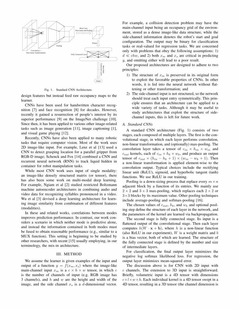
Fig. 1. Standard CNN Architecture.

design features but instead feed raw occupancy maps to thelearner.

CNNs have been used for handwritten character recog-nition [7] and face recognition [8] for decades. However,recently it gained a resurrection of people’s interest by itssuperior performance [9] on the ImageNet challenge [10].Since then, it has been applied to various other image-relatedtasks such as image generation [11], image captioning [1],and visual game playing [12].

Recently, CNNs have also been applied to many robotictasks that require computer vision. Most of the work uses2D image-like input. For example, Lenz et al [13] used aCNN to detect grasping location for a parallel gripper fromRGB-D image; Schenck and Fox [14] combined a CNN andrecurrent neural network (RNN) to track liquid hidden incontainer for robot manipulation tasks.

While most CNN work uses input of single modality:an image-like densely structured matrix (or tensor), therehas also been some work on multi-modal deep learning.For example, Ngiam et al [2] studied restricted Boltzmannmachine autoencoder architectures in combining audio andvideo data for recognizing syllables pronounced in a video.Wu et al [3] devised a deep learning architecture for learn-ing image similarity from combination of different features(modalities).

In these and related works, correlations between modesimproves prediction performance. In contrast, our work con-siders a scenario in which neither mode is predictive alone,and instead the information contained in both modes mustbe fused to obtain reasonable performance (e.g., similar to aMUX function). This setting is beginning to be studied byother researchers, with recent [15] usually employing, in ourterminology, the mix-in architecture.

III. METHOD

We assume the learner is given examples of the input andoutput of a function y = f(xm, xs) where the image-likemain-channel input xm is a c × h × w tensor, in which cis the number of channels of input (e.g. RGB image has3 channels), and h and w are the height and width of theimage, and the side channel xs is a d-dimensional vector.

For example, a collision detection problem may have themain-channel input being an occupancy grid of the environ-ment, stored as a dense image-like data structure, while theside-channel information denotes the robot’s start and goalconfiguration. The output may be binary for classificationtasks or real-valued for regression tasks. We are concernedonly with problems that obey the following assumptions: 1)d � chw, and 2) both xm and xs are critical in predictingy, and omitting either will lead to a poor result.

Our proposed architectures are designed to adhere to twoprinciples:

1) The structure of xm is preserved in its original formto exploit the favorable properties of CNNs. In otherwords, it is fed into the neural network without flat-tening or other transformation; and

2) The side-channel input is not structured, so the networkshould treat each input entry symmetrically. This prin-ciple ensures that an architecture can be applied to awide variety of tasks. Although it may be useful tostudy architectures that exploit the structure of side-channel inputs, this is left for future work.

A. Standard CNNs

A standard CNN architecture (Fig. 1) consists of twostages, each composed of multiple layers. The first is the con-volutional stage, in which each layer performs convolution,non-linear transformation, and (optionally) max-pooling. Theconvolution layer takes a tensor of cin × hin × win andcout kernels, each of cin × hk ×wk, and produce an outputtensor of cout × (hin − hk + 1) × (win − wk + 1). Thena non-linear transformation is applied element-wise to theconvolution output. Typical choices include the rectifyinglinear unit (ReLU), sigmoid, and hyperbolic tangent (tanh)functions. We use ReLU in our training.

Pooling is a down-sizing process that replace every m×nadjacent block by a function of its entries. We mainly use2× 2 and 3× 3 max-pooling, which replaces each 2× 2 or3×3 blocks by its maximum value. Other pooling techniquesinclude average-pooling and softmax-pooling [16].

The chosen values of cout, hk, and wk and optional pool-ing step define the structure of each layer in the network, andthe parameters of the kernel are learned via backpropagation.

The second stage is fully connected stage. Its input is aflattened output of the convolutional stage. Then each layercomputes h(W · x + b), where h is a non-linear function(also ReLU in our experiment), W is a weight matrix and bis a bias vector, both of which are learned. The structure ofthe fully connected stage is defined by the number and sizeof intermediate layers.

For classification, the final output layer minimizes thenegative log softmax likelihood loss. For regression, theoutput layer minimizes mean-squared error.

The discussion above is for CNN with 2D input withc channels. The extension to 3D input is straightforward.Briefly, volumetric input is a 4D tensor with dimensionsc×l×w×h. Each individual kernel is a 4D tensor swept in a4D tensor, resulting in a 3D tensor (the channel dimension is

…

…

…

reshape

⨀

element-wise product activated input

activated map

main-channel

fully-connected network

CN

N

side-c

han

nel

Fig. 2. Activation Map Architecture.

collapsed because it is not swept across). Pooling is modifiedto operate on a cuboid for each channel.

B. Activation Map

The activation map architecture (Fig. 2) makes the as-sumption that the side-channel information “modulates” themain input in a clearly hierarchical way in that the relevanceand usage of main input is determined by the side-channelinformation.

It is structured to first build an “activation map” which hasthe same dimensions as the main-channel input. This stageuses a fully connected deep network to learn a transformationfrom xs to an “activation list” of length c · h · w, which isthen reshaped to a w × h× c activation map. The element-wise product of the activation map and main-channel inputis then fed into a standard CNN to produce the output.

C. Mix-In

The mix-in architecture (Fig. 3) has a standard CNNstructure in the convolutional stage and uses only the main-channel input. Immediately after the convolutional stage, theside-channel information is mixed into the flattened neuronsand propagates through the fully-connected stage.

D. Stacking

The stacking architecture (Fig. 4) augments the main-channel input by stacking it with d layers of side-channelinput, in which d is the dimension of side-channel informa-tion. Each layer contains replicated values of xs for eachelement of xm, and there are as many new layers as numberof side-channel input sources. Thus, if side-channel sourcescontain 4 numbers denoting the 2D start and goal position,and the main-channel input is a 1× h× w occupancy grid,then the augmented input is of size 5× h× w.

main-channel

Convolutional

Stage

flattened

convo

lutio

n o

utp

ut

side- channel

Fully-connected Stage

Fig. 3. Mix-In Architecture

kernel

side-channel

main-channel replicate

CNN

Fig. 4. Stacking Architecture

E. Input-Modulated Kernel

The input-modulated kernel architecture (Fig. 5) uses side-channel information to determine the kernel weights usedfor convolution. For each layer in the convolutional stage, afully-connected network maps the side-channel input to thekernel weights. Each kernel is computed from an independentfully-connected network.

F. Training and Implementational Details

To train our model, we use the mini-batch-based ADAMoptimization algorithm [17] in all examples, and the batchsize is selected from 5 to 200 so that the GPU memoryis not exhausted (and thus 3D tasks have smaller batchsize). We use the Python package Theano [18] to implementour architectures, which uses NVIDIA CUDA Deep NeuralNetwork library (cuDNN) to perform feedforward and back-propagation of convolution operations. Most of the criticalcomputation jobs are done on a NVIDIA GeForce GTX970with 4GB memory.

IV. TEST PROBLEMS

We designed several toy collision prediction problems sothat each architecture can be tested on an “idealized” domainwhere exact ground truth is available and millions of exam-ples are available for training. Motion feasibility predictioncan serve as a primitive operation in motion planners (e.g.collision detection along a line is needed for tree growth

main-channel

side- channel

…

…

…

fully-connected network

…

side- channel

…

…

…

fully-connected network

Fully-connected Stage

Fig. 5. Input-Modulated Kernel Architecture

Problem MC SC Type Architecture

2D Block 20× 20 4Classification

C3/50-M2-C4/30-M2-F100-F100

2D Indep 20× 20 43D Block 20× 20× 20 6

Simulation 100× 100 4 ClassificationC15/50-M2-C14/30-M3-

C5/20-M2-F100-F100

Col 2D F 100× 100 2Regression

C7/50-M2-C6/50-M2-C4/50-M2-F1000-F100Col 2D V 100× 100 4

Col Arm 52× 52× 34 1 RegressionC3/50-M2-C(2,2,3)/50-M2-C(3,3,2)/50-C3/50-

F1000-F500

TABLE ISUMMARY OF TEST PROBLEMS. MC MEANS MAIN-CHANNEL

DIMENSION; SC MEANS SIDE-CHANNEL DIMENSION.

in RRT), and collision distance/time prediction are requiredof autonomous vehicle navigation and safety in industrialrobotic assembly. Table I summarizes key parameters ofeach problem. All main-channel inputs are in the form ofan occupancy grid.

For the architecture column, “Cx/y” means a convolutionlayer of with y kernels each of size x, which is a scalargiving side length for equilateral kernel or a tuple givingkernel shape; “Mx” a means max-pooling layer with down-sampling rate of x on each side; “Fx” means a fully-connected layer with x output variables. The output layer isnot specified as its shape is fully determined by the numberof output variables of the second-to-last layer.

a) Straight-line collision prediction: In 2D Block, 2DIndep, and 3D Block, the task to learn is whether a linesegment is collision-free in a grid of obstacles. The side-channel information is the start and end of the segment,comprising 4 numbers in 2D and 6 numbers in 3D. For the2D cases, start positions and goal positions are randomly

Fig. 6. 2D Block and 2D Indep collision prediction problems: Blackdenotes obstacles.

Fig. 7. Simulation problem: the prediction is whether a point mass slidingalong obstacles can reach the goal, or settles into a local minimum (blackis free and white is obstacles)

selected within the workspace, while for the 3D case, theyare selected from top and bottom face respectively. In 2DBlock and 3D Block, obstacles are sampled as randomrectangles/cuboids, while in 2D Indep, occupied grid cellsare sampled independently at random (Fig. 6).

b) Simulation Connectivity Prediction: In Simulation,the task is to predict whether a point mass can move to agoal using gradient descent (Fig. 7). Start and goal positionsare generated uniformly at random and random trianglesobstacles are generated. Then, a physics simulation is runto move a point mass from start position to goal position,assuming obstacles are fixed and frictionless. The point canslide against obstacles and still reach the goal configuration,or it could be caught in a local minimum.

c) 2D Collision Distance/Time Prediction: In Col 2D,the task is to predict the time at which a point mass, movingin a 2D workspace, would collide with obstacles. Randomdisk obstacles are scattered in the workspace. Two variationsof the problem are considered.

1) Fixed Path (Col 2D F): The robot moves on a fixed pathwith uniform speed (Fig. 8 (a)). The side-channel inputis the current (x, y) position of the robot. Our trainingand testing sets only maintain obstacle configurationsthat at least collide with part of the robot path.

2) Variable Path (Col 2D V): The robot moves in arandom direction with a uniform speed. The side-

channel input is four numbers (x, y, vx, vy) denotingcurrent position and velocity with vx, vy ∈ ±[1, 5]. Theoutput is the time to nearest collision.

In both cases, the distance to nearest collision is calculatedby simple geometry.

(a) Col 2D F (b) Col Arm

Fig. 8. Col 2D F and Col Arm problem: path is traced out in red.

d) Arm Collision Distance Prediction: In Col Arm thetask is similar to Col 2D Fixed Path, but rather than usinga point mass robot, a 3D industrial robot model (StaubliTX90L) is used (Fig. 8 (b)). The robot moves along afixed path that spans much of its workspace. The obstaclesare approximately human-sized cylinders simulating humanswalking around the robot. The robot is also included in theoccupancy grid, as though it were sensed by cameras.

The robot path is discretized to 4726 steps such thatconsecutive configurations have very similar but differentoccupancy grid. The side-channel is simply the index of theconfiguration. The output to be learned is the number of stepsuntil first collision with an obstacles.

V. RESULTS

A. Summary

Table II shows the testing performance for each archi-tecture on each task, reporting error rate for classificationproblems and root-mean-squared error for regression. Duringtesting, a random subset of a pool of test problems is selectedand error is measured. Then we smooth the test error acrossiteration using moving average, and the number to averageis much less than total number of test iterations so that theinitial high error stage does not affect the final test result.The Base column displays error of a baseline CNN trainedonly on main-channel input. The Range column shows theminimum and maximum possible error. The Kernel architec-ture trained extremely slowly, and after a day of training timewith no sign of convergence, we marked results with T!. For3D Block and Col 2D V, stacking side-channel input to theoriginal main-channel input will exceed the 4GB memoryon the GPU. For these tasks (denoted with *) we stack theside-channel with the output of the first max-pooling layer.

B. Typical results

A typical learning curve is shown on 2D Block (Fig. 9).Two activation map parameters are tested, with X hiddenneurons per layer in the activation stage (Activation X).

Act Mix-In Stack Kernel Base Range

2D Block 1.7% 5.8% 3.8% 4.6% 27.2% [0, 100%]2D Indep 6.8% 22.6% 18.3% T! 33.8% [0, 100%]3D Block 4.4% 5.4% 4.7%∗ T! 25.2% [0, 100%]Simulation 23.9% 26.8% 35.0% T! 47.0% [0, 100%]Col 2D F 16.8 14.8 19.5 T! 72.2 [0, 331]Col 2D V 2.20 2.82 2.25∗ T! 5.72 [0, 100]Col Arm 84 139 280 T! 104 [0, 4725]

TABLE IIERRORS OF EACH ARCHITECTURE ON VARIOUS TASKS. “ACT” COLUMN

REPORTS BEST PERFORMANCE AMONG 3 PARAMETER SETTINGS. “T!”MEANS TRAINING TIME IS TOO LONG TO REACH CONVERGENCE. “*”INDICATES THAT, DUE TO MEMORY ISSUES, THE SIDE-CHANNEL WAS

STACKED TO THE OUTPUT OF THE FIRST MAX-POOLING LAYER RATHER

THAN THE MAIN CHANNEL.

Fig. 9. Typical learning curves, here shown for 2D Block. (Best viewedin color)

Activation 1000 performs best, followed by stack, mix-in, kernel (stopped at around 2000th iteration due to slowtraining), and Activation 10.

For the 2D Col F regression problem, Fig. 10 plotsground truth vs. prediction for each test instance and acumulative distribution function (CDF) of error for the mix-in architecture, which performed the best on this task. Theprediction is generally close to ground-truth, with 95% oferrors less than 28.2 units (<10% of output range).

We can visualize the effect of side-channel informationin several ways. For the activation map architecture, themap can directly reveal how side-channel information is

(a) Ground truth vs. prediction (b) CDF of errors

Fig. 10. Mix-in architecture test results on Col 2D. (Best viewed in color)

Fig. 11. Activation maps for certain start and end points (indicated ascircles) for collision prediction problems. Warmer color indicates higheractivation. Left: 2D Blocks. Middle: 3D Block. Right: 500 largest values ofthe same 3D Block example. (Best viewed in color)

Fig. 12. Activation map for Simulation problem: The activation pattern isnot as distinct as collision prediction, because the existence of an obstaclecan “steer away” a path from a straight line. (Best viewed in color)

incorporated into the prediction. In collision detection tasks,the learned activation map approximates the swept volumeof the robot (Fig. 11). However, it is less interpretable on theSimulation problem (Fig. 12) where relevance is intimatelytied with the main-channel input.

C. Interpretation

In general, we observe the following trends.1) Activation map performs well all around, but works

best when side-channel input solely and uniquely de-termines the relevance of main-channel input;

2) Mix-in is good when the main-channel input also af-fects the relevance of itself but may suffer from loss ofinformation due to over-compression in convolutionalstage;

3) Stacking generally does not perform as well and scalespoorly with the number of side-channel inputs d; and

4) Input-modulated kernel takes too long for evenmoderately-sized problems, and thus is not practical.

5) Baseline CNNs are usually unable to achieve goodperformance. The exception is when the side-channelinformation is “naturally” included in the main-channelinformation, as observed in the Col Arm task.

The advantages and disadvantages of each architecture arediscussed in more detail below.

a) Activation Map: Besides its good performance, anadvantage of the activation map is that it is highly inter-pretable via visualization. It also performs the best whenthe side-channel input can by itself determine the relevanceof main-channel input, e.g., in collision detection where

(a) Activation 10 (b) Activation 1000 (c) Activation 2000

Fig. 13. Effect of the number of neurons per hidden layer for activationmap. For 2D Indep, (a) 10 neurons are not expressive enough to representthe straight-line swept volume, (b) 1000 neurons per hidden layer gives bestperformance, and (c) 2000 neurons overfit the training examples, exhibitingactivation in the lower right region of the environment regardless of startand goal positions. (Best viewed in color)

Fig. 14. Activation map for fixed-path 2D collision time prediction task.The entire path is activated because side-channel information alone cannotuniquely determine the relevance of features. Robot current position iscircled in red. (Best viewed in color)

the activation approximates the swept volume (Fig. 11).It performs worse (but still fairly well) on the simulationfeasibility problem (Fig. 12) where relevance is intimatelytied with the main-channel input. Similarly, for collisiontime prediction (Fig. 14), it predicts that the whole pathis potentially relevant, but an even more minimal activationmap could be determined by the order of configurations onthe path: if an obstacle appears early on the path, then theremainder is actually irrelevant.

There are two main disadvantages of the activation map.First, its performance is relatively sensitive to the chosennumber of neurons in the activation stage. Second, the mapis computed through a fully-connected network and requiresmany hidden neurons per intermediate layer (Fig. 13) toinduce a flexible-enough function. However, since the num-ber of main-channel inputs is large, learning such a fully-connected network may require a lot of data and be proneto over-fitting (note the extraneous pattern on Fig. 14).

b) Mix-In: Mix-in offers the best space efficiency andno tuning requirement, and performs reasonably well. Theconvolutional stage acts as a feature detector that compressesmain-channel input down to a small set of features, whichmay destroy important information that should be mixed

with the side-channel input. For example, in 2D Indep, theenvironmental variation is quite large, and it is hard for acompressed representation to capture all subtleties of theoriginal environment.

c) Stacking: Space complexity is the biggest problemwith stacking, in that it augments the initial O(chw + d)input to O((c+d)hw). It also appears to have poor capacityand/or fall into local minima, performing quite poorly on the2D Indep, Simulation, and Col Arm examples.

d) Kernel: Training of the input-modulated kernel ar-chitecture is prohibitively expensive even for moderatelysized problems, and thus its characteristics are not fullystudied. The cuDNN library is optimized for computingsimultaneous convolution of multiple images with the samekernel. In this architecture, each kernel is dependent on side-channel information, which is different for each trainingexample. Thus, batch-based training cannot be performed inparallel.

VI. CONCLUSION

This paper empirically compared four candidate architec-tures for incorporating side-channel information into CNNs.Experiments on simulated collision prediction problems sug-gests that the Activation Map architecture, which maps theside-channel to a pixel-by-pixel modulation of the image-like main-channel, generally performs well. However, itsperformance is sensitive to the tuning of the number ofneurons per layer, and may be susceptible to overfitting inthe presence of huge numbers of main-channel inputs due tothe use of fully-connected networks.

To address this latter problem it may be possible to borrowthe idea of local receptive field of CNNs, in which spatialcoherence is used to gradually reduce the size of the inputdata. In our case, we can “reverse” the process to graduallybuild larger and larger maps, until the map has the same sizeas the main-channel input. This idea makes sense intuitivelybecause an activation map is also likely to exhibit spatialcoherence much like the main-channel (i.e. if one positionis relevant, its neighbors tend also to be relevant).

More study is needed to assess the quality of the Kernelarchitecture, which is currently impractical on large problemsdue to the inability to perform batch convolution. New soft-ware and/or hardware support of fast individual convolutionshould be developed to study this idea further. It may bealso possible to improve prediction performance even furtherwith hybrid network structures, such as activation + mix-in.In addition, a more compact stacking layer could be learnedfrom a fully connected network (similar to the activationarchitecture) and stacked to augment the main-channel input.

REFERENCES

[1] A. Karpathy and L. Fei-Fei, “Deep visual-semantic alignments forgenerating image descriptions,” in Proc. IEEE Conf. Computer Visionand Pattern Recognition (CVPR), 2015, pp. 3128–3137.

[2] J. Ngiam, A. Khosla, M. Kim, J. Nam, H. Lee, and A. Y. Ng,“Multimodal deep learning,” in Proc. 28th Intl. Conf. on MachineLearning (ICML), 2011, pp. 689–696.

[3] P. Wu, S. C. Hoi, H. Xia, P. Zhao, D. Wang, and C. Miao, “Online mul-timodal deep similarity learning with application to image retrieval,”in Proc. 21st ACM Intl. Conf. Multimedia, ser. MM ’13. New York,NY, USA: ACM, 2013, pp. 153–162.

[4] J. Pan, S. Chitta, and D. Manocha, “Faster sample-based motionplanning using instance-based learning,” in Algorithmic Foundationsof Robotics X. Springer, 2013, pp. 381–396.

[5] N. Jetchev and M. Toussaint, “Trajectory prediction: learning tomap situations to robot trajectories,” in Proc. 26th Annual Int. Conf.Machine Learning (ICML). ACM, 2009, pp. 449–456.

[6] ——, “Trajectory prediction in cluttered voxel environments,” in Proc.IEEE Intl. Conf. Robotics and Automation (ICRA). IEEE, 2010, pp.2523–2528.

[7] Y. LeCun, L. Bottou, Y. Bengio, and P. Haffner, “Gradient-basedlearning applied to document recognition,” Proc. IEEE, vol. 86, no. 11,pp. 2278–2324, 1998.

[8] S. Lawrence, C. L. Giles, A. C. Tsoi, and A. D. Back, “Facerecognition: A convolutional neural-network approach,” IEEE Trans.Neural Networks, vol. 8, no. 1, pp. 98–113, 1997.

[9] A. Krizhevsky, I. Sutskever, and G. E. Hinton, “Imagenet classificationwith deep convolutional neural networks,” in Advances in NeuralInformation Processing Systems (NIPS), 2012, pp. 1097–1105.

[10] J. Deng, W. Dong, R. Socher, L.-J. Li, K. Li, and L. Fei-Fei,“Imagenet: A large-scale hierarchical image database,” in Proc. IEEEConf. Computer Vision and Pattern Recognition (CVPR), 2009, pp.248–255.

[11] K. Gregor, I. Danihelka, A. Graves, D. J. Rezende, and D. Wier-stra, “Draw: A recurrent neural network for image generation,”arXiv:1502.04623, 2015.

[12] V. Mnih, K. Kavukcuoglu, D. Silver, A. A. Rusu, J. Veness, M. G.Bellemare, A. Graves, M. Riedmiller, A. K. Fidjeland, G. Ostrovskiet al., “Human-level control through deep reinforcement learning,”Nature, vol. 518, no. 7540, pp. 529–533, 2015.

[13] I. Lenz, H. Lee, and A. Saxena, “Deep learning for detecting roboticgrasps,” Intl. J. Robotics Research (IJRR), vol. 34, no. 4-5, pp. 705–724, 2015.

[14] C. Schenck and D. Fox, “Detection and tracking of liquids withfully convolutional networks,” in Proc. Robotics: Science and SystemsWorkshop on Are the Sceptics Right? Limits and Potentials of DeepLearning in Robotics, 2015.

[15] S. Levine, C. Finn, T. Darrell, and P. Abbeel, “End-to-end trainingof deep visuomotor policies,” J. Machine Learning Research (JMLR),vol. 17, no. 39, pp. 1–40, 2016.

[16] O. Abdel-Hamid, L. Deng, and D. Yu, “Exploring convolutionalneural network structures and optimization techniques for speechrecognition,” in Proc. Interspeech Conference, 2013, pp. 3366–3370.

[17] D. Kingma and J. Ba, “Adam: A method for stochastic optimization,”arXiv:1412.6980, 2014.

[18] Theano Development Team, “Theano: A Python frameworkfor fast computation of mathematical expressions,” arXiv,vol. abs/1605.02688, May 2016. [Online]. Available: http://arxiv.org/abs/1605.02688