incorporating bayesian analysis to improve the accuracy of...
TRANSCRIPT

1
Incorporating Bayesian Analysis to Improve the Accuracy ofCOCOMO II and Its Quality Model Extension
by
Sunita Devnani-Chulani
University of Southern CaliforniaCenter for Software EngineeringComputer Science Department

2
Outline
1. Introduction ………………………………………………………………..…….1
2. Evaluating Existing Software Estimation Techniques …………………..……32.1 Model-Based 32.2 Expertise-Based 102.3 Learning-Oriented 102.4 Dynamics-Based 112.5 Regression-Based 122.6 Composite 13
3. Research Approach……………………………………………………..………153.1 The seven-step modeling methodology 153.2 The Bayesian Approach 17
3.2.1 A Simple Software Cost Estimation Model3.2.2 Incorporating the modeling methodology for COCOMO II
3.3 A-Priori Cost/Quality Model 283.3.1 Defect Introduction Model3.3.2 Data Collection
4. Status and Plans……………………………………………………..……….…394.1 COCOMO II.1997 Calibration 394.2 COCOMO II Bayesian Prototype 454.3 Quality Model Current Research Results 49
5. References……………………………………………………..………………...53
6. Appendices……………………………………………………..………………..55A COCOMO II Cost Estimation Questionnaire 55B COCOMO II Delphi Questionnaire 80C Defect Introduction Model Behavioral Analysis and Results of Two-Round Delphi 97D Defect Removal: Model Behavioral Analysis 123

1
Chapter 1: Introduction
Large scale software development management and control requires the use of quantitative softwareestimation and assessment models that are based upon theory and collected historical project data. Dozensof models have been developed in the last two decades that predict software cost and schedule at an earlystage of the development life cycle, i.e. soon after the requirements have been established. These estimatesare used to manage the software development process in the hope of delivering the software product ontime, within budget and with the expected quality. In spite of the plethora of these models, most softwaredevelopment projects experience large schedule and cost overruns. One reason for this is that the existingcost models are insufficient and do not yield accurate estimates. With the increase in the ratio of softwarecosts over hardware costs [Boehm81]; a big challenge in software engineering has been to accuratelypredict software costs.
Several studies [Kemerer87, Stukes94] have compared two or more existing cost models. The results ofthese studies usually exhibit dissatisfaction in the accuracies of these models and conclude that localcalibration needs to be performed to improve predictability. Most of these models are proprietary (SPR’sCheckpoint[Jones97], Price-S[Park88], Jensen’s model [Jensen84], Estimacs[Rubin83] etc.). Whereas afew other models (COCOMO[Boehm81, CSE1], Softcost[Tausworthe81], Bailey-Basili’s Meta-model[Bailey81]) are available in the public domain. Of these published models, COCOMO has been verywidely used and accepted. It has been publicly available since 1981 and many commercial vendors havedeveloped tools (CoCoPro, CB COCOMO, COCOMOID, Costar, COSTMODL, GECOMO Plus, GHLCOCOMO SECOMO, SWAN, etc.) to support the COCOMO model equations. Several researchers[Gulezian86, REVIC88] have taken the published COCOMO form and developed their own models. Forthe purpose of this research also, COCOMO was the strongest candidate.
The earliest published version of COCOMO is the COCOMO ’81 version. It was developed by BarryBoehm at TRW and had three levels of increasing detail and accuracy; Basic; Intermediate and Detailed.The most popular Intermediate COCOMO ’81 gives estimates that are within 20% of the actuals 68% of thetime. COCOMO ’81 has been widely used since the early 80s. The Ada COCOMO model was developed inthe late 1980s to address the need for a cost model for Ada projects. Both these models have experienceddifficulties in estimating software projects of the 90s due to challenges such as non-sequential and rapid-development process models; reuse-driven approaches involving commercial-off-the-shelf (COTS)packages, reengineering, applications composition, and application generation capabilities; object-orientedapproaches supported by distributed middleware; software process maturity effects and process-drivenquality estimation. To meet these changing needs, the COCOMO II research effort was initiated in 1994[Boehm95]. The first calibrated version, COCOMO II.1997 gives estimates that are within 20% of theactuals 46% of the time. Comparing the COCOMO ’81 model with the COCOMO II.1997 model revealsthat the COCOMO II.1997 model when used on software projects developed in the late 1980s and the1990s yields lower accuracies versus the COCOMO ’81 model when used on software projects developedin the 1970s and the early 1980s. This appears to be due partly to lack of dispersion for some variables;imprecision of software effort, schedule, and cost driver data; and effects of partially correlated variables.But the major difference is most likely the change from a uniform waterfall-model sample of projects inCOCOMO ’81 versus a wide variety of project types in the COCOMO II calibration sample.
The COCOMO II.1997 model was calibrated on a dataset of 83 projects using multiple regression analysis.This technique is well-suited when(i) a lot of data is available. This indicates that there are many degrees of freedom available and the
number of observations is many more than the number of variables to be predicted. Collecting data hasbeen one of the biggest challenges in this field due to lack of funding by higher management, co-existence of several development processes, lack of proper interpretation of the process, etc.
(ii) no data items are missing. Data with missing information could be reported when there is limited timeand budget for the data collection activity; or due to lack of understanding of the data being reported.
2
(iii) there are no outliers. Extreme cases are very often reported in software engineering data due tomisunderstandings or lack of precision in the data collection process, or due to different “development”processes.
(iv) the predictor variables are not correlated i.e. there is minimal heteroscedasticity. Most of the existingsoftware estimation models have parameters that are correlated to each other. This violates theassumption of the OLS approach.
(v) the predictor variables have an easy interpretation when used in the model. This is very difficult toachieve because it is not easy to make valid assumptions about the form of the functional relationshipsbetween predictors and their distributions.
(vi) the regressors are either all continuous (e.g. Personnel capability) or all discrete variables (Defectdensity). Several statistical techniques exist to address each of these kind of variables but not both inthe same model.
Each of the above six restrictions are violated to various extents by software engineering data. Hence, thereis a need for a more sophisticated approach to analyzing the data and developing a better cost model. Thefocus of this research is the Bayesian approach to data analysis and model building. It does not solve all theproblems faced by multiple regression analysis but alleviates a few of them; namely the problems of scarcityof software effort data, missing data on reported datapoints and outliers. The aim of this proposal is topresent the Bayesian approach and to show that it can be used on available software engineering effort,schedule and quality data. The important question that will be answered by the thesis which will be thecompletion of this research is: “Does Bayesian analysis improve the accuracy of the COCOMO modelversus multiple regression analysis?” In the process of answering this question, a 7-step methodology forbuilding software estimation models will be developed. This methodology will be used to develop thecomplete Quality Model extension to COCOMO II.

Evaluating Existing Software Estimation Techniques 3
Chapter 2: Evaluating Existing Software Estimation Techniques
Software development costs continue to increase and practitioners continually express their concerns overtheir inability to accurately predict the costs involved. One of the most important objectives of the softwareengineering community has been the development of useful models that constructively explain thedevelopment life cycle and accurately predict the cost of developing a software product. Many softwareestimation models have evolved in the last two decades based on several different model buildingtechniques. Classical techniques (such as Regression analysis) are not the best for software engineeringdata. Several papers discuss the [Briand92, Khoshgoftaar95] pros and cons of one technique versus anotherand present data analysis results. This section focuses on the classification of existing techniques into sixmajor categories as shown in figure 2.1.
2.1 Model-Based Techniques
Many software estimation models have been developed in the last two decades. Many of them areproprietary models and hence cannot be compared and contrasted in terms of the model structure and howmuch of prior knowledge v/s data-determined information is driving the model parameters. Theory orexperimentation determines the functional form of these models. This section discusses a few of the popularmodels and focuses on the predictor variables that are used to develop the models. Wherever appropriate, adiscussion of the quality model is also included. After significant amount of research the author concludedthat other than Bailey-Basili’s meta-model [Bailey81], Gulezian’s model [Gulezian 86] and the COCOMOmodels [Boehm81, Boehm95, CSE1] none of the other models present statistical results which recognizeand quantify the individual factors influencing productivity or quality.
Putnam’s Software Life Cycle ModelLarry Putnam of Quantitative Software Measurement developed the Software Life Cycle Model (SLIM) inthe late 1970s [Putnam92]. SLIM is based on Putnam’s analysis of the life-cycle in terms of a Rayleighdistribution of project level personnel level versus time. It depends on a SLOC (Source Lines of Code)estimate for the size of the project and then alters this through the use of a Rayleigh curve to estimateproject effort, schedule and defect rate. The Manpower Buildup Index (MBI) and a Technology Constant orProductivity factor (PF) can be used to influence the shape of the curve. SLIM can record and analyze datafrom previously completed projects which is then used to calibrate the model; or if data is not available thena set of questions can be answered to get values of MBI and PF from the existing database.
In SLIM, Productivity is used to link the basic Rayleigh manpower distribution model to the softwaredevelopment characteristics of size and technology factors. Productivity, P, is the ratio of software productsize, S, and development effort, E. That is,
PS
E= Eq.2.1
The Rayleigh curve used to define the distribution of effort is modeled by the differential equation
Figure 2.1: Software Estimation Techniques
Software Estimation Techniques
Model-Based -
SLIM, COCOMORegression-Based -
OLS, RobustDynamics-Based
Learning-Oriented -
Neural, Case-based
Expertise-Based -
Delphi, WBS
Composite -
Bayesian
Evaluating Existing Software Estimation Techniques 4
dy
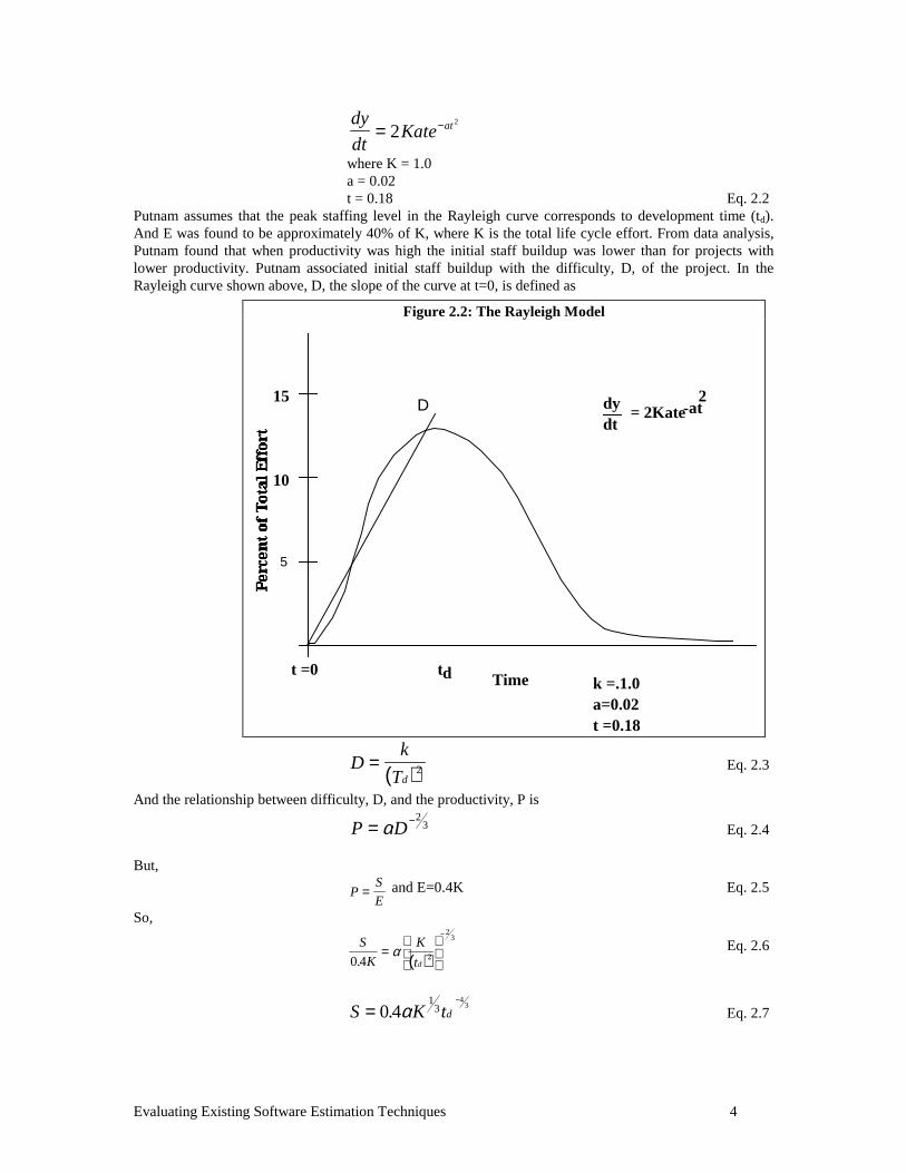
dtKate at= −2
2
where K = 1.0a = 0.02t = 0.18 Eq. 2.2
Putnam assumes that the peak staffing level in the Rayleigh curve corresponds to development time (td).And E was found to be approximately 40% of K, where K is the total life cycle effort. From data analysis,Putnam found that when productivity was high the initial staff buildup was lower than for projects withlower productivity. Putnam associated initial staff buildup with the difficulty, D, of the project. In theRayleigh curve shown above, D, the slope of the curve at t=0, is defined as
( )Dk
Td= 2 Eq. 2.3
And the relationship between difficulty, D, and the productivity, P is
P D= −α2
3 Eq. 2.4
But,
PS
E= and E=0.4K Eq. 2.5
So,
( )S
K
K
td0 4 2
23
.=
−
α Eq. 2.6
S K td=−
0 41
34
3. α Eq. 2.7
Figure 2.2: The Rayleigh Model
15
10
5
t =0
dydt
= 2Kate-at 2D
k =.1.0a=0.02t =0.18
Timetd

Evaluating Existing Software Estimation Techniques 5
Thus, Effort can be formulated as
KS
td
13
430 4
=. ( )α
Eq. 2.8
Putnam suggests 0.4α is a technology factor, C, which accounts for differences among projects and basedon his study he has 20 different values for C ranging from 610 to 57314. This study was not based onexhaustive data analysis and is more theory oriented. Hence,
KS
C td
= ×3
3 4
1 Eq. 2.9
Substituting, E = 0.4K, we get
ES
C td
= ×
×0 413
4. Eq. 2.10
For the Quality model in SLIM, Putnam assumed the Rayleigh Defect Rate curve based on Trachtenburg’sstudy [Trachtenburg82] at RCA in 1982 of more than 25 software reliability models. The Rayleigh equationfor the error curve is modeled as
E E t t t tm r d d= −( / ) exp( / )6 32 2 2 Eq. 2.11
whereEr = Total number of errors expected over the life of the projectEm = Errors per montht = instantaneous elapsed time throughout the life cycletd = elapsed time at milestone 7, the 95% reliability level
Putnam approximated the error curve shown in figure 2.3. Most of the available defect data was inaggregate form; it represented activities from system integration test to product delivery (i.e. the end ofdevelopment). Putnam integrated the area under the Rayliegh curve and realized that these activitiescomprised 17% of the total area. He used this result to compute the total number of defects under the curve.Thus a flaw of Putnam’s Defect model (like many of the Reliability models that Trachtenburg studied) isthat it uses data known only after testing begins.
Jensen Model
Figure 2.3: The Trachtenburg Reliability Rayleigh Curve
0
25
50
75
100
125
150
175
200
225
250
0 1 2 3 4 5 6 7 8
Time(t)
Defects Over Time

Evaluating Existing Software Estimation Techniques 6
The Jensen model [Jensen84] is very similar to the Putnam SLIM model described above. He proposed
S C TKte=1
2 Eq. 2.12
where
ES
C Tte=
×0 4
12
2. Eq. 2.13
Jensen’s Effective Technology Constant, Cte, is a slight variation of Putnam’s technology factor, C. Jensen’sCte is a product of a basic technology constant and several adjustment factors (similar to the IntermediateCOCOMO ‘81 form of Effort Adjustment Factor). The adjustment factors account for differences inproduct, personnel and computer factors among different software products.
Bailey-Basili’s ModelJohn Bailey and Vic Basili [Bailey81] attempted to present a model generation process for developing alocal resource estimation model. The process consists of 3 steps(i) Compute background equation(ii) Determine factors explaining the differences between actual project data and the mean of the estimated
derived by the background equation.(iii) Use model to predict new project.
The background equation or the baseline relationship between effort and size was determined using 18datapoints from the NASA SEL (Software Engineering Lab) database. It was formulated as
Effort (in Man Months) = 0.73 (Size in Delivered SLOC)1.16 + 3.5 Eq. 2.14
This equation can be used to predict the effort (standard effort or nominal effort) required to complete anaverage project.
The next step in the process is to determine a set of factors that differentiates one project from another andhelps explain the difference between actual effort v/s effort estimated by the background equation. Baileyand Basili identified close to 100 environmental attributes as possible contributors to the variance in thepredicted effort. They also noted that using so many attributes with only 18 data points was not feasible andidentified techniques of selecting only the most influential ones. They recognized that determining a subsetof the attributes can be done by expert intuition, factor analysis or by the use of correlation matrices. Theyalso grouped attributes in a logical way so that the group had either a positive or a negative impact on effortand could be easily explained. They finally settled upon 3 groups using only 21 of the original attributes.The groups are
Total Methodology (METH)Tree ChartsTop Down DesignDesign FormalismsCode ReadingChief Programmer TeamsFormal Test PlansUnit Development FoldersFormal Training
Cumulative Complexity (CMPLX)Customer Interface ComplexityCustomer-Initiated Design ChangesApplication Process ComplexityProgram Flow ComplexityInternal Communication ComplexityExternal Communication ComplexityData Base Complexity

Evaluating Existing Software Estimation Techniques 7
Cumulative Experience (CEXP)Programmer QualificationsProgrammer Experience with Machine
Programmer Experience with LanguageProgrammer Experience with ApplicationTeam Previously Worked Together
Each of these groups was rated on a scale from 1 to 5 and then SPSS was used to run multiple regression onthe several combinations of the attributes such as
Effort = (Size)A * METH
Effort = (Size)A * METH*CMPLX
Effort = (Size)A * METH*CMPLX*CEXP
Bailey and Basili concluded that none of the model types they investigated was better than the rest. As moredata is available the model structures should be further investigated and the model with highest predictionaccuracy should be determined. This model can then be used for predicting a new project.
COCOMOThe recently published COCOMO II model [Boehm95, CSE1] was preceded by the original COCOMO ’81model published in [Boehm81]. The COCOMO ’81 model has 3 levels of increasing detail and accuracy;Basic; Intermediate and Detailed. The top-level Basic COCOMO model is good for quick, early, rough-order of magnitude estimates of software costs. It models Effort as a non-linear function of Size as shown inEquation 1.
[ ]Effort A SizeB
= × Eq. 2.15
The next level of detail is the Intermediate COCOMO model (Equation 2.1.16); which formulates Effort asa function of Size and a set of Effort Multipliers which account for differences in hardware constraints,personnel quality and experience, use of modern tools and techniques, and other significant parameters. Thethird level of COCOMO ’81 is the Detailed COCOMO which accounts for the effect of these parameters onthe different phases.
[ ]Effort A Size EffortMultiplierB
ii
= × ×=
∏1
15
Eq. 2.16
The COCOMO II research effort started in 1994 and its initial definition and rationale are described in[Boehm95]. COCOMO II has a tailorable mix of three models, Applications Composition; Early Design;Post-Architecture, which target the realm of future software practices marketplace. The Post-Architecturemodel which is the most mature of these 3 submodels has been calibrated to a set of 83 datapoints[Chulani97A].
The Post-Architecture model, as the name suggests, is typically used after the software architecture is welldefined and established. It estimates for the entire development life cycle of the software product and is adetailed extension of the Early-Design model. This model is the closest in structure and formulation to theIntermediate COCOMO ’81 (Equation 2.16) and Ada COCOMO models.
The model uses a set of 17 multiplicative effort multipliers and a set of 5 exponential scale factors to adjustfor project, platform, personnel, and product characteristics. The effort multipliers have a nominal rating of1.0 assigned to them. Depending on the effect the effort multiplier has on effort the value is either greaterthan 1.0 (detrimental effect) or less than 1.0 (reduces development effort). The scale factors determine theeconomies/diseconomies of scale of the software under development replacing the development modes in

Evaluating Existing Software Estimation Techniques 8
the COCOMO ’81 model and refining the exponent in the Ada COCOMO model. For further explanationand comparisons between the various COCOMO models the reader is urged to read [Boehm95]. Amultiplicative constant, A, is used to calibrate the model locally for a better fit and it captures the lineareffects of effort in projects of increasing size. The Post-Architecture model described above has thefollowing form
[ ]Effort A Size EffortMultiplierB
ii
= × ×=
∏1
17
Eq. 2.17
where B ScaleFactorjj
= + ×=
∑1 01 0 011
5
. . and Eq. 2.18
A = Multiplicative ConstantSize = Size of the software project measured in terms of KSLOC (thousands ofSource Lines of Code [Park92], Function Points [IFPUG94] or Object Points[Banker92])
Gulezian’s modelRonald Gulezian developed a methodology for utilizing COCOMO inputs to formulate a generalizedsoftware development cost estimation model [Gulezian86]. He reformulated the original IntermediateCOCOMO ’81 model and showed how multivariate linear regression techniques can be used to determinethe coefficients of each of the parameters to calibrate the COCOMO model locally. The model equation thathe derived was
Effort a Size c destimatedb e
iEffortMultiplier
i
i==
∏( ) ( )mod
1
15
Eq. 2.19
wherea, b = Coefficients of nominal estimating equation for one of the threedevelopment modesc = Coefficient estimate corresponding to mode variabledi = Coefficient estimate corresponding to ith effort multiplier
This equation is transformed using logarithms to achieve a linear equation whose coefficients can beestimated using linear regression techniques.
Hence,
ln( ) (ln ) (ln ) mod (ln ) (ln )Effort a b Size e c EffortMultiplier destimated i ii
= + + +=∑
1
15
ln( ) (ln ) modEffort a b Size c e d EffortMultiplierestimated i ii
= + + +=∑1 1 1
1
15
Eq. 2.20
where a1 = ln a,c1 = ln c andd1 = ln d
Linear regression on this equation yields coefficients and standard errors for each of the parameters. Thelower the standard error the higher is the influence of the parameter on effort. Gulezian also showed howcorrelations between each of the parameters and effort can be determined. Stronger correlations indicatehigher significance of the parameter. In his correlation matrix, (ln Size) and (ln Effortestimated) had acorrelation factor of 0.86 indicating that Size is a very good predictor of development effort.

Evaluating Existing Software Estimation Techniques 9
Many other software estimation models exist but very little about their structure has been published. A shortdescription of a few of these models is presented below.
CheckpointCheckpoint is a knowledge-based software project estimating tool from Software Productivity Research(SPR) developed from Capers Jones’ studies [Jones97]. It has a proprietary database of about 6000software projects and it focuses on four areas that need to be managed to improve software quality andproductivity. It uses Function (or Feature Points) as its primary input of size. SPR’s Summary ofOpportunities for software development is shown in figure 2.4.
Price-SThe Price-S model was initially released in 1977 as a proprietary model. Although most of the equations arenot in the public domain, a few of its central algorithms have been published in [Park88]. Price-S allowsyou to input software size by using SLOC, function point analysis or Sizer, a proprietary technique. Productand process variables are used as input to predict effort and schedule for a given project. A productivityindex using local data points needs to be computed before the tool can be used.
SoftcostThe original SOFTCOST mathematical model was developed for NASA in 1981 by Dr. Robert Tauswortheof JPL [Tausworthe81]. This model has been enhanced using the research results of Boehm, Doty, Putnam,Waltson-Felix and Wolverton. The most debated property of this model is its linear relationship betweeneffort and size. A proprietary set of Softcost-based models (Softcost-R, Softcost-Ada, Softcost-OO) wasalso developed by Reifer Consultants Inc. [Reifer89, Reifer91A, Reifer91B]
EstimacsThe Estimacs model was developed by Howard Rubin of Hunter College in the early 1980s [Rubin83]. Ituses a very similar approach of function points as its size input and estimates effort, staffing requirements,costs and risks involved with a project. The model is now being distributed by Computer AssociatesInternational Inc.
SEER-SEMSEER-SEM is the System Evaluation and Estimation of Resources - Software Estimation model. It isdistributed by Galarath Associates. It uses either lines of code or function points in addition to personnel
Figure 2.4: SPR’s Summary of Opportunities
Software Quality And Productivity
Technology
Environment
PeopleManagement
Developmentprocess
* Establish QA & Measurement Specialists* Increase Project Management Experience
* Develop Measurement Program* Increase JADS & Prototyping* Standardize Use of SDM* Establish QA Programs
* Establish Communication Programs* Improve Physical Office Space* Improve Partnership with Customers
* Develop Tool Strategy

Evaluating Existing Software Estimation Techniques 10
attributes, tools, complexity and constraints as input to estimate cost, schedule, risk and maintenance of asoftware project.
2.2 Expertise-Based Techniques
These software estimation techniques are developed using prior knowledge of experts in the field[Boehm81]. Based on their experience and understanding of the proposed project, experts arrive at anestimate of the cost/schedule. The pros and cons of these techniques are complementary to those of Model-based techniques and are shown in table 1.
Table 1: Pros and Cons of Expertise-Based TechniquesPros Cons
• Easily incorporates knowledge of differencesbetween past project experiences
• No better than the experts
• Assessment of exceptional circumstances,interactions and representativeness
• Estimates can be biased
• Subjective estimates that may not beanalyzable
DelphiThe Delphi technique was originated at The Rand Corporation in 1948 and is an effective way of gettinggroup consensus. It alleviates the problem of individual biases and results in an improved group consensusestimate. As described in [Boehm81], a wideband delphi approach yields better estimates. It is described inTable 2. We have used a slight variation of this approach several times at the Center for SoftwareEngineering’s Focused Workshop [CSE1].
Rule-based systemsThis technique has been adopted from the Artificial Intelligence domain where a known fact fires up ruleswhich in turn may assert new facts. And the system can be used for estimation when no further rules arefired up from known (or new) facts. An example of a rule-based system is shown
If Required Software Reliability = Very High AND Personnel Capability = Lowthen Risk Level = High
Work Breakdown StructuresThis technique of software estimating involves breaking down the product to be developed into smaller andsmaller components until the components can be independently estimated. The estimation can be based onanalogy from an existing database of completed components, or can be estimated by experts, or by using theDelphi technique described above. Once all the components have been estimated, a project-level estimatecan be derived by rolling-up the estimates.
2.3 Learning-Oriented Techniques
Learning-oriented techniques use prior and current knowledge to develop a software estimation model.
Table 2: Wideband Delphi approach1. Coordinator provides Delphi instrument to each of the participants to review.2. Coordinator conducts a group meeting to discuss related issues.3. Participants complete the Delphi forms anonymously and return it to the Coordinator.4. Coordinator feeds back results of participants’ responses.5. Coordinator conducts another group meeting to discuss variances in the participants’’ responses to
achieve a possible consensus.6. Coordinator asks participants for re-estimates, again anonymously, and step 4-6 are repeated for as
many times as appropriate.
Evaluating Existing Software Estimation Techniques 11
Neural NetworksIn the last decade, there has been significant effort put into the research of developing software estimationmodels using neural networks. Many researchers [Khoshgoftaar95] realized the deficiencies of OLSregression methods and explored neural networks as an alternative. Wittig developed a software estimationmodel using connectionist models (synonymous with neural networks as referred in this section) andderived very high prediction accuracies [Wittig94].
Most of the software models developed using neural networks use backpropogation trained feed-forwardnetworks. As discussed in [Gray97], these networks are architected using an appropriate layout of neurons.The network is trained with a series of inputs and the correct output from the training data so as to minimizethe prediction error. Once the training is complete, and the appropriate weights for the network arcs havebeen determined, new inputs can be presented to the network to predict the corresponding estimate of theresponse variable.
Although, Wittig’s model has accuracies within 10% of the actuals, the model has not been well-acceptedby the community due to its lack of explanation. Neural networks operate as ‘black boxes’ and do notprovide any information or reasoning about how the outputs are derived. And since software data is notwell-behaved it is hard to know whether the well known relationships between parameters are satisfied withthe neural network or not. For example, the data in the COCOMO II.1997 database says that developing forreuse causes a decrease in the amount of effort it takes to develop the software product. This is incontradiction to both theory and other data sources [Poulin97] that if you’re developing for future reusemore effort is expended in making the components more independent of other components.
Case-based reasoningCase-based reasoning is an enhanced form of estimation by analogy [Boehm81]. A database of completedprojects is referenced to relate the actual costs to an estimate of the cost of a similar new project. Thus asophisticated algorithm needs to exist which compares completed projects to the project that needs to beestimated. After the current project is completed, it must be included in the database to facilitate furtherusage of the case-based reasoning approach. Case-based reasoning can be done either at the project level orat the sub-system level.
2.4 Dynamics-Based Techniques
Many of the current software cost estimation models lack the ability to estimate project activity distributionof effort and schedule based on project characteristics. Price-S [Frieman79] and Detailed-COCOMO[Boehm81] attempted at predicting effort with phase-sensitive effort multipliers. Detailed-COCOMOprovides a set of phase-sensitive effort multipliers for each cost driver attribute. The overall effort estimateusing Detailed-COCOMO is not significantly higher than overall effort estimate using the simplerIntermediate-COCOMO. But, the Detailed-COCOMO phase distribution estimates are better.
Forrester pioneered the work on systems dynamics by formulating models using continuous quantities (e.g.levels, rates etc.) interconnected in loops of information feedback and circular causality [Forrester61,Forrester68]. He referred to his research as “simulation methodology”. Abdel-Hammid and Stuart Madnickenhanced Forrester’s research and developed a model that estimates the time distribution of effort, scheduleand residual defect rates as a function of staffing rates, experience-mix, training rates, personnel turnover,defect introduction rates etc.[Hamid91]. Since then systems dynamics has been described as a simulationmethodology for modeling continuous systems. Lin and a few others [Lin92] modified the Abdel-Hammid-Madnick model to support process and project management issues. Madachy [Madachy94] developed adynamic model of an inspection-based software life cycle process to support quantitative evaluation of theprocess.
The system dynamics approach involves the following concepts [Richardson 91]:- defining problems dynamically, in terms of graphs over time- striving for an endogenous, behavioral view of the significant dynamics of a system
Evaluating Existing Software Estimation Techniques 12
- thinking of all real systems concepts as continuous quantities interconnected in information feedback loopsand circular causality- identifying independent levels in the system and their inflow and outflow rates- formulating a model capable of reproducing the dynamic problem of concern by itself- deriving understandings and applicable policy insights from the resulting model- implementing changes resulting from model-based understandings and insights.
2.5 Regression-Based TechniquesRegression-based techniques are the most popular ways of building models. These techniques are used inconjunction with model-based techniques and include “Standard” regression, “Robust” regression, etc.
“Standard” Regression - OLS method“Standard” regression refers to the classical statistical approach of general linear regression model usingleast squares. It is based on the Ordinary Least Squares (OLS) method discussed in many books such as[Judge93, Weisberg85]. The reasons for its popularity include ease of use and simplicity. It is available asan option is several Commercial Off The Shelf (COTS) statistical packages such as Minitab, SPlus, SPSSetc.
A model using the OLS method can be written as
y x B x et t k tk t= + + + +β β1 2 2 ... Eq. 2.21
where xt2 … xtk are predictor (or regressor) variables for the tth observation, β2 ... βκ are responsecoefficients, β1 is an intercept parameter and yt is the response variable for the tth observation. The errorterm, et is a random variable with a probability distribution (mostly normal). The OLS method operates byestimating the response coefficients and the intercept parameter by minimizing the least squares error termri
2 where ri is the difference between the observed response and the model predicted response for the i th
observation. Thus all observations have an equivalent influence on the model equation. Hence, if there is anoutlier in the observations then it will have an undesirable impact on the model.
The OLS method is well-suited when(i) a lot of data is available. This indicates that there are many degrees of freedom available and the
number of observations is many more than the number of variables to be predicted. Collecting data hasbeen one of the biggest challenges in this field due to lack of funding by higher management, co-existence of several development processes, lack of proper interpretation of the process, etc.
(ii) no data items are missing. Data with missing information could be reported when there is limited timeand budget for the data collection activity; or due to lack of understanding of the data being reported.
(iii) there are no outliers. Extreme cases are very often reported in software engineering data due tomisunderstandings or lack of precision in the data collection process, or due to different “development”processes.
(iv) the predictor variables are not correlated i.e. there is minimal heteroscedasticity. Most of the existingsoftware estimation models have parameters that are correlated to each other. This violates theassumption of the OLS approach.
(v) the predictor variables have an easy interpretation when used in the model. This is very difficult toachieve because it is not easy to make valid assumptions about the form of the functional relationshipsbetween predictors and their distributions.
(vi) the regressors are either all continuous (e.g. Personnel capability) or all discrete variables (Defectdensity). Several statistical techniques exist to address each of these kind of variables but not both inthe same model.
Each of the above is a challenge in modeling software engineering data sets to develop a robust, easy-to-understand, constructive cost estimation model.
“Robust” RegressionRobust Regression is an improvement over the standard OLS approach. It alleviates the common problemof outliers in observed software engineering data. Software project data usually have a lot of outliers due to

Evaluating Existing Software Estimation Techniques 13
disagreement on the definitions of software metrics, coexistence of several software development processesand the availability of qualitative versus quantitative data.
There are several statistical techniques that fall in the category of ‘Robust” Regression. One of thetechniques is based on Least Median Squares method and is very similar to the OLS method describedabove. The only difference is that this technique reduces the median of all the ri
2
Another approach that can be classified as “Robust” regression is a technique that uses the datapoints lyingwithin two (or three) standard deviations of the mean response variable. This method automatically gets ridof outliers and can be used only when there are sufficient number of observations, so as not to have asignificant impact on the degrees of freedom of the model. Although this technique has the flaw ofeliminating outliers without proper reasoning, it is still very useful for developing software estimationmodels with few regressor variables due to lack of complete project data.
2.6 Composite Techniques
As discussed above there are many pros and corns of using each of the existing techniques for costestimation. Composite techniques incorporate a combination of two or more techniques to formulate themost appropriate functional form for estimation.
Bayesian ApproachA challenging estimating approach that has not yet been explored for the development of softwareestimation models is Bayesian analysis [Judge93]. It has all the advantages of “Standard” regressiontechniques and it includes prior knowledge of experts. It attempts at reducing the risk of incomplete datagathering. Software engineering data is usually scarce and incomplete and we are faced with the challengeof making good decisions using this data. Classical statistical techniques described earlier deriveconclusions based on the available data. But, to make the best decision it is imperative that in addition tothe available sample data we should incorporate nonsample or prior information that is relevant. Usually alot of good expert judgment based information on software processes and the impact of several parameterson effort, cost, schedule, quality etc. is available. This information doesn’t necessarily get derived fromstatistical investigation and hence classical statistical techniques such as OLS do not incorporate it into thedecision making process. Bayesian techniques make best use of relevant prior information along withcollected sample data in the decision making process to develop a stronger model.
A complete description of the Bayesian approach is discussed in section 3.2.

Evaluating Existing Software Estimation Techniques 14

Chapter 3: Research Approach
This section puts together all the pieces of research that have been done to answer the question beingproposed: “Does Bayesian analysis improve the accuracy of the COCOMO model versus multipleregression analysis?” A seven-step modeling methodology that has been successfully used to developCOCOMO II and other related models is described in section 3.1. Section 3.2 focuses on the Bayesianapproach and discusses the use of the modeling methodology on COCOMO II. It also details the COCOMOII Bayesian analysis prototype. Section 3.3 shows the implementation of the modeling methodology indeveloping another model, the cost/quality model extension to COCOMO II, and discusses the datacollection activity that is being incorporated for the Bayesian analysis.
3.1 Modeling Methodology
This section outlines the 7-step process shown in Figure 3.1 incorporated to develop the COCOMO II andthe Cost/Quality models. A similar methodology has been used on other related models like the COTSIntegration Cost Model (not yet published). This methodology can be used to develop other relevantsoftware estimation models.
Step 1) Analyze literature for factors affecting the quantities to be estimatedThe first step in developing a software estimation model is in determining the factors (or predictorvariables) that affect the software attribute being estimated (i.e. the response variable). This can be done byreviewing existing literature and analyzing the influence of parameters on the response variable.
Figure 3.1: The seven-step modeling methodology
Analyze existing literature
Step 1
Perform Behavioral analyses
Step 2
Identify relative significance
Step 3
Perform expert-judgmentDelphi assessment, formulate a-priori model
Step 4 Gather project data
Step 5 Determine Bayesian A-Posteriori model
Step 6
Gather more data; refinemodel
Step 7

Research Approach 16
For the COCOMO II Post Architecture model, the 22 parameters were determined based on usage of theCOCOMO ’81 model and on the experience of a group of senior software cost analysts. For theCost/Quality Model, the COCOMO II Post Architecture model parameters (or a combination of theparameters) were used as a starting point. Another factor ‘Disciplined Methods’ (DISC) was found to bequite a significant Defect Introduction Rate (DIR ) driver as it captured effects of processes such as thePersonal Software Process [Humphrey95], the Cleanroom development approach [Dyer92], etc.
The initial set of predictor variables isshown in table 3.1.
Step 2) Perform behavioral analyses todetermine the effect of factor levels onthe quantities to be estimated
Once the parameters have been determined;a behavioral analysis should be carried outto understand the effects of each of theparameters on the response variable.
For the COCOMO II Post Architecturemodel, the effects of each of the 22COCOMO II factors on productivity wasanalyzed qualitatively. For the Cost/Qualitymodel the effects of each of the parameterson defect introduction and removal rates byphase or activity was analyzed. One of thefactors, Development Flexibility, FLEX,was found to have an insignificant impacton DIR; although it was still included in theDelphi analyses to validate the authorsfindings. Several factors were found tohave an insignificant impact on DefectRemoval Rates (DRR).
Step 3) Identify the relative significanceof the factors on the quantities to beestimated
After a thorough study of the behavioralanalyses is done, the relative significance of each of the predictor variables on the response variable mustbe defined.
For the COCOMO II model, the relative significance of each cost driver on productivity was determined.For the Cost/Quality model the relative significance of each driver on the DIR and DRR was identified.
Step 4) Perform expert-judgment Delphi assessment of quantitative relationships; formulate a-prioriversion of the modelOnce step 3 of the modeling methodology is completed, an assessment of the quantitative relationships ofthe significance of each parameter must be performed. An initial version of the model can then be defined.This version is based on expert-judgment and is not calibrated against actual project data. But it serves as agood starting point as it reflects the knowledge and experience of experts in the field
For the COCOMO II model the a 2-Round Delphi has been initiated. For the Defect Introduction model ofthe Cost/Quality model a 2-Round Delphi process was performed to assess the quantitative relationships(derived in Step 3), their potential range of variability, and to refine the factor level definitions. The driver,
Table 3.1: Step 1-Factors affecting Cost and QualityCategory COCOMO II and Cost/Quality
Model DriversPlatform Required Software Reliability (RELY)
Data Base Size (DATA)Required Reusability (RUSE)Documentation Match to Life-CycleNeeds (DOCU)Product Complexity (CPLX)
Product Execution Time Constraint (TIME)Main Storage Constraint (STOR)Platform Volatility (PVOL)
Personnel Analyst Capability (ACAP)Programmer Capability (PCAP)Applications Experience (AEXP)Platform Experience (PEXP)Language and Tool Experience(LTEX)Personnel Continuity (PCON)
Project Use of Software Tools (TOOL)Multisite Development (SITE)Required Development Schedule(SCED)Disciplined Methods (DISC)*
Scale Factors Precedentedness (PREC)Development Flexibility (FLEX)Architecture/Risk Resolution (RESL)Team Cohesion (TEAM)Process Maturity (PMAT)
*DISC is in addition to the 22 COCOMO II parameters and is asignificant parameter for the Quality Model

Research Approach 17
FLEX, was dropped based on the results of the Delphi showing its insignificance on DIRs. The Initialversion of the Defect Introduction Model was then formulated using 22 DIR drivers.
Step 5) Gather project data and determine statistical significance of the various parametersAfter the initial version of the model is defined, project data needs to be collected to obtain data-determinedmodel parameters.
Actuals on Effort, Schedule, DIRs, DRRs and the parameters is being collected to continuously enhance theexisting database to improve the calibration of the model
Step 6) Determine a Bayesian A-Posteriori set of model parameters.Using the expert-determined Delphi DIR drivers as a-priori values, determine a Bayesian a-posteriori set ofmodel parameters as a weighted average of the a-priori values and the data-determined values, with theweights determined by the statistical significance of the data-based results.
Step 7) Gather more data to refine modelContinue to gather data, and refine the model to be increasingly data-determined vs. expert-determined.
3.2 The Bayesian Approach
In chapter 2, several model building techniques were discussed. In this section, the focus will be theBayesian Estimation and Inferencing technique which falls in the “Composite” category of the modelbuilding techniques.
3.2.1 A Simple Software Cost Estimation ModelSoftware engineering data is usually scarce and incomplete and we are faced with the challenge of makinggood decisions using this data. Classical statistical techniques described in chapter 2 derive conclusionsbased on the available data. But, to make the best decision it is imperative that in addition to the availablesample data we should incorporate nonsample or prior information that is relevant. Usually a lot of goodexpert judgment based information on software processes and the impact of several parameters on effort,cost, schedule, quality etc. is available. This information doesn’t necessarily get derived from statisticalinvestigation and hence classical statistical techniques such as OLS do not incorporate it into the decisionmaking process. The question that we need to answer is: How do we make the best use of relevant priorinformation in the decision making process?
The Bayesian approach is one way of systematically employing sample and nonsample data effectively toderive a cost estimation model.
Basic Framework: Terminology and Theory
The two main questions that we want to answer using the Bayesian framework are:1. How do we make reasonable conclusions about a parameter before and after a sample is taken?2. How do we statistically combine sample data with prior information?
Let us consider a simple economic model for software cost estimation;
Effort A Size B= • εwhere effort is the number of man months (MM) required to develop a software product of size measured insource lines of code (SLOC), and ε is the log-normal error term. For a more elaborate discussion of theseparameters, the reader is urged to read [Boehm81]. The cost of developing the product is estimated bytaking the product of effort and labor rate.Rewriting this in linear form, we have to take logs which yields
ln( ) ln ln( ) ln( )Effort A B Size= + • + ε

Research Approach 18
i.e. ln( ) ln( )Effort A B Size= + • +1 1ε Eq. 3.1
where A A1
1
==
ln
ln( )ε εFor all samples t and s,
Co iance e et svar ( , ) = 0where et and es are the errors associated with observations t and s respectively, i.e. each sample is assumedto be independent of every other sample
To model the above equation, we need to derive the values of B and A1.
To understand how to incorporate prior information along with the collected sample data we mustthoroughly understand the modeling concepts in the absence of prior information. The next sectionillustrates this scenario using a simple software cost estimation model.
Modeling under complete prior uncertaintyConsider the hypothetical dataset shown below
For example, the first observation in the dataset is a software product of size 4500 SLOC (Source Lines ofCode) that took 6.1 PM (Person Months = 152 hours) to develop. Now, let us suppose that we have no priorinformation about the distributions of A1 and B i.e. we are completely uncertain about the values of A1 andB. We believe that both A1 and B can lie anywhere between -∞ and +∞. To represent complete ignorance ofthe probability density of A1and B, we write the prior density functions asƒ( A1) = 1 -∞ < A1 < +∞ƒ(B) = 1 -∞ < B < +∞ Eq. 3.2
Figure 3.3: Prior Density Functions
Effort
Figure3.2:A Simple Cost Model
Size6.1 45007 5200
4.8 32009 70008 6000

Research Approach 19
f ( A 1 )
f ( A 1 ) = 1 f ( B ) = 1
f ( B )
0 0A 1 B
Linear regression using the above data gives the following results
Data set = Hypothetical, Name of Model = Linear_RegressionNormal Regression ModelMean function = IdentityResponse = log[EFFORT]Predictors = (log[SIZE])Coefficient EstimatesLabel Estimate Std. Error t-valueConstant 0.330574 0.189132 1.748log[SIZE] 0.987199 0.115833 8.523R Squared: 0.960336Sigma hat: 0.0693313Number of cases: 5Degrees of freedom: 3
Summary Analysis of Variance TableSource df SS MS F p-valueRegression 1 0.349145 0.349145 72.64 0.0034Residual 3 0.0144205 0.00480683
This derives an economic model of software estimation which can be formulated as:
ln( ) . . ln( )Effort Size= +0 33 0 99 Eq. 3.3
or Effort Size= •14 0. .99, where 1.4 = e0.33
The estimate for 0.33 cannot be used as a reliable estimate as we do not have data in the region whereln(Size) = 0, i.e. Size = 1000. But, let us nevertheless explore its interpretation.
The above point estimates for A1 and B can be used to construct interval estimates using their standarderrors. Using the t-distribution, the appropriate critical value, tc for 3 degrees of freedom and a 95%confidence interval is 3.182
0.99-(3.182)(0.19) < B < 0.99+(3.182)(0.19)0.39 < B < 1.58 Eq. 3.4
The interval suggests that the exponent for Size could be as small as 0.39 or as large as 1.58.
A lot of studies in the software estimation domain have shown that software exhibits diseconomies of scale[Banker94,Gulledge93]. In the simple model presented above, the exponential factor accounts for therelative economies or diseconomies of scale encountered in different size software projects. The exponent,B, is used to capture these effects.
If B < 1.0, the project exhibits economies of scale. If the product’s size is doubled, the project effort is lessthan doubled. The project’s productivity increases as the product size is increased. Some project economiesof scale can be achieved via project-specific tools (e.g., simulations, testbeds) but in general these aredifficult to achieve. For small projects, fixed start-up costs such as tool tailoring and setup of standards andadministrative reports are often a source of economies of scale.

Research Approach 20
If B = 1.0, the economies and diseconomies of scale are in balance. This linear model is rarely found insoftware economics literature.
If B > 1.0, the project exhibits diseconomies of scale. This is generally due to two main factors: growth ofinterpersonal communications overhead and growth of large-system integration overhead. Larger projectswill have more personnel, and thus more interpersonal communications paths consuming overhead.Integrating a small product as part of a larger product requires not only the effort to develop the smallproduct, but also the additional overhead effort to design, maintain, integrate, and test its interfaces with theremainder of the product.
The data analysis on the original COCOMO indicated that its projects exhibited net diseconomies of scale.The projects factored into three classes or modes of software development (Organic, Semidetached, andEmbedded), whose exponents B were 1.05, 1.12, and 1.20, respectively. The COCOMO II model has1.01<B<1.26. Due to such empirical research results, we believe that software exhibits diseconomies ofscale.
Based on the above explanation, the model derived from linear regression is unsatisfactory, especially the95% confidence region for B lying between 0.19 and 1.0 i.e. the region where B<1. This could be due totwo reasons: (i) the estimate is not accurate or reliable (ii) there is sampling error and B is indeed > 1.
We can also determine the 95% confidence region for A1 as0.33-(3.182)(0.12) < A1 < 0.33+(3.182)(0.12)
-0.05< A1 < 0.71 Eq. 3.5
Although, it should be noted that the estimate and range of A1 is an approximation due to lack of data in theregion where ln(Size) = 0. A1 is only used to help determine the position of the line determined by themodel. It is an important parameter for estimation but should not be analyzed to give any economicinterpretation.
Taking antilogs, we get the range of A as0.95 < A < 2.03 Eq. 3.6
Summarizing the above, our simple post-sample software cost estimation model (in the absence of priorinformation) looks like
Effort Size= •14 0. .99
where 0.39 < B < 1.58
Figure 3.4: Post Sample Density Functions: Modeling under complete prior uncertainty
f (A1/ ln(Effort) )
-0.05 0.33 0.71 0.39 0.99 1.58
f ( B / ln(Effort) )

Research Approach 21
0.95 < A < 2.03 Eq. 3.7
which violates our belief that software exhibits diseconomies of scale. This disbelief is an indication thatthere was some prior information, namely the belief of diseconomies of scale for software, that was notspecified. This implies that prior to sampling, you were not completely uncertain of the value of B.
Modeling with the Inclusion of Prior InformationAs described above, we are not completely uncertain about the probability distributions of B. We know thatall values of B in the range of -∞ < B < +∞ are not equally likely. Infact, we know much more than that.The uniform prior density functions used above are incomplete. We need a way of incorporating our currentnonsample knowledge into our prior density functions so that the resulting model is more indicative of ourexperience i.e. B > 1. This section answers the following questions
1. How do we include our prior information of B in terms of an apriori density function?2. How do we combine the nonsample prior information with our observed data?3. How do we determine estimates for the combined information?
The first question we need to answer is: How do we include our prior information of B in terms of anapriori density function? If we know that B > 1, but we do not know where exactly B lies then all values ofB >1 are equally likely. We need a probability function that appropriately models that all values of B > 1are equally likely. The following function is a reasonable one with this property.
ƒ(B) = 1 if B > 1= 0 if B ≤ 1 Eq. 3.8
The nonsample prior density function of B is depicted below
One can argue that the above prior density function is not very accurate. We know that P(1<B<5) is higherthan P(5<B<10). Other more specific probability density function can be used to include this information.However, for now, we will assume that P(1<B<5)=P(5<B<10).
The next question we need to answer is: How do we combine the nonsample prior information with ourobserved data?
Figure 3.5: Prior density function of B
f(B) = 1
1 Bf(B) = 0
B

Research Approach 22
Modeling under complete prior uncertainty resulted in a point estimate of B = 0.99 with a 95% confidenceregion of 0.39 < B < 1.58 i.e. PN1(0.39 < B < 1.58) = 0.95.
The probability that B is less than 1 is
P(B<1) = P(z1<1-0.99/0.39) = P(z1<0.026) = 0.51 (shaded region in figure 3.6) Eq. 3.9
If our prior information attaches ƒ(B) = 0 if B < 1; then our post-sample model should also include thisinformation. Our next step is to see how we should include ƒ(B) = 0 if B < 1 to the model
Effort Size= •14 0. .99
where 0.19 < B < 1.580.95 < A < 2.03 Eq. 3.10
We need to truncate the normal post-sample density function shown in the chart above to exclude the partthat includes B<1. This means that we take the probability mass to the left of the curve at B=1 and wedistribute it proportionally across the rest of the curve. The resulting probability density function is calledthe truncated normal distribution. It is depicted in figure 3.6 along with the probability density function ofcomplete uncertainty. The truncated probability density function is the post-sample density function. TheP(B<1) = 0 in this post-sample probability density function and this is consistent with our prior economicprinciples.
The third question we need to answer is: How do we determine estimates for the combined information?
1 From now on the subscript N is used to denote “Normal distribution in modeling with completeuncertainty” and the subscript TN is used to denote “Truncated Normal distribution in modeling with priornonsample information”
Figure 3.6: Post Sample Density Functions: Modeling with the Inclusion of Prior Information
0 .3 9 0 .9 9 1 .5 8
f N ( B / l n (E ffo rt ) ) f T N ( B / l n (Ef fo rt ) )
1 .0
5 1 % o f a re a u n de r
n o rm a l cu rve

Research Approach 23
To determine the point estimate of B, we use a computer generated sample of 10,000 datapoints with mean=0.99 and standard deviation = 0.19. We discard those observations that have B < 1. From the 10000observations, 5240 observations have B > 1. The mean of the remaining random 4760 observations is 1.15and the standard deviation is 0.11. This is an estimate of the mean and standard deviation of post sampleprobability density function of B. This the a-posteriori point estimate of B is 1.15.
Summarizing, we haveTotal number of observations randomly generated: 10000Number of observations with B < 1: 5240Number of observations with B > 1: 4760
PN(B < 1) = 5240/10000 = 0.524. This is very close to the probability computed above i.e. 0.51. Note thatas the sample size grows bigger the PN(B < 1) approaches 0.51.
Thus, the point estimate of B after the prior information and the sampling data information have beencombined is 1.15 with a standard deviation of 0.11.
As described above the Bayesian approach can be diagramatically summarized as
A bivariate normal distribution model was presented in this section. For a general software cost estimationmodel with more than two parameters, the bivariate distribution can be extended to a multivariatedistribution.
3.2.2 Incorporating the modeling methodology for COCOMO II
In the previous section, a detailed description of the Bayesian approach was given. A simple software costestimation model was described and a technique of incorporating prior nonsample information wasillustrated. In this section, we elaborate on the modeling methodology to develop a framework for theBayesian analysis of the COCOMO II Post Architecture model. The following questions are answered inthe subsequent paragraphs.
1. How is the prior information derived for the COCOMO II Post Architecture model? That is, how is thea-priori model defined?
2. How is the prior information used along with the data to determine the a-posteriori model?
A-Priori COCOMO II Post Architecture Model
Figure 3.7: The Bayesian Approach
A - PrioriInformation
Sampling Data
A - PosterioriModel
Research Approach 24
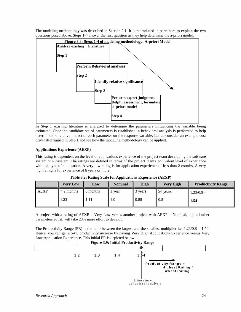
The modeling methodology was described in Section 2.1. It is reproduced in parts here to explain the twoquestions posed above. Steps 1-4 answer the first question as they help determine the a-priori model.
In Step 1 existing literature is analyzed to determine the parameters influencing the variable beingestimated. Once the candidate set of parameters is established; a behavioral analysis is performed to helpdetermine the relative impact of each parameter on the response variable. Let us consider an example costdriver determined in Step 1 and see how the modeling methodology can be applied.
Applications Experience (AEXP)
This rating is dependent on the level of applications experience of the project team developing the softwaresystem or subsystem. The ratings are defined in terms of the project team’s equivalent level of experiencewith this type of application. A very low rating is for application experience of less than 2 months. A veryhigh rating is for experience of 6 years or more.
Table 3.2: Rating Scale for Applications Experience (AEXP)
Very Low Low Nominal High Very High Productivity Range
AEXP � 2 months 6 months 1 year 3 years ≥6 years 1.23/0.8 =
1.23 1.11 1.0 0.88 0.8 1.54
A project with a rating of AEXP = Very Low versus another project with AEXP = Nominal, and all otherparameters equal, will take 23% more effort to develop.
The Productivity Range (PR) is the ratio between the largest and the smallest multiplier i.e. 1.23/0.8 = 1.54.Hence, you can get a 54% productivity increase by having Very High Applications Experience versus VeryLow Application Experience. This initial PR is depicted below.
Figure 3.9: Initial Productivity Range
Figure 3.8: Steps 1-4 of modeling methodology: A-priori Model
1 .54
L itera tu re ,b eh a v io ra l a n a ly sis
P ro d u ctiv ity R an g e =H ig h est R a tin g /L o w e st R a tin g
1 .2 1 .41 .3
Analyze existing literature
Step 1
Perform Behavioral analyses
Step 2
Identify relative significance
Step 3
Perform expert-judgmentDelphi assessment, formulate a-priori model
Step 4

Research Approach 25
After the initial PR is determined, a 2-Round Delphi analysis is carried out. This is currently being donewith nine experts (who are COCOMO II affiliates) and the results will be available shortly. A description ofhow it is being done is included here.
As described in chapter 2, the Delphi technique was originated at The Rand Corporation in 1948 and is aneffective way of getting group consensus. Based on literature and behavioral analysis an initial set of PRvalues was proposed for the model and the Delphi technique is being incorporated for further groupconsensus. On verbal suggestion from other experts who have used the Delphi technique, a 2-round Delphiprocess has been initiated. The steps being taken for the Delphi process are outlined below:
Round 1
1. Provide Participants with Round 1 Delphi Questionnaire with a proposed set of values for theProductivity Ranges
2. Receive responses
3. Ensure validity of responses by correspondence
Round 21. Provide participants with Round 2 Delphi Questionnaire -- based on analysis of Round 12. Repeat steps 2, 3, 4 (above)3. Converge to Final Delphi Results.
Subsections of the Round 1 Delphi Questionnaire are shown on the following page. Appendix B has thecomplete questionnaire that was provided to each of the participants.
Once the second round of the Delphi is completed, a new PR is defined which is the mean of the responsesreceived from the participants. The variance is computed from the different responses. This mean andvariance is then used as the prior nonsample information for the Bayesian analysis. As shown in the figurebelow, the mean of the responses is 1.42 and the variance is 0.09.
The Delphi results are used to determine the mean and variance of each of the 22 COCOMO II parameters.
A-Posteriori COCOMO II Post Architecture Model
Figure 3.10: A-Priori Productivity Range
1 .4 21 .5 4
L it e r a t u r e ,b e h a v io r a l a n a ly s i s
A - p r io r iE x p e r t s ’ D e lp h i
P ro d u c t iv i ty R a n g e =H ig h e s t R a t in g /L o w e s t R a t in g
1 .4 21 .5 4

Research Approach 26
Once, the a-priori model is determined, Steps 5 and 6 are carried out to develop the a-posteriori model.
The COCOMO II research effort started in 1994 and data is being collected since then. The data collectionactivity that has been continuously taking place is outlined below: 1. Define the data needed (to completely describe the Post Architecture Model)2. Collect data with a paper form or a computer software tool3.Affiliate Organizations provide majority of data
Historical - whole projectSite visits or phone interviews to record data
4.Enter the data into the repositoryData is labeled with generic idStored in locked roomLimited access by researchers
5.Do Data Consistency checking and conditioning
Step 5 of the data collection process is to ensure the validity of the data provided. For example, if AEXP =VL but PREC = VH then there are discrepancies in the data and the data reporter needs to be contacted formore information to resolve the inconsistencies.
The current database consists of 166 datapoints. The COCOMO II.1997 model was based on a dataset of 83datapoints. Statistical analyses exhibited high correlation among four of the 17 Effort Multipliers which ledto consolidating them into 15 Effort Multipliers [Devnani97]. The data was then divided into two subsets;one subset of 59 datapoints that was used for the regression analysis and the other subset of 24 projects thatwas used for cross validation. Multiple Regression Analyses on the first subset of 59 datapoints determinedthe coefficients for the 20 (now 15 Effort Multipliers + 5 Scale Factors) parameters. A 10% weightedaverage (using 10% of the data-driven values and 90% of the a-priori values) approach was used to adjustthe A-Priori expert-determined model parameters to obtain the calibrated “A-Posteriori Post ArchitectureModel” that reflected the characteristics of the actual 83 projects data. The 10% weighted averagetechnique was preferred over a pure least squares approach due to uncertainties that were apparent in thecontributed data.
Once, the A-Priori Post Architecture Model was calibrated; it was cross-validated using the second subsetof 24 datapoints. Prediction Accuracy was computed in terms of Proportional Error (PE) which had aNormal Distribution and the following accuracies (see next page) for Effort Prediction were observed (forexample, PRED(.30) = 64% means that 64% of the estimates were within 30% of the actuals).
Figure 3.11: Steps 5-6 of modeling methodology: A-posteriori Model
Gather project data
Step 5 Determine Bayesian A-Posteriori model
Step 6

Research Approach 27
Table 3.3: Prediction Accuaracies of COCOMO II.1997
In the above table, the column “Before Stratification by Organization” represents the Prediction Accuracyobtained by using the “A-Posteriori Post Architecture Model” on the 83 datapoints before any datastratification. On the other hand, the column “After Stratification by Organization” represents the PredictionAccuracy obtained by using the “A-Posteriori Post Architecture Model” on the 83 datapoints afterstratifying the data by organization* and computing a new multiplicative constant for each of theorganizations. It is clear from the above table that simple local calibration helps in improving the predictionaccuracy of the model.
The successive versions of the COCOMOII model are summarized below.
Successive versions of COCOMO II• The 1997 version
Multivariate Linear Regression with 10% weighted average of expert-determined and datadetermined
• The 1998 versionBayesian Regression AnalysisWeighted averageSeparate weights for each parameter based on significanceModel more Data-Determined
• The 19??/20?? Version
Figure 3.12: Successive version of COCOMO II100%
Data-Determined
* Stratification “by Organization” does not mean “by Application Type”. In the COCOMO II database, wehave actual project data from seven relatively homogeneous sources and the data was stratified into sevensets based on the source of the data.
Prediction Before Stratification by Organization After Stratification by OrganizationPRED(.20) 46% 49%PRED(.25) 49% 55%PRED(.30) 52% 64%
Evolving Model Values
Number of projects used in calibration
100% ExpertDriven
100% DataDriven
100
50
100
10
500 1000
Linear Regression - COCOMO II.1997 version
Our aim
Bayesian Analysis
Research Approach 28
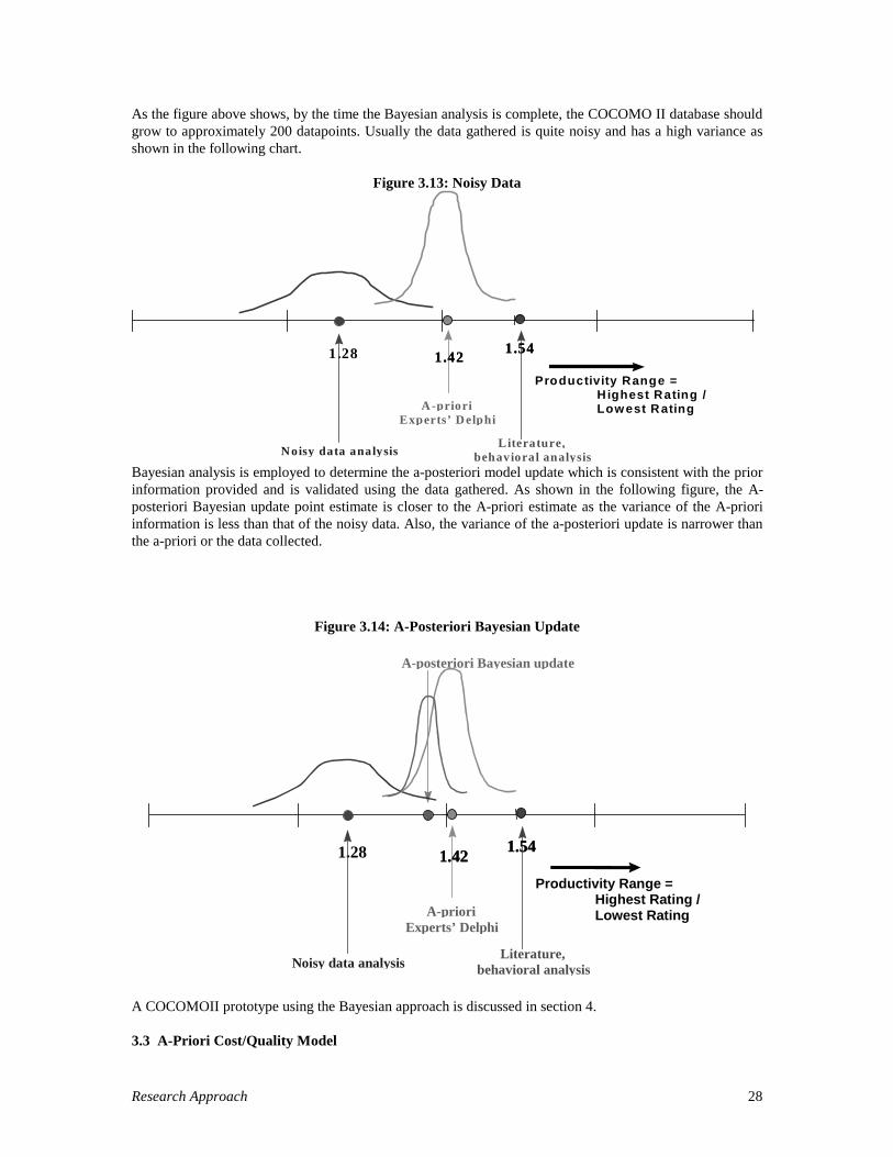
As the figure above shows, by the time the Bayesian analysis is complete, the COCOMO II database shouldgrow to approximately 200 datapoints. Usually the data gathered is quite noisy and has a high variance asshown in the following chart.
Figure 3.13: Noisy Data
1.421.541.28
Literature,behavioral analysis
A -prioriExperts’ Delphi
N oisy data analysis
Productivity Range =Highest Rating /Low est R ating
1.421.54
Bayesian analysis is employed to determine the a-posteriori model update which is consistent with the priorinformation provided and is validated using the data gathered. As shown in the following figure, the A-posteriori Bayesian update point estimate is closer to the A-priori estimate as the variance of the A-prioriinformation is less than that of the noisy data. Also, the variance of the a-posteriori update is narrower thanthe a-priori or the data collected.
Figure 3.14: A-Posteriori Bayesian Update
1.421.541.28
Literature,behavioral analysis
A-prioriExperts’ Delphi
Noisy data analysis
A-posteriori Bayesian update
Productivity Range =Highest Rating /Lowest Rating
1.421.54
A COCOMOII prototype using the Bayesian approach is discussed in section 4.
3.3 A-Priori Cost/Quality Model

Research Approach 29
The model depicted in Figure 3.15 shows that defects conceptually flow into a holding tank through variousdefect-source pipes & are drained off through various defect-elimination pipes. The defect source pipes aremodeled as the “Software Defect Introduction Model” and the defect elimination pipes are modeled as the“Software Defect Removal Model”.
Section 3.3.1 describes the Defect Introduction model which is published in [Chulani97B]. The formulationof the defect removal model is ongoing and is described in Chapter 4: Status and Plans.
3.3.1 Defect Introduction ModelAs depicted above, the Software Cost/Quality model is composed of the (i) Defect Introduction model andthe (ii) Defect Removal model. The focus of this section is to show how the methodology described in theprevious section was incorporated to develop the a-priori cost/quality model.
Defects can be introduced in several activities of the software development life cycle and are classifiedbased on their origin. The four types of defect artifacts based on this classification for the focus of thisresearch are Requirements Defects (e.g. leaving out a required Cancel option in an Input screen), DesignDefects (e.g. error in the algorithm) and Coding Defects (e.g. looping 9 instead of 10 times). Capers Jones[16] in the glossary of his book under “Defect Origins” also has a category called “bad fixes”. For themodel discussed in this paper, “bad fixes” are accounted for by the varying ratings of certain DIR drivers(for example, Analyst Capability).
Research results reported in [Jones78, Thayer78; Boehm80] show the overall Defect Introduction Rate(DIR) as 45 defects/KDSI of which 5/KDSI are Requirements defects, 25/KDSI are Design defects and15/KDSI are Coding defects. For the Defect Introduction model described in this paper these rates will beused as baseline DIRs. Hence, the baseline Defect Introduction Rates (DIRBaseline) for this model are:
Table 3.4: Baseline Defect Introduction Rates of the late 1970sType of Artifact DIRBaseline
Requirements Defects 5/KDSIDesign Defects 25/KDSI
Figure 3.15: Software Defect Introduction and Removal Model
• • •
Documentation Defects
Residual
Software
Defects
Code Defects
Requirements Defects
Design Defects
Defect Introduction pipes
Defect Removal pipes

Research Approach 30
Coding Defects 15/KDSI
Using the above baseline rates, the Nominal2 Defect Introduction (DINom) for each type of defect artifact, j,can be formulated as
DINom j = DIRBaseline j X (Size)B Eq 3.12
And for now, B (which is equivalent to the Scale Factors in COCOMO II) is set to 1. Further investigationof this parameter is required but can be carried out when enough project data is available. It is unclear ifDefect Introduction Rates will exhibit economies or diseconomies of scale as indicated in [Banker94] and[Gulledge93]. The question is if Size doubles, then will the Defect Introduction Rate increase by more thantwice the original rate? This would indicate diseconomies of scale implying B > 1. Or will DefectIntroduction Rate increase by a factor less than twice the original rate, indicating economies of scale,giving B < 1?
Equation 3.12 doesn’t capture the effects of hardware constraints, personnel quality and experience, use ofmodern tools and techniques, and other significant parameters. It models Defect Introduction as a functionof the baseline DIR and Size. This DIR is good for an order-of-magnitude estimate, but additional factorsare necessary for better estimates of individual projects. Equation 4 is similar to the BASIC COCOMO ’81model equation. To increase the accuracy of the Defect Introduction model, the author used a set of 22significant DIR drivers which was the result of step 1 of the modeling methodology. Steps 2-4 are describedfurther in the following section.
Equation 3.13 formulates the Estimated DI (DIEst) as a function of the baseline DIR, Size and the 22 DIR-drivers. The DIR-drivers (discussed later) are aggregated as a product into a Quality Adjustment Factor forDefect Introduction (QAFDI). For each type of artifact, j,
DIEst j = Aj X DINom j X QAFDI; j Eq 3.13
where :Aj = Calibration Constant for the jth artifactQAFDI; j = Quality Adjustment Factor for each type of artifact (Requirements, Design, Coding)
For each type of artifact, j,
QAFDI; j
DIR - driverij
i 1
22=
=
∏ Eq 3.14
Summarizing, we haveRequirements Defects Introduced (DIEst ; req )
= Areq X DINom; req X QAFDI; req
Design Defects Introduced (DIEst; des )
= Areq X DINom; des X QAFDI; des
Coding Defects Introduced (DIEst cod )
= Acod X DINom; cod X QAFDI; cod
Total Defects Introduced= Σ [Aj X (Size)B X QAFj ] Eq 3.15
2 The “nominal” level of defects is without the effect of the 22 project-specific DIR drivers.

Research Approach 31
The model formulated in Equation 3.15 is analogous to the Intermediate COCOMO ’81 model and theCOCOMO II Post Architecture model
Example of the application of the Defect Introduction ModelThe model described above can be illustrated using a simple example. Lets say, the Size of the softwareproduct is 4KSLOC. The nominal level of Defects Introduced for each type of artifact can then bycomputed as shown
DINom; req = DIRBaseline; req X (Size)B = 5 X 4 = 20DINom; des = DIRBaseline; des X (Size)B = 25 X 4 = 100DINom; cod = DIRBaseline; cod X (Size)B = 15 X 4 = 60
Hence,Nominal Defects Introduced (DINom ) = 180
Now, suppose the same product is developed by analysts rated at the 90th percentile and the other DIRdrivers remain unchanged. From the description of the COCOMO II parameters [19], the Analyst Capability(ACAP) rating is set to Very High. The corresponding rating (discussed in Section 4) for ACAPreq=VH is0.75, ACAPdes = VH is 0.83 and ACAPcod = VH is 0.90 resulting in QAFDI; req = 0.75, QAFDI; des = 0.83 andQAFDI; cod = 0.90 with every other parameter set at Nominal. Lets say, calibration3 results yield Areq = 1.5,Ades = 0.75 and Acod = 1.0 for the four multiplicative constants. The level of Defect Introduction will be asfollows
DIEst; req = 1.5 X 20 X 0.75 = 22DIEst; des = 0.75 X 100 X 0.83 = 62DIEst; cod = 1.0 X 60 X 0.90 = 54
Hence,Total Defects Introduced = 138
The above example clearly shows the reduction in the number of defects introduced by having goodanalysts on the development team.
Behavioral Analyses and Delphi ProcessA thorough behavioral analyses for each DIR driver was done (Step 2 of Modeling Methodology). Anexample is provided in Table 4.
For the empirical formulation of the Defect Introduction Model, as with COCOMO II, it was essential toassign numerical values to each of the ratings of the DIR drivers. Based on expert-judgment an initial set ofvalues was proposed for the model (Step 3 of Modeling Methodology). The DIR drivers range from VL(very low) to XH (extra high) and depending on their corresponding values either increase or decrease thelevel of defect introduction as compared to the nominal level of defect introduction. If the DIR driver > 1then it has a detrimental effect on the DIR and overall software quality; and if the DIR driver < 1 then itreduces the DIR increasing the quality of the software being developed. This is analogous to the effect theCOCOMO II Multiplicative Cost Drivers have on Effort.
A 2-round Delphi [12] was incorporated for further group consensus (Step 4 of Modeling Methodology).Readers not familiar with the above techniques can refer to Chapter 22 of [3] for an overview of commonmethods used for software estimation.
The Delphi process was formulated using the “Quality Range due to Defect Intorduction” for each DIRdriver; defined as the ratio between the largest DIR driver and the smallest DIR driver. The nineparticipants selected for the Delphi process were representatives of Commercial, Aerospace, Government
3 The calibration process is still in progress and hence the values of Areq, Ades, Acod have been assumed.

Research Approach 32
and FFRDC and Consortia organizations. Each of the participants had notable expertise in the area ofSoftware Metrics and Quality Management and hence contributed significantly to the initial version of themodel.
The steps that the author took for the entire Delphi process are outlined below.
Round 1 - Steps1 Provided Participants with Round 1 Delphi Questionnaire with a proposed set of values for the QualityRanges. This set was proposed based on experience.2 Received nine completed Round 1 Delphi Questionnaires.3 Ensured validity of responses by correspondence with the participants.4 Did simple analysis based on ranges and medians of the responses.
Round 2 - Steps1 Provided participants with Round 2 Delphi Questionnaire -- based on analysis of Round 1.2 Repeated steps 2, 3, 4 (above)
3 Converged to Final Delphi Results which resulted in the definition of the initial model
An Example Defect Introduction Rate DriverAn example of how the Delphi process was carried out is shown using the Analyst Capability DIR driver.Analysts are personnel that work on requirements, high level design and detailed design. The majorattributes that should be considered in this rating are Analysis and Design ability, efficiency andthoroughness, and the ability to communicate and cooperate effectively. Analysts that fall in the 15thpercentile are rated very low and those that fall in the 95th percentile are rated very high as shown in Table3.5.
Table 3.6 explainsthe impact ACAPhas on the DefectIntroduction Ratefor the two extreme values i.e. VH and VL.
If ACAP = VH then the Number of Defects Introduced is lower as compared to ACAP = VL. Based onexpert judgment a value of 0.75 is assigned to ACAPreq = VH. This means that the Defect Introduction Rateof Requirements Defects is reduced by 75% if the rating of Analyst Capability is VH. Similar explanationcan be given for the other ratings. Note again, that the Nominal rating is always 1.0.
Table 3.5: Analyst Capability Ratings
Very Low Low Nominal High Very High
ACAP 15thpercentile
35thpercentile
55thpercentile
75thpercentile
90thpercentile

Research Approach 33
As explained above, in Step 1 of Round 1, the author provided the nine participants with the Initial QualityRange due to Defect Introduction. Hence, as shown in the above table, Initial Quality Range due to DefectIntroduction for the Requirements activity is 1.33/0.75 = 1.77. After about 3 weeks, the author received theresponses from Round 1. After validating the responses with direct correspondence with some of theparticipants; the author did a simple analysis and derived the range and median of the responses. The resultsof this analysis, shown in the table as Range - Round1 and Median - Round 1, were provided to theparticipants along with their Round 1 response. This was the first step of Round 2. Again, after a turnaround of about 2 weeks, the Round 2 results came in and a similar analysis (as in Round 1) was done. Themedian of the Round 2 responses resulted in the Final Quality Range due to Defect Introduction. It wasobserved that the range in Round 2 was typically narrower than the range in Round 1.
New DIR drivers for the several intermediate levels were computed using the Final Quality Range due toDefect Introduction. For example, the Final Quality Range for Requirements Defects due to ACAP is 1.77.The Very Low and Very High ratings associated with ACAP for Requirements Defects were computedusing geometric interpolation as shown below
DIR Driver VeryLow FinalQualityRangeduetoDefectIntroduction− =( ) = 177. = 1.33
and
DIR-Driver(VeryHigh) = ( FinalQualityRangeduetoDefectIntroduction )-1 =( 177. )-1= 0.75
Eq. 3.16
Table 3.6: Analyst Capability (ACAP) Differences in Defect IntroductionACAP level Requirements Design CodeVH Fewer Requirements
understanding defectsFewer RequirementsCompleteness, consistencydefects
0.75
Fewer Requirementstraceability defectsFewer DesignCompleteness, consistencydefectsFewer defects introduced infixing defects
0.83
Fewer Coding defectsdue to requirements,design shortfalls-missing guidelines-ambiguities
0.90
Nominal Nominal level of defect introduction 1.0VL More Requirements
understanding defectsMore RequirementsCompleteness, consistencydefects
1.33
More Requirementstraceability defectsMore DesignCompleteness, consistencydefectsMore defects introduced infixing defects
1.20
More Coding defects dueto requirements, designshortfalls-missing guidelines-ambiguities
1.11
Initial Quality Range 1.77 1.45 1.23Range - Round 1 1.4-2 1.3-1.8 1-1.4Median - Round 1 1.92 1.48 1.23Range - Round 2 1.7-2 1.4-1.69 1.2-1.41Final Quality Range 1.77 1.45 1.23

Research Approach 34
Example : Consider a software project which has 100 Requirements Defects, and has analysts of nominallevel of capability working on it. Suppose, now the team of analysts is replaced by very-high rated analysts.Assume also that all other parameters remain unchanged.
Using table 3.7, the number of Requirements Defects will be reduced to 75 (100 X 0.75). The reasons for
the decrease in the number of defects introduced in the Requirements activity are presented in table 3.6.Thus the 25% decrease in Requirements Defects is due to the very-high level of capability of the analystscausing fewer Requirements understanding and Requirements Completeness, Consistency defects ascompared to nominal level.
The values assigned to ACAP for each type of artifact are graphically represented in Figure 3.16 andsummarized in Table 5. From the figure, it can be seen that ACAP = VH results in ACAPreq = 0.75.Similarly, the other ratings are also represented graphically.
A detailed description of each of the other 21 DIR drivers and its impact on defect introduction for eachtype of defect artifact can be found in appendix C.
Software Quality Range due to Defect Introduction‘Quality Range due to Defect Introduction’ is the ratio between the largest DIR driver and the DIR driver. Itis an indicator of the relative ability of the attribute to affect software quality.
Figure 3.17 provides a graphical view of the relative Quality Ranges due to Defect Introduction ofRequirements Defects provided by the 22 Defect Driver Attributes. It shows each factor’s Quality Rangedue to Defect Introduction. If all other Defect Driver Attributes are held constant, a Very Low (VL) ratingfor Disciplined Methods (DISC)will result in a software project with 2.5 times the number of residualRequirements Defects as compared to a Very High (VH) rating.
Figure 3.16: Analyst Capability (ACAP) for each Type of Artifact
0.6
0.7
0.8
0.9
1
1.1
1.2
1.3
1.4
Requirements Design Coding
Very High
High
Nominal
Low
Very Low
Table 3.7: Analyst Capability (ACAP) DIR DriverACAP level Type of Artifact
Requirements Design Coding
Very High 0.75 0.83 0.90High 0.87 0.91 0.95Nominal 1.0 1.0 1.0Low 1.15 1.10 1.05Very Low 1.33 1.20 1.11

Research Approach 35
3.3.2 Data Collection
Severity of DefectsFor the purpose of the data collection activity and for a stronger model, the defects were categorized basedon severity. Parts of the data collection form are reproduced on the following page.
Figure 3.17: Software Quality Range due to Requirements Defects Introduction
1.00 1.20 1.40 1.60 1.80 2.00 2.20 2.40 2.60
DISC
RELY
PREC
PMAT
TEAM
ACAP
CPLX
RESL
AEXP
PCON
SITE
SCED
DOCU
PVOL
PEXP
TOOL
DATA
LTEX
RUSE
TIME
STOR
PCAP

Research Approach 36
After the data is collected, the ‘low’ and ‘none’ severity defects are ignored and analysis is done only on thesum of ‘critical’, ‘high’ and ‘medium’ severity defects. Hence, using the Cost/Quality model described thenumber of critical+high+medium defects is estimated. Once enough data is collected, the ratio of number oflow+none defects / number of critical+high+medium defects can be estimated and this ratio can then beused to determine the total number of defects in a product rather than just the number ofcritical+high+medium defects.
4 Adapted from IEEE Std 1044.1-1995
2.18 Severity of Defects. Categorize the several defects based on their severity using the followingclassification4 information:
• Critical
Causes a system crash or unrecoverable data loss or jeopardizes personnel.
The product is unusable (and in mission/safety software would prevent the completion of themission).
• High
Causes impairment of critical system functions and no workaround solution exists.
Some aspects of the product do not work ( and the defect adversely affects successful completion ofmission in mission/safety software), but some attributes do work in its current situation.
• Medium
Causes impairment of critical system function, though a workaround solution does exist.
The product can be used, but a workaround (from a customer's preferred method of operation) mustbe used to achieve some capabilities. The presence of medium priority defects usually degrades thework.
• Low
Causes a low level of inconvenience or annoyance.
The product meets its requirements and can be used with just a little inconvenience. Typos indisplays such as spelling, punctuation, and grammar which generally do not cause operationalproblems are usually categorized as low severity.
• None
Concerns a duplicate or completely trivial problem, such as a minor typo in supportingdocumentation.
Critical and High severity defects result in an approved change request or failure report.

Research Approach 37
Types of Defect Artifacts
Defects can be introduced in several activities of the software development life cycle and are classifiedbased on their origin. The four types of defect artifacts based on this classification for the focus of thisresearch are Requirements Defects (e.g. leaving out a required Cancel option in an Input screen), DesignDefects (e.g. error in the algorithm) and Coding Defects (e.g. looping 9 instead of 10 times). Capers Jones[16] in the glossary of his book under “Defect Origins” also has a category called “bad fixes”. For themodel discussed in this paper, “bad fixes” are accounted for by the varying ratings of certain DIR drivers(for example, Analyst Capability).
A portion of the data collection form that captures this information is reproduced here
2.19 Defect Introduction by Artifact. The software development process can be viewed as introducing a certain number ofdefects into each software product artifact. Enter the number of defects introduced in the several artifacts involved in thesoftware development process.
Artifact Requirements Design Coding Documentation
No. of defects introduced
A Requirements Defect is a defect introduced in the Requirements Activity and a Design Defect is a defect introduced in theDesign activity and so on and so forth.
2.19.1 Requirements Defects
Severity Urgent High Medium Low None
No. of Requirements Defects
2.19.2 Design Defects
Severity Urgent High Medium Low None
No. of Design Defects
2.19.3 Coding Defects
Severity Urgent High Medium Low None
No. of Coding Defects

Research Approach 38
Overall Data Reporting Scheme
Table 3.8: Data Reporting Scheme
Activity →Discovered + Unresolved / Resolved in Activity/Cost To Resolve by Activity
Type of Artifact ↓Reqts Design Code
& UnitTest
SWInteg.andTest
SWAcceptanceTest
SystemImpleme-ntationand Test
Post-Oper-ational
Other
Requirements 50/30/.2
20+20/20/.5
10+20/15/1.0
2+15/10/1.5
1+7/6/4 ...
Design 55/25/1.0
15+30/25/2.5
... ... ...
Code ... ... ... ...
Table 3.8 gives the overall picture of the data collected to model the Cost/Quality model. Since, only‘critical’, ‘high’ and ‘medium’ severity defects are accounted for the table is kept simple by ignoring theseverity.
To understand the table, lets consider the first cell marked 50/30/.2 - 50 Requirements Defects wereintroduced in the Requirements activity; of which 30 were resolved in the Requirements activity; and theaverage cost to resolve each Requirements defect is .2 units (for example, 0.2 person hours). Now, letsconsider the second cell marked 20+20/20/.5 - 20 new Requirements defects were discovered in the Designactivity and 20 (50-30) were carried over from the Requirements activity; of which 20 were resolved in theDesign activity; and the average cost to resolve each Requirements defect is .5 units (for example, 0.2person hours). Note, that that cost to resolve a Requirements defect increases as the defect propagatesthrough the several activities of the development process. This is consistent with published results from[Boehm, etc.].
The current status of the cost/quality model is summarized in chapter 4 of this proposal.
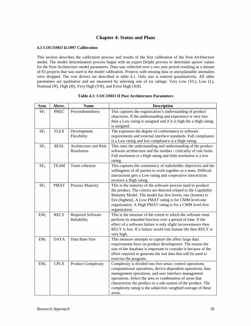
Research Approach 39
Chapter 4: Status and Plans
4.1 COCOMO II.1997 Calibration
This section describes the calibration process and results of the first calibration of the Post-Architecturemodel. The model determination process began with an expert Delphi process to determine apriori valuesfor the Post-Architecture model parameters. Data was collected over a two year period resulting in a datasetof 83 projects that was used in the model calibration. Projects with missing data or unexplainable anomalieswere dropped. The cost drivers are described in table 4.1. Only size is entered quantitatively. All otherparameters are qualitative and are measured by selecting one of six ratings: Very Low (VL), Low (L),Nominal (N), High (H), Very High (VH), and Extra High (XH).
Table 4.1: COCOMO II Post Architecture Parameters
Sym. Abrev. Name DescriptionSF1 PREC Precendentedness This captures the organization’s understanding of product
objectives. If the understanding and experience is very lowthen a Low rating is assigned and if it is high the a High ratingis assigned.
SF2 FLEX DevelopmentFlexibility
The expresses the degree of conformance to softwarerequirements and external interface standards. Full complianceis a Low rating and low compliance is a High rating.
SF3 RESL Architecture and RiskResolution
This rates the understanding and understanding of the productsoftware architecture and the number / criticality of risk items.Full resolution is a High rating and little resolution is a lowrating.
SF4 TEAM Team cohesion This captures the consistency of stakeholder objectives and thewillingness of all parties to work together as a team. Difficultinteractions gets a Low rating and cooperative interactionsreceives a High rating.
SF5 PMAT Process Maturity This is the maturity of the software process used to producethe product. The criteria are directed related to the CapabilityMaturity Model. The model has five levels, one (lowest) tofive (highest). A Low PMAT rating is for CMM level-oneorganization. A High PMAT rating is for a CMM level-fiveorganization.
EM1 RELY Required SoftwareReliability
This is the measure of the extent to which the software mustperform its intended function over a period of time. If theeffect of a software failure is only slight inconvenience thenRELY is low. If a failure would risk human life then RELY isvery high.
EM2 DATA Data Base Size This measure attempts to capture the affect large datarequirements have on product development. The reason thesize of the database is important to consider it because of theeffort required to generate the test data that will be used toexercise the program.
EM3 CPLX Product Complexity Complexity is divided into five areas: control operations,computational operations, device-dependent operations, datamanagement operations, and user interface managementoperations. Select the area or combination of areas thatcharacterize the product or a sub-system of the product. Thecomplexity rating is the subjective weighted average of theseareas.

Status and Plans 40
Sym. Abrev. Name DescriptionEM4 RUSE Required Reusability This cost driver accounts for the additional effort needed to
construct components intended for reuse on the current orfuture projects. This effort is consumed with creating moregeneric design of software, more elaborate documentation, andmore extensive testing to ensure components are ready for usein other applications.
EM5 DOCU DocumentationMatch to Life-cycleNeeds
The rating scale for the DOCU cost driver is evaluated interms of the suitability of the project’s documentation to itslife-cycle needs. The rating scale goes from Very Low (manylife-cycle needs uncovered) to Very High (very excessive forlife-cycle needs).
EM6 TIME Time Constraint Execution Time Constraint. This is a measure of the executiontime constraint imposed upon a software system. The ratingranges from nominal (less than 50%) of the execution timeresource used, to extra high (95%) of the execution timeresource is consumed.
EM7 STOR Storage Constraint Main Storage Constraint. This rating represents the degree ofmain storage constraint imposed on a software system orsubsystem. The rating ranges from nominal (less that 50%) toextra high (95%).
EM8 PVOL Platform Volatility “Platform” is used here to mean the complex of hardware andsoftware (OS, DBMS, etc.) the software product calls on toperform its tasks. The platform includes any compilers orassemblers supporting the development of the softwaresystem. This rating ranges from low, where there is a majorchange every 12 months, to very high, where there is a majorchange every two weeks.
EM9 ACAP Analyst Capability Analyst Capability. Analysts are personnel that work onrequirements, high level design and detailed design. The majorattributes that should be considered in this rating are Analysisand Design ability, efficiency and thoroughness, and theability to communicate and cooperate. The rating should notconsider the level of experience of the analyst; that is ratedwith AEXP. Analysts that fall in the 15th percentile are ratedvery low and those that fall in the 95th percentile are rated asvery high.
EM10 PCAP ProgrammerCapability
Programmer Capability. Evaluation should be based on thecapability of the programmers as a team rather than asindividuals. Major factors which should be considered in therating are ability, efficiency and thoroughness, and the abilityto communicate and cooperate. The experience of theprogrammer should not be considered here; it is rated withAEXP. A very low rated programmer team is in the 15thpercentile and a very high rated programmer team is in the95th percentile.
EM11 AEXP ApplicationsExperience
This rating is dependent on the level of applicationsexperience of the project team developing the software systemor subsystem. The ratings are defined in terms of the projectteam’s equivalent level of experience with this type ofapplication. A very low rating is for application experience ofless than 2 months. A very high rating is for experience of 6years or more.

Status and Plans 41
Sym. Abrev. Name DescriptionEM12 PEXP Platform Experience The Post-Architecture model broadens the productivity
influence of PEXP, recognizing the importance ofunderstanding the use of more powerful platforms, includingmore graphic user interface, database, networking, anddistributed middleware capabilities.
E13 LTEX Language and ToolExperience
This is a measure of the level of programming language andsoftware tool experience of the project team developing thesoftware system or subsystem. A low rating given forexperience of less than 2 months. A very high rating is givenfor experience of 6 or more years.
EM14 PCON Personnel Continuity The rating scale for PCON is in terms of the project’s annualpersonnel turnover: from 3%, very high, to 48%, very low.
EM15 TOOL Use of SoftwareTools
The tool rating ranges from simple edit and code, very low, tointegrated lifecycle management tools, very high.
EM16 SITE Multi-SiteDevelopment
Determining this rating involves the assessment and averagingof two factors: site collocation (from fully collocated tointernational distribution) and communication support (fromsurface mail and some phone access to full interactivemultimedia).
EM17 SCED RequiredDevelopmentSchedule
This rating measures the schedule constraint imposed on theproject team developing the software. The ratings are definedin terms of the percentage of schedule stretch-out oracceleration with respect to a nominal schedule for a projectrequiring a given amount of effort. Accelerated schedules tendto produce more effort in the later phases of developmentbecause more issues are left to be determined due to lack oftime to resolve them earlier. A schedule compress of 74% israted very low. A stretch-out of a schedule produces moreeffort in the earlier phases of development where there is moretime for thorough planning, specification and validation. Astretch-out of 160% is rated very high
The cost drivers had apriori values assigned to each of ratings. Not all six rating levels were valid for allcost drivers. The values are given in table 4.2 below.
Table 4.2: A-priori Values
Driver Symbol VL L N H VH XHPREC SF1 0.05 0.04 0.03 0.02 0.01 0.0FLEX SF2 0.05 0.04 0.03 0.02 0.01 0.0RESL SF3 0.05 0.04 0.03 0.02 0.01 0.0TEAM SF4 0.05 0.04 0.03 0.02 0.01 0.0PMAT SF5 0.05 0.04 0.03 0.02 0.01 0.0RELY EM1 0.75 0.88 1.00 1.15 1.40DATA EM2 0.94 1.00 1.08 1.16CPLX EM3 0.75 0.88 1.00 1.15 1.30 1.65RUSE EM4 0.89 1.00 1.16 1.34 1.56DOCU EM5 0.85 0.93 1.00 1.08 1.17TIME EM6 1.00 1.11 1.30 1.66STOR EM7 1.00 1.06 1.21 1.56PVOL EM8 0.87 1.00 1.15 1.30ACAP EM9 1.5 1.22 1.00 0.83 0.67

Status and Plans 42
PCAP EM10 1.37 1.16 1.00 0.87 0.74PCON EM11 1.26 1.11 1.00 0.91 0.83AEXP EM12 1.23 1.10 1.00 0.88 0.80PEXP EM13 1.26 1.12 1.00 0.88 0.80LTEX EM14 1.24 1.11 1.00 0.9 0.82TOOL EM15 1.20 1.10 1.00 0.88 0.75SITE EM16 1.24 1.10 1.00 0.92 0.85 0.79SCED EM17 1.23 1.08 1.00 1.04 1.10
Model parameters that exhibited high correlation were consolidated i.e. TIME and STOR were combinedinto RCON (Resource Constraints) since the correlation between them was XX. ACAP and PCAP werecombined into PERS (Personnel factors) since the correlation between them was XX. Multiple regressionanalysis was used to produce coefficients for the transformed log-log model. The resulting coefficients arerepresented in table 4.3.
Table 4.3: Estimated Coefficients from Multivariate Linear RegressionCoefficient Estimate Coefficient Estimate
B0 for A 0.70188 B11 for EM1 (PVOL) 0.85830B1 for SF1 (PREC) -0.90196 B12 for EM1 (AEXP) 0.56053B2 for SF2 (FLEX) 3.14218 B13 for EM1 (PEXP) 0.69690B3 for SF3 (RESL) -0.55861 B14 for EM1 (LTEX) -0.04214B4 for SF4 (TEAM) 0.86614 B15 for EM1 (PCON) 0.30826B5 for SF5 (PMAT) 0.08844 B16 for EM1 (TOOL) 2.49512B6 for EM1 (RELY) 0.79881 B17 for EM1 (SITE) 1.39701B7 for EM1 (DATA) 2.52797 B18 for EM1 (SCED) 2.84075B8 for EM1 (RUSE) -0.44410 B19 for EM1 (PERS) 0.98747B9 for EM1 (DOCU) -1.32819 B20 for EM1 (RCON) 1.36588B10 for EM1 (CPLX) 1.13191
The multivariate linear regression yields negative coefficients for a few of the parameters. For example, Bfor RUSE = -0.44. These negative coefficient estimates do not support the ratings for which the data wasgathered. To see the effect of a negative coefficient, table 4.4 gives the ratings, apriori values, and fullydata-determined values for RUSE. Based on the definition of the Required Reusability cost driver, RUSE,the apriori model values indicate that as the rating increases from Low (L) to Extra High (XH), the amountof required effort will also increase. This rationale is consistent with the results of 12 studies of the relativecost of writing for reuse compiled in [Poulin97]. The adjusted values determined from the data sampleindicate that as more software is built for wider ranging reuse less effort is required. As shown in 4.2 this isinconsistent with experience.
Table 4.4: Required Reusability (RUSE)RUSE L N H VH XH
Definition None Across project Acrossprogram
Across productline
Across multipleproduct lines
Apriori Values 0.89 1.00 1.16 1.34 1.56Data-
DeterminedValues
1.05 1.00 0.94 0.88 0.82
A possible explanation for the phenomenon is the frequency distribution of the data used to calibrate RUSE.There were a lot of responses that were “I don’t know” or “It does not apply.” These are essentially treatedas Nominal in the model. Hence, the data does not exhibit enough dispersion along the entire range ofpossible values for RUSE. Note than a little over 50 of the 83 datapoints have RUSE = Nominal as shownin figure 4.1.

Status and Plans 43
Due to the noisy data collected, for the calibration of the COCOMO II.1997 model only 10% of the effectof the estimated coefficients were applied to the apriori model parameters. The 10% weighting factor wasselected after comparison runs using 0% and 25% weighing factors were found to produce less accurateresults that the 10% factors. This moved the model parameters in the direction suggested by the regressioncoefficients but retained the rationale contained within the apriori values.
An example of the 10% application is given in figure 4.2. The distance between the apriori values and thedata-determined coefficient values is shown for each rating. 10% of the distance between from apriori and90% of the distance from data-determined is taken as the 1997 calibrated value for RUSE.
Figure 4.2: RUSE rating scale
0.80
0.90
1.00
1.10
1.20
1.30
1.40
1.50
1.60
L N H VH XH
Apriori
10% Regression
100% Regression
Using 10% of the data-driven and 90% of the apriori values, table 4.5 shows the COCOMO II.1997calibrated values. The constant, A, evaluates to 2.45.
Figure 4.1: Distribution of RUSE
XH VH HNL
50
40
30
20
10
0
RUS E
Freq
uenc
y

Status and Plans 44
Table 4.5: COCOMO II.1997 ValuesDriver Symbol VL L N H VH XHPREC SF1 0.0405 0.0324 0.0243 0.0162 0.0081 0.00FLEX SF2 0.0607 0.0486 0.0364 0.0243 0.0121 0.00RESL SF3 0.0422 0.0338 0.0253 0.0169 0.0084 0.00TEAM SF4 0.0494 0.0395 0.0297 0.0198 0.0099 0.00PMAT SF5 0.0454 0.0364 0.0273 0.0182 0.0091 0.00RELY EM1 0.75 0.88 1.00 1.15 1.39DATA EM2 0.93 1.00 1.09 1.19CPLX EM3 0.75 0.88 1.00 1.15 1.30 1.66RUSE EM4 0.91 1.00 1.14 1.29 1.49DOCU EM5 0.89 0.95 1.00 1.06 1.13TIME EM6 1.00 1.11 1.31 1.67STOR EM7 1.00 1.06 1.21 1.57PVOL EM8 0.87 1.00 1.15 1.30ACAP EM9 1.50 1.22 1.00 0.83 0.67PCAP EM10 1.37 1.16 1.00 0.87 0.74PCON EM11 1.24 1.10 1.00 0.92 0.84AEXP EM12 1.22 1.10 1.00 0.89 0.81PEXP EM13 1.25 1.12 1.00 0.88 0.81LTEX EM14 1.22 1.10 1.00 0.91 0.84TOOL EM15 1.24 1.12 1.00 0.86 0.72SITE EM16 1.25 1.10 1.00 0.92 0.84 0.78SCED EM17 1.29 1.10 1.00 1.00 1.00
The resulting a-posteriori model produces estimates within 30% of the actuals 52% of the time for effort.
Table 4.6: Prediction Accuracy of COCOMO II.1997PRED(.20) 46%PRED(.25) 49%PRED(.30) 52%
The flaw of COCOMO II.1997 is the uniform weighted average of 10% assigned to every parameter. Notall calibrated variables behave like RUSE. For example, B for PERS = 0.99; and the data collected on thisfactor is not as noisy as that collected for RUSE. The factor PERS is well-understood and on this parameterdata has been collected since many years. It is not as new a concept as RUSE. Hence, more weight shouldbe given to the data-determined value i.e. depending on the variance of the collected data and the aprioriconfidence for each parameter, a weighted average should be appropriately selected. This is the approachtaken by the Bayesian technique. Figure 4.3 illustrates the 10% weighted average approach and theBayesian approach. The assumption being made for this proposal is that the prediction accuracy ofCOCOMO II will improve using Bayesian techniques. The purpose of my research is to test this hypothesis.
Figure 4.3: COCOMO II Calibration Approaches
10% weighted-average update
1.541.28
A-prioriExpert-determined
Noisy data analysis
Productivity Range =Highest Rating /Lowest Rating
1.54 1.421.541.28
Literature,behavioral analysis
A-prioriExperts’ Delphi
Noisy data analysis
A-posteriori Bayesian update
Productivity Range =Highest Rating /Lowest Rating
1.421.54

Status and Plans 45
This can be done by splitting the dataset into two sets such that one set is used for calibration purposes (the“calibration” set) and the other randomly selected set of datapoints is used as a “validation” set. If theaccuracy using the validation set is higher using the Bayesian technique versus using the standard OLSapproach then the answer to the research question is positive.
4.2 COCOMOII Bayesian Prototype
In the previous section, the Bayesian Approach for COCOMO II was described. The Delphi process thatwas illustrated will be used to determine the a-priori information. The data collected (166 datapoints as ofnow) will be used as sampling data and the regression coefficients derived using multivariate linearregression will be adjusted based on the variance of the data and the prior information to yield the posteriorregression coefficients.
Since, the Delphi process is not complete, the prior information that was used for the 1997 calibration hasbeen used. The variance associated with each parameter has been assumed.
A simplified cost model can be denoted as
Effort A Size EMBi
i
= ∏( ) Eq. 4.1
where B = 1.01 + 0.01 (PREC+FLEX+TEAM+RESL+PMAT)and EM = Effort Multiplier
Now, suppose we have 3 effort multipliers, Personnel Factors (PERS), Product Reliability and Complexity(RCPX) and Platform Difficulty (PDIF) which are composed by using the product of two or moreparameters as illustrated in table 4.7.
Table 4.7: Parameters used in Prototype modelPrototype Parameter Combination of:
RCPX RELY, DATA, CPLX, DOCU
PDIF TIME, STOR, PVOL
PERS ACAP, PCAP, PCON
Hence, the prototype model that we want to develop is
Effort A Size RCPX PDIF PERSB= • • • •( ) Eq. 4.2
The following expert-determined and experience-based rating scale is used to assign numeric values to theseveral parameters. The reader is urged to compare tables 4.2 and 4.8.
Table 4.8: Prior Rating ScaleParameter VL L N H VH XH
PREC 0.05 0.04 0.03 0.02 0.01 0.00FLEX 0.05 0.04 0.03 0.02 0.01 0.00RESL B 0.05 0.04 0.03 0.02 0.01 0.00TEAM 0.05 0.04 0.03 0.02 0.01 0.00PMAT 0.05 0.04 0.03 0.02 0.01 0.00RELY 0.75 0.88 1 1.15 1.4DATA RCPX 0.94 1 1.08 1.16CPLX 0.75 0.88 1 1.15 1.3 1.65DOCU 0.85 0.93 1 1.08 1.17TIME 1 1.11 1.3 1.66STOR PDIF 1 1.06 1.21 1.56PVOL 0.87 1 1.15 1.3ACAP 1.5 1.22 1 0.83 0.67PCAP PERS 1.37 1.16 1 0.87 0.74PCON 1.26 1.11 1 0.91 0.83
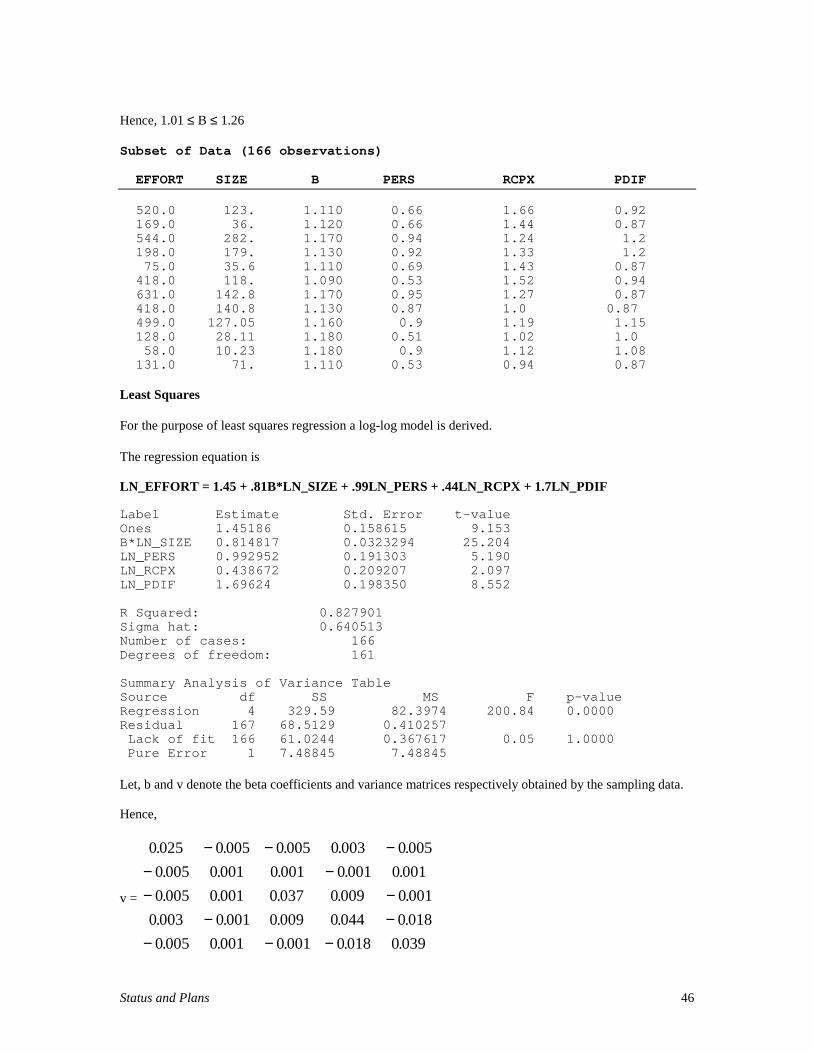
Status and Plans 46
Hence, 1.01 ≤ B ≤ 1.26
Subset of Data (166 observations)
EFFORT SIZE B PERS RCPX PDIF
520.0 123. 1.110 0.66 1.66 0.92 169.0 36. 1.120 0.66 1.44 0.87 544.0 282. 1.170 0.94 1.24 1.2 198.0 179. 1.130 0.92 1.33 1.2 75.0 35.6 1.110 0.69 1.43 0.87 418.0 118. 1.090 0.53 1.52 0.94 631.0 142.8 1.170 0.95 1.27 0.87 418.0 140.8 1.130 0.87 1.0 0.87 499.0 127.05 1.160 0.9 1.19 1.15 128.0 28.11 1.180 0.51 1.02 1.0 58.0 10.23 1.180 0.9 1.12 1.08 131.0 71. 1.110 0.53 0.94 0.87
Least Squares
For the purpose of least squares regression a log-log model is derived.
The regression equation is
LN_EFFORT = 1.45 + .81B*LN_SIZE + .99LN_PERS + .44LN_RCPX + 1.7LN_PDIF
Label Estimate Std. Error t-valueOnes 1.45186 0.158615 9.153B*LN_SIZE 0.814817 0.0323294 25.204LN_PERS 0.992952 0.191303 5.190LN_RCPX 0.438672 0.209207 2.097LN_PDIF 1.69624 0.198350 8.552
R Squared: 0.827901Sigma hat: 0.640513Number of cases: 166Degrees of freedom: 161
Summary Analysis of Variance TableSource df SS MS F p-valueRegression 4 329.59 82.3974 200.84 0.0000Residual 167 68.5129 0.410257 Lack of fit 166 61.0244 0.367617 0.05 1.0000 Pure Error 1 7.48845 7.48845
Let, b and v denote the beta coefficients and variance matrices respectively obtained by the sampling data.
Hence,
v =
0 025 0 005 0 005 0 003 0 005
0 005 0 001 0 001 0 001 0 001
0 005 0 001 0 037 0 009 0 001
0 003 0 001 0 009 0 044 0 018
0 005 0 001 0 001 0 018 0 039
. . . . .
. . . . .
. . . . .
. . . . .
. . . . .
− − −− −− −
− −− − −

Status and Plans 47
and b =
145
081
0 99
0 44
17
.
.
.
.
.
Let, v* and b* denote the beta coefficients and variance matrices respectively obtained by the priorinformation. Suppose,
v* =
0 025 0 0 0 0
0 0 0225 0 001 0 0
0 0 0 025 0 0
0 0 0 0 09 0
0 0 0 0 0 04
.
. .
.
.
.
and b* =
0 92
1
1
1
1
.
The variance for each of the parameter’s beta-coefficients is derived from the assumed standard deviationsas shown in table 4.9.
Table 4.9: Prior Variance for the Beta-coefficientsParameter Standard Deviation Variance
lnA 0.16 0.025B*LN_SIZE 0.15 0.0225
ln(PERS) 0.16 0.025ln(RCPX) 0.3 0.09ln(PDIF) 0.2 0.04
The covariance among the parameters is assumed to be zero. This assumption has been made to simplify theprototype model. In fact, for the complete COCOMO II Bayesian model, this assumption will not be made.Instead, the covariance of the prior will be made equal to the covariance of the sampling data or othertechniques such as the generalized g-prior [Judge85] will be explored.
Since, the rating scale (table 1) used in the regression analysis is the prior information on the parameters,the prior beta coefficients for the parameters, B*Ln_Size, PERS, RCPX and PDIF are 1. And, the prior betacoefficient for lnA is 0.92 (i.e. ln(2.5) since A=2.5 was the value suggested by the COCOMO II affiliatesand COCOMO 81 experience)
Let, v** and b** be the variance and beta coefficients matrices respectively obtained of the posteriorparameters. The xlispstat code shown below was used to obtain these matrices.

Status and Plans 48
> (def x (send L1 :x))X> (def y (send L1 :y))Y> (def xt (transpose x))XT> (def xtx (matmult xt x))XTX> (def xtxinv (inverse xtx))XTXINV
**Or (def xtxinv (send L1:xtxinv))**
> (def xtxinvxt (matmult xtxinv (transpose x)))XTXINVXT> (def b (matmult xtxinvxt y))B> (def bb (bind-rows ’#(1.45186 0.814817 0.992952 0.438672 1.69624))) **make Ba matrix BB**BB> bb#2A((1.45186 0.814817 0.992952 0.438672 1.69624))> (def v1 (bind-rows ’#(0.025 0 0 0 0) ’(0 0.0225 0 0 0) ’(0 0 0.025 0 0) ’(0 00 0.09 0) ’(0 0 0 0 0.04))) **define variance of prior**V1> (def v1inv (inverse v1))V1INV> (def v2inv (+ (matmult (/ 1 (^ (send L1 :sigma-hat) 2)) xtx) v1inv))V2INV> (def v2 (inverse v2inv)) ** define variance of posterior**V2> v2#2A((0.0121329 -0.00222818 0.000987222 0.000367936 -0.00128628) (-0.002228180.000585307 0.000530714 -0.000859041 -3.21192e-05) (0.000987222 0.0005307140.0146764 0.00240605 0.000119682) (0.000367936 -0.000859041 0.00240605 0.0268633-0.00635273) (-0.00128628 -3.21192e-05 0.000119682 -0.00635273 0.0190504))>> (def xty (matmult (transpose x) y))XTY> xty(921.724 4690.38 -257.889 206.246 161.869)> (def xty (bind-columns ’#(921.724 4690.38 -257.889 206.246 161.869)))XTY> (def 1s2xty (matmult (/ 1 (^ (send L1 :sigma-hat) 2)) xty))1S2XTY> v1inv#2A((40 0 0 0 0) (0 44.4444 0 0 0) (0 0 40 0 0) (0 0 0 11.1111 0) (0 0 0 0 25))> (def vv1inv (bind-rows ’(40 0 0 0 0) ’(0 44.4444 0 0 0)’(0 0 40 0 0) ’(0 0 011.1111 0) ’(0 0 0 0 25))) **make v1inv a matrix vv1inv**VV1INV> (def vv1invb1 (matmult vv1inv (bind-columns ’#(0.92 1 1 1 1))))VV1INVB1> (def sum (+ 1S2XTY VV1INVB1))SUM> (def b2 (matmult v2 (+ 1S2XTY VV1INVB1)))B2> b2#2A((1.20034) (0.862394) (0.993368) (0.702535) (1.35215))

Status and Plans 49
Hence,
v** =
0 012 0 002 0 001 0 0004 0 0012
0 002 0 0005 0 0005 0 0008 0
0 001 0 0005 0 015 0 002 0 0001
0 0004 0 0008 0 002 0 027 0 0064
0 0012 0 0 0001 0 0064 0 019
. . . . .
. . . .
. . . . .
. . . . .
. . . .
− −− −
− −− −
and b** =
14
08
10
0 7
13
.
.
.
.
.
The results derived above have been summarized in table 4.10
Table 4.10: Point Estimates and Variances of the Beta CoefficientsPrior Sample Posterior
PointEstimates
(0.92 1 1 1 1) (1.45 0.8 0.99 0.43 1.7 ) (1.2 0.86 0.99 0.7 1.35)
Variance (0.025 0.0225 0.250.09 0.04)
(0.025 0.001 0.0370.044 0.039)
(0.012 0.0005 0.015 0.0270.019)
Note that the posterior variance is the smallest among the three variances for the beta coefficients.
Table 4.11 compares the accuracies of the a-priori and the a-posteriori models
Table 4.11: Improvement in Prediction Accuracies using the Bayesian techniquePrediction Accuracy of SimpleModel
Sampling Data with no priorvariance information
A-Posteriori Model i.e.Sampling data with priorvariance information
PRED(.20) 50/166 = 30% 54/166 = 33%PRED(.30) 68/166 = 41% 74/166 = 45%
Note that there is an increase in prediction accuracy for the a-posteriori model as compared to the modelwith no prior variance information. The full COCOMO II Post Architecture model should give betteraccuracy results due to the addition of more significant parameters such as SITE and SCED. Hence theplans for the completion of this research are:
(i) Collect more data.(ii) Complete the Delphi process to determine a more defensible set of a-priori model parameters.(iii) Perform Bayesian analysis on the complete COCOMO II model.
4.2 Quality Model Current Research Results
Defect Introduction Model
The Defect Introduction model was described in section 3.3.1. The overall Defect Introduction Rate (DIR)of the 1970’s was illustrated as 45 defects/KDSI of which 5/KDSI were Requirements defects, 25/KDSI

Status and Plans 50
were Design defects, 15/KDSI were Coding defects. These DIRs are used as baseline Defect IntroductionRates (DIRBaseline) for the purpose of the model being developed:
Type of Artifact DIRBaseline
Requirements Defects 5/KDSIDesign Defects 25/KDSICoding Defects 15/KDSI
Data is currently being collected from the USC-CSE’s affiliates to help calibrate the model depicted insection 3.3. The results obtained from a sample data point collected are summarized below:
Table 4.12: Defect Introduction Model Current StatusType ofArtifact
1970’sBaseline
DIRs
QualityAdjustment
Factor
PredictedDIR
Actual DIR CalibratedConstant
(A)
1990’sBaseline
DIRsRequirements 5 0.5 2.5 4.5 1.8 9
Design 25 0.44 11 8.4 0.77 19Code 15 0.5 7.5 16.6 2.21 33
These results can be used as the baseline DIRs for the 1990s as shown below.
Type of Artifact DIR Baseline
Requirements Defects 9/KDSIDesign Defects 19/KDSICoding Defects 33/KDSI
But, a lot more data needs to be collected and analyzed to suggest a more stable set of baseline DIRS. Thedata collection is an active ongoing process in the hope of getting as much data as possible.
Defect Removal Model
The Defect Removal Model is being formulated in a similar way as the Defect Introduction model. Abehavioral study of a subset of the COCOMO II parameters to determine the impact of these parameters ondefect removal is being done. Many of the COCOMO II parameters have a direct impact on defect removal.For example, if Required Reliability = Very High, then according to COCOMO II, nearly 40% more effortis expended in developing the software. This is due to the increased attention given to test procedures, QA,CM, documentation, stress testing, integration testing and other defect removal strategies. This increasedeffort could indeed result in nearly 90% of the defects being removed from the product being developed. Onthe other hand, if Required Reliability = Very Low, then according to COCOMO II, only 75% of thenominal effort is required to develop. In this case, very little attention is given to defect removal strategiesand this could remove only 10% of the defects introduced as shown in table 4.13
Table 4.13: Required Software Reliability (RELY)
RELY level Impact on Defect RemovalVH More Requirements defects removed due to more consistency, detailed verification,
QA, CM, standards, SSR, documentation, IV&V interface, test plans, procedures90%
Nominal Nominal level of defect introduction50%
VL Fewer Requirements defects removed due to lower consistency, minimal verification,QA, CM, standards, SSR, documentation, IV&V interface, test plans, procedures
10%Quality Range 10-90%
Similarly the impact of other parameters such as personnel factors, product complexity etc. are beingstudied. Once the model is completely formulated, a 2-round Delphi will be performed to better estimate thedefect removal rates. The plans for the completion of this model are:

Status and Plans 51
(i) Formulate the complete Defect Removal model and complete the Delphi process.(ii) Collect more data and use a bayesian approach similar to that used for COCOMO II.(iii) Integrate the quality model with COCOMO II as shown in figure 4.4
The integrated model can be used to provide insights on determining ship time, assessment of payoffs forquality investments and understanding of interactions amongst quality strategies. Cost, Schedule and Qualityform three sides of the same triangle and this model can play an important role in facilitating the balance ofthe three factors.
The purpose of developing the quality model is to illustrate how the modeling methodology can besuccessfully implemented to develop a strong model in the absence of a lot of data. The problem of the lackof data can be alleviated by expert-judgment based Delphi which determines the impact of the drivers onthe quantity being estimated. A bayesian approach with very strong prior information can be used to modelthe sampling data in the a-posteriori estimation model.
Figure 4.4: Overall Tank and Pipe Quality Model Operation
Software product size estimate
Software product, platformproject, and personnel attributes
Software reuse, maintenance,and increment parameters
Software organization’sproject data
Software development,maintenance cost andschedule estimates
Cost, schedule distributionby phase, activity,increment
COCOMO recalibrated to organization’s data
QualityModel
Software QualityDEFECTS/KDSI OR /FPDefect removal activity levels
COCOMOII
Disciplined Methods

Status and Plans 52

References 53
ReferencesBailey81 - “A Meta-Model for Software Development Resources Expenditures”, Bailey J.W. and Basili V.R., 5th International Conference on Software Engineering, IEEE Press, pp. 107-116.Banker92- , “An Empirical Test of Object-based Output Measurement Metrics in a Computer AidedSoftware Engineering (CASE) Environment”, Rajiv D. Banker, Robert J. Kauffman and Rachna Kumar,1992.Banker94 - “Evidence on Economies of Scale in Software Development”, Rajiv D. Banker, Hsihui Chang,Chris F. Kemerer (1994Information and Software Technology, pp. 275-282.Boehm80 - “Developing Small Scale Application Software Products: Some Experimental Results”, BarryBoehm, Proceedings, IFIP 8th World Computer Congress, 1980.Boehm81 - Software Engineering Economics, Barry W. Boehm, 1981, Prentice-Hall.Boehm95 - “Cost Models for Future Software Life Cycle Processes: COCOMO 2.0”, Boehm, B., B. Clark,E. Horowitz, C. Westland, R. Madachy, R. Selby, 1995, Annals of Software Engineering Special Volumeon Software Process and Product Measurement, J.D. Arthur and S.M. Henry, Eds., J.C. Baltzer AG,Science Publishers, Amsterdam, The Netherlands, Vol. 1, pp. 45 - 60.Briand92 - “A Pattern Recognition Approach for Software Engineering Data Analysis”, Lionel C. Briand,Victor R. Basili and William M. Thomas, IEEE Transactions on Software Engineering, Vol. 18, No. 11,November 1992.Chulani97A - “Calibration Results of COCOMOII.1997”, Sunita Devnani-Chulani, Brad Clark, BarryBoehm, 22nd Software Engineering Workshop, NASA-Goddard, December 1997.Chulani97B - “Modeling Software Defect Introduction”, Sunita Devnani-Chulani, California SoftwareSymposium, November 1997.CSE1 - Center for Software Engineering , “COCOMO II Model Definition Manual,” Computer ScienceDepartment, USC Center for Software Engineering.CSE2 - “Proceedings of the Focused Workshop on Rapid Application Development”, Barry Boehm, SunitaDevnani-Chulani, Alexander Egyed, 1997, USC Center for Software Engineering.Dyer92 - The Cleanroom Approach to Quality Software Development, Michael Dyer, 1992, Wiley Series inSoftware Engineering Practice.Forrester61 - Industrial Dynamics, Cambridge, MA, Forrester J. W., MIT Press, 1961.Forrester68 - Principles of Systems, Cambridge, MA, Forrester J. W., MIT Press, 1968.Frieman79 - “PRICE Software Model. Version 3. An Overview”, Freiman F. R. and Park R. D.,Proceedings of IEEE-PINY Workshop on Quantitative Software Models for Reliability, 1979.Gray97 - “ A Comparison of Techniques for Developing Predictive Models for Software Metrics”, AndrewR. Gray and Stephen G. MacDonnell, Information and Software Technology 39, 1997.Gulezian86 - “Utilizing COCOMO Inputs as a Basis for Developing Generalized Software DevelopmentCost Estimation Model”, Ronald Gulezian, May 1986, COCOMO/WICOMO Users’ Group Meeting, WangInstitute Tyngsboro, MA.Gulledge93 - Analytical Methods in Software Engineering Economics, Thomas R. Gulledge and William P.Hutzler, 1993, Springer-Verlag.Hamid91 - Software Project Dynamics, Abdel-Hamid and Stuart Madnick, Englewood Cliffs, NJ, PrenticeHall 1991.Humphrey95 - A Discipline for Software Engineering, Watts S. Humphrey, 1995, SEI Series in SoftwareEngineering.IFPUG94 - International Function Point Users Group (IFPUG), Function Point Counting practices Manual,Release 4.0, 1994.Jensen84 - “A Comparison of the Jensen and COCOMO Schedule and Cost Estimation Models”, Jensen R.W., Proceedings of the International Society of Parametric Analysis, pp. 96-106.Jones78 - “Measuring Programming Quality and Productivity” by Capers Jones, IBM Systems J., 17, 1,1978, p. 39-63.Jones97 - Applied Software Measurement, Capers Jones, 1997, McGraw Hill.Judge85 - The Theory and Practice of Econometrics, George G. Judge, W. E. Griffiths, R. Carter Hill,Helmut Lutkepohl, Tsoung-Chao Lee, Wiley, 1985.Judge93 - Learning and Practicing Econometrics, George G. Judge, William Griffiths, R. Carter Hill,Wiley, 1993.

References 54
Kemerer87 - “An Empirical Validation of Software Cost Estimation Models”, Chris F. Kemerer,Communications of the ACM, May 1987, Volume 30, Number 5.Khoshgoftaar95 - “Application of Neural Networks for predicting program faults”, T.M. Khoshgoftaar,A.S. Pandya, D.L. Lanning, Annals of Software Engineering, Vol. 1, 1995.Lin92 - “Software Engineering Process Simulation Model”, Lin C., Abdel-Hamid T., Sherif J., TDAProgress Report42-108, JPL, Feb 1992.Madachy94 - “A Software Project Dynamics Model for Process Cost, Schedule and Risk Assessment”,Raymond Madachy, Ph.D. dissertation, USC, 1994.Park88 - “The Central Questions of the PRICE Software Cost Model”, Park R., 4th COCOMO Users’Group Meeting, November 1988.Park92- “Software Size Measurement: A Framework for Counting Source Statements”, Park, 1992CMU-SEI-92-TR-20, Software Engineering Institute, Pittsburg, PA.Poulin97 - Measuring Software Reuse, Principles, Practices and Economic Models, Jeffrey S. Poulin,Addison Wesley, 1997.Putnam92 - Measures for Excellence, Lawrence H, Putnam and Ware Myers, 1992, Yourdon PressComputing Series.Refier89 - Softcost-R, Costar User’s Manual, RCI, 1989.Refier91A - Softcost-Ada, Costar User’s Manual, RCI, 1991.Refier91B - Softcost-)), Costar User’s Manual, RCI, 1991.Revic88 - REVIC Software Cost Estimating Tool, User’s Manual, version 8.0, 1988.Richardson91 - System Dynamics: Simulation Modeling and Analysis, Richardson G. P., Fishwich andLuker, eds., Springer-Verlag.Rubin83 - “Macroestimation of Software Development Parameters: the Estimacs System”, Rubin H.A., inSOFTFAIR Conference Development Tools, Techniques and Alternatives, Arlington, July 1983, IEEEPress, New York, pp.4-16.Shepperd97 - “Estimating Software Project Effort Using Analogies”, M. Shepperd and C. Schofield, IEEETransactions on Software Engineering, Vol. 23, No. 11, November 1997.Stukes94 - “Air Force Cost Analysis Agency Software Model Content Study”, Sherry Stukes and HenryApgar, April 1994.Tausworthe81 - “Deep Space Network Software Cost Estimation Model”, Tausworthe R.C., Jet PropulsionLaboratory Publication 81-7, Pasadena, CA.Thayer78 - Software Reliability, Thomas Thayer, Myron Lipow, Eldred Nelson, North Holland, 1978.Trachtenburg82 - “Discovering how to ensure Software Reliability”, Trachtenburg M., RCA Engineer,Jan/Feb 1982, pp. 53-57.Weisberg85 - Applied Linear Regression, Weisberg, S., 2nd Ed., John Wiley and Sons, New York, N.Y.,1985.Wittig94 - “Using Artificial Neural Networks and Function Points to Estimate 4GL Software DevelopmentEffort”, Wittig G. E. and Finnie G. R., 1994, Australian Journal of Information Systems.

Appendix A 55
Copyright University of Southern California - Version 1.8
Appendix A: COCOMO II Cost Estimation Questionnaire
1. IntroductionThe Center for Software Engineering at the University of Southern California is conducting research to update the softwaredevelopment cost estimation model called COCOMO5. The project name is COCOMO II and is led by Dr. Barry W. Boehm.
A fundamental requirement for such research is real-world software development project data. This data will be used to testhypotheses and verify the model’s postulations. In return the model will be open and made available to the public. Thecontribution of your data will ensure the final model is useful.
The data that is contributed is important to us. We will safeguard your contribution so as not to compromise companyproprietary information. The next section discusses the data management aspects of the project. The following section is thedata collection form. The last section is an explanation of expected values in the data collection form.
Some Affiliates have an active collection program and the data from past projects is available for the COCOMO II datacollection effort. This questionnaire can be used to extract relevant COCOMO II data.
This questionnaire attempts to address two different levels of data granularity: project level and component level. The projectlevel of granularity is data that is applicable for the whole project. This includes things like application type and developmentactivity being reported. Component level data are things like size, cost, and component cost drivers. If the data beingsubmitted is on a project that has multiple components then fill out the project data once, and the component data for each ofthe identifiable component. If the data being submitted for the whole project fill out the form once.
COCOMO II Points of Contact
For questions on USC COCOMO software, the COCOMO II Model, data definitions, or project data collection and management,contact:
Sunita Devnani-Chulani / Brad Clark / Chris Abts (213) 740-6470Jennifer Browning (213) 740-5703Dr. Barry Boehm (213) 740-8163Center for Software Engineering FAX (213) 740-4927Internet Electronic-Mail [email protected]
COCOMO II Data Submission Address:
COCOMO II Data SubmissionCenter for Software EngineeringDepartment of Computer ScienceSalvatori 330University of Southern California941 W. 37th PlaceLos Angeles, CA. 90089-0781
5 Constructive Cost Modeling (COCOMO) is defined in Software Engineering Economics by Barry W. Boehm, Prentice Hall, 1981

Appendix A 56
Copyright University of Southern California - Version 1.8
This Page Left Intentionally Blank

Appendix A 57
Copyright University of Southern California - Version 1.8
2. Project Level Information
General Information
2.1 Affiliate Identification Number. Each separate software project contributing data will have a separate file identification number ofthe form XXX. XXX will be one of a random set of three-digit organization identification numbers, provided by USC Center forSoftware Engineering to the Affiliate.
______________________________
2.2 Project Identification Number. The project identification is a three digit number assigned by the organization. Only the Affiliateknows the correspondence between YYY and the actual project. The same project identification must be used with each datasubmission.
______________________________
2.3 Date prepared. This is the date the data elements were collected for submission.
______________________________
2.4 Application Type. This field captures a broad description of the type of activity this software application is attempting to perform.
Circle One: Command and Control, MIS, Simulation,
Communication, Operating Systems, Software Dev. Tools,
Diagnostics, Process Control, Testing,
Engineering Signal processing, Utilities
and Science
Other:_______________________________
2.5 Activity. This field captures the phase of development that the project is in. For one-time reporting the activity is ‘completed’. It isassumed that data for completed projects includes data from software requirements through integration / test. Please report the correctphasing if this is not the case.
Circle One: Requirements, Design, Code,
Unit Test, Integration/Test, Maintenance,
Completed
Other:_______________________________
2.6 Development Type.
Is the development a new software product or an upgrade of an existing product?
2.7 Development Process. This is a description of the software process used to control the software development.
______________________________
2.8 Development Process Iteration. If the process is iterative, e.g. spiral, which iteration is this?
______________________________
Circle One: New Product Upgrade

Appendix A 58
Copyright University of Southern California - Version 1.8
2.9 COCOMO Model. This specifies which COCOMO II model is being used in this data submission. If this is a "historical" datasubmission, select the Post-Architecture model or the Applications Composition model.
• Application Composition: This model involves prototyping efforts to resolve potential high risk issues such as user interfaces,software/system interaction, performance, or technology maturity.
• Early Design: This model involves exploration of alternative software/system architectures and concepts of operations. At thisstage of development, not enough is known to support fine-grain cost estimation.
• Post-Architecture: This model involves the actual development and maintenance of a software product. This stage ofdevelopment proceeds most cost-effectively if a software life-cycle architecture has been developed; validated with respect tothe system’s mission, concept of operation, and risk; and established as the framework for the product.
Circle One: Application Composition, Early Design, Post-Architecture
2.10 Success Rating for Project. This specifies the degree of success for the project.
• Very successful; did almost everything right
• Successful; did the big things right
• OK; stayed out of trouble
• Some Problems; took some effort to keep viable
• Major Problems; would not do this project again
Schedule
2.11 Year of development. For reporting of historical data, please provide the year in which the software development was completed.For periodic reporting put the year of this submission or leave blank.
______________________________
Circle One: Very Successful Successful OK Some Problems Major Problems

Appendix A 59
Copyright University of Southern California - Version 1.8
2.12 Schedule Months. For reporting of historical data, provide the number of calendar months from the time the development beganthrough the time it completed (from the beginning of Software Preliminary Design through the end of System Test and Integration).For periodic reporting, provide the number of months in this development activity.
Circle the life-cycle phases that the schedule covers:
SystemRequirements
SoftwareRequirements
PreliminaryDesign
DetailedDesign
Code andUnit Test
Integrationand Test
Maintenance
• Software Requirements. This phase defines the complete, validated specification of the required functions, interfaces, andperformances for the software product.
• Preliminary Design. This phase defines the complete, verified specification of the overall hardware/software architecture,control structure, and data structure for the product, along with such necessary components as draft user’s manuals and testplans.
• Detailed Design. This phase defines a complete, verified specification of the control structure, data structure, interfacerelations, sizing, key algorithms, and assumptions of each program component.
• Code & Unit Test. This phase produces a complete and verified set of program components.
• S/W System Integration & Test. This phase produces a properly functioning software product composed of the softwarecomponents.
• Maintenance. This phase produces a fully functioning update of the hardware/software system.
Project Exponential Cost Drivers
Scale Factors(Wi)
Very Low Low Nominal High Very High Extra High
Precedentedness thoroughlyunprecedented
largelyunprecedented
somewhatunprecedented
generally familiar largely familiar thoroughlyfamiliar
DevelopmentFlexibility
rigorous occasionalrelaxation
some relaxation general conformity some conformity general goals
Architecture / riskresolutiona.
little (20%) some (40%) often (60%) generally (75%) mostly (90%) full (100%)
Team cohesionvery difficultinteractions
some difficultinteractions
basicallycooperativeinteractions
largely cooperative highly cooperative seamlessinteractions
a.% significant module interfaces specified, % significant risks eliminated.
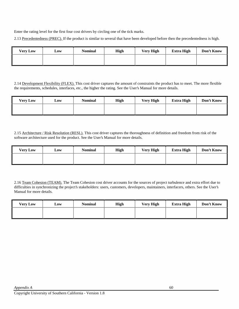
Appendix A 60
Copyright University of Southern California - Version 1.8
Enter the rating level for the first four cost drivers by circling one of the tick marks.
2.13 Precedentedness (PREC). If the product is similar to several that have been developed before then the precedentedness is high.
Very Low Low Nominal High Very High Extra High Don’t Know
2.14 Development Flexibility (FLEX). This cost driver captures the amount of constraints the product has to meet. The more flexiblethe requirements, schedules, interfaces, etc., the higher the rating. See the User’s Manual for more details.
Very Low Low Nominal High Very High Extra High Don’t Know
2.15 Architecture / Risk Resolution (RESL). This cost driver captures the thoroughness of definition and freedom from risk of thesoftware architecture used for the product. See the User’s Manual for more details.
Very Low Low Nominal High Very High Extra High Don’t Know
2.16 Team Cohesion (TEAM). The Team Cohesion cost driver accounts for the sources of project turbulence and extra effort due todifficulties in synchronizing the project’s stakeholders: users, customers, developers, maintainers, interfacers, others. See the User’sManual for more details.
Very Low Low Nominal High Very High Extra High Don’t Know

Appendix A 61
Copyright University of Southern California - Version 1.8
2.17 Process Maturity (PMAT). The procedure for determining PMAT is organized around the Software Engineering Institute’sCapability Maturity Model (CMM). The time period for reporting process maturity is at the time the project was underway. We areinterested in the capabilities practiced at the project level more than the overall organization’s capabilities. There are three ways ofresponding to this question: choose only one. "Key Process Area Evaluation" requires a response for each Key Process Area (KPA).We have provided enough information for you to self-evaluate the project’s enactment of a KPA (we hope will you will take the time tocomplete this section). "Overall Maturity Level" is a response that captures the result of an organized evaluation based on the CMM."No Response" means you do not know or will not report the process maturity either at the Capability Maturity Model or Key ProcessArea level.
r No Response
Overall Maturity Level
r CMM Level 1 (lower half)
r CMM Level 1 (upper half)
r CMM Level 2
r CMM Level 3
r CMM Level 4
r CMM Level 5
Basis of estimate:
r Software Process Assessment (SPA)
r Software Capability Evaluation (SCE)
r Interim Process Assessment (IPA)
r Other: ___________________________________
Key Process Area Evaluation
Enough information is provided in the following table so that you can assess the degree to which a KPA was exercised on the project.Each KPA is briefly described and its goals are given. The response categories are explained below:
• Almost Always (over 90% of the time) when the goals are consistently achieved and are well established in standardoperating procedures.
• Frequently (about 60 to 90% of the time) when the goals are achieved relatively often, but sometimes are omitted underdifficult circumstances.
• About Half (about 40 to 60% of the time) when the goals are achieved about half of the time.
• Occasionally (about 10 to 40% of the time) when the goals are sometimes achieved, but less often.
• Rarely If Ever (less than 10% of the time) when the goals are rarely if ever achieved.
• Does Not Apply when you have the required knowledge about your project or organization and the KPA, but you feel theKPA does not apply to your circumstances (e.g. Subcontract Management).
• Don’t Know when you are uncertain about how to respond for the KPA.

Appendix A 62
Copyright University of Southern California - Version 1.8
Key Process Area Goals of each KPAAlmostAlways
Frequently AboutHalf
Occasionally RarelyIf Ever
Does NotApply
Don’tKnow
Requirements Management: involvesestablishing and maintaining an agreement withthe customer on the requirements for thesoftware project.
System requirements allocated to software arecontrolled to establish a baseline for softwareengineering and management use. Software plans,products, and activities are kept consistent with thesystem requirements allocated to software.
r r r r r r r
Software Project Planning: establishesreasonable plans for performing the softwareengineering activities and for managing thesoftware project.
Software estimates are documented for use in planningand tracking the software project. Software projectactivities and commitments are planned anddocumented. Affected groups and individuals agree totheir commitments related to the software project.
r r r r r r r
Software Project Tracking and Oversight:provides adequate visibility into actual progressso that management can take corrective actionswhen the software project’s performance deviatessignificantly from the software plans.
Actual results and performances are tracked against thesoftware plans. Corrective actions are taken andmanaged to closure when actual results andperformance deviate significantly from the softwareplans. Changes to software commitments are agreed toby the affected groups and individuals.
r r r r r r r
Software Subcontract Management: involvesselecting a software subcontractor, establishingcommitments with the subcontractor, andtracking and reviewing the subcontractor’sperformance and results.
The prime contractor selects qualified softwaresubcontractors. The prime contractor and the softwaresubcontractor agree to their commitments to each other.The prime contractor and the software subcontractormaintain ongoing communications. The primecontractor tracks the software subcontractor’s actualresults and performance against its commitments.
r r r r r r r
Software Quality Assurance: providesmanagement with appropriate visibility into theprocess being used by the software project and ofthe products being built.
Software quality assurance activities are planned.Adherence of software products and activities to theapplicable standards, procedures, and requirements isverified objectively. Affected groups and individualsare informed of software quality assurance activitiesand results. Noncompliance issues that cannot beresolved within the software project are addressed bysenior management.
r r r r r r r
Software Configuration Management: establishesand maintains the integrity of the products of thesoftware project throughout the project’s softwarelife cycle.
Software configuration management activities areplanned. Selected software work products areidentified, controlled, and available. Changes toidentified software work products are controlled.Affected groups and individuals are informed of the
r r r r r r r

Appendix A 63
Copyright University of Southern California - Version 1.8
Key Process Area Goals of each KPAAlmostAlways
Frequently AboutHalf
Occasionally RarelyIf Ever
Does NotApply
Don’tKnow
status and content of software baselines.
Organization Process Focus: establishes theorganizational responsibility for software processactivities that improve the organization’s overallsoftware process capability.
Software process development and improvementactivities are coordinated across the organization. Thestrengths and weaknesses of the software processesused are identified relative to a process standard.Organization-level process development andimprovement activities are planned.
r r r r r r r
Organization Process Definition: develops andmaintains a usable set of software process assetsthat improve process performance across theprojects and provides a basis for cumulative,long- term benefits to the organization.
A standard software process for the organization isdeveloped and maintained. Information related to theuse of the organization’s standard software process bythe software projects is collected, reviewed, and madeavailable.
r r r r r r r
Training Program: develops the skills andknowledge of individuals so they can performtheir roles effectively and efficiently.
Training activities are planned. Training for developingthe skills and knowledge needed to perform softwaremanagement and technical roles is provided.Individuals in the software engineering group andsoftware-related groups receive the training necessaryto perform their roles.
r r r r r r r
Integrated Software Management: integrates thesoftware engineering and management activitiesinto a coherent, defined software process that istailored from the organization’s standard softwareprocess and related process assets.
The project’s defined software process is a tailoredversion of the organization’s standard software process.The project is planned and managed according to theproject’s defined software process.
r r r r r r r
Software Product Engineering: integrates all thesoftware engineering activities to produce andsupport correct, consistent software productseffectively and efficiently.
The software engineering tasks are defined, integrated,and consistently performed to produce the software.Software work products are kept consistent with eachother.
r r r r r r r
Intergroup Coordination: establishes a means forthe software engineering group to participateactively with the other engineering groups so theproject is better able to satisfy the customer’sneeds effectively and efficiently.
The customer’s requirements are agreed to by allaffected groups. The commitments between theengineering groups are agreed to by the affectedgroups. The engineering groups identify, track, andresolve intergroup issues.
r r r r r r r
Peer Review: removes defects from the softwarework products early and efficiently.
Peer review activities are planned. Defects in thesoftware work products are identified and removed.
r r r r r r r
Quantitative Process Management: controls the The quantitative process management activities are
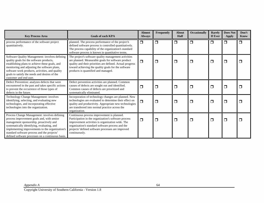
Appendix A 64
Copyright University of Southern California - Version 1.8
Key Process Area Goals of each KPAAlmostAlways
Frequently AboutHalf
Occasionally RarelyIf Ever
Does NotApply
Don’tKnow
process performance of the software projectquantitatively.
planned. The process performance of the project’sdefined software process is controlled quantitatively.The process capability of the organization’s standardsoftware process is known in quantitative terms.
r r r r r r r
Software Quality Management: involves definingquality goals for the software products,establishing plans to achieve these goals, andmonitoring and adjusting the software plans,software work products, activities, and qualitygoals to satisfy the needs and desires of thecustomer and end user.
The project’s software quality management activitiesare planned. Measurable goals for software productquality and their priorities are defined. Actual progresstoward achieving the quality goals for the softwareproducts is quantified and managed.
r r r r r r r
Defect Prevention: analyzes defects that wereencountered in the past and takes specific actionsto prevent the occurrence of those types ofdefects in the future.
Defect prevention activities are planned. Commoncauses of defects are sought out and identified.Common causes of defects are prioritized andsystematically eliminated.
r r r r r r r
Technology Change Management: involvesidentifying, selecting, and evaluating newtechnologies, and incorporating effectivetechnologies into the organization.
Incorporation of technology changes are planned. Newtechnologies are evaluated to determine their effect onquality and productivity. Appropriate new technologiesare transferred into normal practice across theorganization.
r r r r r r r
Process Change Management: involves definingprocess improvement goals and, with seniormanagement sponsorship, proactively andsystematically identifying, evaluating, andimplementing improvements to the organization’sstandard software process and the projects’defined software processes on a continuous basis.
Continuous process improvement is planned.Participation in the organization’s software processimprovement activities is organization wide. Theorganization’s standard software process and theprojects’ defined software processes are improvedcontinuously.
r r r r r r r

Appendix A 65
Copyright University of Southern California - Version 1.8
2.18 Severity of Defects. Categorize the several defects based on their severity using the followingclassification6 information:
• Critical
Causes a system crash or unrecoverable data loss or jeopardizes personnel.
The product is unusable (and in mission/safety software would prevent the completion of themission).
• High
Causes impairment of critical system functions and no workaround solution exists.
Some aspects of the product do not work ( and the defect adversely affects successful completionof mission in mission/safety software), but some attributes do work in its current situation.
• Medium
Causes impairment of critical system function, though a workaround solution does exist.
The product can be used, but a workaround (from a customer’s preferred method of operation)must be used to achieve some capabilities. The presence of medium priority defects usuallydegrades the work.
• Low
Causes a low level of inconvenience or annoyance.
The product meets its requirements and can be used with just a little inconvenience. Typos indisplays such as spelling, punctuation, and grammar which generally do not cause operationalproblems are usually categorized as low severity.
• None
Concerns a duplicate or completely trivial problem, such as a minor typo in supportingdocumentation.
Critical and High severity defects result in an approved change request or failure report.
6 Adapted from IEEE Std 1044.1-1995
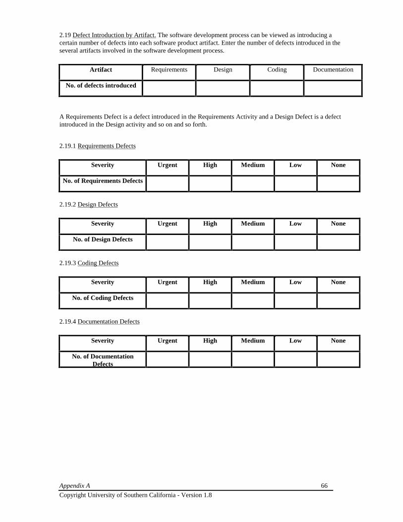
Appendix A 66
Copyright University of Southern California - Version 1.8
2.19 Defect Introduction by Artifact. The software development process can be viewed as introducing acertain number of defects into each software product artifact. Enter the number of defects introduced in theseveral artifacts involved in the software development process.
Artifact Requirements Design Coding Documentation
No. of defects introduced
A Requirements Defect is a defect introduced in the Requirements Activity and a Design Defect is a defectintroduced in the Design activity and so on and so forth.
2.19.1 Requirements Defects
Severity Urgent High Medium Low None
No. of Requirements Defects
2.19.2 Design Defects
Severity Urgent High Medium Low None
No. of Design Defects
2.19.3 Coding Defects
Severity Urgent High Medium Low None
No. of Coding Defects
2.19.4 Documentation Defects
Severity Urgent High Medium Low None
No. of DocumentationDefects

Appendix A 67
Copyright University of Southern California - Version 1.8
2.20 Defect Removal by Activity.
2.20.1 Requirements Defects
Enter the number of Requirements Defects that were removed in the several activities involved in thesoftware development process.
Activity Requirements Design Coding Documentation Testing
No. of Requirements Defectsremoved
2.20.2 Design Defects
Enter the number of Design Defects that were removed in the several activities involved in the softwaredevelopment process.
Activity Design Coding Documentation Testing
No. of Design Defectsremoved
2.20.3 Coding Defects
Enter the number of Coding Defects that were discovered in the several activities removed in the softwaredevelopment process.
Activity Design Coding Documentation Testing
No. of Coding Defectsremoved
2.20.4 Documentation Defects
Enter the number of Documentation Defects that were removed in the several activities involved in thesoftware development process.
Activity Design Coding Documentation Testing
No. of DocumentationDefects removed
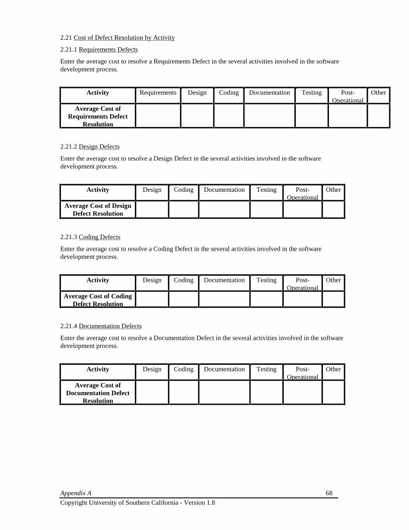
Appendix A 68
Copyright University of Southern California - Version 1.8
2.21 Cost of Defect Resolution by Activity
2.21.1 Requirements Defects
Enter the average cost to resolve a Requirements Defect in the several activities involved in the softwaredevelopment process.
Activity Requirements Design Coding Documentation Testing Post-Operational
Other
Average Cost ofRequirements Defect
Resolution
2.21.2 Design Defects
Enter the average cost to resolve a Design Defect in the several activities involved in the softwaredevelopment process.
Activity Design Coding Documentation Testing Post-Operational
Other
Average Cost of DesignDefect Resolution
2.21.3 Coding Defects
Enter the average cost to resolve a Coding Defect in the several activities involved in the softwaredevelopment process.
Activity Design Coding Documentation Testing Post-Operational
Other
Average Cost of CodingDefect Resolution
2.21.4 Documentation Defects
Enter the average cost to resolve a Documentation Defect in the several activities involved in the softwaredevelopment process.
Activity Design Coding Documentation Testing Post-Operational
Other
Average Cost ofDocumentation Defect
Resolution
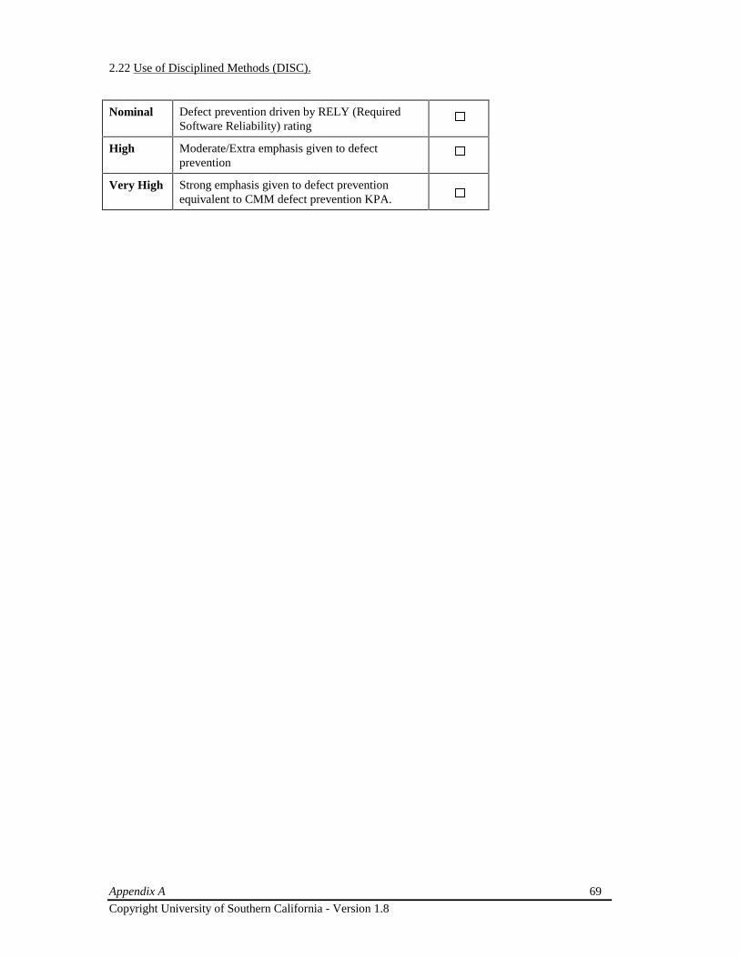
Appendix A 69
Copyright University of Southern California - Version 1.8
2.22 Use of Disciplined Methods (DISC).
Nominal Defect prevention driven by RELY (RequiredSoftware Reliability) rating
High Moderate/Extra emphasis given to defectprevention
Very High Strong emphasis given to defect preventionequivalent to CMM defect prevention KPA.

Appendix A 70
Copyright University of Southern California - Version 1.8
3. Component Level Information
Component ID
If the whole project is being reported as a single component then skip to the next section.
If the data being submitted is for multiple components that comprise a single project then it isnecessary to identify each component with its project. Please fill out this section for eachcomponent and attach all of the component sections to the project sections describing the overallproject data.
3.1 Affiliate Identification Number. Each separate software project contributing data will have a separatefile identification number of the form XXX. XXX will be one of a random set of three-digit organizationidentification numbers, provided by USC Center for Software Engineering to the Affiliate.
______________________________
3.2 Project Identification Number. The project identification is a three digit number assigned by theorganization. Only the Affiliate knows the correspondence between YYY and the actual project. The sameproject identification must be used with each data submission.
______________________________
3.3 Component Identification (if applicable). This is a unique sequential letter that identifies a softwaremodule that is part of a project.
Circle One: A B C D E F G H I
J K L M N O P Q R
Cost
3.4 Total Effort (Person Months). For one-time reporting, provide the effort in Person Months associatedwith development and test of the software component described, including its share of such commonactivities as system design and integration. For periodic reporting, provide the effort in Person Months sincethe project began.
______________________________
Circle the life-cycle phases that the effort estimate covers:
SystemRequirements
SoftwareRequirements
PreliminaryDesign
DetailedDesign
Code andUnit Test
Integrationand Test
Maintenance
3.5 Hours / Person Month. Indicate the average number of hours per person month experienced by yourorganization.
______________________________

Appendix A 71
Copyright University of Southern California - Version 1.8
3.6 Labor Breakout. Indicate the percentage of labor for different categories,e.g. Managers, S/WRequirement Analysts, Designers, CM/QA Personnel, Programmers, Testers, and Interfacers for each phaseof software development:
Labor CategoryTotalfor allphases
Rqts PD DD CUT IT M
• Requirements(Rqts). This phase defines the complete, validated specification of the requiredfunctions, interfaces, and performances for the software product.
• Preliminary Design (PD). This phase defines the complete, verified specification of the overallhardware/software architecture, control structure, and data structure for the product, along withsuch necessary components as draft user’s manuals and test plans.
• Detailed Design (DD). This phase defines a complete, verified specification of the controlstructure, data structure, interface relations, sizing, key algorithms, and assumptions of eachprogram component.
• Code & Unit Test (CUT). This phase produces a complete and verified set of programcomponents.
• S/W System Integration & Test (IT). This phase produces a properly functioning software productcomposed of the software components.
• Maintenance (M). This phase produces a fully functioning update of the hardware/software system.
Size
The project would like to collect size in object points, logical lines of code, and unadjustedfunction points. Please submit all size measures that are available, e.g. if you have a component inlines of code and unadjusted function points then submit both numbers.
3.7 Percentage of Code Breakage. This is an estimate of how much the requirements have changed over thelifetime of the project. It is the percentage of code thrown away due to requirements volatility. For example,a project which delivers 100,000 instructions but discards the equivalent of an additional 20,000instructions would have a breakage of value of 20. See the User’s Manual for more detail.
______________________________
3.8 Object Points. If the COCOMO II Applications Programming model was used then enter the objectpoint count.
______________________________

Appendix A 72
Copyright University of Southern California - Version 1.8
3.9 New Unique SLOC. This is the number of new source lines of code (SLOC) generated.
______________________________
3.10 SLOC Count Type. When reporting size in source lines of code, please indicate if the count was forlogical SLOC or physical SLOC. If both are available, please submit both types of counts. If neither type ofcount applies to the way the code was counted, please describe the method. An extensive definition forlogical source lines of code is given in an Appendix in the Model User’s Manual.
Circle One: Logical SLOC Physical SLOC (carriage returns)
Physical SLOC (semicolons) Non-Commented/Non-Blank SLOC
Other: __________________________________________________________
3.11 Unadjusted Function Points. If you are using the Early Design or Post-Architecture model, provide thetotal Unadjusted Function Points for each type. An Unadjusted Function Point is the product of the functionpoint count and the weight for that type of point. Function Points are discussed in the User’s Manual.
______________________________
3.12 Programming Language. If you are using the Early Design or Post-Architecture model, enter thelanguage name that was used in this component, e.g. Ada, C, C++, COBOL, FORTRAN and the amount ofusage if more than one language was used.
Language Used Percentage Used
3.13 Software Maintenance Parameters. For software maintenance, use items 3.8 - 3.12 to describe the sizeof the base software product, and use the same units to describe the following parameters:
a. Amount of software added: ____________________________
b. Amount of software modified: _________________________
c. Amount of software deleted: ___________________________

Appendix A 73
Copyright University of Southern California - Version 1.8
3.14 Object Points Reused. If you are using the Application Composition model, enter the number of objectpoints reused. Do not fill in the fields on DM, CM, IM, SU, or AA.
______________________________
3.15 ASLOC Adapted. If you are using the Early Design or Post-Architecture model enter the amounts forthe SLOC adapted.
______________________________
3.16 ASLOC Count Type. When reporting size in source lines of code, please indicate if the count was forlogical ASLOC or physical ASLOC. If both are available, please submit both types of counts. If neithertype of count applies to the way the code was counted, please describe the method. An extensive definitionfor logical source lines of code is given in an Appendix in the Model User’s Manual.
Circle One: Logical ASLOC Physical ASLOC (carriage returns)
Physical ASLOC (semicolons) Non-Commented/Non-Blank ASLOC
Other: __________________________________________________________
3.17 Design Modified - DM. The percentage of design modified.
______________________________
3.18 Code Modified - CM. The percentage of code modified.
______________________________
3.19 Integration and Test - IM. The percentage of the adapted software’s original integration and test effortexpended.
______________________________
3.20 Software Understanding - SU.
Very Low Low Nom High Very High
Structure Very lowcohesion, highcoupling, spaghetticode.
Moderately lowcohesion, highcoupling.
Reasonably well-structured; someweak areas.
High cohesion,low coupling.
Strong modularity,information hidingin data / controlstructures.
ApplicationClarity
No match betweenprogram andapplication worldviews.
Some correlationbetween programand application.
Moderatecorrelationbetween programand application.
Good correlationbetween programand application.
Clear matchbetween programand applicationworld-views.
Self-Descriptiveness Obscure code;documentationmissing, obscureor obsolete
Some codecommentary andheaders; someusefuld t ti
Moderate level ofcode commentary,headers,documentations.
Good codecommentary andheaders; usefuldocumentation;
k
Self-descriptivecode;documentation up-to-date, well-
i d ithSU Increment to ESLOC 50 40 30 20 10
Table 1: Rating Scale for Software Understanding Increment SU

Appendix A 74
Copyright University of Southern California - Version 1.8
The Software Understanding increment (SU) is obtained from Table 1. SU is expressed quantitatively as apercentage. If the software is rated very high on structure, applications clarity, and self-descriptiveness, thesoftware understanding and interface checking penalty is 10%. If the software is rated very low on thesefactors, the penalty is 50%. SU is determined by taking the subjective average of the three categories. Enterthe percentage.
3.21 Assessment and Assimilation - AA.
AA Increment Level of AA Effort
0 None2 Basic module search and documentation
4 Some module Test and Evaluation (T&E), documentation
6 Considerable module T&E, documentation
8 Extensive module T&E, documentation
Table 2: Rating Scale for Assessment and Assimilation Increment (AA)
The other nonlinear reuse increment deals with the degree of Assessment and Assimilation (AA) needed todetermine whether a fully-reused software module is appropriate to the application, and to integrate itsdescription into the overall product description. Table 2 provides the rating scale and values for theassessment and assimilation increment. Enter the percentage of AA:
3.22 Programmer Unfamiliarity - UNFM.
UNFM Increment Level of Unfamiliarity
0.0 Completely familiar0.2 Mostly familiar
0.4 Somewhat familiar
0.6 Considerably familiar
0.8 Mostly unfamiliar
1.0 Completely unfamiliar
Table 3: Rating Scale for Programmer Unfamiliarity (UNFM)
The amount of effort required to modify existing software is a function not only of the amount ofmodification (AAF) and understandability of the existing software (SU), but also of the programmer’srelative unfamiliarity with the software (UNFM). The UNFM parameter is applied multiplicatively to thesoftware understanding effort increment. If the programmer works with the software every day, the 0.0multiplier for UNFM will add no software understanding increment. If the programmer has never seen thesoftware before, the 1.0 multiplier will add the full software understanding effort increment. The rating ofUNFM is in Table 3. Enter the Level of Unfamiliarity.

Appendix A 75
Copyright University of Southern California - Version 1.8
Post-Architecture Cost Drivers.
Use this section for completed projects. These are the 17 effort multipliers used in COCOMO II Post-Architecture model to adjust the nominal effort, Person Months, to reflect the software product underdevelopment. They are grouped into four categories: product, platform, personnel, and project. When anevaluation is in-between two rating levels always round to Nominal.
Product Cost Drivers.
For maintenance projects, identify any differences between the base code and modified code Product CostDrivers (e.g. complexity).
Very Low Low Nominal High Very High Extra High
RELY slightinconvenience
low, easilyrecoverable losses
moderate, easilyrecoverable losses
high financialloss
risk to human life
DATA DB bytes/Pgm SLOC< 10
10 < D/P < 100 100 < D/P < 1000 D/P > 1000
RUSE none across project across program across product line across multipleproduct lines
DOCU Many life-cycleneeds uncovered
Some life-cycle needsuncovered.
Right-sized to life-cycle needs
Excessive for life-cycle needs
Very excessive forlife-cycle needs
3.23 Required Software Reliability (RELY). This is the measure of the extent to which the software mustperform its intended function over a period of time.
Very Low Low Nominal High Very High Don’t Know
3.24 Data Base Size (DATA). This measure attempts to capture the affect large data requirements have onproduct development. The rating is determined by calculating D/P.
Low Nominal High Very High Don’t Know
3.25 Required Reusability(RUSE). This cost driver accounts for the additional effort needed to constructcomponents intended for reuse on the current or future projects.
Low Nominal High Very High Don’t Know

Appendix A 76
Copyright University of Southern California - Version 1.8
3.26 Documentation match to life-cycle needs (DOCU). This captures the suitability of the project’sdocumentation to its life-cycle needs. See the User’s Manual.
Very Low Low Nominal High Very High Don’t Know
3.27 Product Complexity (CPLX):
Control Operations ComputationalOperations
Device-dependentOperations
Data ManagementOperations
User InterfaceManagementOperations
Very Low Straight-line code with a fewnon-nested structuredprogramming operators: DOs,CASEs, IFTHENELSEs. Simplemodule composition viaprocedure calls or simple scripts.
Evaluation of simpleexpressions: e.g.,A=B+C*(D-E)
Simple read, writestatements withsimple formats.
Simple arrays in mainmemory. SimpleCOTS-DB queries,updates.
Simple inputforms, reportgenerators.
Low Straightforward nesting ofstructured programmingoperators. Mostly simplepredicates
Evaluation of moderate-level expressions: e.g.,D=SQRT(B**2-4.*A*C)
No cognizance neededof particular processoror I/O devicecharacteristics. I/Odone at GET/PUTlevel.
Single file subsettingwith no data structurechanges, no edits, nointermediate files.Moderately complexCOTS-DB queries,updates.
Use of simplegraphic userinterface (GUI)builders.
Nominal Mostly simple nesting. Someintermodule control. Decisiontables. Simple callbacks ormessage passing, includingmiddleware-supporteddistributed processing
Use of standard math andstatistical routines. Basicmatrix/vector operations.
I/O processingincludes deviceselection, statuschecking and errorprocessing.
Multi-file input andsingle file output.Simple structuralchanges, simple edits.Complex COTS-DBqueries, updates.
Simple use ofwidget set.
High Highly nested structuredprogramming operators withmany compound predicates.Queue and stack control.Homogeneous, distributedprocessing. Single processor softreal-time control.
Basic numerical analysis:multivariate interpolation,ordinary differentialequations. Basictruncation, roundoffconcerns.
Operations at physicalI/O level (physicalstorage addresstranslations; seeks,reads, etc.). OptimizedI/O overlap.
Simple triggersactivated by datastream contents.Complex datarestructuring.
Widget setdevelopment andextension. Simplevoice I/O,multimedia.
Very High Reentrant and recursive coding.Fixed-priority interrupt handling.Task synchronization, complexcallbacks, heterogeneousdistributed processing. Single-processor hard real-time control.
Difficult but structurednumerical analysis: near-singular matrix equations,partial differentialequations. Simpleparallelization.
Routines for interruptdiagnosis, servicing,masking.Communication linehandling.Performance-intensiveembedded systems.
Distributed databasecoordination. Complextriggers. Searchoptimization.
Moderatelycomplex 2D/3D,dynamic graphics,multimedia.
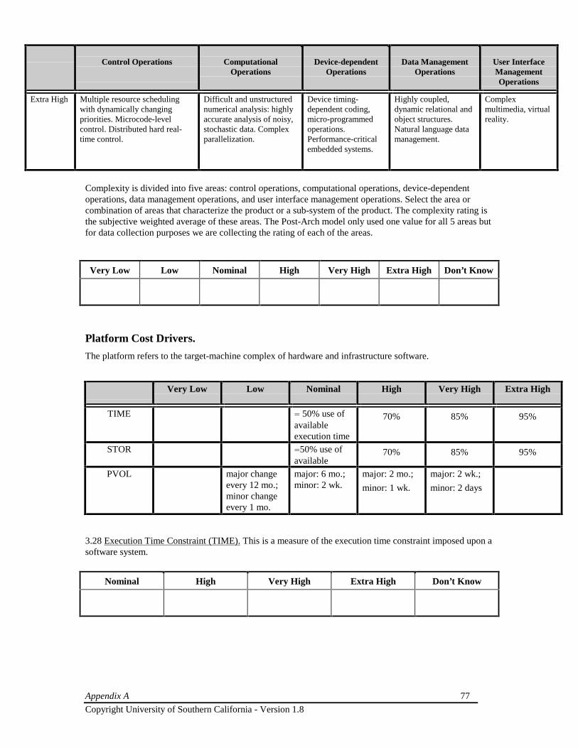
Appendix A 77
Copyright University of Southern California - Version 1.8
Control Operations ComputationalOperations
Device-dependentOperations
Data ManagementOperations
User InterfaceManagementOperations
Extra High Multiple resource schedulingwith dynamically changingpriorities. Microcode-levelcontrol. Distributed hard real-time control.
Difficult and unstructurednumerical analysis: highlyaccurate analysis of noisy,stochastic data. Complexparallelization.
Device timing-dependent coding,micro-programmedoperations.Performance-criticalembedded systems.
Highly coupled,dynamic relational andobject structures.Natural language datamanagement.
Complexmultimedia, virtualreality.
Complexity is divided into five areas: control operations, computational operations, device-dependentoperations, data management operations, and user interface management operations. Select the area orcombination of areas that characterize the product or a sub-system of the product. The complexity rating isthe subjective weighted average of these areas. The Post-Arch model only used one value for all 5 areas butfor data collection purposes we are collecting the rating of each of the areas.
Very Low Low Nominal High Very High Extra High Don’t Know
Platform Cost Drivers.
The platform refers to the target-machine complex of hardware and infrastructure software.
Very Low Low Nominal High Very High Extra High
TIME = 50% use ofavailableexecution time
70% 85% 95%
STOR =50% use ofavailable
70% 85% 95%
PVOL major changeevery 12 mo.;minor changeevery 1 mo.
major: 6 mo.;minor: 2 wk.
major: 2 mo.;
minor: 1 wk.
major: 2 wk.;
minor: 2 days
3.28 Execution Time Constraint (TIME). This is a measure of the execution time constraint imposed upon asoftware system.
Nominal High Very High Extra High Don’t Know

Appendix A 78
Copyright University of Southern California - Version 1.8
3.29 Main Storage Constraint (STOR). This rating represents the degree of main storage constraint imposedon a software system or subsystem. See the User’s Manual.
Nominal High Very High Extra High Don’t Know
3.30 Platform Volatility (PVOL). "Platform" is used here to mean the complex of hardware and software(OS, DBMS, etc.) the software product calls on to perform its tasks.
Low Nominal High Very High Don’t Know
Personnel Cost Drivers.
Very Low Low Nominal High Very High Extra High
ACAP 15th percentile 35th percentile 55th percentile 75th percentile 90th percentilePCAP 15th percentile 35th percentile 55th percentile 75th percentile 90th percentile
PCON 48% / year 24% / year 12% / year 6% / year 3% / year
AEXP = 2 months 6 months 1 year 3 years 6 years
PEXP = 2 months 6 months 1 year 3 years 6 year
LTEX = 2 months 6 months 1 year 3 years 6 year
3.31 Analyst Capability (ACAP). Analysts are personnel that work on requirements, high level design anddetailed design. See the User’s Manual.
Very Low Low Nominal High Very High Don’t Know
3.32 Programmer Capability (PCAP). Evaluation should be based on the capability of the programmers as ateam rather than as individuals. Major factors which should be considered in the rating are ability,efficiency and thoroughness, and the ability to communicate and cooperate. See the User’s Manual.
Very Low Low Nominal High Very High Don’t Know

Appendix A 79
Copyright University of Southern California - Version 1.8
3.33 Applications Experience (AEXP). This rating is dependent on the level of applications experience ofthe project team developing the software system or subsystem. The ratings are defined in terms of theproject team’s equivalent level of experience with this type of application. See the User’s Manual.
Very Low Low Nominal High Very High Don’t Know
3.34 Platform Experience (PEXP). The Post-Architecture model broadens the productivity influence ofPEXP, recognizing the importance of understanding the use of more powerful platforms, including moregraphic user interface, database, networking, and distributed middleware capabilities. See the User’sManual.
Very Low Low Nominal High Very High Don’t Know
3.35 Language and Tool Experience (LTEX). This is a measure of the level of programming language andsoftware tool experience of the project team developing the software system or subsystem. See the User’sManual.
Very Low Low Nominal High Very High Don’t Know
3.36 Personnel Continuity (PCON). The rating scale for PCON is in terms of the project’s annual personnelturnover.
Very Low Low Nominal High Very High Don’t Know
Project Cost Drivers.
This table gives a summary of the criteria used to select a rating level for project cost drivers.
Very Low Low Nominal High Very High Extra High
TOOL edit, code, debug simple, frontend,backend CASE,little integration
basic lifecycletools,moderatelyintegrated
strong, maturelifecycle tools,moderatelyintegrated
strong, mature,proactivelifecycle tools,well integrated
SITE:Collocation
International Multi-city andMulti-company
Multi-city orMulti-company
Same city ormetro. area
Same buildingor complex
Fully collocated
SITE:Communications
Some phone,mail
Individual phone,FAX
Narrowbandemail
Widebandelectronic
Wideband elect.comm,
Interactivemultimedia

Appendix A 80
Copyright University of Southern California - Version 1.8
SCED 75% of nominal 85% 100% 130% 160%
3.37 Use of Software Tools (TOOL). See the User’s Manual.
Very Low Low Nominal High Very High Don’t Know
3.38 Multisite Development (SITE). Given the increasing frequency of multisite developments, andindications that multisite development effects are significant, the SITE cost driver has been added inCOCOMO II. Determining its cost driver rating involves the assessment and averaging of two factors: sitecollocation (from fully collocated to international distribution) and communication support (from surfacemail and some phone access to full interactive multimedia). See the User’s Manual.
Very Low Low Nominal High Very High Extra High Don’t Know
3.39 Required Development Schedule (SCED). This rating measures the schedule constraint imposed on theproject team developing the software. The ratings are defined in terms of the percentage of schedule stretch-out or acceleration with respect to a nominal schedule for a project requiring a given amount of effort. Seethe User’s Manual.
Very Low Low Nominal High Very High Don’t Know

Appendix B 80
Appendix B: Delphi Questionnaire for COCOMO II.1998
Objective : Obtain consensus-based variance for each of the COCOMO II parameters to initiate aBayesian analysis of the existing COCOMO II data.
Coordinator : Sunita Devnani-Chulani Graduate Research Assistant USC -CSE
[email protected] 1-213-740-6470
Participants : COCOMO II team at USC and interested Affiliates.
Approach : Coordinator provides participants with Delphi Instrument. Participants use singleProductivity Range (PR) quantities (ratios of highest/lowest multipliers) to simplify process. They areprovided with initial analysis-based ranges as a starting point. Participants identify variance associated witheach PR better matching their experience and provide their responses to the coordinator. Coordinator feedsback results of participants’ initial PR variance and asks for re-estimates. Final results obtained by theDelphi technique are provided to the participants at the end of the analysis.
Timescale : Instrument available by Dec 17 Round 1 responses due by Dec 31 Round 1 analysis feed back by Jan 7 Round 2 responses due by Jan 21 Round 2 analysis feed back by early Feb
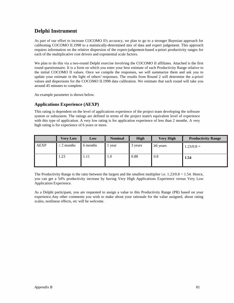
Appendix B 81
Delphi Instrument
As part of our effort to increase COCOMO II’s accuracy, we plan to go to a stronger Bayesian approach forcalibrating COCOMO II.1998 to a statistically-determined mix of data and expert judgement. This approachrequires information on the relative dispersion of the expert-judgement-based a-priori productivity ranges foreach of the multiplicative cost drivers and exponential scale factors.
We plan to do this via a two-round Delphi exercise involving the COCOMO II affiliates. Attached is the firstround questionnaire. It is a form on which you enter your best estimate of each Productivity Range relative tothe initial COCOMO II values. Once we compile the responses, we will summarize them and ask you toupdate your estimate in the light of others’ responses. The results from Round 2 will determine the a-priorivalues and dispersions for the COCOMO II.1998 data calibration. We estimate that each round will take youaround 45 minutes to complete.
An example parameter is shown below.
Applications Experience (AEXP)
This rating is dependent on the level of applications experience of the project team developing the softwaresystem or subsystem. The ratings are defined in terms of the project team’s equivalent level of experiencewith this type of application. A very low rating is for application experience of less than 2 months. A veryhigh rating is for experience of 6 years or more.
Very Low Low Nominal High Very High Productivity Range
AEXP ����PRQWKV 6 months 1 year 3 years ≥6 years 1.23/0.8 =
1.23 1.11 1.0 0.88 0.8 1.54
The Productivity Range is the ratio between the largest and the smallest multiplier i.e. 1.23/0.8 = 1.54. Hence,you can get a 54% productivity increase by having Very High Applications Experience versus Very LowApplication Experience.
As a Delphi participant, you are requested to assign a value to this Productivity Range (PR) based on yourexperience.Any other comments you wish to make about your rationale for the value assigned, about ratingscales, nonlinear effects, etc will be welcome.

Appendix B 82
Data Collection Instrument
Information on the Participant
Name :
Email address :
Phone Number :
Fax Number :
Snail Mail :
USC-CSE Point of Contact
For any questions or comments please contact :Sunita Devnani-ChulaniGraduate Research AssistantUSC -CSE [email protected]
Data Submission Address
Sunita Devnani-ChulaniCenter for Software EngineeringDepartment of Computer ScienceSalvatori 330University of Southern California941 W. 37th PlaceLos Angeles, CA 90089-0781

Appendix B 83
Cost DriversThese are the 17 effort multipliers used in COCOMO II Post-Architecture model to adjust the nominaleffort, Person Months, to reflect the software product under development. They are grouped into fourcategories: product, platform, personnel, and project.
Product Factors
Required Software Reliability (RELY)
This is the measure of the extent to which the software must perform its intended function over a period oftime. If the effect of a software failure is only slight inconvenience then RELY is low. If a failure would riskhuman life then RELY is very high.
Very Low Low Nominal High Very High Productivity Range(PR)
RELY slightinconvenience
low, easilyrecoverablelosses
moderate, easilyrecoverablelosses
high financialloss
risk tohuman life
1.4/0.75 =
0.75 0.88 1.0 1.15 1.4 1.87
Your PR value ______________
Data Base Size (DATA)
This measure attempts to capture the affect large data requirements have on productdevelopment. The rating is determined by calculating D/P. The reason the size of thedatabase is important to consider it because of the effort required to generate the test datathat will be used to exercise the program.
D
P
DataBaseSize Bytes
ogramSize SLOC=
( )
{Pr ( )
DATA is rated as low if D/P is less than 10 and it is very high if it is greater than 1000.
Low Nominal High Very High Productivity Range(PR)
DATA DB bytes/Pgm SLOC <10
10 �'�3������ 100 ��'�3��1000
D/P ������ 1.16/0.94 =
0.94 1.0 1.08 1.16 1.23
Your PR value ______________
Product Complexity (CPLX)
The table below provides the new COCOMO II CPLX rating scale. Complexity is divided into five areas:control operations, computational operations, device-dependent operations, data management operations,

Appendix B 84
and user interface management operations. Select the area or combination of areas that characterize theproduct or a sub-system of the product. The complexity rating is the subjective weighted average of theseareas.
Control OperationsComputational
OperationsDevice-dependent
OperationsData
ManagementOperations
User Interface ManagementOperations
Very Low
0.75
Straight-line code with a few non-nested structured programmingoperators: DOs, CASEs,IFTHENELSEs. Simple modulecomposition via procedure calls orsimple scripts.
Evaluation of simpleexpressions: e.g.,A=B+C*(D-E)
Simple read, writestatements with simpleformats.
Simple arraysin mainmemory.SimpleCOTS-DBqueries,updates.
Simple input forms, reportgenerators.
Low
0.88
Straightforward nesting of structuredprogramming operators. Mostly simplepredicates
Evaluation of moderate-level expressions: e.g.,D=SQRT(B**2-4.*A*C)
No cognizance needed ofparticular processor orI/O devicecharacteristics. I/O doneat GET/PUT level.
Single filesubsettingwith no datastructurechanges, noedits, nointermediate
Use of simple graphic userinterface (GUI) builders.
Nominal
1.0
Mostly simple nesting. Someintermodule control. Decision tables.Simple callbacks or message passing,including middleware-supporteddistributed processing
Use of standard math andstatistical routines. Basicmatrix/vector operations.
I/O processing includesdevice selection, statuschecking and errorprocessing.
Multi-fileinput andsingle fileoutput.Simplestructuralchanges
Simple use of widget set.
High
1.15
Highly nested structured programmingoperators with many compoundpredicates. Queue and stack control.Homogeneous, distributed processing.Single processor soft real-time control.
Basic numerical analysis:multivariate interpolation,ordinary differentialequations. Basictruncation, roundoffconcerns.
Operations at physicalI/O level (physicalstorage addresstranslations; seeks, reads,etc.). Optimized I/Ooverlap.
Simpletriggersactivated bydata streamcontents.Complex datarestructuring.
Widget set development andextension. Simple voice I/O,multimedia.
Very High
1.3
Reentrant and recursive coding. Fixed-priority interrupt handling. Tasksynchronization, complex callbacks,heterogeneous distributed processing.Single-processor hard real-timecontrol.
Difficult but structurednumerical analysis: near-singular matrix equations,partial differentialequations. Simpleparallelization.
Routines for interruptdiagnosis, servicing,masking.Communication linehandling. Performance-intensive embeddedsystems.
Distributeddatabasecoordination.Complextriggers.Searchoptimization.
Moderately complex 2D/3D,dynamic graphics, multimedia.
Extra High
1.65
Multiple resource scheduling withdynamically changing priorities.Microcode-level control. Distributedhard real-time control.
Difficult and unstructurednumerical analysis:highly accurate analysisof noisy, stochastic data.Complex parallelization.
Device timing-dependentcoding, micro-programmed operations.Performance-criticalembedded systems.
Highlycoupled,dynamicrelational andobjectstructures.Natural
Complex multimedia, virtualreality.
Productivity Range (PR) = 1.65/0.75 = 2.2 Your PR value ______________
Required Reusability (RUSE)
This cost driver accounts for the additional effort needed to construct components intended for reuse on thecurrent or future projects. This effort is consumed with creating more generic design of software, moreelaborate documentation, and more extensive testing to ensure components are ready for use in otherapplications.

Appendix B 85
Low Nominal High Very High Extra High Productivity Range
RUSE none acrossproject
acrossprogram
acrossproduct line
across multipleproduct lines
1.56/0.89 =
0.89 1.0 1.16 1.34 1.56 1.75
Your PR value _____________
Documentation match to life-cycle needs (DOCU)
Several software cost models have a cost driver for the level of required documentation. In COCOMO II,the rating scale for the DOCU cost driver is evaluated in terms of the suitability of the project’sdocumentation to its life-cycle needs. The rating scale goes from Very Low (many life-cycle needsuncovered) to Very High (very excessive for life-cycle needs).
Very Low Low Nominal High Very High Productivity Range
DOCU Many life-cycle needsuncovered
Some life-cycle needsuncovered
Right-sizedto life-cycleneeds
Excessive forlife-cycleneeds
Very excessivefor life-cycleneeds
1.17/0.85 =
0.85 0.93 1.0 1.08 1.17 1.38
Your PR value______________

Appendix B 86
Platform FactorsThe platform refers to the target-machine complex of hardware and infrastructure software (previouslycalled the virtual machine). The factors have been revised to reflect this as described in this section. Someadditional platform factors were considered, such as distribution, parallelism, embeddedness, and real-timeoperations.
Execution Time Constraint (TIME)
This is a measure of the execution time constraint imposed upon a software system. The rating is expressedin terms of the percentage of available execution time expected to be used by the system or subsystemconsuming the execution time resource. The rating ranges from nominal, less than 50% of the executiontime resource used, to extra high, 95% of the execution time resource is consumed.
Nominal High Very High Extra High Productivity Range (PR)
TIME Û 50% use of availableexecution time
70% 85% 95% 1.66/1.0 =
1.0 1.11 1.3 1.66 1.66
Your PR value______________
Main Storage Constraint (STOR)
This rating represents the degree of main storage constraint imposed on a software system or subsystem.Given the remarkable increase in available processor execution time and main storage, one can questionwhether these constraint variables are still relevant. However, many applications continue to expand toconsume whatever resources are available, making these cost drivers still relevant. The rating ranges fromnominal, less that 50%, to extra high, 95%.
Nominal High Very High Extra High Productivity Range (PR)
STOR �����XVH�RIavailable storage
70% 85% 95% 1.56/1.0 =
1.0 1.06 1.21 1.56 1.56
Your PR value______________

Appendix B 87
Platform Volatility (PVOL)
"Platform" is used here to mean the complex of hardware and software (OS, DBMS, etc.) the softwareproduct calls on to perform its tasks. If the software to be developed is an operating system then theplatform is the computer hardware. If a database management system is to be developed then the platform isthe hardware and the operating system. If a network text browser is to be developed then the platform is thenetwork, computer hardware, the operating system, and the distributed information repositories. Theplatform includes any compilers or assemblers supporting the development of the software system. Thisrating ranges from low, where there is a major change every 12 months, to very high, where there is a majorchange every two weeks.
Low Nominal High Very High Productivity Range (PR)
PVOL major change every 12mo.; minor change every1 mo.
major: 6 mo.;minor: 2 wk.
major: 2 mo.;minor: 1 wk.
major: 2 wk.;minor: 2 days
1.3/0.87 =
0.87 1.0 1.15 1.30 1.49
Your PR value______________

Appendix B 88
Personnel Factors
Analyst Capability (ACAP)
Analysts are personnel that work on requirements, high level design and detailed design. The majorattributes that should be considered in this rating are Analysis and Design ability, efficiency andthoroughness, and the ability to communicate and cooperate. The rating should not consider the level ofexperience of the analyst; that is rated with AEXP. Analysts that fall in the 15th percentile are rated verylow and those that fall in the 95th percentile are rated as very high..
Very Low Low Nominal High Very High Productivity Range(PR)
ACAP 15thpercentile
35thpercentile
55thpercentile
75thpercentile
90th percentile 1.5/0.67 =
1.5 1.22 1.0 0.83 0.67 2.24
Your PR value______________
Programmer Capability (PCAP)
Current trends continue to emphasize the importance of highly capable analysts. However the increasingrole of complex COTS packages, and the significant productivity leverage associated with programmers’ability to deal with these COTS packages, indicates a trend toward higher importance of programmercapability as well.
Evaluation should be based on the capability of the programmers as a team rather than as individuals. Majorfactors which should be considered in the rating are ability, efficiency and thoroughness, and the ability tocommunicate and cooperate. The experience of the programmer should not be considered here; it is ratedwith AEXP. A very low rated programmer team is in the 15th percentile and a very high rated programmerteam is in the 95th percentile.
Very Low Low Nominal High Very High Productivity Range (PR)
PCAP 15thpercentile
35thpercentile
55thpercentile
75thpercentile
90th percentile 1.37/0.74 =
1.37 1.16 1.0 0.87 0.74 1.85
Your PR value______________
Applications Experience (AEXP)
This rating is dependent on the level of applications experience of the project team developing the softwaresystem or subsystem. The ratings are defined in terms of the project team’s equivalent level of experiencewith this type of application. A very low rating is for application experience of less than 2 months. A veryhigh rating is for experience of 6 years or more..

Appendix B 89
Very Low Low Nominal High Very High Productivity Range (PR)
AEXP ����PRQWKV 6 months 1 year 3 years 6 years 1.23/0.8 =
1.23 1.1 1.0 0.88 0.8 1.54
Your PR value______________
Platform Experience (PEXP)
The Post-Architecture model broadens the productivity influence of PEXP, recognizing the importance ofunderstanding the use of more powerful platforms, including more graphic user interface, database,networking, and distributed middleware capabilities.
Very Low Low Nominal High Very High Productivity Range (PR)
PEXP ����PRQWKV 6 months 1 year 3 years 6 year 1.26/0.8 =
1.26 1.12 1.0 0.88 0.8 1.58
Your PR value______________
Language and Tool Experience (LTEX)
This is a measure of the level of programming language and software tool experience of the project teamdeveloping the software system or subsystem. Software development includes the use of tools that performrequirements and design representation and analysis, configuration management, document extraction,library management, program style and formatting, consistency checking, etc. In addition to experience inprogramming with a specific language the supporting tool set also effects development time. A low ratinggiven for experience of less than 2 months. A very high rating is given for experience of 6 or more years.
Very Low Low Nominal High Very High Productivity Range (PR)
LTEX ����PRQWKV 6 months 1 year 3 years 6 year 1.24/0.82 =
1.24 1.11 1.0 0.9 0.82 1.51
Your PR value______________
Personnel Continuity (PCON)
The rating scale for PCON is in terms of the project’s annual personnel turnover: from 3%, very high, to48%, very low.
Very Low Low Nominal High Very High Productivity Range(PR)
PCON 48% / year 24% / year 12% / year 6% / year 3% / year 1.26/0.83 =
1.26 1.11 1.0 0.91 0.83 1.52
Your PR value______________

Appendix B 90
Project Factors
Use of Software Tools (TOOL)
Software tools have improved significantly since the 1970’s projects used to calibrate COCOMO. The toolrating ranges from simple edit and code, very low, to integrated lifecycle management tools, very high.
Very Low Low Nominal High Very High ProductivityRange (PR)
TOOL edit, code,debug
simple,frontend,backendCASE, littleintegration
basic lifecycletools,moderatelyintegrated
strong, maturelifecycle tools,moderatelyintegrated
strong, mature,proactive lifecycletools, wellintegrated withprocesses,methods, reuse
1.2/0.75 =
1.2 1.1 1.0 0.88 0.75 1.6
Your PR value______________
Multisite Development (SITE)
Given the increasing frequency of multisite developments, and indications that multisite developmenteffects are significant, the SITE cost driver has been added in COCOMO II. Determining its cost driverrating involves the assessment and averaging of two factors: site collocation (from fully collocated tointernational distribution) and communication support (from surface mail and some phone access to fullinteractive multimedia).
VeryLow
Low Nominal High Very High Extra High ProductivityRange (PR)
SITE:Commu-nications
SITE:
Collocation
Somephone,mail
International
Indivi-dualphone,FAX
Multicityand -Multicompany
Narrow-band email
MulticityorMulticompany
Wide-bandelectroniccommuni-cation.
Same city ormetro area
Widebandelect.comm,occasionalvideoconf.
Samebuilding
Inter activemulti media
Fullycollocated
1.24/0.79 =
1.24 1.1 1.0 0.92 0.85 0.79 1.57
Your PR value_____________

Appendix B 91
Required Development Schedule (SCED)
This rating measures the schedule constraint imposed on the project team developing the software. Theratings are defined in terms of the percentage of schedule stretch-out or acceleration with respect to anominal schedule for a project requiring a given amount of effort. Accelerated schedules tend to producemore effort in the later phases of development because more issues are left to be determined due to lack oftime to resolve them earlier. A schedule compress of 74% is rated very low. A stretch-out of a scheduleproduces more effort in the earlier phases of development where there is more time for thorough planning,specification and validation. A stretch-out of 160% is rated very high.
Very Low Low Nominal High Very High Productivity Range (PR)
SCED 75% of nominal 85% 100% 130% 160% 1.23/1.0 =
1.23 1.08 1.0 1.0 1.0 1.23
Your PR value______________

Appendix B 92
Scale FactorsSoftware cost estimation models often have an exponential factor to account for the relative economies ordiseconomies of scale encountered in different size software projects. The exponent, B, in Equation 1 isused to capture these effects.
If B < 1.0, the project exhibits economies of scale. If the product’s size is doubled, the project effort is lessthan doubled. The project’s productivity increases as the product size is increased. Some project economiesof scale can be achieved via project-specific tools (e.g., simulations, testbeds) but in general these aredifficult to achieve. For small projects, fixed start-up costs such as tool tailoring and setup of standards andadministrative reports are often a source of economies of scale.
If B = 1.0, the economies and diseconomies of scale are in balance. This linear model is often used for costestimation of small projects. It is used for the COCOMO II Applications Composition model.
If B > 1.0, the project exhibits diseconomies of scale. This is generally due to two main factors: growth ofinterpersonal communications overhead and growth of large-system integration overhead. Larger projectswill have more personnel, and thus more interpersonal communications paths consuming overhead.Integrating a small product as part of a larger product requires not only the effort to develop the smallproduct, but also the additional overhead effort to design, maintain, integrate, and test its interfaces with theremainder of the product.
The data analysis on the original COCOMO indicated that its projects exhibited net diseconomies of scale.The projects factored into three classes or modes of software development (Organic, Semidetached, andEmbedded), whose exponents B were 1.05, 1.12, and 1.20, respectively. The distinguishing factors of thesemodes were basically environmental: Embedded-mode projects were more unprecedented, requiring morecommunication overhead and complex integration; and less flexible, requiring more communicationsoverhead and extra effort to resolve issues within tight schedule, budget, interface, and performanceconstraints.
The scaling model in Ada COCOMO continued to exhibit diseconomies of scale, but recognized that agood deal of the diseconomy could be reduced via management controllables. Communications overheadand integration overhead could be reduced significantly by early risk and error elimination; by usingthorough, validated architectural specifications; and by stabilizing requirements. These practices werecombined into an Ada process model [Boehm and Royce 1989, Royce 1990]. The project’s use of thesepractices, and an Ada process model experience or maturity factor, were used in Ada COCOMO todetermine the scale factor B.
Ada COCOMO applied this approach to only one of the COCOMO development modes, the Embeddedmode. Rather than a single exponent B = 1.20 for this mode, Ada COCOMO enabled B to vary from 1.04 to1.24, depending on the project’s progress in reducing diseconomies of scale via early risk elimination, solidarchitecture, stable requirements, and Ada process maturity.
COCOMO II combines the COCOMO and Ada COCOMO scaling approaches into a single rating-drivenmodel. It is similar to that of Ada COCOMO in having additive factors applied to a base exponent B. Itincludes the Ada COCOMO factors, but combines the architecture and risk factors into a single factor, andreplaces the Ada process maturity factor with a Software Engineering Institute (SEI) process maturity factor(The exact form of this factor is still being worked out with the SEI). The scaling model also adds twofactors, precedentedness and flexibility, to account for the mode effects in original COCOMO, and adds aTeam Cohesiveness factor to account for the diseconomy-of-scale effects on software projects whosedevelopers, customers, and users have difficulty in synchronizing their efforts. It does not include the AdaCOCOMO Requirements Volatility factor, which is now covered by increasing the effective product sizevia the Breakage factor.
Equation 1 defines the exponent, B. The table below provides the rating levels for the COCOMO II scaledrivers. The selection of scale drivers is based on the rationale that they are a significant source ofexponential variation on a project’s effort or productivity variation. Each scale driver has a range of ratinglevels, from Very Low to Extra High. Each rating level has a weight, W, and the specific value of the weight

Appendix B 93
is called a scale factor. A project’s scale factors, Wi, are summed across all of the factors, and used todetermine a scale exponent, B, via the following formula:
B Wi= + × ∑101 0 01. . EQ 1.
For example, if scale factors with an Extra High rating are each assigned a weight of (0), then a 100KSLOC project with Extra High ratings for all factors will have ∑Wi = 0, B = 1.01, and a relative effort E= 1001.01= 105 PM. If scale factors with Very Low rating are each assigned a weight of (5), then a projectwith Very Low (5) ratings for all factors will have ∑Wi = 25, B = 1.26, and a relative effort E = 331 PM.This represents a large variation, but the increase involved in a one-unit change in one of the factors is onlyabout 4.7%.
The Productivity Range (PR) for a 100KSLOC project is computed as (100)1.06 / (100) 1.01 = 131.83 / 104.71= 1.26
For all the five Scale Factors we will use a 100 KSLOC project as the baseline project.
ScaleFactors
(Wi)
Very Low Low Nominal High Very High Extra High PR
PREC thoroughlyunprecedented
largelyunprecedented
somewhatunprecedented
generallyfamiliar
largelyfamiliar
thoroughlyfamiliar
(100)1.06 /(100) 1.01=
5 4 3 2 1 0 1.26
Your PR value______________
ScaleFactors
(Wi)
Very Low Low Nominal High Very High Extra High PR
FLEX rigorous occasionalrelaxation
some
relaxation
general
conformity
some
conformity
general goals (100)1.06 /(100) 1.01=
5 4 3 2 1 0 1.26
Your PR value______________
ScaleFactors
(Wi)
Very Low Low Nominal High Very High Extra High PR
RESLa little (20%) some (40%) often (60%) generally(75%)
mostly(90%)
full (100%) (100)1.06 /(100) 1.01=
5 4 3 2 1 0 1.26
a % significant module interfaces specified, % significant risks eliminated.
Your PR value______________

Appendix B 94
ScaleFactors
(Wi)
Very Low Low Nominal High Very High Extra High PR
TEAM verydifficultinteractions
somedifficultinteractions
basicallycooperativeinteractions
largely
cooperative
highly
cooperative
seamlessinteractions
(100)1.06/(100) 1.01
=
5 4 3 2 1 0 1.26
Your PR value______________
ScaleFactors
(Wi)
Very Low Low Nominal High Very High Extra High PR
PMAT Weighted average of "Yes" answers to CMM Maturity Questionnaire (100)1.06 /(100) 1.01=
5 4 3 2 1 0 1.26
Your PR value______________

Appendix B 95

Appendix C 97
Appendix C: Defect Introduction Model Behavioral Analysis and Results of Two-Round Delphi
PERSONNEL FACTORS
Analyst Capability (ACAP)
ACAPlevel
Requirements Design Code
VH Fewer Requirementsunderstanding defectsFewer RequirementsCompleteness, consistencydefects
0.75
Fewer Requirements traceabilitydefectsFewer Design Completeness,consistency defectsFewer defects introduced in fixingdefects
0.83
Fewer Coding defects due torequirements, designshortfalls-missing guidelines-ambiguities
0.90Nominal Nominal level of defect introduction
1.0VL More Requirements
understanding defectsMore RequirementsCompleteness, consistencydefects
1.33
More Requirements traceabilitydefectsMore Design Completeness,consistency defectsMore defects introduced in fixingdefects
1.20
More Coding defects due torequirements, designshortfalls-missing guidelines-ambiguities
1.11Initial Quality Range 1.77 1.45 1.23Range - Round 1 1.4-2 1.3-1.8 1-1.4Median - Round 1 1.92 1.48 1.23Range - Round 2 1.7-2 1.4-1.69 1.2-1.41Final Quality Range(Median - Round 2)
1.77 1.45 1.23
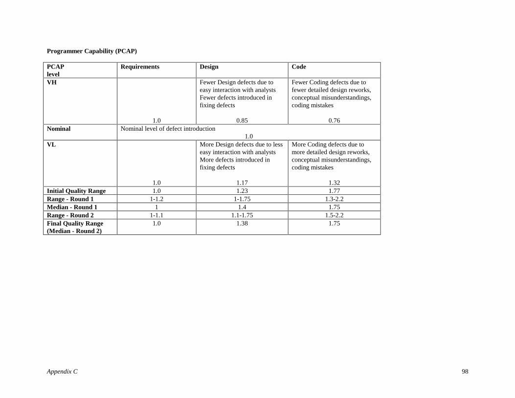
Appendix C 98
Programmer Capability (PCAP)
PCAPlevel
Requirements Design Code
VH
1.0
Fewer Design defects due toeasy interaction with analystsFewer defects introduced infixing defects
0.85
Fewer Coding defects due tofewer detailed design reworks,conceptual misunderstandings,coding mistakes
0.76Nominal Nominal level of defect introduction
1.0VL
1.0
More Design defects due to lesseasy interaction with analystsMore defects introduced infixing defects
1.17
More Coding defects due tomore detailed design reworks,conceptual misunderstandings,coding mistakes
1.32Initial Quality Range 1.0 1.23 1.77Range - Round 1 1-1.2 1-1.75 1.3-2.2Median - Round 1 1 1.4 1.75Range - Round 2 1-1.1 1.1-1.75 1.5-2.2Final Quality Range(Median - Round 2)
1.0 1.38 1.75

Appendix C 99
Applications Experience (AEXP)
AEXP level Requirements Design CodeVH Fewer Requirements defects due
to less learning and fewer falsestartsFewer Requirementsunderstanding defects
0.81
Fewer Design defects due to lesslearning and fewer false startsFewer Requirements traceabilitydefectsFewer defects introduced infixing requirements, preliminarydesign fixes
0.82
Fewer Coding defects due toless learningFewer Coding defects due torequirements, designshortfalls
0.88Nominal Nominal level of defect introduction
1.0VL More Requirements defects due
to extensive learning and morefalse startsMore Requirementsunderstanding defects
1.24
More Design defects due to lesslearning and fewer false startsMore Requirements traceabilitydefectsMore defects introduced infixing requirements, preliminarydesign fixes
1.22
More Coding defects due toextensive learningMore Coding defects due torequirements, designshortfalls
1.13Initial Quality Range 1.56 1.56 1.32Range - Round 1 1.4-1.65 1.3-1.56 1.05-1.4Median - Round 1 1.5 1.5 1.26Range - Round 2 1.5-1.6 1.4-1.56 1.2-1.32Final Quality Range(Median - Round 2)
1.53 1.5 1.28

Appendix C 100
Platform Experience (PEXP)
PEXP level Requirements Design CodeVH Fewer Requirements defects due
to fewer application/platform∗
interface analysismisunderstandings
0.90
Fewer Design defects due tofewer application/platforminterface designmisunderstandings
0.86
Fewer Coding defects due toapplication/platforminterface codingmisunderstandings
0.86Nominal Nominal level of defect introduction
1.0VL More Requirements defects due to
more application/platform*
interface, database, networkinganalysis misunderstandings
1.11
More Design defects due tomore application/platforminterface designmisunderstandings
1.17
More Coding defects due toapplication/platforminterface codingmisunderstandings
1.16Initial Quality Range 1.23 1.32 1.32Range - Round 1 1.1-1.3 1.2-1.45 1.28-1.5Median - Round 1 1.2 1.4 1.4Range - Round 2 1.1-1.3 1.3-1.4 1.3-1.5Final Quality Range(Median - Round 2)
1.23 1.36 1.35
∗ “Platform” can include office automation, database, and user-interface support packages; distributed middleware; operating systems; networking support; andhardware.
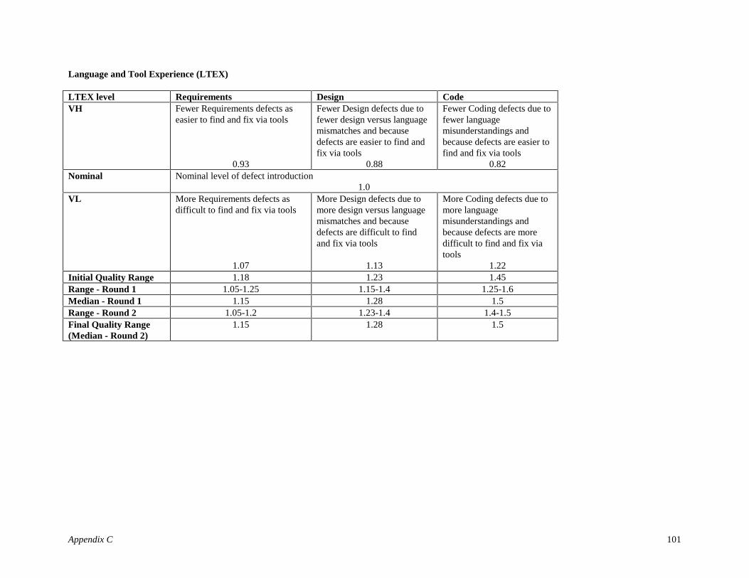
Appendix C 101
Language and Tool Experience (LTEX)
LTEX level Requirements Design CodeVH Fewer Requirements defects as
easier to find and fix via tools
0.93
Fewer Design defects due tofewer design versus languagemismatches and becausedefects are easier to find andfix via tools
0.88
Fewer Coding defects due tofewer languagemisunderstandings andbecause defects are easier tofind and fix via tools
0.82Nominal Nominal level of defect introduction
1.0VL More Requirements defects as
difficult to find and fix via tools
1.07
More Design defects due tomore design versus languagemismatches and becausedefects are difficult to findand fix via tools
1.13
More Coding defects due tomore languagemisunderstandings andbecause defects are moredifficult to find and fix viatools
1.22Initial Quality Range 1.18 1.23 1.45Range - Round 1 1.05-1.25 1.15-1.4 1.25-1.6Median - Round 1 1.15 1.28 1.5Range - Round 2 1.05-1.2 1.23-1.4 1.4-1.5Final Quality Range(Median - Round 2)
1.15 1.28 1.5

Appendix C 102
Personnel Continuity (PCON)
PCON level Requirements Design CodeVH Fewer Requirements
understanding defectsFewer Requirementscompleteness, consistency defects.Fewer Requirements defects dueto false starts
0.82
Fewer Requirementstraceability defectsFewer Design completeness,consistency defectsFewer defects introduced infixing defects
0.80
Fewer Coding defects due torequirements, designshortfalls, misunderstandings-missing guidelines, context-ambiguitiesFewer defects introduced infixing defects
0.77Nominal Nominal level of defect introduction
1.0VL More Requirements understanding
defectsMore Requirements completeness,consistency defects.More Requirements defects due tofalse starts
1.22
More Requirementstraceability defectsMore Design completeness,consistency defectsMore defects introduced infixing defects
1.25
More Coding defects due torequirements, designshortfalls, misunderstandings-missing guidelines, context-ambiguitiesMore defects introduced infixing defects
1.30Initial Quality Range 1.45 1.56 1.77Range - Round 1 1.1-2 1.1-2 1.1-2Median - Round 1 1.5 1.58 1.65Range - Round 2 1.45-2 1.5-2 1.4-2Final Quality Range(Median - Round 2)
1.5 1.57 1.69

Appendix C 103
PROJECT FACTORS
Use of Software Tools (TOOL)
TOOL level Requirements Design CodeVH Fewer Requirements defects as
easier to find and fix via tools
0.92
Fewer Design defects aseasier to fix and find via tools
0.91
Fewer Coding defects aseasier to find and fix viatoolsFewer defects due toautomation of translation ofdetailed design into code
0.80Nominal Nominal level of defect introduction
1.0VL More Requirements defects as
harder to find and fix via tools
1.09
More Design defects as harderto find and fix via tools
1.10
More Coding defects asharder to find and fix viatoolsMore defects due to manualtranslation of detailed designinto code
1.25Initial Quality Range 1.18 1.18 1.56Range - Round 1 0.98-1.4 1.02-1.4 1.1-1.8Median - Round 1 1.15 1.25 1.6Range - Round 2 1.1-1.3 1.1-1.3 1.45-1.7Final Quality Range(Median - Round 2)
1.18 1.2 1.56

Appendix C 104
Multisite Development (SITE)
SITE level Requirements Design CodeXH Fewer Requirements
understanding, completeness andconsistency defects due to sharedcontext, good communicationsupport
0.83
Fewer Requirementstraceability defects, Designcompleteness, consistencydefects due to shared context,good communication supportFewer defects introduced infixing defects
0.83
Fewer Coding defects due torequirements, designshortfalls andmisunderstandings; sharedcoding contextFewer defects introduced infixing defects
0.85Nominal Nominal level of defect introduction
1.0VL More Requirements
understanding, completeness andconsistency defects due to lack ofshared context, poorcommunication support
1.20
More Requirementstraceability defects, Designcompleteness, consistencydefects due to lack of sharedcontext, poor communicationsupportMore defects introduced infixing defects
1.20
More Coding defects due torequirements, designshortfalls andmisunderstandings; lack ofshared contextMore defects introduced infixing defects
1.18Initial Quality Range 1.45 1.45 1.45Range - Round 1 1.2-1.65 1.2-1.6 1.1-1.5Median - Round 1 1.4 1.5 1.4Range - Round 2 1.3-1.5 1.2-1.5 1.2-1.5Final Quality Range(Median - Round 2)
1.45 1.45 1.4

Appendix C 105
Required Development Schedule (SCED)
SCED level Requirements Design CodeVH Fewer requirements defects due to
higher likelihood of correctlyinterpreting specsFewer defects due to morethorough planning, specs,validation
0.85
Fewer Design defects due tohigher likelihood of correctlyinterpreting specsFewer Design defects due tofewer defects in fixes andfewer specification defects tofixFewer defects due to morethorough planning, specs,validation
0.84
Fewer Coding defects due tohigher likelihood ofcorrectly interpreting specsFewer Coding defects due torequirements and designshortfallsFewer defects introduced infixing defects
0.84Nominal Nominal level of defect introduction
1.0VL More Requirements defects due to
- more interface problems (morepeople in parallel) - more TBDs in specs, plans - less time for validation
1.18
More Design defects due toearlier TBDs, more interfaceproblems, less time for V&VMore defects in fixes andmore specification defects tofix
1.19
More Coding defects due torequirements and designshortfalls, less time for V&VMore defects introduced infixing defects
1.19Initial Quality Range 1.39 1.41 1.41Range - Round 1 1.2-2 1.25-1.7 1.2-2.1Median - Round 1 1.45 1.45 1.58Range - Round 2 1.3-1.8 1.4-1.7 1.3-1.9Final Quality Range(Median - Round 2)
1.4 1.42 1.42

Appendix C 106
PLATFORM FACTORS
Execution Time Constraint (TIME)
TIME level Requirements Design CodeXH More Requirements Defects due
to trickier analysis, complexinterface design, test plans andmore planning
1.08
More Design Defects due totrickier analysis, complexinterface design, test plans andmore planning
1.2
More Coding Defects sincecode and data trickier todebug
1.2Nominal Nominal or lower level of defect introduction
1.0Initial Quality Range 1.08 1.15 1.15Range - Round 1 1-2 1.1-2 1.1-2Median - Round 1 1.07 1.2 1.21Range - Round 2 1.08-1.1 1.15-1.25 1.15-1.25Final Quality Range(Median - Round 2)
1.08 1.2 1.2

Appendix C 107
Main Storage Constraint (STOR)
STOR level Requirements Design CodeXH More Requirements
understanding defects due totrickier analysis
1.08
More Design defects due totrickier analysis
1.18
More Coding defects sincecode and data trickier todebug
1.15Nominal Nominal or lower level of defect introduction
1.0Initial Quality Range 1.08 1.15 1.15Range - Round 1 1-2 1.1-2 1.1-2Median - Round 1 1.05 1.2 1.2Range - Round 2 1.05-1.1 1.1-1.2 1.1-1.2Final Quality Range(Median - Round 2)
1.08 1.18 1.15
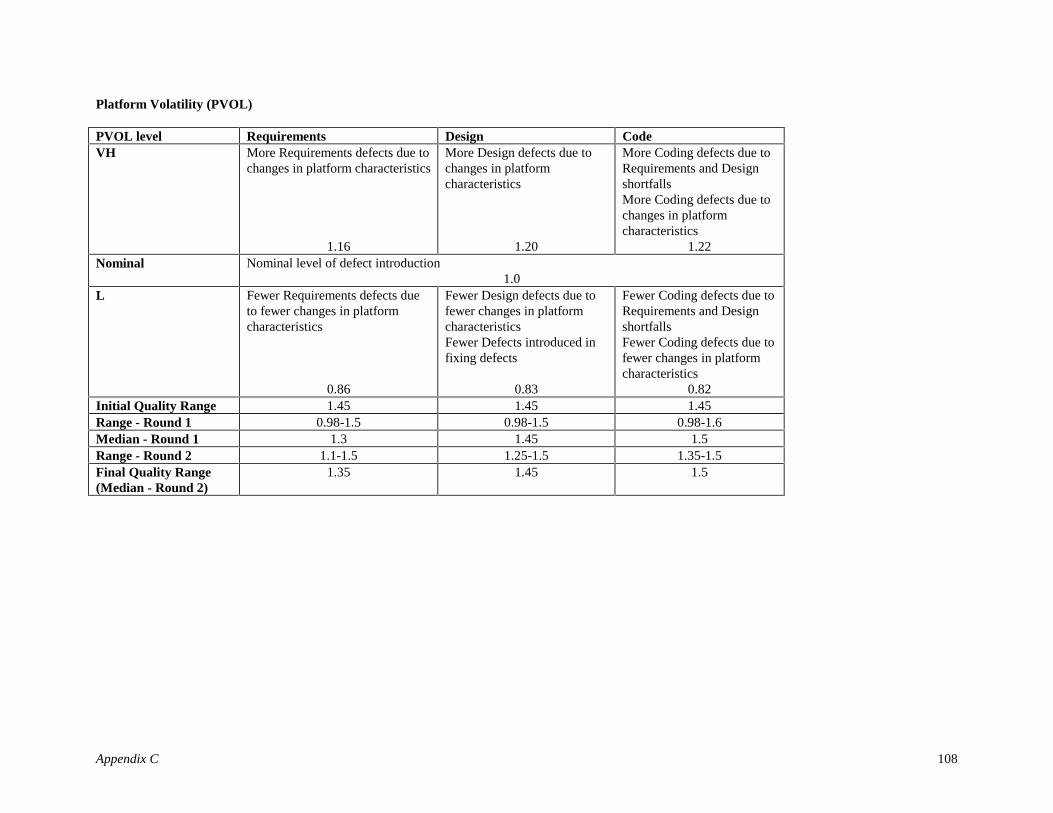
Appendix C 108
Platform Volatility (PVOL)
PVOL level Requirements Design CodeVH More Requirements defects due to
changes in platform characteristics
1.16
More Design defects due tochanges in platformcharacteristics
1.20
More Coding defects due toRequirements and DesignshortfallsMore Coding defects due tochanges in platformcharacteristics
1.22Nominal Nominal level of defect introduction
1.0L Fewer Requirements defects due
to fewer changes in platformcharacteristics
0.86
Fewer Design defects due tofewer changes in platformcharacteristicsFewer Defects introduced infixing defects
0.83
Fewer Coding defects due toRequirements and DesignshortfallsFewer Coding defects due tofewer changes in platformcharacteristics
0.82Initial Quality Range 1.45 1.45 1.45Range - Round 1 0.98-1.5 0.98-1.5 0.98-1.6Median - Round 1 1.3 1.45 1.5Range - Round 2 1.1-1.5 1.25-1.5 1.35-1.5Final Quality Range(Median - Round 2)
1.35 1.45 1.5

Appendix C 109
PRODUCT FACTORS
Required Software Reliability (RELY)
RELY level Requirements Design CodeVH Fewer Requirements
Completeness, consistency defectsdue to detailed verification, QA,CM, standards, SSR,documentation, IV&V interface,test plans, procedures
0.70
Fewer Design defects due todetailed verification, QA,CM, standards, PDR,documentation, IV&Vinterface, design inspections,test plans, procedures
0.69
Fewer Coding defects due todetailed verification, QA,CM, standards,documentation, IV&Vinterface, code inspections,test plans, procedures
0.69Nominal Nominal level of defect introduction
1.0VL More Requirements
Completeness, consistency defectsdue to minimal verification, QA,CM, standards, PDR,documentation, IV&V interface,test plans, procedures
1.43
More Design defects due tominimal verification, QA,CM, standards, PDR,documentation, IV&Vinterface, design inspections,test plans, procedures
1.45
More Coding defects due tominimal verification, QA,CM, standards, PDR,documentation, IV&Vinterface, code inspections,test plans, procedures
1.45Initial Quality Range 2.24 2.24 2.24Range - Round 1 1.2-2.61 1.2-2.61 1.2-2.61Median - Round 1 2 2 2Range - Round 2 1.8-2.24 1.9-2.3 2-2.24Final Quality Range(Median - Round 2)(Median - Round 2)
2.05 2.1 2.1

Appendix C 110
Data Base Size (DATA)
DATA level Requirements Design CodeVH More Requirements defects due to
- complex database design andvalidation - complex HW/SW storageinterface
1.07
More Design defects due to - complex database designand validation - complex HW/SW storageinterface - more data checking inprogram
1.10
More Coding defects due to - complex databasedevelopment - complex HW/SW storageinterface - more data checking inprogram
1.10Nominal Nominal level of defect introduction
1.0L Fewer Requirements defects due
to - simple database design andvalidation - simple HW/SW storageinterface
0.93
Fewer Design defects due to - simple database design andvalidation - simple HW/SW storageinterface - simple data checking inprogram
0.91
Fewer Coding defects due to - simple databasedevelopment - Simple HW/SW storageinterface - simple data checking inprogram
0.91Initial Quality Range 1.15 1.22 1.22Range - Round 1 1-1.15 1-1.35 1-1.3Median - Round 1 1.12 1.23 1.23Range - Round 2 1.1-1.15 1.2-1.3 1.2-1.3Final Quality Range(Median - Round 2)
1.15 1.21 1.21

Appendix C 111
Required Reusability (RUSE)
RUSE level Requirements Design CodeXH More Requirements defects due to
higher complexity in design,validation and interfaces.Fewer Requirements defects dueto more thorough interfaceanalysis
1.05
More Design defects due tohigher complexity in design,validation and interfacesFewer Requirements defectsdue to more thorough interfaceanalysis
1.02
More Coding defects due tohigher complexity in design,validation and interfacesFewer Requirements defectsdue to more thoroughinterface definitions
1.02Nominal Nominal level of defect introduction
1.0L Fewer Requirements Defects due
to lower complexity in design,validation and interfaces.
0.95
Fewer Design defects due tolower complexity in design,validation, test plans andinterfaces
0.98
Fewer Coding defects due tolower complexity in design,validation, test plans andinterfaces
0.98Initial Quality Range 1.02 1.04 1.04Range - Round 1 1-1.5 1-2.5 1-3Median - Round 1 1.1 1.1 1.05Range - Round 2 1-1.5 1-2 1-2.5Final Quality Range(Median - Round 2)
1.1 1.05 1.05
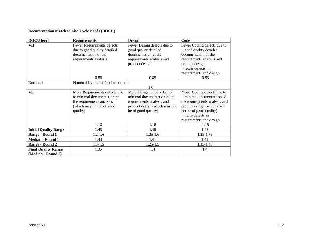
Appendix C 112
Documentation Match to Life-Cycle Needs (DOCU)
DOCU level Requirements Design CodeVH Fewer Requirements defects
due to good quality detaileddocumentation of therequirements analysis
0.86
Fewer Design defects due togood quality detaileddocumentation of therequirements analysis andproduct design
0.85
Fewer Coding defects due to - good quality detaileddocumentation of therequirements analysis andproduct design - fewer defects inrequirements and design
0.85Nominal Nominal level of defect introduction
1.0VL More Requirements defects due
to minimal documentation ofthe requirements analysis(which may not be of goodquality)
1.16
More Design defects due tominimal documentation of therequirements analysis andproduct design (which may notbe of good quality)
1.18
More Coding defects due to - minimal documentation ofthe requirements analysis andproduct design (which maynot be of good quality) - more defects inrequirements and design
1.18Initial Quality Range 1.45 1.45 1.45Range - Round 1 1.2-1.6 1.25-1.6 1.25-1.75Median - Round 1 1.43 1.41 1.41Range - Round 2 1.3-1.5 1.25-1.5 1.35-1.45Final Quality Range(Median - Round 2)
1.35 1.4 1.4

Appendix C 113
Product Complexity (CPLX)
CPLX level Requirements Design CodeXH More Requirements
understanding defectsMore Requirements Defects dueto - complex specification andvalidation - complex interfaces
1.32
More Design defects due to - complex design andvalidation - complex interfaces
1.41
More Coding defects due to - complex data and controlstructures - complex interfacesMore Coding defects due toRequirements and Designshortfalls
1.41Nominal Nominal level of defect introduction
1.0VL Fewer Requirements
understanding defectsFewer Requirements Defects dueto- simpler specification andvalidation- simpler interfaces
0.76
Fewer Design defects due to - simpler design andvalidation - simpler interfaces
0.71
Fewer Coding defects due to - simpler data and controlstructures - simpler interfacesFewer Coding defects due toRequirements and Designshortfalls
0.71Initial Quality Range 1.75 2.00 2.00Range - Round 1 1.5-2 1.8-2.25 1.7-2Median - Round 1 1.89 2 1.9Range - Round 2 1.7-1.8 1.8-2.1 1.9-2Final Quality Range(Median - Round 2)
1.74 2.0 2.0

Appendix C 114
Disciplined Methods (DISC)* - e.g. Cleanroom, PSP
DISC level Requirements Design CodeVH Fewer Requirements defects due
to- more thorough specs- more emphasis on defectprevention
0.63
Fewer Design defects dueto- more thorough specs- more emphasis on defectprevention
0.60
Fewer Coding defects due to- extensive self-review- more emphasis on defectprevention- extensive defect checklists- defensive programming- independent unit testing
0.54Nominal Nominal level of defect introduction
1.0VL More Requirements defects due to
- less thorough specs- less emphasis on defectprevention
1.58
More Design defects dueto- less thorough specs- less emphasis on defectprevention
1.67
More Coding defects due to- minimal self-review- less emphasis on defectprevention- minimal defect checklists- lack of defensiveprogramming- lack of independent unittesting
1.84Initial Quality Range 2.24 2.78 4.00Range - Round 1 1.75-10 2-10 2.5-10Median - Round 1 2.5 2.91 3Range - Round 2 1.75-3 2-3 3-4Final Quality Range(Median - Round 2)
2.5 2.78 3.4
* This Defect Driver is in addition to the 22 COCOMO II drivers

Appendix C 115
Precedentedness (PREC)
PREC level Requirements Design CodeXH Fewer Requirements
defects due to lesslearning and fewer falsestartsFewer Requirementsunderstanding defectsFewer Requirementsdefects since very littleconcurrent developmentof associated newhardware or operationalprocedures
0.70 (VH = 0.84)
Fewer Design defects due to lesslearning and fewer false startsFewer Requirements traceabilitydefectsFewer Design defects since very littleconcurrent development of associatednew hardware or operationalproceduresFewer Design defects since minimalneed for innovative data processingarchitectures, algorithmsFewer defects introduced in fixingrequirements, preliminary design fixes
0.75 (VH = 0.87)
Fewer Coding defects due to lesslearningFewer Coding defects due torequirements, design shortfallsFewer Coding defects since verylittle concurrent development ofassociated new hardware oroperational proceduresFewer Coding defects sinceminimal need for innovative dataprocessing architectures,algorithms
0.81 (VH = 0.90)Nominal Nominal level of defect introduction
1.0VL More Requirements
defects due to morelearning and more falsestartsMore Requirementsunderstanding defectsMore Requirementsdefects since extensiveconcurrent developmentof associated newhardware or operationalprocedures
1.43
More Design defects due to morelearning and more false startsMore Requirements traceability defectsMore Design defects since extensiveconcurrent development of associatednew hardware or operationalproceduresMore Design defects since considerableneed for innovative data processingarchitectures, algorithmsMore defects introduced in fixingrequirements, preliminary design fixes
1.34
More Coding defects due to morelearningMore Coding defects due torequirements, design shortfallsMore Coding defects sinceextensive concurrent developmentof associated new hardware oroperational proceduresMore Coding defects sinceconsiderable need for innovativedata processing architectures,algorithms
1.24Initial Quality Range 2.05 1.74 1.58Range - Round 1 1.7-2.5 1.6-2 1.4-1.75Median - Round 1 2.08 1.9 1.5Range - Round 2 1.8-2.15 1.7-2 1.4-1.65Final Quality Range(Median - Round 2)
2.04 1.80 1.53

Appendix C 116
Team Cohesion (TEAM)
TEAM level Requirements Design CodeXH Fewer Requirements defects due to
full willingness of stakeholders toaccommodate other stakeholders’objectives and extensiveteambuilding to achieve shared visionand commitmentsFewer Requirements understanding,completeness and consistency defectsdue to shared context, goodcommunication support and extensiveexperience of stakeholders operatingas a team
0.75 (VH = 0.87)
Fewer Requirements traceability defects,Design completeness, consistencydefects due to shared context, goodcommunication support and extensiveexperience of stakeholders operating as ateamFewer Design defects due to fullwillingness of stakeholders toaccommodate other stakeholders’objectives and extensive teambuilding toachieve shared vision and commitmentsFewer defects introduced in fixingdefects
0.80 (VH = 0.90)
Fewer Coding defects due torequirements, design shortfallsand misunderstandings, sharedcoding context , goodcommunication support andextensive experience ofstakeholders operating as a teamFewer Coding defects due toextensive teambuilding to achieveshared vision and commitmentsFewer defects introduced in fixingdefects
0.85 (VH = 0.92)Nominal Nominal level of defect introduction
1.0VL More Requirements defects due to
little willingness of stakeholders toaccommodate other stakeholders’objectives and lack of teambuildingto achieve shared vision andcommitmentsMore Requirements understanding,completeness and consistency defectsdue to lack of shared context, poorcommunication support and lack ofexperience of stakeholders operatingas a team
1.34
More Requirements traceability defects,Design completeness, consistencydefects due to lack of shared context,poor communication support and lack ofexperience of stakeholders operating as ateamMore Design defects due to lack ofwillingness of stakeholders toaccommodate other stakeholders’objectives and lack of teambuilding toachieve shared vision and commitmentsMore defects introduced in fixing defects
1.26
More Coding defects due torequirements, design shortfallsand misunderstandings, lack ofshared coding context , poorcommunication support and lackof experience of stakeholdersoperating as a teamMore Coding defects due to lackof teambuilding to achieve sharedvision and commitmentsMore defects introduced in fixingdefects
1.18Initial Quality Range 1.74 1.58 1.42Range - Round 1 1.5-2 1.5-2.2 1.3-1.5Median - Round 1 2 1.6 1.4Range - Round 2 1.7-2 1.55-1.7 1.35-1.42Final Quality Range(Median - Round 2)
1.8 1.58 1.4

Appendix C 117
Architecture/Risk Resolution (RESL)
RESL level Requirements Design CodeXH Fewer Requirements defects
due to - fewer number of highlycritical risk items - very little uncertainty in keyarchitecture drivers : missionuser interface, COTS,hardware, technology,performance - thorough planning, specs,reviews and validation
0.76 (VH = 0.87)
Fewer Design defects due to - fewer number of highlycritical risk items - very little uncertainty in keyarchitecture drivers : missionuser interface, COTS,hardware, technology,performance - thorough planning, specs.reviews and validation
0.70 (VH = 0.84)
Fewer Coding defects due to - fewer number of highly criticalrisk items - very little uncertainty in keyarchitecture drivers : mission userinterface, COTS, hardware,technology, performance - fewer misunderstandings ininterpreting incomplete orambiguous specs
0.71 (VH = 0.84)Nominal Nominal level of defect introduction
1.0VL More Requirements defects due
to - higher number of highlycritical risk items - high uncertainty in keyarchitecture drivers : missionuser interface, COTS,hardware, technology,performance - minimal planning, specs,reviews and validation
1.32
More Design defects due to - higher number of highlycritical risk items - high uncertainty in keyarchitecture drivers : missionuser interface, COTS,hardware, technology,performance - minimal planning, specs,reviews and validation
1.43
More Coding defects due to - higher number of highly criticalrisk items - high uncertainty in keyarchitecture drivers : mission userinterface, COTS, hardware,technology, performance - minimal planning, specs,reviews and validation- more misunderstandings ininterpreting incomplete orambiguous specs
1.41Initial Quality Range 1.74 2.05 2.05Range - Round 1 1.6-2.5 1.9-2.2 1.5-2Median - Round 1 1.7 1.95 1.8Range - Round 2 1.7-2 1.9-2.1 1.8-2.05Final Quality Range(Median - Round 2)
1.74 2.04 2.0
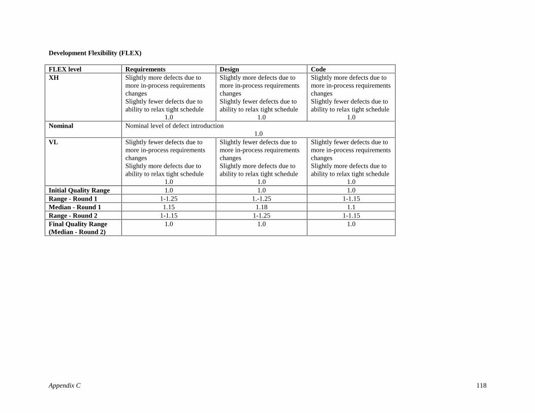
Appendix C 118
Development Flexibility (FLEX)
FLEX level Requirements Design CodeXH Slightly more defects due to
more in-process requirementschangesSlightly fewer defects due toability to relax tight schedule
1.0
Slightly more defects due tomore in-process requirementschangesSlightly fewer defects due toability to relax tight schedule
1.0
Slightly more defects due tomore in-process requirementschangesSlightly fewer defects due toability to relax tight schedule
1.0Nominal Nominal level of defect introduction
1.0VL Slightly fewer defects due to
more in-process requirementschangesSlightly more defects due toability to relax tight schedule
1.0
Slightly fewer defects due tomore in-process requirementschangesSlightly more defects due toability to relax tight schedule
1.0
Slightly fewer defects due tomore in-process requirementschangesSlightly more defects due toability to relax tight schedule
1.0Initial Quality Range 1.0 1.0 1.0Range - Round 1 1-1.25 1.-1.25 1-1.15Median - Round 1 1.15 1.18 1.1Range - Round 2 1-1.15 1-1.25 1-1.15Final Quality Range(Median - Round 2)
1.0 1.0 1.0
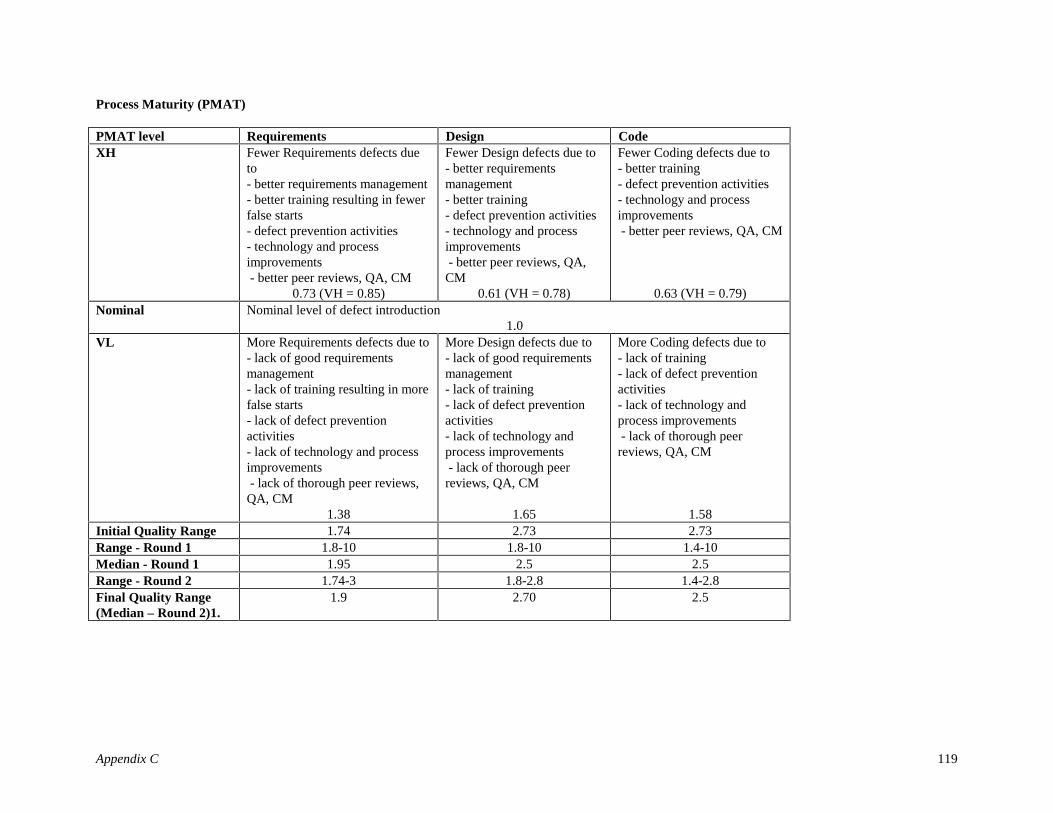
Appendix C 119
Process Maturity (PMAT)
PMAT level Requirements Design CodeXH Fewer Requirements defects due
to- better requirements management- better training resulting in fewerfalse starts- defect prevention activities- technology and processimprovements - better peer reviews, QA, CM
0.73 (VH = 0.85)
Fewer Design defects due to- better requirementsmanagement- better training- defect prevention activities- technology and processimprovements - better peer reviews, QA,CM
0.61 (VH = 0.78)
Fewer Coding defects due to- better training- defect prevention activities- technology and processimprovements - better peer reviews, QA, CM
0.63 (VH = 0.79)Nominal Nominal level of defect introduction
1.0VL More Requirements defects due to
- lack of good requirementsmanagement- lack of training resulting in morefalse starts- lack of defect preventionactivities- lack of technology and processimprovements - lack of thorough peer reviews,QA, CM
1.38
More Design defects due to- lack of good requirementsmanagement- lack of training- lack of defect preventionactivities- lack of technology andprocess improvements - lack of thorough peerreviews, QA, CM
1.65
More Coding defects due to- lack of training- lack of defect preventionactivities- lack of technology andprocess improvements - lack of thorough peerreviews, QA, CM
1.58Initial Quality Range 1.74 2.73 2.73Range - Round 1 1.8-10 1.8-10 1.4-10Median - Round 1 1.95 2.5 2.5Range - Round 2 1.74-3 1.8-2.8 1.4-2.8Final Quality Range(Median – Round 2)1.
1.9 2.70 2.5

Appendix C 120

Appendix D 123
Appendix D: Defect Removal Model Behavioral Analysis
Personnel Factors (PERS)
PERS level Requirements Design CodeXH More Requirements defects
removed due to betterunderstanding and higherconsistency
90%
More Requirements defects removeddue to easier traceabilityMore Design defects removed due tohigher consistency
90%
More Coding defects removed dueto fewer missing guidelines andambiguities
90%Nominal Nominal level of defect introduction
50%XL Fewer Requirements defects
removed due to lowerunderstanding and lowerconsistency
30%
Fewer Requirements defects removeddue to less efficient traceabilityFewer Design defects removed due tolower consistency
30%
Fewer Coding defects removed dueto missing guidelines andambiguities
40%Quality Range 30-90% 30-90% 40-90%
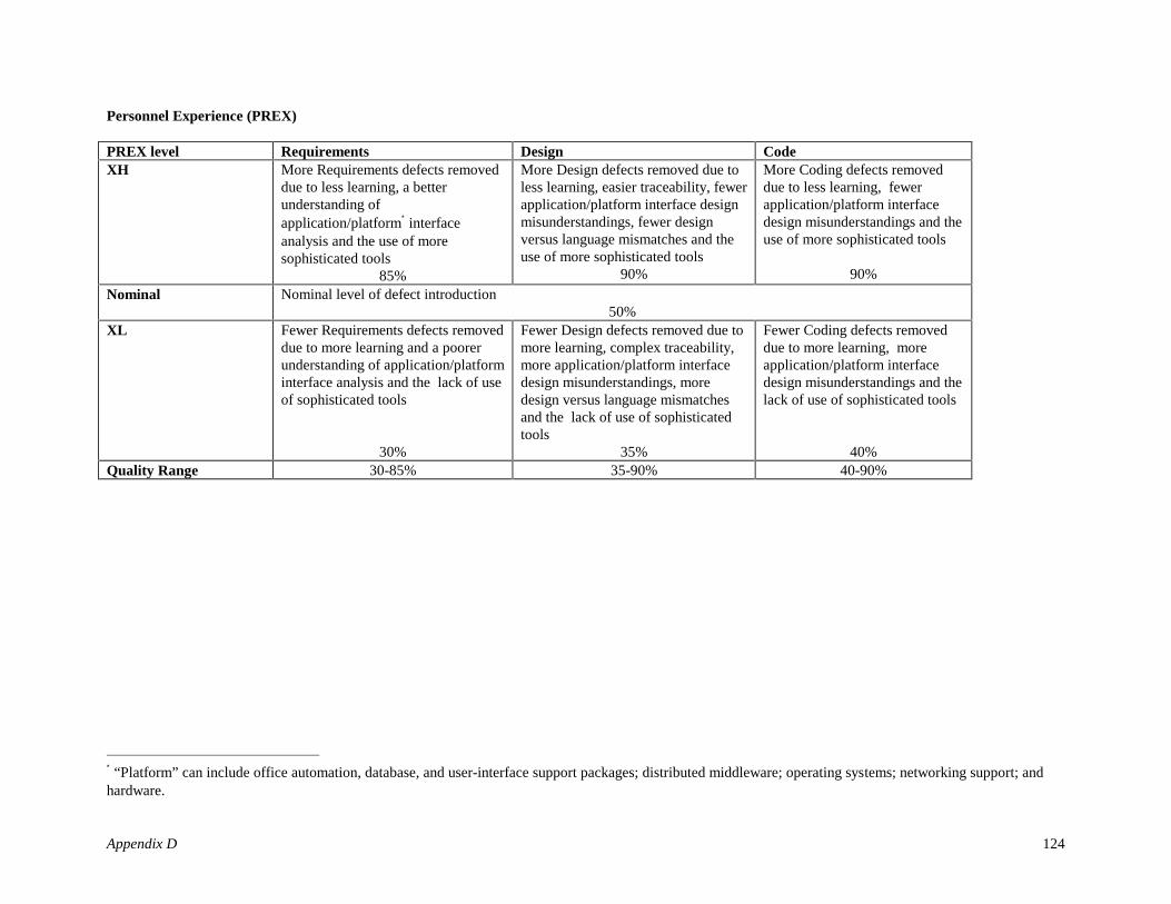
Appendix D 124
Personnel Experience (PREX)
PREX level Requirements Design CodeXH More Requirements defects removed
due to less learning, a betterunderstanding ofapplication/platform∗ interfaceanalysis and the use of moresophisticated tools
85%
More Design defects removed due toless learning, easier traceability, fewerapplication/platform interface designmisunderstandings, fewer designversus language mismatches and theuse of more sophisticated tools
90%
More Coding defects removeddue to less learning, fewerapplication/platform interfacedesign misunderstandings and theuse of more sophisticated tools
90%Nominal Nominal level of defect introduction
50%XL Fewer Requirements defects removed
due to more learning and a poorerunderstanding of application/platforminterface analysis and the lack of useof sophisticated tools
30%
Fewer Design defects removed due tomore learning, complex traceability,more application/platform interfacedesign misunderstandings, moredesign versus language mismatchesand the lack of use of sophisticatedtools
35%
Fewer Coding defects removeddue to more learning, moreapplication/platform interfacedesign misunderstandings and thelack of use of sophisticated tools
40%Quality Range 30-85% 35-90% 40-90%
∗ “Platform” can include office automation, database, and user-interface support packages; distributed middleware; operating systems; networking support; andhardware.

Appendix D 125
Use of Software Tools (TOOL)
TOOL level Requirements Design CodeVH More Requirements defects
removed as easier to find and fixvia tools
70%
More Design defects removedas easier to fix and find viatools
75%
More Coding defectsremoved as easier to findand fix via tools
85%Nominal Nominal level of defect introduction
50%VL Fewer Requirements defects
removed as harder to find and fixvia tools
20%
Fewer Design defectsremoved as harder to find andfix via tools
25%
Fewer Coding defectsremoved as harder to findand fix via tools
30%Quality Range 20-70% 25-75% 30-85%

Appendix D 126
Required Software Reliability (RELY)
RELY level Requirements Design CodeVH More Requirements defects removed
due to more consistency, detailedverification, QA, CM, standards, SSR,documentation, IV&V interface, testplans, procedures
90%
More Design defects removed dueto detailed verification, QA, CM,standards, PDR, documentation,IV&V interface, design inspections,test plans, procedures
95%
More Coding defects removed due todetailed verification, QA, CM,standards, documentation, IV&Vinterface, code inspections, test plans,procedures
95%Nominal Nominal level of defect introduction
50%VL Fewer Requirements defects removed
due to lower consistency, minimalverification, QA, CM, standards, SSR,documentation, IV&V interface, testplans, procedures
25%
Fewer Design defects due tominimal verification, QA, CM,standards, PDR, documentation,IV&V interface, design inspections,test plans, procedures
25%
Fewer Coding defects removed due tominimal verification, QA, CM,standards, PDR, documentation, IV&Vinterface, code inspections, test plans,procedures
25%Quality Range 25-90% 25-95% 25-95%
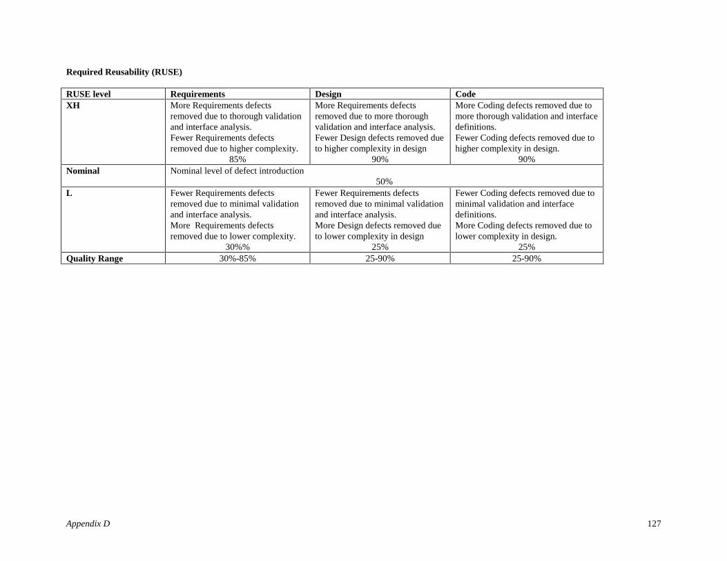
Appendix D 127
Required Reusability (RUSE)
RUSE level Requirements Design CodeXH More Requirements defects
removed due to thorough validationand interface analysis.Fewer Requirements defectsremoved due to higher complexity.
85%
More Requirements defectsremoved due to more thoroughvalidation and interface analysis.Fewer Design defects removed dueto higher complexity in design
90%
More Coding defects removed due tomore thorough validation and interfacedefinitions.Fewer Coding defects removed due tohigher complexity in design.
90%Nominal Nominal level of defect introduction
50%L Fewer Requirements defects
removed due to minimal validationand interface analysis.More Requirements defectsremoved due to lower complexity.
30%%
Fewer Requirements defectsremoved due to minimal validationand interface analysis.More Design defects removed dueto lower complexity in design
25%
Fewer Coding defects removed due tominimal validation and interfacedefinitions.More Coding defects removed due tolower complexity in design.
25%Quality Range 30%-85% 25-90% 25-90%

Appendix D 128
Product Complexity (CPLX)
CPLX level Requirements Design CodeXH Fewer Requirements defects removed due to
lack of thorough understandingFewer Requirements Defects removed due to - complex specification and validation - complex interfaces
30%
Fewer Design defects removeddue to - complex design and validation - complex interfaces
25%
Fewer Coding defects removeddue to - complex data and controlstructures - complex interfaces
25%Nominal Nominal level of defect introduction
50%VL More Requirements defects removed due to
thorough understandingMore Requirements Defects removed due to - simpler specification and validation - simpler interfaces
75%
More Design defects removed dueto - simpler design and validation - simpler interfaces
75%
More Coding defects removed dueto - simpler data and controlstructures - simpler interfaces
75%Quality Range 30-75% 25-75% 25-75%

Appendix D 129
Disciplined Methods (DISC)* - e.g. Cleanroom, PSP
DISC level Requirements Design CodeVH More Requirements defects
removed due to- more thorough specs- more emphasis on defectprevention
90%
More Design defects removed due to- more thorough specs- more emphasis on defect prevention
90%
More Coding defects removed due to- extensive self-review- more emphasis on defect prevention- extensive defect checklists- defensive programming- independent unit testing
90%Nominal Nominal level of defect introduction
50%Quality Range 50-90% 50-90% 50-90%
* This Defect Driver is in addition to the 22 COCOMO II drivers

Appendix D 130
Architecture/Risk Resolution (RESL)
RESL level Requirements Design CodeXH More Requirements defects removed due
to - fewer number of highly critical riskitems - very little uncertainty in keyarchitecture drivers : mission userinterface, COTS, hardware, technology,performance - thorough planning, specs, reviews andvalidation
85%
More Design defects removed due to - fewer number of highly critical riskitems - very little uncertainty in keyarchitecture drivers : mission userinterface, COTS, hardware,technology, performance - thorough planning, specs. reviewsand validation
90%
More Coding defects removed due to - fewer number of highly critical riskitems - very little uncertainty in keyarchitecture drivers : mission userinterface, COTS, hardware, technology,performance - fewer misunderstandings in interpretingincomplete or ambiguous specs
85%Nominal Nominal level of defect introduction
50%VL Fewer Requirements defects removed
due to - higher number of highly critical riskitems - high uncertainty in key architecturedrivers : mission user interface, COTS,hardware, technology, performance - minimal planning, specs, reviews andvalidation
30%
Fewer Design defects removed due to - higher number of highly criticalrisk items - high uncertainty in key architecturedrivers : mission user interface,COTS, hardware, technology,performance - minimal planning, specs, reviewsand validation
30%
Fewer Coding defects removed due to - higher number of highly critical riskitems - high uncertainty in key architecturedrivers : mission user interface, COTS,hardware, technology, performance - minimal planning, specs, reviews andvalidation- more misunderstandings in interpretingincomplete or ambiguous specs
30%Quality Range 30-85% 30-90% 30-85%

Appendix D 131
Process Maturity (PMAT)
PMAT level Requirements Design CodeXH More Requirements defects removed due
to- better requirements management- better training resulting in fewer falsestarts- defect prevention activities- technology and process improvements - better peer reviews, QA, CM
85%
More Design defects removed due to- better requirements management- better training- defect prevention activities- technology and processimprovements - better peer reviews, QA, CM
90%
More Coding defects removed dueto- better training- defect prevention activities- technology and processimprovements - better peer reviews, QA, CM
90%Nominal Nominal level of defect introduction
50%VL Fewer Requirements defects removed due
to- lack of good requirements management- lack of training resulting in more falsestarts- lack of defect prevention activities- lack of technology and processimprovements - lack of thorough peer reviews, QA, CM
25%
Fewer Design defects removed due to- lack of good requirementsmanagement- lack of training- lack of defect prevention activities- lack of technology and processimprovements - lack of thorough peer reviews, QA,CM
30%
Fewer Coding defects removed dueto- lack of training- lack of defect prevention activities- lack of technology and processimprovements - lack of thorough peer reviews,QA, CM
25%Quality Range 25-85% 30-90% 25-90%

Appendix D 132