income and subjective well-being: a case study boo mei

Kajian Malaysia, Vol. 38, No. 2, 2020, 91–114

© Penerbit Universiti Sains Malaysia, 2020. This work is licensed under the terms of the Creative Commons Attribution (CC BY) (http://creativecommons.org/licenses/by/4.0/).

INCOME AND SUBJECTIVE WELL-BEING: A CASE STUDY

Boo Mei Chin1*, Yen Siew Hwa2 and Lim Hock Eam3

1Economics and Corporate Administration Division, Universiti Kolej Tunku Abdul Rahman, Pulau Pinang, MALAYSIA 2School of Distance Education (Economics Section), Universiti Sains Malaysia, Pulau Pinang, MALAYSIA3Economics Department, College of Business, Universiti Utara Malaysia, Kedah, MALAYSIA*Corresponding author: [email protected]

Published online: 30 October 2020 To cite this article: Boo, M.C., S.H. Yen and H.E. Lim. 2020. Income and subjective well-being: A case study. Kajian Malaysia 38(2): 91–114. https://doi.org/10.21315/km2020.38.2.4To link to this article: https://doi.org/10.21315/km2020.38.2.4

ABSTRACT

This article examines to what extent income could influence subjective well-being based on a case study involving 249 working adult students from the School of Distance Education at Universiti Sains Malaysia (USM). Subjective well-being is represented by the respondent’s level of happiness and life satisfaction. The outcomes show happiness and life satisfaction are affected by household income, relative income, expected income and health. Household income seems to matter more in influencing both happiness and life satisfaction as compared to relative income. Respondents are less happy and less satisfied when the gap between their actual and expected income became larger. This study shows that better health status increases one’s happiness and life satisfaction. Being divorced, separated or widowed compared to being single shows an adverse impact on their happiness but has no significant influence on their life satisfaction. Age and life satisfaction displayed an inverted U-shaped relationship indicating that life satisfaction among the respondents reaches its peak at age 44 and starts to decline after that. The Malays seemed to be more satisfied with their lives as compared with the other ethnic groups.

Keywords: income, subjective well-being, happiness, life satisfaction

Boo Mei Chin et al.

92

INTRODUCTION

There is scholarly and policy concern about whether rising income leads to improvement in subjective well-being among individuals. Some argued that income could affect subjective well-being, but others suggested otherwise. In the early studies carried out by Easterlin (1974), he found that economic growth does not improve the average subjective well-being at a country level. This has sparked a debate on income-happiness paradox, also known as “Easterlin Paradox”. Easterlin Paradox indicates that richer individuals are happier than poorer ones, yet raising higher income for all does not compensate with the levels of happiness.

This study aims to examine the influence of income on the subjective well-being of Malaysians represented by a case study among working adult students at the School of Distance Education, Universiti Sains Malaysia (USM). Our study examines the relationship between subjective well-being, represented by happiness and life satisfaction, and income in different perspectives, absolute, relative and expected. The analysis also includes the effects of non-material factors on subjective well-being such as age, gender, health, ethnicity and marital status.

Subjective well-being is defined as a general evaluation of a person’s life (Diener and Seligman 2002). It concerns the respondents’ personal judgement evaluative response to various aspects of a person’s life (Frey and Stutzer 2002b). Researchers have asserted that happiness and life satisfaction (which form part of a subjective well-being construct) are generally considered to be synonymous (Easterlin 2001; Brockmann and Delhey 2010; Leung et al. 2011). However, others proclaimed happiness and life satisfaction can be defined in different ways because both may be influenced by different domains of people’s lives (Cummins 1998; Frey and Stutzer 2002a). Happiness is an immediate, short term, temporary and retrospective mental state, whereas life satisfaction is a relatively long-term judgement of individual well-being (Gamble and Gärling 2012; Chui and Wong 2016).

Malaysia inherited a multiracial and multicultural society. Although the people are striving for material wealth, it is uncertain whether the overall well-being has actually improved among the society. Easterlin (2001), Frey and Stutzer (2002a) asserted that an increase in income only yields a slight increase in happiness notably among those in the higher income groups. However, Veenhoven and Vergunst (2014) defended that income growth in nations goes with rising happiness particularly nations with higher economic growth had higher average happiness. In developed nations, Blanchflower and Oswald (2004) revealed that relative income, as the ratio of a person income to the state income per capita had greater effect upon human well-being compared to absolute income. Yu and Chen (2016) found that the effect of income on well-being at individual-level was different from that at country-level in China. At individual-level, household income

Income and Subjective Well-Being

93

was significantly associated with happiness and life satisfaction. On the contrary, at the country level, only relative income was associated with happiness and life satisfaction. Studies that examined the association between absolute income and relative income on happiness include Blanchflower and Oswald (2004), Oshio, Nozaki and Kobayashi (2011), Yu and Chen (2016), while others extended the influence of expected income on happiness (Caner 2015; Tsui 2014). Literature on happiness that involved other socio-demographic factors (Tambyah and Tan 2011; Howell et al. 2012; Yiengprugsawan et al. 2012), social capital (Leung et al. 2011), elderly population (Eshkoor et al. 2015) and gender (Chui and Wong 2016).

This study hopes to provide a more comprehensive coverage particularly in examining the relationship between different types of income (absolute, relative and expected) and subjective well-being in Malaysia. It further extends to examine the effect of income on happiness and life satisfaction across the three income groups of B40, M40 and T20.1

There have been great concerns among policy makers and scholars, whether economic growth is adequate in gauging a country’s performance. Whether income has more influence over the level of subjective well-being could be a crucial matter to look into for better public policy measures. Studies on the economics of happiness not only contribute to research on well-being, it also enriches the scope of behavioural economics studies. There is a great potential to apprehend mental, social and physical well-being that could contribute to a more holistic growth in national well-being.

LITERATURE REVIEW

National income may not be a reliable measure to societal well-being. Easterlin (1974) found that well-being was not substantially related to the economic growth in United States. In an article entitled “Will raising the income of all increase the happiness of all?” by Easterlin (1995), he found that, overtime, there was only minimal increase in happiness relative to remarkable increased in incomes and living standards. His studies covered the periods between 1972 and 1991 for United States, 1973–1989 for the nine European countries, and 1958–1987 for Japan. In a cross-sectional analysis, Easterlin and Angelescu (2009) found that rich and poor countries experienced satisfaction in life increased proportionally to absolute amount of GDP per capita but at diminishing rate. Easterlin (2013) repeated the study and reiterated that happiness and income are not related in the long run although there are short-term fluctuations in happiness and income which were positively related.

Subjective well-being may depend on absolute income and relative income. The influence of absolute income on happiness refers to the ability of money in

Boo Mei Chin et al.

94

buying things that brings happiness such as material goods, experiences, and even the feelings of security while relative income refers to a person whether he or she has either more or less income compare to others (Cheung and Lucas 2016). As shown in Sacks, Stevenson and Wolfers (2010), absolute income has great influence on well-being. Their study went beyond individuals’ level of happiness and they further investigated well-being between countries; the results showed that the greater GDP per capita, the higher level of average life satisfaction. The magnitude of the satisfaction-income gradient was found to be about the same whether comparisons were made among individuals within a country or between countries.

According to the relative income hypothesis, the happiness or satisfaction level of an individual seemed to depend more on relative income rather than absolute income (Clark and Oswald 1996). Graham and Felton (2006) used an annual survey provided by the Latinobarometro Corporation, a non-profit organisation in Chile, to explore the effects of absolute and relative income on happiness based on income quintile of respondents in Latin American countries. They found that relative income had positive significant impact on happiness but not absolute income. Studies that found significant influence of relative income on happiness include McBride (2001) in America, Ferrer-i-Carbonell (2005) in Germany, and Stutzer (2004) in Switzerland.

A survey carried out by Solnick and Hemenway (1998) at the Harvard’s School of Public Health to gauge if relative income matters more than absolute income. It involved 159 students and 79 faculty members and staff. Their intention was to determine the importance of positional concerns among the respondents. The question was designed as follows:

There are two states of the world (State A and State B). You are asked to pick which of the two you would prefer to live in:

“State A: Your current yearly income is $50,000; others earn $25,000”

“State B: Your current yearly income is $100,000; others earn $200,000”

From the two states, the respondents were asked to choose whether they prefer to live in a society where their annual income is $50,000 while others, an average person earning an income of $25,000 or in one where they have an annual income of $100,000 while others, on the average earning $200,000 (prices and purchasing power of money were same in both states). What can be interpreted here is that,


95

if a respondent chose State A, relative income matters but if State B is preferred, absolute income matters more.

Some studies considered the influence of expected income on happiness. According to Easterlin (1995), the impact of income on individual’s subjective well-being depends on changing standards based on their expectations. On average, people believed that they have been worse off in the past and they will be better off in the future based on their current level of happiness (Easterlin 2001).

Based on cross-sectional data from Turkish Life Satisfaction Survey between 2003 and 2011, Caner (2015) found a positive association between expectations of future household income and happiness among the Turkish society. The results indicated that an increased in one’s expected household income contributed to higher happiness. However, a declined in one’s expected household income was associated with lower happiness. Therefore, being optimistic about one’s expectations of future household income promotes happiness in Turkey. The author also highlighted that life circumstances such as health and employment made greater contribution to happiness than income in the Turkish society.

Oshio, Nozaki and Kobayashi (2011) defined relative income as the gap between an individual or household income and the average income of the reference group. Their perceived happiness study was based on data obtained from the General Social Survey conducted in 2006 that involved three nations; China, Japan and Korea. Their findings showed that the associations between relative income and happiness were stronger for individual income as compared to family income in China, but not for Japan and Korea.

Tsui (2014) indicated that Taiwanese seemed to be less happy when their actual incomes were lower than expected incomes. Another interesting discovery was happiness does not only depend on one’s absolute but relative income. A negative relationship between relative income and happiness among the Taiwanese shows that happiness decreases when the gap between one’s incomes compared to those with higher income widens. At the same time, when compared with those with lower income, as the income gap narrows one’s happiness also reduces.

There are limited studies on happiness among the society in Malaysia. Redhwan et al. (2010) examined how individual perceived the contributing factors on their happiness. They conducted a study at the Management and Science University, Shah Alam and the sample size was limited to 33 medical science students. Their study indicated that money is the main source of happiness followed by having good friends and relatives. Some gave priority to stability of life as well as good health and only a few responded that success in life as main contributor to happiness. Ang and Abu Talib (2011) is another study which reaffirmed that materialism as the main contributor to life satisfaction among higher education institutions students.

Boo Mei Chin et al.

96

Income may not be the only factor that contributes to subjective well-being. Some studies have posited a U-shaped relationship between age and subjective well-being, indicating that middle age was less happy than those younger or older people (Clark and Oswald 1994; Helliwell 2002; Blanchflower and Oswald 2008; Dolan, Peasgood and White 2008). On the contrary, Easterlin (2006) pointed out that happiness is at the greatest at midlife, progressing from age 18 to 51, and declining thereafter.

Tambyah and Tan (2011) showed that only Malaysian males were happier than their female counterparts when investigating happiness among people in the ASEAN-5 countries. Some claimed that gender and age were insignificant determinants of life satisfaction (Ngoo, Tey and Tan 2015). In addition, health status has been described as an influential predictor of subjective well-being (Wu and Schimmele 2006; Howell et al. 2012; Lam and Liu 2014). Married people were found to be happier than those of other marital status (Diener 1984; Stutzer and Frey 2006). Eshkoor et al. (2015) indicated that the Malays were more satisfied with their lives as compared to the non-Malays. Their study was based on elderly population in Malaysia.

To access the well-being of society, Helliwell (2008) suggested a direct approach of question whereby respondents were directly asked to evaluate the quality of their lives. Subjective well-being has been generally referred to as cognitive evaluations of a person’s life which can be gauged by using questions on individual’s happiness or life satisfaction.

DATA AND METHODOLOGY

This case study involves 249 distance learning students from the School of Distance Education at USM. Two hundred and fifty respondents are chosen in the study out of a population size of slightly below 6,000 active students during the academic year of 2015/2016. This indicates a sample size for a precision level of ± 6% where the confidence level is 95% (more or less a sample size of 260).2 One of the respondents was dropped due to incomplete questionnaire. Distance education students were chosen because most of them are income earners. There are relatively good representatives in terms of age, ethnic group, religion, place of origin, marital status and gender. Convenience sampling method is used.

For this case study, we apply a more direct approach using “single question” to measure happiness and life satisfaction which is adapted from World Values Survey (WVS). The questions were presented in both languages, English and bahasa Malaysia. Respondents were required to rate their happiness levels. The respective ratings were based on a Likert scale that ranges from “1” as being not happy at all to “7” as very happy. Respondents were also asked to indicate their


97

life satisfaction levels on a scale that set from “1” as completely dissatisfied to “7” as completely satisfied. The difference in the points represent the degree of order of the continuum (smaller to larger) that set by the scale (Sekaran 2003). We chose a standardised Likert scale of seven, instead of four and ten for the happiness and life satisfaction questions respectively based on the WVS. A standardised scale for the dependent variables allows a more straight forward comparisons between the two models in the analysis. This single item measurement has been found to have good validity and reliability (for instance, see Cheung and Lucas 2014; Cummins 1995). Nevertheless, it is important to note that the happiness measurement using experimental approach (such as Kugler, Connolly and Ordonez 2010) could be a good alternative measurement.

A pilot test was carried out on 25 January 2016. Forty-eight respondents (1 Indian, 6 Chinese, 6 others and the rest were Malays) voluntarily participated in the pilot test. No major corrections were needed for the questionnaire as the pilot test showed that it was clearly understood by the participants.

An online survey was carried out to collect data among the USM undergraduate students at the School of Distance Education. The questionnaire was formatted using Google Forms, which offered a form option that can be used to generate online surveys. The questionnaire was uploaded online at the School of Distance Education, USM, e-portal site from 21 March to 1 August 2016. Two hundred and one students responded online. Since there was no major correction in the questionnaire, all the data collected during the pilot test were included in the analysis.

Some of the observations were omitted as a result of missing data or suspicious responses given by the respondents, particularly information regarding their incomes. Only 235 respondents revealed their household income, 248 and 242 respondents stated their personal income and expected income respectively. Eventually, only 230 respondents revealed all the three incomes. Thus, the final sample size that was used in the analysis of happiness and life satisfaction models is 230.

The data for happiness and life satisfaction in this study are in ordinal form. Thus, an appropriate method to use in the analysis is the ordered logit regression. The maximum likelihood estimation based on ordered logit regression gauges the optimum set of coefficients for predicting values of the logit-transformed probability of the dependent variable being in one particular category rather than another. Ordered logit specification can be represented in the form of a latent regression model as follow:

m

i = 1y* = ∑ βixi + ɛ

Boo Mei Chin et al.

98

y*: unobserved latent variable; xs: independent variables; ɛ: error term. The observed ordinal variable (y) has values between one and k, as follow:

y1 = j ⇔ αj–y< y1* ≤ αk for completeness, α0 = –∞ and αk = +∞

where αs are the unknown threshold parameters separating the adjacent ordinal categories (j). The probability of y observing a value of j is:

Pij = Pr(y = j) = Pr(αj–1 < y* ≤ αj) = Pr(αj–1 < m

i = 1∑ βixi + ɛ ≤ αj)

The error term, ɛ, is assumed to be logistically distributed. The dependent variable, y, which represents happiness and life satisfaction in this study has the values k = 1 to 7.

Both the happiness (Model 1) and life satisfaction (Model 2) models were tested for goodness of fit using various tests. All covariates’ coefficients are found to be significant at the 1% level based on the overall fit tests on null hypothesis. Models 1 and 2 have 35.74% and 28.11% of accuracy in prediction respectively which are substantially higher than the equal proportion of seven categories (14.29%). To test the existence of multicollinearity, all insignificant independent variables (based on t-test) are tested for joint insignificance. They were found to be jointly insignificant in both Models 1 and 2 with p-value of 0.5494 and 0.5835, respectively. The estimated ordered logit models can thus be concluded as to have high goodness of fit statistically.3

The seven steps Likert scales is commonly employed to measure personal evaluation. Finstad (2010) suggested that seven-point Likert items produced a more accurate and a better reflection of respondent’s true evaluation than five-point Likert items or even higher-order items. The Likert scale was widely used to measure subjective well-being and its validity and reliability had been supported across various cultural contexts (Diener, Inglehart and Tay 2013).

DESCRIPTIVE STATISTICS

Table 1 presents the description of the variables used in the analyses. Table 2a shows the mean and standard deviation of happiness, life satisfaction, age and different types of income. Table 2b displays the respondents’ characteristics based on mean happiness and life satisfaction. This survey solicits information about household income, comparison income and expected income, age, gender, marital status, health and ethnicity.


99

Table 1: Description of variables used in the analysesVariables Description and coding

Happiness Taking all things together, would you say you are: (scale “1” to “7”; 1 representing not happy at all, 7 representing very happy)

Life satisfaction All things considered, how satisfied are you with your life as a whole these days? (scale “1” to “7”; 1 representing completely dissatisfied, 7 representing completely satisfied)

Various income

Household income Monthly household gross income (in RM)

Relative income Respondent’s preference of income as compared to his or her peers:State A: Your current yearly income is RM50,000; others earn RM25,000 (coded as 1)State B: Your current yearly income is RM100,000; others earn RM200,000 (coded as 0)

Expected income The difference between one’s expected income and personal income

Age

Age Age in years

Age sq Age squared

Gender

Female Female (coded as 1, 0 otherwise)

Male* Male

Marital status

Married Married (coded as 1, 0 otherwise)

Divorced/separated/widowed

Divorced, separated and widowed (coded as 1, 0 otherwise)

Single* Single

State of health (subjective)

Very healthy Very healthy (coded as 1, 0 otherwise)

Healthy Healthy (coded as 1, 0 otherwise)

Not healthy* Fair and poor health

Ethnic

Malay Malay (coded as 1, 0 otherwise)

Chinese Chinese (coded as 1, 0 otherwise)

Others* Indian and othersNote: *refer to reference group.

Boo Mei Chin et al.

100

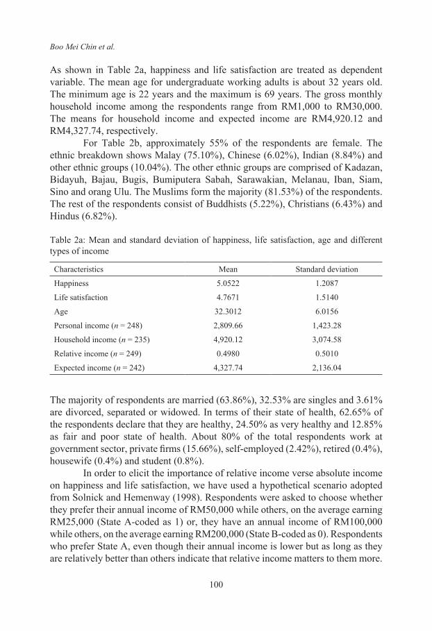
As shown in Table 2a, happiness and life satisfaction are treated as dependent variable. The mean age for undergraduate working adults is about 32 years old. The minimum age is 22 years and the maximum is 69 years. The gross monthly household income among the respondents range from RM1,000 to RM30,000. The means for household income and expected income are RM4,920.12 and RM4,327.74, respectively.

For Table 2b, approximately 55% of the respondents are female. The ethnic breakdown shows Malay (75.10%), Chinese (6.02%), Indian (8.84%) and other ethnic groups (10.04%). The other ethnic groups are comprised of Kadazan, Bidayuh, Bajau, Bugis, Bumiputera Sabah, Sarawakian, Melanau, Iban, Siam, Sino and orang Ulu. The Muslims form the majority (81.53%) of the respondents. The rest of the respondents consist of Buddhists (5.22%), Christians (6.43%) and Hindus (6.82%).

Table 2a: Mean and standard deviation of happiness, life satisfaction, age and different types of income

Characteristics Mean Standard deviation

Happiness 5.0522 1.2087

Life satisfaction 4.7671 1.5140

Age 32.3012 6.0156

Personal income (n = 248) 2,809.66 1,423.28

Household income (n = 235) 4,920.12 3,074.58

Relative income (n = 249) 0.4980 0.5010

Expected income (n = 242) 4,327.74 2,136.04

The majority of respondents are married (63.86%), 32.53% are singles and 3.61% are divorced, separated or widowed. In terms of their state of health, 62.65% of the respondents declare that they are healthy, 24.50% as very healthy and 12.85% as fair and poor state of health. About 80% of the total respondents work at government sector, private firms (15.66%), self-employed (2.42%), retired (0.4%), housewife (0.4%) and student (0.8%).

In order to elicit the importance of relative income verse absolute income on happiness and life satisfaction, we have used a hypothetical scenario adopted from Solnick and Hemenway (1998). Respondents were asked to choose whether they prefer their annual income of RM50,000 while others, on the average earning RM25,000 (State A-coded as 1) or, they have an annual income of RM100,000 while others, on the average earning RM200,000 (State B-coded as 0). Respondents who prefer State A, even though their annual income is lower but as long as they are relatively better than others indicate that relative income matters to them more.


101

On the other hand, respondents who chose State B where they prefer higher income even though the real purchasing power is 50% less than the others in the society indicate that absolute income is more important to them.

Table 2b: Respondents’ characteristics based on mean happiness and life satisfaction

Categorical variables

Percentage

Mean happiness Mean life satisfaction Total

<5.05 >5.05 <4.77 >4.77

Relative income

State A(Your current yearly income is RM50,000; others earn RM25,000)

53.55 43.62 54.84 46.79 49.80

State B(Your current yearly income is RM100,000; others earn RM200,000)

46.45 56.38 45.16 53.21 50.20

Gender

Female 52.26 58.51 54.84 54.49 54.62

Male 47.74 41.49 45.16 45.51 45.38

Ethnic

Malay 74.19 76.60 72.04 76.92 75.10

Chinese 7.10 4.26 5.38 6.41 6.02

Indian 7.10 11.70 6.02 10.75 8.84

Others 11.61 7.44 16.56 5.92 10.04

Marital status

Single 32.26 32.98 33.33 32.05 32.53

Married 61.94 67.02 60.22 66.03 63.86

Divorced/separated/widowed 5.80 0.00 6.45 1.92 3.61


Very good 23.23 26.60 24.73 24.36 24.50

Good 61.94 63.83 56.99 66.03 62.65

Fair and poor 14.83 9.57 18.28 9.61 12.85

Expected income refers to the respondent’s expected monthly income based on his or her qualifications and experiences. It is measured by asking the respondent: “Given your qualification and experiences, what is your expected monthly income?” The variable expected income in the analysis is defined as the difference between one’s personal monthly income and the expected monthly income.

Boo Mei Chin et al.

102

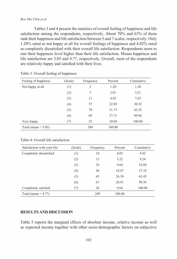
Tables 3 and 4 present the statistics of overall feeling of happiness and life satisfaction among the respondents, respectively. About 70% and 63% of them rank their happiness and life satisfaction between 5 and 7 scales, respectively. Only 1.20% rated as not happy at all for overall feelings of happiness and 4.02% rated as completely dissatisfied with their overall life satisfaction. Respondents seem to rate their happiness level higher than their life satisfaction. Means happiness and life satisfaction are 5.05 and 4.77, respectively. Overall, most of the respondents are relatively happy and satisfied with their lives.

Table 3: Overall feeling of happiness

Feeling of happiness (Scale) Frequency Percent Cumulative

Not happy at all (1) 3 1.20 1.20

(2) 5 2.01 3.21

(3) 11 4.42 7.63

(4) 57 22.89 30.52

(5) 79 31.73 62.25

(6) 69 27.71 89.96

Very happy (7) 25 10.04 100.00

Total (mean = 5.05) 249 100.00

Table 4: Overall life satisfaction

Satisfaction with your life (Scale) Frequency Percent Cumulative

Completely dissatisfied (1) 10 4.02 4.02

(2) 13 5.22 9.24

(3) 24 9.64 18.88

(4) 46 18.47 37.35

(5) 65 26.10 63.45

(6) 67 26.91 90.36

Completely satisfied (7) 24 9.64 100.00

Total (mean = 4.77) 249 100.00

RESULTS AND DISCUSSION

Table 5 reports the marginal effects of absolute income, relative income as well as expected income together with other socio-demographic factors on subjective


103

well-being based on the ordered logit regression. Model 1 shows the marginal effects of the explanatory variables on happiness whereas, Model 2 displays the effects of the explanatory variables on life satisfaction.

Model 1 shows that household income, relative income and expected income have significant contribution to happiness. A unit increase in household income will increase the probability of being happier by 1.03%, holding other variables at their mean values.

As for the influence of relative income in subjective well-being, among the respondents, there is no significant difference between the two choices: 49.8% of the respondents have chosen State A and the remaining chose State B. Our study is to gauge if their choices have any influence on their subjective well-being. Our outcome indicated a negative and significant relationship with happiness and life satisfaction. That can be interpreted as, those who are happier or more satisfied in life have the tendency to choose State B which indicates that absolute income is more important to them rather than relative income. As long as they earn high absolute income even though relatively less than others, they are happier.

Our outcome shows a significant negative result between expected income (measured by the difference between expected income and the actual personal income) and subjective well-being. When there is one unit increase in expected income, it decreases the probability of being happier by 2.21%, holding other variables at their mean values respectively. It shows as the extent of difference between expected and actual income gets larger, happiness and life satisfaction fall. Thus, indicating that respondents who feel that he or she deserves, based on their qualification and experiences, to get much more than they are currently paid, they are less happy or satisfied. On the other hand, those who feel that they are paid quite closed to what they deserve are happier and satisfied.

Besides income, this study also investigates the influence of other variables on happiness. Those who are divorced, separated or widowed compared to the singles have adverse effects on happiness. The marginal effects show that happiness of those who are divorced, separated or widowed decreases by 25% compared to those who are single, holding other variables at their mean values. This finding is similar to Yiengprugsawan et al. (2012) who found that separated, divorced or widowed were the least happy among the cohort of distance learning students from Open University in Thailand. Those who are married are less happy as compared to the singles but the result is insignificant. About 65% among the cohort of USM distance learning adults are married. For those who are married, pursuing higher education and at the same time striking the balance between work and family can be very challenging tasks and that could have adversely affected their happiness levels.

Being very healthy is statistically significant and positively related to happiness. This result shows that those who are very healthy compared to not

Boo Mei Chin et al.

104

healthy have higher probability of being happier by 10.92%, holding other variables at their mean values.

Model 2 in Table 5 reports the marginal effects of income and other socio-demographic factors on life satisfaction. Household absolute income, relative income and expected income have significant contribution to life satisfaction. It shows that a unit increase in household income will increase the probability of being happier by 1.95 %, holding other variables at their mean values. This study reaffirms that absolute income contributes to one’s happiness and life satisfaction levels. These findings lend support to Stevenson and Wolfers (2008) who asserted the significant role of absolute income in determining the subjective well-being of people.

Table 5: Marginal effects of happiness and life satisfaction (ordered logit estimations)

VariablesModel 1 (Happiness) Model 2 (Life satisfaction)

C M SD C M SD

Income

Household income 0.0669 0.0103 (0.0064)* 0.1290 0.0195 (0.0075)***

Relative income –0.4388 –0.0668 (0.0362)* –0.4230 –0.0636 (0.0353)*

Expected income –0.1442 –0.0221 (0.0115)* –0.1419 –0.0214 (0.0107)**

Age

Age 0.1082 0.0166 (0.0175) 0.2029 0.0307 (0.0161)*

Age squared –0.0011 –0.0002 (0.0002) –0.0023 –0.0004 (0.0002)*

Gender

Female 0.2729 0.0417 (0.0403) –0.0125 –0.0019 (0.0379)

Marital status

Married –0.1445 –0.0221 (0.0481) –0.0511 –0.0077 (0.0469)

Divorced/separated/ widowed

–2.6037 –0.2500 (0.0328)*** –0.8082 –0.1128 (0.0738)


Very healthy 0.7363 0.1092 (0.0627)* 0.8893 0.1280 (0.0638)**

Healthy 0.5821 0.0879 (0.0644) 0.7939 0.1167 (0.0638)*

Ethnic

Malay 0.2472 0.0377 (0.0497) 0.7554 0.1101 (0.0503)**

Chinese –0.3328 –0.0502 (0.1155) 0.6642 0.0958 (0.0931)

Note:C: Coefficient; M: Marginal effect; SD: Delta-method standard errors *** significant at 1%; ** significant at 5%; * significant at 10%.


105

The effect of relative income on life satisfaction is negative, indicating that higher absolute income contributes to greater satisfaction compared to relative income. Individuals are more satisfied when their absolute income was high even though relatively less than their peers. This outcome indicates that absolute income matters more than relative income in their contributions to individuals’ satisfaction levels. In terms of the influence of expected income towards life satisfaction, as the gap between the expected and actual income gets larger, life satisfaction decreases. When one unit increase in expected income, this will decrease the probability of being satisfied by 2.14%. This indicates that if one earns much less than what is expected that will reduce one’s satisfaction level. The impact of expected income on life satisfaction is similar with happiness model.

A linear relationship between age and happiness as well as life satisfaction indicates that overall as age increases, subjective well-being also increases. However, the outcomes were not statistically significant for happiness. An interesting significant inverted U-shaped relationship between age and life satisfaction is found. It indicates that life satisfaction increases to only a certain age and falls after that. The outcome shows that life satisfaction increases as age rises from the minimum of 22 years old, reaching the maximum level at age 44 years and declined thereafter. This could indicate that juggling between commitments on their studies, career and family have taken the toll on the well-being of the respondents particularly those beyond mid-forties. This outcome contradicts with other studies found in Great Britain and the United States (Clark and Oswald 1994; 1996; Blanchflower and Oswald 2008) which indicated a U-shaped relationship between age and life satisfaction. However, there are some studies who also found an inverted U-shaped of happiness-age relationship. For instance, Easterlin (2006) discovered happiness rises from age 18 to midlife, which was about 55 years and fell thereafter. His study was based on the annual analysis of United States General Social Surveys between 1972 and 1993. In Taiwan, Tsou and Liu (2001) found an inverted U-shaped relationship between age and job satisfaction and a similar pattern was also observed between age and financial satisfaction. They found that job satisfaction and financial satisfaction maximised at age 46 and 43, respectively.

Good health is found to be one of the strongest predictor in determining life satisfaction. The probability for being more satisfied with life increases by 12.80% for those who are very healthy compared to who are not healthy. The probability for being more satisfied with life also increases by 11.67% for those who are healthy compared to those who are not healthy. One’s health status seems to be one of the core determinant of well-being since it facilitates participation in a whole range of life activities.

Malays are more satisfied with life compared to other ethnic groups. The marginal effects show that Malay increase by 11.01% as compared with other ethnic groups. Eshkoor et al. (2015) showed that Malays were more satisfied with life as

Boo Mei Chin et al.

106

compared to non-Malays. Their study was conducted among elderly population in Malaysia. Those who are married, or divorced, widowed or separated, are less satisfied with life as compared to the singles but the results are insignificant. However, Selim (2008) stated that those who were married compared to singles were happier and more satisfied with life in Turkey. Since this case study involves undergraduate working adults, married respondents may have to face more challenges in balancing work, studies and family responsibilities which could affect their well-being.

Table 6 shows the estimated marginal effects at three different levels of happiness with the lowest level of happiness rated as 1 (not happy at all), level 4 as average level of happiness and the highest level of happiness rated as 7 (very happy). Table 7 shows the estimated marginal effects at three different levels of life satisfaction where level 1 represents completely dissatisfied, level 4 as the average level of satisfaction and the highest level of happiness as 7 (completely satisfied).

Table 6: The estimated marginal effects on happiness

Variables

Estimated marginal effect (ME) for:

Prob (h1 = 1) Prob (h1 = 4) Prob (h1 = 7)

ME P-value ME P-value ME P-value

Income

Household income

–0.0004 0.336 –0.0101 0.100* 0.0050 0.108*

Relative income 0.0026 0.294 0.0657 0.065* –0.0333 0.083*

Expected income 0.0009 0.246 0.0217 0.066* –0.0108 0.067*

Age

Age –0.0007 0.413 –0.0163 0.349 0.0081 0.344

Age squared 0.0000 0.482 0.0002 0.441 –0.0001 0.439

Gender

Female –0.0017 0.412 –0.0411 0.304 0.0203 0.309

Marital status

Married 0.0009 0.670 0.0216 0.643 –0.0110 0.651


0.0645 0.159 0.1833 0.005*** –0.0817 0.000***

State of health

Very healthy –0.0037 0.292 –0.1032 0.077* 0.0658 0.151

Healthy –0.0039 0.387 –0.0885 0.188 0.0412 0.156 (continued on next page)


107

Variables




Ethnic

Malay –0.0016 0.552 –0.0377 0.457 0.0177 0.428

Chinese 0.0023 0.723 0.0515 0.676 –0.0221 0.632

Note:*** significant at 1%; ** significant at 5%; * significant at 10%.Dummy variable: ME is for discrete change from 0 to 1.

Table 7: The estimated marginal effects on life satisfaction

Variables




Income

Household income –0.0031 0.035** –0.0121 0.012** 0.0098 0.007***

Relative income 0.0102 0.143 0.0393 0.083* –0.0323 0.117

Expected income 0.0034 0.078* 0.0133 0.050** –0.0108 0.056*

Age

Age –0.0049 0.122 –0.0190 0.053* 0.0154 0.057*

Age squared 0.0001 0.118 0.0002 0.049* –0.0002 0.055*

Gender

Female 0.0003 0.960 0.0012 0.960 –0.0009 0.960

Marital status

Married 0.0012 0.869 0.0048 0.869 –0.0039 0.869


0.0284 0.342 0.0574 0.031** –0.0451 0.078*

State of health

Very healthy –0.0176 0.099* –0.0842 0.060* 0.0831 0.133

Healthy 0.0217 0.209 0.0687 0.051* 0.0557 0.068*

Ethnic

Malay –0.0222 0.163 –0.0628 0.015* 0.0496 0.026*

Chinese 0.0123 0.275 –0.0639 0.350 0.0644 0.463

Note:*** significant at 1%; ** significant at 5%; * significant at 10%.Dummy variable: ME is for discrete change from 0 to 1.

Table 6: (continued)

Boo Mei Chin et al.

108

The marginal effect for household income is significant at the lowest level of life satisfaction but not for happiness. At the scale of 4 for happiness and life satisfaction levels, the marginal effect of household income is significantly negative. Nevertheless, these marginal effects turn into positive at the highest level of happiness and life satisfaction with the probability of 0.5% more likely to be “very happy” and 1% more likely to be “completely satisfied”. Thus, the marginal effects of household income to both happiness and life satisfaction indicate the turning point at the highest level of happiness and life satisfaction. The marginal effect of the variable relative income is negative at the highest level of happiness indicating those who gave priority to absolute income rather than relative income are happier. However, there is no significant effect on the complete satisfied group. For expected income, when the gap between the expected and actual income gets larger, this will significantly decrease the probability of being happier and satisfied by 1%, ceteris paribus.

As for the marginal effects of marital status, at scale 4 for happiness and life satisfaction levels, those who are divorced/separated/widowed compared to the singles, are 18.33% and 5.74% more likely to be happier. However, the marginal effects are negative for the “very happy” and “completely satisfied” groups. Thus, the marginal effects of marital status (divorced/separated/widowed as compared to the singles) show the turning point at the highest level of happiness and life satisfaction. As the level of life satisfaction increases at scale of 7, it is found that one unit increase in age will increase the probability of being satisfied by 1.54%, ceteris paribus. Compared to those who are not healthy, those who are healthy are significantly more likely by 5.57% to be “completely satisfied”. Compared to other ethnic groups, the Malays are 4.96% more likely to be “completely satisfied”.

Another analysis included in this study looks at the effect of household income on happiness and life satisfaction across the three income groups of B40, M40 and T20. To estimate the nonlinear effects, we replace the income with three variables that representing the income of B40, M40 and T20, using piece-wise spline transformation (see Yen, Lim and Campbell 2015). Table 8 presents the estimated results. As shown in Table 8, the effects of household income on happiness and life satisfaction are positive for the B40 and M40 groups, whereas, the income effect on T20 group is negative. Nevertheless, the income effects are only significant for the M40 group. Higher income seems to bring happiness and life satisfaction to those who are in the M40 group.


109

Table 8: Different income groups on happiness and life satisfaction

VariablesHappiness model Life satisfaction model

Coefficient P-value Coefficient P-value

Household income

B40 0.0948 0.831 0.4001 0.289

M40 0.1084 0.043** 0.1705 0.001***

T20 –0.0607 0.224 –0.0563 0.216

Note: *** significant at 1%; ** significant at 5%.

CONCLUSION

Despite vast literature available in the area of economics of happiness especially in the developed nations, and similar to other developing nations, such studies are still relatively limited in Malaysia. This study contributes to a broader literature on happiness economics in Malaysia. It hopes to fill the gap in the literature by analysing the detail relationship between household, relative and expected incomes on happiness and life satisfaction.

Overall, household absolute income seemed to play an important role in contributing to happiness and life satisfaction. More income brings greater happiness, which is similar to the outcomes of most literature on income and happiness. Although absolute income contributes significantly on happiness and life satisfaction, it is not the sole determinant of well-being.

The effectiveness of relative income and expected income on subjective well-being may depend on how those incomes are measured. A more direct approach by asking respondents to state their choice of income is used. This study reveals that absolute income matters more compared to relative income in determining one’s happiness and life satisfaction. As long as one earns a high absolute income even though relatively less than their peers, they are happier and more satisfied. For expected income, the difference between an individual’s expected income and actual personal income is used in the analysis. It is found that as the gap between the expected and actual income gets larger, happiness and life satisfaction declined. Such relationships demonstrate that if one earns much less than what is expected that will reduce one’s happiness and life satisfaction.

Besides income, this study also examines the influence of socio-demographic factors on subjective well-being. Good health contributes to greater subjective well-being. The case study reaffirms that good health contributes to both happiness and life satisfaction. Those who are divorced, widowed or separated are less happy than singles. The marginal effects of marital status (divorced/separated/

Boo Mei Chin et al.

110

widowed compared to those were singles) and household income to subjective well-being indicate a significant turning point at the highest level of both happiness and life satisfaction.

Age is one of the significant predictors for life satisfaction. Overall, as people get older, they are more satisfied with life. However, an inverted U-shaped relationship between age and life satisfaction indicates that life satisfaction only increases until 44 years old and declined thereafter. In terms of ethnicity, the Malays are more satisfied with their lives compared to other ethnic groups.

This case study was carried out among the distance education students at USM. Among the limitations was that almost 80% of the respondents were from government sector, although it represented the characteristic of the population size of the students, the outcomes may not reflect the true picture of the influence of absolute, relative and expected incomes on happiness and life satisfaction in Malaysia. There were also missing data because some respondents chose not to reveal their income. This is not a surprise as information regarding one’s income is usually confidential especially in the private sector. Thus, the outcomes of this case study should not be considered as conclusive as a result of limitation in sample size, scope and measurement issues. Further enhancement to the types of instrument used could also provide a more comprehensive finding. Future research should involve a wider range of respondents in the society in order to be more representative.

Another limitation is relating to the “single-equation and direct approach” of happiness measurement that employed in the present study. As pointed out by the anonymous referee, one might not reveal his or her happiness when asked directly. The experimental approach that measures the happiness indirectly. For example, using proxies so that the respondents are unaware of what has been measured. Future studies are suggested to explore into this contention.

Overall both the happiness and life satisfaction models are relatively similar in explaining the influence of absolute, relative and expected income and health. Thus, our study implies that in explaining the impact of income on subjective, the concepts of life satisfaction and happiness can be used interchangeably in Malaysia.

ACKNOWLEDGEMENTS

The research was supported by Universiti Sains Malaysia (No:304/PJJAUH/6313158).


111

NOTES

1. B40, M40 and T20 are terms used to classify household income in Malaysia. They represent the bottom 40%, middle 40% and top 20% of Malaysian household income group earners respectively.

2. Yamane (1967) provided a simplified formula to calculate sample sizes. The formula was shown as, where n was the sample size, N was the population size, and e was the level of precision.

3. Details on the goodness of fit test outcomes are available upon request from the corresponding author.

REFERENCES

Ang, C.S. and Mansor Abu Talib. 2011. An investigation of materialism and undergraduates’ life satisfaction. World Applied Sciences Journal 15(8): 1127–1135.

Blanchflower, D.G. and A.J. Oswald. 2004. Well-being over time in Britain and the USA. Journal of Public Economic 88: 1359–1386.

______. 2008. Is well-being U-shaped over the life cycle? Social Science and Medicine 66(8): 1733–1749. https://doi:10.1016/j.socscimed.2008.01.030

Brockmann, H. and J. Delhey. 2010. Introduction: The dynamics of happiness and the dynamics of happiness research. Social Indicators Research 97(1): 1–5. https://doi.org10.1007/s11205-009-9561-3.

Caner, A. 2015. Happiness, comparison effects, and expectations in Turkey. Journal of Happiness Studies 16(5): 1323–1345. https://doi.org/10.1007/s10902-014-9562-z

Cheung, F. and R.E. Lucas. 2014. Assessing the validity of single-item life satisfaction measures: Results from three large samples. Quality of Life Research 23(10): 2809–2818.

______. 2016. Income inequality is associated with stronger social comparison effects: The effect of relative income on life satisfaction. Journal of Personality and Social Psychology 110(2): 332–341. https://doi.org/10.1037/pspp0000059

Chui, W.H. and M.Y.H. Wong. 2016. Gender differences in happiness and life satisfaction among adolescents in Hong Kong: Relationships and self-concept. Social Indicators Research 125(3): 1035–1051. https://doi.org/10.1007/s11205-015-0867-z

Clark, A.E. and A.J. Oswald. 1994. Unhappiness and unemployment. The Economic Journal 104(424): 648–659. https://doi.org/10.2307/2234639

______. 1996. Satisfaction and comparison income. Journal of Public Economics 61: 359–381.

Cummins, R.A. 1995. On the trail of the gold standard for life satisfaction. Social Indicators Research 35(2): 179–200. https://doi.org/10.1007/BF01079026.

Boo Mei Chin et al.

112

______. 1998. The second approximation to an international standard for life satisfaction. Social Indicators Research 43(3): 307–334. https://doi.org/10.1023/A:1006831107052

Diener, E. 1984. Subjective well-being. Psychological Bulletin 95(3): 542–575.Diener, E., R. Inglehart and L. Tay. 2013. Theory and validity of life satisfaction scales.

Social Indicators Research 112(3): 497–527. https://doi.org/10.1007/s11205012-0076-y

Diener, E. and M.P. Seligman. 2002. Very happy people. Psychological Science 13(1): 81–84. https://doi.org/10.1111/1467-9280.00415

Dolan, P., T. Peasgood and M. White. 2008. Do we really know what makes us happy? A review of the economic literature on the factors associated with subjective well-being. Journal of Economic Psychology 29(1): 94–122. https://doi.org/10.1016/j.joep.2007.09.001

Easterlin, R.A. 1974. Does economic growth improve the human lot? Some empirical evidence. In Nations and households in economics growth: Essays in honor of Moses Abramowitz, eds. P.A. David and M.W. Reder, 89–125. New York: Academic Press.

______. 1995. Will raising the incomes of all increase the happiness of all? Journal of Economic Behaviour and Organization 27: 35–47.

______. 2001. Income and happiness: Towards a unified theory. The Economic Journal 111(473): 465–484.

______. 2006. Life cycle happiness and its sources: Intersections of psychology, economics, and demography. Journal of Economic Psychology 27(4): 463–482.

______. 2013. Happiness and economic growth: The evidence. St. Louis: Federal Reserve Bank of St Louis.

Easterlin, R.A. and L. Angelescu. 2009. Happiness and growth the world over: Time series evidence on the happiness-income paradox. St. Louis: Federal Reserve Bank of St Louis.

Eshkoor, S.A., Tengku Aizan Hamid, Y.M. Chan and Suzana Shahar. 2015. An investigation on predictors of life satisfaction among the elderly. International E-Journal of Advances in Social Sciences 1(2): 207–212. https://doi.org/10.18769/ijasos.86859

Ferrer-i-Carbonell, A. 2005. Income and well-being: An empirical analysis of the comparison income effect. Journal of Public Economics 89: 997–1019.

Finstad, K. 2010. Response interpolation and scale sensitivity: Evidence against 5-point scales. Journal of Usability Studies 5(3): 104–110.

Frey, B.S. and A. Stutzer. 2002a. The economics of happiness. World Economics 3(1): 1–17.

______. 2002b. What can economists learn from happiness research? Journal of Economic Literature 40(2): 402–435.

Gamble, A. and T. Gärling. 2012. The relationships between life satisfaction, happiness, and current mood. Journal of Happiness Studies 13(1): 31–45. https://doi.org/10.1007/s10902-011-9248-8.

Graham, C. and A. Felton. 2006. Inequality and happiness: Insights from Latin America. The Journal of Economic Inequality 4(1): 107–122. https://doi.org/10.1007/s10888-005-9009-1


113

Helliwell, J.F. 2002. How’s life? Combining individual and life variables to explain subjective well-being. St. Louis: Federal Reserve Bank of St Louis.

______. 2008. Life satisfaction and quality of development. Cambridge: National Bureau of Economic Research Working Paper Series, 14507.

Howell, R.T., W.T. Chong, C.J. Howell and K. Schwabe. 2012. Happiness and life satisfaction in Malaysia. In Happiness across culture: View of happiness and quality of life in non-Western cultures, eds. H. Selin and G. Davey, 43–55. New York: Springer.

Kugler, T., T. Connolly and L.D. Ordonez. 2010. Emotion, decision and risk: Betting on gambles versus betting on people. Journal of Behavioral Decision Making 25(2): 123–134.

Lam, K.J. and P. Liu. 2014. Socio-economic inequalities in happiness in China and U.S. Social Indicators Research 116(2): 509–533. https://doi.org/10.1007/s11205-0130283-1

Leung, A., C. Kier, T. Fung, L. Fung and R. Sproule. 2011. Searching for happiness: The importance of social capital. Journal of Happiness Studies 12(3): 443–462. https://doi.org/10.1007/s10902-010-9208-8.

McBride, M. 2001. Relative-income effects on subjective well-being in the cross-section. Journal of Economic Behaviour and Organization 45(3): 251–278. https://doi.org/10.1016/S0167-2681(01)00145-7

Ngoo, Y., N. Tey and E. Tan. 2015. Determinants of life satisfaction in Asia. Social Indicators Research 124: 141–156. https://doi.org/10.1007/s11205-014-0772-x

Oshio, T., K. Nozaki and M. Kobayashi. 2011. Relative income and happiness in Asia: Evidence from nationwide surveys in China, Japan, and Korea. Social Indicators Research 104(3): 351–367. https://doi.org/10.1007/s11205-010-9754-9

Redhwan Ahmed Al-Naggar, Karim Alwan Al-Jashamy, L.W. Yun, Zaleha Mohd Isa, Mutee Izidin Alsaror and Abdul-Gafoor Ahmed Al-Naggar. 2010. Perceptions and opinion of happiness among university students in a Malaysian university. ASEAN Journal of Psychiatry 11(2): 198–205.

Sacks, D.W., B. Stevenson and J. Wolfers. 2010. Subjective well-being, income, economic development and growth. Cambridge: National Bureau of Economic Research, Inc. https://doi.org/10.3386/w16441

Sekaran, U. 2003. Research methods for business: A skill building approach. 4th ed. New York: John Wiley & Sons.

Selim, S. 2008. Life satisfaction and happiness in Turkey. Social Indicators Research 88(3): 531–562. https://doi.org/10.1007/s11205-007-9218-z

Solnick, S. and D. Hemenway. 1998. Is more always better? A survey of positional concerns. Journal of Economic Behaviour and Organization 37: 373–383.

Stevenson, B. and J. Wolfers. 2008. Economic growth and subjective well-being: Reassessing the Easterlin paradox. Cambridge: National Bureau of Economic Research, Inc. https://doi.org/10.3386/w14282

Stutzer, A. 2004. The role of income aspirations in individual happiness. Journal of Economic Behaviour and Organization 54(1): 89–109.

Stutzer, A. and B.S. Frey. 2006. Does marriage make people happy, or do happy people get married? Journal of Socio-Economics 35(2): 326–347.

Boo Mei Chin et al.

114

Tambyah, S.K. and S.J. Tan. 2011. Subjective well-being in ASEAN: A cross-country study. Japanese Journal of Political Science 12(3): 359–373. https://doi.org/10.1017/S1468109911000168

Tsou, M. and J. Liu. 2001. Happiness and domain satisfaction in Taiwan. Journal of Happiness Studies 2(3): 269–288. https://doi.org/10.1023/A:101181429264

Tsui, H.-C. 2014. What affects happiness: Absolute income, relative income or expected income? Journal of Policy Modeling 36(6): 994–1007. https://doi.org/10.1016/j.jpolmod.2014.09.005

Veenhoven, R. and F. Vergunst. 2014. The Easterlin illusion: Economic growth does go with greater happiness. International Journal of Happiness and Development 1(4): 311–343.

Wu, Z. and C.M. Schimmele. 2006. Psychological disposition and self-reported health among the ‘oldest-old’ in China. Ageing and Society 26: 135–151.

Yamane, T. 1967. Statistics, an introductory analysis. 2nd ed. New York: Harper and Row.Yen, S.H., H.E. Lim and K.J. Campbell. 2015. Is age an important factor in academics’

productivity? A case study in a public university in Malaysia. Malaysian Journal of Economic Studies 52(1): 97–116.

Yiengprugsawan, V., B. Somboonsook, S. Seubsman and A.C. Sleigh. 2012. Happiness, mental health, and socio-demographic associations among a national cohort of Thai adults. Journal of Happiness Studies 13(6): 1019–1029. https://doi.org/10.1007/s10902-011-9304-4

Yu, Z. and L. Chen. 2016. Income and well-being: Relative income and absolute income weaken negative emotion, but only relative income improves positive emotion. Frontiers in Psychology 7(257): 1–7. https://doi.org/10.3389/fpsyg.2016.02012

income and subjective well-being: a case study boo mei

Documents