econstorMake Your Publications Visible.

A Service of

zbwLeibniz-InformationszentrumWirtschaftLeibniz Information Centrefor Economics

Sen, Partha; Shimomura, Koji

Working Paper

Convergence and Overtaking in a Dynamic TwoCountry Model

CESifo Working Paper, No. 6027

Provided in Cooperation with:Ifo Institute – Leibniz Institute for Economic Research at the University ofMunich

Suggested Citation: Sen, Partha; Shimomura, Koji (2016) : Convergence and Overtaking in aDynamic Two Country Model, CESifo Working Paper, No. 6027

This Version is available at:http://hdl.handle.net/10419/145062

Standard-Nutzungsbedingungen:

Die Dokumente auf EconStor dürfen zu eigenen wissenschaftlichenZwecken und zum Privatgebrauch gespeichert und kopiert werden.

Sie dürfen die Dokumente nicht für öffentliche oder kommerzielleZwecke vervielfältigen, öffentlich ausstellen, öffentlich zugänglichmachen, vertreiben oder anderweitig nutzen.

Sofern die Verfasser die Dokumente unter Open-Content-Lizenzen(insbesondere CC-Lizenzen) zur Verfügung gestellt haben sollten,gelten abweichend von diesen Nutzungsbedingungen die in der dortgenannten Lizenz gewährten Nutzungsrechte.

Terms of use:

Documents in EconStor may be saved and copied for yourpersonal and scholarly purposes.

You are not to copy documents for public or commercialpurposes, to exhibit the documents publicly, to make thempublicly available on the internet, or to distribute or otherwiseuse the documents in public.

If the documents have been made available under an OpenContent Licence (especially Creative Commons Licences), youmay exercise further usage rights as specified in the indicatedlicence.

www.econstor.eu

Convergence and Overtaking in a Dynamic Two Country Model

Partha Sen Koji Shimomura

CESIFO WORKING PAPER NO. 6027 CATEGORY 8: TRADE POLICY

AUGUST 2016

An electronic version of the paper may be downloaded • from the SSRN website: www.SSRN.com • from the RePEc website: www.RePEc.org

• from the CESifo website: Twww.CESifo-group.org/wp T

ISSN 2364-1428

CESifo Working Paper No. 6027

Convergence and Overtaking in a Dynamic Two Country Model

Abstract In two-sector infinite-horizon trade models with factor–price-equalization, convergence of aggregate capital-labor ratios and incomes does not occur because the Euler equations imply equal growth rate of consumption in all economies. In a two-country dynamic specific factors model, we show that factor–price-equalization occurs only in the long run. Per capita incomes and consumptions do not necessarily converge. These depend on the endowments of the primary factors. Depending on these endowments, an initially poorer economy may end up as the richer economy in the steady state, overtaking the initially richer one.

JEL-Codes: F110.

Keywords: convergence, specific factors, Euler equations.

Partha Sen Centre for Development Economics

Delhi School of Economics Delhi / India

partha@econdse.org

Koji Shimomura RIEB

Kobe University Kobe / Japan (deceased)

July 2016 Koji Shimomura died in 2007. At the time this paper was in a very preliminary state. Previous versions of this paper were presented at seminars at INSEAD, Sciences Po, University of Kent and Bank of Portugal. Helpful comments came from Isabel Corriea, Antonio Fatas and Tim van Zandt.

1

1

1. INTRODUCTION

The spectacular growth of the East Asian economies since the Second World War

has focused attention on whether poorer economies catch-up with the more advanced

ones over time—i.e. do economies at different stages of their growth process converge to

similar or even the same steady state? Historically, of course, nations have grown quickly

and often declined as quickly, late-comers have done well etc. A consensus reached in the

literature seems to point to “conditional convergence”--economies with similar

institutional, educational backgrounds etc. do exhibit convergence (see Barro and Sala-i-

Martin (2003)). If this is indeed the case then we may ask (as does Ventura (1997)):

which model of economic growth is consistent with growth empirics (the conditional

convergence cross-section story)? Initially the candidates available were mainly closed

economy growth models: the (one-sector) Solow growth model or its optimizing version,

the Ramsey-Cass-Koopmans model were the pack leaders. The question naturally arises

as to whether these models can hope to shed light on the process of growth where

international trade and factor movements were not a side activity but were centre-stage.

To see that the selection of the class of models makes a huge difference, note

that in a one sector closed economy (Solow, Ramsey) a capital-rich advanced economy

with a higher aggregate capital-labor ratio is necessarily one with a lower rate of return to

capital. In an open economy two-sector model with incomplete specialization, on the

other hand, an increase in the capital-labor ratio causes the economy’s capital-intensive

sector to expand (if it is a small open economy where the economy faces given factor and

goods prices, the Rybczinski Theorem tells us that the labor-intensive sector would

contract). Thus in an open economy, capital can be accumulated by a change in the

product mix without a fall in the rate of return to capital. A whole range of capital-labor

ratios (i.e. ratios in the cone of diversification) can coexist with any given rate of return to

capital. In a two-sector model long run convergence of rental rates on capital does not

imply convergence of capital-labor ratios and output. i

2

2

The Heckscher-Ohlin-Samuelson (H-O-S) model is the basic work-horse of

international trade theory (between dissimilar economies).ii This notwithstanding the fact

that it (deliberately) uses assumptions that fly in the face of reality (e.g. identical

technologies, identical homothetic tastes etc.). Empirically, it has had a hard time

justifying its pre-eminence. But trade theorists are loath to let it go, possibly because of

the lack of an agreed tractable alternative.

In the last twenty years the H-O-S model has been extended to a dynamic setting

with optimizing agentsiii. In this paper we shall concentrate on a subset of such models

where agents are infinitely lived, and there is no international borrowing or lending.iv In

such a setting, H-O-S implies that if there is factor-price, there will be no convergence (in

incomes and consumption per capita). In particular, with identical technologies, two

mobile (across sectors) factorsv and identical homothetic tastes, consumption growth is

equal in all the economies at all times. To see this, note all the economies face the same

rental rate on capital and have common depreciation rates as well as rates of time

preference, thus their Euler equations predict equal consumption growth rates,

independent of levels of initial consumption. Thus there is no convergence i.e. the initial

differences in consumption never disappear (see Chen (1992), Atkeson and Kehoe

(2000), Bajona and Kehoe (2006 and 2010), Chaterjee and Shukayev (2012); see also

Baxter (1992), Bianconi (1995) and Kaneko (2006).vi The intuition for this result is that

with factor-price-equalization, asset trade that was missing from the model (via the

absence of borrowing and lending) is, in effect, achieved by commodity trade. The poorer

economy is identical to the richer economy, except in its size and behaves like the latter.

Hence both grow at the same rate and the poorer economy never catches up.

Is this then the end of the road for dynamic international trade models with

identical technologies and tastes, but with differences in factor endowments? In the

literature, the answer to this question seems to be in affirmative. There are a number of

papers that try to address the twin concerns that H-O-S has had a hard time explaining

trade flows and that conditional convergence is empirically observed. These papers

(Ventura (1997, Bajona and Kehoe (2010), move away from identical technologies (trade

3

3

now is based on Ricardian considerations)vii. Another strand of the literature assumes that

one country has an absolute advantage in both goods (via a higher Hicks-neutral term)—

see e.g. Brecher, Chen and Choudhri (2002), Chatterjee and Shukayev (2012)). It is well

known that in a static setting only comparative advantage matters but in a dynamic

setting absolute advantage (of the Hicks-neutral variety) can determine trade patterns.viii

Both these classes of models follow Trefler (1993) who argued that a different form of

the factor-price-equalization theorem that allows for factor-augmenting international

productivity differences is empirically consistent with observed cross- country variation

in factor prices. Finally, the result has been shown to depend crucially on agents being

infinitely lived—Sen (2015) shows that in a Blanchard-Yaari model, convergence indeed

occurs.

Ventura (1997) had assumed that there was incomplete specialization and

obtained conditional convergence. Bajona and Kehoe (2010) showed that if in a Ventura-

type model complete specialization is allowed, then there are other possibilities—e.g.,

that an economy could decumulate capital and specialize in the labor-intensive good in

the new steady state. Atkeson and Kehoe (2000) had showed that a “late-comer” small

open economy specializing in the labor-intensive consumption good, accumulates capital

until it reaches the (lowest) capital-labor ratio of the world economy (the latter is

assumed to be in a steady-state).

In this paper we take a different tack. We want to stay within the tradition of

factor endowments determining trade in a model with identical homothetic tastes. We

propose a dynamic specific factors model. There are three factors of production, two

goods and identical technologies and identical homothetic preferences. Thus the break

from the literature cited above is the introduction of an additional factor, with two factors

now being specific to sectors and one mobile across sectors. We will show that in such a

framework the world economy converges to unique steady state with factor-price

equalization (the zero-root problem disappears) and in both countries techniques of

production are identical. Incomes and consumption may not converge in the long run,

however. Outside the steady state there is no factor-price equalization, although the two

4

4

economies are always incompletely specialized. Finally, we show that late-comers may

overtake “early-bloomers”.

The specific factors model (also known as the Ricardo-Viner model), though not

as popular as the H-O-S model, is still an important enough model whose dynamic

behavior warrants more attention than it has received hitherto. It has a long history

(starting with Ricardo). Jones (1971) revived this literature; this was because of the

observation that the Stolper-Samuelson theorem gave predictions on protection that

seemed to fly in the face of casual empiricism—namely, in any sector the interests of

labor and capital are implacably opposed to one another. The specific factors model, on

the other hand, suggests (some) convergence of interest among all factors in the industry

demanding protection. Add to this the fact that in the early empirical implementation of

the Heckscher-Ohlin model (the Leontief Paradox), there was a feeling that the two-

factor framework was too much of a straitjacket (and land needed to be added as a third

factor). In any case, empirically any dynamic model that is grappling with the issue of

convergence (or lack of it) cannot ignore the importance of land as a factor of production,

at least in the initial stages of development.ixTherefore it is our belief that the specific

factors model deserves a detailed analysis in its dynamic version in an infinitely-lived

agent set-up. In this paper we do precisely this and study the issue of convergence in a

two-country dynamic version of this model.

There are quite a few dynamic models with infinitely-lived agents and specific

factors. Eaton ((1987) (1988)) was the first model specific factors in a dynamic setting (in

a two period overlapping generations framework with a small country and capital

mobility). Brock and Turnovsky (1993) looked at a small country model with infinitely-

lived agents and capital mobility. More recently there are the contributions of Hu,

Nishimura and Shimomura ((2006), (2008)) and Sen (2013).x

There are other models that point to the inadequacy of factor endowments in

explaining international trade. Unions, culture and demographic shocks are examples of

these. Some can be accommodated in the specific factors set-up with a minor tweak,

5

5

while others would require a lot more work.xi Giving the specific factors model this

interpretation would help us empirically verify these models.xii

2. THE MODEL

Dynamic international trade models with infinitely-lived agents come in three

different types. The first modified the closed economy two-sector model with two

goods—one pure consumption and the other pure investment good—making both goods

tradable.xiii In the second type, like the popular endogenous growth model (with R&D

and monopolistically competitive intermediate-goods sector), there are models with two

traded intermediate goods that produce a final good.xiv This final good can be used either

for consumption or investment. Finally, there is a literature based on Komiya (1967) and

Findlay (1995) has two traded consumption goods and a non-traded investment good that

is produced by combining the two consumption goods. xv

In our model we follow the second tradition mentioned above and have two

traded intermediate goods that produce a final good that can be consumed or invested. In

this section, capital is the mobile factor between sectors and can be accumulated, whereas

the other two factors are inelastically supplied and are specific to sectors. Technology and

tastes are identical across countries. There is no international borrowing or lending.

Agents have perfect foresight. In the next section we discuss two modifications to the

model outlined in this section.

2.1 The Momentary Equilibrium

In each of the two economies (called home and foreign, with foreign variables

denoted by an asterisk), two intermediate goods (X and Y) are produced using three

factors of production (K, L and M). Capital K is mobile across sectors, whereas xviL and

M are specific to sectors X and Y respectively. xvii

),( LKFX x=

6

6

(1)

*),(* * LKFX x= (2)

F is increasing in its arguments and homogeneous of degree one in the two inputs and is

twice continuously differentiable. Both inputs are essential for production. It also satisfies

the Inada conditions--for capital it implies that it would be employed in both sectors. We

have (a subscript denotes a partial derivative):

0)0,(),0( == KFLF

LKiFi i ,(.),0 =∞→→

.0(.), →∞→ iFi

The Y good is also produced via a linear-homogeneous technology G(.) that

satisfies positive but diminishing marginal products for factors. Essentiality of inputs,

twice continuous differentiability and Inada conditions similar to F hold.

),( MKGY y= (3)

*),(* * MKGY y= (4)

Full employment for L and M has been implicitly assumed by putting bars on top

of the variables. For capital we have,

yx KKK += (5)

*** yx KKK += (6)

We assume that the levels of the specific factors are constant.xviii We also assume

that the economies are “different”--their ratios of specific factors are different across

countries i.e.

7

7

*/*/ MLML ≠ (7)

Intermediate inputs are traded internationally and used to produce a homogeneous

good, Q. This good can be used either for consumption or capital accumulation. Trade in

the intermediate inputs requires (a variable with a tilde denotes the quantity demanded of

the intermediate input):

YpXpYX ~~ +=+ (8)

*~*~** YpXpYX +=+ (9)

The X good is the numeraire and p is the (free trade) relative price of the Y good.

Note that we have assumed that trade is balanced, i.e. there is no borrowing or lending.

The final good is produced by the following technology:

)~,~( YXHQ = (10)

*)~*,~(* YXHQ = (11)

The function H(.) is also increasing, homogeneous of degree one in its arguments, is

twice continuously differentiable and satisfies the Inada conditions.

The final good can be consumed or invested:

)()()( tItCtQ += (12)

)(*)(*)(* tItCtQ += (13)

We define the GDP function

),(),(max),,1( , KKKMKpGLKFKpR yxyxKK yx =++≡ (14)

8

8

),(*),(max),,1( ******,

**** KKKMKpGLKFKpR yxyx

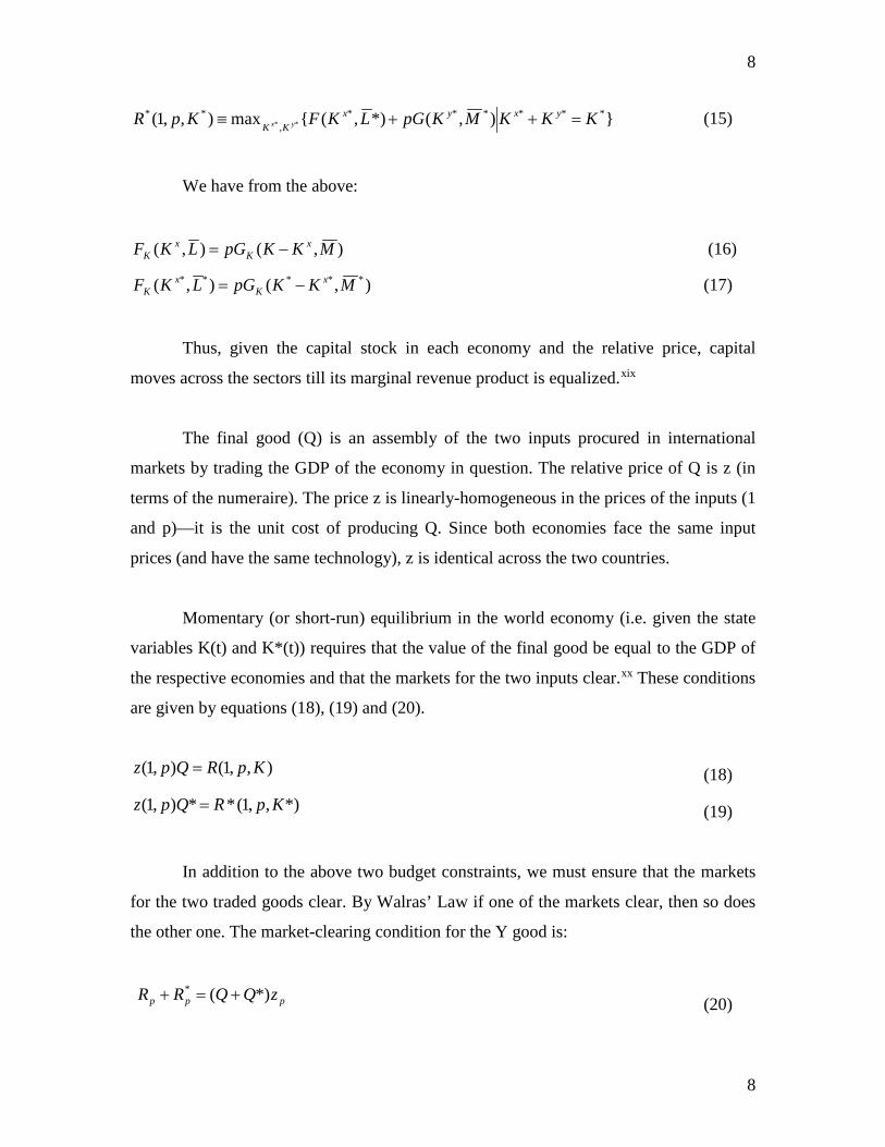
KK yx =++≡ (15)

We have from the above:

),(),( MKKpGLKF xK

xK −= (16)

),(),( ***** MKKpGLKF xK

xK −= (17)

Thus, given the capital stock in each economy and the relative price, capital

moves across the sectors till its marginal revenue product is equalized.xix

The final good (Q) is an assembly of the two inputs procured in international

markets by trading the GDP of the economy in question. The relative price of Q is z (in

terms of the numeraire). The price z is linearly-homogeneous in the prices of the inputs (1

and p)—it is the unit cost of producing Q. Since both economies face the same input

prices (and have the same technology), z is identical across the two countries.

Momentary (or short-run) equilibrium in the world economy (i.e. given the state

variables K(t) and K*(t)) requires that the value of the final good be equal to the GDP of

the respective economies and that the markets for the two inputs clear.xx These conditions

are given by equations (18), (19) and (20).

),,1(),1( KpRQpz = (18)

*),,1(**),1( KpRQpz = (19)

In addition to the above two budget constraints, we must ensure that the markets

for the two traded goods clear. By Walras’ Law if one of the markets clear, then so does

the other one. The market-clearing condition for the Y good is:

ppp zQQRR *)(* +=+ (20)

9

9

2.2 Capital Accumulation and Dynamics

The two countries have identical homothetic tastes. In particular, the rate of time

preference is identical across countries. Agents possess perfect foresight. The

representative consumer maximizes the following utility functional (a similar

specification holds for the foreign country):

∫∞

−0

)].(exp))(([ dtttCu ρ (21)

where ρ is the rate of time preference. The instantaneous utility function u(.) satisfies

𝑢𝑢′(𝐶𝐶) > 0, 𝑢𝑢′′(𝐶𝐶) < 0, 𝑢𝑢′(𝐶𝐶)𝑐𝑐→0 → ∞, and 𝑢𝑢′(𝐶𝐶)𝑐𝑐→∞ → 0.

The accumulation equations are given byxxi

)()()()( tCtKtQtK −−= δ (22a)

)(*)(*)(*)(* tCtKtQtK −−= δ (22b)

There is an initial condition on each of the capital stocks:

,)0( 0KK = (23a)

.)0( *0

* KK = (23b)

and tranversality conditions for the two economies:

,0).(exp)).((').(lim =−∞→ ttCutKt ρ (24a)

.0).(exp)).(*(').(*lim =−∞→ ttCutKt ρ (24b)

10

10

We set up the maximization problem for the representative household in the

domestic economy. The household takes the time path of p as given and maximizes the

following current-value Hamiltonian (μ is the co-state variable):

]),1(/),,1([)( CKpzpKRCu −−+≡Ω δµ (25)

The necessary optimality conditions are:

µ=)(' Cu (26)

µδρµ )/()( zRK−+= (27)

and 0).(exp)).((').(lim =−∞→ ttCutKt ρ (equation (24a) above).

Substituting (26) in (27) (and differentiating with respect to time), along the

optimal path we have the Euler equations (with )('/)('' CuCCu−≡σ )

)),()(()(/)( 1 δρσ +−= − trtCtC (28a)

Similarly for the foreign country we have:

)).()(()(/)( *1** δρσ +−= − trtCtC (28b)

Along a competitive equilibrium path, households in both countries choose

optimal paths for consumption and investment (and hence capital stocks), taking the path

of prices of factors and goods as given. Firms take the path of factor prices and goods

prices as given and maximize their profits. The resulting optimal production and

consumption decisions satisfy the market-clearing conditions.

We now turn to the steady state of the model.

11

11

2.3 The Steady State

There is a trivial steady state with 0** ==== CCKK (an overbar on an

endogenous variable denotes its steady state magnitude). The non-trivial steady state of

the model is given by setting the time derivatives in equations (22a), (22b), (28a) and

(28b) to zero. We thus have:

)(/ ρδ +=zRK (29a)

)(/* ρδ +=zRK (29b)

CKQ =−δ (29c) *** CKQ =−δ (29d)

From the properties of the GDP functions and the price indices, equations (29a)

and (29b) solve uniquely for the steady state capital stocks K and *K . Given these

equations (29c) and (29d) determine the unique values of steady state levels of C and *C . Thus the nontrivial steady state is unique.

From equation (29a) and (29b) we see that in the steady state rates of return are

equalized. From the linear homogeneity of F(.) and G(.), so are returns to L and M (these

depend only on the ratios of Kx to L and Ky to M).

We thus have:

Proposition 1: In the steady state we have factor-price equalization.

2.4 Dynamics

The behavior of the world economy over time can be represented by the four

differential equations given by (22a), (22b), (28a) and (28b).

12

12

Linearizing these four differential equations around the initial steady state and

writing in a matrix form, we have:xxii

−

−

−

−

−−−−

−−−−

=

−−

−−

**

**

**

**

**~*

**1

*~1

*~1

~1

*

*

1001

)/()/(00)/()/(00

KK

KK

CC

CC

QQQQ

ppRRzppRzppRzppRRz

KKCC

KK

KK

KKQXKKKKQX

KKQXKKQXKK

δδ

θθθθ

(30)

Or compactly:

)( VVAV −= where V≡[C, C*, K, K*]T.

0])())(([

)/)((

])/()/([.

1232

2~

***

***

2

~*

***

**2

~*

****~*

**2

>++=

++=

++=

−−

−

−

pbRRRRRz

ppRRRRRz

ppRRppRRRRzADet

QXKKKKKKKKK

KKQXKKKKKKKK

KKQXKKKKQXKKKKKK

θ

θ

θθ

(31a)

0/2/)(22. ** >=−=−+= zzRQQATr KKK ρδδ (31b)

0)2(

)/(*)/(

)]/(*)/()/(*)/([

)(

1

2**

1

**

2

**

2**

**22

<+−=

++−+−

−−+−+=

+−+−=Σ

−

−

−

×

δδ

δδ

δδ

K

Ky

Ky

yyK

yK

yKKKKKK

RzRdKdpJRdKdpJz

dKdpJdKdpJRdKdpJRdKdpJzQQQQQQ

(31c)

(In the above expressions, Jy is the import of the y-good by the home country. The value

of b32 is given in Appendix A)

13

13

Proposition 2: Matrix A has two “stable” roots and two “unstable” roots. Hence, the

long-run equilibrium is a saddle-point.

Proof: The determinant of the coefficient matrix A is positive. This implies one of

the following possibilities: (i) that there are four unstable roots i.e. with positive real parts

(if complex conjugates); (ii) four stable roots i.e. with negative real parts (if complex

conjugates); and (iii) two unstable roots (with positive real parts) and two stable (with

negative real parts). Note that the positive value of the determinant rules out the

possibility of a zero root (or hysteresis). The trace is positive, thereby ruling out all

negative roots (possibility (ii)). The sum of the product of two roots at a time (∑2×2), is

negative, so all the roots cannot be positive. We are then left with possibility (iii) i.e.,

exactly two negative roots (or with negative real parts). The steady state is therefore a

saddle-point and the stable arm is a plane. Since there are two predetermined variables (K

and K*), and two forward-looking (or “jump”) variables (C and C*), we can associate an

initial condition with each of the stable roots. The two transversality conditions rule out

explosive behavior due to unstable roots.

2.5 Steady State per Capita Income and Consumption

We showed in Proposition 1 that in the steady state there is international

equalization of the returns to all the factors of production. But what about the behavior of

consumption and investment per capita? Do these converge?

If we think of input L as labor and M as fruits (the fact fruit trees or land are

durable is discussed in the next section—here just think of M as a non-labor primary

input and look at its steady state implications). We find that differences in the endowment

of the factor of production, M, determines differences in per capita consumption. Since

the two economies are assumed different in the ratios of M/L, the economy with a higher

M/L ratio will have higher consumption and investment (equal to the depreciation of the

capital stock). Capital in the steady state is “obtainable” at a fixed price of )( ρδ +z .

14

14

Thus the economy with a higher M/L ratio will have more capital per capita so that the

ratio of capital to land in the Y sector is also equalized internationally. We have then (we

drop the overbars on M and L—these are in fixed supply throughout this paper):

)/).(/(.)/()/()/)(( LMMKgpLKfLKLCpz yx +=+δ (32)

In equation (32), f(.) and g(.) are respectively the per capita output in the X sector

and per unit of land output in the Y sector. From factor price equalization, f(.) and g(.) are

equalized internationally. Hence per capita income depends solely on the ratio M/L. We

then have:

Proposition 3: The economy with a higher per capita availability of M has higher

income, consumption and investment in the steady state.

Comment: Only if the per capita land endowment is the same across economies, is it the

case that (presumably starting from different capital stocks) will the economies converge

to identical income, consumption and investment per capita.

2.6 Behavior outside the Steady State

It is straightforward to show that the higher capital-stock economy will have a

lower rate of return to capital. The proof of this follows from the property of the GDP

function-- 0<= KKKK FR .

Why this should be so with the two economies having different endowments of

the two specific factors is not apparent at first sight. That is, in a three factor model, how

do we define a capital-poor economy? The solution lies in comparing the marginal

products in the two sectors across economies. This gives us (from equations (16) and (17)

and using linear homogeneity of F(.) and G(.)):

)/('/)/(')/('/)/(' **** MKgMKgLKfLKf yyxx = (33)

15

15

Equation (33) tells that no matter what the initial distribution of the specific factors

internationally, equalization of marginal products for the mobile factor and international

goods prices, ensures that an economy with a relatively high (low) ratio of capital

employed per worker in the X sector will also have a relatively high (low) ratio of capital

per unit of land in the Y sector.

Now it is easy to show that the capital poor economy will have a higher growth of

consumption per capita. We use the inverse relationship between the marginal product of

capital and the economy’s capital stock in equations (27) and (28) (remembering that

)/)(('))](([)( 1 LtKftpztr x−= )

))()(()(/)()(/)( *1** trtrtCtCtCtC −=− −σ (34)

Equation (33) assures us that the capital-rich country will have a lower interest

rate. Hence in (34) the capital-poor country will grow faster. We summarize this in:

Proposition 4: Outside the steady state, an economy with a lower stock of capital per

capita will have a higher interest rate and a higher growth rate of consumption per

capita compared to an economy with a higher capital stock per capita.

3. EXTENSIONS

3.1 Extension 1: Labor as the mobile factor

How does the analysis in the previous section change if instead of capital (the

factor that can be accumulated), it is labor (one of the factors in given supply) that were

mobile? This was the structure, albeit in a two period overlapping generations model, of

Eaton (1987), (1988). Suppose X is produced using labor and capital, and Y uses labor

and the other factor (M). That is:

16

16

))(),(()( tKtLFtX x= (35a)

))(),(()( tMtLLGtY x−= (35b)

In the model now,

),(),(max),,1( , LLLMLpGKLFKpR yxyxLL yx =++≡ (36)

Now the marginal product of labor is equalized across sectors;

(.)(.) LL pGF = (37)

How does the dynamic analysis change? Algebraically, it does not change very

much. In particular, conditions (31a), (31b) and (31c) are exactly the same as in the

previous case. The derivatives in Appendix A are modified, though—these are given in

Appendix B.

The dynamics of capital accumulation in either country is accompanied by labor

moving to the X sector. As this happens, an excess demand for the Y good arises that

raises p.xxiiiThis slows down the drain of labor from the Y sector.

The steady state is still given by equations (29a), (29b) and (29c) except that we

note in (31a), we have )()( ρδ +== zXR KK .

In the model of section 2, a higher land endowment calls forth higher capital

accumulation. Loosely speaking, across steady states land and capital are complements.

In the example of this section, land and capital are substitutes. A high land endowment

per capita implies a higher wage rate and a lower capital stock. This is because the rental

rate is driven down “very quickly” to its steady state value.xxiv

17

17

Note that the two cases studied so far (in Section 2 and in this sub-section)

exhaust all the possible cases of the specific factors model in a dynamic setting (this is

true as long as both L and M are inelastically supplied).

3.2 Extension 2: Durable land as a fixed factor

In this second example, let us go back to the original model, with capital being

mobile across the sectors (the analysis below holds for labor being mobile across the

sectors also). The production functions for the two goods are given by (as in section 2):

),( LKFX x=

),( MKGY y=

Now suppose M is land whose supply is inelastically given. Land is a durable

asset with a price (in terms of the numeraire) of q. Arbitrage between the return to capital

and land requires (assume land does not depreciate):

qqpYzR MK /)()( +=− δ (38a)

The return to land in (38a) consists of its marginal product and the capital gains.

Similarly for the foreign economy:

*/*)()( **

** qqpYzR MK +=− δ (38b)

Solving the differential equations in (38a) and (38b) and imposing transversality

conditions, we find that the price of land is given by the present discounted value of the

marginal product of land, where the (time-varying) discount factor is the return to capital.

18

18

∫∞

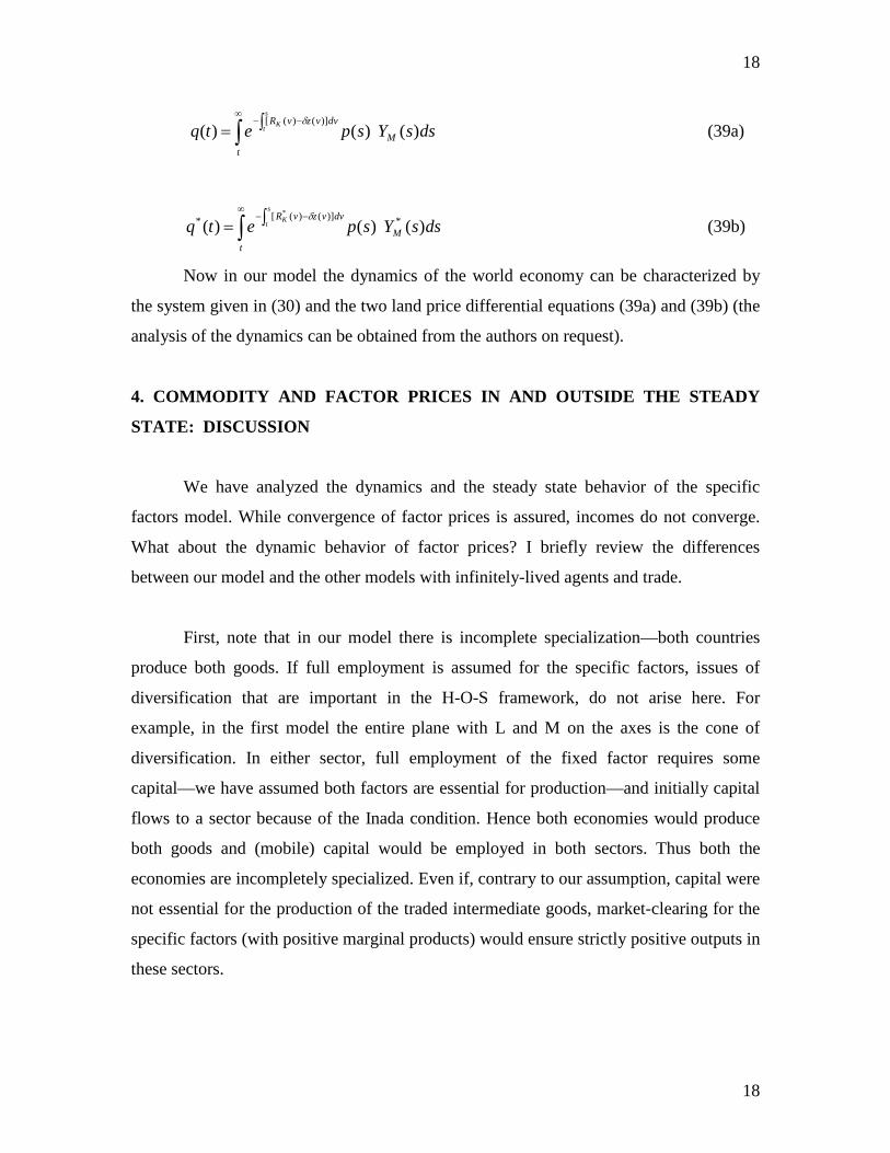
−−∫=t

M

dvvzvRdssYspetq

s

t K )()()()]()([ δ

(39a)

∫∞

−−∫=t

M

dvvzvRdssYspetq

s

t K )()()( *)]()([** δ

(39b)

Now in our model the dynamics of the world economy can be characterized by

the system given in (30) and the two land price differential equations (39a) and (39b) (the

analysis of the dynamics can be obtained from the authors on request).

4. COMMODITY AND FACTOR PRICES IN AND OUTSIDE THE STEADY

STATE: DISCUSSION

We have analyzed the dynamics and the steady state behavior of the specific

factors model. While convergence of factor prices is assured, incomes do not converge.

What about the dynamic behavior of factor prices? I briefly review the differences

between our model and the other models with infinitely-lived agents and trade.

First, note that in our model there is incomplete specialization—both countries

produce both goods. If full employment is assumed for the specific factors, issues of

diversification that are important in the H-O-S framework, do not arise here. For

example, in the first model the entire plane with L and M on the axes is the cone of

diversification. In either sector, full employment of the fixed factor requires some

capital—we have assumed both factors are essential for production—and initially capital

flows to a sector because of the Inada condition. Hence both economies would produce

both goods and (mobile) capital would be employed in both sectors. Thus both the

economies are incompletely specialized. Even if, contrary to our assumption, capital were

not essential for the production of the traded intermediate goods, market-clearing for the

specific factors (with positive marginal products) would ensure strictly positive outputs in

these sectors.

19

19

Second, international trade under competitive conditions would equalize goods

prices. In our model only the intermediate goods are traded and their prices are equalized.

In the H-O-S set up, this would imply that all factor prices are equalized in the cone of

diversification. This is because with two factors of production, in both countries, we have

(ki is the capital-labor ratio in sector i)

)('.)(' yx kgpkf = (40a)

)](')(.[)(')( yyyxxx kgkkgpkfkkf −=− (40b)

Given p, the above equations determine kx and ky and the returns to factors

depend on these capital intensities. This is the celebrated “factor-price-equalization”

result. As noted above, in a dynamic optimal growth framework this results in

hysteresis—i.e. non-convergence. A country with a higher income has the same growth

rate of consumption per capita as its poorer trading partner, implying thereby that the

initial discrepancy in consumption levels is never eliminated. In effect, trade in goods

also makes up for the lack of asset market integration.

In our dynamic specific factors model, there is (as noted above) factor price

equalization only in the steady state. The discount rate ties down the net marginal product

of capital in one of the sectors. But mobile capital across sectors ensures that the other

marginal product also gets tied down. There are two factor intensities and they are

uniquely determined by p and ρ+δ. We have (for the model of section 2):

),(),()).(,1( MKKpGLKFpz yK

xK −==+δρ (41a)

*),(*),()).(,1( *** MKKpGLKFpz yK

xK −==+δρ (41b)

Finally, a comment on the difference in the “catch-up” possibilities in this model

and the dynamic Heckscher-Ohlin model. If we think of a model with a bloc of a large

number of richer economies in steady state, and a small economy still accumulating

capital. In the example of Atkeson and Kehoe (2000), the poorer economy would

20

20

accumulate capital while completely specialized in the labor-intensive good. This

continues until it reaches the minimum capital-labor ratio of the richer bloc consistent

with factor price equalization. Its capital accumulation ceases here because the (net)

return to capital equals the rate of time preference. Thus while factor prices are equalized,

its income per capita never reaches the level of any richer country (save those that are

also the most labor-abundant among them). So a poorer economy grows richer, while the

rich remain in steady state, but they never quite catch up. In Bajona and Kehoe (2006), it

is shown that in an overlapping generations structure, economies converge to the same

capital labor-ratio. In our model (of section 2), it is possible that the richer land per capita

economy starts of being poorer in terms of income (because of a very low capital stock

initially) but then overtakes the other one before settling down as the richer economy in

steady state. Thus there is the possibility of catch-up and overtaking by the late-comer in

the specific factors model.

5. CONCLUSIONS

We showed that there is convergence (in factor prices) in a dynamic specific

factors model with two primary factors of production and without international

borrowing or lending. Only in the steady state is there equalization of factor prices. Per

capita incomes and consumptions do not get equalized if the two economies have

different endowment ratios of the primary factors per capita. Outside the steady state

there is no factor price equalization. This happens even though the economies produce

both goods. Contrast this with the H-O-S model where, incomplete specialization implies

factor-price equalization.

Our results should be seen to be suggesting that factor endowment models

generally can give sensible conclusions in a growth context. It is only in an identical-

technologies-two-factors scenario that we do not get convergence.

21

21

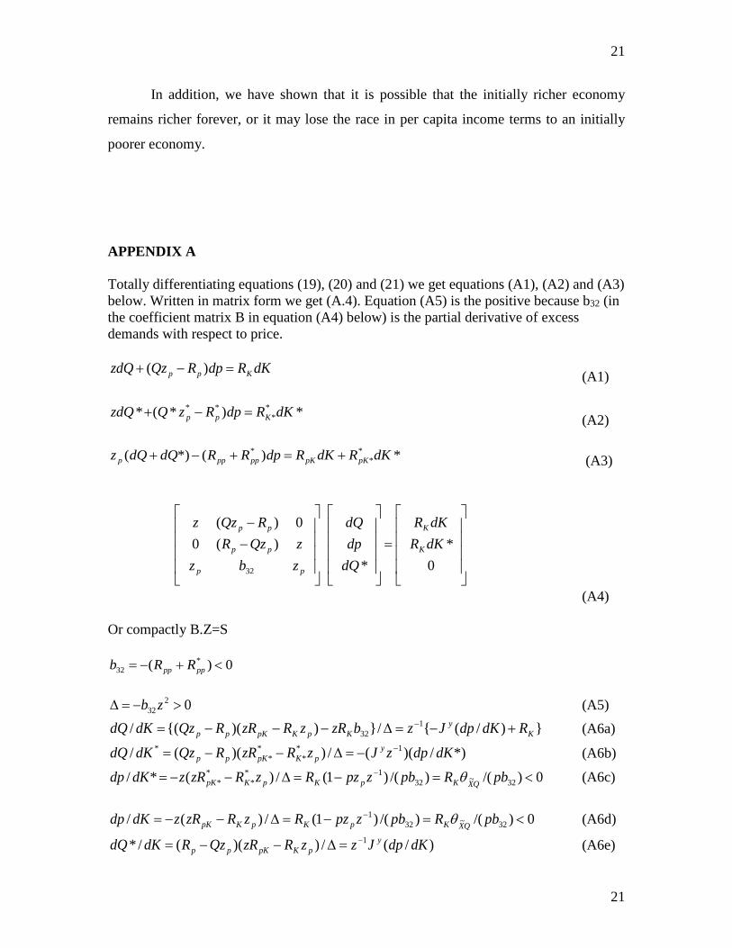
In addition, we have shown that it is possible that the initially richer economy

remains richer forever, or it may lose the race in per capita income terms to an initially

poorer economy.

APPENDIX A Totally differentiating equations (19), (20) and (21) we get equations (A1), (A2) and (A3) below. Written in matrix form we get (A.4). Equation (A5) is the positive because b32 (in the coefficient matrix B in equation (A4) below) is the partial derivative of excess demands with respect to price.

dKRdpRQzzdQ Kpp =−+ )( (A1)

*)*(* **

** dKRdpRzQzdQ Kpp =−+ (A2)

*)(*)( **

* dKRdKRdpRRdQdQz pKpKppppp +=+−+ (A3)

=

−−

0*

*)(0

0)(

32

dKRdKR

dQdpdQ

zbzzQzR

RQzz

K

K

pp

pp

pp

(A4) Or compactly B.Z=S

0)( *32 <+−= pppp RRb

02

32 >−=∆ zb (A5) )/(/))((/ 1

32 Ky

KpKpKpp RdKdpJzbzRzRzRRQzdKdQ +−=∆−−−= − (A6a)

*)/)((/))((/ 1**

**

* dKdpzJzRzRRQzdKdQ ypKpKpp

−−=∆−−= (A6b)

0)/()/()1(/)(*/ 32~321*

**

* <=−=∆−−= − pbRpbzpzRzRzRzdKdp QXKpKpKpK θ (A6c)

0)/()/()1(/)(/ 32~321 <=−=∆−−= − pbRpbzpzRzRzRzdKdp QXKpKpKpK θ (A6d)

)/(/))((/* 1 dKdpJzzRzRQzRdKdQ ypKpKpp

−=∆−−= (A6e)

22

22

*)/(/))((*/* *

*1

32*

**

**

* Ky

KpKpKpp RdKdpJzbzRzRzRRQzdKdQ +=∆−−−−= − (A6f) APPENDIX B In Appendix A, the values obtained in equations (A6a) to (A6f) are modified to:

)/(/))((/ 132 K

yKpKpp RdKdpJzbzRzRRQzdKdQ +−=∆−−−= − (B1a)

*)/)((/))((/ 1**

* dKdpzJzRRQzdKdQ ypKpp

−−=∆−−= (B1b)

0/)(*/ ** >∆= pK zRzdKdp (B1c)

0/)(/ >∆= pK zRzdKdp (B1d)

)/(/))((/* 1 dKdpJzzRQzRdKdQ ypKpp

−=∆−−= (B1e)

*)/(/))((*/* **

132

**

** K

yKpKpp RdKdpJzazRzRRQzdKdQ +=∆−−= − (B1f)

REFERENCES Atkeson, Anthony, and Patrick J. Kehoe (2000) “Paths of Development for Early- and

Late-boomers in a Dynamic Heckscher-Ohlin Model,” Research Staff Report No. 256,

Federal Reserve Bank of Minneapolis.

Arnold, Lutz G. and Stefanie Trepl (2015) “A North-South Trade Model of Offshoring

and Unemployment,” Open Economies Review 265, 999-1039.

Bajona, Claustre and Timothy J. Kehoe (2006) “Demographics in Dynamic Heckscher-

Ohlin Models: Overlapping Generations versus Infinitely Lived Consumer,” Research

Staff Report No. 377, Federal Reserve Bank of Minneapolis.

---------(2010) “Trade, Growth, and Convergence in a Dynamic Heckscher-Ohlin

Model,” Review of Economic Dynamics 13, 487-513.

Barro, Robert J. and Xavier Sala-i-Martin (2003) Economic Growth, Second Edition,

MIT Press.

Baxter, Marianne. (1992), “Fiscal Policy, Specialization, and Trade in the Two-sector

Model: The Return of Ricardo?” Journal of Political Economy 100, 713–44.

23

23

Bianconi, Marcelo, (1995) “On Dynamic Real Trade Models”, Economics Letters, 47,

47-52.

Brecher, Richard A., Zhiqi Chen, and Ehsan U. Choudhri (2002) “Absolute and

Comparative Advantage, Reconsidered: The Pattern of International Trade with Optimal

Saving” Review of International Economics, 10, 645–656.

Brock, Phillip.L. and Stephen. J. Turnovsky, (1993) “The Growth and Welfare

Consequences of Differential Tariffs”, International Economic Review 34, 765–794.

Caliendo, L (2009) “On the Dynamics of the Heckscher-Ohlin Theory”, Department of

Economics, University of Chicago.

Chatterjee, P. and M. Shukayev (2012) “A Stochastic Dynamic of Trade and Growth:

Convergence and Diversification”, Journal of Economic Dynamics & Control 36 416–

432.

Chen, Zhiqi (1992) “Long-run Equilibria in a Dynamic Heckscher-Ohlin Model”

Canadian Journal of Economics 23, 923–43.

Davis, Donald R. and David E. Weinstein (1998) “An Account of Global Trade,” NBER

Working Paper 6785.

Dixit, Avinash and Victor Norman (1980), Theory of International Trade: A Dual,

General Equilibrium Approach, Cambridge, MA: Cambridge University Press.

Eaton, Jonathan (1987) “A Dynamic Specific-Factors Model of International Trade”,

Review of Economic Studies, 54, 325-338.

----------------------(1988) “Foreign-Owned Land”, American Economic Review, 78, 76-88.

Fedotenkov, Igor, Bas van Groezen and Lex Meijdam (2014) “Demographic Change,

International Trade and Capital Flows,” Open Economies Review 25, 865-883.

Harrigan, James, (1997) “Technology, Factor Supplies and International Specialization:

Estimating the Neoclassical Model,” American Economic Review 87, 475–94.

Hu, Yunfang, Kazuo Nishimura, and Koji Shimomura (2006) “Dynamic Three Factor

Models of International Trade” Asia-Pacific Journal of Accounting and Economics 13,

73-85.

24

24

-----------(2008) “Specific Factor Models and Dynamics in International Trade,” in

Sugata Marjit and Eden S. H. Yu (eds) Contemporary and Emerging Issues in Trade

Theory and Policy (Emerald Publishers, Bingley, UK), 191-207.

Komiya, Ryutaro, (1967) “Non-Traded Goods and the Pure Theory of International

Trade,” International Economic Review 8, 132–52.

Jones, Ronald W. (1971) “A Three-Sector Model in Theory, Trade, and History,” in

Bhagwati, J.N., R.W. Jones and J. Vanek (eds.) Trade, Balance of Payments and Growth,

(North-Holland Publishing Company, Amsterdam).

Joseph, Francois, and Clinton R. Shiells (2008) “Dynamic Factor Price Equalization and

International Convergence” Johannes Kepler University of Linz, Working Paper No.

0820.

Kaneko, A. (2006) “Specialization in a Dynamic Trade Model”, International Economic

Journal 20, 357-368.

Laitner, John (2000) “Structural Change and Economic Growth” Review of Economic

Studies 67, 545-561.

Mountford, A. (1998) “Trade, Convergence and Overtaking”, Journal of International

Economics 46, 167-182.

Neary, Peter, 1978, “Short-Run Capital Specificity and the Pure Theory of International

Trade”, Economic Journal 88, 488–512.

Oniki, Hajime, and Hirofumi Uzawa (1965), “Patterns of Trade and Investment in a

Dynamic Model of International Trade,” Review of Economic Studies 32, 15–38.

Sen, Partha (2013) “Capital Accumulation and Convergence in a Small Open Economy”

Review of International Economics 24, 690-704.

---------------(2015) “Uncertain Lifetimes and Convergence in a Two-country Heckscher-

Ohlin Model” Mathematical Social Sciences 78, 14-20.

Stiglitz, Joseph E. (1970) “Factor Price Equalization in a Dynamic Economy” Journal of

Political Economy 78, 456–88.

25

25

Tadesse, Bedassa and Roger White (2010) “Does Cultural Distance Hinder Trade in

Goods? A Comparative Study of Nine OECD Member Nations,” Open Economies

Review 21, 237-261.

Trefler, Daniel, (1993) "International Factor Prices: Leontief Was Right!" Journal of

Political Economy 111, 961-87.

———(1995) “The Case of Missing Trade and Other Mysteries,” American Economic

Review 85, 1029–46.

Ventura, Jaime (1997) “Growth and Interdependence,” Quarterly Journal of Economics

112, 57–84.

Woodland, Alan (1982) International Trade and Resource Allocation, (Amsterdam)

North Holland.

i The world economy, of course, is a closed economy and hence a decline in the return to capital accompanies any accumulation of capital. ii It is not even a candidate to explain trade between similar economies or intra-industry trade. iii See Bardhan (1965), Oniki and Uzawa (1965) and Stiglitz (1970) for early contributions with saving being a constant proportion of income. Stiglitz (1970) also considers optimal savings but with the rate of time preference differing between economies. Woodland (1982) uses duality and sketches a dynamic model. iv For a discussion of finite lives in dynamic trade models, see e.g. Bajona and Kehoe (2006—who have a many-period overlapping generations models, (they also discuss capital flows), Bianconi (1995) who has a two period overlapping generations structure and Kaneko (2006) with a continuous time uncertain lifetimes structure. v Below we will see that tampering with this assumption (of only two factors that are mobile across the two sectors) that will result in very different predictions. vi If labor supply is elastic, as e.g. in Chen (1992) then factor price equalization also equalizes the marginal utility of leisure. vii This relies on the evidence on the factor content of trade (Trefler (1993), (1995), Davis and Weinstein (1998)) and on the pattern of production (Harrigan (1997)). viii The case of uniform Hicks-neutral superiority has received some empirical support from Trefler (1995) and Davis and Weinstein (1998). ix For the US, all private land constituted 31 percent of total wealth in 1900 and 16 percent in 1958. For the UK, it was 55 percent in 1798, 18 percent in 1885 and 4 percent in 1927. These figures are taken from Laitner (2000). x A small open economy model is discussed in Sen (2013). In a small open economy model factor-price equalization follows—in our two-country model, this happens only in the steady state.

26

26

xi See Arnold and Tepl (2015), Fedotenkov, van Groezen and Meijdam (2014), and Tadesse and White (2010). xii Thus there is no need to identify one of the specific factors as land and other as labor, as is done below. I do this to fix ideas. Later on (in section 3) I give other interpretations. Clearly, the framework is richer than the limited interpretations given in this paper. xiii Chen (1992) and Atkeson and Kehoe (2000) are examples. A previous version of our paper used this specification. xiv Ventura (1997), Chaterjee and Shukayev (2012) and Francois and Shiells (2008) use this structure. Atkeson and Kehoe (2000) discuss this briefly. xv See Brecher, Chen and Choudhri (2002) and Bajona and Kehoe ((2006), (2010)) for this structure. xvi The specific factors L and M could be thought of as two kinds of labor. The interpretation that suits the analysis in section 2 is to think of L as labor and M as some endowment of fruits. In section 3.2, we introduce the valuation of the trees that bear these fruits (as in Eaton (1987), (1988)). In the earlier dynamic specific factors models, the capitals in the sectors were specific in the short run, while labor was mobile across sectors (Neary (1978)). In the long run, capital was also mobile across sectors, and the model collapsed into the familiar Heckscher-Ohlin model. xvii Where there is no chance of confusion, we do not explicitly write the time index. xviii Constant growth rates for L and M can easily be incorporated, as can exogenous technical progress. xix Note, while it would be interesting to look at an internationally mobile factor whose return is equalized internationally, such an assumption with free trade in the two intermediates and constant returns to scale would make all factor prices determined internationally. It would be possible to pursue this with one intermediate being non-traded and/or decreasing returns to scale technologies. xx This is essentially reproducing the analysis of Dixit and Norman (1980), chapter 5. xxi Since there is no borrowing or lending internationally, capital is the only store of value. If one of the specific factors was, say, land, then savings would also be allocated to a change in the value of land—see section 3.2 below. In an overlapping context, this can be crucial (see Eaton (1987), (1988)). xxii We are going to use the relationships given in the Appendix A. xxiii Since capital is now used exclusively in the X sector, its accumulation causes the supply of the Y good to fall, causing excess demand for the latter good and its price to rise. This is the big difference in the details of this example over the set-up where capital was the mobile factor. Note that this does not change the stability of the model, or its (qualitative) dynamics. xxiv The issue of land availability on the development path of a small open economy is discussed in Sen (2013).