In this course on time series analysis we will

discuss the properties of the analysis of data

that are ordered in time.

Any given data point can to first order be

characterized as containing three values;

time, signal and noise.

An example of a 5 day time series of the

integrated velocity signal of the solar surface.

The time series contains long and short term

noise and periodic oscillations.

A zoom of 5 hours of the above time series. One

clearly see the oscillations.

A 30 min. zoom. Oscillations can be seen,

however it is also clear that the data contain

noise.

Due to noise (and due to the non-stable

behaviour of the solar oscillations concerning

frequency, amplitude and phase) the measured

properties of a given oscillation will contain

errors. Those errors depend on the properties of

both the signal and the noise. In order to

understand the quality of a parameter for an

oscillation one will need to understand the

properties of the noise.

Noise is therefore as important to consider as

the signal is.

We may begin by considering the simple

parameters for a time series (relevant not only

for the noise but also for the signal);

Mean, variance and standard deviation

Also the sample skewness is an important

parameter to calculate in order to characterize

the properties of a time series.

Finally the distribution functions will also contain

important information in order to understand the

properties of a given oscillation.

In time series analysis one will often assume (or

approximate) the different noise sources to be a

simple noise source having a Normal (or

Gaussian) distribution. We will later in the

course learn that this is certainly not always an

appropriate assumption and one may introduce

large errors in estimating the significance of a

given oscillation if one assume Normal

distributed noise for all noise sources in a given

time series.

In this figure we show a simple Normal

distributed noise source with zero mean and

standard deviation (often also called the spread

or the scatter) equal to one. The sample

skewness is zero (the distribution is

symmetrical).

The corresponding cumulative distribution

function (not normalized on the x-avis) is seen in

this figure.

Finally we show the probability function for the

distribution (observed and theoretical – based

on knowledge on the Normal distribution).

If we now compare this time series (the normal

distribution) with a time series….

that show a strong Skewness (-1 in this case)

one can directly from the time series see the

difference (that is also evident from the

skewness value).

The cumulative distribution function for this time

series is seen here…

Here the probability density function (that clearly

show the asymmetrical properties of the present

time series) is shown.

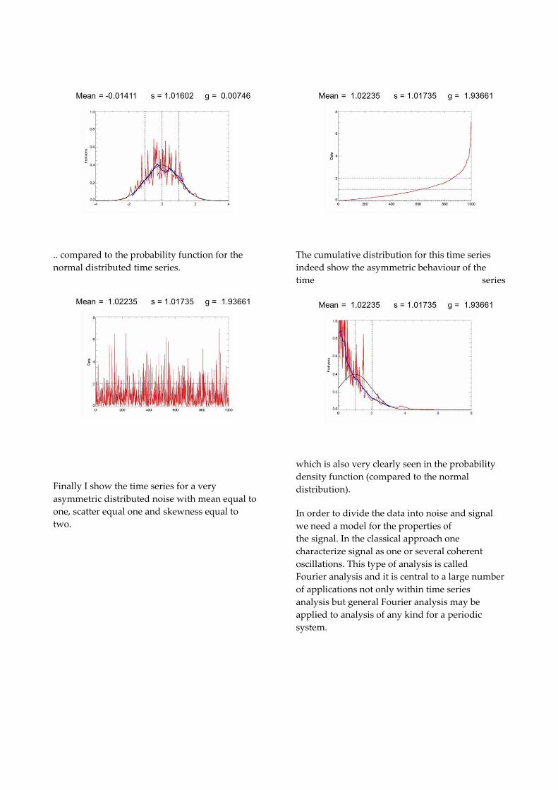
.. compared to the probability function for the

normal distributed time series.

Finally I show the time series for a very

asymmetric distributed noise with mean equal to

one, scatter equal one and skewness equal to

two.

The cumulative distribution for this time series

indeed show the asymmetric behaviour of the

time series

which is also very clearly seen in the probability

density function (compared to the normal

distribution).

In order to divide the data into noise and signal

we need a model for the properties of

the signal. In the classical approach one

characterize signal as one or several coherent

oscillations. This type of analysis is called

Fourier analysis and it is central to a large number

of applications not only within time series

analysis but general Fourier analysis may be

applied to analysis of any kind for a periodic

system.

In time series analysis the signal in the Fourier

Analysis is described by a simple harmonic

oscillator. In this equation ω0 is the angular

frequency that related to the cyclic frequency (ν)

via ω=2π·ν. The period of the oscillation is 1/ν

In the article by Jørgen Christensen-Dalsgaard;

Lecture Notes on Stellar Oscillations the Fourier

transform is analysed analytically and it is

shown that the Fourier transform of a simple

harmonic oscillator gives rise to two so-called

Sinc-peaks at frequency ω and –ω.

The sinc-function

The power spectrum is defined as the square of

the norm of the Fourier transform.

It can be shown (which will not be done here)

that the power for a given time series at

frequency f is identical to the sum of the square

of the sine- and cosine-weighted means of the

data.

If we use this formulation of the power spectrum

we are able to calculate the power spectrum of

a simple harmonic oscillator as follows.. which

will be our recipe for calculating power spectra

for time series data.

In red we show the simple harmonic oscillator.

If we now take a frequency ν and want to

calculate the power of the simple harmonic

oscillator at that frequency we shall now weight

the simple harmonic oscillator with sine and

cosine for that frequency.

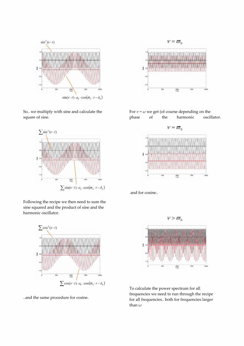
So.. we multiply with sine and calculate the

square of sine.

Following the recipe we then need to sum the

sine squared and the product of sine and the

harmonic oscillator.

..and the same procedure for cosine.

For ν = ω we get (of course depending on the

phase of the harmonic oscillator.

and for cosine..

To calculate the power spectrum for all

frequencies we need to run through the recipe

for all frequencies.. both for frequencies larger

than ω

… and for frequencies smaller than ω

Following the recipe we will now calculate the

sine-weighted mean for all frequencies…

and the cosine-weighted means…

Square them…

and calculate the sum. This is the power

spectrum of the simple harmonic oscillator.

The power spectrum shows this characteristic

structure. In this plot we show the amplitude

spectrum (the square root of the power)

If we show the power spectrum for the single

harmonic oscillator at a broader frequency

range we find the full sinc-function.

SInc is the product of 1/x and sin(x).

The power spectrum of a single harmonic

oscillator is also called the window-function.

We will discuss this in more detail during the

course.

..

.. so this is the recipe for calculating the power

spectrum.

The power spectrum and the amplitude

spectrum are related such that the power is the

square of the amplitude.

In order to understand why Fourier analysis is

such a powerful tool for time series analysis, we

need to consider the power spectrum for a noise

source.

We will first consider a Normal distributed noise

source.

For such a noise source we known from

statistics that the are relations between the

noise characteristics and the mean, variance..

.. in fact one thing we know is that the scatter on

the measurement of the mean is given by:

σ(μ)² = σ²/N

From calculating the sine- and cosine-weighted

mean values we then find..

So, the level of a noise source will decrease

with number of data points.