1

In this chapter we discuss the production of electromagnetic waves. The real trick here is to develop techniques that allow us to compute closed form solutions for the electric and magnetic field as opposed to series expansions similar to approach we used towards the end of Physics 435. For example, in one of the problems in the last homework, you had an oscillating solenoid, that would create a Faraday electrical field, that would create a correction to the magnetic field due to the displacement current that would modify the Faraday electric field etc. There is a lot of fascinating physics here. We begin with production of plane polarized waves from an oscillating, infinite current sheet. Here we are able to solve for the fields and radiated energy by matching the B field from the plane polarized waves to the B-field generated by the Ampere term of current sheet since we can show that displacement contribution is negligible. The usual way that radiation problems are handled in closed form is through the potential formulation where we use “retarded” versions of the same scalar and vector potential integrals developed in Phys435. These retarded potentials imply that if one turns on a current, a far away observer doesn’t immediately see an Ampere’s law B-field but must wait for the “information” to get there. Interestingly enough the information travels at the speed of light. We are able to get a simple, closed form solution for this problem, We then switch to radiation from oscillating antennae and work out the electromagnetic fields, the Poynting vector and the total radiated power. We next consider the electromagnetic fields produced by a moving and possibly accelerating charge. The retarded potentials for a moving charge, called the Lienard-Weichert potentials, were developed around 1900. We conclude with an application of the Lienard-Weichert potentials by considering “synchrotron” radiation from very relativistic electrons stored in a circular accelerator. Interestingly enough, although the electrons are ultra-relativistic, we can successfully compute synchrotron radiation using classical electrodynamics. The classical theory is automatically consistent with special relativity and in fact was Einstein’s inspiration.

2

We begin with perhaps the simplest radiation example: the radiation of an infinite, oscillating current sheet. The reason this problem is very simple is that one essentially gets the B-field from the classical Amperian loop that we used to get the B-field from a static current sheet in Physics 212. If we restrict our self to the region just outside the sheet, and assume finite electric fields, we can ignore the contribution due to the Maxwell displacement current since this component is proportional to the area of the Amperian loop which approaches zero. Once we are outside of the current sheet, we have the propagation of plane electromagnetic waves in a vacuum since there is no charge or current outside of the plane. For waves in a vacuum we know the waves propagate in a direction perpendicular to the B-field which is aligned along the y direction from our Amperian construction which means it must propagate in either the +/- z or +/- x direction. But the current is uniform in x and thus the field cannot have an x dependence which restricts us to +/- z propagation or waves that either approach or recede from the current sheet as shown in the figure. The case where the wave’s propagate toward the current sheet doesn’t make sense if we think about starting the oscillation at time t=0. If the waves are moving away from the current sheet, they get to a far away point at a time t > 0 and all is fine since the future electric field depends on the past. On the other hand, if the waves are moving towards the current sheet, the waves must be traveling at t<0 so that they can arrive at the current sheet at t=0. The waves evidently start traveling before they are created. Essentially a wave that appears in the present, was created in the future! It is as if the incoming wave anticipated the start of the current oscillation so that it could travel to the current plane and match the oscillation source. We say that the case where the waves propagate into the sheet violates causality. This is a “philosophical” boundary condition – we cannot get it from the wave equation alone which is symmetric in t -t. We can then match the B-fields from two waves that radiate outwards from the current sheet to the fields due to the Amperian construction and find the associated E-field from Faraday’s law. We find that the electrical field oscillates in the +/- x-hat direction which in the direction of the current flow. The maximal electrical field is typically along or against the direction of the current in radiation problems. Here it is only parallel to +/- direction of the current since we have perfect plane polarized electromagnetic waves. Magnetic field is perpendicular to the electric field, down by a factor of c and in a direction such that E cross B is in the direction of propagation. Technically our solutions are only valid a long time after the currents start oscillating. As we will see, immediately after the “information” arrives there are typically large transients which damp out leaving the indicated steady state solutions.

3

Since we now know the electric and magnetic field, we can compute the intensity or time-averaged Poynting vector. Not surprising it lies in the direction of propagation – away from and perpendicular to the current sheet – and is a very simple expression proportional to the square of the amplitude of the surface current. The most practical way of handling the general radiation problem is to use the vector and scalar potential. As we will show shortly, we can get relatively simple integral expressions for the potentials which will allow us to solve for the electric and magnetic fields as derivatives of the potentials rather than through the series method we discussed at the end of Physics 435 where the we would solve for say the electric field in an oscillating capacitor, which would create an oscillating magnetic field from the displacement current, which in turn would create a correction to the electrical field through Faraday’s law etc. The potential approach leads to “closed” form integral solutions. It is still possible to define a vector potential for the magnetic field where B is the curl of A even in electrodynamics. Since if B is the curl of A, the gradient of B must vanish but divergence of B is always zero even after Faraday’s law and the addition of displacement current contribution to Ampere’s law. However we cannot write the electrical field as the negative gradient of a scalar potential since this would imply that the curl of the E-field must vanish. But the curl of E does not vanish in electrodynamics since by Faraday’s law it is proportional to the rate of change of B. However, we can construct a curl-less field as E + partial A/partial t and set this equal to the negative gradient of V. We thus have a fairly simple extension of E being the gradient of V. E is the negative gradient of V minus the time derivative of A. We can get the equation for the A and V potentials by inserting our E and B expressions in terms of potential into the two Maxwell equations that involve the electromagnetic sources rho and J. The two expressions are fairly complicated and A is badly coupled with V.

4

We can use Gauge invariance to massively simplify the A and V source expressions. Gauge invariance allows us to define A such that the annoying divergence of A plus the time derivative of V/c^2 term equals zero by adding the divergence of a suitable function of time and space which we call Lambda. Recall we can always add the divergence of a function to A to produce a new A’ vector potential with the same B-field since the curl of a divergence always vanishes. In order to produce the same E field with the new A’, we must also compensate the potential with the negative time derivative of our gauge function Lambda. It isn’t obvious that one can always find a Lambda such that the annoying Del dot A + (partial V/partial t)/c^2 term vanishes but we can show that Lambda essentially satisfies a “sound wave” equation with a source proportional to the original annoying term and such a solution always exists. The gauge which kills the annoying term is called the Lorentz Gauge. The Coulomb Gauge, used for static fields, is essentially the same as the Lorentz Gauge for “static” voltages. The Lorentz Gauge not only kills off the annoying term, but simultaneously decouples the V and A expressions. In both cases, an “d’Alembertian” operator consisting of time and space derivatives acts on A or V to give the source of A and V (namely J and rho). This is a truly beautiful result that presages special relativity. The d’Alembertian operator puts time and space derivatives on an equal footing. We will learn shortly that they form a “4-vector” with the time and space combined to form a 4 dimensional space-time. The charge and current densities can be combined into a 4-vector as well and finally the scalar and vector potentials form yet again another 4-vector. The extra factors of c to insure that all components of the four vector have the same dimensions. We will learn that these 4-vectors are much more than a convenient grouping of 4 related objects but rather describe how the 4 components get mixed up by a moving observer – in much the same way as a rotation mixes up the components of a 3-vector.

5

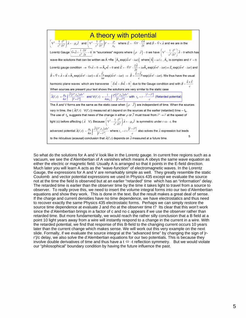
So what do the solutions for A and V look like in the Lorentz gauge. In current free regions such as a vacuum, we see the d’Alembertian of A vanishes which means A obeys the same wave equation as either the electric or magnetic field. Usually A is arranged so that it points in the E-field direction. Much later you will learn A acts as the “wave-function” of electromagnetic waves. In the Lorentz Gauge, the expressions for A and V are remarkably simple as well. They greatly resemble the static Coulomb and vector potential expressions we used in Physics 435 except we evaluate the source not at the time the field is observed but at an earlier “retarded” time which has an “information” delay. The retarded time is earlier than the observer time by the time it takes light to travel from a source to observer. To really prove this, we need to insert the volume integral forms into our two d’Alembertianequations and show they work. This is done in the text. But the result makes a great deal of sense. If the charge and current densities have no time dependence, we have electrostatics and thus need to recover exactly the same Physics 435 electrostatic forms. Perhaps we can simply restore the source time dependence at evaluate J and rho at the observer time t? Its clear that this won’t work since the d’Alembertian brings in a factor of c and no c appears if we use the observer rather than retarded time. But more fundamentally, we would reach the rather silly conclusion that a B field at a point 10 light years away from a wire will instantly respond to a change in the current in a wire. With the retarded potential, we find that response of this B-field to the changing current occurs 10 years later than the current change which makes sense. We will work out this very example on the next slide. Formally, if we evaluate the source integral at the “advanced time” by changing the sign of |r-r’|/c delay, we also solve the d’Alembertian equations for our two potentials. This is because they involve double derivatives of time and thus have a t -t reflection symmetry. But we would violate our “philosophical” boundary condition by having the future influence the past.

6

As a simple first example, we consider the B-field from an infinite wire observed at transverse distance of s from the wire. We apply a constant current starting at t=0. We only need to consider the vector potential since we assume the wire is neutral , (rho = 0 at all times). Our first step is to replace the A volume integral by a line integral over the current evaluated at the retarded time. But the retarded time depends on the observer time as well as z’ and s. We only get a non-zero current I_0 if t_R> 0 which sets limits on the z’ values that contribute to the A integral. The electrical field is easy to evaluate since it involves the time derivative of A and t only appears in the integration limit so we can use Leibnitz rule. This is a version of fundamental theorem of calculus which only involves simple derivatives. Since B is the curl of A, the simplest approach is to do the integral. The resulting indefinite integral is known and we get a simple closed form expression for the vector potential. We will get an unphysical complex component to A unless the quantity under the radical is positive which implies we will only have a non-zero A for times greater than s/c. This makes a great deal of sense since if the source is 10 light-years away, the information that we turned the current on must travel the s=10 light years to get to the observer and hence the observer first senses the B-field 10 years later! We can differentiate the A-expression with respect to time and space to get relatively simple E and B field expressions which both turn on at t_0=s/c. At long times compared to t_0 the B-field becomes the magnetostatic field given by Ampere’s law and the E-field disappears. The vanishing of the E-field at long times makes a great deal of sense since there is no charge and the Faraday contribution which is proportional to dB/dt vanishes as the B-field becomes static. The somewhat surprising result is that both the E-field and B-field become infinite at t_0 when the “information” is first received after 10 years. I think this is because we are assuming an infinitely sharp current turn on at t=0. This means that B goes from 0 to non-zero immediately at t_0 which implies an infinite dB/dt. We thus get an infinite magnetic flux derivative which induces an infinite E. The transition from E=0 to infinite E at t_0 implies an infinite displacement current which in turn creates an infinite B contribution. The “transient” behavior when the “signal” is first received is pretty dramatic and worth the 10 year wait!

7

We can also check our previous calculations (slide 2) of the oscillating current sheet using the retarded potential. We use the surface form since we are using K rather than J. We put the observer on the z axis and the source on the plane at location s’ shat’. This means the Griffiths relative displacement is sqrt(s^2 + s’^2). We first use the relative displacement to evaluate the surface current at the retarded time. We also need it to calculate the 1/r term in the vector potential integral. Our area integral involves 2 pi s’ ds’ with s’ from 0 to infinity. We evaluate this integral using a similar nu substitution as we used to evaluate the magnetostatic current plane and end up with a very simple integral over nu which leads to a very simple A expression involving the cos (omega t - k|z|) from the lower limit and cos (infinity) from the upper limit. The same cos (infinity) problem occurred in the calculation of the vector potential of magnetostatic current plane that we worked out in Physics 435. Essentially we treat it as a constant which has no effect on the E or B field since they involve derivatives of the vector potential. We next compute the E-field by taking the negative time derivative of the vector potential. We write the omega t – k|z| argument as omega t – k z for z >0 and omega t + k z for z<0. We get the same electrical fields as on slide 2. The electrical field corresponds to waves traveling in the + or – z direction away from the current plane. Interestingly enough, if we use the advanced potential rather than the retarded potential integral, we would get the same acausialsolutions (in red) of waves coming from infinity towards the current plane.An alternative method (not used here) to find E is to integrate over a new variable nu= w t – k|z|. One can then find E using Leibnitz rule to find the time differential of A-vec.

8

We turn next to a much more prosaic example of radio waves from a dipole antenna. We model the antenna by a “complex” sinusoidal charge induced in two metal spheres at the ends of the antenna. Our observer will be a distance r+ from the + pole of the dipole and r- from the – pole of the dipole. Since we just have two points, our volume integral becomes a sum over the charge at the two poles. The only electrodynamic adjustment is to evaluate the exp(i omega t) at the retarded time rather than the observer time. We assume d is small on the scale of observer distance and thus approaches an ideal dipole. The dipole approximation allows us to write r+ and r- in terms of the observer distance to the center of the antenna, the antenna length d, and the angle of the observer relative to the antenna. We can get the r+ and r- expression from the illustrated triangle in the long distance limit where r+ , r, and r- are nearly parallel. Writing the sinusoidal oscillation in complex form allows us to very easily write the potential as an oscillation factor [exp(i omega t- k r)] times a geometry factor involving r,dand theta. This geometry factor involves the difference of two terms where d <=> -d going from the first to second term. Since d is small compared to lambda, kd << 1 where (k=2pi/lambda) and we can expand the geometry exponential expression about kd keeping only the lowest order terms. We are left with a constant term (i) – implying the potential is 90 degrees out of phase with the oscillation and a term which falls as 1/kr. If we further assume the observer is very far away on the scale of the wavelength, we can drop the second term. The requirement that r >> lambda is called the radiation zone or far field limit. The near field limit can also be calculated and for this case we essentially get the quasi-static result for an oscillating dipole (exactly the same as the Physics 435 dipole except it oscillates). The near field form is pretty inevitable since as omega => 0 we go to a static dipole. The 1st term dies off as 1/r which is much slower than the second 1/r^2 term and thus is the term responsible for radio communication. The practical limit is thus the far field limit or radiation zone. As we will see later, this implies that the far zone total radiated power is constant as a function of radius.

9

We can easily recast our V expression in this case in terms of the dipole moment amplitude or p_0 vec = d q_0 z-hat. In order to get the E and B fields we need to know A as well. This involves a line integral of the current evaluated at the retarded time. We use a simple model for the current as the time derivative of q at the two pole balls on either end of the antenna. Interestingly enough, the current entering the top ball equals the current exiting the lower ball and we can model it as a uniform, oscillating current over the antenna length . The continuity equation tells us the uniform current is consistent with our charge model says there is no charge build up except at the antenna end balls thus giving us a dipole antenna. Assuming d is small compared to r and k , the exp(-i k r) can be safely taken out of the current integral leading to a very simple expression for A which is proportional to qd or p_0 as well. We take the curl of A in the far field limit using a trick.If kr >> 1, the derivatives of e-tilde are much larger than the derivatives of all other terms such as 1/(4 pi r). We can thus replace a rather tedious curl by the gradient of e-tilde, ignoring all other position dependences in the curl. We get a B-field in the phi direction in the far field limit much quicker than the full curl calculation done in the text. We compute the E-field by taking the divergence of the scalar potential (using the same gradient e-tilde trick) and the time derivative of the vector potential. The time derivative of the A has an r-hat component which is canceled by the gradient of the scalar potential leaving an E-field with only a theta component. As is the usual situation , the electrical field is perpendicular to and larger than the magnetic field by a factor of c.

10

Both E and B carry a exp(i omega t – ik r) modulation very much like a plane wave. Both E and B are proportional to sin(theta) and fall as 1/r. This means the Poynting vector is in the theta-hat cross phi-hat direction which puts it in the r-hat direction. Hence the waves radiate energy from the center of the antenna with intensities that fall as 1/r^2 and are proportional to sin(theta)^2 and the square of the dipole moment amplitude. This means the most of the power is transmitted in the plane transverse to the antenna in sort of a donut pattern. Since E is polarized along the theta direction, the maximum power is radiated with the electrical field oscillating along or against the antenna direction which is along or against the antenna current. There is an interesting theorem called antenna reciprocity which says that the configuration for maximum antenna radiation is the same as the maximum configuration for maximum antenna reception. Hence the best way to receive the signal is to put an antenna in the x-y plane orientated in the maximum E-field direction which is parallel to sending antenna direction. We can get the total radiated power by integrating the Poynting vector over the area of a sphere centered at the antenna center taking into account of the sin^2 (theta) factor. We get the same power passing through the sphere independent of the radius (since <S> propto 1/r^2) and we would presumably would get the same power passing through a near field sphere although our calculation assumed we are in the far field. The radiated power is proportional to the square of the dipole amplitude and 1/(wave length)^4. The wavelength dependence and the reciprocity theorem, explains why the midday sky is blue and the setting sun is red. The skylight is due to light scattering from air molecules acting as antenna with absorb and radiate at shorter (blue wavelengths). The blue components of the light from the setting sun are primarily scattered leaving the a transmitted red component.Another important electromagnetic source is magnetic dipole radiation. Here we pass a sinusoidal current through a small wire loop of radius b. Presumably the loop is electrically neutral so we only need to consider the vector potential. We essentially have the same integral expression and expansion technique that we used to compute A for a small static loop in one of the Physics 435 homework problems. The only difference is that we need to use an oscillating current evaluated at the retarded time. We are left with the integral over a circular path of exp(-i k |r-r’|)/|r-r’| where r is the observation point and r’ is a source point on the loop. We can write the path element as b dphi times the phi-hat unit vector. Our only job is to expand exp(-i k |r-r’|)/|r-r’| in the small coil limit using essentially the same approach used in the old homework problem. We begin by expanding |r –r’| to 1st order in b. The leading term is r and the correction terms are x/r and y/r times sin(phi) and cos(phi). Here the observer is at (x,y,z).

11

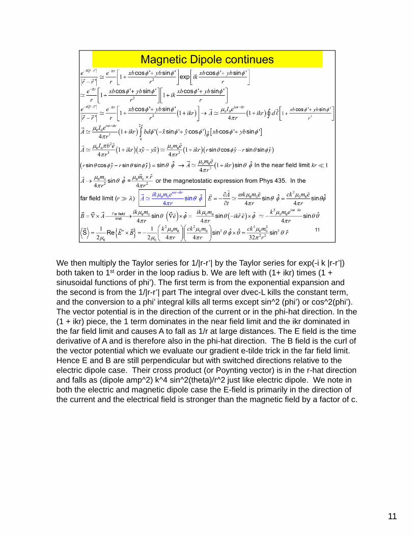
We then multiply the Taylor series for 1/|r-r’| by the Taylor series for exp(-i k |r-r’|) both taken to 1st order in the loop radius b. We are left with (1+ ikr) times (1 + sinusoidal functions of phi’). The first term is from the exponential expansion and the second is from the 1/|r-r’| part The integral over dvec-L kills the constant term, and the conversion to a phi’ integral kills all terms except sin^2 (phi’) or cos^2(phi’). The vector potential is in the direction of the current or in the phi-hat direction. In the (1 + ikr) piece, the 1 term dominates in the near field limit and the ikr dominated in the far field limit and causes A to fall as 1/r at large distances. The E field is the time derivative of A and is therefore also in the phi-hat direction. The B field is the curl of the vector potential which we evaluate our gradient e-tilde trick in the far field limit. Hence E and B are still perpendicular but with switched directions relative to the electric dipole case. Their cross product (or Poynting vector) is in the r-hat direction and falls as (dipole amp^2) k^4 sin^2(theta)/r^2 just like electric dipole. We note in both the electric and magnetic dipole case the E-field is primarily in the direction of the current and the electrical field is stronger than the magnetic field by a factor of c.

12

The total radiated power integration proceeds essentially the same way and again the power is proportional to the square of the dipole moment and 1/ (wavelength)^4. For small antennae or current loops, the will be much more radiation from the electric dipole antenna than the magnetic current loop. This is because the squared moment goes as d^2 for the electric dipole and b^4 for the magnetic dipole. An important use of radiation theory is in atomic physics. We can think of atomic transitions from an excited state to a ground state as being through either electric dipole, magnetic dipole or higher multipole radiation of photons. If the electric dipole transition is possible it will radiate energy much faster than the magnetic dipole transition meaning that the atomic state will be very short lived. But often the symmetry of the transition is such that the net electric dipole vanishes and the reaction can only proceed through a magnetic dipole transition. In the magnetic case we say the excited state is meta-stable and the atom slowly fluoresces. The difference in the electric and magnetic dipole decay rates can be many order of magnitudes.

13

We will slowly make the transition from oscillating antennae to moving charges. Presumably a charge moving with a constant velocity will not radiate energy. We know a stationary charge will not radiate away energy. A uniform moving charge cannot radiate either since we can get uniform velocity by just viewing a stationary charge from a moving reference frame such as driving past the charge in a car. The motion will cause us to observe an electric as well as a magnetic field which will be tied to the charge like flies around a garbage truck. But to have flies radiating away from the electromagnetic garbage truck requires acceleration. We can calculated the radiated power by thinking of the oscillating dipole antenna as created by a charge executing simple harmonic motion between + or – d/2 rather than by a oscillating current charging two balls separated by a distance d which was the basis of our dipole calculation. For our oscillating current calculation, the instantaneous Poynting vector was proportional to the square of minus d omega^2 cos(omega t) which is the square of instantaneous acceleration. If we integrate this Poynting vector over a sphere we can relate the power to the square of the acceleration times the charge. This power formula has a 1/(6 pi) factor where as our time-average power for the dipole was 1/(12 pi). This is because we are calculating instantaneous power– not time averaged power. We in fact get the correct expression –known as the Larmor formula -- for the power radiated by an accelerating charge but the step where we treat the oscillating charge as a single charge oscillating with simple harmonic motion is a bit dodgy. To do better we should calculate the Poynting vector from the E and B fields due the retarded vector and scalar retarded potentials from an actual moving charge – these are called the Lienard-Weichert potential and were first obtained in about 1900. Although the basic ideas are fairly simple, there are some subtle aspects when moving charges are present.

14

We begin our discussion of the Lienard-Weichert potentials with the retarded potentials for A and V. We will model the system as either a point charge or extended body with all charge moving at the same velocity v-vec. Since J = rho velocity and velocity is uniform, we can factor it out of our A integral expression and we find that A is just the velocity times the scalar potential /c^2. The 1/c^2 is used to convert the mu_0 factor in the vector potential integral by 1/epsilon_0 which appears in the scalar potential integral. This is a nice simplification since it means we only really have to worry about the V integral. For a moving point charge, the scalar potential appears to be very simple as well. Ideally we would like to consider an charge in arbitrary motion which might include velocities as well as acceleration. We parameterize the position of the charge as r’ = vec w (t). Given we are calculating a retarded potential, we would want to specify the position vec w at the retarded time or vec w (t_R). The integral over the charge density looks deceptively simple. It looks like the volume integral over the charge density must be the total charge q even though it is evaluated at the retarded time. If so the potential is essentially the same as the static potential or q/|r – r’|. The only difference is that r’ is the position at the retarded time rather than the observer time. We will see this is not correct. The true expression is even simpler. The mistake is a subtlety connected with the retarded density which we discuss for a simple one dimension case on the next slide.

15

Here is a simple 1 dimensional example that shows that the “retarded” charge or the integral over the charge density is smaller than the physical charge. Lets compute the retarded potential at the origin for a charge q that moves with a constant velocity v along the z axis. For convenience we will define zero time when the charge is at the origin. We need to evaluate all densities at the retarded time. We begin with the usual potential integral in terms of the linear density lambda which is just the charge over the un-retarded length. But we must evaluate lambda at the retarded positions which means it is only non-zero between z1-tilde and z2-tilde. Our result depends on the logarithm of z2-tilde / z1-tilde which we write in terms of retarded length and z1-tilde. We expand the logarithm in the limit of low retarded length and get q times the ratio of the retarded to un-retarded length. It is convenient to call this the retarded charge: q-tilde. To compute the length ratio need the relationship between the retarded position which we will call z-tilde and the actual position which for a source point we will call z’. One easy way of finding this relationship is to imagine the charge at its retarded position z-tilde emitting “information”. By the time the information reaches our observer at the origin, the charge will move to its un-retarded position z’. The separation between the un-retarded and retarded position is just the velocity times the time it takes light to travel from z-tilde to the origin. We find the retarded positions are smaller than the un-retarded positions by the 1/(1+v/c) “velocity factor” which when applied to z1 and z2 tells us the retarded length is smaller than the un-retarded length by the same velocity factor as is q-tilde / q. Hence we find that the potential is not just the potential of a charge at the retarded position but is smaller by the velocity factor. But amazingly enough, when this velocity factor is applied to the retarded position it returns the un-retarded position! Hence in this one dimensional example, the retarded charge compensates for the retarded position in a way that leads to the same scalar potential as we would have for a static charge placed at z’ .

16

Although we essentially have the static potential, we don’t get the static Coulomb E-field. To compute the E-field we need to take the gradient of the scalar potential and the time derivative of the vector potential. Unfortunately we only have the scalar potential at the origin and cannot compute the gradient from just one point. But we can just shift the origin to a point z to get the potential at point z. We thus have a retarded scalar potential which is a function of z and t. Recall the vector potential is just v/c^2 times the scalar potential so we now have a vector potential expression as well. We can easily compute E from the gradient of V and the time derivative of A. We find that the E-field is lower than the static E-field by a factor of (1 –(v/c)^2) which is a rather small correction except at very large velocities. Although the result looks very relativistic, no relativity was involved in the calculation – just position = velocity times time. Later we will get the same reduction factor from a relativistic transformation of the E-field using a much more straightforward method. Since the vector potential A is in the z-hat direction and only depends on z, its curl vanishes meaning there is no B-field. If we observed the moving charge at a point off of the z-axis we would have a B-field as we discuss shortly.

17

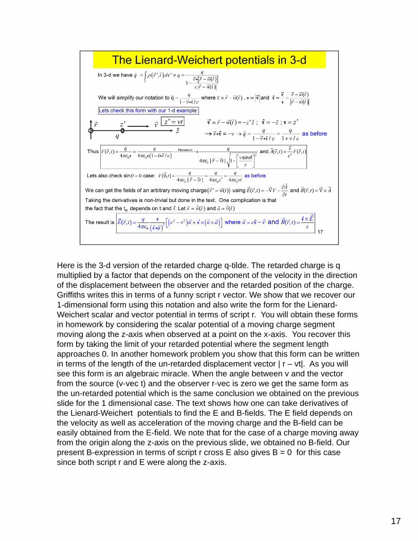
Here is the 3-d version of the retarded charge q-tilde. The retarded charge is q multiplied by a factor that depends on the component of the velocity in the direction of the displacement between the observer and the retarded position of the charge. Griffiths writes this in terms of a funny script r vector. We show that we recover our 1-dimensional form using this notation and also write the form for the Lienard-Weichert scalar and vector potential in terms of script r. You will obtain these forms in homework by considering the scalar potential of a moving charge segment moving along the z-axis when observed at a point on the x-axis. You recover this form by taking the limit of your retarded potential where the segment length approaches 0. In another homework problem you show that this form can be written in terms of the length of the un-retarded displacement vector | r – vt|. As you will see this form is an algebraic miracle. When the angle between v and the vector from the source (v-vec t) and the observer r-vec is zero we get the same form as the un-retarded potential which is the same conclusion we obtained on the previous slide for the 1 dimensional case. The text shows how one can take derivatives of the Lienard-Weichert potentials to find the E and B-fields. The E field depends on the velocity as well as acceleration of the moving charge and the B-field can be easily obtained from the E-field. We note that for the case of a charge moving away from the origin along the z-axis on the previous slide, we obtained no B-field. Our present B-expression in terms of script r cross E also gives B = 0 for this case since both script r and E were along the z-axis.

18

Lets check our form for the the Lienard-Weichert fields by recovering the Lamor power radiated by an accelerating charge for the case of zero or negligible v. We go to the far field limit to simplify our E and B expressions and find that both E and B die off as 1/r as they did in the electric dipole case. We also see that B is down by a factor of c from E, is perpendicular to E, and the Poynting vector lies along the r-hat direction. Again this is exactly the same as E and B fields generated by a dipole antenna in the far field region. In HW3 you showed that if E and B are perpendicular and B = E/c, the pointing vector is |E|^2/(mu_o c). For convenience we put the acceleration in the z-hat direction and compute |E|^2 using the bac –cab rule We find |E| is proportional to sin(theta) which means S-vec points has a factor of sin^2(theta) just like a dipole antenna. Integrating S over a sphere we get exactly the same Larmor formula for the radiated power for an accelerating charge that we did by manipulating the electric dipole antenna expression.

19

We next write down the power expression for a charge with both velocity and acceleration. The general power formula is rather difficult to obtain although it follows directly from the Lienard-Weichert potentials and involves no new physics such as relativity. The velocity appears as a pre-factor which is the same as the relativistic gamma that we will learn about shortly, and as an additional v cross a term. In the limit where v/c << 1, gamma => 1, the v cross a term is negligible and we recover the previous Lamor formula. However the gamma^6 factor greatly increases the power when the particle velocity approaches the speed of light. One interesting case is the radiation of a relativistic electron traveling in a circular orbit in an accelerator storage ring. Here the acceleration is proportional to v^2/r where r is the ring radius. We will see in our relativity chapter that gamma = energy/mc^2 which be enormous for energetic, light electrons. For example in the case we will consider (the LEP accelerator at CERN ) gamma is 100,000 and this is raised to the fourth power! By way of contrast, a proton will produce less synchrotron energy than an electron of the same energy by a factor of (1/2000)^4 which is usually pretty negligible. As we would expect from our treatment of magnetic dipole radiation, the maximum power is radiated in the orbital plane and has an electrical field, or polarization, along the direction of the current or in the orbital plane. Very little of the E-field is transverse to the plane. But interestingly enough, synchrotron radiation does not produce E&M radiation at the frequency of the circular orbit, but rather a large spectrum of energies is radiated with a critical frequency (essentially an endpoint frequency) of the circular frequency multiplied by gamma^3. Rather than producing a broad intensity pattern of the sin^2 (theta) form, the synchrotron light appears in a narrow cone like the headlight beam of a car as it travels around an arc in the road. The beam gets more tightly collimated with increasing gamma. Synchrotron radiation is both a blessing and a curse to the experimental physicist. Electrons are often the beam of choice for a high energy physicist since all of the beam energy goes into a single point-like particle (as opposed to being shared among the quark constituents of a proton). But one must pay an enormous power bill to supply the synchrotron energy radiated away by the electron or build a very large radius accelerator since to exploit the 1/r^2 factor in the power expression. On the other hand, synchrotron light provides an elegant “souped-up” x-ray source for condensed matter physicists to study and manipulate crystals. One man’s meat is another man’s poison.