In-situ observations of volcanic ash clouds from the FAAM aircraft during the

eruption of Eyjafjallajökull in 2010

Ben Johnson1, Kate Turnbull1, Phil Brown1 , Rachel Burgess2 , James Dorsey2 , Anthony J.

Baran1, Helen Webster1, Jim Haywood1,5 , Richard Cotton1, Z. Ulanowski3, Evelyn Hesse3,

Alan Woolley4, and Philip Rosenberg4

1Met Office, Fitzroy Road, Exeter, EX1 3PB, UK

2University of Manchester, School of Earth Atmospheric and Environmental

Sciences,

Oxford Road, Manchester, M13 9PL, UK

3University of Hertfordshire, Hatfield, Herts AL10 9AB, UK

4Facility for Airborne Atmospheric Measurement, Cranfield University,

MK43 0AL, UK

5University of Exeter, College of Engineering Mathematics and Physical Sciences,

North Park Road, Exeter, EX4 4QF, UK

Abstract

During April-May 2010 the UK Facility for Airborne Atmospheric Measurements (FAAM)

BAe-146 aircraft flew 12 flights targeting volcanic ash clouds around the UK. The aircraft

observed ash layers between altitudes of 2 – 8 km with peak mass concentrations typically

between 200 - 2000 µg/m3, as estimated from a Cloud and Aerosol Spectrometer (CAS). A

peak value of 2000 - 5000 µg/m3 was observed over Scotland on 14 May 2010, although with

considerable uncertainty due to the possible contamination by ice. Aerosol size distributions

within ash clouds showed a fine mode (0.1 – 0.6 µm) associated with sulphuric acid and/or

sulphate, and a coarse mode (0.6 – 35 µm) associated with ash. The ash mass was dominated

by particles in the size range 1 – 10 µm (volume-equivalent diameter), with a peak typically

around 3 – 5 µm. Electron-microscope images and scattering patterns from the SID-2H

(Small Ice Detector) probe showed the highly irregular shape of the ash particles. Ash clouds

were also accompanied by elevated levels of SO2 (10 – 100 ppbv), strong aerosol scattering

(50 - 500 x 10-6 m-1), and low Ångstrom exponents (-0.5 to 0.4) from the 3-wavelength

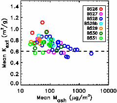
nephelometer. Coarse-mode mass specific aerosol extinction coefficients (kext), based on the

CAS size distribution varied from 0.45 – 1.06 m2/g. A representative value of 0.6 m2/g is

suggested for distal ash clouds (~1000 km downwind) from this eruption.

1. Introduction

The eruption of the Icelandic volcano Eyjafjallajökull during April – May 2010 caused major

disruption to European air travel due to prolonged emissions of volcanic ash and north-

westerly flow bringing ash clouds over the UK and much of Europe. The main period of

disruption occurred during 15 – 21 April (EUROCONTROL, http://www.eurocontrol.int) as a

cloud of volcanic ash, originating from the initial and most powerful stage of explosive

eruptions during 14 – 18 April, spread over much of Europe (Ansmann et al., 2010; Gasteiger

et al., 2011; Marenco and Hogan, 2011; Devenish et al., 2010; Dacre et al., 2011; Flentje et

al., 2010). Further episodes of volcanic ash affected the UK and western parts of Europe

from 2 – 22 May, after which explosive eruptions on Eyjafjallajökull subsided. The hazard

that volcanic ash poses to aviation is well-known (Prata and Tupper, 2009; Guffanti et al.,

2010a) and has led to major air-travel space closures in the past (e.g. Casadevall 1994;

Guffanti et al., 2010b), though none of these were on the scale experienced over Europe in

2010.

Throughout the eruption of Eyjafjallajökull the London Volcanic Ash Advisory Centre

(VAAC) provided guidance to the National Air Traffic Services (NATS) and UK Civil

Aviation Authority (CAA) based on ash forecasts produced by the Met Office Numerical

Atmospheric-dispersion Modelling Environment (NAME). NAME was configured to forecast

ash concentrations within three different flight levels; surface – FL200 (0 – 6 km), FL200 -

FL350 (6 – 10.7 km), and FL350 - FL550 (10.7 – 16.8 km), where each unit FL (flight level)

is equivalent to 100 feet assuming the International Civil Aviation Organization (ICAO)

standard atmosphere, assuming a surface pressure of 1013hPa. Initially the ash cloud was

defined as regions with significant levels of ash based on the Volcanic Ash Forecast

Transport and Dispersion (VAFTAD) table and nominal modeled release rates (Leadbetter

and Hort, 2011; Witham et al., 2007). It was later deduced that the threshold used to identify

the ash cloud extent corresponded to an estimated ash concentration of the order of 200

µg/m3. Following agreements on engine tolerance thresholds (EU 2010) three concentration

bands were established: 200 - 2000 µg/m3 (low-risk), 2000 – 4000 µg/m3 (medium risk) and >

4000 µg/m3 (high risk).

The European volcanic ash incident of April - May 2010 was also unprecedented in the

number of research-quality measurements that were made of airborne volcanic ash across

Europe and the northeast Atlantic (for an overview see Haywood et al., this issue and

references therein). Prior to the 2010 eruption of Eyjafjallajökull intensive measurements of

airborne volcanic ash have been rather limited. Previous airborne in-situ measurements of

volcanic ash include the incidental sampling from the eruption of Hekla, Iceland, during 2000

(Hunton et al., 2005; Rose et al., 2006), sampling of plumes from US volcanoes Mt. Baker

(Radke et al., 1976), Mt. St. Helens (Hobbs et al., 1982), and Mt. Redoubt (Hobbs et al.,

1991), and sampling of plumes from the Guatemalan volcanoes Pacaya, Fuego and

Santiaguito (Rose et al., 1980). Many other airborne observational studies have investigated

the emission of volcanic gases and production of secondary aerosols, generally from

quiescent or non-explosive eruptions (see Carn et al., 2011 for a recent review).

Observations of airborne ash from the eruption of Eyjafjallajökull during April – May 2010

were made from a number of atmospheric research aircraft (Schumann et al., 2011; Royer et

al., 2011; Bukowiecki et al. 2011; EUFAR 2010) including the UK’s BAe-146-301

Atmospheric Research Aircraft that is managed by the Facility for Airborne Atmospheric

Measurements (FAAM). Observations also included combinations of ground-based lidars and

sunphotometers (Marenco and Hogan 2011; Ansmann et al., 2010; Gasteiger et al., 2011;

Chazette et al., 2011), ground-based in-situ sampling (Flentje et al., 2010; Bukowiecki et al.

2011) and a balloon ascent (Harrison et al., 2010). In addition, satellite remote sensing

products were used operationally and explored in post-event analysis (Clarisse et al., 2010;

Francis et al., 2011; Newman et al., this issue; Millington et al., this issue; Baran, this issue).

The remote sensing measurements made by the FAAM aircraft are detailed in Marenco et al.,

(2011), and Newman et al., (this issue). A comparison of FAAM aircraft in-situ

measurements with those made by the Deutsches Zentrum für Luft- und Raumfahrt (DLR)

Falcon 20E atmospheric research aircraft is presented in Turnbull et al. (this issue). Whilst

many of these observations were gathered with an immediate priority of verifying the

presence, geographic extent and maximum mass concentration of ash clouds, the datasets

serve as a major opportunity for research into the properties of airborne volcanic ash, the

development of in-situ measurement and remote sensing capabilities (including satellite data

products), and the validation of ash emission and dispersion models.

A large number of ash mass concentration estimates are compared with NAME dispersion

model forecasts in Webster et al. (2011). Also, Stohl et al. (2010) use a mixture of airborne

and satellite observations to constrain and evaluate simulations of volcanic ash emission and

dispersion via the FLEXPART Lagrangian particle dispersion model. The results from each

of these studies show broad agreement in the magnitude of modeled and observed ash mass

concentrations despite large uncertainties in both the measurements and modelling of volcanic

ash. Webster et al. also highlight the large discrepancies that can arise when comparing

modeled and observed ash concentration due to even smaller errors in the timing and/or

position errors of ash clouds. Such errors are in some cases a clear reflection of errors in

numerical weather prediction model fields (Devenish et al., 2011; Stohl et al., 2011; Dacre et

al., 2011; Devenish et al., this issue). On the other hand, the specification of emission source

strength, near-source fallout, the relationship between model predicted mean concentrations

over large volumes and localised peak concentrations unresolved by the model, and the

vertical profile of ash emission also appear to be dominant sources of model uncertainty and

model-measurement discrepancy in the above studies. Devenish et al. (this issue) also show

that reducing particle sizes (bringing the prescribed size distribution closer in line with the

FAAM aircraft measurements that are reported here) improves the forecast position of ash

clouds on certain occasions, due to the reduction of sedimentation rates. Other important but

less dominant sources of model uncertainty include the treatment of vertical and horizontal

turbulent mixing (Devenish et al., this issue).

This study presents in-situ measurements recorded aboard the FAAM aircraft during a series

of flights investigating ash clouds around the UK from 20 April to 18 May 2010. The paper

provides an overview of the FAAM aircraft flights (section 2), aircraft instrumentation

(section 3), the methods used to derive ash mass concentration (section 4), and the physical

and optical properties of ash (section 5).

2. FAAM aircraft flights

2.1 Overview of the FAAM aircraft deployment

The FAAM aircraft was deployed during April - May 2010 to investigate volcanic ash clouds

in the region around the UK that were affecting domestic and international air travel. This

unplanned deployment brought the aircraft out of scheduled maintenance and into service on

20 April. A total of 12 flights were conducted on 9 separate days between 20 April – 18 May

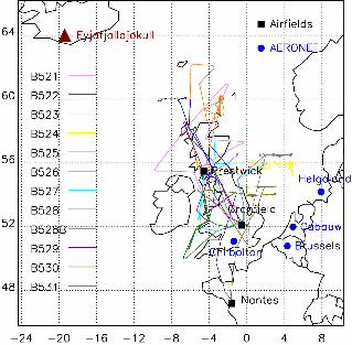
(Table 1 and Figure 1), making a total of approximately 54 flight hours. These included 9 full

length flights of 5 - 5.5 hours and three shorter flights of 1 - 2 hours. The primary objectives

of all flights were to investigate the mass concentrations of ash and the geographic and

vertical extent of those ash layers. The three shorter flights (B522, B525, B528b) were

conducted to increase time in regions of interest and / or reposition the aircraft to an alternate

airfield. The main airfields used were Cranfield (central England: 52.1°N, 0.6°W), Prestwick

(southwest Scotland: 55.5°N 4.6°W), Cambridge (central-eastern England: 52.2°N 0.2°E) and

Nantes (northern France: 47.2°N 1.6°W) (Table 1 and Figure 1).

As a four turbine-engine driven aircraft, the FAAM aircraft was subject to the same stringent

safety criteria as applied to aircraft operating under CAA regulations. On the flights during 20

– 21 April (B521 - B523) the FAAM aircraft therefore avoided penetrating ash clouds and

focussed on remote sensing of ash layers from high altitudes ( > FL200 ~ 6 km) using the

lidar. This ash avoidance policy was to satisfy CAA and internally agreed limits that were in

place at that time. From 22 April onwards volcanic ash exposure safety limits were specified,

and FAAM research flights were permitted to profile through ash layers provided NAME

forecast ash concentrations were below 2000 µg/m3. Avoidance measures were taken if real-

time in-situ monitoring showed concentrations approaching this threshold. This led to the

aircraft targeting zones where forecast volcanic ash concentrations were in the range 200 -

2000 µg/m3.

2.2 Flight objectives

The main objectives of the ash flights were:

1) To provide near real-time guidance on the spatial extent and mass concentration of

ash clouds over the UK region (for the CAA and the NATS, Met Office and London

VAAC).

2) To validate NAME simulations of ash dispersion (during and post-event analysis).

3) To investigate the physical, chemical and optical properties of transported volcanic

ash for improvements in modelling, measurement and remote sensing capabilities.

4) To explore relationships between ash mass, aerosol scattering and trace gas

concentrations including sulphur dioxide.

3. Instrumentation & modelling

The FAAM aircraft was equipped with a comprehensive range of instruments measuring

standard meteorological parameters, aerosol and cloud properties, concentrations of key

gaseous chemical species, solar and terrestrial radiation. A 355 nm lidar was also used to

remotely sense aerosol and cloud below the aircraft. A list of all scientific instruments fitted

and operated during the flights presented in this study is provided in Table 2. As this study

focuses on the in-situ characterization of the ash only the instruments relied on for this study

are described below. A general description of meteorological can be found in Renfrew et al.

(2009) and further details of FAAM aircraft instrument systems are available at

www.faam.ac.uk.

3.1 PCASP (fine-mode aerosol)

Concentrations of fine aerosols within the size range 0.1 – 3.0 µm (nominal diameter) were

measured using a wing-mounted Particle Measuring System (PMS) Passive Cavity Aerosol

Spectrometer Probe 100X (PCASP), with SPP200 electronics. The PCASP sizes particles

based on the scattering of a 632.8 nm laser beam across scattering angles of 35 – 120o, plus 60

– 145° (Garvey and Pinnick 1983; Liu et al. 1992). The PCASP instrument was calibrated

σusing laboratory generated ammonium sulphate, size-segregated by a differential mobility

analyser. The calibrated bin boundaries were corrected assuming a refractive index of 1.43 +

0i, based on the properties of sulphuric acid. We assume this to be the dominant fine-mode

aerosol species within volcanic ash clouds where, in our observations SO2 concentrations

often remained highly elevated (e.g. > 10 ppbv). Sulphate, nitrate, and other components were

also likely to have contributed to the fine mode as found by Schumann et al. (2011), in

addition to variable amounts of water. However, due to heaters within the PCASP the

measured aerosol was unlikely to have contained appreciable water (Strapp et al., 1992). The

refractive index of such a mixture is likely not far from the value we assume. The fine-mode

aerosols are assumed to be spheres enabling the use of Mie-Lorenz theory to calculate

scattering properties.

3.2 CAS (coarse-mode aerosol)

Concentrations of coarse aerosols of nominal diameters 0.6 – 50 µm were measured using the

Cloud and Aerosol Spectrometer (CAS), a component of the Droplet Measurement

Technologies (DMT) Cloud Aerosol and Precipitation Spectrometer (CAPS) probe

(Baumgardener et al., 2001). The CAS is a wing-mounted optical particle counter. The air

sample is drawn through a cylinder of 33 mm diameter and 485 mm length. The optical

sample volume of approximately 0.24 mm2 is positioned mid-way along the length of the

cylindrical path and at its radial centre. The CAS uses forward scattering (4 – 12°) of a 680

nm laser beam to size particles. The CAS was calibrated by the manufacturer using a

combination of PSL spheres (for d < 2 µm), borosilicate glass beads (2 µm < d < 20 µm) and

soda lime glass beads (20 µm < d < 50 µm). The larger size bins (d > 10 µm) were checked

pre-flight using glass beads and found to be sizing well with discrepancies no greater than the

typical diameter spacing between adjacent bins ( ~ 15%). Mie-Lorenz theory is then used to

calculate the scattering cross-section of the calibration spheres across the instrument’s 4 -12°

forward scattering angular detection range. This provides a calibration relating the amplitude

of the instrument’s response to particle scattering cross-sections. Using Mie-Lorenz theory

the nominal size bin limits can then be defined in terms of the diameter of water droplets

having the same scattering cross-section. However, in this study the bin boundaries are

defined in terms of the volume-equivalent diameter of irregularly-shape ash particles via a

more complex treatment of scattering (as outlined in section 4.2). The estimation of particle

concentration per unit volume of air depends on the air-speed through the CAS inlet.

Although the CAPS is equipped with a pitot sensor for the calculation of air-speed the results

from this instrument did not seem realistic compared to the true air-speed, indicated by the

turbulence probe on the nose. Therefore the later instrument was used to provide the estimate

of air-speed.

The CAS data were also quality checked by examining the distribution of signal amplitudes in

each gain stage from the raw particle-by-particle data, which contained the precise signal

amplitudes (digital counts) for up to 292 particles per second. The use of three gain stages is

required to span the very large range of scattering amplitudes ( ~ 4 orders of magnitude) that

arise across the CAS size range. In this way the measurement of aerosol size is partitioned

into three size ranges. The analysis revealed dips in the histogram of scattering amplitudes

corresponding to the beginning of each of the three gain stages. These corresponded to slight

dips in the derived aerosol size distribution in transitions between gain stages. This problem

was attributed to insufficient restoration of baseline voltages on each gain stage between

particle detections. A problem of this nature leads to some particles being oversized (placed in

a bin too high for their true size), but would not have led to over-counting or under-counting.

Although no formal correction for this problem has been proposed a reasonable attempt has

been made to adjust the data for this error. Within the post-flight data interpretation the signal

amplitude thresholds for each bin were adjusted by assuming a larger voltage offsets on each

gain stage than are assumed normally in the real-time data processing. The voltage offsets

were tuned to ensure a smooth and continuous distribution of signal amplitudes across the

entire range of measured signal amplitudes. This correction did not alter the total number of

particles, nor the number counted in each bin but led to changes in the lower and upper

diameters for each size bin. Corrections for particle shape and refractive index are explained

in section 4.2 and the sensitivity to those assumptions is assessed in section 5.5.1.

3.3 SID-2H (coarse-mode aerosol scattering patterns)

An improved version of the Small Ice Detector 2 (SID-2) (Hirst et al., 2001; Cotton et al.,

2009) was also fitted and used to determine the scattering patterns and asphericity of particles

of diameters > 2µm. SID-2 is an optical particle counter that measures the intensity of

forward scattered light across scattering angles of 9 – 20o and its azimuthal variation using

independently sensed detector elements. The improved version, named SID-2H, uses for this

purpose 28 elements of a multi-channel photomultiplier coupled via fiber-optics guides

(Ulanowski and Schnaiter, 2011). Whilst the data from SID-2H can be used to estimate

particle size distributions, the asphericity of the particle’s scattering also gives clues to the

particle shape and hence composition. Originally the SID instruments were developed to

allow the discrimination between super-cooled water drops and ice crystals in the diameter

range 1 – 24 µm. However, recent measurements in Saharan dust (Johnson and Osborne,

2011) have shown that SID-2H is capable of measuring the scattering from coarse mineral-

dust particles (d > 2 µm). The SID-2H instrument was calibrated using PSL (latex) spheres, as

described in Cotton et al. (2009). This calibration is given in nominal diameters relevant to

water spheres. However, due to various issues regarding signal amplification (gain), and

triggering thresholds the sizing performance of the probe in these flights was uncertain. The

SID-2H data is therefore used in this study mainly for qualitative examination of aerosol

scattering patterns.

3.4 Nephelometer (aerosol scattering coefficients)

Aerosol scattering was determined at three wavelengths (0.45, 0.55, 0.70 µm) with a TSI

3563 nephelometer. Angular truncation errors were corrected following the super-micron

relations in Anderson and Ogren (1998). The air sample is drawn from a Rosemount inlet and

transmitted through ~ 2 m pipes comprised of latex rubber infused with black-carbon. All

components of the inlet and pipe-work are electrically conductive and earthed to prevent the

build up of static charge that would lead to aerosol losses. The Rosemount inlet is not

designed for aerosol sampling and as yet its sampling efficiency is not fully understood.

When the TSI instrument was situated on the C-130 aircraft during the SHADE measurement

campaign in 2000 (Tanré et al., 2003), a significant correction had to be made to account for

the loss of super-micron aerosol particles in the inlet/pipe-work (Haywood et al., 2003).

Recent tests at FAAM (personal communication JaMie-Lorenz Trembath) suggest that the

Rosemount inlet looses some particles greater than 5 µm diameter but may oversample

particles in the diameter range 1 – 5 µm. Comparison of aerosol optical depths derived from

the nephelometer when the TSI instrument was situated on the BAe-146 aircraft against

Aerosol Robotic Network (AERONET) sun-photometers during DABEX (Osborne et al.,

2008) suggests either that the majority of super-micron dust particles are sampled or that the

under and over sampling biases across the super-micron range compensated in that set of

measurements. As correction factors for such sampling issues are not yet developed at the

time of this study, no correction for super-micron particle losses was made.

3.5 Cloud ice measurements

Bulk ice water content was measured using a Nevzorov hot-wire probe (Korolev et al.,

1998a). This has a heated conical collector facing into the airstream. Ice crystals are collected

within this cone and then melted and evaporated. The collector is maintained at a constant

temperature and the additional electrical power required for this in cloud is equated to the

latent heat of evaporation of the cloud ice. The instrument has a sensitivity of around 0.002

gm-3. The absolute accuracy is dependent on the removal of altitude and temperature

dependent baseline drifts which are of order 0.005 gm-3 km-1. Recent tests by Korolev

(personal communication) have suggested that the standard collector may underestimate the

true ice water content, especially for larger ice particles, by a factor of ~ 3. This is due to the

loss of water mass from the collector prior to its evaporation via a combination of particle

bouncing or the splashing out of meltwater by subsequent incoming particles. This is

alleviated in recent versions of the probe which use deeper collector cones but these were not

fitted at the time of the flights described here.

The Cloud Imaging Probe (CIP) is an updated version of the 2D Optical Array Probe

(Korolev et al., 1998b) manufactured by DMT. A 64-element array of photodiodes is

illuminated by a laser beam. Ice crystals passing through the beam shadow the array. By

means of sampling the array at a suitably high rate, a digitized shadow image of the particle is

recorded. In the version described here (which is another part of the DMT CAPS instrument,

see section 3.2 above), the optical magnification is such as to give a pixel resolution in the

array-parallel direction of 15 μm and the instrument is referred to as the CIP-15. Images are

processed to determine their linear dimensions and, by means of the use of suitable size-to-

mass conversion factors, their mass. In the data described here, the size-mass factors are those

given by Brown and Francis (1995) and the total ice water content is obtained by integration

over the full size spectrum.

3.6 Filter measurements

The filter sampling system on board the FAAM aircraft is described by Formenti et al (2008),

and consists of a thin-walled metallic inlet nozzle with a curved leading edge. The design was

based on criteria for aircraft engine intakes at low Mach numbers (Andreae et al., 1988). This

design reduces distortion of the pressure field at the nozzle tip and the resulting problems

associated with flow separation and turbulence. A curved metallic pipe feeds the air sample

into the cabin and directly into a short diffuser ( ~ 20 cm) ahead of teflon stacked-filter units.

Two of these inlet and filter systems are mounted in parallel. The aerosol intake system was

designed so that rain and large cloud water droplets would be removed from the sampled air

stream by inertial separation. The passing efficiency of the inlets has not been formally

quantified. However, Chou et al. [2008] have shown that the number size distributions of the

aerosols collected on the filters (counted by electron microscopy) extended up to 10 μm

diameter and were comparable to those measured by wing-mounted optical counters. Because

the sampling is sub-isokinetic, a relative enhancement of the coarse particle fraction might be

expected. Each stacked filter unit consisted of two 47 mm Nuclepore filters of 10 and 1 µm

pore diameter. Filters were exposed for extended periods (usually half or whole of a flight) to

gain sufficient mass loading but exposure was interrupted during passes through cloud or

boundary layer aerosol to avoid contamination.

Scanning Electron Microscope (SEM) imagery and elemental analysis of the aerosol collected

on the filters was carried out at the University of Manchester using a Phillips FEI XL30

Environmental Scanning Electron Microscope (ESEM) equipped with a Super Ultra-thin

Window and EDAX™ automatic particle analysis software (Hand et al, 2010). The SEM was

operated with the back-scatter detector and beam energy of 15 kV (occasionally 20 kV). After

the initial focussing the SEM was controlled using the EDAX Genesis software to

automatically image the required number of fields of view, scan and collect spectra for each

automatically identified individual particle. For each individual particle several

morphological features are recorded and also some information on the chemical composition

is achieved from the spectra yielded from the energy dispersive x-ray (EDX). The chemical

composition analysis is ongoing and will not be discussed here. However, initial results

showed the dominant elements in the majority of the particles analysed were Si, Al, and Mg,

and had signature compositions of volcanic ash. Fe was also observed in approximately half

of these Si and Al containing particles. The presence of Ti, K and Ca was also detected in

some of the particles though not necessarily simultaneously. A full description of the

chemical and morphological characteristics of the sampled particles will be given in a

separate paper (Burgess et al in prep).

3.7 Gas phase measurements

Gas phase chemistry measurements of sulphur dioxide (SO2) were made using a Thermo

Electron 43C Trace Level analyzer which relies on pulsed fluorescence (Luke, 1997). This

has a detection limit of 0.005 ppbv and a precision of 1% or 0.2 ppbv (whichever is greater).

The instrument was calibrated prior to the series of flights using a bottled gas standard. This

provides 10 second averages but the low sample flow rate (0.5 L/min) leads to a time lag of ~

25 seconds and some loss of time resolution. Data were corrected by allowing a 25 second

time lag relative to the real-time data (i.e. fast response instruments such as the wing-mounted

OPCs). The effective time resolution of the data appears to be around 20 s making the data

more suitable for identifying broad features (dz ~ 300 m, dx ~ 10 km) during profiles or runs,

or averages over ash cloud penetrations of at least 1 min.

3.8 AERONET data

AERONET data (Holben et al., 1998) were obtained from http://aeronet.gsfc.nasa.gov. The

sites of Helgoland (54.2°N, 7.9°E), Brussels (50.8°N, 4.3°E), and Cabauw (52.0oN, 4.9°E)

were selected for the period from 1500UTC on 17 May to 1800UTC on 18 May. Almucantar

scans were used in conjunction with version 2 inversion algorithms to retrieve aerosol size

distribution. The version 2 algorithm includes a representation for particle asphericity via

randomly orientated prolate and oblate spheroids (Dubovik et al., 2006).

3.9 NAME model

The Numerical Atmospheric-dispersion Modelling Environment (NAME) is a Lagrangian

particle model that was used to simulate the dispersion of ash from the 2010 eruption of

Eyjafjallajökull. It was driven by meteorological data from the global version of the Met

Office's Unified Model (MetUM) with a spatial resolution of about 25 km in mid latitudes

and a temporal resolution of 3 hours. A full description of NAME and its set-up for

simulations of ash from the 2010 Eyjafjallajökull eruption are given in Webster et al. (2011).

The dispersion simulations presented in this study are from a post-event simulation. The set-

up was identical to that used operationally towards the end of the eruption except that

analysed, as opposed to forecast, meteorological data were used. The mass emission rate was

calculated using the continuous fit to the VAFTAD thresholds (Webster et al., 2011). The

simulations are therefore an attempt to producing the best possible post-event analysis in the

absence of data assimilation or user intervention. The mass emission rate is estimated from

the observed eruption height using an empirical relationship between these two quantities.

95% of the erupted mass is assumed to fall-out near to the source (i.e. only 5% is assumed to

survive into the distal ash cloud). Loss of ash due to gravitational settling of heavy particles

and wet and dry deposition processes is represented within NAME. The particle size

distribution used for volcanic ash is based on measurements from explosive eruptions of

Mount Redoubt, St Augustine and Mount St Helens as presented by Hobbs et al. (1991).

Average concentrations are calculated over 6-hour time periods and over deep atmospheric

layers (0 – FL200 [approx 0 – 6 km], FL200 – 350 [approx 6 – 10.7 km], FL350 – 550

[approx 10.7 – 16.8 km]). The peak concentration likely to occur in these deep layers and 6-

hour time periods is assumed to be a factor of 20 higher than the large-scale modeled mean

concentration.

4. Derivation of ash particle size distribution and mass concentration from the

CAS instrument

4.1 Method of deriving ash mass concentration

The aerosol size distribution was segregated into a fine mode (0.1 – 0.6 µm), measured by the

PCASP and assumed to be sulphuric acid aerosol, and a coarse mode (0.6 – 35 µm), measured

by the CAS and assumed to ash. The cut-off at 0.6µm was based on size-resolved chemical

composition results from Figure 6 of Schumann et al. (2011) and the observed minima in the

PCASP and CAS mass distributions (see section 5.3.1). In this study, only bins 2 – 26 of the

CAS are used, covering volume-equivalent diameters of 0.6 – 35 µm (see Table 3). The first

bin was rejected as the lower limit of its diameter range was poorly defined. The largest four

bins of the CAS (bins 27 – 30) were rejected from the analysis as these returned zero or

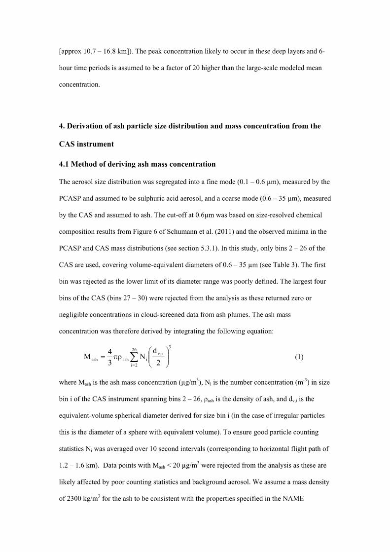
negligible concentrations in cloud-screened data from ash plumes. The ash mass

concentration was therefore derived by integrating the following equation:

26

2i

3

i,viashash 2

dN

3

4M (1)

where Mash is the ash mass concentration (µg/m3), Ni is the number concentration (m-3) in size

bin i of the CAS instrument spanning bins 2 – 26, ρash is the density of ash, and dv,i is the

equivalent-volume spherical diameter derived for size bin i (in the case of irregular particles

this is the diameter of a sphere with equivalent volume). To ensure good particle counting

statistics Ni was averaged over 10 second intervals (corresponding to horizontal flight path of

1.2 – 1.6 km). Data points with Mash < 20 µg/m3 were rejected from the analysis as these are

likely affected by poor counting statistics and background aerosol. We assume a mass density

of 2300 kg/m3 for the ash to be consistent with the properties specified in the NAME

dispersion model (Webster et al., 2011). This may be regarded as a low estimate compared to

published values for solid volcanic glasses and minerals (typically 2350 – 3000 kg/m3, e.g.

Shipley and Wojcicki 1982; Sparks et al., 1997; Mastin et al., 2009; Gudmundsson et al.,

2010; Schumann et al., 2011) but accommodates the possibility of air pockets within

aggregates and larger particles (e.g. James et al., 2002, 2003). Volume-equivalent diameters

were derived by modelling the optical properties of ash and the scattering response of the

CAS instrument. As this requires assumptions on particle shape and refractive index three

cases have been considered (Table 3).

4.2 Refractive index and particle shape assumptions

The assumptions used to process the CAS and PCASP data are detailed in Table 3. In the

default case “ash irregular” the ash (i.e. the coarse-mode measured by CAS) is represented by

irregular-shaped particles and a refractive index of 1.52 + 0.0015i, based on the mineral dust

dataset of Balkanski et al. (2007) with the medium level of hematite (1.5%). Although the

mineralogy of volcanic ash differs from that of desert dust estimates for the refractive index

are similar. Current estimates for volcanic glasses and minerals suggest real parts between

1.50 – 1.60 and imaginary parts generally between 0.001 – 0.004i for the wavelengths around

600 – 700 nm (Patterson 1981; Patterson et al., 1983; Pollack et al. 1973; Horwell 2007;

Schumann et al., 2011; Oskarsson 2010). The Balkanski et al. (2007) refractive index dataset

has also proved successful in modelling upwelling solar and spectrally resolved longwave

radiation when compared with observations taken above ash layers from both the FAAM

aircraft Airborne Infra-Red Interferometer Evaluation System (ARIES), and the Infra-red

Atmospheric Sounding Interferometer (IASI) satellite instrument (Newman et al., this issue).

The irregularity of ash particle shapes have been represented using a method previously

applied to mineral dust, as described by Osborne et al. (2011). This treated the particles as a

mixture of hexagonal prisms of aspect ratio unity (for 0.6 < dv < 1.5 µm), and polyhedral

crystals (for 1.5 < dv < 35 µm). The polyhedral model is based on work by Macke et al.

(1996) which was originally applied to study the scattering properties of cirrus but has

successfully been applied to large mineral dust aerosols by Kokhanovsky (2003) and Osborne

et al. (2011). The scattering properties in this study were calculated from the Ray Tracing

with Diffraction on Facets (RTDF) method (Hesse, 2008). This differs from classical

geometric optics by considering diffraction at facets in addition to diffraction at the projected

cross-section and therefore describes the size-dependence better, especially for the size range

included in this study (1.5 – 35 µm), which are small compared to those of ice crystal. Due to

this, the calculations are different from those of Kokhanovsky (2003) even for the same

crystal geometry. Although detailed analysis has not yet been performed to assess the

applicability of this model to the volcanic ash, the fractal-like irregular shapes it uses are

arguably a more realistic representation of ash than the smooth, compact and symmetrical

geometry of spheres or spheroids (Osborne et al., 2011). Irregular shapes are evident in

electron microscope images of volcanic ash for Eyjafjallajökull (see section 5.4.1 and

Navratil et al., this issue). Further research would be required to refine the assumptions used

in the polyhedral model based on statistical analysis of SEM images and/or SID-2H data.

Two spherical ash treatments are also used (Table 3) as sensitivity tests. The “ash sphere” has

the same refractive index as the default “irregular ash” case (1.52 + 0.0015i), and the “more

absorbing ash sphere ” is a case with refractive index raised to 1.59 + 0.004i, following

Schumann et al. (2011). The optical properties for the spherical ash cases were derived from

Mie-Lorenz theory.

4.3 Cloud screening of ash data

All flight data were manually screened for cloud using a combination of evidence from: (1)

visual observations reported from the flight deck, (2) hygrometers indicating saturation with

respect to liquid water or ice, (3) significant returns ( > 10-3 g /m3) from the Nevzorov total

water content probe, (4) sudden orders of magnitude increases in CAS particle volume

dominated by particles of nominal diameters 10 – 50 µm, (5) an extension of the particle size

distribution into diameters > 50 µm on the SID-2H and CAPS Cloud Imaging Probe (CIP-15),

indicative of ice aggregates and/or precipitation, (6) dramatic increases in CAS particle

volume that were not correlated with, or highly disproportionate to the nephelometer aerosol

scattering or SO2 concentration. In water cloud and thick patches of cirrus, cloud was easily

identifiable from the above indicators.

5. Results

5.1 Spatial distribution of ash and comparison with NAME forecasts

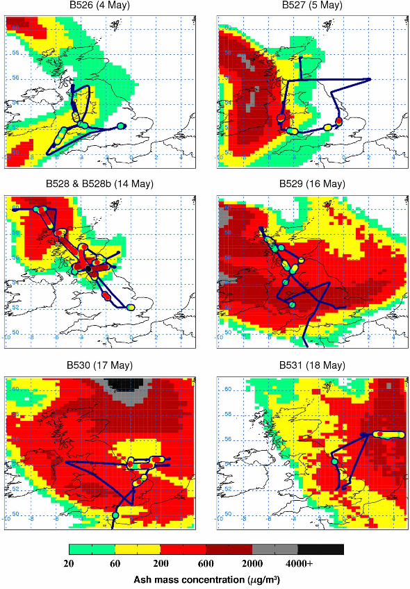
Figure 2 shows the flight tracks of the FAAM aircraft for flights B526 - B531 (4 – 18 May)

with Mash (the CAS estimate of ash mass concentration from equation 1) shown along each

flight track. The earlier flights of B521 - B525 (20 - 22 April) are not shown as very limited

in-situ sampling was coducted on those flight and observed ash concentrations did not exceed

30 µg/m3. The majority of substantial ash concentrations (> 200 µg/m3) were observed during

the flights of 4 – 18 May (B526 - B531) and for this reason the results below focus mainly on

these flights. The spatial distribution of the data in Figure 2 is shown in relation to ash

concentrations predicted by the NAME dispersion model. Flight plans tended to be spatial

extensive to survey regions where ash had been forecast at concentrations > 200 µg/m3,

and/or SEVIRI imagery had suggested ash clouds. As significant portions of many of the

flights were conducted at high altitudes, typically FL250 – 300 (7.5 – 9 km, see Figure 3), to

enable remote sensing by nadir pointing instruments, fair comparisons between Mash and the

model can only be made in those regions where a full vertical profile spanning the ash

layer(s) was made (see Figure 3). Therefore the comparison in Figure 2 must not be taken at

face value but must be interpreted carefully following the detailed flight-by-flight comments

below. These NAME dispersion simulations indicate the maximum concentration likely in

any particular region over a 6 hour time window and in a given altitude range, in this case

from the surface to FL200 ( ~ 6 km). Due to the chaotic and turbulent nature of the

atmospheric flow at the volcanic source and during subsequent advection, NAME does not

attempt to make a deterministic prediction of ash concentration fields downwind. Rather the

simulated fields indicate the possibility (or risk) of encountering ash concentrations between

certain limits in a broad time window and altitude band. The goal of this section is therefore

to see if the maximum observed ash concentrations would have been anticipated given the

best possible simulation from NAME. The FAAM in-situ ash concentration estimates are

compared to NAME simulations in a more statistical manner by Webster et al. (2011). Further

comparisons between NAME and the aircraft in-situ and remote sensing data are given by

Devenish et al. (this issue) for the 14 May case. Comparisons of the NAME simulations with

FAAM lidar retrievals of ash mass are also shown by Marenco et al. (2011).

B526 (4 May): Flight B526 surveyed an ash cloud over Wales, the Irish Sea and the Bristol

Channel. The flight plan included three overpasses of a ground-based observing site at

Aberystwyth (52.5°N, 4.1°W) to enable comparison of aircraft with ground-based lidar

measurements (Marenco et al., 2011). The bulk of the in-situ measurements gathered during

this flight are from a pair of profiles over the Irish Sea and a brief descent into an ash layer at

5km over the northwest tip of Wales (see Figures 2 and 3). These show the dispersion

simulation to have correctly predicted an ash layer in those regions with an appropriate range

of mass concentrations (60 – 200 µg/m3).

B527 (5 May): Flight B527 investigated an ash cloud encroaching from the northwest. The

lidar and in-situ sampling during profiles reveal that some of the ash cloud extended further

east over the UK than predicted in the NAME simulation (Figure 2). The excursion over the

North Sea found the edge of the ash cloud (perceptible by lidar) at ~ 0o longitude. On this day

most of the ash was found in a thin layer between 3 and 4 km with peak concentrations of 200

– 600 µg/m3. Tenuous layers with concentrations 20 – 200 µg/m3 were also encountered in a

few locations at 7 – 8 km (see Figure 2 & 3). The peak concentrations obtained during the

profiles over the Irish Sea show good agreement with the NAME simulation but the final

profile into Cranfield exceeds the simulated peak. This discrepancy was associated with a

more limited eastwards progression of the modeled ash cloud than observed (see Marenco et

al., 2011).

B528 (14 May): Flight B528 took the aircraft to the far northwest approaches of Scotland to

investigate an ash cloud encroaching over Scotland. This flight provided the most substantial

quantity of in-situ sampling data and the highest ash concentrations of the series of flights

presented here. The CAS observed higher ash concentrations than NAME simulated,

particularly over central and southern Scotland. Peak estimates of ash concentration were

difficult to disentangle from the influence of ice (appendix B) but are estimated to have

reached 2000 - 5000 µg/m3. Devenish et al. (2011) provides a full investigation of the ash

dispersion simulations for this case study and their sensitivity to various modelling

assumptions. The ash observations made over Central England 52 – 53°N were obtained

around 1900 UTC and fall outside the validity time of the NAME simulation in Figure 2

(1200 - 1800 UTC). This is a source of discrepancy between those observations and the

NAME field shown.

B529 (16 May): On 16 May a large swathe of ash was forecast to cover the UK. Peak

concentrations of 200 - 2000 µg/m3 below altitudes of 6 km ( < FL200) are shown in the

NAME simulation (Figure 2). The aircraft flew over central and northern England, Wales and

Scotland and observed ash layers with the lidar between 3 and 6 km. Lidar-derived ash mass

concentrations of up to 1000 µg/m3 (Marenco et al., 2011) were in good agreement with

NAME. Due to the high concentrations ( > 2000 µg/m3) in the forecast that was available at

the time of the flight, the aircraft was not permitted to descend below 6km (FL200). The low

concentrations of 20 - 200 µg/m3 shown in Figure 2 over those regions are therefore not

representative of peak concentrations; they are merely evidence of “skimming” the tops of

those layers (Figure 3). The profile at 1600 – 1630 UTC (Figure 3) over Wales was in largely

ash free air just beyond the southern boundary of a large band of high ash concentrations that

were observed by the FAAM aircraft lidar (Marenco et al., 2011). In the NAME simulation

ash had progressed further south over Wales and central England (Figure 2) than was

observed, either by the FAAM aircraft lidar or satellite imagery.

B530 (17 May): On 17 May the aircraft began from Nantes as it had been re-located at the

end of the previous day’s flight in anticipation of airspace closures over the UK. The NAME

simulation shows a large ash cloud with peak concentrations of 200 - 2000 µg/m3 between 0 –

6 km (0 – FL200) over most of the UK. The early part of flight B530 was conducted at high

altitudes ( > FL200 ~ 6 km) over SE England and central parts of the UK. The lidar showed

very limited evidence of ash over SE and central England and only tenuous layers over Wales

and northern England with ash concentrations mostly below 200 µg/m3 (Marenco et al., this

issue). This confirms a decision that was made to re-open low-level airspace (< FL200 ~ 6

km) on that day. The model error in this case stems from a positional error in a cloud of ash

that approached the UK from the North Atlantic on 15 May, as revealed by SEVIRI satellite

images (not shown). Directed by satellite imagery approximately 2 hours of intensive

measurements of ash were made over the North Sea during the later part of B530. As shown

in Figures 2 & 3 CAS observations of Mash of up to ~ 500 µg/m3 were encountered during a

series of profiles around 54°N, 0 - 2°E. A full exploration of those in-situ measurements and

the accompanying remote sensing measurements are provided by Turnbull et al. (this issue)

and Newman et al. (this issue), respectively.

B531 (18 May): On May 18 the aircraft investigated the edge of an ash cloud travelling down

northeastern parts of the North Sea. No significant ash was observed over eastern England but

ash layers were observed over the North Sea by the lidar (see Marenco et al. 2011). In the

NAME model some ash was still present over central and eastern parts of England and

Scotland due to the earlier positional error that was noted on 16 and 17 May. An intensive

pattern of profiles and runs for in-situ and co-located remote sensing was conducted over the

North Sea. Lower concentrations of ash (maximum ~ 200 µg/m3) were observed, compared to

the previous day’s flight.

5.2 Peak concentrations and column loadings

Ash cloud penetrations have been defined in this study as sections of data where Mash

(equation 1) exceeded 20 µg/m3 for more than 30 seconds (equivalent to a flight path of ~ 5

km). Ash cloud penetrations longer than 10 mins were broken into smaller sections based on

indentifying separate layers of ash within the time series. By this definition there were 61 ash

plume penetrations from the flights presented in this study (Table 4) but with the bulk of the

data from the later flights of B528 – B531 made during 14 – 18 May. Peak concentrations are

defined here as the maximum value observed (after 10 second averaging) during an ash plume

penetration. Where the ash plume maxima observations were located less than 50 km apart

only the higher peak value was retained. The range of peak concentrations given in Table 4 is

the range of values given by the largest three peaks per flight. The highest peak values per

flight vary from (30 – 4670 µg/m3) showing the observed variability across this dataset. The

ash column loadings have been derived by integrating Mash over the altitude for those profiles

that extend through the depth of all ash layers, as can be seen by comparing Figure 3 with

Figure 3 of Marenco et al., (2011). Some flights show very low column loadings < 0.1 g/m2 ,

either where the dominant ash layers were very thin (e.g. B527 on 5 May), where mean

concentrations were quite low (B526 on 4 May), or where flight plans led to the avoidance of

profiling through any of the thick ash layers (B529 on 16 May). In the case of B521 – B525

(20 – 22 April) all of the above were true.

5.3 Aerosol size distributions

5.3.1 CAS & PCASP

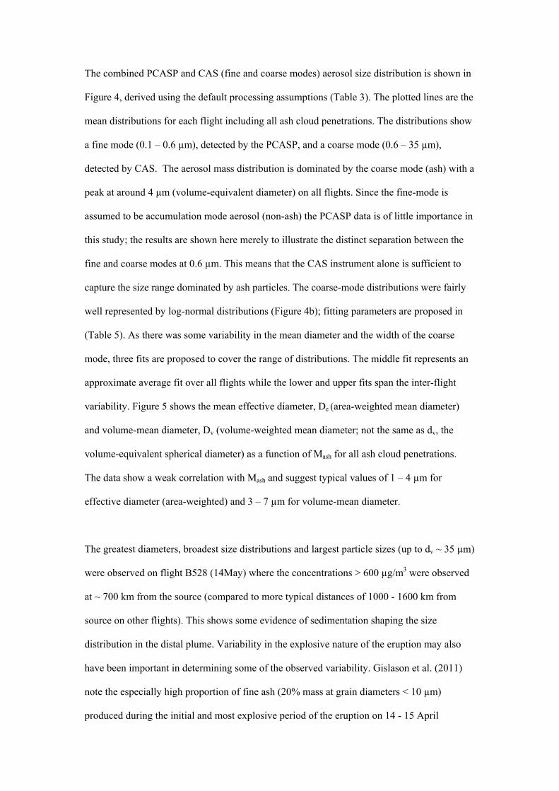
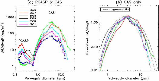
The combined PCASP and CAS (fine and coarse modes) aerosol size distribution is shown in

Figure 4, derived using the default processing assumptions (Table 3). The plotted lines are the

mean distributions for each flight including all ash cloud penetrations. The distributions show

a fine mode (0.1 – 0.6 µm), detected by the PCASP, and a coarse mode (0.6 – 35 µm),

detected by CAS. The aerosol mass distribution is dominated by the coarse mode (ash) with a

peak at around 4 µm (volume-equivalent diameter) on all flights. Since the fine-mode is

assumed to be accumulation mode aerosol (non-ash) the PCASP data is of little importance in

this study; the results are shown here merely to illustrate the distinct separation between the

fine and coarse modes at 0.6 µm. This means that the CAS instrument alone is sufficient to

capture the size range dominated by ash particles. The coarse-mode distributions were fairly

well represented by log-normal distributions (Figure 4b); fitting parameters are proposed in

(Table 5). As there was some variability in the mean diameter and the width of the coarse

mode, three fits are proposed to cover the range of distributions. The middle fit represents an

approximate average fit over all flights while the lower and upper fits span the inter-flight

variability. Figure 5 shows the mean effective diameter, De (area-weighted mean diameter)

and volume-mean diameter, Dv (volume-weighted mean diameter; not the same as dv, the

volume-equivalent spherical diameter) as a function of Mash for all ash cloud penetrations.

The data show a weak correlation with Mash and suggest typical values of 1 – 4 µm for

effective diameter (area-weighted) and 3 – 7 µm for volume-mean diameter.

The greatest diameters, broadest size distributions and largest particle sizes (up to dv ~ 35 µm)

were observed on flight B528 (14May) where the concentrations > 600 µg/m3 were observed

at ~ 700 km from the source (compared to more typical distances of 1000 - 1600 km from

source on other flights). This shows some evidence of sedimentation shaping the size

distribution in the distal plume. Variability in the explosive nature of the eruption may also

have been important in determining some of the observed variability. Gislason et al. (2011)

note the especially high proportion of fine ash (20% mass at grain diameters < 10 µm)

produced during the initial and most explosive period of the eruption on 14 - 15 April

followed by a change to a coarser (and historically more typical) ash size distribution ( < 2%

mass at grain diameters < 10 µm) during a less intensive phase of the eruption on 27 April.

The explosive nature of the Eyjafjallajökull eruption re-intensified during May and variability

in the eruption intensity, along with the rate of glacial ice falling into the eruption crater are

likely to have influenced the ash size distribution. These links have not yet been explored and

would need a more comprehensive measurement suite than those available on the FAAM

aircraft platform.

The CAS size distributions differ significantly from the measurements of Schumann et al.

(2011) where the volume peak is shown at 8 – 10 µm. Turnbull et al. (this issue) show that

this discrepancy is not entirely related to differences in assumed refractive index or particle

shape but uncertainties in instrument performance are a significant contributor. The in-situ

measurements made at the Jungfraujoch high-altitude research station (3580 m a. s. l.) gave

volume peaks at diameters of around 3 µm (Bukowiecki et al., 2011); slightly smaller than in

our results where CAS mass peaked at diameters of around 4 µm (Figure 4). This is not

surprising, given that their observations were made further downwind than ours and therefore

affected by further size-selective sedimentation. Some support for the CAS size distribution is

also provided by the successful longwave and shortwave radiative closure demonstrated by

Newman et al. (this issue). In-situ observations of airborne ash from past eruptions are

limited. Aircraft observations following the eruptions of Mt. St. Helens and Mt. Redoubt

(Hobbs et al., 1982; Hobbs et al., 1991) showed ash volume modes peaks between 10 – 30µm

but at close distances to source (10 – 170 km). Analysis of surface deposits from the Shetland

Isles (60oN, 1°W) (SEPA 2010) showed evidence of some glassy shards with dimensions of

15 – 45 µm following the mid-April phase of the eruption. An exceptional shard of 30 µm

width and 188 µm length was also found within the sample; these shards would likely shatter

to form fragments if sampled by the aircraft instrumentation.

These results can be used to refine the distribution of ash particle sizes released in dispersion

models. For example, the size distribution assumed in NAME is from Mount Redoubt, St

Augustine and Mount St Helens as presented by Hobbs et al. (1991), and has a peak for

diameters between 10 – 30 µm, with 75% of the mass at diameters > 10 µm. This contrasts

against the CAS results where typically less than 10% of the mass was in the size range dv >

10 µm. However, one can not make a direct comparison of emitted size distributions with

those observations downwind owing to size-selective processes such as gravitational settling

and deposition that shape the size distribution over time. NAME simulations in Devenish et

al. (this issue) indicate that fall out begins to have a strong effect on modeled mass

concentrations in downwind regions when a large portion of the modeled ash is associated

with particle diameters > 15 – 20 µm. The CAS observations in Figure 4 suggest that this

drop-out may dominate for dv > 10 µm. Millington et al. [2011] also provide some indication

that the NAME emitted size distribution is not in line with observations downwind from the

volcano. In their work simulated SEVIRI BT10.8 - BT12.0 and dust RGB satellite images

better matched the real satellite images when the simulated size distribution for the ash had

reduced particle sizes (peak at 5 µm), compared to emitted size distribution assumed in

NAME (peak between 10 - 30 µm). In further work, it would be interesting to compare the

NAME downwind size distribution with that observed and used to provide the best simulated

satellite imagery. Some work has already been carried out comparing NAME particle size

distributions co-located with the FAAM observations (Helen Dacre, personal

communication). Results show that NAME requires a modified effective source particle size

distribution, containing a larger fraction of sub 10um diameter particles than described above,

to capture the particle size distribution derived from the CAS measurements presented here.

This is consistent with the idea that Eyjafjallajökull emitted very fine particles due to the

interaction of volcanic ash with the ice cap (Gislasona et al. 2011). However, one can not

generalise this conclusion to all eruptions as effective source particle size distributions vary.

5.3.2 SEM analysis

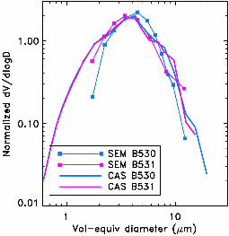
The CAS size distribution has also been compared to sizing results from SEM analysis of ash

samples collected on filters during flight. Figure 6 compare flight averaged size distributions

for flights B530 and B531 (17 & 18 May) on which the duration of in-situ sampling and filter

exposure led to both favourable filter loadings and good particle counting statistics. For flight

B530 (17 May), 4585 particles were individually analysed from the 1µm filter and 6707

particles on the 10 µm filter (310 fields of view) compared to 8273 particles from 100 fields

of view from the 10 µm filter collected on flight B531 (18 May). These filters had been

exposed continuously during all parts of the flights when ash in-situ sampling occurred and

therefore represent a flight mean. Both CAS and SEM size distributions have been

normalized to give a volume of unity when integrating dV/dlogD over the 1 – 15 µm diameter

range to allow a comparison of size distribution shape rather than absolute concentrations.

The agreement is remarkably good despite fundamental differences in the ways that dv are

derived. In the SEM analysis dv is assumed to be equal to da, the diameter of a sphere of

equivalent cross-sectional area. This may greatly overestimate the volume of particles with

large aspect ratio, especially if those particles preferentially lie flat on the filter exposing their

maximum cross-sectional area. The size range provided by the SEM analysis is more limited

than that of CAS. Particles smaller than 1µm are not all retained due to the 1 µm pore size

whereas particles larger than 10 µm may be under-sampled due to impaction within the inlet

and sample pipes. This may explain the tail off in the SEM size distribution for dv > 10 µm,

and the lack of particles for dv > 15 µm. Thus the observed SEM size distribution is to some

extent a reflection of the collection efficiency of the filter system and the apparent agreement

with CAS may be somewhat fortuitous.

5.3.3 AERONET

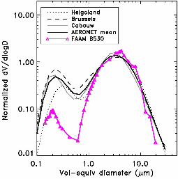
The flight mean PCASP and CAS size distribution from flight B530 (17 May) has also been

compared to size distribution retrievals from AERONET sunphotometers (Figure 7). The sites

of Helgoland (54.2°N, 7.9°E), Brussels (50.8°N, 4.3°E), and Cabauw (52.0oN, 4.9°E) were

selected for the period from 1500 UTC on 17 May to 1800UTC on 18 May as NAME back

trajectories (not shown) and satellite imagery (Newman et al., this issue) showed that, during

this period, these sites were affected by the same ash cloud that the FAAM aircraft observed

in the southern North Sea on 17 May (Figure 2). These retrievals showed strong indicators of

ash including increases in coarse-mode AOD from values of ~ 0.05 to values of ~ 0.2, and the

increased dominance of the coarse-mode (typically diameters of 0.6 – 30 µm) in the volume

size distributions (Figure 7), compared to retrievals from previous or later days in May 2010.

The plotted lines in Figure 7 are normalized by coarse-mode volume (d > 0.6 µm) to focus the

comparison on this part of the size range where ash is assumed to dominate. The site mean

AERONET retrievals are similar across the three sites peaking at 3 – 4 µm. These show

remarkably good agreement with the FAAM aircraft measurements in both the peak ( ~ 4 µm)

and width or the coarse-mode. This shows an encouraging level of consistency between the

CAS in-situ measurements and the retrievals based on observed sky radiances. As the

AERONET retrievals are sensitive to the whole aerosol column the proportion of aerosol

volume associated with the fine mode (0.2 – 0.3 µm) may be dominated by boundary layer

aerosol, which is probably of non-volcanic origin (see Turnbull et al., this issue). This may

explain why the amplitude of the fine mode is much larger in the AERONET data than in the

FAAM data, as the later did not include sampling in the boundary layer.

5.4 Ash particle shape

The shape of aerosol particles strongly influences the scattering response of optical particle

counters and therefore the derived particle size and mass. Therefore, the study of ash particle

shape is an important area of research and is examined using both SEM images and scattering

patterns detected by the SID-2H instrument.

5.4.1 SEM images

Due to the explosive nature of the eruption the ash from Eyjafjallajökull had highly irregular

non-spherical shapes including angular crystalline structures, aggregates and sharp glassy

shards (Schumann et al., 2011; Bukowiecki et al., 2011; Pyle et al., this issue; Gislason et al.,

2011). Figure 8 shows example Scanning Electron Microscope (SEM) images, taken from ash

collected on the FAAM aircraft filter system during flights B530 and B531 (17 & 18 May).

These images demonstrate the non-spherical nature of the ash and the need for more complex

treatments of irregularly-shaped particles within optical scattering models (section 4.2).

Gislason et al. (2011) show that the ash produced during the initial explosive phase on 14 -15

April and deposited ~ 55 km from the crater was especially fine-grained with sharp edges and

rough surfaces, even at sub-micron scales. Another near-source deposit collected on 27 April

when the eruption was less explosive contained larger ash particles that were considered more

typical based on previous studies from other volcanoes (Gislason et al., 2011).

5.4.2 SID-2H scattering patterns

The highly irregular shapes of ash were also evident on examining forward scattering patterns

on the SID-2H instrument. A selection of SID-2H scattering patterns is shown in Figure 9

taken from the marine boundary layer (Figure 9a) and an ash layer (Figure 9b) observed

during flight B526 (4 May). Each image is a polar plot related to the azimuthal variation of

scattered light intensity; the plot radius for each photodetector element is approximately

proportional to the square root of detector response (and therefore scattered light amplitude).

Hence plot area is proportional to particle cross sectional area and for spherical particles (with

uniform azimuthal response) plot radius is proportional to particle radius. The asphericity

factor (Af), as original devised by Hirst et al. (2001) is a dimensionless quantity varying from

0 – 100 that is proportional to the standard deviation in scattered intensity amongst the

azimuthally arranged detectors. The asphericity factor gives an indication of how far the

particle’s shape departs from spherical; it is defined as:

S

SSkA

n

i i

f

2)( (2)

Where Si is the ith detector element response out of n = 28 azimuthally arranged detectors and

k = 3.64 is a constant so that 0 < Af < 100.

The scattering patterns from the ash layer (Figure 9b) exhibit high variability in the scattering

amplitude with azimuthal angle, evidence of non-spherical shapes with high aspect ratios and

smooth facet-like surfaces (Ulanowski and Schnaiter 2011). These highly non-spherical

particles are detected for nominal diameters of ~0.5 – 6 µm. These contrast against the almost

uniform scattering patterns (Figure 9a) from aerosol sampled during a 30m run over the Irish

Sea earlier in the flight. The spherical aerosol in Figure 9a is in general larger than the non-

spherical ash of Figure 9b with nominal diameters of 3 – 12 µm. The spherical nature of the

low-level aerosol may be taken as evidence of liquid and due to the location of these

measurements we assume the aerosol to be hydrated sea-salt. As illustrated the SID-2H is

therefore a useful tool in discriminating between particle types and was used to reject CAS

data suspected to be hydrated sea-salt during low-altitude (< 300 m) sections of flight over the

sea on flights B526 (4 May) and B531 (18 May). In the absence of such information hydrated

sea-salt that had mass concentrations of ~ 200 µg/m3, as detected by CAS, may have been

misdiagnosed as being predominantly ash.

Laboratory investigations (results not shown) indicate that the ratios between forward and

back scattering, and depolarized back scattering signal provided by the CAS could be used to

discriminate between spherical and non-spherical particles, and possibly even distinguish

between ice and ash particles. The discrimination between ash and ice with SID-2H light

scattering patterns may also be possible though difficult as the light scattering patterns from

ash appear similar to some obtained from small ice particles (Cotton et al. 2010), even though

the asphericity factor appears to be somewhat higher for ash than for ice. This surprising

finding could be a consequence of the angular but smooth shape of the ash particles, as

evidenced by the SEM images. The high-resolution SID3 probe, which records images of the

forward-scatterd light was not fitted for the ash flights. However, previous flight data

obtained in a variety of ice containing clouds shows predominantly scattering patterns with

very fine, speckly structure, interpreted as being due to the dominance of particles with

irregular and/or rough surfaces (Ulanowski et al., 2010). Such patterns obtained previously in

ice clouds lead to relatively high azimuthal uniformity, when seen by the SID-2H probe.

More pristine, smooth ice crystals on the other hand produce highly non-uniform patterns

(Ulanowski et al. 2006) and such crystals could be confused with the type of ash particle seen

in this study, making it difficult to discriminate solely on the basis of low-resolution

azimuthal scattering patterns.

5.5 Uncertainties in CAS derived size distribution and mass concentration

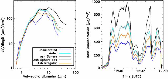
5.5.1 Sensitivity to refractive index and particle shape assumptions

Figure 10 shows the scattering cross-section of ash particles, integrated across the angular

range detected by CAS (4 – 12°), for the three cases presented in section 4.2 and Table 3, as a

function of dv. The instrument response for water spheres was also calculated (Figure 10) for

reference, as this corresponds to the nominal (uncorrected) bin diameters. These curves are

used to estimate the minimum and maximum dv for each of the 30 size bins, according to the

range of scattering amplitudes associated with each bin. On average the scattering amplitude

from the irregular ash treatment is not far from the scattering amplitude predicted for water

spheres. This occurs due to the cancellation between opposing effects of increased particle

cross-sectional area per unit volume (resulting in higher specific extinction, kext), versus

increased absorption, and a decreased preference for forward scattering. This approximate

cancellation means that the derived bin diameters (dv) for the default case (labelled as “ash

irregular” in Figure 11) are not far from the bin diameters that would be given for water,

producing similar size distributions and mass concentrations. However, the spherical ash

treatments lead to significantly lower scattering amplitudes as a function of dv, mainly due to

decreased extinction cross-section of spheres compared to irregular shapes. The increase in

the imaginary part of refractive index in the more absorbing ash sphere case leads to the

largest decreases in the scattering cross-section for dv > ~10 µm. The spherical ash treatments

lead to higher derived values of dv for the CAS bins particularly in the upper part of the size

range (dv > 10 µm), a much broader coarse mode and greatly increased Mash (Figure 11).

The example shown in Figure 11 (ash plume encountered at 60oN, 7°W on flight B528, 14

May) demonstrates the sensitivity of Mash to these assumptions. The assumption of spheres

increases the mean Mash by 24% and increases the maximum Mash by 32%, compared to the

default (irregulars) case. The assumption of more absorbing spheres increases the mean Mash

by 65% and increases the maximum Mash by 83%, compared to the irregular case. This means

the increase of refractive index alone increases mean and maximum Mash by 33% and 39% in

the spherical case. In other sections of data, particularly data samples with fewer large

particles (e.g. B526 on 4 May), the sensitivity to these assumptions was lower; the example

shown in Figure 11 demonstrates the highest sensitivity that was found from all ash flights

due to it having the highest proportion of particles above 5 µm. However, as a demonstration

of the maximum sensitivity, the results above suggests an uncertainty of ~ 50% (or a factor of

1.5) in peak values of Mash, treating the assumptions of refractive index and shape

independently. The impact of the correction for baseline offsets and consequent gain stage

overlap (section 3.2) can be seen by contrasting the “uncalibrated” and “water” results in

Figure 11. The correction delivers a smoother and more monotonic size distribution and

increases Mash by ~ 60%.

5.5.2 Uncertainty introduced by ice clouds

The uncertainty introduced by ice cloud is illustrated in Figure 12. In this profile on 14 May,

the aircraft descends through a layer in which the relative humidity is close to or just above

saturation with respect to ice. The extreme mass concentrations indicated in the unscreened

CAS data are well correlated with peaks in ice water content (IWC) derived from the CIP-15.

It is reasonable to assume that these extreme values result from the detection of cloud ice

particles by the CAS, possibly enhanced by shattering of the ice on the CAS intake tube. The

discrepancy in IWC measured by the CIP-15 and Nevzorov probe results from two issues.

Firstly a tendency for ice particles to rebound from the Nevzorov collector reduces the

measured IWC below the true value (A.Korolev, personal communication). Secondly the

baseline voltage can drift to negative values leading to an underestimation of IWC. Since

negative values could not be recorded using the data acquisition system on board at the time

of these flights, the later source of error is not correctable. Therefore the Nevzerov data from

these flights can only be used to confirm the presence of cloud and can not be used to assure

the absence of cloud. In this profile descent, the highest screened value of Mash of 4670 µg/m3

occurs at 6800m altitude, below the lowest altitude at which the CIP-15 detects ice particles

and where the relative humidity with respect to ice has fallen to around 80%. It is reasonable

to assume that these values are not directly influenced by the presence of ice particles.

Nevertheless, this region had an anomalously high ratio of Mash (4670 µg/m3) to

nephelometer-derived aerosol scattering at 550 nm ( ~ 520 Mm-1); a ratio of ~9 g/m2

compared with more typical ratio of 3 g/m2 on other parts of the flight. Also, lidar estimates

of the peak ash mass (based on aerosol extinction) reach only 1900 µg/m3 (Marenco et al.,

2011). This inferred increase in the ratio of mass to scattering or extinction is not supported

by the CAS size distribution that differs only marginally between this section of data and data

from other flights (Figure 4b). With the presently available data, it is not possible to explain

this apparent discrepancy. It may, however, be related to characteristics of the ash particles

generated by previous physical processing within cloud. For example, they may retain partial

ice coatings or their aggregation state may have been modified, generating changes in their

physical and optical properties. We suspect the screened CAS peak value in this profile to be

an overestimate but further research is necessary to explore methods of distinguishing these

kinds of problems.

5.5.3 Overall uncertainty in mass concentration

The main sources of uncertainty in the estimation of Mash are:

1) Uncertainty in sizing accuracy due to the limitations of the calibration procedure,

including corrections for increased gain stage overlap. This is estimated as a factor of

1.5 (equivalent to a 15% error in diameter, the typical diameter difference between

neighbouring bins).

2) Uncertainty in particle sizing due to uncertainties in refractive index and particle

shape. This is estimated as a factor of 1.5, based on independently considering the

contrast between spheres and irregulars, and spherical calculations varying the

refractive index real part from the default value of 1.52 + 0.0015i to 1.59 + 0.004i

(section 5.5.2).

3) Uncertainty in particle concentrations due to uncertainty in the optical cross-section

(0.24 mm2) of CAS and the measured air-speed (and its variation between the nose

and the position of the CAS probe under the wing, see section 3.2). This is estimated

as a factor of 1.3.

4) Uncertainty in the density of volcanic ash. Based on the recent literature (as discussed

in section 4.1) and the possibility of inclusion of voids, an uncertainty of +/- 500 kg

/m3 or ~ 20% is assumed.

Assuming these errors to be independent, a root sum of log squares approach gives an overall

uncertainty of a factor of 2. Given that uncertainties relating to particle properties (refractive

index, shape, and density) could be interdependent it is conceivable that errors of greater than

a factor of 2 could occur. However, since such interdependencies are not known, the factor of

2 uncertainty, based on assuming independent errors, can be viewed as a suitable guide to the

overall uncertainty. Additional unquantified sources of error may exist including:

a) Particle shattering on the instrument tip or turbulent break up of micro-aggregates.

b) Air bubbles within ash particles and aggregations of particles that could substantially

reduce density to values, potentially below the lower limit we assume (2300 +/- 500

kg/m3 gives a lower limit of 1800 kg /m3) and alter scattering properties.

c) Coatings of secondary aerosol material (e.g. Schumann et al., 2011), water or ice on

ash particles, amplifying the scattering signal and derived mass.

d) Contribution to the coarse-mode from externally mixed small ice particles (nominal

diameter < 30µm) that may have been present but undetected beneath or adjacent to

cirrus cloud.

5.6 Correlation of ash mass with aerosol scattering and SO2

5.6.1 Vertical profiles

The patchy and inhomogeneous nature of distal ash clouds is commonly seen in satellite

imagery and airborne lidar cross-sections (Francis et al., 2011; Millington et al., this issue;

Marenco et al., 2011; Schuman et al., 2011; Royer et al., 2011). The vertical profiles of Figure

13 show representative examples of the vertical distribution of ash (Mash, lidar-derived ash

mass, nephelometer scattering coefficients), and SO2 observed during the FAAM aircraft

flights. Figure 13 shows that the ash layers (defined as > 20 g/m3) range in depth from 500

m to 2 km and show a large degree of internal variation. The profile in Figure 13c only

spanned from 5.4 – 7.5 km because no ash was observed by the lidar below 5.4 km. The

vertical distribution of the aerosol scattering, and SO2 concentration appear correlated with

Mash. Since the aircraft profiles cover a horizontal distance of ~ 25 – 30 km for every

kilometre they ascend or descend some of the variability in the in-situ profiles is also linked

to horizontal inhomogeneity. Figure 12 also shows retrievals of ash mass concentration from

the airborne lidar (Marenco et al., 2011), taken at high altitude just before the aircraft

descents, or after the ascents. The lidar retrievals are averaged over only 8 – 10 km in the

horizontal. They show the same kind of vertical depth for the ash layers as the in-situ

measurements. Magnitudes of lidar-derived ash mass concentration are also similar to Mash, as

found by Marenco et al. (2011) and Turnbull et al. (this issue). The small-scale vertical

variability could lead to wholly different outcomes for aircraft encountering the same ash

cloud at different altitudes or flight trajectories. Moreover, this shows the difficulty of

interpreting the outcomes of un-instrumented test flights. The profiles show strong

correlations between Mash, nephelometer scattering coefficient and SO2 concentration, except

below 1 or 2 km where fine boundary layer aerosol gives rise to increased nephelometer

scattering. Some sections of CAS data below 2 km are missing from these profiles due to the

rejection of data affected by water cloud (section 4.3) or sea-salt (section 5.4.2) or other

aerosol prevalent to the atmospheric boundary layer aerosol. Significant concentrations of ash

(Mash > 200 µg/m3) were not observed in the atmospheric boundary layer on any of the flights.

This may be in part due to the altitude and advection from the source or the result of wet and

dry removal processes in the boundary layer.

5.6.2 Variability from ash cloud penetrations

The variability and correlations between Mash, SO2 and nephelometer scattering are examined

from all ash cloud penetrations in Figure 14. Figure 14a shows that peak ash concentrations

were typically 2 or 3 times greater than mean concentrations during ash cloud penetrations

but in some cases 5 times greater. This highlights the difficulty of comparing peak and mean

values amongst observing systems and models that involve differing spatial and temporal

scales. The extreme inhomogeneity highlights just how difficult it is to target (or conversely

avoid) the most dense ash patches with aircraft. It also shows that it is right to allow for a

substantial peak-to-mean ratio in models such as NAME where computational constraints and

incomplete knowledge of the rapidly fluctuating ash source term limit the temporal and

spatial resolution of ash dispersion.

The ratio of nephelometer scattering to Mash varied from 0.1 to 1.0 m2/g, with the lower ratios

occurring on flight B528 (14 May) and the higher ratios occurring on flight B526 (4 May).

The linear best fit suggests a typical ratio of 0.3 m2/g for Mash > 200 µg/m3. This ratio should

not be interpreted as a direct estimate for specific scattering coefficient (ksca) as the

Rosemount inlet serving the nephelometer is not designed for sampling coarse particles and

may under-sample the coarse mode (see section 3.4). However, the nephelometer-implied ksca

values are of similar magnitude to the kext estimates in Table 6 and Figure 15 showing that the

issues of light-absorption and inefficient sampling of coarse particles do not prevent the

nephelometer from serving as a useful guide or constraint to ash mass concentrations.

Moreover, as heating inside the cabin and the nephelometer instrument removes water or ice

from the aerosol sample the ratio of nephelometer scattering to Mash can be used to aid the

discrimination between ash and water or ice clouds in the interpretation of coarse-particle

optical particle counter data. However, caution should be taken applying these kext estimates

to other volcanic ash scenarios; if the mass associated with large particles (e.g. dv > 10 µm)

was much larger than in these FAAM observations then the correspondence between the

nephelometer scattering and Mash may break down.

The Ångström exponent derived from the nephelometer, via the ratio of red (450 nm) and

blue (700 nm) aerosol scattering coefficients, was anti-correlated with Mash (Figure 14d)

decreasing from values of 1.0 - 1.3 in plumes of low mean ash concentration (> 30 µg/m3) to -

0.4 – 0.1 in plumes with mean Mash > 200 µg/m3. The Ångström exponent depends on the

aerosol size distribution, generally decreasing with increasing particle diameter. Typical

values are 2 for urban aerosol, 1 - 2 for rural haze, and 0 for coarse aerosol [Baltensperger et

al., 2003]. The relationship in Figure 14d can therefore be explained as evidence of an

increasing dominance of coarse aerosol as Mash increases. The Ångström exponent is

therefore a useful diagnostic for the identification of ash layers. Mie-Lorenz calculations with

the observed size distributions and a range of spectrally varying refractive index assumptions

(based on literature sources cited in section 4.2) do not produce Ångström exponents lower

than -0.2, and can not explain the very low values of -0.4 derived from the nephelometer. This

discrepancy has not been resolved but it may suggest a low bias in the blue or a high bias in

the red channels, or biases in both, resulting in an underestimation of up to 10% in the ratio

between the blue and red scattering.

The concentration of SO2 was in general well correlated with Mash on any particular flight

(Figure 14c & Figure 13) as also found by Turnbull et al. (this issue) and Schumann et al.

(2011). However, the exact ratio between SO2 concentration and Mash shows a large degree of

variability between flights and some variability between different profiles on the same flight.

A notable outlier is flight B526 (4 May) where SO2-rich layers were observed sometimes with

a small coarse mode (smaller mean diameter and lower mass) compared to other flights

(Figure 4) and non-depolarizing particles in lidar returns (Marenco et al., 2011). These

measurements suggest widely varying fine ash / SO2 emission rates from the eruption, or the

large differences in the time-evolution of physical and chemical processes affecting the

concentrations of ash and SO2 in plumes. Excluding flight B526 (4 May), the ratio of SO2 to

Mash ranges from 30 to 250 ppbv per 1000 µg/m3, similar to the range of 50 – 350 ppbv per

1000 µg/m3 suggested by Figure 26 of Schumann et al. (2011). The results indicate that

although SO2 is a useful tracer of volcanic emissions for these flights it does not provide a

reliable indicator or constraint on likely ash concentrations. As noted elsewhere (e.g. Thomas

and Prata, 2011) ash and SO2 layers are not always co-located.

5.7 Specific extinction coefficient

The specific extinction coefficient is a parameter of particular interest as it relates the mass of

aerosol to the optical extinction, which may be derived from remote sensing retrievals such as

those based on lidar, sunphotometer and satellite data:

MRS = 106 (fc σ / kext ) (3)

where MRS is the ash mass concentration (µg/m3) derived from a remote sensing method, σ is

the aerosol extinction coefficient (m-1), fc is the fraction of aerosol extinction associated with

the coarse-mode (i.e. the ash), and kext is the coarse-mode specific extinction coefficient

(m2/g). In general terms the specific extinction coefficient is a parameter expressing the

extinction cross-section of the aerosol population (m2) divided by its mass (g). In this study

kext is derived from CAS in the following way:

6

26

2

2,,

10/ash

iiaiexti

ext M

rQNK

(4)

where Ni is the number concentration (m-3) in size bin i of the CAS instrument spanning bins

2 – 26 (see section 4.1), Qext,i is the unit-less extinction efficiency (extinction cross-section /

physical cross-section area) for a particles of size ra,i where ra,i is the median value of area-

equivalent radius (the radius of a sphere with the same physical cross-section as the given

irregularly-shaped particle) for particles in size bin i. Mash is the ash mass concentration

estimated from CAS, as defined in equation 1. Qext was calculated for the median diameter of

each CAS size bin from the optical scattering models, assuming default processing

assumptions (Table 3). Mean values of kext for each flight are also shown in Table 6 for

wavelengths (λ) of 355 nm (for application to the on-board lidar), 550 nm (nephelometer

green channel wavelength) and 680 nm (CAS laser wavelength). On most flights the coarse

mode dominated the optical extinction in ash clouds whereas on flight B526 (4 May) the kext

estimates are higher due to the influence of the fine-mode of secondary aerosol. The coarse-

mode kext is therefore a more reliable quantity to apply in situations of high ash concentration.

Coarse-mode kext results for 550 nm are also shown for each of the 55 ash cloud penetrations

of flights B526 - B531 (4 – 18 May) in Figure 15; values vary from 0.45 to 1.12 m2/g. The

upper estimates from flight B526 are somewhat outliers and indicate different aerosol

characteristics in this case. Marenco et al. (2011) also note the different aerosol properties in

lidar returns on B526 (4 May) where some of the elevated aerosol layers were non-

depolarizing indicating a greater influence of spherical particles, i.e. secondary aerosol. The

lower estimates of coarse-mode kext are from the section of flight B528 (14 May) to the

northwest of Scotland (Figure 15), where larger ash particles (20 – 35 µm) were observed.

The data in Figure 15 suggest a representative value for kext of 0.6 m2/g may be appropriate,

based on the convergence towards this value in the upper range of the observed

concentrations (> 600 µg/m3). As shown in Table 6 this estimate could be applied across any

UV – visible wavelengths as the coarse-mode kext results are relatively insensitive to

wavelength. This is linked to the dominance of coarse particles (dv >> λ) and not greatly

influenced by the variation (or lack of variation) of refractive index with λ. For comparison

kext was also derived for the log-normal fits of Figure 4b (Table 5) and gave a range of 0.57 –

0.77, with a best estimate of 0.66 m2/g when integrated with the irregular ash optical

properties (Table 6). The application of Mie-Lorenz theory led to slightly lower kext estimates

(range of 0.41 – 0.59 m2/g and “best estimate” from log-normal fits was 0.49 m2/g) showing a

modest sensitivity to particle shape assumption.

Other estimates of ash kext for Eyjafjallajökull are provided in Table 7. All values in this

table have been adjusted, where necessary, for the density assumed in this study (ρash = 2300

kg/m3) to allow side-by-side comparison. Ansmann et al. (2010) assume kext of 0.51 m2/g (for

355 and 532nm) based on the desert dust size distributions of the OPAC (Optical Properties

of Aerosols and Clouds) [Hess et al., 1998] data base. This was used to derive mass estimates

of 1000 µg/m3 from the combination of Raman lidar (as part of the European Aerosol

Research Lidar Network, EARLINET) and AERONET sunphotometer at Leipzig. Their kext

estimate is equivalent to 0.58 m2/g when adjusting to our assumed density of 2300 kg/m3.

Hogan et al. (in prep.) estimate kext of 0.84 +/- 0.28 m2/g at 355 nm based on constraining a

model of ash particles to fit lidar and sunphotometer measurements at Chilbolton (Southern

England) on 16th April. Assuming a density of 2300 kg/m3 yields 0.95 m2/g for the Hogan et

al. data and methodology. Their ash model was a log-normal distribution of glassy particles

with median diameter of 3.7µm and standard deviation of 2.2, based on an internal mixture of

75% mineral (RI = 1.56 + 0.005i) and 25% air. We derive a kext estimate of 0.25 m2/g from

the ash data collected by the DLR Falcon aircraft (Schumann et al. 2011). This was derived

by fitting a log-normal to the coarse mode size distribution gathered from the PCASP,

GRIMM OPC (Optical Particle Counter) and FSSP (Forward Scattering Spectrometer Probe)

instruments of the Falcon during their North Sea flight on 17 May (see Turnbull et al., this

issue) and applying Mie-Lorenz theory using the refractive index from Schumann et al.’s

medium absorption assumption (1.59 + 0.004i), along with our density assumption of 2300

kg/m3. Applying the same log-normal fit and density to the irregular ash shape model used in

this study and our default refractive index (1.52 + 0.0015i) provides a kext estimate of 0.36

m2/g.

The above comparisons suggest a specific extinction coefficient of 0.6m2/g to be a reasonable

best estimate for distal ash clouds ( ~ 1000 km or more downwind) from the Eyjafjallajökull

eruption, with a maximum uncertainty of a factor of 2 based on the full range of estimates

above. This includes variability between the April and May periods of eruption.

6. Conclusions

In-situ measurements of volcanic ash particles were made by the FAAM aircraft during a

series of flights in April and May 2010. This opportunistic, and difficult to obtain dataset adds

substantially to the limited set of in-situ observations of volcanic ash properties. The

observations show strong evidence of volcanic ash clouds over the UK and surrounding

regions during April and May 2010, following the eruption of Eyjafjallajökull. Owing to

safety policy, in-situ sampling was obtained by profiling through ash layers in regions

forecast to have concentrations less than 2000 µg/m3. Ash mass concentrations derived from

the CAS instrument (Mash) peaked in the range 20 – 60 µg/m3 for the flights on 21 and 22nd

April and in the range 100 – 600 µg/m3 for the flights on 4, 5, 16, 17 and 18 May, with a

factor of 2 uncertainty. The ash was mainly found between altitudes of 2 – 6 km. The peak

values of 100 - 600 µg/m3 observed during the May flights were predominantly in regions

predicted to have ash mass concentrations in the range 200 - 2000 µg/m3, showing that the

NAME dispersion model generally predicted the appropriate magnitude of ash concentrations

in downwind regions (1000 – 2000 km from the volcano). On 14 May higher values of Mash in

the range 2000 – 5000 µg/m3 were observed briefly (for four minutes) at altitudes of 6 – 8 km

over the southwest of Scotland, exceeding the forecast range. However, these are suspected to

have been overestimates due to possible mixing of ash with ice. Although no damage to the

aircraft was noted on post-flight inspections, given the short exposure (four minute) to

concentrations above 2000 µg/m3, and the uncertainty in these peak estimates, no conclusions

about the appropriateness of aircraft safety limits can be made from this flight.

The size distribution from the CAS showed a coarse mode with volume equivalent diameters

(dv) ranging from 0.6 – 35 µm, although the majority of Mash ( ~ 90%) was from particles with

dv in the range 1 – 10 µm. The flight-averaged mass distributions peaked at dv between 3 – 5

µm and there was a rapid fall off beyond 10 µm. These were remarkably similar to the size

distributions obtained from SEM analysis of samples collected from the on-board filter

system. The agreement with AERONET size distribution retrievals is also encouraging. The

application of light-scattering models to the CAS size distributions suggest specific extinction

coefficient (kext) of the ash aerosol in the range 0.45 – 1.06 m2/g, with a typical value of 0.6

m2/g in ash-dominated aerosol samples. These estimates of kext are unlikely to be

representative of near-source properties (e.g. < 100 km) but may provide a guide for the

properties of distal ash clouds in future eruption scenarios, and for application to satellite

products and other remote sensing retrievals.

SEM images of ash and scattering measurements from the Small Ice Detector (SID-2H)

showed a high degree of asphericity, irregularity and diversity in ash particle shapes. This

asphericity was an important feature enabling the use of SID-2H data to discriminate ash from

hydrated sea-salt that gave more symmetric scattering patterns. Particle shape was a

significant source of uncertainty ( ~ 25%) in estimating the volume, and Mash. The refractive

index assumption was another strong source of uncertainty ( ~ 35%) in Mash. The combination

of these, and other uncertainties in ash particle properties (aggregation and internal mixing),

plus instrumental sources of uncertainty lead to a factor of two uncertainty in Mash. Additional

sources of uncertainty include the mixing of ash with ice during the flight on 14 May.

The measurement of aerosol scattering coefficient at multiple wavelengths was shown to be a

useful accompaniment to ash mass concentration estimates from optical particle counters such

as CAS. High aerosol scattering coefficients and low Ångström exponents were well

correlated with Mash. Therefore, by using a-priori estimates of kext, minus a correction for

absorption, aerosol scattering can serve as a rough guide to ash concentration. At the very

least this information provides confirmation of coarse aerosol, aiding the discrimination

between ash and water or ice cloud. Significant concentrations of ash (> 200 µg/m3) on these

flights were always accompanied by elevated levels of SO2 (5 – 100 ppbv above background

levels) but the ratio between Mash and SO2 varied by more than an order of magnitude. Also,

on 4 May moderate elevations of SO2 (e.g. 10 ppbv) were observed in ash-free aerosol layers

of the mid-troposphere. Such layers contained a greater proportion of fine aerosol (d < 0.6

µm) that was assumed to be sulphuric acid and/or sulphate.

Changes in the explosive nature of the eruption between April and May mean that our

observations may not necessarily reflect the properties of ash that affected Europe during 15 -

22 April. However, the results from AERONET and the Jungfraujoch research station suggest

similar particle size distributions during the April and May phases of the eruption, at least for

the component of the ash distribution that is transported over great distances (> 1000 km)

downwind. Therefore, many of the conclusions may hold in general within the context of the

2010 eruption of Eyjafjallajökull. Whether these conclusions can be applied to other eruptions

is a more open question. The very fine nature of the Eyjafjallajökull ash, relative to ash

particle sizes observed from past eruptions, has been related to the explosive,

phreatomagmatic nature of the eruption (Gislason et al. 2011) and its light colour has been

related to the high silica composition (Schumann et al., 2011). This contrasts against more

basaltic eruptions (e.g. Grimsvotn May 2011) that produce coarser grains and visibly darker

ash deposits. Initial results suggest that the Eyjafjallajökull 2010 eruption produced much

finer ash than assumed in the NAME model. However, this discrepancy has not been fully

explored and may be a consequence of eruption characteristics that could not have been

predicted in advance. Further research is required to understand what determines the

composition, and the physical and optical properties of ash. Can these be linked in a

quantitative way to known characteristics of volcanoes, or observable features of eruptions?

The scattering of light by irregularly shaped ash particles is also poorly understood due to the

extreme complexity and variability of particle shapes. Experimental analysis of the scattering

phase functions of ash particles is therefore required to test theoretical models, such as the

application of ray-tracing methods to polyhedral crystals, as used in this study. Improvements

to optical particle counter techniques, including calibration (Rosenberg et al., in prep.) and

data interpretation methods for complex particles of irregular shapes and mixed composition

are also topics for future research. The examination of backscattering and depolarization

measurements from instruments such as CAS may also lead to techniques for discriminating

between ash, ice and other coarse aerosol.

Acknowledgements

Airborne data were obtained using the BAe-146-301 Atmospheric Research Aircraft flown by

Directflight Ltd and managed by the Facility for Airborne Atmospheric Measurements

(FAAM), which is a joint entity of the Natural Environment Research Council (NERC) and

the Met Office. We thank the principal investigators Gerrit de Leeuw, Christian Hermans,

Roland Doerffer and their staff for establishing and maintaining the AERONET sites used in

this investigation and Brent Holben for providing and maintaining the infrastructure and data

processing utilities of the network.

References

Anderson, T. L., J. A. Ogren (1998). Determining aerosol radiative properties using the TSI

3563 Integrating Nephelometer, Aerosol Sci. Technol., 29, 57–69.

Andreae, M. O., H. Berresheim, T. W. Andreae, M. A. Kritz, T. S. Bates, and J. T. Merrill

(1988), Vertical distribution of dimethylsulfide, sulphur dioxide, aerosol ions, and radon over

the northeast Pacific Ocean, J. Atmos. Chem., 6, 149– 173, doi:10.1007/BF00048337.

Ansmann A., M. Tesche, S. Groß, V. Freudenthaler, P. Seifert, A. Hiebsch, J. Schmidt, U.

Wandinger,I. Mattis, D. Muller, and M. Wiegner (2010), The 16 April 2010 major volcanic

ash plume over central Europe: EARLINET lidar and AERONET photometer observations at

Leipzig and Munich Germany, Geophys. Res. Let,,. 37, L13810 doi:10.1029/2010GL043809.

Balkanski, Y., M. Schulz, T. Claquin and S. Guibert (2007), Reevaluation of mineral aerosol

radiative forcings suggests a better agreement with satellite and AERONET data, Atmos.

Chem. Phys., 7, 81-95.

Baltensperger, U., S. Nyeki, and M. Kalberer (2003), Atmospheric particulate matter, in

Handbook of Atmospheric Science, edited by C. N. Hewitt and A. Jackson, pp. 228-254,

Blackwell, Malden, Mass.

Baran, A. (this issue), A new application of a multi-frequency submillimetre radiometer in

determining the microphysical and macrophysical properties of volcanic plumes: A sensitivity

study, submitted to J. Geophys. Res.

Baumgardner D., H. Jonsson, W. Dawson, D. O’Connor, and R. Newton (2001), The cloud,

aerosol and precipitation spectrometer; a new instrument for cloud investigations, Atmos.

Meas. 59-60, 251-264.

Brown, Philip R. A., Peter N. Francis, (1995) Improved Measurements of the Ice Water

Content in Cirrus Using a Total-Water Probe. J. Atmos. Oceanic Technol., 12, 410–414.

Bukowiecki, N., P. Zieger, E. Weingartner, Z. Jurányi, M. Gysel, B. Neininger, B. Schneider,

C. Hueglin, A. Ulrich, A. Wichser, S. Henne, D. Brunner, R. Kaegi, M. Schwikowski, L.

Tobler, F. G. Wienhold, I. Engel, B. Buchmann, T. Peter, and U. Baltensperger (2011),

Ground-based and airborne in-situ measurements of the Eyjafjallajökull volcanic aerosol

plume in Switzerland in spring 2010, Atmos. Chem. Phys. Disc., 11, 12949-13002.

Carn, S. A., K.D. Froyd, B. E. Anderson, P. Wennberg, J. Crounse, K. Spencer, J.E. Dibb, N.

A. Krotkov, E. V. Browell, J. W. Hair, G. Diskin, G. Sachse, and S. A. Vay (2011), In situ

measurements of tropospheric volcanic plumes in Ecuador and Colombia during TC4, J.

Geophys. Res., doi:10.1029/2010JD014718, in press.

Casadevall, T. J. (1994). The 1989-1990 eruption of Redoubt volcano Alaska: impacts on

aircraft operations. Journal of volcanology and geothermal research, 62, 301-316.

Chazette, P. M. Bocquet, P. Royer, V. Winiarek, J.-C. Raut, P. Labazuy, M. Gouhier, M.

Lardier, and J.-P. Cariou (2011), Eyjafjallajökull ash concentrations derived from both lidar

and modelling, J. Geophys. Res., 116, doi:10.1029/2011JD015755.

Clarisse, L. F. Prata, J.-L. Lacour, D. Hurtmans, C. Clerbaux, and P.-F. A. Coheur (2010) A

correlation method for volcanic ash detection using hyperspectral infrared measurements.

Geophys. Res. Lett., 37, L19806.

Cotton, R., S. Osborne, Z. Ulanowski, E. Hirst, P. H. Kaye, and R. S. Greenaway (2009), The

Ability of the Small Ice Detector (SID-2) to Characterise Cloud Particle and Aerosol

Morphologies obtained during Flights of the FAAM BAe-146 Research Aircraft. J. Atmos.

Ocean. Tech., 27, 290-303.

Chou, C., P. Formenti, M. Maille, P. Ausset, G. Helas, M. Harrison, and S. Osborne (2008),

Size distribution, shape, and composition of mineral dust aerosols collected during the

African Monsoon Multidisciplinary Analysis Special Observation Period 0: Dust and

Biomass-Burning Experiment field campaign in Niger, January 2006, J. Geophys. Res., 113,

D00C10, doi:10.1029/2008JD009897.

Dacre, H. F., A. L. M. Grant, R. J. Hogan, S. E. Belcher, D. J. Thomson, B. J. Devenish, F.

Marenco, M. C. Hort, J. M. Haywood, A. Ansmann, I. Mattis, and L. Clarisse (2011),

Evaluating the structure and magnitude of the ash plume during the initial phase of the 2010

Eyjafjallajokull eruption using lidar observations and NAME simulations. J. Geophys. Res.,

116, D00U03, doi:10.1029/2011JD015608.

Devenish, B. J., P. Francis, B. Johnson, R. S. J. Sparks, and D. J. Thomson (2011), Sensitivity

analysis of a mathematical model of volcanic ash dispersion. J. Geophys. Res., submitted.

Devenish, B., D.J. Thomson, F. Marenco, S.J. Leadbetter, H. Ricketts (2011), A study of the

arrival over the United Kingdom in April 2010 of the Eyjafjallajökull ash cloud using ground-

based lidar and numerical simulations, Atmos. Environ., doi:10.1016/j.atmosenv.2011.06.033.

Dubovik O, Sinyuk A, Lapyonok T, Holben BN, Mishchenko M, Yang P, Eck TF, Volten H,

Mu˜noz O, Veihelmann B, van der Zande WJ, Leon J-F, Sorokin M, Slutsker I. 2006.

Application of spheroid models to account for aerosol particle nonsphericity in remote

sensing of desert dust. J. Geophys. Res. 111: D11208, DOI:10.1029/2005JD006619.

EUFAR, European facility for airborne research, available at:

http://www.eufar.net/wiki/pmwiki/pmwiki.php/EufarCMS/VolcanicAshes?skin=view

EU (European Union), available at: http://ec.europa.eu/transport/doc/2010 06 30 volcano

crisis report.pdf

Flentje, H., H. Claude, T. Elste, S. Gilge, U. Kohler, C. Plass-Dulmer, W. Steinbretch, W.

Thomas, A. Werner, and W. Fricke (2010), The Eyjafjallajokull eruption in April 2010-

detection of volcanic plume using in-situ measurements, ozone sondes and lidar-ceilometer

profiles, Atmos. Chem. Phys., 10, 20, 10085-10092.

Formenti, P., J. L. Rajot, K. Desboeufs, S. Caquineau, S. Chevaillier, S. Nava, A. Gaudichet,

E. Journet, S. Triquet, S. Alfaro, M. Chiari, J.M. Haywood, H. Coe, and E. Highwood (2008),

Regional variability of the composition of mineral dust from western Africa: Results from the

AMMA SOP0/DABEX and DODO field campaigns, J. Geophys. Res., 113, D00C13,

doi:10.1029/2008JD009903.

Francis, P. N., M. C. Cooke, and R. Saunders (2011), Retrieval of physical properties of

volcanic ash using Meteosat: A case study from the 2010 Eyjafjallajökull eruption, J.

Geophys. Res., doi:10.1029/2011JD016788, in press.

Garvey D. M., and R. G. Pinnick (1983), Response Characteristics of the Particle Measuring

Systems Active Scattering Aerosol Spectrometer Probe (ASASP–X), Aerosol Science and

Technology, 2:4, 477-488.

Gasteiger, J., S. Groß, V. Freudenthaler, and M. Wiegner (2011), Volcanic ash from Iceland

over Munich: mass concentration retrieved from ground-based remote sensing measurements,

Atmos. Chem. Phys., 11, 2209-2223, doi:10.5194/acp-11-2209-2011.

Gerbig, C., S. Schmitgen, D. Kley, A. Volz-Thomas, K. Dewey, and D. Haaks (1999), An

improved fast-response vacuum-UV resonance fluorescence CO instrument, J. Geophys. Res.,

104 (D1), 1699-1704.

Gislason, S. R., T. Hassenkam, S. Nedel, N. Bovet, E. S. Eiriksdottir, H. A. Alfredsson, C. P.

Hem, Z. I. Balogh, K. Dideriksen, N. Oskarsson, B. Sigfusson, G. Larsen, and S. L. S. Stipp

(2011), Characterization of Eyjafjallajökull volcanic ash particles and a protocol for rapid risk

assessment, PNAS, 108, 7307-7312.

Gudmundsson, M. T., T. Thordarson, A. Ho¨skuldsson, G. Larsen, I. Jonsdottir, B. Oddsson,

E. Magnusson, T. Hognadottir, G. Sverrisdottir, N. Oskarsson, T. Thorsteinsson, K. Vogfjord,

H. Bjornsson, G. N. Pedersen, S. Jakobsdottir, S. Hjaltadottir, M. Roberts, G. B.

Gudmundsson, S. Zophoniasson, and F. Hoskuldsson (2010), The Eyjafjallajokull eruption in

April–May 2010; course of events ash generation and ash dispersal, AGU Annual Meeting

2010, San Francisco, USA.

Guffanti, M., T. J. Casadevall, K. Budding (2010a). Encounters of aircraft with volcanic ash

clouds; A compilation of known incidents, 1953-2009: U.S. Geological Survey Data Series

545, ver. 1.0, 12 p., plus 4 appendixes including the compilation database, available at

http://pubs.usgs.gov/ds/545

Guffanti, M., D. J. Schneider, K. L. Wallace, T. Hall, D. R. Bensimon, and L. J. Salinas

(2010b), Aviation response to a widely dispersed volcanic ash and gas cloud from the August

2008 eruption of Kasatochi, Alaska, USA, J. Geophys. Res., 115, D00L19,

doi:10.1029/2010JD013868.

Hand V.L., Capes G.,Vaughan D.J.,Formenti P., Haywood J.M. and Coe H (2010), Evidence

of internal mixing of African dust and biomassburning particles by individual particle

analysis using electron beam techniques., J. Geophys. Res, 115, D13301,

doi:10.1029/2009JD012938.

Harrison R.G., K. A. Nicoll, Z. Ulanowski, and T. A. Mather (2010), Self-charging of the

Eyjafjallajökull volcanic ash cloud, Environ. Res. Lett. 5, 024004, doi:10.1088/1748-

9326/5/2/024004.

Haywood, J., P. Francis, O. Dubovik, M. Glew, and B. Holben (2003), Comparison of aerosol

size distributions, radiative properties, and optical depths determined by aircraft observations

and Sun photometers during SAFARI 2000, J. Geophys. Res., 108(D13), 8471,

doi:10.1029/2002JD002250.

Hess, M. P., P. Koepke, and I. Schultz (1998), Optical properties of aerosol and clouds: The

software package OPAC. Bulletin of the American Meteorological Society, 79, 831-844.

Hesse, E. (2008), Modelling diffraction during ray-tracing using the concept of energy flow

lines. J. Quant. Spectrosc. Radiat. Transfer, 109, 1374-1383.

Hirst, E., P. H. Kaye, R. S. Greenaway, P. Field, D. W. Johnson (2001), Discrimination of

micrometre-sized ice and super-cooled droplets in mixed-phase cloud. Atmos. Environ, 35,

33-47.

Hobbs, P. V., J. P. Tuell, D. A. Hegg, L. F. Radke, and M. W. Eltgrowth (1982), Particles and

gases in the emissions from the 1980–1981 volcanic eruptions of Mt. St. Helens, J. Ge

ophys. Res., 87, 11,062–11,086, doi:10.1029/JC087iC13p11062.

Hobbs, V. P., Radke, L. F., Lyons, J. H., Ferek, R. J., Coffman, D. J., and Casadevall, T. J.

(1991), Airborne measurements of particle and gas emissions from the 1990 volcanic

eruptions of Mount Redoubt, J. Geophys. Res., 96, 18735–18752, 1991.

Hogan,R. J., J. M. Haywood, C. D. Westbrook, H. F. Dacre, F. Marenco, E. J. O’Connor, C.

L. Wrench, and S. E. Belcher (this issue), Combined lidar and sunphotometer retrievals of ash

particle size and mass concentration from the Eyjafjallajökull volcano, In prep.

Holben B.N., T.F.Eck, I.Slutsker, D.Tanre, J.P.Buis, A.Setzer, E.Vermote, J.A.Reagan,

Y.Kaufman, T.Nakajima, F.Lavenu, I.Jankowiak, and A.Smirnov (1998), AERONET - A

federated instrument network and data archive for aerosol characterization, Rem. Sens.

Environ., 66, 1-16.

Horwell C. J. (2007), Grainsize analysis of volcanic ash for the rapid assessment of

respiratory health hazard J. Env. Monitoring, 9 1107–1115.

Hunton, D. E., A. A. Viggiano, T. M. Miller, J. O. Ballenthin, J. M. Reeves, J. C. Wilson, S.-

H Lee, B. E. Anderson, W. H. Brune, H. Harder, J. B. Simpas, and N. Oskarsson (2005), In-

situ aircraft observations of the 2000 Mt. Hekla volcanic cloud: Composition and chemical

evolution in the Arctic lower stratosphere, J. Volcan. Geothermal Res., 145, 23–34.

James, M. R., J. S. Gilbert, and S. J. Lane (2002), Experimental investigation of volcanic

particle aggregation in the absence of a liquid phase, J. Geophys. Res., 107(B9), 2191,

doi:10.1029/2001JB000950.

James, M. R., S. J. Lane, and J. S. Gilbert (2003), Density, construction, and drag coefficient

of electrostatic volcanic ash aggregates, J. Geophys. Res., 108(B9), 2435,

doi:10.1029/2002JB002011.

Johnson, B.T. and S.R. Osborne (2011), Physical and optical properties of mineral dust

aerosol measured by aircraft during the GERBILS campaign, Q.J.R.M.S., 137, in press.

Kokhanovsky, A. A. (2003), Optical properties of irregularly shaped particles. J. Phys. D. 36,

915–923.

Korolev, A. V., J. W. Strapp, G. A. Isaac, A. N. Nevzorov (1998a), The Nevzorov Airborne

Hot-Wire LWC–TWC Probe: Principle of Operation and Performance Characteristics. J.

Atmos. Oceanic Technol., 15, 1495–1510.

Korolev, A. V., J. W. Strapp, G. A. Isaac, (1998b) Evaluation of the Accuracy of PMS

Optical Array Probes. J. Atmos. Oceanic Technol., 15, 708–720.

Leadbetter, S., and M. Hort (2011), Volcanic ash hazard climatology for an eruption of Hekla

Volcano, Iceland, Journal of Volcanology and Geothermal Research, 199, 230-241.

Liu, P. S. K., W. R. Leaitch, J. W. Strapp & M. A. Wasey (1992),

Response of Particle Measuring Systems Airborne ASASP and PCASP to NaCl and Latex

Particles, Aerosol Science and Technology, 16:2, 83-95

Luke, W. T: Evaluation of a commercial pulsed fluorescent detector for the measurements of

low-level SO2 concentrations during the Gas-Phase Sulfur Intercomparison Experiment, J.

Geophys. Res., 102 (D13), 16255-16265, 1997.

Macke, A., J. Mueller, E. Raschke (1996), Single scattering properties of atmospheric ice

crystals, J. Atmos. Sci., 53, 2813–2825.

Marenco, F., B. Johnson, K. Turnbull, S. Newman, J. Haywood, H. Webster, and H. Ricketts

(2011), Airborne lidar observations of the 2010 Eyjafjallajökull volcanic ash plume, J.

Geophys. Res., 116, D00U05, doi:10.1029/2011JD016396.

Marenco, F., and R. J. Hogan (2011), Determining the contribution of volcanic ash and

boundary layer aerosol in backscatter lidar returns:

A three-component atmosphere approach, J. Geophys. Res., 116, D00U06,

doi:10.1029/2010JD015415.

Mastin L. G., M. Guffanti, R. Servranckx, P. Webley, S. Barsotti, K. Dean, A. Durant, J.W.

Ewert, A. Neri, W.I. Rose, D. Schneider, L. Siebert, B. Stunder, G. Swanson, A. Tupper, A.

Volentik, and C.F. Waythomas et al. (2009), A multidisciplinary effort to assign realistic

source parameters to models of volcanic ash-cloud transport and dispersion during eruptions,

J. Volcan. Geotherm. Res.,186 (1-2), 10-21.

Millington, S. C., R. W. Saunders, and P. N. Francis (this issue), Simulated SEVIRI volcanic

ash imagery, Journal of Geophysical Research, in prep.

Navratil T., J. Hladil, L. Strnad, L. Koptikova1, and R. Skala (this issue), Evidence of

volcanic ash particulate matter from the 2010 Eyjafjallajökull eruption in dust deposition at

Prague-Suchdol Central Europe, submitted to J. Geophys. Res.

Newman, S., L. Clarisse, D. Hurtmans, F. Marenco, S. Havemann, B. Johnson, K. Turnbull,

D. O’Sullivan, and J. Haywood (this issue), A case study of observations of volcanic ash from

the Eyjafjallajökull eruption. Part 2: airborne and satellite radiative measurements, submitted

to J. Geophys. Res.

Osborne SR, Baran AJ, Johnson BT, Haywood JM, Hesse E, Newman S. 2011. Short-wave

and long-wave radiative properties of Saharan dust aerosol. Q. J. R. Meteorol. Soc.

DOI:10.1002/qj.771

Osborne, S.R., B.T. Johnson, J.M. Haywood, A.J. Baran, M.A.J. Harrison and C.L.

McConnell, Physical and optical properties of mineral dust aerosol during the Dust and

Biomass-burning Experiment, J. Geophys. Res., 113, D00C03, 2008.

Oskarsson N. (2010), Chemical analysis of rocks from the Eyjafjallajökull 2010 eruptions,

Reported at http://www.earthice.hi.is/page/IESEYCEMCOM

Patterson, E. M. (1981), Measurements of the Imaginary Part of the Refractive Index between

300 and 700 Nanometers for Mount St. Helens Ash, Science, 211, 836 -838.

Patterson, E. M., C. O. Pollard (1983), Optical properties of the ash from El Chichon volcano,

Geophys. Res. Lett., 10 (4), 317-320.

Pollack, J. B., O. B. Toon, and B. N. Khare (1973) Optical properties of some terrestrial rocks

and glasses Icarus, 19, 372–389.

Prata, A. J., and A. Tupper (2009) Aviation hazards from volcanoes: the state of the science,

Nat.Hazards, 51, 239–244, 5543

Pyle, D.M., M. L. I. Witt, C. J. Horwell, J. S. Le Blond (this issue), Distal fallout of

Eyjafjallajökull ash over Europe: implications for respiratory health hazard during future

Icelandic eruptions. Submitted to Journal of Geophysical Research Special Issue.

Radke, L. F., P. V. Hobbs, and J. L. Stith (1976), Airborne measurements of gases and

aerosols from volcanic vents on Mt. Baker, Geophys. Res. Lett., 3, 93–96,

doi:10.1029/GL003i002p00093.

Renfrew, I. A., Petersen, G. N., Sproson, D. A. J., Moore, G. W. K., Adiwidjaja, H., Zhang,

S. and North, R. (2009), A comparison of aircraft-based surface-layer observations over

Denmark Strait and the Irminger Sea with meteorological analyses and QuikSCAT winds.

Quarterly Journal of the Royal Meteorological Society, 135: 2046–2066. doi: 10.1002/qj.444

Rose, W. I., R. L. Chuan, R. D. Cadle, and D. C. Woods (1980), Small particles in volcanic

eruption clouds, Am. J. Sci., 280, 671–696, doi:10.2475/ajs.280.8.671.

Rose, W.I., Millard, G. A., Mather T. A., Hunton D. E., Anderson B., Oppenheimer C.,

Thornton B. F., Gerlach T. M., Viggiano A. A., Kondo Y., Miller T. M., Ballenthin J. O.

(2006), Atmospheric chemistry of a 33-34 hour old volcanic cloud from Hekla volcano

(Iceland): insights from direct sampling and the application of chemical box modeling, J.

Geophys. Res., 111, D20206, doi:10.1029/2005JD006872.

Rosenberg, P. D., Dean A. R., Williams, P. I., Minikin, A., Pickering, M. A., Petzold, A.,

Particle sizing calibration with refractive index correction for light scattering optical particle

counters and impacts upon PCASP and CDP data collected during the Fennec campaign.

Submitted to Atmos. Tech. Phys.

Royer, P., P. Chazette, A. Dabas, M. Lardier, and L. Gomez (2011), Retrieval of mass

concentration in the volcanic ash plume from Eyjafjallajökull eruption using airborne ground-

based and in-situ measurements, poster presentation at EGU, April, 2011.

Schumann, U., B. Weinzerl, O. Reitebuch, H. Schlager, A. Minikin, C.Forster, R. Baumann,

T. Sailer, K. Graf, H. Mannstein, C. Voigt, S. Rahm, R. Simmet, M. Scheibe, M.

Lichtenstern, R. Stock, H. Rüba, D. Schäuble, A. Tafferner, M. Rautenhaus, T. Gerz, H.

Ziereis, M. Krautstrunk, C. Mallaun, J.-F. Gayet, K. Lieke, K. Kandler, M. Ebert, S.

Weinbruch, A. Stohl, J. Gasteiger, S. Gross, V. Freudenthaler, M. Wiegner, A. Ansmann, M.

Tesche, H. Olafsson, and K. Sturm (2011), Airborne observations of the Eyjafjallajökull

volcano ash cloud over Europe during air space closure in April and May 2010, Atmos. Chem

Phys., 11, 2245-2279.

SEPA 2010. Scotticsh Environment Protection Agency report:

(http://www.sepa.org.uk/about_us/news/2010/volcanic_ash_cloud_%E2%80%93_the_lat-

3.aspx)

Shipley, S., Sarna-Wojcicki, A.M., 1982, Distribution, thickness, and mass of Late

Pleistocene and Holocene tephra from major volcanoes in the northwestern United States: a

preliminary assessment of hazards from volcanic ejecta to Nuclear reactors in the Pacific

Northwest: U.S. Geological Survey Miscellaneous Field Studies Map MF-1435. (or see:

http://volcanoes.usgs.gov/ash/properties.html#density)

Sparks, R.S. J., M. I. Bursik, S. N. Carey, J. S. Gilbert, L. S. Glaze, H. Siggurdsson and A. W.

Woods (1997), Volcanic Plumes, John Wiley and Sons, New York, 574pp.

Stohl A., A. J. Prata, S. Eckhardt, L. Clarisse, A. Durant, S. Henne, N. I. Kristiansen, A.

Minikin, U. Schumann, P. Seibert, K. Stebel, H. E. Thomas, T. Thorsteinsson, K. Tørseth,

and B. Weinzier (2011), Determination of time- and height-resolved volcanic ash emissions

for quantitative ash dispersion modeling: the 2010 Eyjafjallajökull eruption, Atmos. Chem.

Phys. Disc., 11, 5541-5588.

Strapp, J. W., W. R. Leaitch, and P. S. K. Liu (1992), Hydrated and dried aerosol-size

distribution measurements from the particle measuring systems FSSP-300 probe and the

deiced PCASP-100X probe, J. Atmos. Oceanic Technol., 9, 548–555.

Tanré, D., J. M. Haywood, J. Pelon, J. F. Léon, B. Chatenet, P. Formenti, P. Francis, P.

Goloub, E. J. Highwood, G. Myhre (2003), Measurement and modelling of the Saharan dust

radiative impact: Overview of the SaHAran Dust Experiment (SHADE), J. Geophys.

Res., 108(D13): 8574, doi:10.1029/2002JD003273.

Thomas, H. E., and Prata, A. J (2011), Sulphur dioxide as a volcanic ash proxy during the

April–May 2010 eruption of Eyjafjallajökull Volcano, Iceland, Atmos. Chem. Phys. Discuss.,

11, 7757-7780, doi:10.5194/acpd-11-7757-2011.

Turnbull, K.F., B.T. Johnson, F. Marenco., J.M. Haywood, U. Schumann, A. Minikin, B.

Weinzierl, H. Schlager, S. Leadbetter and A. Woolley, A case study of observations of

volcanic ash from the Eyjafjallajökull eruption. Part 1: in situ airborne observations, Journal

of Geophysical Research, 2011 (this issue, in press).

Ulanowski Z., E. Hesse, P.H. Kaye and A.J. Baran (2006), Light scattering by complex ice-

analogue crystals, J. Quantit. Spectr. Rad. Transf., 100, 382-392.

Ulanowski, Z., P.H. Kaye, E. Hirst & R.S. Greenaway (2010), Light scattering by ice

particles in the Earth's atmosphere and related laboratory measurements, in Proc. 12th Int.

Conf. Electromagnetic & Light Scatt., edited by K. Muinonen et al., pp. 294-297, University

of

Helsinki, Finland.

Ulanowski Z. and M. Schnaiter (2011), UV and visible light scattering and absorption

measurements on aerosols in the laboratory, in Fundamentals and Applications of Aerosol

Spectroscopy, edited by J. P. Reid and R. Signorell, pp. 243-268, CRC Press, Boca Raton.

Webster, H. N., I. P. C. Heard, B. J. Johnson, D. J. Thomson, K. Turnbull, F. Marenco, N. I.

Kristiansen, J. Dorsey, A. Minikin, B. Weinzien, B. J. Devenish, M. C. Hort, and J. M.

Haywood (2011), A comparison of modeled and observed ash concentrations from the 2010

Eyjafjallajökull eruption, J. Geophys. Res. 116, doi:10.1029/2011JD016790

Witham, C. S., M. C. Hort, R. Potts, R. Servranckx, P. Husson, and F. Bonnardot (2007),

Comparison of VAAC atmospheric dispersion models using the 1 November 2004 Grimsvötn

eruption, Meteorological Applications, 14, 27-38.

Figure 1. Flight tracks of the FAAM aircraft during all volcanic ash flights, along

with locations of the volcano, the airfields used during these flights, and the

AERONET sites that have been presented or discussed in this study.

Figure 2. Flight tracks (dark blue) of the FAAM aircraft during ash flights 4 – 18 May with

CAS ash mass concentration overlaid on the NAME forecast of peak ash mass concentration

likely within the altitude range of FL000 – FL200 (roughly 0 – 6 km) and between 12 – 18

UTC.

Figure 3. Estimated ash mass concentration from CAS as a function of the FAAM aircraft

altitude and time during ash flights B526 – B531 (May 4 – May 18).

Figure 4. Aerosol size distributions by mass concentration (dM/dlogD) and volume-

equivalent diameter (dv) averaged over all ash cloud penetrations for each of the flights B526

– B531 (4 – 18 May). a) PCASP data plotted with circles, CAS data with triangles. b) CAS

data only with normalized y-axis and the log-normal fits of Table 5: lower (dotted), middle

(dot-dash), and upper (dashed line) fits.

Figure 5. Variability of effective diameter (De) and volume-mean diameter (Dv) with mean

ash mass concentration from all FAAM ash cloud penetrations.

Figure 6. Normalized aerosol volume size distributions (dV/dlogD) from CAS (1 – 20 µm

only) and SEM analysis, averaged over flights B530 and B531 (17 & 18 May).

Figure 7. Normalized aerosol volume size distributions (dV/dlogD) from mean PCASP &

CAS on flight B530 (17 May) and mean AERONET retrievals for 17 – 18 May from selected

sites (see section 5.3.3), plus the mean from all three sites.

Figure 8. SEM images of ash particles collected on the FAAM aircraft filter system during

flight B530 on 17 May (a – c) and B531 on 18 May (d): (a, b) from 1µm filter with 12800x

magnification, (c) from 10 µm filter with 12800x magnification, (d) from 10 µm filter with

4002x magnification. Dark circles are the filter pores, the grey background is the Nuclepore

filter substrate, and brighter shapes are the ash particles.

Figure 9. Azimuthal scattering patterns from the Small Ice Detector (SID-2H) probe on the

FAAM aircraft for samples of aerosols on flight B526 (4 May) over the Irish sea at (a) 30 m

altitude and (b) 5 km. The symmetric scattering patterns (a) indicate spherical aerosol (i.e.

water droplets and/or hydrated sea salt) whereas the highly asymmetric patterns (b) indicate

irregular non-spherical particles (i.e. ash). Pairs of black numbers above each pattern give

particle radius (μm) and asphericity factor.

Figure 10. CAS scattering response (scattering cross-section, m2) as a function of volume-

equivalent diameter for water spheres (RI = 1.33 + 0i), ash spheres (RI = 1.52 + 0.0015i),

more absorbing ash spheres (RI = 1.59 + 0.004i) and ash irregular-shaped particles (RI = 1.52

+ 0.0015i).

Figure 11. The influence of particle shape, refractive index and instrument calibration on the

aerosol size distribution and estimation of ash mass concentration from CAS (based on a

profile, 1236 – 1250 UTC during flight B528, 14 May, ~ 60oN, 7°W).

Figure 12. (a) Relative humidity with respect to ice during a profile descent of flight B528,

134610 – 135640 UTC, 14 May 2010. The value is derived from frost-point temperature

measurements using a GE1011B hygrometer. (b) Profiles of ice water content from the

Nevzorov probe (black) and CIP-15 (red) together with the unscreened (green) and screened

(blue) mass loadings from the CAS. The horizontal lines at 7100 and 7700 m altitude

arbitrarily mark the lower and upper bounds of the layer in which the CIP-15 detects ice

particles.

Figure 13. Vertical distributions of ash mass concentration derived from CAS and lidar

(dashed line at the 20 µg/m3 threshold used to define ash plume penetrations in this study),

SO2 concentration, and nephelometer scattering coefficients for selected aircraft profiles: (a) 4

May (B526), 51.5°N 5.6°W, 1240 UTC, 1660 km downwind; (b) 5 May (B527), 53.0oN

5.1°W, 1220 UTC, 1530 km downwind; (c) 14 May (B528), 59.6°N 7.0oW, 1240 UTC, 840

km downwind; (d) 18 May (B531), 56.5°N 3.7°E, 1145 UTC, 1260 km downwind.

Figure 14: Correlations and variability of ash cloud properties including mean values of Mash

from CAS compared to (a) peak Mash, (b) mean nephelometer scattering coefficient at 550

nm, (c) SO2 concentration, and (d) Ångström exponent. Dashed lines for (a) show the 1:1 and

5:1 line, other dashed lines are linear fits.

Figure 15. Coarse-mode specific extinction coefficient (kext) at 550 nm estimated from the

CAS size distribution as a function of mean ash mass during all FAAM ash cloud

penetrations. Data processed using default particle property assumptions (Table 3).

Date Flight number

Take off location / time (UTC)

Land location / time (UTC)

Comments on in-situ data collected

20 April B521 Cranfield 1124

Cranfield 1702

Limited in-situ sampling due to flight plan restrictions. CAS not fitted.

21 April B522 B523

Cranfield 1020 Prestwick 1340

Prestwick 1139 Prestwick 1856

Limited in-situ sampling due to flight plan restrictions.

22 April B524 B525

Prestwick 1009 Prestwick 1635

Prestwick 1528 Cranfield 1722

Limited in-situ sampling due to low ambient concentrations

4 May B526 Cranfield 1004

Cranfield 1551

Moderate concentrations of ash sampled over Irish Sea at 2 - 5 km

5 May B527 Cranfield 0911

Cranfield 1507

Moderate concentrations of ash sampled over Irish Sea & central England at 3 – 4 km

14 May B528 B528b

Cranfield 1007 Prestwick 1728

Prestwick 1542 Cambridge 1917

Substantial in-situ sampling of high concentrations over N. England - NW approaches of Scotland, 5 – 8 km

16 May B529 Cambridge 1225

Nantes 1810

Limited in-situ sampling from tops of ash layers (8 km) over N. England and Scotland.

17 May B530 Nantes 1126

Cambridge 1658

Substantial in-situ sampling, moderate concentrations ash over N. Sea at 3 – 7 km, co-ordination with DLR Falcon (see Turnbull et al., 2011; Newman et al., 2011)

18 May B531 Cambridge 0944

Cranfield 1454

Good in-situ sampling, moderate concentrations of ash over N. Sea at 2 – 4 km

Table 1. Summary of all flights made by the FAAM aircraft during the volcanic ash episodes

of April – May 2010.

Instrument Measurement details

Nephelometer Aerosol scattering coefficient

at 450, 550, 700 nm

Rosemount inlet Aerosol

sampling

Filters system 47 mm nuclepore filters, 1 &

10 µm pores.

Post-flight analysis of

particle size,

morphology and

composition with SEM

& EDX.

PCASP-100X 0.1 – 3.0 µm diameter Wing-mounted

CAS

(CAPS probe)

0.6 – 50 µm diameter Wing-mounted

SID-2H 0.6 – 60 µm diameter,

Azimuthal scattering patterns

Wing-mounted

CDP 2 – 50 µm diameter Wing-mounted

Aerosol / cloud

particle

measurement

probes*

CIP-15

(CAPS probe)

15 – 930 µm diameter,

shadow images

Wing-mounted

Nevzorov Liquid & Ice water content

Johnson Williams Liquid water content

Hot-wire sensor

(CAPS probe)

Liquid water content

Bulk cloud

Total Water Probe Total vapour & condensate

Buck CR2 Dewpoint / humidity Chilled-mirror

General Eastern Dew-point / humidity Chilled-mirror

Rosemount/Goodrich

type 102 Total Air

Temperature sensors

Temperature De-iced & non-de-iced

5-hole turbulence probe 3d wind components,

Meteorological

Dropsondes - Vaisala T, RH, P, U, V

RD93

Leosphere 355nm

LIDAR

Elastic backscatter and

depolarization

Nadir viewing

ARIES (Airborne Infra-

Red Interferometer

Evaluation System)

Radiance at 3.3 – 18 µm (550

– 3000 cm-1)

Nadir or zenith views

Shortwave

Spectrometer (SWS)

Radiance at 0.30 – 1.7 µm Nadir or zenith views

Spectral Hemispheric

Irradiance

Measurement (SHIMS)

Irradiance at 0.30 – 1.7 µm Upward and downward

facing domes

Remote sensing

/ radiation

Eppley Pyranometers Broad-band shortwave

irradiance: Clear dome 0.3 – 3

µm, red dome 0.7 – 3 µm

Upward and downward

facing domes

TECO 43C Trace Level SO2

TECO 49C O3

Trace gas

chemical

concentrations Aerolaser AL 5002 CO

Table 2. Scientific instrumentation fitted and operated on the FAAM aircraft during

volcanic ash flights April – May 2010. *Particle diameters given are nominal

diameters based on reference particles (PSL or water spheres), see text.

Instrument

&

processing

method

Size

bins

Size range

(volume-

equivalent

diameter, µm)

Assumed

composition

Mass

density

(g/cm3)

Refractive

index

Particle

shape

PCASP

Default

2 – 16 0.13 – 0.62 Sulphuric

acid

1.8 1.43 + 0i Sphere

CAS

Default

2 – 26 0.57 – 35.0 Mineral dust /

ash

2.3 1.52 +

0.0015i

Irregular

CAS

Ash sphere

2 – 26 0.65 – 69.4 Mineral dust /

ash

2.3 1.52 +

0.0015i

Sphere

CAS

More

absorbing

ash sphere

2 – 26 0.66 – 80.0 Mineral dust /

ash

2.3 1.59 +

0.004i

Sphere

Table 3: Data interpretation methodology / assumptions for the PCASP and CAS instrument.

Size ranges in column 3 are results following calibration and refractive index corrections.

Flight number &

Date

Number of ash

cloud

penetrations

Peak ash mass

concentrations

(µg/m3)

Column mass

loadings (g/m2)

B522 & B523

(21 April)

2 50 – 60 0.01 – 0.05

B524 & B525

(22 April)

4 20 – 30 0.01 – 0.04

B526

(4 May)

5 30 – 160 0.01 – 0.06

B527

(5 May)

5 160 – 580 0.07 – 0.17

B528

(14 May)

21 650 – 4670 0.65 – 5.47

B528b

(14 May)

4 130 – 490 0.02 – 0.11

B529

(16 May)

4 20 – 130 0 - 0.01

B530

(17 May)

7 220 – 500 0.23 – 0.73

B531

(18 May)

9 30 - 210 0.01 – 0.15

Table 4. Summary of ash penetrations including peak ash concentrations and column

loadings from profiles (range of values is the range from top 3 profile maxima on each flight,

ignoring profiles less than 50 km apart).

Fit Dg σ

Lower 3.2 1.8

Middle (overall mean) 3.8 1.85

Upper 4.5 1.9

Table 5. Log-normal parameters for the fitted aerosol volume curves in Figure 4: volume

geometric mean diameter (Dg) and standard deviation (σ).

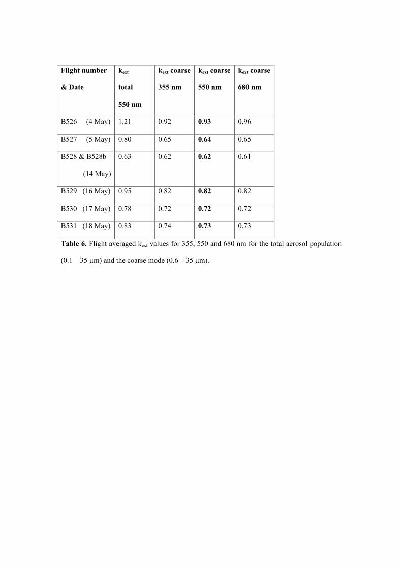
Flight number

& Date

kext

total

550 nm

kext coarse

355 nm

kext coarse

550 nm

kext coarse

680 nm

B526 (4 May) 1.21 0.92 0.93 0.96

B527 (5 May) 0.80 0.65 0.64 0.65

B528 & B528b

(14 May)

0.63 0.62 0.62 0.61

B529 (16 May) 0.95 0.82 0.82 0.82

B530 (17 May) 0.78 0.72 0.72 0.72

B531 (18 May) 0.83 0.74 0.73 0.73

Table 6. Flight averaged kext values for 355, 550 and 680 nm for the total aerosol population

(0.1 – 35 µm) and the coarse mode (0.6 – 35 µm).

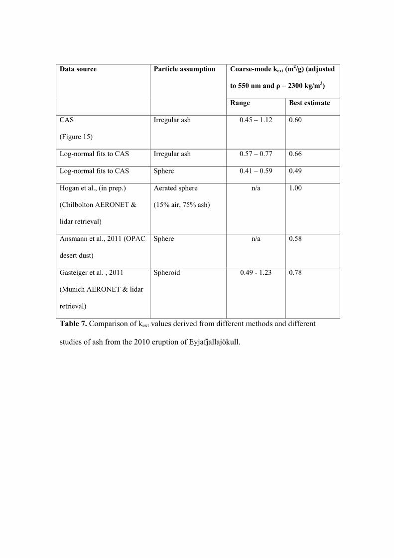
Coarse-mode kext (m2/g) (adjusted

to 550 nm and ρ = 2300 kg/m3)

Data source Particle assumption

Range Best estimate

CAS

(Figure 15)

Irregular ash 0.45 – 1.12 0.60

Log-normal fits to CAS Irregular ash 0.57 – 0.77 0.66

Log-normal fits to CAS Sphere 0.41 – 0.59 0.49

Hogan et al., (in prep.)

(Chilbolton AERONET &

lidar retrieval)

Aerated sphere

(15% air, 75% ash)

n/a 1.00

Ansmann et al., 2011 (OPAC

desert dust)

Sphere n/a 0.58

Gasteiger et al. , 2011

(Munich AERONET & lidar

retrieval)

Spheroid 0.49 - 1.23 0.78

Table 7. Comparison of kext values derived from different methods and different

studies of ash from the 2010 eruption of Eyjafjallajökull.