in search of the low volatility anomaly: a case study · pdf filein search of the low...

RESEARCH

Smart Beta

CONTRIBUTORS

Fei Mei Chan

Director

Index Investment Strategy

[email protected]

Craig J. Lazzara, CFA

Managing Director,

Global Head of


[email protected]

In Search of the Low Volatility

Anomaly: A Case Study

“There is nothing more deceptive than an obvious fact.”

- Sir Arthur Conan Doyle, “The Boscombe Valley Mystery”

EXECUTIVE SUMMARY

We introduce a simple analytic toolkit to assess the performance of

factor indices compared to their cap-weighted parents. The

methodology attributes a factor index’s excess returns to its

incremental (or decremental) level of risk and to a changed tradeoff

between risk and return.

The low volatility "anomaly,” as defined by an improved tradeoff

between risk and return, not only exists, but has strengthened in the

past six years.

More broadly, this toolkit can be used to assess the existence and

persistence of any factor-based effect.

Classical economic theory tells us that risk and return are directly related—

in general, in order to earn above-average returns an investor must be

prepared to bear above-average risks. Empirically, however, this

relationship does not hold; ample research and evidence point to the

existence of a low volatility factor comparable to other factors such as beta,

small size, or cheap valuation.1 Because this seems to fly in the face of

what we think we know about risk and return, the low volatility factor is

often referred to as the low volatility anomaly.

Exhibit 1 shows that the S&P 500® Low Volatility Index2 (including

backtested history) outperformed its parent S&P 500 between 1991 and

2015, despite exhibiting lower risk.

1 Jensen, Michael C., Fischer Black, and Myron S. Scholes, “The Capital Asset Pricing Model: Some Empirical Tests,” Studies in the Theory

of Capital Markets, Praeger Publishers Inc., 1972; Haugen, Robert A. and A. James Heines, “Risk and the Rate of Return on Financial Assets: Some Old Wine in New Bottles,” Journal of Financial and Quantitative Analysis, December 1975; Baker, Malcolm, Brendan Bradley, and Jeffrey Wurgler, “Benchmarks as Limits to Arbitrage: Understanding the Low-Volatility Anomaly,’ Financial Analysts Journal, January/February 2011.

2 The S&P 500 Low Volatility Index is designed to reflect the performance of the 100 stocks in the S&P 500 with the lowest historical standard deviation of returns.

mailto:[email protected]


https://www.spindices.com/indices/strategy/sp-500-low-volatility-index

http://us.spindices.com/indices/strategy/sp-500-low-volatility-index

In Search of the Low Volatility Anomaly: A Case Study April 2016

RESEARCH | Smart Beta 2

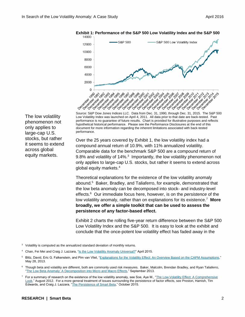
Exhibit 1: Performance of the S&P 500 Low Volatility Index and the S&P 500

Source: S&P Dow Jones Indices LLC. Data from Dec. 31, 1990, through Dec. 31, 2015. The S&P 500 Low Volatility Index was launched on April 4, 2011. All data prior to that date are back-tested. Past performance is no guarantee of future results. Chart is provided for illustrative purposes and reflects hypothetical historical performance. Please see the Performance Disclosures at the end of this document for more information regarding the inherent limitations associated with back-tested performance.

Over the 25 years covered by Exhibit 1, the low volatility index had a

compound annual return of 10.9%, with 11% annualized volatility.

Comparable data for the benchmark S&P 500 are a compound return of

9.8% and volatility of 14%.3 Importantly, the low volatility phenomenon not

only applies to large-cap U.S. stocks, but rather it seems to extend across

global equity markets.4

Theoretical explanations for the existence of the low volatility anomaly

abound.5 Baker, Bradley, and Taliaferro, for example, demonstrated that

the low beta anomaly can be decomposed into stock- and industry-level

effects.6 Our immediate focus here, however, is on the persistence of the

low volatility anomaly, rather than on explanations for its existence.7 More

broadly, we offer a simple toolkit that can be used to assess the

persistence of any factor-based effect.

Exhibit 2 charts the rolling five-year return difference between the S&P 500

Low Volatility Index and the S&P 500. It is easy to look at the exhibit and

conclude that the once-potent low volatility effect has faded away in the

3 Volatility is computed as the annualized standard deviation of monthly returns.

4 Chan, Fei Mei and Craig J. Lazzara, “Is the Low Volatility Anomaly Universal?” April 2015.

5 Blitz, David, Eric G. Falkenstein, and Pim van Vliet, “Explanations for the Volatility Effect: An Overview Based on the CAPM Assumptions,” May 28, 2013.

6 Though beta and volatility are different, both are commonly used risk measures. Baker, Malcolm, Brendan Bradley, and Ryan Taliaferro, “The Low Beta Anomaly: A Decomposition into Micro and Macro Effects,” September 2013.

7 For a summary of research on the existence of the low volatility anomaly, see Soe, Aye M., “The Low-Volatility Effect: A Comprehensive Look,” August 2012. For a more general treatment of issues surrounding the persistence of factor effects, see Preston, Hamish, Tim Edwards, and Craig J. Lazzara, “The Persistence of Smart Beta,” October 2015.

The low volatility phenomenon not only applies to large-cap U.S. stocks, but rather it seems to extend across global equity markets.



http://spindices.com/documents/research/research-is-the-low-volatility-anomaly-universal.pdf

https://papers.ssrn.com/sol3/papers.cfm?abstract_id=2270973

http://www.hbs.edu/faculty/Publication%20Files/FINAL%20Decomposition%20of%20Low%20Risk_36c1e488-c814-496a-bd3b-113e54b3be1d.pdf

http://spindices.com/documents/research/low-volatility-effect-comprehensive-look-201208.pdf

http://spindices.com/documents/research/low-volatility-effect-comprehensive-look-201208.pdf

http://spindices.com/documents/research/research-the-persistence-of-smart-beta.pdf



past few years. Since early 2013, the performance spread has drifted

around zero. Does this mean that the low volatility anomaly has

disappeared?

Exhibit 2: 5-Year Rolling Geometric Mean Difference (S&P 500 Low Volatility Index Versus the S&P 500)

Source: S&P Dow Jones Indices LLC. Data from Dec. 31, 1990, through Dec. 31, 2015. The S&P 500 Low Volatility Index was launched on April 4, 2011. All data prior to that date are back-tested. Past performance is no guarantee of future results. It is not possible to invest directly in an index, and index returns do not reflect expenses an investor would pay. Chart is provided for illustrative purposes and reflects hypothetical historical performance. Please see the Performance Disclosures at the end of this document for more information regarding the inherent limitations associated with back-tested performance.

PEELING THE ONION

Volatility Drag

One can, of course, attempt to address this question with a detailed factor

analysis.8 Here we will apply a simpler approach, based on the view that

we can analyze the difference between any two indices in terms of two

variables: the differences in the portfolios’ risk levels and the differences in

the ratio of return to risk. Risk adjustment is important generally9, and

nowhere more so than in considering strategies like low volatility, for which

reduced risk exposure is an integral part of the index’s definition.

An obvious first step in analyzing the impact of differential risk is to

remember that the arithmetic of compounding favors less-volatile return

patterns. Consider the hypothetical return patterns described in Exhibit 3.

8 See, e.g., Kang, Xiaowei, “Evaluating Alternate Beta Strategies,” February 2012.

9 See Preston, Edwards, and Lazzara, op. cit., pp. 8-10.

Risk adjustment is important generally nowhere more so than in considering strategies like low volatility.

http://spindices.com/documents/research/research-evaluating-alternate-beta-strategies.pdf



Exhibit 3: Illustration of Volatility Drag

PERIOD 1 (%) PERIOD 2 (%) COMPOUND RETURN (%) GEOMETRIC MEAN (%)

1 -1 -0.01 -0.003

5 -5 -0.25 -0.125

10 -10 -1.00 -0.501

15 -15 -2.25 -1.131

20 -20 -4.00 -2.020

25 -25 -6.25 -3.175

30 -30 -9.00 -4.606

35 -35 -12.25 -6.325

40 -40 -16.00 -8.348

45 -45 -20.25 -10.697

50 -50 -25.00 -13.397

Source: S&P Dow Jones Indices LLC. Table is provided for illustrative purposes and reflects hypothetical performance.

In each case, the expected return is 0%, since the results for period 1 and

period 2 offset each other.10 However, there is a notable difference

between increasing, and then declining, 1%, relative to increasing, and then

declining, 50%. The end result depends on the compounding of each

period’s return, and Exhibit 3 shows us that the compound return (and

geometric mean return) decline as the pattern of returns becomes more

volatile. Therefore volatility drag—i.e., the difference between the

geometric and arithmetic average returns—grows as volatility increases.

Since a low volatility index is, by design, less volatile than its parent, its

performance should be advantaged by lower volatility drag.

We can express these concepts algebraically by defining the following

terms.

Expected return = arithmetic mean = AM

Compound periodic return = geometric mean = GM

Volatility drag = VD = GM – AM

Using subscript p for a portfolio (e.g., a low volatility index) and subscript b

for a benchmark (e.g., the cap-weighted index from which the low volatility

index draws its constituents) lets us separate the volatility drag from the

differences in expected returns.

Compound return difference = GMp – GMb

= (AMp + VDp) – (AMb + VDb)

= (AMp – AMb) + (VDp – VDb)

10 We compute the expected return by taking the arithmetic mean of both periods’ results.

We can think about return along two dimensions: the amount of risk borne and the tradeoff between risk and return.



So the difference in compound average returns (as shown in Exhibit 2) is

accounted for by the difference in expected returns plus the difference

in volatility drag.

Expected Returns

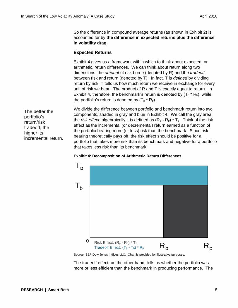
Exhibit 4 gives us a framework within which to think about expected, or

arithmetic, return differences. We can think about return along two

dimensions: the amount of risk borne (denoted by R) and the tradeoff

between risk and return (denoted by T). In fact, T is defined by dividing

return by risk; T tells us how much return we receive in exchange for every

unit of risk we bear. The product of R and T is exactly equal to return. In

Exhibit 4, therefore, the benchmark’s return is denoted by (Tb * Rb), while

the portfolio’s return is denoted by (Tp * Rp).

We divide the difference between portfolio and benchmark return into two

components, shaded in gray and blue in Exhibit 4. We call the gray area

the risk effect; algebraically it is defined as (Rp - Rb) * Tb. Think of the risk

effect as the incremental (or decremental) return earned as a function of

the portfolio bearing more (or less) risk than the benchmark. Since risk

bearing theoretically pays off, the risk effect should be positive for a

portfolio that takes more risk than its benchmark and negative for a portfolio

that takes less risk than its benchmark.

Exhibit 4: Decomposition of Arithmetic Return Differences

Source: S&P Dow Jones Indices LLC. Chart is provided for illustrative purposes.

The tradeoff effect, on the other hand, tells us whether the portfolio was

more or less efficient than the benchmark in producing performance. The

0

Tp

Tb

RpRbRisk Effect: (Rp - Rb) * Tb

Tradeoff Effect: (Tp - Tb) * Rp

The better the portfolio’s return/risk tradeoff, the higher its incremental return.



better the portfolio’s return/risk tradeoff, in other words, the higher its

incremental return.11

The difference between portfolio and benchmark returns can thus be

divided into three components.

1. The change in volatility drag, which should favor lower-risk strategies.

2. The change in return commensurate with changing risk. This should

favor higher-risk strategies most of the time, since there is typically a

positive reward for bearing risk. Combining this risk effect with the

change in volatility drag lets us calculate a total risk effect.

3. The change in the return/risk tradeoff, which can be either positive or

negative. If there is an anomaly to be found, this is where it is

likely to reside.

Cumulative Performance

Exhibit 5 illustrates the application of these principles over the entire period

for which return data exist for the S&P 500 Low Volatility Index. Our

observations include the following.

The difference in geometric means between the S&P 500 Low

Volatility Index and the S&P 500 is 0.083% per month. This seems

like a small difference, but the cumulative return over 25 years for the

S&P 500 Low Volatility Index amounts to 1331%, versus 1040% for

the S&P 500.12

The difference in arithmetic means (i.e., simple average monthly

returns) between the two indices was 0.046% per month, while the

difference in volatility drag was 0.037% per month. So at first blush, it

appears that about one-half of the performance advantage of low

volatility resulted simply because the low vol strategy was less

volatile.

But that first impression may be misleading. It is inaccurate to

conclude that low volatility is mainly a risk reduction story, for the

reasons shown in Exhibit 5. The low volatility strategy’s lower

volatility may be a double-edged sword. There was a positive

return for bearing risk in the 1991-2015 interval. The S&P 500 Low

Volatility Index’s return was reduced by 0.205% per month since it

bore less risk than the S&P 500. Adding this effect to the impact of

volatility drag means that the low volatility strategy’s reduced volatility

cost the index an average of 0.168% per month.

11 We acknowledge some ambiguity in constructing Exhibit 4, since the space at the upper right of the chart, which we assigned to the tradeoff

effect, could arguably be a risk effect, or a separate interaction effect. Algebraically, the value of the ambiguity is (Rp – Rb) * (Tp – Tb). For a low volatility index, the first of these terms is definitionally negative and the second is empirically positive, so the product of the two is usually negative. This means that treating the ambiguity as part of the tradeoff effect reduces the measured tradeoff effect below what it would otherwise be. We err, in other words, in the direction of conservatism.

12 This example is for illustrative purpose only.

It appears that about one-half of the performance advantage of the low volatility strategy came simply because it was less volatile, but that first impression may be misleading.




Countering the risk effects was the S&P 500 Low Volatility Index’s

improved reward for bearing risk. The S&P 500 produced 0.209 units

of return for every unit of risk, whereas the S&P 500 Low Volatility

Index’s return to risk ratio was an impressive 0.288. The impact of

this improved return to risk tradeoff resulted in an incremental

performance of 0.251% per month.

Arguably, this 0.251% per month is a measure of the low volatility

anomaly. Its existence is not a reward for risk bearing, which is accounted

for separately—and in any event, low volatility’s lower risk should not

require a return premium.

Exhibit 5: Sources of Monthly Relative Performance

REFERENCE FACTOR S&P 500 LOW

VOLATILITY INDEX (%) S&P 500 (%) DIFFERENCE (%)

A Geometric Mean 0.867 0.784 0.083

B Arithmetic Mean 0.918 0.871 0.046

C Volatility Drag (A-B) -0.051 -0.088 0.037

D Standard Deviation 3.187 4.168 -

E Reward for Risk (B/D) 0.288 0.209 -

F Impact of Changed Risk Level ((Dp-Db)*Eb)

- - -0.205

G Impact of Improved Tradeoff ((Ep-Eb)*Dp)

- - 0.251

H Difference in Arithmetic Means (F+G)

- - 0.046

I Sum of Risk Effects (C+F)

- - -0.168

J Improved Tradeoff, Arguably an Anomaly (G)

- - 0.251

K Difference in Geometric Means (I+J)

- - 0.083

Source: S&P Dow Jones Indices LLC. Data from Dec. 31, 1990, through Dec. 31, 2015. The S&P 500 Low Volatility Index was launched on April 4, 2011. All data prior to that date are back-tested. Past performance is no guarantee of future results. Table is provided for illustrative purposes and reflects hypothetical historical performance. Please see the Performance Disclosures at the end of this document for more information regarding the inherent limitations associated with back-tested performance.

DECOMPOSITION OVER TIME

Exhibit 5 is an overview of 25 years of index history. To understand

whether the putative low volatility anomaly is increasing or (as Exhibit 2

suggests) decreasing, we need to look at how the components of return

have evolved through time. We will use a rolling five-year window, just as

in Exhibit 2.

Exhibit 6 shows the evolution of volatility drag and the impact of changed

risk (rows C and F in Exhibit 5). The S&P 500 Low Volatility Index’s returns

have (unsurprisingly) consistently benefited from reduced volatility drag, but

they have typically been reduced because the portfolio assumes less risk

than its benchmark. More often than not, the sum of these risk effects was

The S&P 500 Low Volatility Index’s returns have (unsurprisingly) consistently benefited from reduced volatility drag.




negative—for most of the period measured in Exhibit 6, there was a positive

reward for risk bearing, and the reduction in return from taking on less risk

typically swamped the benefits of lower volatility drag.

Exhibit 6: Impact of Volatility Drag and Changed Risk

Source: S&P Dow Jones Indices LLC. Data from Dec. 31, 1990, to Dec. 31, 2015. The S&P 500 Low Volatility Index was launched on April 4, 2011. All data prior to that date are back-tested. Past performance is no guarantee of future results. Chart is provided for illustrative purposes and reflects hypothetical historical performance. Please see the Performance Disclosures at the end of this document for more information regarding the inherent limitations associated with back-tested performance.

This is more clearly seen in Exhibit 7, which combines the two effects

shown in Exhibit 6. If this were the extent of the low volatility story, there

would be no challenge to market efficiency and no academic discussion of

a possible anomaly, since the S&P 500 Low Volatility Index’s lower risk

was a performance drag most of the time.

Exhibit 7: Overall Risk Effect


The tradeoff effect contributed to the S&P 500 Low Volatility Index’s underperformance during the inflation of the technology bubble in 1997-1999.




THE TRADEOFF EFFECT

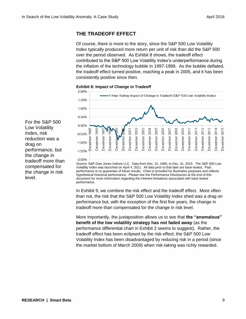
Of course, there is more to the story, since the S&P 500 Low Volatility

Index typically produced more return per unit of risk than did the S&P 500

over the period observed. As Exhibit 8 shows, the tradeoff effect

contributed to the S&P 500 Low Volatility Index’s underperformance during

the inflation of the technology bubble in 1997-1999. As the bubble deflated,

the tradeoff effect turned positive, reaching a peak in 2005, and it has been

consistently positive since then.

Exhibit 8: Impact of Change in Tradeoff


In Exhibit 9, we combine the risk effect and the tradeoff effect. More often

than not, the risk that the S&P 500 Low Volatility Index shed was a drag on

performance but, with the exception of the first five years, the change in

tradeoff more than compensated for the change in risk level.

More importantly, the juxtaposition allows us to see that the “anomalous”

benefit of the low volatility strategy has not faded away (as the

performance differential chart in Exhibit 2 seems to suggest). Rather, the

tradeoff effect has been eclipsed by the risk effect; the S&P 500 Low

Volatility Index has been disadvantaged by reducing risk in a period (since

the market bottom of March 2009) when risk-taking was richly rewarded.

For the S&P 500 Low Volatility Index, risk reduction was a drag on performance, but the change in tradeoff more than compensated for the change in risk level.




Exhibit 9: Risk Effect and Impact of Change in Tradeoff


However, there is another element to consider when analyzing factor

indices. The performance differential between any factor index and its

parent is conditioned by market dispersion, which is a measure of the

opportunity available to investors.13 When dispersion is relatively wide, the

opportunities to profit from stock selection are relatively large; when

dispersion is narrow, the opportunities diminish. Historically, S&P 500

dispersion peaked during the deflation of the technology bubble and during

the 2008 financial crisis (see Exhibit 10). Otherwise, dispersion has mostly

hovered between 4% and 8%.

Exhibit 10: S&P 500 Dispersion

Source: S&P Dow Jones Indices LLC. Data from Dec. 31, 1990, to Dec. 31, 2015. Past performance is no guarantee of future results. Chart is provided for illustrative purposes.

13 Chan, Fei Mei and Craig J. Lazzara, “Gauging Differential Returns,” January 2014. See also Edwards, Tim and Craig J. Lazzara,

“Dispersion: Measuring Market Opportunity,” December 2013.

When dispersion is relatively wide, the opportunities to profit from stock selection are relatively large; when dispersion is narrow, the opportunities diminish.

http://spindices.com/documents/research/research-gauging-differential-returns.pdf

http://spindices.com/documents/research/research-dispersion-measuring-market-opportunity.pdf



Over the past few years, dispersion has lingered near record low levels;

i.e., opportunity has been relatively limited. If we adjust the S&P 500 Low

Volatility Index’s tradeoff to account for the dispersion environment, the

effect is even greater.14 As Exhibit 11 shows, after adjusting for dispersion

levels, the tradeoff effect has been generally higher over the past two years

than during the 2008 peak. To the degree that we can identify the low

volatility anomaly with the low volatility strategy’s improved tradeoff

between risk and return, it is alive and well.

Exhibit 11: Impact of Change in Tradeoff (Adjusted for Dispersion)


PEELING MORE ONIONS

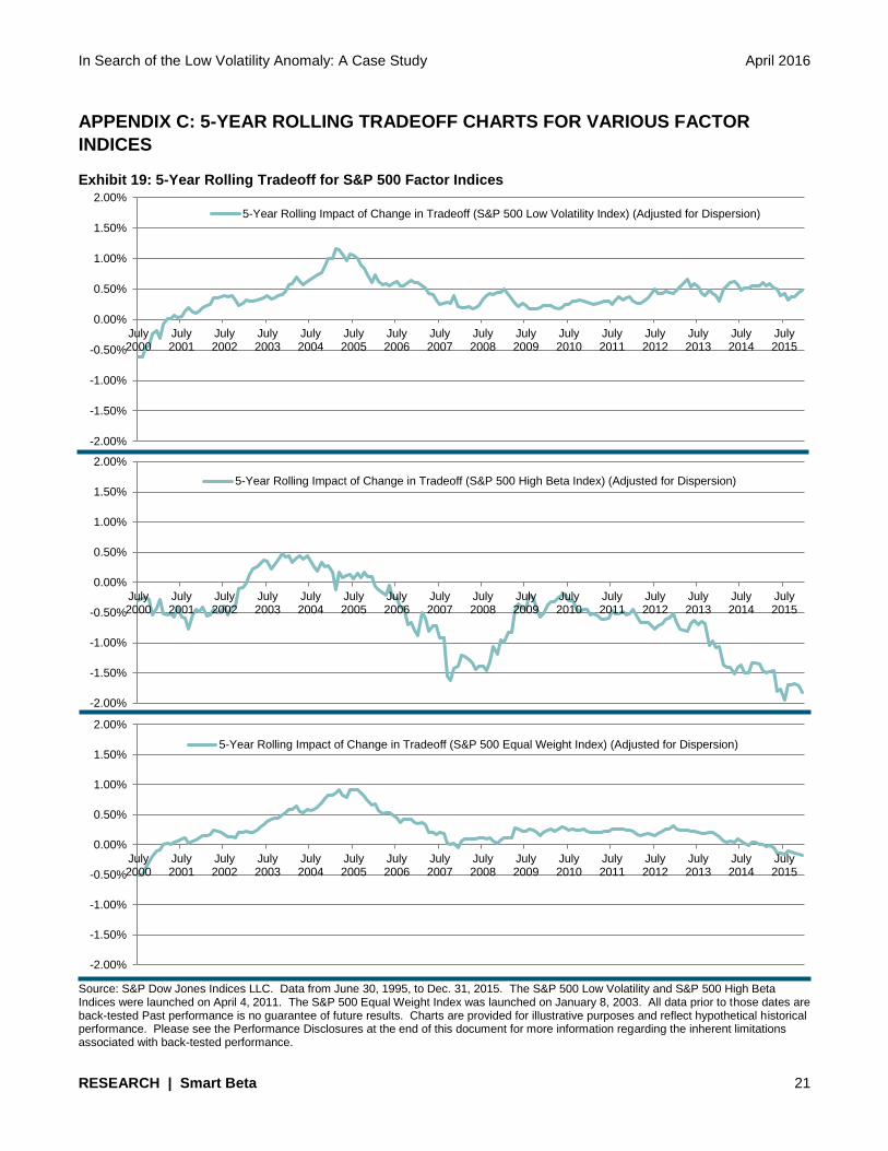
There is nothing about this analytic process that is unique to low

volatility indices. Exhibit 12, for example, shows the dispersion-adjusted

tradeoff for both the S&P 500 Low Volatility Index and its disparate

counterpart, the S&P 500 High Beta Index.15 Generally speaking, the S&P

500 High Beta Index’s tradeoff has been negative, and since the market

bottom of 2009, the high beta strategy’s tradeoff has become more

negative even as the low volatility strategy’s has improved. Given the close

relationship between beta and total volatility, the negative values for the

S&P 500 High Beta Index provide additional confirmation of the persistence

of the low volatility effect.

14 The adjustment is simple; we simply divide each month’s tradeoff by a scaled measure of the S&P 500’s dispersion.

15 The S&P 500 High Beta Index is designed to reflect the performance of the 100 stocks in the S&P 500 with the highest systematic risk.

The negative tradeoff for the S&P 500 High Beta Index provides additional confirmation of the persistence of the low volatility effect.




http://spindices.com/indices/strategy/sp-500-high-beta-index



Exhibit 12: Change in Tradeoff Effect for Two Disparate Factor Indices

Source: S&P Dow Jones Indices LLC. Data from Dec. 31, 1990, to Dec. 31, 2015. The S&P 500 Low Volatility and the S&P 500 High Beta Indices were launched on April 4, 2011. All data prior to that date are back-tested. Past performance is no guarantee of future results. Chart is provided for illustrative purposes and reflects hypothetical historical performance. Please see the Performance Disclosures at the end of this document for more information regarding the inherent limitations associated with back-tested performance.

Exhibit 13 shows the tradeoff for two other defensive strategy indices that

are also subsets of the S&P 500, the S&P 500 Dividend Aristocrats and the

S&P 500 Low Volatility High Dividend Index.16 Remarkably, given the

major differences in index methodologies, the tradeoff patterns in Exhibit 13

are so similar that they practically track one another.

Exhibit 13: Change in Tradeoff for Defensive Indices

Source: S&P Dow Jones Indices LLC. Data from Dec. 31, 1990, to Dec. 31, 2015. The S&P 500 Low Volatility was launched on April 4, 2011. The S&P 500 Dividend Aristocrats was launched on May 2, 2005. The S&P 500 Low Volatility High Dividend Index was launched on September 17, 2012. All data prior to those dates are back-tested. Past performance is no guarantee of future results. Chart is provided for illustrative purposes and reflects hypothetical historical performance. Please see the Performance Disclosures at the end of this document for more information regarding the inherent limitations associated with back-tested performance.

16 The S&P 500 Dividend Aristocrats Index is designed to measure the performance of S&P 500 members that have increased dividends for at

least the last 25 consecutive years. The S&P 500 Low Volatility High Dividend Index is designed to measure the performance of the 50 least-volatile high dividend-yielding stocks in the S&P 500.

Despite major differences in their methodologies, the tradeoff patterns of the S&P 500 Low Volatility Index, S&P 500 Dividend Aristocrats, and S&P 500 Low Volatility High Dividend Index are so similar that they practically track one another.

http://spindices.com/indices/strategy/sp-500-dividend-aristocrats

http://spindices.com/indices/strategy/sp-500-low-volatility-high-dividend-index



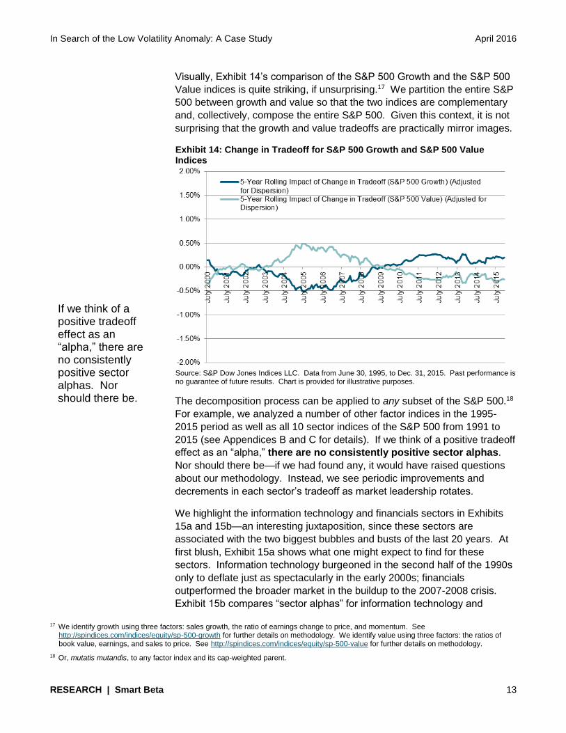
Visually, Exhibit 14’s comparison of the S&P 500 Growth and the S&P 500

Value indices is quite striking, if unsurprising.17 We partition the entire S&P

500 between growth and value so that the two indices are complementary

and, collectively, compose the entire S&P 500. Given this context, it is not

surprising that the growth and value tradeoffs are practically mirror images.

Exhibit 14: Change in Tradeoff for S&P 500 Growth and S&P 500 Value Indices

Source: S&P Dow Jones Indices LLC. Data from June 30, 1995, to Dec. 31, 2015. Past performance is no guarantee of future results. Chart is provided for illustrative purposes.

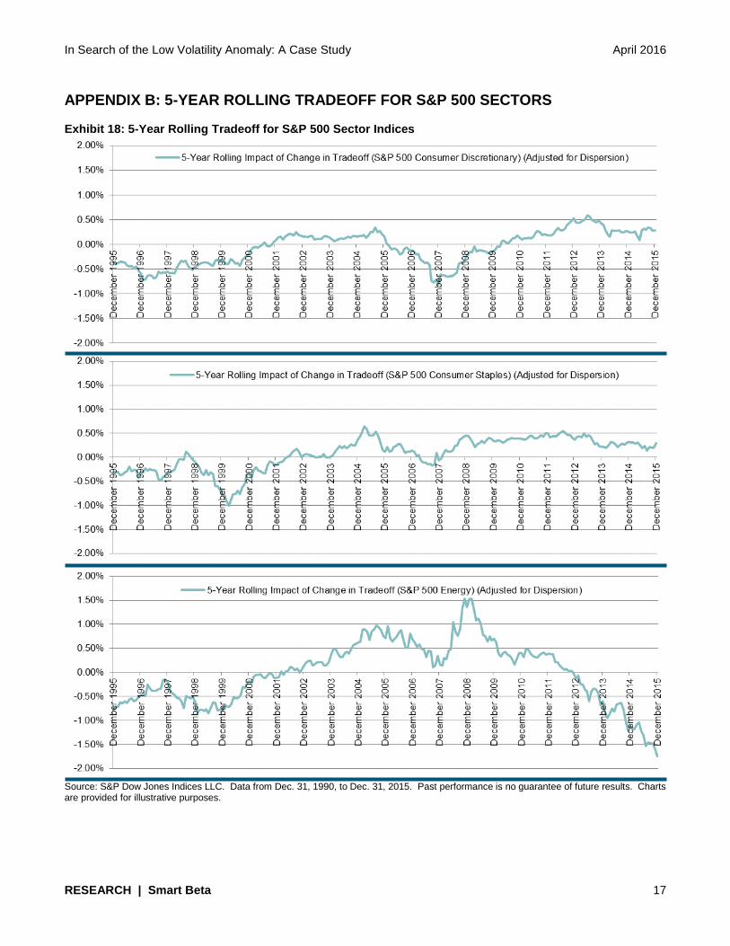
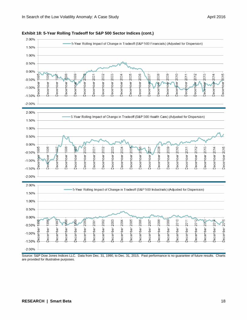
The decomposition process can be applied to any subset of the S&P 500.18

For example, we analyzed a number of other factor indices in the 1995-

2015 period as well as all 10 sector indices of the S&P 500 from 1991 to

2015 (see Appendices B and C for details). If we think of a positive tradeoff

effect as an “alpha,” there are no consistently positive sector alphas.

Nor should there be—if we had found any, it would have raised questions

about our methodology. Instead, we see periodic improvements and

decrements in each sector’s tradeoff as market leadership rotates.

We highlight the information technology and financials sectors in Exhibits

15a and 15b—an interesting juxtaposition, since these sectors are

associated with the two biggest bubbles and busts of the last 20 years. At

first blush, Exhibit 15a shows what one might expect to find for these

sectors. Information technology burgeoned in the second half of the 1990s

only to deflate just as spectacularly in the early 2000s; financials

outperformed the broader market in the buildup to the 2007-2008 crisis.

Exhibit 15b compares “sector alphas” for information technology and

17 We identify growth using three factors: sales growth, the ratio of earnings change to price, and momentum. See

http://spindices.com/indices/equity/sp-500-growth for further details on methodology. We identify value using three factors: the ratios of book value, earnings, and sales to price. See http://spindices.com/indices/equity/sp-500-value for further details on methodology.

18 Or, mutatis mutandis, to any factor index and its cap-weighted parent.

If we think of a positive tradeoff effect as an “alpha,” there are no consistently positive sector alphas. Nor should there be.

http://spindices.com/indices/equity/sp-500-growth

http://spindices.com/indices/equity/sp-500-value



financials, which shows that their similarities may have been more

superficial than real.

Even in 2000, at the height of the tech bubble, information

technology’s “sector alpha” was negligible. This implies that the

exceptional returns of the information technology sector in its

glory years were a function of the sector’s exceptionally high

volatility levels.

The financials sector, on the other hand, showed substantial positive

“alpha” in the early 2000s (and has shown substantial negative

“alpha” since 2007). The sector’s apparent idiosyncratic

performance, in other words, appears to have been truly

idiosyncratic.

Exhibit 15a: Performance Differential for S&P 500 Financials and Information Technology Sectors


Exhibit 15b: Tradeoff for S&P 500 Financials and Information Technology Sectors


We found that the S&P 500 Low Volatility Index’s recent performance challenges are attributable to its reduced level of risk in an environment that, until recently, has been favorable for risk-taking.



CONCLUSION

We have presented a simple methodology that can be used to assess the

performance of factor (or other) indices compared to their cap-weighted

parents. The methodology attributes a factor index’s return differential both

to its incremental (or decremental) level of risk and to a changed tradeoff

between risk and return. In the particular case of the S&P 500 Low

Volatility Index, our analysis indicates that its recent performance

challenges are attributable to its reduced level of risk in an environment

that, until recently, has been favorable for risk-taking. The S&P 500 Low

Volatility Index’s improved tradeoff between risk and return, which is

arguably the source of its anomalous performance, has remained

intact.





APPENDIX A: APPLES TO APPLES

The S&P 500 Low Volatility Index is much closer to being equal-weighted than cap-weighted, which

makes it arguable that the S&P 500 Equal Weight Index is a more appropriate benchmark for the low

volatility strategy than is the cap-weighted S&P 500.19 Rescaling Exhibit 5 using the S&P 500 Equal

Weight Index as the benchmark is also worthwhile because in the period from 1991 to 2015, the S&P

500 Low Volatility Index underperformed the S&P 500 Equal Weight Index by a monthly average of

7.7 bps. Here, the tradeoff effect remains significant and positive, but the low volatility strategy’s

reduced risk was a burden for which the improved tradeoff could not compensate. Detecting the low

volatility anomaly, in other words, does not depend on using the cap-weighted S&P 500 as a

benchmark.

Exhibit 16: Sources of Relative Performance

REFERENCE FACTOR S&P 500 LOW

VOLATILITY INDEX (%) S&P 500 EQUAL

WEIGHT INDEX (%) DIFFERENCE (%)

A Geometric Mean 0.867 0.994 -0.077

B Arithmetic Mean 0.918 1.051 -0.134

C Volatility Drag (A-B) -0.051 -0.107 0.057

D Standard Deviation 3.19 4.62 -

E Reward for Risk (B/D) 0.288 0.227 -

F Impact of Changed Risk Level ((Dp-Db)*Eb) - - -0.326

G Impact of Improved Tradeoff ((Ep-Eb)*Dp) - - 0.193

H Difference in Arithmetic Means (F+G) - - -0.134

I Sum of Risk Effects (C+F) - - -0.270

J Improved Tradeoff, Arguably an Anomaly (G) - - 0.193

K Difference in Geometric Means (I+J) - - -0.077

Source: S&P Dow Jones Indices LLC. Data from Dec. 31, 1990, through Dec. 31, 2015. The S&P 500 Low Volatility Index was launched on April 4, 2011. The S&P 500 Equal Weight Index was launched on January 8, 2003. All data prior to those dates are back-tested. Past performance is no guarantee of future results. Table is provided for illustrative purposes and reflects hypothetical historical performance. Please see the Performance Disclosures at the end of this document for more information regarding the inherent limitations associated with back-tested performance.

Exhibit 17: Impact of Change in Tradeoff (Adjusted for Dispersion)

Source: S&P Dow Jones Indices LLC. Data from Dec. 31, 1990, to Dec. 31, 2015. The S&P 500 Low Volatility Index was launched on April 4, 2011. All data prior to that date are back-tested. Past performance is no guarantee of future results. Chart is provided for illustrative purposes.

19 See Edwards, Tim and Craig J. Lazzara, “Equal-Weight Benchmarking: Raising the Monkey Bars,” June 2014.


http://spindices.com/documents/research/research-equal-weight-benchmarking-raising-the-monkey-bars.pdf



APPENDIX B: 5-YEAR ROLLING TRADEOFF FOR S&P 500 SECTORS

Exhibit 18: 5-Year Rolling Tradeoff for S&P 500 Sector Indices

Source: S&P Dow Jones Indices LLC. Data from Dec. 31, 1990, to Dec. 31, 2015. Past performance is no guarantee of future results. Charts are provided for illustrative purposes.



Exhibit 18: 5-Year Rolling Tradeoff for S&P 500 Sector Indices (cont.)




APPENDIX C: 5-YEAR ROLLING TRADEOFF CHARTS FOR VARIOUS FACTOR

INDICES

Exhibit 19: 5-Year Rolling Tradeoff for S&P 500 Factor Indices

Source: S&P Dow Jones Indices LLC. Data from June 30, 1995, to Dec. 31, 2015. The S&P 500 Low Volatility and S&P 500 High Beta Indices were launched on April 4, 2011. The S&P 500 Equal Weight Index was launched on January 8, 2003. All data prior to those dates are back-tested Past performance is no guarantee of future results. Charts are provided for illustrative purposes and reflect hypothetical historical performance. Please see the Performance Disclosures at the end of this document for more information regarding the inherent limitations associated with back-tested performance.

-2.00%

-1.50%

-1.00%

-0.50%

0.00%

0.50%

1.00%

1.50%

2.00%

July2000

July2001

July2002

July2003

July2004

July2005

July2006

July2007

July2008

July2009

July2010

July2011

July2012

July2013

July2014

July2015

5-Year Rolling Impact of Change in Tradeoff (S&P 500 Low Volatility Index) (Adjusted for Dispersion)

-2.00%

-1.50%

-1.00%

-0.50%

0.00%

0.50%

1.00%

1.50%

2.00%

July2000

July2001

July2002

July2003

July2004

July2005

July2006

July2007

July2008

July2009

July2010

July2011

July2012

July2013

July2014

July2015

5-Year Rolling Impact of Change in Tradeoff (S&P 500 High Beta Index) (Adjusted for Dispersion)

-2.00%

-1.50%

-1.00%

-0.50%

0.00%

0.50%

1.00%

1.50%

2.00%

July2000

July2001

July2002

July2003

July2004

July2005

July2006

July2007

July2008

July2009

July2010

July2011

July2012

July2013

July2014

July2015

5-Year Rolling Impact of Change in Tradeoff (S&P 500 Equal Weight Index) (Adjusted for Dispersion)



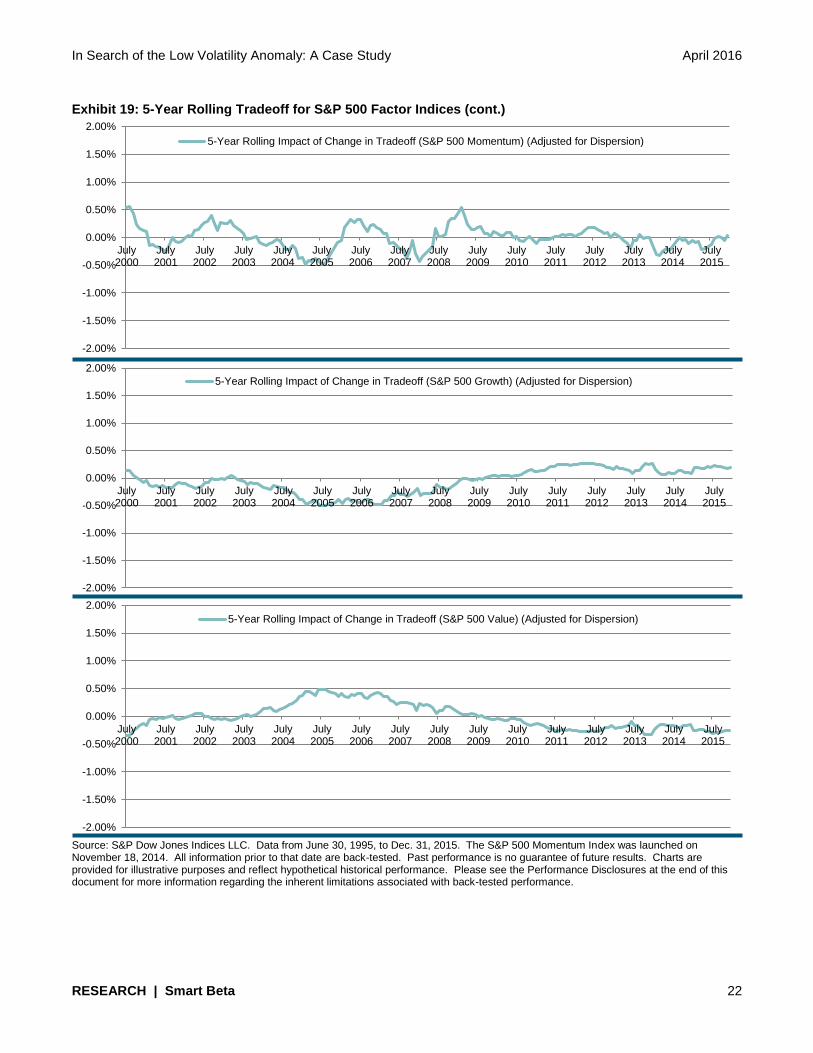
Exhibit 19: 5-Year Rolling Tradeoff for S&P 500 Factor Indices (cont.)

Source: S&P Dow Jones Indices LLC. Data from June 30, 1995, to Dec. 31, 2015. The S&P 500 Momentum Index was launched on November 18, 2014. All information prior to that date are back-tested. Past performance is no guarantee of future results. Charts are provided for illustrative purposes and reflect hypothetical historical performance. Please see the Performance Disclosures at the end of this document for more information regarding the inherent limitations associated with back-tested performance.

-2.00%

-1.50%

-1.00%

-0.50%

0.00%

0.50%

1.00%

1.50%

2.00%

July2000

July2001

July2002

July2003

July2004

July2005

July2006

July2007

July2008

July2009

July2010

July2011

July2012

July2013

July2014

July2015

5-Year Rolling Impact of Change in Tradeoff (S&P 500 Momentum) (Adjusted for Dispersion)

-2.00%

-1.50%

-1.00%

-0.50%

0.00%

0.50%

1.00%

1.50%

2.00%

July2000

July2001

July2002

July2003

July2004

July2005

July2006

July2007

July2008

July2009

July2010

July2011

July2012

July2013

July2014

July2015

5-Year Rolling Impact of Change in Tradeoff (S&P 500 Growth) (Adjusted for Dispersion)

-2.00%

-1.50%

-1.00%

-0.50%

0.00%

0.50%

1.00%

1.50%

2.00%

July2000

July2001

July2002

July2003

July2004

July2005

July2006

July2007

July2008

July2009

July2010

July2011

July2012

July2013

July2014

July2015

5-Year Rolling Impact of Change in Tradeoff (S&P 500 Value) (Adjusted for Dispersion)



Exhibit 19: 5-Year Rolling Tradeoff for S&P 500 Factor Indices (cont.)

Source: S&P Dow Jones Indices LLC. Data from June 30, 1995, to Dec. 31, 2015. The S&P 500 Pure Growth and the S&P 500 Pure Value Indices were launched on December 16, 2005. The S&P 500 Enhanced Value Index was launched on April 27, 2015. All data prior to those dates are back-tested. Past performance is no guarantee of future results. Charts are provided for illustrative purposes and reflect hypothetical historical performance. Please see the Performance Disclosures at the end of this document for more information regarding the inherent limitations associated with back-tested performance.

-2.00%

-1.50%

-1.00%

-0.50%

0.00%

0.50%

1.00%

1.50%

2.00%

July2000

July2001

July2002

July2003

July2004

July2005

July2006

July2007

July2008

July2009

July2010

July2011

July2012

July2013

July2014

July2015

5-Year Rolling Impact of Change in Tradeoff (S&P 500 Pure Growth) (Adjusted for Dispersion)

-2.00%

-1.50%

-1.00%

-0.50%

0.00%

0.50%

1.00%

1.50%

2.00%

July2000

July2001

July2002

July2003

July2004

July2005

July2006

July2007

July2008

July2009

July2010

July2011

July2012

July2013

July2014

July2015

5-Year Rolling Impact of Change in Tradeoff (S&P 500 Pure Value) (Adjusted for Dispersion)

-2.00%

-1.50%

-1.00%

-0.50%

0.00%

0.50%

1.00%

1.50%

2.00%

July2000

July2001

July2002

July2003

July2004

July2005

July2006

July2007

July2008

July2009

July2010

July2011

July2012

July2013

July2014

July2015

5-Year Rolling Impact of Change in Tradeoff (S&P 500 Enhanced Value Index) (Adjusted for Dispersion)



S&P DJI Research Contributors

NAME TITLE EMAIL

Charles “Chuck” Mounts Global Head [email protected]

Global Research & Design

Aye Soe, CFA Americas Head [email protected]

Dennis Badlyans Associate Director [email protected]

Phillip Brzenk, CFA Director [email protected]

Smita Chirputkar Director [email protected]

Rachel Du Senior Analyst [email protected]

Qing Li Associate Director [email protected]

Berlinda Liu, CFA Director [email protected]

Ryan Poirier Senior Analyst [email protected]

Maria Sanchez Associate Director [email protected]

Kelly Tang, CFA Director [email protected]

Peter Tsui Director [email protected]

Hong Xie, CFA Director [email protected]

Priscilla Luk APAC Head [email protected]

Utkarsh Agrawal Associate Director [email protected]

Liyu Zeng, CFA Director [email protected]

Sunjiv Mainie, CFA, CQF

EMEA Head [email protected]

Daniel Ung, CFA, CAIA, FRM

Director [email protected]

Andrew Innes Senior Analyst [email protected]


Craig Lazzara, CFA Global Head [email protected]

Fei Mei Chan Director [email protected]

Tim Edwards, PhD Senior Director [email protected]

Howard Silverblatt Senior Industry Analyst [email protected]









PERFORMANCE DISCLOSURE

The S&P 500 Low Volatility Index and the S&P 500 High Beta Index were launched on April 4, 2011. The S&P 500 Dividend Aristocrats was launched on May 2, 2005. The S&P 500 Low Volatility High Dividend Index was launched on September 17, 2012. The S&P 500 Pure Growth and the S&P 500 Pure Value were launched on December 16, 2005. The S&P 500 Equal Weight Index was launched on January 8, 2003. The S&P 500 Momentum was launched on November 18, 2014. The S&P 500 Enhanced Value Index was launched on April 27, 2015. All information presented prior to an index’s Launch Date is hypothetical (back-tested), not actual performance. The back-test calculations are based on the same methodology that was in effect on the index Launch Date. Complete index methodology details are available at www.spdji.com.

S&P Dow Jones Indices defines various dates to assist our clients in providing transparency. The First Value Date is the first day for which there is a calculated value (either live or back-tested) for a given index. The Base Date is the date at which the Index is set at a fixed value for calculation purposes. The Launch Date designates the date upon which the values of an index are first considered live: index values provided for any date or time period prior to the index’s Launch Date are considered back-tested. S&P Dow Jones Indices defines the Launch Date as the date by which the values of an index are known to have been released to the public, for example via the company’s public website or its datafeed to external parties. For Dow Jones-branded indices introduced prior to May 31, 2013, the Launch Date (which prior to May 31, 2013, was termed “Date of introduction”) is set at a date upon which no further changes were permitted to be made to the index methodology, but that may have been prior to the Index’s public release date.

Past performance of the Index is not an indication of future results. Prospective application of the methodology used to construct the Index may not result in performance commensurate with the back-test returns shown. The back-test period does not necessarily correspond to the entire available history of the Index. Please refer to the methodology paper for the Index, available at www.spdji.com for more details about the index, including the manner in which it is rebalanced, the timing of such rebalancing, criteria for additions and deletions, as well as all index calculations.

Another limitation of using back-tested information is that the back-tested calculation is generally prepared with the benefit of hindsight. Back-tested information reflects the application of the index methodology and selection of index constituents in hindsight. No hypothetical record can completely account for the impact of financial risk in actual trading. For example, there are numerous factors related to the equities, fixed income, or commodities markets in general which cannot be, and have not been accounted for in the preparation of the index information set forth, all of which can affect actual performance.

The Index returns shown do not represent the results of actual trading of investable assets/securities. S&P Dow Jones Indices LLC maintains the Index and calculates the Index levels and performance shown or discussed, but does not manage actual assets. Index returns do not reflect payment of any sales charges or fees an investor may pay to purchase the securities underlying the Index or investment funds that are intended to track the performance of the Index. The imposition of these fees and charges would cause actual and back-tested performance of the securities/fund to be lower than the Index performance shown. As a simple example, if an index returned 10% on a US $100,000 investment for a 12-month period (or US $10,000) and an actual asset-based fee of 1.5% was imposed at the end of the period on the investment plus accrued interest (or US $1,650), the net return would be 8.35% (or US $8,350) for the year. Over a three year period, an annual 1.5% fee taken at year end with an assumed 10% return per year would result in a cumulative gross return of 33.10%, a total fee of US $5,375, and a cumulative net return of 27.2% (or US $27,200).

http://www.spdji.com/

http://www.spdji.com/



GENERAL DISCLAIMER

Copyright © 2016 by S&P Dow Jones Indices LLC, a part of S&P Global. All rights reserved. Standard & Poor’s ®, S&P 500 ® and S&P ® are registered trademarks of Standard & Poor’s Financial Services LLC (“S&P”), a subsidiary of S&P Global. Dow Jones ® is a registered trademark of Dow Jones Trademark Holdings LLC (“Dow Jones”). Trademarks have been licensed to S&P Dow Jones Indices LLC. Redistribution, reproduction and/or photocopying in whole or in part are prohibited without written permission. This document does not constitute an offer of services in jurisdictions where S&P Dow Jones Indices LLC, Dow Jones, S&P or their respective affiliates (collectively “S&P Dow Jones Indices”) do not have the necessary licenses. All information provided by S&P Dow Jones Indices is impersonal and not tailored to the needs of any person, entity or group of persons. S&P Dow Jones Indices receives compensation in connection with licensing its indices to third parties. Past performance of an index is not a guarantee of future results.

It is not possible to invest directly in an index. Exposure to an asset class represented by an index is available through investable instruments based on that index. S&P Dow Jones Indices does not sponsor, endorse, sell, promote or manage any investment fund or other investment vehicle that is offered by third parties and that seeks to provide an investment return based on the performance of any index. S&P Dow Jones Indices makes no assurance that investment products based on the index will accurately track index performance or provide positive investment returns. S&P Dow Jones Indices LLC is not an investment advisor, and S&P Dow Jones Indices makes no representation regarding the advisability of investing in any such investment fund or other investment vehicle. A decision to invest in any such investment fund or other investment vehicle should not be made in reliance on any of the statements set forth in this document. Prospective investors are advised to make an investment in any such fund or other vehicle only after carefully considering the risks associated with investing in such funds, as detailed in an offering memorandum or similar document that is prepared by or on behalf of the issuer of the investment fund or other vehicle. Inclusion of a security within an index is not a recommendation by S&P Dow Jones Indices to buy, sell, or hold such security, nor is it considered to be investment advice.

These materials have been prepared solely for informational purposes based upon information generally available to the public and from sources believed to be reliable. No content contained in these materials (including index data, ratings, credit-related analyses and data, research, valuations, model, software or other application or output therefrom) or any part thereof (Content) may be modified, reverse-engineered, reproduced or distributed in any form or by any means, or stored in a database or retrieval system, without the prior written permission of S&P Dow Jones Indices. The Content shall not be used for any unlawful or unauthorized purposes. S&P Dow Jones Indices and its third-party data providers and licensors (collectively “S&P Dow Jones Indices Parties”) do not guarantee the accuracy, completeness, timeliness or availability of the Content. S&P Dow Jones Indices Parties are not responsible for any errors or omissions, regardless of the cause, for the results obtained from the use of the Content. THE CONTENT IS PROVIDED ON AN “AS IS” BASIS. S&P DOW JONES INDICES PARTIES DISCLAIM ANY AND ALL EXPRESS OR IMPLIED WARRANTIES, INCLUDING, BUT NOT LIMITED TO, ANY WARRANTIES OF MERCHANTABILITY OR FITNESS FOR A PARTICULAR PURPOSE OR USE, FREEDOM FROM BUGS, SOFTWARE ERRORS OR DEFECTS, THAT THE CONTENT’S FUNCTIONING WILL BE UNINTERRUPTED OR THAT THE CONTENT WILL OPERATE WITH ANY SOFTWARE OR HARDWARE CONFIGURATION. In no event shall S&P Dow Jones Indices Parties be liable to any party for any direct, indirect, incidental, exemplary, compensatory, punitive, special or consequential damages, costs, expenses, legal fees, or losses (including, without limitation, lost income or lost profits and opportunity costs) in connection with any use of the Content even if advised of the possibility of such damages.

S&P Dow Jones Indices keeps certain activities of its business units separate from each other in order to preserve the independence and objectivity of their respective activities. As a result, certain business units of S&P Dow Jones Indices may have information that is not available to other business units. S&P Dow Jones Indices has established policies and procedures to maintain the confidentiality of certain non-public information received in connection with each analytical process.

In addition, S&P Dow Jones Indices provides a wide range of services to, or relating to, many organizations, including issuers of securities, investment advisers, broker-dealers, investment banks, other financial institutions and financial intermediaries, and accordingly may receive fees or other economic benefits from those organizations, including organizations whose securities or services they may recommend, rate, include in model portfolios, evaluate or otherwise address.

in search of the low volatility anomaly: a case study · pdf filein search of the low...

Documents