in mathematical physics - uc davis mathematicstemple/!!!pubsforweb/cv33.pdfcommun. math. phys. 156,...
TRANSCRIPT
Commun. Math. Phys. 156, 67-99 (1993) Communications in" Mathematical
Physics �9 Springer-Verlag 1993
Global Solutions of the Relativistic Euler Equations
Joel Smoller 1, Blake Temple 2 1 Department of Mathematics, University of Michigan, Ann Arbor, MI 48109, USA; Supported in part by NSF Applied Mathematics Grant Number DMS-89-05205 2 Department of Mathematics, University of California, Davis, Davis CA 95616, USA, Supported in part by NSF Applied Mathematics Grant Number DMS-86-13450
Received April 24, 1992
Abstract. We demonstrate the existence of solutions with shocks for the equations describing a perfect fluid in special relativity, namely, d i v T = 0, where T ~ = (p + pcZ)ulU j + prl ij is the stress energy tensor for the fluid. Here, p denotes the pressure, u the 4-velocity, p the mass-energy density of the fluid, t/~ the flat Minkowski metric, and c the speed of light. We assume that the equation of state is given by p -- a2p, where o -2, the sound speed, is constant. For these equations, we construct bounded weak solutions of the initial value problem in two dimensional Minkowski spacetime, for any initial data of finite total variation. The analysis is based on showing that the total variation of the variable ln(p) is non-increasing on approximate weak solutions generated by Glimm's method, and so this quantity, unique to equations of this type, plays a role similar to an energy function. We also show that the weak solutions (p(x ~ x 1), v(x~ 1)) themselves satisfy the Lorentz
invariant estimates Var{ln(p(x~ < Vo and Var fln ~ + v (x~ _ v(xO,.)j < V1 for all t
x ~ > 0, where Vo and V~ are Lorentz invariant constants that depend only on the total variation of the initial data, and v is the classical velocity. The equation of state p = (c2/3)p describes a gas of highly relativistic particles in several important general relativistic models which describe the evolution of stars.
1. Introduction
We consider the relativistic equations for a perfect fluid in Minkowski spacetime,
div T = 0 , (1)
where
T ij = (p + p c Z ) u i u j -t- ptl ij (2)
denotes the stress-energy tensor for the fluid. Recall that in Minkowski spacetime,
div T - Tj, , , (3)

68 J. Smoller and B. Temple
where we use the Einstein summat ion convention and assume summat ion over repeated up-down indices. The nota t ion ", i" denotes differentiation with respect to the variable x i, and in general all indices run from 0 to 3 with x ~ =_ ct. In (2), c denotes the speed of light, p the pressure, u the 4-velocity of the fluid particle (the velocity of the frame of isotropy of the perfect fluid), p the mass-energy density of the fluid (as measured in units of mass in a reference frame moving with the fluid particle), and ~/iJ = qz~ - d i a g ( - 1, 1, 1, 1) denotes the flat Minkowski metric. In the case of a barotropic gas, p is given by an explicit function of p, and this defines the equat ion of state. Barotropic fluids are impor tant in the study of stellar evolution in general relativity. 3 In the case of barotropic flow, system (1) describes a system of four conservation laws in the four unknowns p and u. Recall that since u = (1/c)dx/d~, (T is the proper time, u is a unit four vector in Minkowsk.i space) it follows that (/,/0)2 __ ~31 (U~)2 = 1, and thus only three of the quantities u ~ . . . . , u 3 are independent.
As a special example of barotropic flow, the equat ion of state p = (c2/3)p arises in several impor tant relativistic settings. In particular, the equation of state p = (c2/3)p follows directly from the Stefan-Bol tzmann law when a gas is in thermo- dynamical equilibrium with radiation and the radiation energy density greatly exceeds the total gas energy density. Indeed, the significance of the special case p = (c2/3)p is further discussed in the following quote from the recent book of A.M. Anile [1], starting at the bo t tom of p. 12:
An example of astrophysical i n t e r e s t . . , is provided by a gas in local thermodynamical equilibrium with radiation when the radiation energy density greatly exceeds the total gas energy density. Since for radiation, one has [the S tephan-Bol tzmann law] p = CB T 4 and p = (1/3)C~ T 4 [where c = 1, T = temperature and CB denotes the S tephan-Bol tzmann constant] , when the radiation energy density dominates, the fluid obeys the equat ion of state p = (1/3)p . . . . Other examples are provided by a fluid of massless n e u t r i n o s . . , or a fluid of ultra-relativistic electron-positron pairs . . . . In both cases, the pressure is given by p = (1/3)p. It is interesting to notice that in the early universe, at sufficiently high temperatures, all the particles become relativistic. Therefore, the equat ion of state p = (1/3)p would [also] be applicable under these circumstances.
The equat ion of state p = (c2/3)p has also been impor tant in the study of gravitational collapse because it can be derived as a model for the equation of state in a dense Neut ron star. This derivation is given in Weinberg [20], p. 320. This
3 We quote Weinberg [20], p. 301 (Weinberg uses the term "isentropic" in place of"barotropic"):
[the assumption that the] star is isentropic is valid for two very different kinds of stars: (A) Stars at Absolute Zero. When a star exhausts its thermonuclear fuel it can become a white dwarf, or a neutron star, in which the temperature is essentially at absolute zero. According to Nernst's theorem, the entropy per nucleon will then be zero throughout the star. (B) Stars in Convective Equilibrium. If the most efficient mechanism for energy transfer within the star is convection, then in equilibrium the entropy per nucleon must be nearly constant throughout the star, because otherwise a small element of fluid.., could gain or lose energy when transported from one part of the star to another, and convection would therefore disturb the energy distribution. The supermassive stars are generally presumed to be in convective equilibrium . . . . The importance of these assumptions lies in the fact that the pressure p . . . may be regarded as a function of the energy density p alone
Globa l Solutions of the Relativistic Euler Equat ions 69
result is also discussed in the famous works of Oppenheimer and Snyder and Oppenheimer and Volkoff [14,15] on gravitational collapse; see also [6, 11, 18, 193.
The equation of state p = o-2p also describes the equation of state in isothermal flow. The isothermal case is valid in the early stages of stellar formation. If one imagines a slowly collapsing cloud of interstellar gas or dust particles, the collapse reaches a stage where the mean free path for photon transmission within the cloud becomes small enough so that the scattering of photons is a significant effect. During the period where the motion within the cloud remains relatively small, the photon scattering has the effect of equalizing the temperature throughout the cloud, and thus p -- a2p is valid. 4
Observe also that a general equation of state p = p(p) can be approximated by one of form (6) by linearizing the pressure about an arbitrary value of p, and that, moreover, an equation of state p = p(p) must become linear as p ~ ~ in order that the sound speed ~ not exceed the speed of light at large densities p (see Sect. 3).
In this paper we will analyze the case when the equation of state is given by p = a2p, where the sound speed a is assumed to be constant. (Note that a has the dimensions of velocity because we take p to have the dimensions of mass, not energy.) We note that, whereas in the classical regime the equation of state p = aZp can only be viewed as a model problem for fluid flow, in the relativistic regime, this equation of state is of fundamental importance. It is also interesting to note that the hyperbolic conservation laws (1) play a more basic role in relativistic fluids than in classical fluids because infinite speed of propagation, which is a property of parabolic type systems such as the Navier-Stokes equations, is ruled out at the start in this setting by the relativistic principle that all velocities are bounded by c.
We study here the initial value problem for (1) in a two dimensional spacetime (x ~ xl), so that p and u are unknown functions of (x ~ xl), and
tt 'J = 0 " (4 )
Under these assumptions the stress-energy tensor (2) takes the form
T ij = ~(P + PCZ)U~176 - P (P + PC2)U~ 1 (5 )
[_ (p -l- pC2)uOu 1 (p -4- pC2)UlU 1 -']- p J "
In one space and one time dimension, the system (1), div T = 0, provides a model for the dynamics of plane waves in special relativistic fluids.
For our theorem we assume that p and p satisfy an equation of state of the form
p = o '2p , (6)
where ~2, the sound speed, is taken to be constant, o-< c. In particular, when a 2 = c2/3, (6) gives the important relativistic case p = (c2/3)p discussed above. Since the background metric is the flat Minkowski metric t/ii, the increment of proper time z, (Minkowski arclength), along a curve is given by the formula
d(() 2 = - rlij dx i dx ~ , (7)
4 We thank D. Christodoulou for bringing this to our attention, [2]
70 J. Smoller and B. Temple
where we use the notation ~ = cr. In this way the coordinate time t and the proper time T have the dimensions of time, while x ~ and ~ have the dimensions of length. Since u = dxi/d(c~), (where differentiation is taken along a particle path), defines the dimensionless velocity of the fluid, we must have
uO ~__ N/1 + (U 1)2.
Thus letting u = u 1, the equations we consider are
Oxo{(p+pc2)(1 + u 2 ) - p } + { (p+pc2)ux /1 + u 2 ) = 0 ,
(8)
c3xO {(p + pc2)ux/1 + u 2} + {(p + pc2)u 2 + p} = O, (9)
together with the initial data
p(0, X 1 ) = po(X1), I,/(0, x 1) -- Uo(Xl). (10)
Equations (9) form a system of nonlinear hyperbolic conservation laws in the sense of Lax [7]. Thus if one seeks global (in time) solutions, then due to the formation of shock waves, one must extend the notion of solution, in the usual way, [16], in order to admit as solutions such as discontinuous functions.
In the classical limit, the relativistic system (9) reduces to the classical version of the compressible Euler equations. In order to observe this correspondence throughout, we set x - x 1, choose x - (x, t) as the independent variables, and replace the invariant velocity u in system (9) in favor of its expression in terms of the classical coordinate velocity v =- dx/dt of the particle paths of the fluid. To accom- plish this, note that by (8),
dt dx ~ - _ _ _ x / 1 + u z ,
dv d~
so we can write
dxl dxl d~ - cu~/1 + u 2 (11) - - a T d t
which solving for u gives
u = v/x/c 2 - v 2 . (12)
The mapping u ~ v in (12) defines a smooth 1-1 mapping from ( - ~ , + ~ ) to ( - c, c), and so there is no loss of generality in taking v as the state variable instead of u.
Now writing system (9) in terms o fp and v and multiplying the first equation by 1/c, we obtain the general system
~t~ { (p + pc2) ~ C 2 __ I.) 2 } ~ ( 1 ) } + p + (p + pC2)c _ v = o ,
+ pc2) + (p + pc2) + p = 0 . (13)

Global Solutions of the Relativistic Euler Equations 71
Restricting to the case p = a2p, (13) reduces to
- - c 2 c-5-2~- v 2 + 1 "~ ~--XX p (0"2 "~ C2) ~ = 0 , c - v _1)
N p (a2 + c )c~-~_v 2 + ~xx p (o-2 + c 2 ) ~ c - v + a2 = O, (14)
together with the initial conditions
p ( x , O) = po(x) , v (x , O) = Vo(X) . (15)
Note that in the limit c ~ 0% the system (13) reduces to the classical system
p, + (pv)x = o ,
(pv)t + (pv 2 + aZp)x = 0 . (16)
The main purpose of this paper is to prove the following theorem:
Theorem 1. Let po(x) and Vo(X) be arbitrary initial data satisfying
Var{ln(po(-))} < oe, (17)
and
Var{ ln(ckc -+ Vo~; < V o / ) oe, (18)
where Var {f ( . )} denotes the total variation of the function f (x), x ~ R. Then there exists a bounded weak solution (p(x, t), u(x, t)) of(14) satisfying
Vat{In(p(. , t))} < Vo, (19)
and
V a r { l n ( C + V ( " t ~ ) } < V x v ( . , = , (20)
where (19) and (20) are Lorentz invariant statements, and Vo and V~ are Lorentz invariant constants depending only on the initial total variation bounds assumed in (17) and (18). Moreover, the solution is a limit of approximate solutions (PAx, UZx) which satisfy the "energy inequality"
Var{ln(pAx(t + , ' ) ) } _--< Var{ln(p~x(S + , . ) ) } , (21)
for all times 0 <- s <- t. The approximate solutions are generated by Glimm' s method [5], and converge pointwise a.e., and in L11o~ at each time, uniformly on bounded subsets of(x, O-space.
In one space dimension, the total variation of a solution at a fixed time t > 0 is a natural measure of the total wave strength present in the solution at time t. The non-increasing property of ln(p) is a very special property of system (14), there being no way to construct such a function for a general 2 x 2 system of conservation laws [5]. We conjecture that the inequality (21) is valid for the weak solutions themselves, i.e., that
Var{ln(p(. , t+))} < Var{ln(p(. , s + ) ) } , (22)
72 J. Smoller and B. Temple
for all s < t. Such an inequality would provide a Lorentz invariant monotonicity property of the weak solutions of (14) that refines the estimate (19).
To prove Theorem 1, we develop an analysis which parallels that first given by Nishida (1968) in [12] for the classical system (16). Nishida's result provided the first "big data" global existence theorem for weak solutions of the classical com- pressible Euler equations, and it remains the only argument for stability of solutions in a derivative norm that applies to arbitrarily large initial data. (Nishida originally treated the Lagrangian formulation of system (16), [3, 16]. A Lagrangian formulation of the relativistic model can be found in [17].) Theorem 1 shows (surprisingly!) that the ideas of Nishida generalize to the relativistic case (t4) where the equations are significantly more complicated. Indeed, the special properties of the system (14) that lead to the estimates (19) and (20) require not only that p be linear in p, but are also highly dependent on the specific form of the velocity terms; these appearing in a different and more complicated form in the relativistic equations (14) than in the classical equations (16). The technique of Nishida is to analyze solutions via the Glimm difference scheme [5] through an analysis of wave interactions in the plane of Riemann invariants. The main technical point in his analysis involves showing that the shock curves based at different points are congruent in the plane of Riemann invariants. We show that this property carries over to the relativistic case by obtaining a new global parameterization of the shock curves. Of course, in the relativistic case, the shock curves are given by considerably more complicated functions. Our analysis exploits the Lorentz invari- ance properties of system (14), and thus we shall take care to develop the geometric properties of the constructions used in our analysis.
Note that if we non-dimensionalize systems (14) and (16) by multiplying through by the appropriate powers of c and replacing t3/t3t in terms of ~/t3x ~ we obtain two systems in the variables p and v/c, each parameterized by the dimen- sionless quantity a/c. Thus we can say that Theorem 1 and Nishida's result [12] establish a "large data" existence theorem for the two distinct one parameter families of dimensionless systems which correspond to (14) and (16). But note also that system (16) is obtained by taking the limit c --, ~ in (14), and thus we can obtain the congruence property of the shock curves for (16) by applying the limit c ~ ~ to our formulas for (14), and in this sense we can view Theorem 1 as a generalization of Nishida's theorem [12]. 5 This is done at the end of Sect. 5.
In his original paper [12], Nishida did not actually obtain the result that the invariant quantity, Var{ln(p)}, is non-increasing on approximate solutions. The idea for (21) in Nishida's case came from Liu [8], and a similar idea was exploited by Luskin and Temple in [9]; see also [13].
The organization of this paper is as follows: In Sect. 2 we put the problem (14), (15) in the context of the general theory of conservation laws, prove the regularity of the mapping from the plane of conserved quantities to the (p, v)-plane, and we show that (19) and (20) are Lorentz invariant statements. In Sect. 3 we use the Rankine Hugoniot jump relations to derive the wave speeds 2i and Riemann invariants for (13) in the case of a general barotropic equation of state p = p(p). In this general setting, we shall also derive necessary and sufficient conditions (on the function p(p)) for the system (14) to be strictly hyperbolic and genuinely nonlinear in the sense of Lax [7, 16]. We note that the assumption that wave speeds are
5 We thank J. Rauch for pointing this out

Global Solutions of the Relativistic Euler Equations 73
bounded by c imposes a linear growth rate on p(p) as p ~ ~ , and thus there is a possibility of losing genuine nonlinearity of the system in this limit. Thus, in Sect. 3 we describe the properties of what we call the relativistic p-system. In Sects. 4-7 we restrict to the case p = o-2p and develop the geometry of the shock curves in Riemann-invariant space, solve the Riemann problem, and use the Glimm differ- ence scheme to prove Theorem 1. In the appendix we derive the transformation properties of the Rankine Hugoniot jump relations for general relativistic conser- vation laws. The analysis applies to arbitrary nonlinear spacetime coordinate transformations in 4-dimensional spacetime with arbitrary Lorentzian spacetime metric. We use this to give a simple derivation of the covariance properties of the characteristics, and the transformation formulas for the characteristic speeds and shock speeds in 2-dimensional special relativity.
2. Systems o f Conservation Laws
In this section we put the problem (14), (15) in the context of the general theory of conservation laws, and discuss the Lorentz invariant properties of the system.
The problem (14) and (15) is a special case of the initial value problem for a general system of nonlinear hyperbolic conservation laws in the sense of Lax [7, 163,
U, + F(U)x = O, (23)
U(x, O) = Uo(x) , (24)
where in our case
and
2+c2'v2 I 2 v ) C2 C2 -- V~ + 1 , p(a 2 + C )C--T~__ V2 , (25)
_ v2 , p (a z + c 2 ) ~ - - ~ . . 2 + a 2 . (26) C C - - t )
In order to apply Glimm's method (cf. Sect. 7), we need the following result.
Proposit ion 1. The mapping (p, v) ~ (U1, U2) = U is 1-1, and the Jacobian determi- nant of this mapping is both continuous and non-zero in the region p > O, [vl < c.
Proof If the mapping were not 1-1, then there would be points (p, v), (fi, ~) such
that U(p, v) = U(~, ~). Since ~ o ~ ~ 0 for i = 1, 2, we may assume that v ~: ~. Now
using (25), we have
Z : : + 1 : C2 c2 _ ff~ + 1 ,
and
C2 __ /]2 '
74 J. Smoller and B. Temple
Eliminating p and simplifying gives P
0-2
4 o Since v # ~, this implies
0 -2 ~ - v ~ - c 2 = 0 ,
which contradicts the assumptions I0-1 < c, iv[ < c and Ivl < c. Thus the mapping is 1-1. A straightforward calculation shows that
(~(V,, Uz)) _ p(0-2 + c ~) d e t \ ~-P-,5 / C2(C2--V2)2{C4"--U20-2} > 0 . []
It is important to note that the systems (13) and (14) are Lorentz invariant. This means that under any Lorentz transformation (t, x) ~ (f, Y), one obtains an iden- tical system in the barred coordinates once the velocity states are renamed in terms of the coordinate velocities as measured in the barred coordinate system. Thus, in particular, under Lorentz transformations, p(t, x) is a scalar invariant, and thus it takes the same value in the barred and unbarred coordinates that name the same geometric point in the background spacetime manifold. On the other hand, the velocity v is not a scalar, since it is formed from the entries of the vector quantity (u ~ ul). In this paper we will exploit the transformation law for velocities by calculating the shock curves and shock speeds in a frame in which the particle velocity v is zero, and then applying the Lorentz transformation law for velocities to obtain these quantities in an arbitrary frame. The velocity transformation law can be given as follows (cf. [20]): If in a Lorentz transformation, the barred frame (f, ~) moves with velocity ~ as a measured in the unbarred frame (t, x), and if v denotes the velocity of a particle as measured in the unbarred frame, and 5 the velocity of the same particle as measured in the barred frame, then
v = ~ . (27)
l+~-
Since under Lorentz transformations p transforms like a scalar but v does not, it follows that the estimate (19), which is based on the scalar p and not the velocity v, expresses a Lorentz invariant property of the weak solutions of (13), (14). On the
(c + v~, which is not other hand, the estimate (20) is based on the quantity In \ c - v~
a Lorentz invariant scalar quantity. Nevertheless, it turns out, (remarkably!), that
" or=z as i. \c l J - v ( , t )
a Lorentz invariant statement. This is a consequence of the following result.
Proposition 2. Let v(x, t) be any velocity field which satisfies the velocity transforma- tion law (27) under Lorentz transformations. Then
Varx{ ln (~+v(x , t ) ) } { ( c+O(L (x , t ) )~ (28) -- v(x,O = Varx In --~(L(x, t ) ) / J '
where L is any Lorentz transformation, Yr = Lx, and v and 6 are related by (27).

Global Solutions of the Relativistic Euler Equations 75
Proof By (27), v and 6 are related by the equation
v(x, t) = + ~(L(x , t))
u ~ ( L ( x , t)) ' 1 +
c 2
where/~ is the velocity of the barred frame s as measured in the unbarred frame x. Then for any xi_ 1 < xl, this implies
- - v(x,, 3 - In - v(x~_ l, t)J = In - v(x,, t) - v(x~_ l, 0
- ~(xi , t) - ~ (x~ _ l , t )J J
t t - -v(x i , O - I n - - v ( x i - l , 0 '
from which (28) follows. []
3. The Wave Speeds
In this section we construct the eigenvalues and Riemann invariants that are associated with the system of conservation laws (14).
First recall the three important velocities associated with a system (14): the particle velocity v, the wave speeds 2i(p, v) and the shock speeds si(p, v), i = 1, 2. The wave speeds are the speeds of propagation of the characteristic curves, and for (23), the 21 are the eigenvalues of the 2 x 2 matrix of derivatives dF - ~F/c3U. Thus dFR~ = 2~Rg, where R~ denotes the i th right eigenvector ofdF. For weak solutions of (23), discontinuities propagate at the shock speeds si which are determined from the Rankine-Hugoniot jump relations (see [7])
s [U] = [F] . (29)
Here [ f ] =--fL - - fn denotes the jump in the funct ionf(U) between the left and right hand states along the curve of discontinuity in the xt-plane. It is not a priori clear that a characteristic curve or shock curve (x(v), t(v)), computed in one Lorentz coordinate system will transform to the same spacetime curve when computed in a different Lorentz frame. In the Appendix we will show that both properties are a consequence of the conservation form of the equations. It follows that the derivative (x'(z), t'(v)) transforms like a vector field and that the corresponding speed x'(v)/t '(z) transforms by the relativistic transformation law for velocities. Thus we can conclude that 2~ and si transform according to (27) under a Lorentz transformation. Since in the system (14), the flux F is given implicitly as a rather complicated function of U, it is convenient to note that 2~, R~, and s~ can all be calculated from the jump relation (29) alone. For this we need the following well-known theorem due to Lax, [7, 16]:
Theorem 2. Assume that the system (23) is strictly hyperbolic; i.e., that 21 < 22 in the physical domain of U. Then, for a f ixed state Uz, the solutions U and s of the Rankine-Hugoniot relation s ( U - UL)= F ( U ) - F ( U r ) can be described (in
76 J. Smoller and B. Temple
a neighborhood of UL) by two families of smooth curves U = Si(e), Si(0) = UL, with corresponding speeds sale), i = 1, 2. Moreover, as e --, O, we have si(e) ~ 21(UL) and U'(e) ~ Ri. Here, the parameter e can be taken to be (Euclidean) arclength along the shock curve Si in U-space.
We now use Theorem 2 to obta in the eigenpairs (21, R~), i = 1, 2, for system (14) in the case of a general equat ion of state of the form p = p(p). To start, write system (14) in the form
At + Bx = 0 ,
B, + C~ = 0 , (30)
where (P + pc 2) v 2
A = c2 c2 _ v2 + p ,
V B = (p + p C 2 ) c 2 _ v2 ,
V 2 C = (p + pc 2) c2 _ v2 ~- p . (31)
Then by (29), for fixed (PL, vL), the state (p, v) = (PR, VR) lies on a shock curve if and only if
[B] z = [A] [ C ] , (32)
where, for example, [A] - A - AL and A - A(p, v) is a function of the unknowns p and v along the shock curve. N o w assuming that (32) defines v implicitly as a function of p, (this assumpt ion is justified by the construct ion of the solution itself) differentiate (32) with respect to p and divide by [B] to obta in
2B' = [A] c ' [C] A' (33) [ ~ ] + [~ ] ,
where pr ime denotes d/dp. We first obtain a formula for dv/dp evaluated at p = pL. To this end, note that by L 'Hosp i t a l ' s rule,
lira [A] A' p ~ pL [B] B' '
where the r ight-hand side is evaluated at p = PL. Thus, at p -- PL, Eq. (33) reduces to
(B') 2 = A ' C ' . (34)
Using (31) we find A t (P ' -1 c2 ) (P + PcZ)dev' + 1
- c ~ e + c2 dv '
de ) v' v ~ v - - e
B' = (p' + c2)ev + (p + pc2) v 2
2 de , p, C' = (p' + c2)e + (p + pc )~vv + , (35)
Globa l Solutions of the Relativistic Euler Equat ions 77
where U 2
e = c2 _ v2 , (36)
de 2c2v dv = c 2 - v ~ ' (37)
and all terms are evaluated at p = pL. Substi tuting (35) into (34) and collecting like powers of v' yields
de )2 l ) - - - - e
0 = (v ' ) 2 (p + p c 2 ) 2 ~)~- C ~- \ d v J 1
2 / de e) + v' {~(P' + C2)(P + P c )e~ v~v - /
(P "q'- pC2) t c2 e'(p' + 2(p ' + c2)e + 1)j2
2 2 + ( p ' + c ) v2 c2 - + 1 ((p '+c2)e+p') (38)
3
Here we label the brackets so that we can evaluate them separately. A calculation using (36) and (37) in (38) gives
{" }1 = (p + PC~)2
(c ~ - v2)2 ,
{.}2 =0 ,
{ ' }3 = - p ' .
Substi tut ing these into (38) we conclude
cZ v 2 - + - (39) _ -- p + p c 2 �9
We can now solve for the Riemann invariants associated with system (14). Recall that a Riemann invariant for (23) is a scalar function f V f4= 0, which is constant a long the integral curves of one of the eigenvector fields of matr ix field dF. By Theorem 2, the shock curves Si are tangent to the eigenvectors Ri at p = PL, and thus the Riemann invariants for system (14) satisfy the differential equat ions
d • = + , , ~ ( c ~ - ~ ) dp - p + pc 2 '
which have the solutions
l lnfC + V ~ Px/~ \ ~ - ~ / = +_ C y p(s) + c2s ds " (40)

78
Thus we may define a pair of Riemann invariants r and s for system (14) as
l ln(C + V" ~ o ~ r = ~ \~-~_ ~ /+ ~ S d~, p(s) + c s
l l n ( C + V ~ c i ~ ds ~ = ~ \-2~-~1- ,p(s)+e s "
J. Smoller and B. Temple
(41)
(42)
We now calculate the eigenvalues 2~(p, v) of system (14). By Theorem 2, these are obtained as the limit of s in (29) as p --, PL. Solving for s in (30) we obtain
s[A] = [B].
Thus, again assuming that v = v(p), Theorem 2 implies
[B] 2i = l i m -
p-~pL [A]
= }imc( P + PC2)e + p + pcE)e + pc 2
2 de , p, (p' + cZ)e + (p + pc )~vv +
= l i ra c ......... , ( 4 3 ) de ,
p-~pL (p, + c2)e + (p + pc2)~v v + c2
where we have applied L'Hospital's rule. But from (3) ,
dv dp +- - tc 2 v 2) (44) p q'-pC 2t
so substituting (44) into (43) and simplifying gives
2t = v -- ~ (45) 1 v ~ p ; '
C2
and
2 2 - -
l + V _ _ ~ C 2
(46)
One can now verify directly that r [resp. s] is a 1- [resp. 2-] Riemann invariant for system (14), by which we mean that r [resp. s] is constant along integral curves of R2 [resp. R1].
We now utilize the formulas (41), (42), (45) and (46) to obtain conditions on p under which the system (13) is strictly hyperbolic and genuinely nonlinear in the sense of Lax [7]. Recall that a system of conservation laws (23) is said to be genuinely nonlinear in the ith characteristic family (2i, Ri) if Vv21. R~ =t= 0 at each point U in state space. (Here, the V denotes the standard Euclidean gradient on state space (p, v).) The following theorem gives necessary and sufficient conditions
Global Solutions of the Relativistic Euler Equations 79
for system (14), with barotropic equation of state p = p(p), to be strictly hyperbolic and genuinely nonlinear.
Theorem 3. System (13) is strictly hyperbolic at (p, v) if and only if
x / ~ < c . (47)
Moreover, assuming (47), system (13) is genuinely nonlinear at each (p, v) if and only if
(c 2 _ p')p' p"(p) > - 2 (48)
= p d- p c 2
Inequality (47) is also necessary and sufficient for the sound speeds 2i to be bounded by c. Moreover, note that the condition for genuine nonlinearity is a geometric condition, being a condition involving only a function of the scalar invariant p. Indeed, by Lorentz invariance we know a priori that the condition for genuine nonlinearity could not have involved the state variable v, for if it did, then we reach the absurd conclusion that a Lorentz change of frame could change the wave structure of solutions.
Proof When ~ = c, 2i = _+ c, so (47) is required for 121 _-< c. It is straightfor- ward to verify that when ~ < c, 21 < 22 holds. To verify (48), note that r and s are constant on integral curves of R2 and R1, respectively. Differentiating (41) and (42) gives
0r - c , ~ Or c Op p + p c 2 ' Ov c 2 - v 2
and
0s c ~ 0s c Op p + p c z ' 8v c 2 - v 2"
Thus, in (p, v)-coordinates, we can take Ri to be defined by
( c Rt - c2-_-v2, P + Pc 2 ,
and
( c e 2 - . = C2 -- V2' p + p c 2 �9
Using these it is straightforward to verify that
_- c2 p,, V21.R1 (,f~v_c212 ~ p+pc 2 +2,/~)>0
and
_ p" ; V22"R2 (x/-psv + c2)2 [ p + p c 2 + 2x~ps) > 0
if and only if (48) holds. []
(49)
(5o)
(51)
(52)
80 J. Smoller and B. Temple
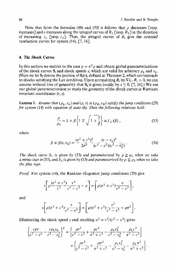
Note that from the formulas (49) and (50) it follows that p decreases [resp. increases] and/) increases along the integral curves of R1 [resp. R2] in the direction of increasing 21 [resp. •2]. Thus, the integral curves of Ri give the oriented rarefaction curves for system (14), [7, 16].
4. The Shock Curves
In this section we restrict to the case p = o'2p and obtain global parameterizations of the shock curves Si and shock speeds sl which are valid for arbitrary PL and VL. (Here we let Si denote the portion of Si(e), defined in Theorem 2, which corresponds to shocks satisfying the Lax condition. Upon normalizing Ri by V2i. Ri > 0, we can assume without loss of generality that Si is given locally by e < 0, [7, 16].) We use our global parameterization to study the geometry of the shock curves in Riemann invariant coordinates (r, s).
Lemma 1. Assume that (PL, VL) and (p, v) =- (PR,/)R) satisfy the jump conditions (29) for system (14) with equation of state (6). Then the following relations hold:
P = I + f l { I - T - / l + ~ } - - - - - - f ~ ( f l ) , p L (53)
where
(r + cZ)Z (v - vL) z fi ~ f l (v, VL) = 2 r z (c z _ v 2 ) ( c 2 _ v2 ) . (54 )
The shock curve $1 is given by (53) and parameterized by p > PL when we take a minus sign in (53), and $2 is given by (53) and parameterized by p < PL when we take the plus sign.
Proof For system (14), the Rankine-Hugoniot jump conditions (29) give
(o + c 2) v 2 S p C2 C 2 _ /)2
+ + 2 v
and
2 t) + /)2 + p 6 2 1
Eliminating the shock speed s and recalling U 2 = / ) 2 / ( C 2 - - / ) 2 ) gives
pv 2 pa 2 pLv~ pLz 2
• c2-v~ a~+c 2j
Global Solutions of the Relativistic Euler Equations 81
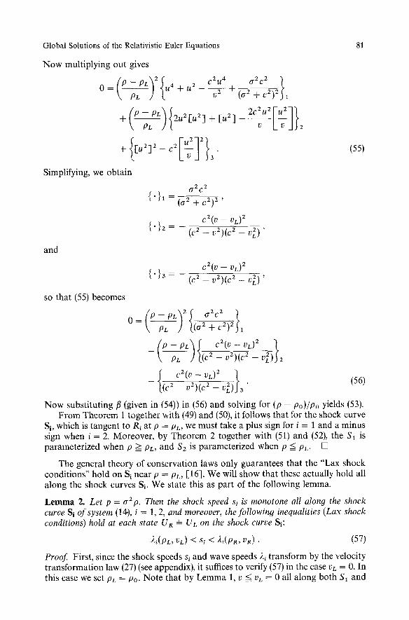
Now multiplying out gives
\ ~ ' ~ - L ] V [_ V _])2
+ ~ [ u = ] z - c 2 _ _ ( L V l J 3
J
Simplifying, we obtain
0-2C 2
�9 }1 -- (0.2 ...[_ C212 ,
c~(v _ v~) 2
�9 } ~ = - ( e ~ - v ~ ) ( c ~ - v ~ ) '
and
(55)
so that (55) becomes
c 2 ( v - v ~ t 2
�9 } ~ = - ( ~ - v ~ ) ( c ~ - v ~ ) '
_ _ c ~ ( v - v y
. f (c 2 c~(v _ v~) ~ ~_ ~ ~-c~ _--VL2)}3. (56t
Now substituting fl (given in (54)) in (56) and solving for (p - Po)/Po yields (53). From Theorem 1 together with (49) and (50), it follows that for the shock curve
Si, which is tangent to Ri at p = PL, we must take a plus sign for i = 1 and a minus sign when i = 2. Moreover, by Theorem 2 together with (51) and (52), the $1 is parameterized when p > PL, and $2 is parameterized when p < PL. []
The general theory of conservation laws only guarantees that the "Lax shock conditions" hold on SI near p = PL, [-16]. We will show that these actually hold all along the shock curves Si. We state this as part of the following lemma.
Lemma 2. Let p = 0-2p , Then the shock speed si is monotone all along the shock curve Si of system (14), i = 1, 2, and moreover, the following inequalities (Lax shock conditions) hold at each state UR �9 UL on the shock curve Si:
�9 ~i(PL, VL) < Sl < 2~(pR, VR)- (57)
Proof. First, since the shock speeds sl and wave speeds 2i transform by the velocity transformation law (27) (see appendix), it suffices to verify (57) in the case VL = 0. In this case we set PL = PO" Note that by Lemma 1, v < VL = 0 all along both SI and
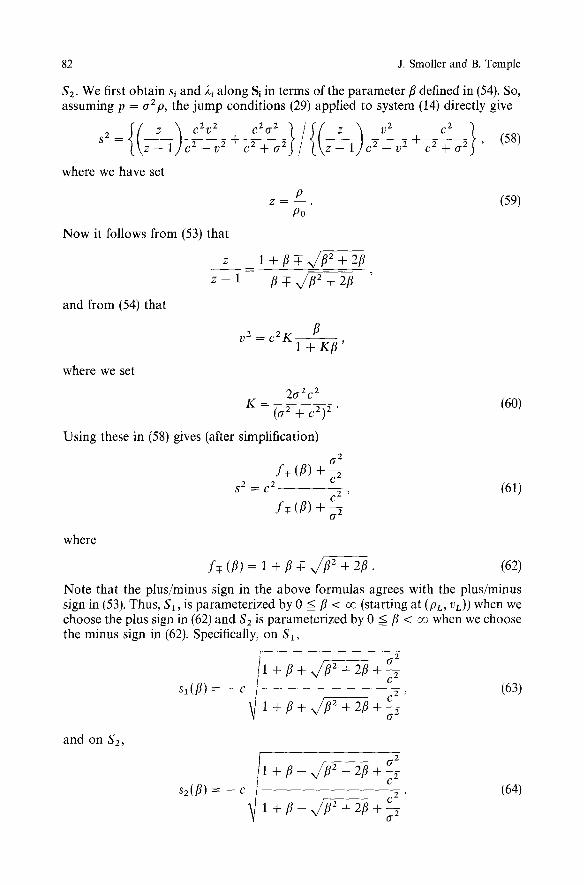
82 J. Smoller and B. Temple
$2. We first obtain si and 21 along Si in terms of the parameter fl defined in (54). So, assuming p = a2p, the jump conditions (29) applied to system (14) directly give
(\~7)U-x~-v" + c 2 + o-----~ ( \ z - i/c" - ~2 + c 2 + o-----~ , (ss)
where we have set
Now it follows from (53) that
2
Z - - 1
and from (54) that
where we set
P z = - - . (59) Po
1 + f l~ .,,/f12 + 2fl
fl-T- x/-~ + 2fl
V 2 = c 2 K fl 1 + I ( ~ '
262C 2 K - ((72 + c2)z . (60)
Using these in (58) gives (after simplification)
O-2 iT (fl) + ~-
S 2 = C 2 (61) r
f ~ (P) + 7~
where
f~_ (fl) = 1 + fi T- x/fl 2 + 2ft. (62)
Note that the plus/minus sign in the above formulas agrees with the plus/minus sign in (53). Thus, $1, is parameterized by 0 __< fi < ~ (starting at (PL, rE)) when we choose the plus sign in (62) and $2 is parameterized by 0 =< fi < ~ when we choose the minus sign in (62). Specifically, on Sa,
1 + fl + ~/fi2 + 2fl + ~-~ (63) s , ( f l ) = - c c2 ,
l + f l + ~ / + Z f l + ~
and on $2,
li o-' 1 + ~ - , f ~ + 2~ + ~ s~(/O = - c c . . (64)
Global Solutions of the Relativistic Euler Equations 83
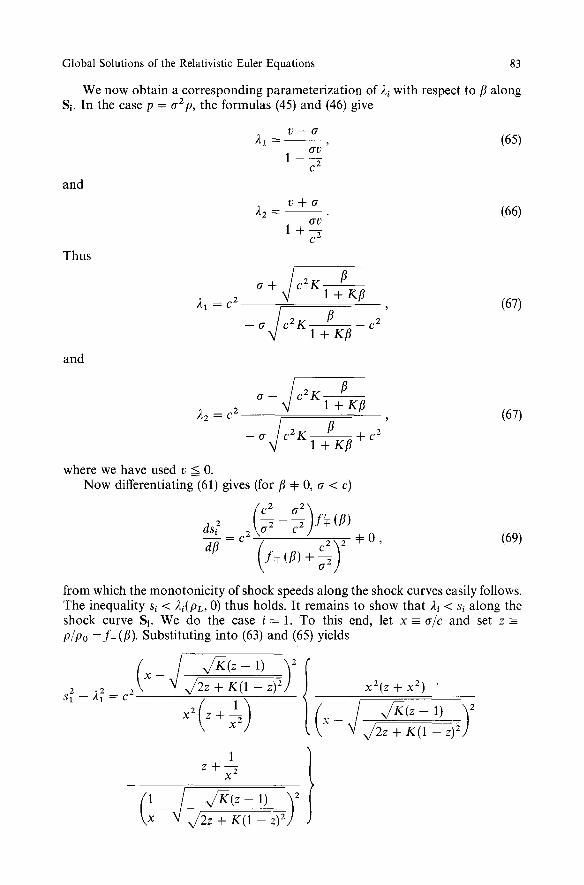
We now obtain a corresponding parameterization of 2~ with respect to fl along Si. In the case p = aZp, the formulas (45) and (46) give
and
Thus
V m 0 "
0"I) '
r
v + o - ~ " 2 - - - -
~TV 1+~
(65)
(66)
/ a + l c 2 K
21 = C 2 V 1 + Kfl , (67)
X/ ~ c 2 - a c Z K 1 + K f l
and
/ ff - - I c 2 K
•2 = C2 N/ 1 + Kfl , (67) l /~ r
-- a c2K 1 + K~ +
where we have used v < 0. Now differentiating (61) gives (for fl 4: 0, a < c)
ds~ c2 ~ f~ (fl) c 2"]2 4: 0 , (69)
dfl f r (fl) + t72 ]
from which the monotonicity of shock speeds along the shock curves easily follows. The inequality sl < 21(pL, 0) thus holds. It remains to show that 2~ < s~ along the shock curve Si. We do the case i = 1. To this end, let x =a/c and set z _= P/Po =f-(fl). Substituting into (63) and (65) yields
x2 ( 1 ) ( ~ x /K(z - - l) ) 2 K ( 1 -- z) 2 z + x - 1} Z + x z
(l_j
84 J. Smoller and B. Temple
- z , 2 , ,/2z + z)2 =c2 2{'},
where
{. }, = (xa(z + x2)) x/2z + K(1 - z) 2 - x//K(z - 1)
Thus it suffices to show that {. }. < 0. A calculation using the identities
x 4 + x 2 § 2 X 2 ~ K
and
leads to
x 2 + l 2
x - K '
(70)
23/2 } 2 _U,/2z K(1 z) 2 {. }, = (1 - x 2 ) ( 1 - ~) ~ + + - (71)
But by 2 (71) it follows that {.} < 0 for z > 1, and thus by (70) we must have sl - 21 < 0. Since both sl < 0 and 21 < 0 along $I when vL = 0, it follows that 21 < sl all along $1, thus finishing the proof of Lemma 2. [H
5. Geometry of the Shock Curves
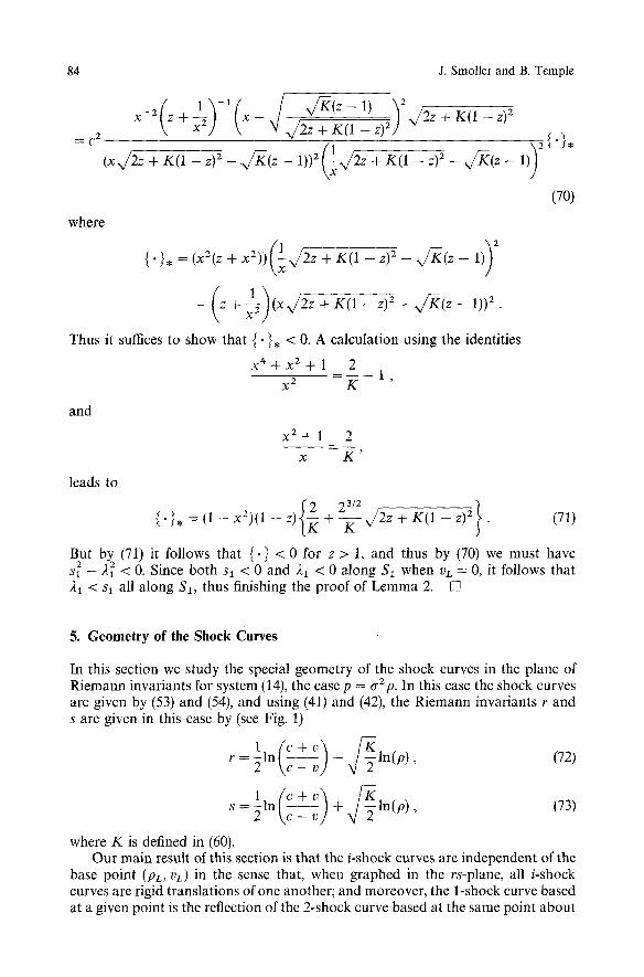
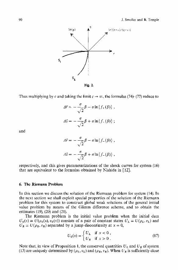
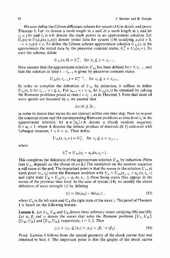
In this section we study the special geometry of the shock curves in the plane of Riemann invariants for system (14), the case p = aZp. In this case the shock curves are given by (53) and (54), and using (41) and (42), the Riemann invariants r and s are given in this case by (see Fig. 1)
r = 2 \ c - v ] - In(p), (72)
s = 2 \ c - v / + ln(p) , (73)
where K is defined in (60). Our main result of this section is that the/-shock curves are independent of the
base point (Pz, vr) in the sense that, when graphed in the rs-plane, all /-shock curves are rigid translations of one another; and moreover, the 1-shock curve based at a given point is the reflection of the 2-shock curve based at the same point about
Global Solutions of the Relativistic Euler Equations 85
In(p) ln((c+v)/(c-v)}
/ r-
Fig. 1.
an appropriate axis of rotation. On an algebraic level, this happens because, along
ashockcurve , p p [ l a n d ~ C + v ; ~ c + v z ~ -1 - - - - in the definitions of r and s turn out
(c - v ) ( c - vLJ to be functions of the parameter fl alone, and the functions that give pps ~ as a function of fl are reciprocal on the 1- and 2-shock curves, respectively. We begin with the following lemma, which gives a parameterization of the/-shock curves for system (14) in the rs-plane:
Lemma 3. Let r =- r(p, v), s - s(p, v), Ar =- r(p, v) - r(pL, vr) and As - s(p, v) - S(pL, VL), where we let (p, v) - (PR, VR). Then the 1-shock curve S1 for system (14) based at (rz, sz) is 9iven by the followin9 parameterization with respect to the parameter fl, 0 < fl < oo:
A r = - ~ l n { f + ( 2 K f l ) } - ~/~--~ln{f+(fl)} ,
As = -~ ln{f+(2Kf l )} + ~ f~ ln{f+( f l )} ;
and the 2-shock curve Sz based at (rz, SL) is 9iven for 0 <= fl < 0o, by
Ar = - ~ ln { f + (2Kfl) } - ~f~--ln{f_(fl)} ,
As= -~ln{f+(2Kfl)} + X/~ln{f_(f l )} .
(74)
(75)
(76)
(77)
Proof For convenience, define
C--V
C-t-V' (78)
so that
v 1 - - w
c l + w '
and by (72) and (73),
r + s = ln(w) .
86
Then by the definition of/7 in (54) we have
\ - c t , 7
+ w 1 + wL/ 4w 4wL
=7 - 4 w j ' which we can rewrite as
2 (Ar
J. Smoller and B. Temple
(79)
(80)
Now solving for w/wL in (79) gives
w 1 + 2Kfl 1 -T- + =--fr (2Kfl). (81) WL
Note that w is a monotone decreasing function of v, and v decreases along Si, i = 1, 2. Thus w/wt > 1 holds along Si, so that we must choose the plus sign in (81) on both/-shock curves. On the other hand, by (53), along the shock curves we have
P = f T (fl), (82) PL
where we take the plus sign when i = 1 and the minus sign when i = 2. Therefore, substituting (81) and (82) into (72) and (73), and choosing the appropriate plus and minus signs, gives (74)-(77). This completes the proof of Lemma 3. []
What is interesting about (74)-(77) is that the differences Ar and As along a shock curve depend only on the parameter/7, and thus the geometric shape of the shock curves in the rs-plane is independent of the base point (rz, sL). This immedi- ately implies that an /-shock curve based at one point in the rs-plane can be mapped by a rigid translation onto the/-shock curve based at any other point.
Lemma 4. The 2-shock curve based at an arbitrary point (rL, sL) is the reflection in the rs-plane of the 1-shock curve based at the same point, where the axis of reflection is the line passin9 through (rL, sL), parallel to the line r = s.
Proof This follows immediately from (74)-(77) because using (62) we have
The following lemma gives further important geometric properties of the shock curves which we shall need.
Global Solutions of the Relativistic Euler Equations 87
Lemma 5. The shock curves Si given in (74)-(77) define convex curves in the rs-plane, and moreover,
ds x / ~ - 1 0<dr r < _ x / ~ _ 1 < 1 (84)
all along a 1-shock curve Sa, and
dr x / 2 K - 1 < 1 (851 1 '
all along a 2-shock c u r v e S 2.
P r o o f By symmetry, it suffices to do the case i = 1. Differentiating (74) with respect to/3 gives
f d A r _ 1 1
d/3 x / ~ +/32 x/Z/3 + 2K/32'
and differentiating (75) with respect to/3 gives
so that
[ ~ dAs _ 1 1
4 K d - f l N / ~ -~/3 2 X/2/3 + 2K/3 2 '
dAs ds ~/2/3 + 2K/32 - ~ +/32 < 1 ,
dAr dr _ x/Z/3 + 2K/32 _ x/2/3 +/32
because 2K < 1. To verify the convexity of $1, we differentiate with respect to/3, and simplify to get
t -- ~2 q- 2K + + 1 + 2K + 1 > 0 . (86)
Now (84) follows from the convexity of the shock curves together with the inequality
lim ds x / ~ - 1 < 1 [] ~ dr - x / ~ - 1 -
A graph of the shock curves Si in the (r, s)-plane is given in Fig. 2. As a final comment in this section, we note that we can obtain a corresponding
parameterization of the shock curves for system (16) by taking the limit c -~ ~ . To see this, note that taking the limit c ~ ~ in (72) and (73) we obtain
? = cr --* v - o-In(p) , and
g - cs o v + rrln(p),
the right-hand sides being the Riemann invariants for system (16). Moreover, under this limit, (53) remains unchanged, and by (54),
(v - v ~ ) ~ 13 --* 28 z
88
Fig. 3,
J. Smoller and B. Temple
~v
U L ~ U~' Fig. 4.
U M ~ S I ( U L ) , and UReS2(U~t) then by (57),
s~ < ) t l ( U ~ ) < 2 ~ ( U u ) _-< s2 �9
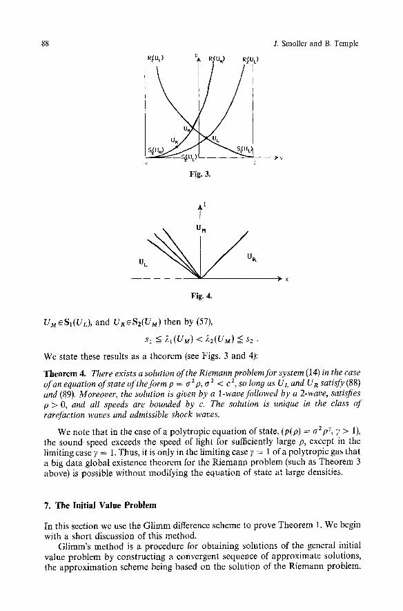
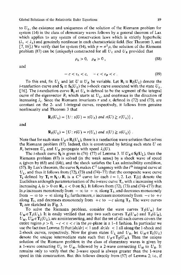
We state these results as a theorem (see Figs. 3 and 4):
Theorem 4. There exists a solution of the Riemann problem for system (14) in the case of an equation of state of the form p = (72 p , (72 < C 2, SO long as U L and U R satisfy (88) and (89). Moreover, the solution is 9iven by a 1-wave followed by a 2-wave, satisfies p > O, and all speeds are bounded by c. The solution is unique in the class of rarefaction waves and admissible shock waves.
We note that in the case of a polytropic equation of state, (p(p) = (72p~, 7 > 1), the sound speed exceeds the speed of light for sufficiently large p, except in the limiting case 7 = 1. Thus, it is only in the limiting case 7 = 1 of a polytropic gas that a big data global existence theorem for the Riemann problem (such as Theorem 3 above) is possible without modifying the equation of state at large densities.
7. The Initial Value Problem
In this section we use the Glimm difference scheme to prove Theorem 1. We begin with a short discussion of this method.
Glimm's method is a procedure for obtaining solutions of the general initial value problem by constructing a convergent sequence of approximate solutions, the approximation scheme being based on the solution of the Riemann problem.
Global Solutions of the Relativistic Euler Equations 89
to UL, the existence and uniqueness of the solution of the Riemann problem for system (t4) in the class of elementary waves follows by a general theorem of Lax which applies to any system of conservation laws which is strictly hyperbolic (21 </~2) and genuinely nonlinear in each characteristic field. (See Theorem 3, and [-7, 16].) We verify that for system (14), with p = 62/9, the solution of the Riemann problem (87) can be (uniquely) constructed for all UL and UR provided that
P L > 0 , O R > O , (88)
and
- c < v r < c , - - C < V R < C . (89)
TO this end, fix UL and let U - UR be variable. Let Ri -= Ri(Ur) denote the /-rarefaction curve and Si -= Si(UD the/-shock curve associated with the state Ur, [16]. The/-rarefaction curve Ri at Ur is defined to be the segment of the integral curve of the eigenvector R/which starts at Ur, and continues in the direction of increasing 2i. Since the Riemann invariants r and s, defined in (72) and (73), are constant on the 2- and 1-integral curves, respectively, it follows from genuine nonlinearity and Theorem 3 that
RI(Ur) = {U: s(U) = s(Ur) and r(U) > r(UL)} ,
and
R2(UL) = {U: r(U) = r(Ur) and s(U) >= s(UL)} .
Note that for each state UR ~ Ri(UL), there is a rarefaction wave solution that solves the Riemann problem (87). Indeed, this is constructed by letting each state U on Ri between UL and UR propagate with speed 2i(U).
The/-shock curve Si is given in (74)-(77) of Lemma 3. If UR ~ Si(UL), then the Riemann problem (87) is solved (in the weak sense) by a shock wave of speed s/(given by (63) and (64)), and the shock satisfies the Lax admissibility condition, (57). By Lax's theorem, the curve Si makes C 2 tangency with the ith integral curve at UL, and thus it follows from (72), (73) and (74)-77) that the composite wave curve T i defined by Ti - Si w Ri is a C 2 curve for each i = 1, 2. Let Ti(e) denote the Euclidean arclength parameterization of the/-wave curve Ti, with e increasing with increasing 2/(5 > 0 on Ri, e < 0 on Si). It follows from (72), (73) and (74)-(77) that In p increases monotonely from - oo to + oo along T1, and decreases monotonely from - oo to + oo along T~; furthermore, v increases monotonely from - c to + c along T1, and decreases monotonely from + c to - c along T2. The wave curves T i are sketched in Fig. 3.
To solve the Riemann problem, consider the wave curves T2(UM) for UMsTI(UL). It is easily verified that any two such curves T2(UM) and T2(U;t), UM, U~ e T1 (UL), are nonintersecting, and that the set of all such curves covers the entire region p > 0, - c < v < c in the pv-plane in a 1-1 fashion. In particular we use the fact (see Lemma 5) that Ids/drl < 1 and Idr/dsl < 1 all along the 1-shock and 2-shock curves, respectively. Now for given states UL and UR, let UM~TI(Ur) denote the unique intermediate state such that UReT2(UM). Then the unique solution of the Riemann problem in the class of elementary waves is given by a 1-wave connecting Ur to UM, followed by a 2-wave connecting UM to UR. It remains only to verify that the 2-wave speed is always greater than the 1-wave speed in this construction. But this follows directly from (57) of Lemma 2; i.e., if
90 J. Smoller and B. T emp le
S I
;n(p)
/ S z
Fig. 2.
In((c+v)/(C-V)}
/ r
Thus multiplying by c and taking the limit c ~ 0% the formulas (74)-(77) reduce to
o- A ~ - x/~/~ - o-ln{f+ (/~)} ,
and
A g = - - - (7
x / ~ / / + aln{f+(/?)} ;
o" A f - x/~/~ - a ln{ f_ (/~)} ,
respectively, and this gives parameterizations of the shock curves for system (16) that are equivalent to the formulas obtained by Nishida in [12].
6. The Riemann Problem
In this section we discuss the solution of the Riemann problem for system (14). In the next section we shall exploit special properties of the solution of the Riemann problem for this system to construct global weak solutions of the general initial value problem by means of the Glimm difference scheme, and to obtain the estimates (19), (20) and (21).
The Riemann problem is the initial value problem when the initial data Uo(x) - U(po(x) , Vo(X)) consists of a pair of constant states UL -- U(pL, VL) and UR -- U(pR, vR) separated by a jump discontinuity at x = 0,
UL if x < 0 , Uo(x) = UR if x > 0 . (87)
Note that, in view of Proposition 1, the conserved quantities UL and UR of system (13) are uniquely determined by (PL, VL) and (PR, vR). When UR is sufficiently close

Global Solutions of the Relativistic Euler Equations 91
The scheme consists of approximating the solution at a fixed time level by piecewise constant states, so that one can solve the resulting Riemann problems thereby obtaining a sequence of elementary waves at that time level, the goal being to estimate the growth in the amplitude of these elementary waves as the waves interact during the time evolution of the solution. Glimm's method provides a scheme by which Riemann problems are re-posed at a subsequent time level according to a random choice of the state appearing in the waves of the previous time level. This has the advantage that waves at the subsequent time level are determined through the interaction of waves at the prior time level, and by this scheme, estimates on the amplitude changes in waves during interactions can then be used to estimate the growth of a solution in general. The natural measure of the amplitude, or strength of a wave 7, is the magnitude of the jump I UR - ULI -= LTI. Thus, the total wave strength present in an approximate solution at time t > 0 is given by
t~il, (90) i
where the sum is over all waves present in the approximate solution at time t. The sum in (90) is equivalent to the total variation norm of the approximate solution at time t > 0. The total variation of the waves will in general increase due to interactions because of the nonlinearity of the equations. Glimm showed that for a strictly hyperbolic, genuinely nonlinear (or linearly degenerate [ 16]) system, if the total initial strength of waves in an approximate solution is sufficiently small (~ i I~1 ~ 1) at time t = 0, then the total strength of waves at time t > 0 is bounded by a constant times the initial strength. His method is to define a nonlocal functional Q, quadratic in wave strengths, which has the property that it decreases when waves interact, and moreover this decrease dominates the increase in total wave strength, when the initial wave strength is sufficiently small. This leads to the following theorem:
Theorem 5 (Glimm, [5]). Consider the initial value problem (23), (24)for a strictly hyperbolic, genuinely nonlinear system of conservation laws defined in a neighborhood of a state U . . Then there exist constants 0 < V ~ 1, C > O, and a neighborhood U of U. such that, if the initial data Uo lies in U, and
Var{U0(.)} < V, (91)
then there exists a global weak solution U(x, t) of (23), (24) obtained by Glimm's method, and this solution satisfies
Var{U(. , t)} < CVar{Uo(.)} . (92)
Glimm's method of analysis is the only method by which a time independent bound on wave strengths for a coupled nonlinear system of conservation laws has been rigorously proven. Glimm's method is also the only numerical method that has been proved to converge for the 3 x 3 classical Euler equations of gas dynamics. In this section we show that system (14) has the very special property that when p = cr2p, the total variation of ln(p) is nonincreasing (in time) when elementary waves interact. Thus, Var {ln(p)} plays the role of an energy function, and one can use this in place of the nonlocal functional Q in Glimm's method. This fact enables us to prove Theorem 1, a large data existence theorem, in this special case. (This idea is due to Nishida [12].)
92 J. Smoller and B. Temple
We now define the Gl imm difference scheme for system (14) in detail, and prove Theorem 1. Let Ax denote a mesh length in x and At a mesh length in t, and let xj = j A x and t, = nat denote the mesh points in an approximate solution. Let Uo(X) = U(po(x),vo(x)) denote initial data for system (14) satisfying po(X) > O, - c < Vo(X) < c. To define the Glimm scheme approximate solution U~x(x, t), we
approximate the initial data by the piecewise constant states, U ~ = Uo(xj+). To start the scheme, define
U ~ ( x , O ) = U ~ f o r x j < x < x j + l .
Now assume that the approximate solution UAx has been defined for t < t,_ 1, and that the solution at time t = t,_ i is given by piecewise constant states
n - U ~ x ( X , t , - 1 ) = U j 1, f o r x j < x < x j + l .
In order to complete the definition of U~x by induction, it suffices to define Ua~(x, t) for t._ 1 < t < t,. For t,_ ~ < t < t,, let Uax(x, t) be obtained by solving the Riemann problems posed at time t = t,_ 1 as in Theorem 3. Note that since all wave speeds are bounded by c, we assume that
Ax/At > 2c,
in order to insure that waves do not interact within one time step. Now to re-pose the constant states and the corresponding Riemann problems at time level t, in the approximate solution, let a - - -{ak}~A denote a (fixed) random sequence, 0 < ak < 1, where A denotes the infinite product of intervals (0, 1) endowed with Lebesgue measure, 1 < k < or. Then define
U~(x , t ,+) = U~., for xj < x < xj+l ,
where
U] = UAx(Xj + andX, t , - ) .
This completes the definition of the approximate solution UAx by induction. (Note that Uax depends on the choice of a ~ A.) The restriction on the random sequence a will come at the end. The important point is that the waves in the solution Uax at mesh point (xj, t,) solve the Riemann problem with UL = Udx(xj-1 -~ a, Ax, tn-- ) and right state UR = UAx(Xj + a, Ax, t,--), these being states that appear in the waves of the previous time level. In the case of system (14), we modify the above definition of wave strength 17[ by defining
171 = Iln(pR) - ln(pL)[, (93)
where Uz is the left state and UR the right state of the wave 7. The proof of Theorem 1 is based on the following lemma:
Lemma 6. Let UL, U M and UR denote three arbitrary states satisfying (88) and (89). Let ~i, fli and 7i denote the waves that solve the Riemann problems [UL, UM], [Uu , UR] and [UL, UR], respectively, i = 1, 2. Then
171[ + 1721 < lel] + lezl + Ifll[ + ]fief. (94)
Proof. Lemma 6 follows from the special geometry of the shock curves that was obtained in Sect. 5. The important point is that the graphs of the shock curves
Global Solutions of the Relativistic Euler Equations 93
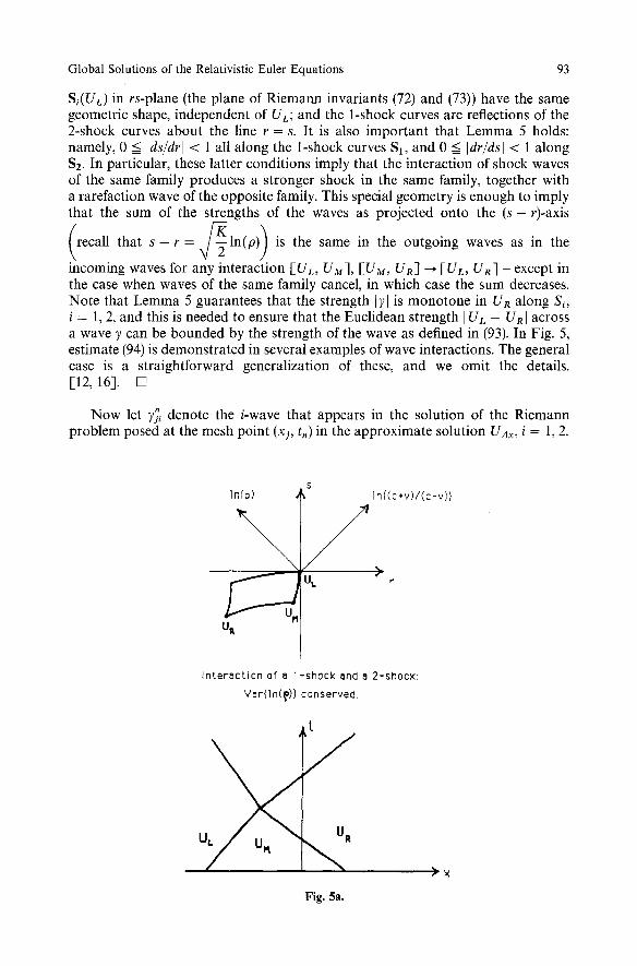
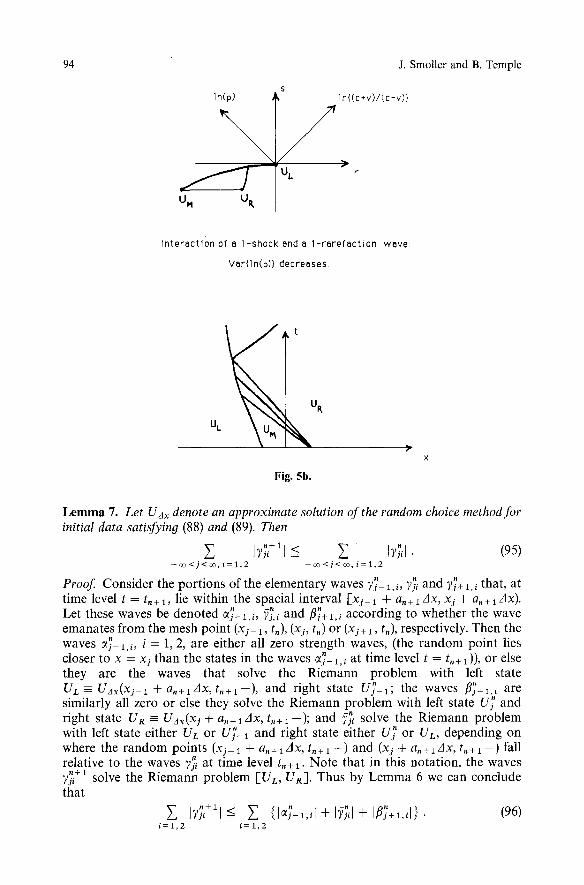
SI(UL) in rs-plane (the plane of Riemann invariants (72) and (73)) have the same geometric shape, independent of UL; and the 1-shock curves are reflections of the 2-shock curves about the line r = s. It is also important that Lemma 5 holds: namely, 0 < I ds/drl < 1 all along the 1-shock curves St, and 0 < I dr/dsl < 1 along $2. In particular, these latter conditions imply that the interaction of shock waves of the same family produces a stronger shock in the same family, together with a rarefaction wave of the opposite family. This special geometry is enough to imply that the sum of the strengths of the waves as projected onto the ( s - 0-axis /
(recall that s - r = \ / ~ l n ( p ) ) i s the same in the outgoing waves as in the k
incoming waves for any interaction [UL, UM], [UM, UR] --* [UL, UR] - except in the case when waves of the same family cancel, in which case the sum decreases. Note that Lemma 5 guarantees that the strength fT] is monotone in UR along Si, i = 1, 2, and this is needed to ensure that the Euclidean strength I UL -- URI across a wave 7 can be bounded by the strength of the wave as defined in (93). In Fig. 5, estimate (94) is demonstrated in several examples of wave interactions. The general case is a straightforward generalization of these, and we omit the details. [12, 16]. []
Now let 7j"~ denote the /-wave that appears in the solution of the Riemann problem posed at the mesh point (xj, t,) in the approximate solution UAx, i = 1, 2.
ln(p)
U~
S ]n{ (c*v) / (c-v)}
S >
U i . r
Interact ion of a 1-shock and a 2-shock:
Vor(ln(l~)} conserved.
.q, Fig. 5a.
) x
94 J. Smoller and B. Temple
In(p)
U M Up,
ln{(c+v)/(c-v))
/
Interaction of a l-shock anda l-rarefaction wave:
Var{In(9)} decreases.
t
K
U c
Fig. 5b.
•
L e m m a 7. Let U ~x denote an approximate solution of the random choice method for initial data satisfying (88) and (89). Then
177i+ 1 " . E J" 1< E IVii] �9 (95) - - m < j < o o , i = l , 2 - o o < j < oe, i= 1 ,2
n n n Proof. Consider the por t ions of the e lementary waves 7i-1. i, Vj'i and 7j+ t, ~ that, at t ime level t = t .+ l , lie within the spacial interval [ x j - t + a.+~Ax, xj + a.+lAX).
n -n n Let these waves be denoted %_~,~, 7j, i and flj+l,i according to whether the wave emanates f rom the mesh point (xj_ 1, t.), (x j, t.) or (x j+ l, t.), respectively. Then the waves c~.-1,i, i = 1, 2, are either all zero strength waves, (the r andom point lies
n closer to x = xj than the states in the waves cg_a,~ at t ime level t = t .+l)) , or else they are the waves that solve the Riemann p rob lem with left state UL--UAx(Xj-z + a.+lAX, t.+l--), and right state U~_~; the waves fl~+l,~ are similarly all zero or else they solve the Riemann p rob lem with left state U~ and right state U R - Udx(xj + a.+tAx, 6+1- - ) ; and ~.; solve the Riemann prob lem with left state either UL or Uy- t and right state either Uy or UL, depending on where the r a n d o m points (xj-1 + a.+ ~ Ax, t . + l - ) and (xj + a.+ l Ax, t.+ l - ) fall relative to the waves 7j'," at t ime level t.+ ~. Note that in this notat ion, the waves ?,".~+ ~ solve the Riemann prob lem [UL, UR]. Thus by L e m m a 6 we can conclude J that
Z n + t -n n ?ji I X Z { l ~ ; - 1 , 1 l "~ I~jl[-]" Iflj+l,il}" ( 9 6 ) i = 1 , 2 i = 1 , 2

Global Solutions of the Relativistic Euler Equations 95
But summing j from -- ~ to + ~ in (96) and rearranging terms gives n n n
Z j : ~ , i , j i , j i , j
the latter inequality holding because, by construction, - n I%"~I + [~j~l + I/~}I = I~}[.
This completes the proof of Lemma 6. []
We now complete the proof of Theorem 1. First, since ln(p) is monotone along the wave curves Ti, it follows that at time level te( t , , t ,+l) in an approximate solution UAx, the sum of the strengths of the waves at time t is equivalent to the total variation in ln(p) of the approximate solution at time t:
Var{ln(p~x(-, t))} = ~ [Tj"~[ �9 (97) i , j
Thus, in the approximate solution,
Var{ln(p~x(., t+))} < Var{ln(p~x(., s + ) ) } , (98)
whenever s < t. We now note that by Helly's theorem [16], L 1 limits of functions of uniformly bounded variation satisfy the same variation bound. This gives the first inequality (19) of Theorem 1 for any weak solution U(x, t) = U(p(x, t), v(x, t)) obtained as an L 1 limit of approximate solutions UAx as Ax ~ O. Thus we show that (19) of Theorem 1 is a consequence of the following lemma:
Lemma 8 (Glimm, [5]). Assume that the approximate solution U ~x satisfies
Var{UA~(., t)} < V < ~ (99)
for all t > O. Then there exists a subsequence of mesh lengths Ax ~ 0 such that U~x ~ U, where U(x, t) also satisfies (99). The approximate solutions converge pointwise a.e., and in L~o~ at each time, uniformly on bounded x and t sets. Moreover, there exists a set N c A of Lebesgue measure zero such that, if a e A - N, then U(x, t) is a weak solution of the initial value problem (14), (15).
Using Lemma 8, the proof of (19) and (20) of Theorem 1 is completed once we show that the estimates (17) and (18) imply (99) for the approximate Glimm scheme solutions. For this, note that (17) and (18) imply that there exist states P~o = l i m x ~ po(x) and u~ = l i m x ~ Uo(X). But (18) implies that the total variation
in In ~ ) is finite at time t -- 0+ in the approximate solution UA~, and thus
Var{ln(pAx(-, 0+))} < Vo ,
where Vo depends only on the initial total variation bounds in (17) and (18). Thus, by (98),
Var{ln(pAx(-, t+))} < Vo, (100)
for all positive times t > 0. But it follows directly from (85) and (84) of Lemma 5
that the variation in In e-~--~_ v j _ _ is bounded uniformly by the variation in ln(p)
across every elementary wave in each approximate solution UA~. Thus (100)
96
implies that
J. Smoller and B. Temple
at each t > 0 in an approximate solution U~x, where V~ depends only on Vo. It now follows from (100) and (101) that for every A x and a ~ A, p~ = limx-~| PAx(X, t) and v~ = limx-~o VAx(X, t). This means that (p~, v~) is a constant state appearing in the approximate solutions at each fixed time level. This together with (100) and (10l) implies that there exists a constant M > 0 such that
1 / M < PAx(X, t) < M ,
and
- c + 1 / M < VAx(X, t) < C-- 1 / M ,
for all x and t > 0, uniformly in Ax. The desired result (99) follows from these latter two bounds because, in light of Proposition 1, the Jacobian determinant
~(U1, U2) I ~(p, v) is bounded away from zero (uniformly in Ax) on the image of the
approximate solutions UAx. Thus by Lemma 8 there exists a subsequence of mesh lengths A x ~ 0 such that U Ax ~ U(p(x , t), v(x, t)) where U satisfies (99), (19) and (20), and the convergence is pointwise a.e., and in Llloc at each time, uniformly on bounded x and t sets. By Proposition 2, Vo and V~ must be Lorentz invariant constants.
8. Appendix I
In this section we show that the transformation properties of characteristics and shocks in a relativistic system of conservation laws follows directly from the covariance properties of the Rankine-Hugoniot jump relations alone. In particu- lar, we show that the characteristic curves and shock curves associated with a system of conservation laws div T = 0, transform, under general nonlinear spacetime coordinate transformations, like the level curve of a scalar function. We assume that the divergence is taken with respect to a Lorentz metric g defined in four dimensional spacetime. As a consequence, we show that the wave speeds 2~ and the shock speeds sl, defined for systems (9) and (14), transform according to the special relativistic velocity transformation law (12).
Thus, if gii denotes a fixed Lorentzian metric defined on a four dimensional spacetime x = (x ~ . . . . . x3), x ~ = ct, let F)k denote the Christoffel symbols which define the unique symmetric connection associated with glj, namely
F jik _= 1 i~ ~ g ~g.j,k + gk., j -- gik,~} �9
Let T~) be a symmetric (0, 2)-tensor which we take to be the stress energy tensor for some field in spacetime. Conservation of energy-momentum based on the metric g then reads div T = 0, where the covariant divergence is given in coordinates by [20, 43
div T =- T "~ T "~ ~ ~ -- FjaT~ a . j; ~ j, ~ + F~ Tj (102)
Here, ", i" denotes Q/Ox ~ and "; i" denotes the covariant derivative.
Global Solutions of the Relativistic Euler Equations 97
Definition 1. Assume that T~j (defined in a given coordinate system x) is smooth except for a jump discontinuity across a smooth surface q$(x) = 0, where dga - n~dx ~ :k O. Then we say that T is a weak solution ofdiv T = 0 if this equation holds away from the surface ~b(x)= 0, and across the surface the following (Rankine-Hugoniot) jump conditions hold:
[T~n~] = O. (103)
Here, as usual, the square brackets around a quantity denote the jump in the quantity across the surface 4b = 0,
=- ( T ; n . ) , , - (T;n )L = [ T ; ] n o .
One can show that the jump relation is implied by the weak formulation of div T = 0 in the sense of the theory of distributions [16], and implies conservation of the physical energy-momentum across the surface of discontinuity q$ = 0. The equivalence of the weak formulation follows from integration by parts, observing that the non-divergence terms F~ T] - Fj~ T~ contain no derivative of T.
From the jump conditions we obtain the following proposition:
Proposition A1. A shock surface transforms (under arbitrary nonlinear changes of spacetime coordinates)' as the level curve of a scalar function defined on spacetime.
Proof. If ITS] ni = 0 holds on the surface ~b = 0 in one coordinate system x where d(J = ni dx ~, then it holds in every other coordinate system because T transforms like a (1, 1)-tensor, and dq$ is a 1-form. []
Now restricting to a 2-dimensional Minkowski spacetime, so that gig = rhj, Proposition A1 implies that the shock curve has tangent vector dx/dz = X if and only ifn~dxi(X) = 0, where nidx i = dc~ and ~b is a function constant along the shock curve. Thus, letting X ~ denote the components of X, we conclude that the shock speed s = dxl/dt is given by
X 1 no S -~- C - ~ ~ - - C - - .
n l
Proposition A2. Under Lorentz transformations, the shock speeds s transform ac- cording to the velocity transformation rule (12).
Proof. Consider a Lorentz transformation taking the unbarred coordinates x i to the barred coordinates if', such that the barred frame moves with velocity/x as measured in the unbarred frame x( Then
= A ( u ) T x ' ,
Fcosh(0) sinh(0)
A(/0~ = [_sinh(0) cosh(0)_J'
where
(106)
and tanh(0) = ~t/c, [20]. Then the vector X, tangent to the shock curve, transforms a s
2 = = A(ix)~X i .

98 J. Smoller and B. Temple
Thus in the ba r red coordinates , the shock speed is given by
)~1 X ~ cosh(0) + X 1 sinh(0) /~ + s
s= C-x 6 = Cx~ + X1 cosh(0) = /~v 1 +
J
This completes the p roo f of P ropos i t i on A2. []
Proposition A3. The characteristic curves for a system of conservation laws (23) transform as level curves of functions in physical space. Moreover, under Lorentz transformations, the wave speeds 2~ (the eigenvalues of dF) transform according to the velocity transformation law (12).
Proof By Theorem 2, /~i = l i m ~ o si(e). Thus, by cont inui ty, 21 t ransforms as a veloci ty (12) under Loren tz t r ans format ions because s~(e) does for each fixed e. Since the character is t ic curves are given by dxl/dt = 2~ and 2i t ransforms as a velocity, it follows tha t the character is t ic curves mus t t ransform like level curves of functions. Thus by duali ty, in two d imens iona l spacet ime, the tangents to the shock curves and character is t ic curves t ransform like vectors. []
References
1. Anile, A.M.: Relativistic Fluids and Magneto-Fluids. Cambridge Monographs on Mathemat- ical Physics, Cambridge: Cambridge University Press 1989
2. Christodoulou, D.: Private communication 3. Courant, R., Friedrichs, K.O.: Supersonic Flow and Shock Waves. New York: Wiley 1948 4. Dubrovin, B.A., Fomenko, A.T., Novikov, S.P.: Modern Geometry-Methods and Applica-
tions. Berlin, Heidelberg, New York: Springer 1984 5. Glimm, J.: Solutions in the large for nonlinear hyperbolic systems of equations. Commun,
Pure Appl. Math. 18, 697-715 (1965) 6. Johnson, M., McKee, C. : Relativistic hydrodynamics in one dimension. Phys. Rev. D, 3, no. 4,
858-863 (197l) 7. Lax, P.D.: Hyperbolic systems of conservation laws, II. Commun. Pure Appl. Math. 10,
537 566 (1957) 8. Liu, T.P.: Private communication 9. Luskin, M., Temple, B.: The existence of a global weak solution of the waterhammer problem.
Commun. Pure Appl. Math. 35, 697-735 (1982) 10. McVittie, G.C.: Gravitational collapse to a small volume. Astro. Phys. J. 140, 401 416 (1964) 11. Misner, C., Sharp, D.: Relativistic equations for adiabatic, spherically symmetric gravi-
tational collapse. Phys. Rev. 26, 571-576 (1964) 12. Nishida, T.: Global solution for an initial boundary value problem ofa quasilinear hyperbolic
system. Proc. Jap. Acad. 44, 642-646 (1968) 13. Nishida, T., Smoller, J.: Solutions in the large for some nonlinear hyperbolic conservation
laws. Commun. Pure Appl. Math. 26, 183-200 (1973) 14. Oppenheimer, J.R., Snyder, J.R.: On continued gravitational contraction. Phys. Rev. 56,
455-459 (1939) 15. Oppenheimer, J.R., Volkoff, G.M.: On massive neutron cores. Phys. Rev. tiff, 374-381 (1939) 16. Smoller, J.: Shock Waves and Reaction Diffusion Equations. Berlin, Heidelberg, New York:
Springer 1983 17. Taub, A.: Approximate solutions of the Einstein equations for isentropic motions of plane-
symmetric distributions of perfect fluids. Phys. Rev. 107, no. 3, 884-900 (1957)

Global Solutions of the Relativistic Euler Equations 99
18. Thompson, K.: The special relativistic shock tube. J. Fluid Mech. 171, 365 375 (1986) 19. Tolman, R.: Relativity, Thermodynamics and Cosmology. Oxford: Oxford University Press
1934 20. Weinberg, S.: Gravitation and Cosmology: Principles and Applications of the General
Theory of Relativity. New York: Wiley 1972
Communicated by S.-T. Yau