In Defense of Classical Image Processing: Fast Depth Completion on the CPU

Jason Ku, Ali Harakeh, and Steven L. Waslander

Mechanical and Mechatronics Engineering DepartmentUniversity Of WaterlooWaterloo, ON, Canada

jason.ku@uwaterloo.ca, www.aharakeh.com, stevenw@uwaterloo.ca

Abstract—With the rise of data driven deep neural networksas a realization of universal function approximators, mostresearch on computer vision problems has moved away fromhand crafted classical image processing algorithms. This papershows that with a well designed algorithm, we are capable ofoutperforming neural network based methods on the task ofdepth completion. The proposed algorithm is simple and fast,runs on the CPU, and relies only on basic image processingoperations to perform depth completion of sparse LIDARdepth data. We evaluate our algorithm on the challengingKITTI depth completion benchmark [1], and at the time ofsubmission, our method ranks first on the KITTI test serveramong all published methods. Furthermore, our algorithm isdata independent, requiring no training data to perform thetask at hand. The code written in Python will be made publiclyavailable at https://github.com/kujason/ip basic.

Keywords-image processing; depth completion.

I. INTRODUCTION

The realization of universal function approximators viadeep neural networks has revolutionized computer vision andimage processing. Deep neural networks have been used toapproximate difficult high dimensional functions involved inobject detection [2], semantic and instance level segmenta-tion [3], and even the decision making process for drivinga car [4]. The success of these function approximators onAI-complete [5] tasks has lead the research community tostray away from classical non-learning based methods tosolve almost all problems. This paper aims to show thatwell-designed classical image processing algorithms can stillprovide very competitive results compared to deep learningbased methods. We specifically tackle the problem of depthcompletion, that is, inferring a dense depth map from imageand sparse depth map inputs.

Depth completion is an important task for machine visionand robotics. Current state-of-the-art LIDAR sensors canonly provide sparse depth maps when projected back toimage space. This limits both the performance and theoperational range of many perception algorithms that relyon the depth as input. For example, 3D object detectionalgorithms [2], [6], [7] can regress bounding boxes only ifthere are enough points belonging to the object.

Many different approaches have been proposed for depthcompletion. These approaches range from simple bilateralupsampling based algorithms [8] to end-to-end deep learningbased ones [9]. The latter are very attractive as they requireminimal human design decisions due to their data drivennature. However, using deep learning approaches results inmultiple consequences. First, there is finite compute poweron embedded systems. GPUs are very power hungry, anddeploying a GPU for each module to run is prohibitive.Second, the creation of deep learning models without properunderstanding of the problem can lead to sub-optimal net-work designs. In fact, we believe that solving this problemwith high capacity models can only provide good resultsafter developing sufficient understanding of its underlyingintricacies through trying to solve it with classical imageprocessing methods.

This paper aims to show that on certain problems, deeplearning based approaches can still be outperformed bywell designed classical image processing based algorithms.To validate this, we design a simple algorithm for depthcompletion that relies on image processing operations only.The algorithm is non-guided and relies on LIDAR data only,making it independent of changes in image quality. Further-more, our algorithm is not deep learning based, requiringno training data, making it robust against overfitting. Thealgorithm runs as fast as deep learning based approachesbut on the CPU, while performing better than the customdesigned sparsity invariant convolutional neural network of[9]. To summarize, our contributions are as follows:

• We provide a fast depth completion algorithm that runsat 90 Hz on the CPU and ranks first among all publishedmethods on the KITTI depth completion benchmark[10].

• We show that our algorithm outperforms CNN basedapproaches that have been designed to tackle sparseinput representations by a wide margin.

The rest of this paper is structured as follows: SectionII provides a brief overview of state-of-the-art depth com-pletion algorithms. Section IV describes the problem ofdepth completion from a mathematical perspective and then

arX

iv:1

802.

0003

6v1

[cs

.CV

] 3

1 Ja

n 20

18

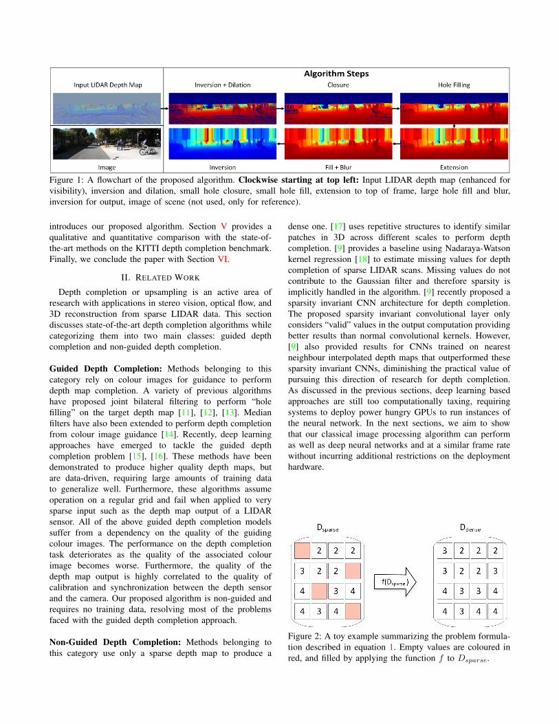
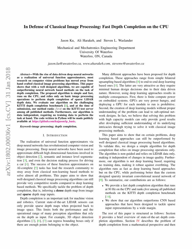
Figure 1: A flowchart of the proposed algorithm. Clockwise starting at top left: Input LIDAR depth map (enhanced forvisibility), inversion and dilation, small hole closure, small hole fill, extension to top of frame, large hole fill and blur,inversion for output, image of scene (not used, only for reference).

introduces our proposed algorithm. Section V provides aqualitative and quantitative comparison with the state-of-the-art methods on the KITTI depth completion benchmark.Finally, we conclude the paper with Section VI.

II. RELATED WORK

Depth completion or upsampling is an active area ofresearch with applications in stereo vision, optical flow, and3D reconstruction from sparse LIDAR data. This sectiondiscusses state-of-the-art depth completion algorithms whilecategorizing them into two main classes: guided depthcompletion and non-guided depth completion.

Guided Depth Completion: Methods belonging to thiscategory rely on colour images for guidance to performdepth map completion. A variety of previous algorithmshave proposed joint bilateral filtering to perform “holefilling” on the target depth map [11], [12], [13]. Medianfilters have also been extended to perform depth completionfrom colour image guidance [14]. Recently, deep learningapproaches have emerged to tackle the guided depthcompletion problem [15], [16]. These methods have beendemonstrated to produce higher quality depth maps, butare data-driven, requiring large amounts of training datato generalize well. Furthermore, these algorithms assumeoperation on a regular grid and fail when applied to verysparse input such as the depth map output of a LIDARsensor. All of the above guided depth completion modelssuffer from a dependency on the quality of the guidingcolour images. The performance on the depth completiontask deteriorates as the quality of the associated colourimage becomes worse. Furthermore, the quality of thedepth map output is highly correlated to the quality ofcalibration and synchronization between the depth sensorand the camera. Our proposed algorithm is non-guided andrequires no training data, resolving most of the problemsfaced with the guided depth completion approach.

Non-Guided Depth Completion: Methods belonging tothis category use only a sparse depth map to produce a

dense one. [17] uses repetitive structures to identify similarpatches in 3D across different scales to perform depthcompletion. [9] provides a baseline using Nadaraya-Watsonkernel regression [18] to estimate missing values for depthcompletion of sparse LIDAR scans. Missing values do notcontribute to the Gaussian filter and therefore sparsity isimplicitly handled in the algorithm. [9] recently proposed asparsity invariant CNN architecture for depth completion.The proposed sparsity invariant convolutional layer onlyconsiders “valid” values in the output computation providingbetter results than normal convolutional kernels. However,[9] also provided results for CNNs trained on nearestneighbour interpolated depth maps that outperformed thesesparsity invariant CNNs, diminishing the practical value ofpursuing this direction of research for depth completion.As discussed in the previous sections, deep learning basedapproaches are still too computationally taxing, requiringsystems to deploy power hungry GPUs to run instances ofthe neural network. In the next sections, we aim to showthat our classical image processing algorithm can performas well as deep neural networks and at a similar frame ratewithout incurring additional restrictions on the deploymenthardware.

Figure 2: A toy example summarizing the problem formula-tion described in equation 1. Empty values are coloured inred, and filled by applying the function f to Dsparse.

Figure 3: Different kernels used for comparison.

III. PROBLEM FORMULATION

The problem of depth completion can be described asfollows:Given an image I ∈ RM×N , and a sparse depth mapDsparse ∈ RM×N find f that approximates a true functionf : RM×N × RM×N → RM×N where f(I,Dsparse) =Ddense. The problem can be formulated as:

min. ||f(I,Dsparse)− f(I,Dsparse)||2F = 0 (1)

Here, Ddense is the output dense depth map, and has thesame size as I and Dsparse with empty values replacedby their depth estimate. In the case of non-guided depthcompletion, the above formulation becomes independent ofthe image I as shown in Fig. 2. We realize f via a seriesof image processing operations described below.

IV. PROPOSED ALGORITHM

The proposed method, as shown in Fig. 1 is implementedin Python and uses a series of OpenCV [19] and NumPy[20] operations to perform depth completion. We leveragethe implementation of standard OpenCV operations, whichuse larger pixel values to overwrite lower pixel values. Thisway, the issue of sparsity can be addressed by selecting ap-propriate operations to fill in empty pixels. By exploiting thisproperty of OpenCV operations, we realize depth completionvia the eight step algorithm described below.

The final result of the algorithm is a dense depth mapDdense that can be used as input for 3D object detection,occupancy grid generation, and even simultaneous localiza-tion and mapping (SLAM).

1) Depth Inversion: The main sparsity handling mecha-nisms employed are OpenCV morphological transformationoperations, which overwrite smaller pixel values with largerones. When considering the raw KITTI depth map data,

closer pixels take values close to 0 m while further onestake values up to a maximum of 80 m. However, emptypixels take the value 0 m too, which prevents using nativeOpenCV operations without modification. Applying a dila-tion operation on the original depth map would result inlarger distances overwriting smaller distances, resulting inthe loss of edge information for closer objects. To resolvethis problem, valid (non-empty) pixel depths are invertedaccording to Dinverted = 100.0−Dinput, which also createsa 20 m buffer between valid and empty pixel values. Thisinversion allows the algorithm to preserve closer edges whenapplying dilation operations. The 20 m buffer is used tooffset the valid depths in order to allow the masking ofinvalid pixels during subsequent operations.

2) Custom Kernel Dilation: We start by filling emptypixels nearest to valid pixels, as these are most likely to shareclose depth values with valid depths. Considering both thesparsity of projected points and the structure of the LIDARscan lines, we design a custom kernel for an initial dilationof each valid depth pixel. The kernel shape is designed suchthat the most likely pixels with the same values are dilatedto the same value. We implement and evaluate four kernelshapes shown in Fig. 3. From the results of the experimentsperformed in Section V, a 5× 5 diamond kernel is used todilate all valid pixels.

3) Small Hole Closure: After the initial dilation step,many holes still exist in the depth map. Since these areascontain no depth values, we consider the structure of objectsin the environment and note that nearby patches of dilateddepths can be connected to form the edges of objects. Amorphological close operation, with a 5 × 5 full kernel, isused to close small holes in the depth map. This operationuses a binary kernel, which preserves object edges. This stepacts to connect nearby depth values, and can be seen as aset of 5× 5 pixel planes stacked from farthest to nearest.

4) Small Hole Fill: Some small to medium sized holesin the depth map are not filled by the first two dilationoperations. To fill these holes, a mask of empty pixels isfirst calculated, followed by a 7 × 7 full kernel dilationoperation. This operation results in only the empty pixelsbeing filled, while keeping valid pixels that have beenpreviously computed unchanged.

5) Extension to Top of Frame: To account for tall objectssuch as trees, poles, and buildings that extend above thetop of LIDAR points, the top value along each column isextrapolated to the top of the image, providing a denserdepth map output.

6) Large Hole Fill: The final fill step takes care of largerholes in the depth map that are not fully filled from previoussteps. Since these areas contain no points, and no image datais used, the depth values for these pixels are extrapolatedfrom nearby values. A dilation operation with a 31x31 fullkernel is used to fill in any remaining empty pixels, whileleaving valid pixels unchanged.

Sparse CNN Nearest Neighbor Interpolation + CNN Ours

Figure 4: The qualitative results of our proposed algorithm on three samples in the KITTI test set in comparison to SparseCNN and Nearest Neighbour Interpolation with CNN, both of which were proposed in [9]. Top: Output dense depth map.Bottom: Visualization of the pixel-wise error in estimation ranging from blue for a low error to red for a high error. It canbe seen that our method has a lower error in estimation especially for further away pixels.

7) Median and Gaussian Blur: After applying the pre-vious steps, we end up with a dense depth map. However,outliers exist in this depth map as a by-product of the dilationoperations. To remove these outliers, we use a 5× 5 kernelmedian blur. This denoising step is very important as itremoves outliers while maintaining local edges. Finally, a5×5 Gaussian blur is applied in order to smooth local planesand round off sharp object edges.

8) Depth Inversion: The final step of our algorithm is torevert back to the original depth encoding from the inverteddepth values used by the previous steps of the algorithm.This is simply calculated as Doutput = 100.0−Dinverted.

V. EXPERIMENTS AND RESULTS

We test our algorithm’s performance on the depth com-pletion task in the KITTI depth completion benchmark. Therecently released depth completion benchmark contains alarge set of LIDAR scans projected into image coordinatesto form depth maps. The LIDAR points are projected tothe image coordinates using the front camera calibrationmatrices, resulting in a sparse depth map with the samesize as the RGB image. The sparsity is induced by thefact that LIDAR data has a much lower resolution thanthe image space it is being projected to. Due to the anglesof LIDAR scan lines, only the bottom two-thirds of thedepth map contain points. The sparsity of the points in thebottom region of the depth maps is found to range between5 − 7%. The corresponding RGB image is also provided

for each depth map, but is not used by our unguided depthcompletion algorithm. The provided validation set of 1000images is used for evaluation for all experiments, and thefinal results on the 1000 image test set are submitted andevaluated by KITTI’s test server. The performance of thealgorithm and the baselines are evaluated using the inverseRoot Mean Squared Error (iRMSE), inverse Mean AverageError (iMAE), Root Mean Squared Error (RMSE), and MeanAverage Error (MAE) metrics. We refer the reader to [9] fora deeper insight on each of these metrics. Since methods areranked based on RMSE on KITTI’s test server, the RMSEmetric is used as the criterion for selecting the best design.

A. Performance on the Depth Completion Task

At the time of submission, the proposed algorithm ranksfirst among all published methods in both RMSE and MAEmetrics. Table I provides the results of comparison againstthe baseline Nadaraya-Watson kernel method (NadarayaW),as well as the learning based approaches Sparsity InvariantCNNs (SparseConvs) and Nearest Neighbour Interpolationwith CNN (NN+CNN) [9], all of which are specificallytailored for processing sparse input. Our algorithm outper-forms the NN+CNN, the runner up on the KITTI data set,by 131.29 mm in RMSE and 113.54 mm in MAE. That isequivalent to a difference of 11 cm mean error in the finalpoint cloud results, which is important for accurate 3D objectlocalization, obstacle avoidance, and SLAM. Furthermore,

Method iRMSE (1/km) iMAE (1/km) RMSE (mm) MAE (mm) Runtime (s)

NadarayaW 6.34 1.84 1852.60 416.77 0.05SparseConvs 4.94 1.78 1601.33 481.27 0.01

NN+CNN 3.25 1.29 1419.75 416.14 0.02Ours (IP-Basic) 3.78 1.29 1288.46 302.60 0.011

Table I: A comparison of the performance of Nadaraya-Watson kernel baseline, Sparse CNN, Nearest Neighbour Interpolationwith CNN, and our method, evaluated on the KITTI depth completion test set. Results are generated by KITTI’s evaluationserver [10].

our proposed algorithm runs at 90 Hz on an Intel Core i7-7700K Processor, while both the second and third rankingmethods require an additional GPU to run at 50 and 100 Hzrespectively.

B. Experimental Design

To design the algorithm, a greedy design procedure isfollowed. Since empty pixels nearby valid pixels are likely toshare similar values, we structure the order of the algorithmwith smaller to larger hole fills. This allows the area ofeffect for each valid pixel to increase slowly while stillpreserving local structure. The remaining empty areas arethen extrapolated, but have become much smaller thanbefore. A final blurring step is used to reduce output noiseand smooth out local planes.

The effect of design choices for the dilation kernel sizesare first explored, followed by those of that kernel’s shape,and finally the blurring kernels employed after dilation. Wechoose the best result of each experiment to continue withthe next design step. Due to this greedy design approach,the first two experiments on kernel size and shape do notinclude the blurring of Step 7. The final algorithm designuses the top performing designs from each experiment toachieve the best result.

Custom Kernel Design: The design of the initial dilationkernel is found to greatly affect the performance of thealgorithm. To find an optimal dilation kernel, a full kernelis varied between 3 × 3, 5 × 5, and 7 × 7 sizes. A 7 × 7kernel is found to dilate depth values past their actual areaof effect, while a 3×3 kernel dilation does not expand pixelsenough to allow edges to be connected by later hole closingoperations. Table II shows that a 5 × 5 kernel provides thelowest RMSE.

Using the results of the kernel size experiment, the designspace of 5 × 5 binary kernel shapes is explored. A fullkernel is used as a baseline, and compared with circular,cross, and diamond kernel shapes. The shape of the dilationkernel defines the initial area of effect for each pixel. TableII shows that a diamond kernel provides the lowest RMSE.The diamond kernel shape preserves the rough outline ofrounded edges, while being large enough to allow edgesto become connected by the next hole closing operation.

Kernel Size RMSE (mm) MAE (mm)

3x3 1649.97 367.065x5 1545.85 349.457x7 1720.79 430.82

Kernel Shape RMSE (mm) MAE (mm)

Full 1545.85 349.45Circle 1528.45 342.49Cross 1521.95 333.94

Diamond 1512.18 333.67

Table II: Effect of dilation kernel shape and size on theperformance of the algorithm. The algorithm design isoptimized in a greedy fashion for kernel size first, then forkernel shape.

It should be noted that the size and shape of the dilationkernel is not found to have a significant impact on runtime.

Noise Reduction through Blurring: The depth map outputcontains many small flat planes and sharp edges due to theManhattan [21] nature of the environment, and the seriesof binary image processing operations applied during theprevious steps. Furthermore, small areas of outliers maybe dilated, providing erroneous patches of depth values. Toapply smoothing to local planes, round off object edges,and remove outlier depth pixels, we study the effect ofmedian, bilateral, and Gaussian blurring on the algorithm’sperformance.

Table III shows the effect of different blur methods onthe final performance of the algorithm and on its runtime.A median blur is designed to remove salt-and-pepper noise,making it effective in removing outlier depth values. Thisoperation adds 2 ms to the runtime, but the improvement

Kernel RMSE (mm) MAE (mm) Runtime (s)

No Blur 1512.18 333.67 0.007Bilateral Blur 1511.80 334.12 0.011Median Blur 1461.54 323.34 0.009

Median + Bilateral Blur 1456.69 328.02 0.014Gaussian Blur 1360.06 310.39 0.008

Median + Gaussian Blur 1350.93 305.35 0.011

Table III: Effect of blurring.

Original LIDAR Sparse Point CloudOur Algorithm s Dense Point Cloud Output

(Bilateral Blur)Our Algorithm s Dense Point Cloud Output

(Gaussian Blur)

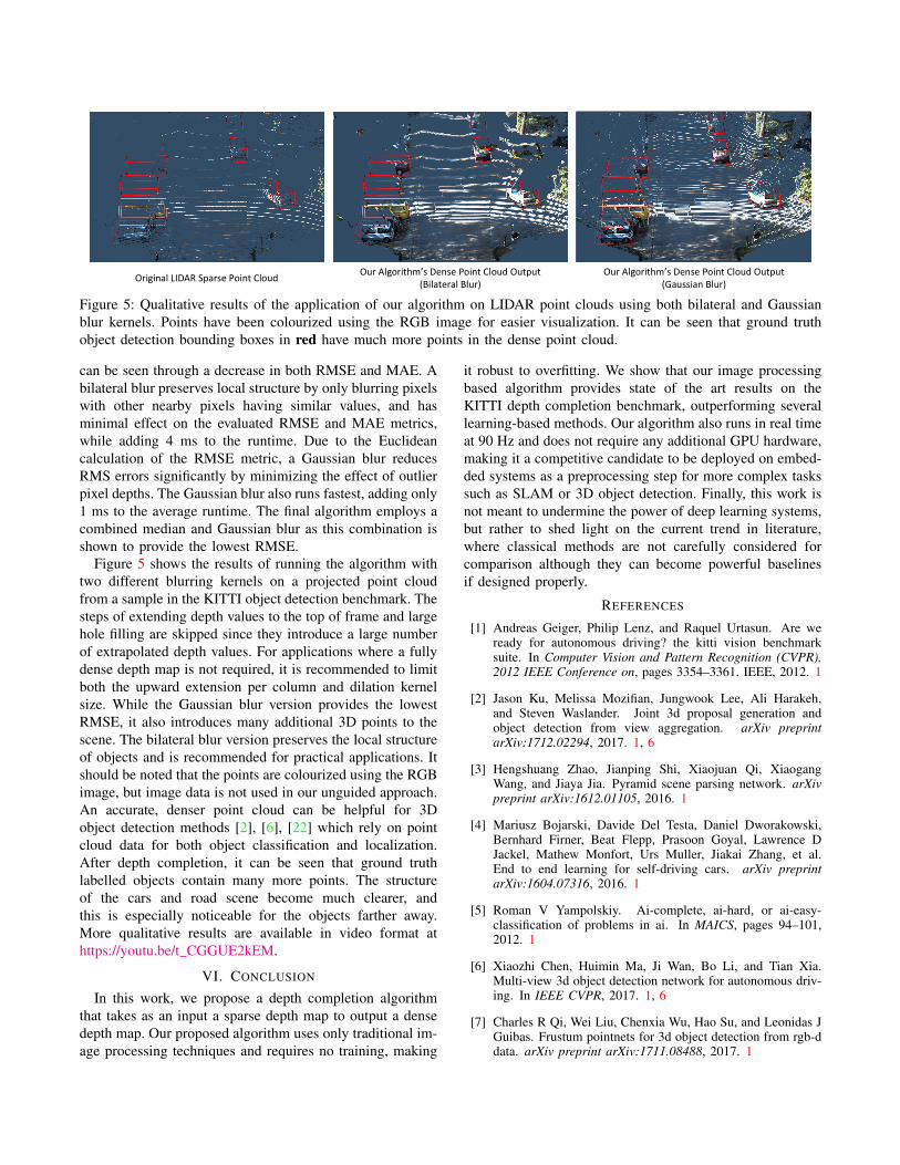
Figure 5: Qualitative results of the application of our algorithm on LIDAR point clouds using both bilateral and Gaussianblur kernels. Points have been colourized using the RGB image for easier visualization. It can be seen that ground truthobject detection bounding boxes in red have much more points in the dense point cloud.

can be seen through a decrease in both RMSE and MAE. Abilateral blur preserves local structure by only blurring pixelswith other nearby pixels having similar values, and hasminimal effect on the evaluated RMSE and MAE metrics,while adding 4 ms to the runtime. Due to the Euclideancalculation of the RMSE metric, a Gaussian blur reducesRMS errors significantly by minimizing the effect of outlierpixel depths. The Gaussian blur also runs fastest, adding only1 ms to the average runtime. The final algorithm employs acombined median and Gaussian blur as this combination isshown to provide the lowest RMSE.

Figure 5 shows the results of running the algorithm withtwo different blurring kernels on a projected point cloudfrom a sample in the KITTI object detection benchmark. Thesteps of extending depth values to the top of frame and largehole filling are skipped since they introduce a large numberof extrapolated depth values. For applications where a fullydense depth map is not required, it is recommended to limitboth the upward extension per column and dilation kernelsize. While the Gaussian blur version provides the lowestRMSE, it also introduces many additional 3D points to thescene. The bilateral blur version preserves the local structureof objects and is recommended for practical applications. Itshould be noted that the points are colourized using the RGBimage, but image data is not used in our unguided approach.An accurate, denser point cloud can be helpful for 3Dobject detection methods [2], [6], [22] which rely on pointcloud data for both object classification and localization.After depth completion, it can be seen that ground truthlabelled objects contain many more points. The structureof the cars and road scene become much clearer, andthis is especially noticeable for the objects farther away.More qualitative results are available in video format athttps://youtu.be/t CGGUE2kEM.

VI. CONCLUSION

In this work, we propose a depth completion algorithmthat takes as an input a sparse depth map to output a densedepth map. Our proposed algorithm uses only traditional im-age processing techniques and requires no training, making

it robust to overfitting. We show that our image processingbased algorithm provides state of the art results on theKITTI depth completion benchmark, outperforming severallearning-based methods. Our algorithm also runs in real timeat 90 Hz and does not require any additional GPU hardware,making it a competitive candidate to be deployed on embed-ded systems as a preprocessing step for more complex taskssuch as SLAM or 3D object detection. Finally, this work isnot meant to undermine the power of deep learning systems,but rather to shed light on the current trend in literature,where classical methods are not carefully considered forcomparison although they can become powerful baselinesif designed properly.

REFERENCES

[1] Andreas Geiger, Philip Lenz, and Raquel Urtasun. Are weready for autonomous driving? the kitti vision benchmarksuite. In Computer Vision and Pattern Recognition (CVPR),2012 IEEE Conference on, pages 3354–3361. IEEE, 2012. 1

[2] Jason Ku, Melissa Mozifian, Jungwook Lee, Ali Harakeh,and Steven Waslander. Joint 3d proposal generation andobject detection from view aggregation. arXiv preprintarXiv:1712.02294, 2017. 1, 6

[3] Hengshuang Zhao, Jianping Shi, Xiaojuan Qi, XiaogangWang, and Jiaya Jia. Pyramid scene parsing network. arXivpreprint arXiv:1612.01105, 2016. 1

[4] Mariusz Bojarski, Davide Del Testa, Daniel Dworakowski,Bernhard Firner, Beat Flepp, Prasoon Goyal, Lawrence DJackel, Mathew Monfort, Urs Muller, Jiakai Zhang, et al.End to end learning for self-driving cars. arXiv preprintarXiv:1604.07316, 2016. 1

[5] Roman V Yampolskiy. Ai-complete, ai-hard, or ai-easy-classification of problems in ai. In MAICS, pages 94–101,2012. 1

[6] Xiaozhi Chen, Huimin Ma, Ji Wan, Bo Li, and Tian Xia.Multi-view 3d object detection network for autonomous driv-ing. In IEEE CVPR, 2017. 1, 6

[7] Charles R Qi, Wei Liu, Chenxia Wu, Hao Su, and Leonidas JGuibas. Frustum pointnets for 3d object detection from rgb-ddata. arXiv preprint arXiv:1711.08488, 2017. 1

[8] Derek Chan, Hylke Buisman, Christian Theobalt, and Se-bastian Thrun. A noise-aware filter for real-time depthupsampling. In Workshop on Multi-camera and Multi-modalSensor Fusion Algorithms and Applications-M2SFA2 2008,2008. 1

[9] Jonas Uhrig, Nick Schneider, Lukas Schneider, Uwe Franke,Thomas Brox, and Andreas Geiger. Sparsity invariant cnns.arXiv preprint arXiv:1708.06500, 2017. 1, 2, 4

[10] Kitti Depth Completion Benchmark. http://www.cvlibs.net/datasets/kitti/eval depth.php?benchmark=depth completion.1, 5

[11] Fei Qi, Junyu Han, Pengjin Wang, Guangming Shi, and Fu Li.Structure guided fusion for depth map inpainting. PatternRecognition Letters, 34(1):70–76, 2013. 2

[12] Li Chen, Hui Lin, and Shutao Li. Depth image enhancementfor kinect using region growing and bilateral filter. In PatternRecognition (ICPR), 2012 21st International Conference on,pages 3070–3073. IEEE, 2012. 2

[13] Christian Richardt, Carsten Stoll, Neil A Dodgson, Hans-Peter Seidel, and Christian Theobalt. Coherent spatiotemporalfiltering, upsampling and rendering of rgbz videos. InComputer Graphics Forum, volume 31, pages 247–256. WileyOnline Library, 2012. 2

[14] Sergey Matyunin, Dmitriy Vatolin, Yury Berdnikov, andMaxim Smirnov. Temporal filtering for depth maps gen-erated by kinect depth camera. In 3DTV Conference: TheTrue Vision-Capture, Transmission and Display of 3D Video(3DTV-CON), 2011, pages 1–4. IEEE, 2011. 2

[15] Tak-Wai Hui, Chen Change Loy, and Xiaoou Tang. Depthmap super-resolution by deep multi-scale guidance. InEuropean Conference on Computer Vision, pages 353–369.Springer, 2016. 2

[16] Xibin Song, Yuchao Dai, and Xueying Qin. Deep depth super-resolution: Learning depth super-resolution using deep con-volutional neural network. In Asian Conference on ComputerVision, pages 360–376. Springer, 2016. 2

[17] Michael Hornacek, Christoph Rhemann, Margrit Gelautz, andCarsten Rother. Depth super resolution by rigid body self-similarity in 3d. In Proceedings of the IEEE Conference onComputer Vision and Pattern Recognition, pages 1123–1130,2013. 2

[18] Elizbar A Nadaraya. On estimating regression. Theory ofProbability & Its Applications, 9(1):141–142, 1964. 2

[19] Open Source Computer Vision Library. https://opencv.org/. 3

[20] NumPy. http://www.numpy.org/index.html. 3

[21] James M Coughlan and Alan L Yuille. The manhattanworld assumption: Regularities in scene statistics which en-able bayesian inference. In Advances in Neural InformationProcessing Systems, pages 845–851, 2001. 5

[22] Yin Zhou and Oncel Tuzel. Voxelnet: End-to-end learningfor point cloud based 3d object detection. arXiv preprintarXiv:1711.06396, 2017. 6