Research Collection

Master Thesis

Iterative methods for matrix factorization with missing data

Author(s): Daskalov, Boris Nikolaev

Publication Date: 2011

Permanent Link: https://doi.org/10.3929/ethz-a-006607487

Rights / License: In Copyright - Non-Commercial Use Permitted

This page was generated automatically upon download from the ETH Zurich Research Collection. For moreinformation please consult the Terms of use.

ETH Library

Master Thesis

Iterative Methods forMatrix Factorization with

Missing Data

−1000

100

Author:Boris Nikolaev Daskalov

Supervisor:Marc PollefeysRoland Angst

August 18, 2011

Abstract

This thesis discusses the problem of reconstructing matrices with miss-ing data by utilizing a low-rank constraint. This is an important subprob-lem in structure-from-motion(SFM) tasks in computer vision. It also hasapplications in other fields such as collaborative filtering. This work con-centrates on several algorithms that are commonly used to solve suchproblems: Alternating Least Squares(ALS), Levenberg-Marquardt(LM)and Wiberg’s algorithm(WA). These algorithms were compared on syn-thetic low-rank matrices. Also they were generalized to operate on affinestructure-from-motion(SFM) problems and tested on synthetic and real-world SFM data. The results showed that WA clearly outperforms othermethods by being able to reconstruct the same matrices using less obser-vations. Also for the same number of observations WA converges to theglobal minimum more often and in less iterations than LM and ALS.

Two improvements in the WA are proposed in this thesis. The firstone is a way to apply iterative methods to solve for the step direction.Our approach speeds up the most computationally intensive part of thealgorithm by exploiting the sparsity and the algebraic properties of theproblem. The per-iteration computational complexity of the proposedvariant is similar or lower than the LM algorithm that is commonly usedfor bundle adjustment. It converges faster than LM and finds the globalminimum more often when started from a random point. This makes WApractical to apply to large SFM problems. The other proposed improve-ment is adding soft orthogonality constraints to the optimization problemin a way that preserves the least-squares form of the cost function. Inour experiments this reduced the number of runs that get stuck in a lo-cal minimum and further increased the convergence speed of Wiberg’salgorithm.

1

Contents

1 Introduction 4

2 Notation 6

2.1 Vectorization Operator and Kronecker Product . . . . . . . . . . 6

3 Solving Least-Squares Problems 8

3.1 Definition of a Least-Squares Problem . . . . . . . . . . . . . . . 8

3.2 Solving Linear Least-Squares Problems . . . . . . . . . . . . . . . 8

3.3 Solving Non-Linear Least-Squares Problems . . . . . . . . . . . . 9

4 Low-Rank Matrix Factorization as a Non-Linear Least SquaresProblem 11

4.1 Vectorized formulation . . . . . . . . . . . . . . . . . . . . . . . . 11

4.2 Missing data and noisy observations . . . . . . . . . . . . . . . . 12

4.3 Error function . . . . . . . . . . . . . . . . . . . . . . . . . . . . . 12

4.4 Bi-linearity . . . . . . . . . . . . . . . . . . . . . . . . . . . . . . 13

5 Algorithms 15

5.1 Gauss-Newton based algorithms . . . . . . . . . . . . . . . . . . . 15

5.2 Alternating Least Squares(ALS) . . . . . . . . . . . . . . . . . . 18

5.3 Wiberg’s algorithm . . . . . . . . . . . . . . . . . . . . . . . . . . 19

5.4 Other Algorithms . . . . . . . . . . . . . . . . . . . . . . . . . . . 23

6 Synthetic Experiments 25

6.1 Convergence criteria. . . . . . . . . . . . . . . . . . . . . . . . . . 26

6.2 Plotting the results . . . . . . . . . . . . . . . . . . . . . . . . . . 26

6.3 Results: Base experiment . . . . . . . . . . . . . . . . . . . . . . 27

6.4 Unbalanced singular values . . . . . . . . . . . . . . . . . . . . . 34

6.5 Large rank matrices . . . . . . . . . . . . . . . . . . . . . . . . . 34

7 Application to Affine Structure from Motion problems 38

7.1 Affine factorization model . . . . . . . . . . . . . . . . . . . . . . 38

7.2 Alternating least squares. . . . . . . . . . . . . . . . . . . . . . . 39

7.3 Gauss-Newton based methods. . . . . . . . . . . . . . . . . . . . 40

7.4 Wiberg’s algorithm. . . . . . . . . . . . . . . . . . . . . . . . . . 40

7.5 Orthogonality constraints . . . . . . . . . . . . . . . . . . . . . . 40

7.6 Normalization . . . . . . . . . . . . . . . . . . . . . . . . . . . . . 42

2

8 Experiments on Structure-from-Motion Data 44

8.1 Evaluation on Synthetic SFM Data . . . . . . . . . . . . . . . . . 44

8.2 Evaluation on Real-World SFM Data . . . . . . . . . . . . . . . . 46

9 Conclusion 50

3

1 Introduction

This thesis discusses the problem of low-rank matrix factorization in the pres-ence of missing data. This problem appears in the context computer vision asthe central step in structure-from-motion(SFM) tasks. Another applications in-clude collaborative filtering and illumination based reconstruction. The problemis also related to principal component analysis with missing data.

Structure from motion is the problem of simultaneously deriving the 3D struc-ture of the scene and the motion of the camera over multiple views. Usuallyin such tasks the input consists of the trajectories of multiple scene features asobserved in all or part of the views.

In [11] Tomasi and Kanade discussed a model in which the feature trajectoriesare fully observed and orthographic camera model is assumed. They showed thatunder those conditions the matrix of feature trajectories has rank three becauseit can be decomposed as the product two factors. One of them contains thestacked camera projection matrices and the other - the stacked feature pointcoordinates. The best, in least squares sense, rank-three decomposition of amatrix can be easily reconstructed using singular value decomposition. Thenthe factorization can be used to recover the structure and motion parameters.The Tomasi-Kanade factorization model has been generalized to affine (Poelmanand Kanade[8]) and projective cameras(Sturm and Triggs[10]).

The main problem in factorization based approaches to SFM is handling miss-ing data. Feature trajectories are usually constructed using tracker algorithmswhich are prone to errors. Even if the tracker is perfect a feature can be occludedin some of the views which makes it impossible to track and leads to incompletetrajectories. Usually similar sets of features are observed in consecutive viewsand this causes SFM problems to have a specific observation structure wheremost of the observed entries are located close to the main diagonal of the matrix.

Because of the missing data problem, a popular approach to SFM problems is tocreate partial reconstructions from consecutive two- or three-view problems and”stitch” them together. This ”stitched” solution is later refined to a globallyoptimal solution through the so called bundle adjustment process which usuallyuses the Levenberg-Marquardt(LM) algorithm. This standard approach to SFMis analogous to running an iterative method for matrix factorization with agood initial guess. In this work we will assume that such initial guess is notavailable and explore when factorization algorithms can recover the underlyingstructure without it. We will compare Levenberg-Marquardt, which is a genericalgorithm for least-squares problems, to Alternating Least Squares and Wiberg’salgorithm, which are specialized methods for low-rank matrix factorization. Themain goal of this thesis is to explore the effect of missing data on the algorithmsthat are commonly used to solve low-rank factorization problems. The mainquestion is how does their performance depend on the quantity of observedmatrix entries. Another question that we tried to address is what is the influenceof the diagonal structure that is typical for SFM problems on the performanceof the algorithms.

The structure of this thesis is the following:

• Sec. 2 describes the notation that is used in the rest of the thesis.

4

• Sec. 3 gives a short overview of the methods that are commonly used tosolve linear and non-linear least-squares problems.

• Sec. 4 explains how matrix factorization is defined as least-squares mini-mization problem and shows some of its properties.

• Sec. 5 defines the algorithms that were compared in the experiments.

• Sec. 6 describes the experiments on synthetic low-rank matrices and dis-cusses the results from them.

• Sec. 7 explains the connection between low-rank matrix factorization andSFM problems and shows how the algorithms presented in Sec. 5 can begeneralized to operate on affine SFM data.

• Sec. 8 presents experiments on synthetic and real-world SFM data anddiscusses the results.

5

2 Notation

In this work vectors will be noted with bold lower-case letters and matriceswith bold upper-case letters. The sizes of matrices will be given as a subscriptsometimes(e.g. Am×n). The identity matrix of size n×n will be denoted as In.

The size may be omitted in some cases. PA = A(ATA)−1

AT is a projectionto the column space of the matrix A and QA = I − PA is a projection to thecolumn space orthogonal to the column space of A. An orthogonal basis ofthe column space of A will be denoted as OA.

∥∥A∥∥F

denotes the Frobenius

norm of the matrix A and∥∥x∥∥

2- the 2-norm of the vector x. 0 stands for the

zero vector and 1 for the vector with all elements equal to one. All vectors arecolumn-vectors.

2.1 Vectorization Operator and Kronecker Product

In this work we will need to treat matrices as elements of a linear space and willuse the vectorization operator vec [A]. This operator constructs a vector froma matrix by concatenating all the columns as follows:

vec

a1,1 a1,2 · · · a1,n

a2,1 a2,2 · · · a2,n

......

. . ....

am,1 am,2 · · · am,n

=

a1,1

...am,1a1,2

...am,n

(1)

The Kronecker product denoted by ⊗ is a matrix-matrix operation defined as:

Am×n ⊗Bp×q =

a11B . . . a1nB...

. . ....

am1B . . . amnB

mp×nq

(2)

There is an important connection between the vectorization operator and theKronecker product:

vec [AXB] = (BT ⊗A) vec [X] (3)

This property allows us to rearrange a matrix-matrix product as a matrix vectorproduct as follows:

vec [AX] = vec [AXI] = (I ⊗A) vec [X] (4)

vec [XA] = vec [IXA] = (AT ⊗ I) vec [X] (5)

This is especially useful when derivatives of matrices have to be computed.Using vectorization one can calculate the derivative of a matrix with respect toanother matrix by reshaping both matrices as vectors and taking the Jacobian.

Some other properties of the Kronecker product that will be used are:

6

• Bi-linearity:(A + B)⊗C = (A⊗C) + (B⊗C) (6)

A⊗ (B + C) = (A⊗B) + (A⊗C) (7)

λ(A⊗B) = (λA)⊗B = A⊗ (λB) (8)

• Mixed-product property:

(A⊗B)(C⊗D) = AC⊗BD (9)

when the products AC and BD can be formed.

• Transposition:(A⊗B)T = AT ⊗BT (10)

• Inversion:(A⊗B)−1 = A−1 ⊗B−1 (11)

Another matrix-matrix operation that will be used is the element-wise or Hadamardproduct denoted by �. It is defined as:

Am×n �Bm×n =

a11b11 . . . a1nb1n...

. . ....

am1bmn . . . amnbmn

m×n

(12)

7

3 Solving Least-Squares Problems

Linear and non-linear least-squares(LS) problems are central building blocksfor the methods that will be presented. This section is a brief introduction toLS problems and algorithms for solving them. If the reader is familiar withthat material it can be safely skipped as it does not include anything specificto matrix factorization. More comprehensive discussion of the material in thissection can be found in [6].

3.1 Definition of a Least-Squares Problem

A least-squares problem is defined as:

minx

F (x)

where F (x) =

m∑i=1

r2i (x)

(13)

Such problems often arise when fitting a model to a set of observations in away that minimizes the sum of squared errors. Typically each function ri(x)represents the difference between predicted and observed values for one datapoint. The vector r(x) = [r1(x) r2(x) . . . rm(x)] is called residual vector.A least squares problem can be formulated in terms of the residual vector asfollows:

minx

F (x)

where F (x) =∥∥r(x)

∥∥2

2= rT (x)r(x)

(14)

A necessary but not sufficient condition for x to be a solution of a LS problemis the following:

0 =∂F (x)

∂x= 2

∂r(x)

∂x

T

r(x) (15)

We will note the Jacobian ∂r(x)∂x with J and write to optimality condition as:

JT r = 0 (16)

3.2 Solving Linear Least-Squares Problems

In cases where r(x) is a linear function:

r(x) = Ax− b (17)

the Jacobian is:

J =∂r

∂x= A (18)

and the corresponding optimality condition is:

AT (Ax− b) = 0 (19)

8

ATAx = ATb (20)

This system can be solved to x = (ATA)−1

ATb provided that A has a fullrank. If A is rank deficient there is a linear subspace of equivalent solutionsthat have the same cost function value.

In practice inverting the matrix ATA or solving the normal equations (20) iscomputationally expensive and numerically unstable. This is why LLS problemsare usually solved using QR decomposition. The complexity of solving a denseLLS problem with m equations and n variables using QR is O(mn2).

In cases where the matrix A is sparse the speed can be improved by usingiterative methods like CGLS or LSQR. Such methods need only subroutines thatmultiply an arbitrary vector by A or AT . These multiplications need time that isproportional to the number of non-zero elements of A. The number of matrix-vector multiplications needed in the worst case is O(n). The complexity ofsolving a sparse LLS problem is O(ln) where l is the number of non-zero entriesin A. It is important to note that O(n) multiplications is a very pessimisticbound and these methods usually reach a satisfactory solution much faster.

3.3 Solving Non-Linear Least-Squares Problems

Solvers for non-linear least-squares problems are usually based on the Gauss-Newton algorithm. This method needs a starting point x0. Then it creates alocal linear approximation of the residual around r(x0):

r(x0 + ∆x) ≈ r(x0) + J(x0)∆x (21)

The next step is to solve the linear least squares problem:

∆x = argmin∆x

∥∥r(x0) + J(x0)∆x∥∥2

2(22)

The solution ∆x is a descent direction for F (x). After computing it the algo-rithm performs a step in this direction. It is important to control the step sizesince this guarantees that the function value will decrease and that the algo-rithm will converge. Different Gauss-Newton based methods differ mostly intheir approach to controlling the step size. There are three methods to do that:

• Line searchThis method solves a one dimensional optimization problem to determinea good step size. It finds a local minimum on the line defined by thecurrent point and the descent direction. Generally this is done using onedimensional black-box optimization like golden-ratio search, but in somecases it is possible to perform the line search analytically.

• Levenberg-MarquardtThis approach extends the Gauss-Newton algorithm by adding a step-sizepenalty when solving for the step direction in (22). The regularizationparameter is changed dynamically. Effectively this leads to interpolationof the step direction between the GN direction and the direction of steepestdescent.

9

• Trust regionsThis is another approach that interpolates between the GN direction andthe direction of steepest descent. It does not regularize the optimizationproblem (22) but defines a region in which it is trusted to be a good ap-proximation. The size of the region is dynamically modified. This methodis very similar to Levenberg-Marquardt although there is no analyticalconnection between them.

10

4 Low-Rank Matrix Factorization as a Non-LinearLeast Squares Problem

The main subject of this work is the problem of recovering a matrix Xm×n witha given low rank k � m < n. The low rank constraint implies that X can berepresented as a product of two matrices Um×k and Vk×n such that:

Xm×n = Um×kVk×n (23)

If we note the columns of V with {vj}j=1..nthen the j-th column of X is equal

to Uvj . Each column of X is a linear combination of the columns of U withcoefficients vj . This means that U is a basis of the column space of X. SimilarlyV is a basis of the row space of X.

Of course this representation is not unique. There are multiple bases of therow and column spaces of X. Actually for each invertible matrix Qk×k one cancreate an equivalent factorization:

Xm×n = U′m×kV′k×n

where

U′m×k = Um×kQk×k

V′k×n = Q−1k×kVk×n

(24)

Because of this ambiguity, the factorization has mk+nk−k2 degrees of freedom.For small values of k this is much smaller than the number of degrees of freedomof X which is mn. This makes it possible to recover the full matrix X byobserving only a subset of its elements.

4.1 Vectorized formulation

The set of matrices with fixed size is a linear space. When fitting our model toobservations it is useful to treat X, U or V as vectors of such linear space. Itis convenient to have a way of writing the problem in which their elements arearranged in vectors. This can be achieved easily using the Kronecker productproperty of the vectorization operator.

vec [X] = vec [UV]

= (VT ⊗ Im) vec [V]

= (In ⊗U) vec [U]

(25)

This is an equivalent representation of a low rank matrix factorization whichis much more convenient to work with when fitting the model to data. In thisthesis both representations will be used depending on which is more suitable forthe particular situation. The matrix formulation is easier to interpret, whereasthe vectorized formulation is useful since most optimization algorithms expectthe parameters to be arranged in a vector and need to compute derivatives.

11

4.2 Missing data and noisy observations

We will assume that there is a ground truth matrix Xm×n which we are tryingto reconstruct and which has a known low rank k. Our input data consists ofthe matrices Xm×n and Mm×n such that:

X = M� (X + noise) (26)

M is a boolean mask over that selects an observed subset of the elements. Thismeans that if mij = 1 then the corresponding element xij is observed andxij = xij + ηij where ηij is a noise term. Since Xm×n has a fixed low rank k, itcan be factorized into Um×k and Vk×n:

X = UV

X = M� (UV + noise)

X,X ∈ Rm×nU ∈ Rm×rV ∈ Rr×n

(27)

The goal is to recover X by finding a factorization UV that explains the elementsobserved in X.

For the vectorized formulation, instead of masking, one can create a vector thatcontains only the observed elements of vec

[X]. We will note this vector with

x. x and X are related by the following equations:

x = S vec[X]

vec[X]

= STx(28)

S is a matrix that discards the unnecessary elements of vec[X]

(those thatare removed by the zero elements of M). It is also possible to do the reverseoperation in which we fill in the missing elements by zeros by multiplying withthe transpose of S. S is such that its rows are a subset of the rows of the identitymatrix and it is functionally dependent on M.

For convenience we will use the following notation:

F = S(VT ⊗ Im)

G = S(In ⊗U)

u = vec [U]

v = vec [V]

x = S vec [X]

(29)

This way the model is formulated as:

x = F u = G v (30)

4.3 Error function

For the sake of simplicity we assume that the noise is i.i.d. Gaussian and it’smagnitude is small. In such models the maximum likelihood solution is givenby the global minimum of the least squares error function:

12

E(U,V) =∥∥M� (UV −X)

∥∥2

F(31)

We can also define the error function in the terms of the residual matrix:

R = M� (UV −X) (32)

E(U,V) =∥∥R∥∥2

F(33)

A corresponding definition for the vectorized model is:

r = Fu− x = Gv − x (34)

e(u,v) =∥∥r∥∥2

2= rT r (35)

A summary of the values involved in the definition of the error function andthe connections between the matrix and vector formulations can be found inTab. 4.4.

It is important to note that minimizing the l2 norm of the error is not theoptimal choice for all applications. It is particularly not suitable for cases wherethere are outliers in the training examples. Robust cost functions are often usedin practice in order the reduce the effect of outliers on the final solution. Anexample of a matrix factorization method that minimizes l1 norm in order tobe robust to outliers can be found in [2].

4.4 Bi-linearity

An important feature of the model is that it is linear in both U and V. Thismeans that one can find an optimal closed form solution for U given V. Moreprecisely we have a linear least-squares problem in u or v and the closed formsolution is given by multiplying with the pseudo-inverse of F or G.

vec[U]

= u = (FTF)−1

FTx (36)

vec[V]

= v = (GTG)−1

GTx (37)

13

Mat

rix

form

ula

tion

Vec

tori

zed

form

ula

tion

Con

nec

tion

Row

sm

Col

um

ns

nR

ank

kO

bse

rved

elem

ents

lG

rou

nd

tru

thX

xx

=S

vec

[X]

Low

-ran

km

od

elU

,Vu

,vu

=ve

c[U

],v

=ve

c[V

]O

bse

rvat

ion

sX

xx

=S

vec[ X]

Mas

k/

Pro

ject

ion

MS

Res

idu

alR

=M�

(UV−

X)

r=

Fu−

x=

Gv−

xr

=S

vec

[R]

Err

orfu

nct

ion

E(U,V

)=∥ ∥ R∥ ∥

2 Fe(

u,v

)=∥ ∥ r∥ ∥2 2

e(ve

c[U

],ve

c[V

])=

E(U,V

)

Tab

le1:

Nota

tion

refe

ren

ce.

14

5 Algorithms

Sec. 4 defined the task of fitting a low-rank factorization to a partially observedmatrix as a non-linear least squares problem. Such problems are most com-monly solved by algorithms that are based on the Gauss-Newton method. Ourparticular problem has a specific structure that can be exploited in order tospeed up such generic methods. In this section we will describe how this can beaccomplished. Also we will look into some methods that are specific to the low-rank factorization task like Alternating Least Squares and Wiberg’s algorithm.In the end we will give a quick overview of some other methods that are usedmostly for collaborative filtering problems and as our experiments have showndo not perform that well for matrix factorizations that represents structure frommotion tasks.

5.1 Gauss-Newton based algorithms

Gauss-Newton is a generic method for non-linear least squares problem. In eachiteration it constructs a linear approximation of the residual around the currentvalue of the parameters x:

r(x + ∆x) ≈ r(x) +∂r(x)

∂x∆x (38)

Then it solves the linear least squares problem:

argmin∆x

∥∥∥r(x) + ∂r(x)∂x ∆x

∥∥∥2

2(39)

Then the algorithm makes a step in the direction defined by ∆x, which isguaranteed to be a descent direction. There are various ways to select the stepsize in a way that ensures that the value of the cost function will be lower inthe next iteration.

5.1.1 Solving for the step direction

As defined in (34) the residual of the matrix factorization problem is:

r = Fu− x = Gv − x (40)

Since r is linear in u and v separately, the Jacobians with respect to them areobviously:

Ju =∂r

∂u= F (41)

Jv =∂r

∂v= G (42)

In order to apply the GN algorithm, one must combine the parameters in a single

vector. We chose to stack u and v vertically as

[uv

]. This way the Jacobian

15

with respect to the full parameter vector is the horizontal concatenation of Juand Jv:

J =[Ju Jv

]=[F G

]=[S(VT ⊗ Im) S(In ⊗U)

]= S

[VT ⊗ Im In ⊗U

] (43)

The next step is to solve the overdetermined linear system J

[∆u∆v

]= −r in least

squares sense. It is important to take into account the fact that J =[F G

]and F and G have exactly lk non-zero elements each. So J has only 2lk non-zero elements out of l(m + n)k and using a sparse least squares solver for thisstep leads to a much more efficient implementation. There are two types ofsuch solvers: direct and iterative. Direct algorithms for solving linear systemsoperate on the matrix that defines the system. On the other hand iterativesolvers only need an user-supplied procedure that multiplies an arbitrary vectorby J or its transpose. Because of the specific structure of the Jacobian thesemultiplications can be done without explicitly constructing J.

When doing the multiplication Jy, one can interpret y as a change in theparameters:

y =

[∆u∆v

]Jy = S

[VT ⊗ Im In ⊗U

] [∆u∆v

]= S((VT ⊗ Im)∆u + (In ⊗U)∆v)

= S((VT ⊗ Im) vec [∆U] + (In ⊗U) vec [∆V])

= S(vec [∆U V] + vec [U ∆V])

= S vec [∆U V + U ∆V]

= S vec [M� (∆U V + U ∆V)]

(44)

This can be computed in O(lk) time if one does not compute the whole matrices∆UV and U ∆V but only the elements that are observed (the ones that arenot masked by M). This is actually the same complexity as multiplying by asparse version of J but it does not require constructing it explicitly.

Similarly, when computing JTy, one can interpret y as as a change in the

16

residual:

y = ∆r

STy = vec [∆R]

JTy = (S[VT ⊗ Im In ⊗U

])Ty

=

[V ⊗ ImIn ⊗UT

]STy

=

[V ⊗ ImIn ⊗UT

]vec [∆R]

=

[(V ⊗ Im) vec [∆R](In ⊗UT ) vec [∆R]

]=

[vec[∆R VT

]vec[UT ∆R

]]

(45)

Since ∆R has only l non-zero elements, this operation also has complexity O(lk).

5.1.2 Line search

The simplest way to determine a step size that ensures that the value of the costfunction will decrease is to perform a search on the line defined by the current

point and the direction

[∆u∆v

]. More precisely, one has to solve the following

problem:

argminλ

∥∥M� ((U + λ∆U)(V + λ∆V)−X)∥∥2

F(46)

Usually line search uses a black-box style minimization method like golden-ratiosearch. In [5] Hartley and Schaffalitzky show that for any given line the costfunction is a 4th degree polynomial. This can be used to perform the line searchanalytically. Line search can be reformulated as:

argminλ

P (λ)

where

P (λ) =∥∥M� ((U + λ∆U)(V + λ∆V)−X)

∥∥2

F

=∥∥M� (UV −X + λ(U∆V + ∆UV) + λ2∆U∆V)

∥∥2

F

=∥∥M� (A + λB + λ2C)

∥∥2

F

=∑

(i,j)|mij=1

(aij + λbij + λ2cij)2

and

A = UV −X

B = U∆V + ∆UV

C = ∆U∆V

(47)

17

P (λ) =∑

(i,j)|mij=1

(aij + λbij + λ2cij)2

=∑

(i,j)|mij=1

(a2ij + λ2b2ij + λ4c2ij + 2λaijbij + 2λ2aijcij + 2λ3bijcij)

=∑

(i,j)|mij=1

(a2ij + 2aijbijλ+ (b2ij + 2aijcij)λ

2 + 2bijcijλ3 + c2ijλ

4)

= λ0∑

(i,j)|mij=1

a2ij

+ λ1∑

(i,j)|mij=1

2aijbij

+ λ2∑

(i,j)|mij=1

(b2ij + 2aijcij)

+ λ3∑

(i,j)|mij=1

2bijcij)

+ λ4∑

(i,j)|mij=1

2c2ij)

(48)

So P (λ) is a polynomial of degree 4 that can be easily minimized. Calculatingthe coefficients of P (λ) can be done in O(lk) time. This is much faster thangolden-ratio search and other black-box optimization routines, that require mul-tiple evaluations of the cost function, each of which costs O(lk) steps.

5.1.3 Levenberg-Marquard and Trust-Region-Reflective

We also created implementations based on the Levenberg-Marquardt and Trust-Region-Reflective algorithms available in the MATLAB optimization toolbox.Both of these algorithms extend Gauss-Newton by evaluating the quality of thelinear approximation and dynamically adjusting the step size and direction inorder to guarantee that the function value will decrease without performing linesearch. In terms of recovery rate all the approaches(GN with line search, LMand TRR) performed similarly. This is why we chose to present only the resultsfor the Levenberg-Marquardt method, which is also the most popular non-linearleast squares approach used for bundle adjustment in computer vision. A prob-lem in MATLAB’s implementation of LM is that it is hard-coded to use a directsolver for the step direction. For the relatively small problem sizes in most ofthe experiments this did not cause a significant slowdown but for our tests onlarge-rank matrices we had to use TRR instead. All three implementations areavailable in the source code package that is part of this thesis.

5.2 Alternating Least Squares(ALS)

ALS is an application of the coordinate descent method for low-rank factor-ization problem. More specifically, ALS is a cyclic block-coordinate descentmethod. It alternatively optimizes the values of U and V while keeping the

18

other one fixed and can be implemented as alternating applications of equations(36) and (37). See Alg. 1.

Algorithm 1 Alternating Least Squares: Naive version

1: Initialize u and v.2: repeat

3: u← u = (FTF )−1FTx

4: v← v = (GTG)−1GTx

5: until converged

A more efficient version(Alg. 2) decomposes the update in steps 3 and 4 intoseveral smaller linear least-squares problems. A key observation is that theelements in the i-th row of X depend only on the i-th row of U and the matrixV. This means that one can solve for each row of U independently using astandard linear-least squares solver. Missing elements are handled by maskingthe corresponding elements of xi,: and columns of V. Analogously one can findthe optimum for each column of V independently. When solving for the rowsof U we have m independent linear least squares problems of sizes li× k, whereli is the number of observed elements in the i-th row. The i-th problem hascomplexity O(lik

2). Since l =∑i li, the time required to compute U is O(lk2).

Analogously the time for computing the optimal value of V is also O(lk2).

Algorithm 2 Alternating Least Squares: Optimized version

1: Initialize U and V.2: repeat3: for i = 1 to m do4: mask ← indexes of observed elements in the i-th row of X5: ui: ← lsqlin(VT

:,mask , Xi,mask)6: end for7: for j = 1 to n do8: mask ← indexes of observed elements in the j-th column of X9: v:j ← lsqlin(Umask,: , Xmask,j)

10: end for11: until converged

5.3 Wiberg’s algorithm

Wiberg’s algorithm is an instance of the variable projection method specializedfor low-rank matrix approximation. The variable projection method is a methodfor solving least-squares problems in which the model is linear in part of theparameters. More details about it can be found in [3].

In the case of low-rank matrix approximation the model is linear in both uand v separately. When applying a variable projection method one can decidewhich part of the parameters are to be dropped. Due to the importance of theWiberg algorithm in our experiments, we provide a detailed derivation of thisalgorithm. The derivation follows closely the presentation in [7]. Although weuse a similar notation, we parametrize the cost function using u while Okatani

19

and Deguchi use v. This is entirely a notation difference and the two derivationsare equvalent.

Derivation of the Inner LS-Problem

The main point in this algorithm is the re-parametrization of the cost function.From (37) you know that for all local minima of e(u,v) it holds that v = v(u),where v(u) is the least squares solution for v for the given u. This allows usto restrict the optimization procedure to work on the subspace defined by thisequation. This leads to two equivalent ways of writing the optimization problemthat we are solving. The first one is:

minimize e(u,v)

s.t. v = v(u) = (GTG)−1

GTx(49)

An alternative view is that we are minimizing a modified cost function:

ε(u) = e(u, v(u))

= ρTρ

=∥∥ρ∥∥2

2

(50)

where ρ is the residual as a function of u:

ρ = Gv − x

= −(I −G(GTG)−1

GT )x

= −QGx

(51)

QG is a projection to the subspace orthogonal to the columns of G.

The Wiberg algorithm uses Gauss-Newton steps to optimize the cost functionρ and needs to compute the Jacobian ∂ρ

∂u , which is not the same as ∂r∂u . The

connection between the them is given by:

J =∂ρ

∂u=∂r

∂u+∂r

∂v

∂v

∂u(52)

We know that ∂r∂v = F and ∂r

∂u = G. The problem is computing ∂v∂u . In order

to do that we will look at the the partial derivative of the original cost functione(u,v) with respect to v. Let f(u,v) = ∂e

∂v :

f(u,v) =∂e

∂v

=∂(rT r)

∂v

= 2∂r

∂v

T

r

= 2GT r

= 2GT (Gv − x)

= 2GT r(u,v)

(53)

20

The construction of v(u) ensures that:

φ(u) = f(u, v(u)) = 0 ∀u (54)

φ(u) = 2GTρ(u) (55)

So φ which is a function of u is the constant zero. This implies that its Jacobianwith respect to u must be zero:

0 =∂φ

∂u=∂GTρ(u, v)

∂u=∂G

∂u

T

ρ+ GT ∂ρ

∂u(56)

In the spirit of the Gauss-Newton algorithm, one can assume that the norm of

the residual ρ is small and drop the term ∂G∂u

Tρ.

0 ≈ GT ∂ρ

∂u

0 ≈ GT (∂r

∂u+∂r

∂v

∂v

∂u)

0 ≈ GT (F + G∂v

∂u)

(57)

It follows that:dv

du≈ −(GTG)

−1GTF (58)

Which can be substituted in (52) in order to get and approximate formula forthe Jacobian:

J =∂r

∂u+∂r

∂v

∂v

∂u

= F + G∂v

∂u

≈ F + G(−(GTG)−1

GTF) = (I −G(GTG)−1

GT )F

= QGF

(59)

Having calculated the residual in (51) and the approximate Jacobian in (59) onecan perform a Gauss-Newton step. The increment is computed by solving:∥∥J∆u + r

∥∥2→ min (60)

Which is equivalent to: ∥∥QGF∆u−QGx∥∥

2→ min (61)

In [7] Okatani and Deguchi prove that the matrix QGF is rank deficient withrank at most (m − k)k. This means that there exists a linear subspace ofequivalent least squares solutions. Since the solution represents a step and thesystem is a local approximation of the original problem, it is reasonable to limitthe norm of the step in some way. This leads to various ways to regularize theproblem.

21

Solving the Inner LS-Problem

The size of this least squares problem is l×mk. A typical large structure-from-motion problem can have thousands of rows m and millions of observations l.This is why solving for the step direction is usually the most compute-intensivepart of the algorithm and requires special attention.

Okatani and Deguchi recommend using the Moore-Penrose pseudo-inverse tosolve this problem. In an under-determined system, multiplying with the pseudo-inverse leads to the solution that has minimal l2 norm. This can be computedusing the truncated SVD of the Jacobian. The problem with this approach isthat computing the SVD requires O(l2mk+ lm2k2) steps which makes it unfea-sible for large problems. An implementation that uses QR decomposition has acomplexity O(lm2k2) which is a lot faster but still has a quadratic dependenceon m.

Instead we used LSQR, which is an iterative method for solving linear least-squares problems. It does not require explicit representation of the matrix butonly procedures that multiply by the Jacobian and its transpose. Since F and Gare sparse these multiplication can be computed efficiently as several successivesparse matrix-vector multiplications. One can decompose the multiplicationJ∆u into two successive matrix-vector multiplications: QG(F∆u). The firstone F∆u takes O(lk) steps due to the sparsity of F. Let z = F∆u. QG is aprojection to the subspace orthogonal to the column space of G. From this:

QGz = (Il −PG)z = z−PGz (62)

where PG is the projector to the column space of G. But G has a block diagonalstructure and can be orthogonalized in O(lk2) steps because each block can beorthogonalized separately from the others. An orthogonal basis can be easilyassembled from the individual orthogonal bases of the blocks. Let OG be anorthonormal basis of the column space of G. Then:

QGz = z−PGz = z−OGOTGz (63)

and this can be computed inO(lk) steps. OG does not change between iterationsof the LSQR algorithm and can be precomputed. This way the complexity ofone LSQR iterations is O(lk).

In [4] Hanke shows that iterative methods like LSQR and CGLS can be usedto solve ill-conditioned least squares problems and they give solutions similarto the ones obtained by truncated SVD. The key point is that these methodshave the so-called semi-convergence property. They initially converge to thesolution and later diverge driven by the noise and numerical errors. This meansit is important to terminate the iterations early enough. Hanke observed thatthe number of iterations is in practice smaller than the optimal number ofcomponents of the truncated SVD. That is why we chose to run LSQR for amaximum of (m−k)k iterations. We do not have a hard theoretical justificationfor this number but we have observed in experiments that it works at least aswell as the truncated SVD approach. Each Wiberg outer iteration is limited toO(m − k)k internal LSQR iterations and each of them has complexity O(lk).Computing OG takes additional O(lk2) operations per outer iteration. Thus thecomplexity of one Wiberg outer iteration in our implementation is O(lmk2).

22

In practice the LSQR algorithm reaches the needed precision and the inneriterations stop early so this bound is actually pessimistic.

Line Search

As described in [7], Wiberg’s algorithm does not include any form of step sizecontrol. This allows the algorithm to do steps that increase the value of thecost function. Unfortunately the scheme for doing the line search analytically,presented in Sec. 5.1.2, can not be used for this model because v(u) is a non-linear function. We added a line search procedure using MATLAB’s built-infunction ”fminunc”, which generally reduces the number number of iterationsat the cost of making each iteration more expensive. The cost of a line searchcan be significant since the complexity of evaluating the cost function at asingle point is O(lk2). In practice adding line search can double the time periteration, which may not justify the savings in the number of iterations. Weused it because it is the simplest way to ensure that the algorithm will converge,although a trust-region based approach may be faster.

Algorithm 3 Wiberg’s algorithm

1: Initialize u.2: repeat3: G← S(In ⊗U)4: v← v(u,x) (computed in the same way as in Alg. 2)5: F← S(VT ⊗ In)6: OG ← orth(G)7: rhs← x−OG(OT

Gx)8: ∆u← LSQR(Jmultfunc, JTmultfunc, rhs)9: α = argminα ε(u + α∆u)

10: u← u + α∆u11: until converged

Algorithm 4 Jmultfunc

1: z← Fx2: return z−OG(OT

Gz)

Algorithm 5 JTmultfunc

1: return FT (x−OG(OTGx))

5.4 Other Algorithms

In the process of preparing this thesis we looked into several other algorithms.The topic of low-rank matrix factorization is especially popular in the collabo-rative filtering community. We tried two methods that have been successfullyused to train a factorized model of the Netflix dataset. Both methods performedworse than the approaches that were described and this is why we left them out

23

of the comparison. We include a short description of our observations for thesake of completeness. Implementations are included in the source code packagethat is part of this thesis.

Gradient Descent and Stochastic Gradient Descent(SGD)

Gradient descent performs a line search in the direction of steepest descent(JT rfor least squares problems). This can be computed very efficiently - O(lk).

SGD uses a single data point error function. In each iteration it samples fromthe empirical distribution of the data and makes a small step in the oppositedirection of the gradient. The size of the step is controlled by a ”learning rate”parameter. Because a single data point depends only on one row of U and onecolumn of V the cost of such a step is O(k). This also makes the algorithmreally fast and simple to program.

Both Gradient descent and SGD had similar but worse recovery rates and con-vergence speed than Alternating Least Squares. This why we decided to leavethem out of the comparison. However, both algorithms have the advantageof being linear in the rank parameter instead of quadratic. (O(lk) instead ofO(lk2)). This may be an advantage when constructing factorizations of a largerrank. For structure from motion problems the rank is usually 3 or 4 and this isnot really an advantage.

Bayesian Probabilistic Matrix Factorization

Bayesian Probabilistic Matrix Factorization by Salakhutdinov and Mnih([9]) isa probailistic model of matrix factorization that can be sampled using MarkovChain Monte Carlo techniques. In the original paper it was sampled usinga Gibbs sampler which loosely resembles cyclic block coordinate descent withsome randomness added in each step. This makes the method very similar toAlternating Least Squares. This was also observed in experiments. Addition-ally in structure from motion tasks one is usually targeting a point estimatefor the camera projection matrices which is incompatible with the set of sam-ples(separate factorizations) that is provided by MCMC.

24

6 Synthetic Experiments

The performance of the algorithms was evaluated on synthetic data. Eachmethod was applied to a set of random low-rank matrices. In each run a subsetof the elements of the random matrix was given as an input to a recovery al-gorithm. The output was interpreted as an attempted recovery of the originalmatrix. Such setup allowed us to compare the results of the algorithms withthe ground truth matrix. The main goals of this evaluation were to answer thefollowing questions:

• How often do different algorithms converge to a the global minimum?

• How much iterations do they need to converge?

• How many observations are necessary in order to recover the original ma-trix reliably?

The random synthetic problems were generated using the following procedure:

Algorithm 6 Create random synthetic experiment.

1: Generate U and V using the full dimensionality (m + n)k. Elements arei.i.d. samples from N (0, 1).

2: Use QR decomposition to orthogonalize and normalize U and VT .3: Set X = USV. Where S is a fixed diagonal matrix containing the singular

values.4: Add normally distributed noise. Xnoise = X + randn(m,n)σnoise.5: Sample the elements of Xnoise to get the observed matrix X.

Using normal distribution in step 1 ensures that the column space of U and therow space of V are uniformly distributed. In step 2 QR decomposition is usedto construct orthonormal bases of those subspaces. Then fixed singular valuesare introduced and the matrix X is constructed. By controlling the singularvalues one can control the magnitude of the matrix elements. It also allowsto construct degenerate cases in which the singular values are unbalanced. In

all experiments we enforced∥∥UV

∥∥2

F= mn by setting the norm of the singular

values vector to√mn. This way the root mean square of the matrix elements

is 1. In the base experiment the magnitude of the noise is σnoise = 0.01 sothat the expected value of RMSE(X,Xnoise) is 0.01. This means that theglobal minimum of the cost function is less than or equal to 0.01 and close to it.This allows to roughly classify if a particular run has converged to the globalminimum(≤ 0.01) or to a local minimum(≥ 0.01).

Two different algorithms were used in the last step to sample matrix elements:

• Uniform sampling.This approach selects, uniformly at random, from all possible subsets ofthe matrix elements with the given size. If a row or a column has lesssamples than the rank of the matrix, additional elements are included byuniformly sampling the not-included elements in the row/column.

25

• Diagonal sampling.This approach samples uniformly in a band around the main diagonal ofthe matrix. This method is designed to simulate an observation patternthat is common in real-world structure from motion data. Our resultsshowed that such observation structure can have significant effects on thechances of some algorithms to recover the original matrix. The methodfirst removes all elements outside the diagonal band and then calls theuniform sampler on the rest of the elements. The band width is selectedto be the minimal possible that has no less than 1.5 times the requestednumber of elements.

The number of observed elements is selected uniformly at random in the range1.1 to 6 observations per degree of freedom. For each fixed values of the pa-rameters(matrix size, rank, singular valus, noise magnitude) 200 test cases weregenerated. Then each algorithm was ran on each test case.

6.1 Convergence criteria.

All algorithms were run for a maximum of 100 iterations or until they converged.A run was considered converged if:

• the root mean squared error(RMSE) measured on the training data is lessthan 10−2 OR

• the change in the RMSE has been lower than 10−5 for 5 consecutive iter-ations.

In general, comparison with limited number of iterations can be misleading sincesome algorithms need more iterations to converge than others. Also some(i.e.ALS) have much lower iterations times than others.That is why we ran a set ofexperiments in which the maximum number of iterations was increased to 1000.This did not lead to a significant change of the results. After 100 iterations,the algorithms converged reasonably close to a minima in most cases and anincreased number of iterations did not change the results considerably. This isdescribed in detail in Sec. 6.3.1.

6.2 Plotting the results

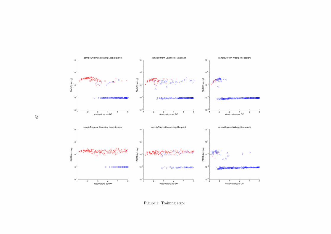
The results are presented as scatter-plots in which each point represents theresult of a single run of a recovery algorithm on a randomly generated problem.The problems and their corresponding initial values are the same for all com-pared algorithms. A blue circle marks a converged run. Red cross means thatthe algorithm was terminated because the maximum number of iterations hadbeen reached.

On the horizontal axis is plotted the number of observed elements of the matrixX divided by the number of degrees of freedom (m+n− k)k. The vertical axisrepresents the base-10 logarithm of the RMSE. The are two types of error in the

plots.The first one is the training error 1l

∥∥M � (X−UV)∥∥2

Fand the second

26

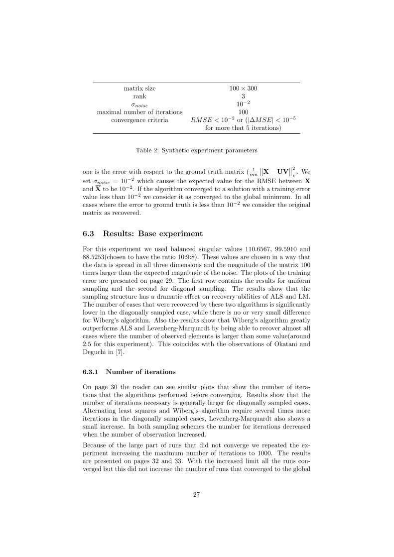
matrix size 100× 300rank 3σnoise 10−2

maximal number of iterations 100convergence criteria RMSE < 10−2 or (|∆MSE| < 10−5

for more that 5 iterations)

Table 2: Synthetic experiment parameters

one is the error with respect to the ground truth matrix ( 1mn

∥∥X−UV∥∥2

F. We

set σnoise = 10−2 which causes the expected value for the RMSE between Xand X to be 10−2. If the algorithm converged to a solution with a training errorvalue less than 10−2 we consider it as converged to the global minimum. In allcases where the error to ground truth is less than 10−2 we consider the originalmatrix as recovered.

6.3 Results: Base experiment

For this experiment we used balanced singular values 110.6567, 99.5910 and88.5253(chosen to have the ratio 10:9:8). These values are chosen in a way thatthe data is spread in all three dimensions and the magnitude of the matrix 100times larger than the expected magnitude of the noise. The plots of the trainingerror are presented on page 29. The first row contains the results for uniformsampling and the second for diagonal sampling. The results show that thesampling structure has a dramatic effect on recovery abilities of ALS and LM.The number of cases that were recovered by these two algorithms is significantlylower in the diagonally sampled case, while there is no or very small differencefor Wiberg’s algorithm. Also the results show that Wiberg’s algorithm greatlyoutperforms ALS and Levenberg-Marquardt by being able to recover almost allcases where the number of observed elements is larger than some value(around2.5 for this experiment). This coincides with the observations of Okatani andDeguchi in [7].

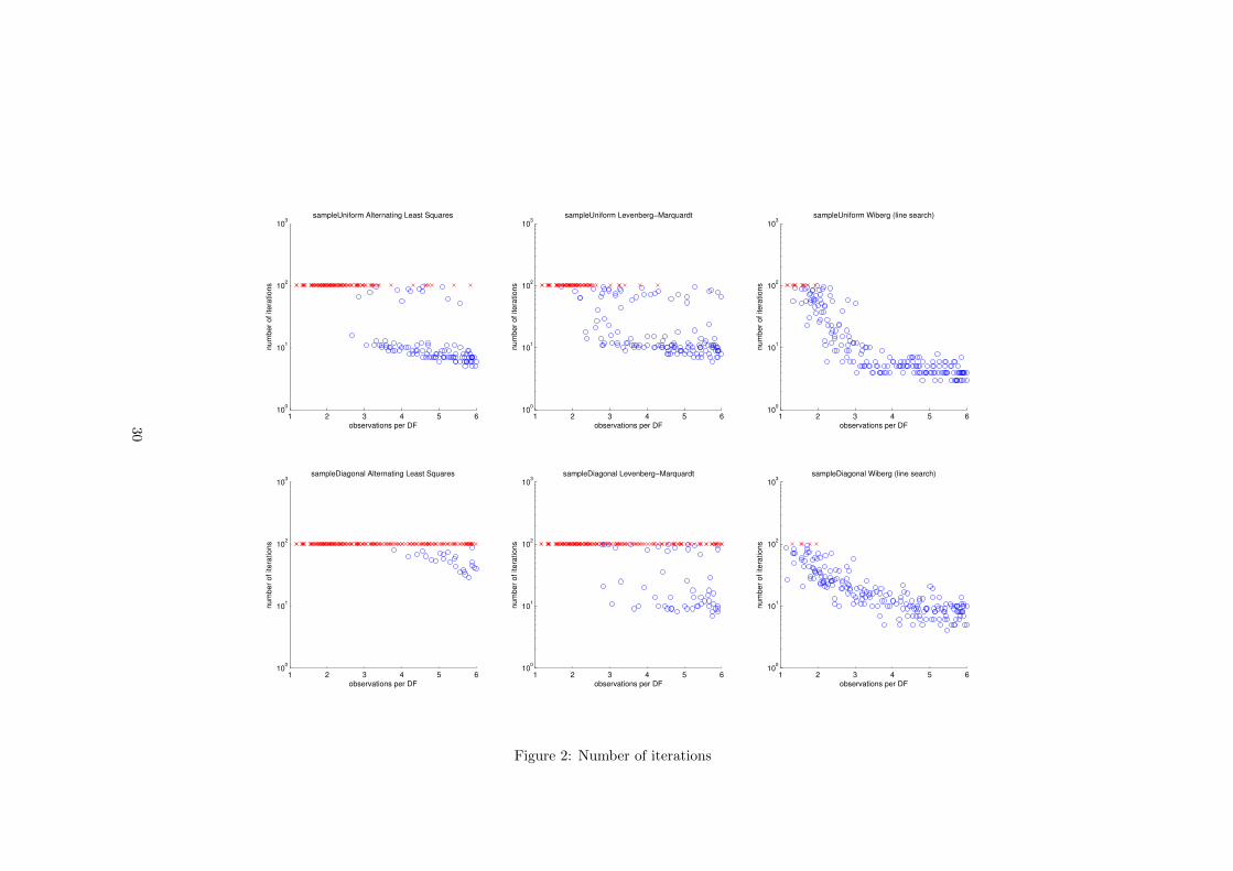
6.3.1 Number of iterations

On page 30 the reader can see similar plots that show the number of itera-tions that the algorithms performed before converging. Results show that thenumber of iterations necessary is generally larger for diagonally sampled cases.Alternating least squares and Wiberg’s algorithm require several times moreiterations in the diagonally sampled cases, Levenberg-Marquardt also shows asmall increase. In both sampling schemes the number for iterations decreasedwhen the number of observation increased.

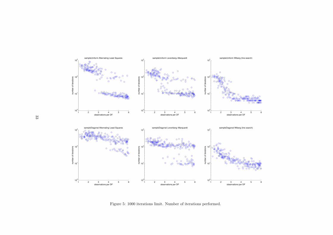
Because of the large part of runs that did not converge we repeated the ex-periment increasing the maximum number of iterations to 1000. The resultsare presented on pages 32 and 33. With the increased limit all the runs con-verged but this did not increase the number of runs that converged to the global

27

minimum. The behavior commonly observed during experiments was that de-pending on the starting point the algorithm either converged very fast to theglobal minimum or flat-lined for a long time before getting stuck at a local mini-mum. This caused the two distinct point clouds in the error and iteration plots.This experiment shows that in most cases these flat-lined cases are hopeless andit is reasonable to terminate the algorithm early if it does not converge in somenumber of iterations(i.e. 100). In such situations it is more likely to reach theglobal optimum by restarting the optimization from another random point.

6.3.2 Generalization error

On page 31 is presented the error to ground truth. It shows that solutionswhich correspond to a global minimum of the cost function generalize well andgeneralization error decreases as the number of observations increases. In somecases with low number of observations Wiberg’s algorithm converged to theglobal minimum of the cost function but the solution does not generalize wellto unseen data. This is visible in the plots as runs where the final value ofthe training error at the global minimum is lower than 10−2 but the error toground truth matrix is larger than 10−2. This is a problem of the used leastsquares model and nothing to do with the optimization procedure. In Sec. 7.5we propose a way to regularize structure-from-motion problems. Initially weexpected that this can counter overfitting but we could not observe this in ourexperiments.

28

1 2 3 4 5 610

−3

10−2

10−1

100

101

observations per DF

RM

SE

(tra

inin

g)

sampleUniform Alternating Least Squares

1 2 3 4 5 610

−3

10−2

10−1

100

101

observations per DF

RM

SE

(tra

inin

g)

sampleUniform Levenberg−Marquardt

1 2 3 4 5 610

−3

10−2

10−1

100

101

observations per DF

RM

SE

(tra

inin

g)

sampleUniform Wiberg (line search)

1 2 3 4 5 610

−3

10−2

10−1

100

101

observations per DF

RM

SE

(tra

inin

g)

sampleDiagonal Alternating Least Squares

1 2 3 4 5 610

−3

10−2

10−1

100

101

observations per DF

RM

SE

(tra

inin

g)

sampleDiagonal Levenberg−Marquardt

1 2 3 4 5 610

−3

10−2

10−1

100

101

observations per DF

RM

SE

(tra

inin

g)

sampleDiagonal Wiberg (line search)

Figure 1: Training error

29

1 2 3 4 5 610

0

101

102

103

observations per DF

nu

mb

er

of

ite

ratio

ns

sampleUniform Alternating Least Squares

1 2 3 4 5 610

0

101

102

103

observations per DF

nu

mb

er

of

ite

ratio

ns

sampleUniform Levenberg−Marquardt

1 2 3 4 5 610

0

101

102

103

observations per DF

nu

mb

er

of

ite

ratio

ns

sampleUniform Wiberg (line search)

1 2 3 4 5 610

0

101

102

103

observations per DF

nu

mb

er

of

ite

ratio

ns

sampleDiagonal Alternating Least Squares

1 2 3 4 5 610

0

101

102

103

observations per DF

nu

mb

er

of

ite

ratio

ns

sampleDiagonal Levenberg−Marquardt

1 2 3 4 5 610

0

101

102

103

observations per DF

nu

mb

er

of

ite

ratio

ns

sampleDiagonal Wiberg (line search)

Figure 2: Number of iterations

30

1 2 3 4 5 6

10−2

100

102

104

106

observations per DF

RM

SE

(to

gro

un

d t

ruth

)

sampleUniform Alternating Least Squares

1 2 3 4 5 6

10−2

100

102

104

106

observations per DF

RM

SE

(to

gro

un

d t

ruth

)

sampleUniform Levenberg−Marquardt

1 2 3 4 5 6

10−2

100

102

104

106

observations per DF

RM

SE

(to

gro

un

d t

ruth

)

sampleUniform Wiberg (line search)

1 2 3 4 5 6

10−2

100

102

104

106

observations per DF

RM

SE

(to

gro

un

d t

ruth

)

sampleDiagonal Alternating Least Squares

1 2 3 4 5 6

10−2

100

102

104

106

observations per DF

RM

SE

(to

gro

un

d t

ruth

)

sampleDiagonal Levenberg−Marquardt

1 2 3 4 5 6

10−2

100

102

104

106

observations per DF

RM

SE

(to

gro

un

d t

ruth

)

sampleDiagonal Wiberg (line search)

Figure 3: Error to ground truth

31

1 2 3 4 5 610

−3

10−2

10−1

100

101

observations per DF

RM

SE

(tra

inin

g)

sampleUniform Alternating Least Squares

1 2 3 4 5 610

−3

10−2

10−1

100

101

observations per DF

RM

SE

(tra

inin

g)

sampleUniform Levenberg−Marquardt

1 2 3 4 5 610

−3

10−2

10−1

100

101

observations per DF

RM

SE

(tra

inin

g)

sampleUniform Wiberg (line search)

1 2 3 4 5 610

−3

10−2

10−1

100

101

observations per DF

RM

SE

(tra

inin

g)

sampleDiagonal Alternating Least Squares

1 2 3 4 5 610

−3

10−2

10−1

100

101

observations per DF

RM

SE

(tra

inin

g)

sampleDiagonal Levenberg−Marquardt

1 2 3 4 5 610

−3

10−2

10−1

100

101

observations per DF

RM

SE

(tra

inin

g)

sampleDiagonal Wiberg (line search)

Figure 4: 1000 iterations limit. Training error.

32

1 2 3 4 5 610

0

101

102

103

observations per DF

nu

mb

er

of

ite

ratio

ns

sampleUniform Alternating Least Squares

1 2 3 4 5 610

0

101

102

103

observations per DF

nu

mb

er

of

ite

ratio

ns

sampleUniform Levenberg−Marquardt

1 2 3 4 5 610

0

101

102

103

observations per DF

nu

mb

er

of

ite

ratio

ns

sampleUniform Wiberg (line search)

1 2 3 4 5 610

0

101

102

103

observations per DF

nu

mb

er

of

ite

ratio

ns

sampleDiagonal Alternating Least Squares

1 2 3 4 5 610

0

101

102

103

observations per DF

nu

mb

er

of

ite

ratio

ns

sampleDiagonal Levenberg−Marquardt

1 2 3 4 5 610

0

101

102

103

observations per DF

nu

mb

er

of

ite

ratio

ns

sampleDiagonal Wiberg (line search)

Figure 5: 1000 iterations limit. Number of iterations performed.

33

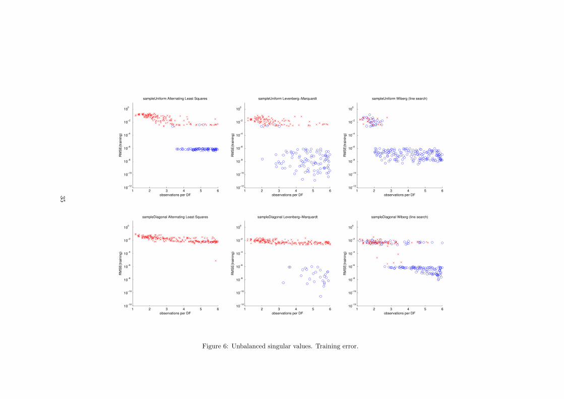
6.4 Unbalanced singular values

In real-world structure from motion problems, there are sometimes large dif-ferences in the magnitude of the singular values. For example in the dinosaurdataset without normalization the largest singular value is 5 to 10 times largerthan the rest. In order to study the effect of such dis-balance on the recoveryprocess we performed an experiment in which the largest non-zero singular val-ues have the ratio 100:10:1. In such situation the component that correspondsto the smallest singular value can be mistaken for noise. That is why no noisewas added. Because of that the global minimum has zero value of the costfunction and the threshold for stopping the optimization was reduced to 10−6.

The results are presented on page 35. They show that such dis-balance in thesingular values can reduce the recovery performance of all algorithms, especiallyin the diagonally sampled case. For all algorithms there were more runs thatconverged to local minima. ALS never converged on diagonally sampled cases.These results show that when applying matrix factorization to real-world datacare must be taken to normalize the input data in a way that will reduce thedifference between singular values.

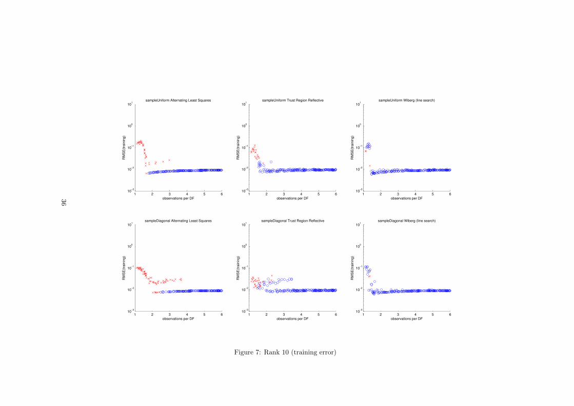
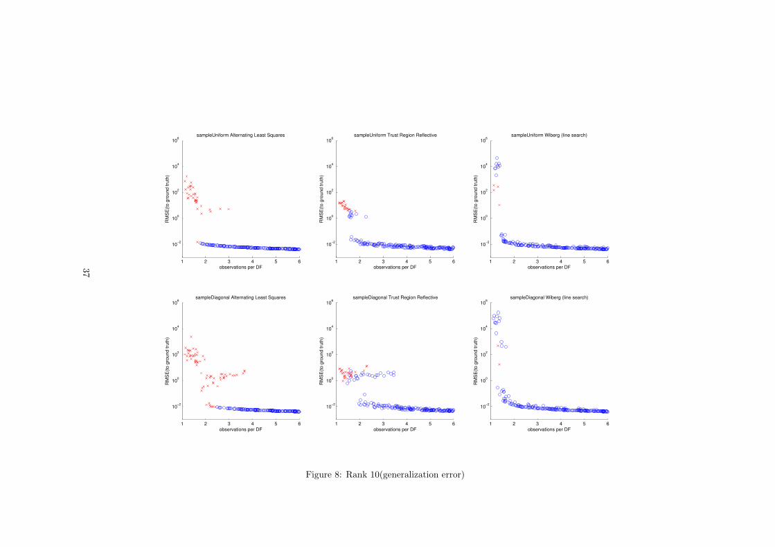
6.5 Large rank matrices

It was also interesting to see how the performance of the algorithms changeswhen the rank of the matrices increases. We performed an experiment in whichthe ground truth matrices are of rank 10 with singular values ratio 10:9:...:2:1.Because of the increased number of variables involved in the optimization, theLevenberg-Marquardt implementation in MATLAB ran out of memory andcould not complete the experiment. Instead we included the Trust-Region-Reflective algorithm that is available in MATLAB, which uses an iterativemethod to solve for the step direction and needs less memory. The resultsare presented on page 36(training error) and 37(generalization error). It is im-portant to note that in these plots the horizontal axis has a different scale dueto the increased number degrees of freedom of the model. In this experimentWiberg’s algorithm again outperformed ALS and LM. In all but a few runs itconverged to the global minimum. However in cases when the number of obser-vations is low such global minimum does not generalize well. ALS and LM alsoalways reach the global minimum for runs with more than roughly 4 observationper degree of freedom for the diagonally sampled case but this corresponds tosampling in a diagonal band that covers more than 75% of the matrix. In thiscase the diagonal structure is almost lost.

34

1 2 3 4 5 610

−12

10−10

10−8

10−6

10−4

10−2

100

observations per DF

RM

SE

(tra

inin

g)

sampleUniform Alternating Least Squares

1 2 3 4 5 610

−12

10−10

10−8

10−6

10−4

10−2

100

observations per DF

RM

SE

(tra

inin

g)

sampleUniform Levenberg−Marquardt

1 2 3 4 5 610

−12

10−10

10−8

10−6

10−4

10−2

100

observations per DF

RM

SE

(tra

inin

g)

sampleUniform Wiberg (line search)

1 2 3 4 5 610

−12

10−10

10−8

10−6

10−4

10−2

100

observations per DF

RM

SE

(tra

inin

g)

sampleDiagonal Alternating Least Squares

1 2 3 4 5 610

−12

10−10

10−8

10−6

10−4

10−2

100

observations per DF

RM

SE

(tra

inin

g)

sampleDiagonal Levenberg−Marquardt

1 2 3 4 5 610

−12

10−10

10−8

10−6

10−4

10−2

100

observations per DF

RM

SE

(tra

inin

g)

sampleDiagonal Wiberg (line search)

Figure 6: Unbalanced singular values. Training error.

35

1 2 3 4 5 610

−3

10−2

10−1

100

101

observations per DF

RM

SE

(tra

inin

g)

sampleUniform Alternating Least Squares

1 2 3 4 5 610

−3

10−2

10−1

100

101

observations per DF

RM

SE

(tra

inin

g)

sampleUniform Trust Region Reflective

1 2 3 4 5 610

−3

10−2

10−1

100

101

observations per DF

RM

SE

(tra

inin

g)

sampleUniform Wiberg (line search)

1 2 3 4 5 610

−3

10−2

10−1

100

101

observations per DF

RM

SE

(tra

inin

g)

sampleDiagonal Alternating Least Squares

1 2 3 4 5 610

−3

10−2

10−1

100

101

observations per DF

RM

SE

(tra

inin

g)

sampleDiagonal Trust Region Reflective

1 2 3 4 5 610

−3

10−2

10−1

100

101

observations per DF

RM

SE

(tra

inin

g)

sampleDiagonal Wiberg (line search)

Figure 7: Rank 10 (training error)

36

1 2 3 4 5 6

10−2

100

102

104

106

observations per DF

RM

SE

(to

gro

un

d t

ruth

)

sampleUniform Alternating Least Squares

1 2 3 4 5 6

10−2

100

102

104

106

observations per DF

RM

SE

(to

gro

un

d t

ruth

)

sampleUniform Trust Region Reflective

1 2 3 4 5 6

10−2

100

102

104

106

observations per DF

RM

SE

(to

gro

un

d t

ruth

)

sampleUniform Wiberg (line search)

1 2 3 4 5 6

10−2

100

102

104

106

observations per DF

RM

SE

(to

gro

un

d t

ruth

)

sampleDiagonal Alternating Least Squares

1 2 3 4 5 6

10−2

100

102

104

106

observations per DF

RM

SE

(to

gro

un

d t

ruth

)

sampleDiagonal Trust Region Reflective

1 2 3 4 5 6

10−2

100

102

104

106

observations per DF

RM

SE

(to

gro

un

d t

ruth

)

sampleDiagonal Wiberg (line search)

Figure 8: Rank 10(generalization error)

37

7 Application to Affine Structure from Motionproblems

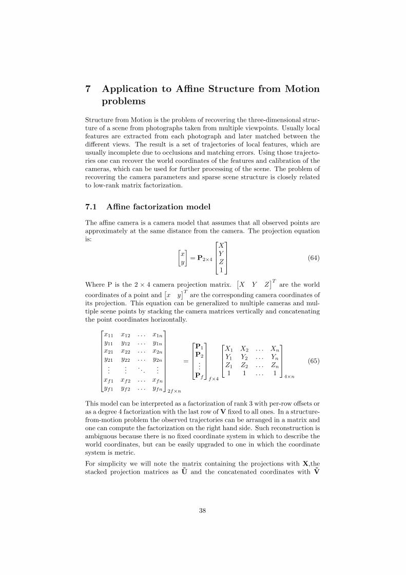
Structure from Motion is the problem of recovering the three-dimensional struc-ture of a scene from photographs taken from multiple viewpoints. Usually localfeatures are extracted from each photograph and later matched between thedifferent views. The result is a set of trajectories of local features, which areusually incomplete due to occlusions and matching errors. Using those trajecto-ries one can recover the world coordinates of the features and calibration of thecameras, which can be used for further processing of the scene. The problem ofrecovering the camera parameters and sparse scene structure is closely relatedto low-rank matrix factorization.

7.1 Affine factorization model

The affine camera is a camera model that assumes that all observed points areapproximately at the same distance from the camera. The projection equationis: [

xy

]= P2×4

XYZ1

(64)

Where P is the 2 × 4 camera projection matrix.[X Y Z

]Tare the world

coordinates of a point and[x y

]Tare the corresponding camera coordinates of

its projection. This equation can be generalized to multiple cameras and mul-tiple scene points by stacking the camera matrices vertically and concatenatingthe point coordinates horizontally.

x11 x12 . . . x1n

y11 y12 . . . y1n

x21 x22 . . . x2n

y21 y22 . . . y2n

......

. . ....

xf1 xf2 . . . xfnyf1 yf2 . . . yfn

2f×n

=

P1

P2

...Pf

f×4

X1 X2 . . . Xn

Y1 Y2 . . . YnZ1 Z2 . . . Zn1 1 . . . 1

4×n

(65)

This model can be interpreted as a factorization of rank 3 with per-row offsets oras a degree 4 factorization with the last row of V fixed to all ones. In a structure-from-motion problem the observed trajectories can be arranged in a matrix andone can compute the factorization on the right hand side. Such reconstruction isambiguous because there is no fixed coordinate system in which to describe theworld coordinates, but can be easily upgraded to one in which the coordinatesystem is metric.

For simplicity we will note the matrix containing the projections with X,thestacked projection matrices as U and the concatenated coordinates with V

38

similar to the low-rank factorization model. They can be decomposed as:

U =[U z

]V =

[V

1T

](66)

U and V are components of a 3-dimensional low-rank factorization and z arethe per-row offsets. The model can be written as:

X = UV =[U z

] [V

1T

]= UV + z1

T(67)

This model can be vectorized similar to the low-rank factorization model:

x = S vec [X] = Fu = Gv + w

where

F = S(VT ⊗ Im)

G = S(In ⊗U)

u = vec[U]

v = vec [V]

w = S vec[z1

T]

(68)

F and G are the Jacobians of the model with respect to u and v. w is a vector ofper-data point offsets that are derived from z. Similarly to the general low-rankfactorization, this model is bilinear. This means that one can formulate theleast squares cost function and fit the model to data using the same algorithms.ALS, LM and Wibergs’s algorithm can be adapted operate on affine structure-from-motion data. The complexity of the algorithms does not change. Alsothe experiments on synthetic data presented in Sec. 8 show that they also havesimilar properties to their non-affine variants.

7.2 Alternating least squares.

ALS is trivial to modify to include the per-camera offsets. The procedure be-comes alternation between optimizing U, which consists of U and the offsets z,and optimizing V. The offsets have to be subtracted when optimizing V.

39

Algorithm 7 Alternating Least Squares: affine camera version

1: Initialize U and V.2: repeat

3: V←[

V

1T

]4: for i = 1 to m do5: mask ← indexes of observed elements in the i-th row of X6: ui: ← lsqlin(VT

:,mask , XT

i,mask)7: end for8: U← U1:3,4

9: z← U:,4

10: for j = 1 to n do11: mask ← indexes of observed elements in the j-th column of X12: v:j ← lsqlin(Umask,: , Xmask,j − zmask)13: end for14: until converged

7.3 Gauss-Newton based methods.

In order to adapt GN-based algorithms one has to compute the Jacobian of theresidual with respect to the parameters. If the problem is parametrized with

the vector

[uv

]the Jacobian is:

∂r

∂

[uv

] =[∂r∂u

∂r∂v

]=[∂(Fu−x)

∂u

∂(Gv+S vec[z1T ]−x)

∂v

]=[F G

](69)

7.4 Wiberg’s algorithm.

Wiberg’s algorithms is derived in the same way as the version without offsets.The formulas for the residual and the approximate Jacobian are:

r = QG(x−w) J ≈ QGF (70)

Where G is again block-diagonal and can be easily orthogonalized. The algo-rithm was implemented using the LSQR algorithm to compute the step directionin the same way as the non-affine variant.

7.5 Orthogonality constraints

An affine camera matrix can be decomposed in the following way:

P =

[uT1 z1

uT2 z2

](71)

where uT1 and uT2 are vectors that define the axes of the camera projection planeand (z1, z2) is an offset in this plane. Real-world cameras have axes that are ap-proximately orthogonal and uniformly scaled. The factorization representation

40

is over-parametrized because it allows cameras that have non-uniformly scaledand non-orthogonal axes. To counter this, soft constraints were added to thecost function in the form of additional residuals which should be minimized inleast squares sense. This augmented cost function minimization is again a least-squares problem and can be minimized using Gauss-Newton style methods. Asthe reader will be able to see in next section, this caused Wiberg’s algorithm toreach the global minimum more often and in less iterations.

The residual with orthogonality constraints is defined as:

r =

√ 1l rm√λm rc

rm = QG(x−w) (model residual)

rc =

uT1 u2 − 0uT1 u1 − 1uT2 u2 − 1uT3 u4 − 0uT3 u3 − 1uT4 u4 − 1

...uTm−1um − 0

uTm−1um−1 − 1uTmum − 1

(orthogonality constraints residual)

(72)

There are two sets of residuals that are involved. First rm that corresponds tohow well the model matches the data. It is weighted by 1√

lin order to make the

value independent of the number of residuals. The second set rc correspondsto the orthogonality and scale constraints for the camera projection matrices.There are 3 constraints per camera. If they are matched exactly then thenthe camera has orthogonal and uniformly scaled axes. The constraint residuals

are scaled by√

λm . This ensures that the value of the error function will be

independent of the number of cameras. λ is a hyper-parameter that controls thetrade-off between fitting of the model and fitting the orthogonality constraints.The corresponding least-squares cost function is:

E(U,V) =1

l

∥∥rm∥∥2

2+λ

m

∥∥rc∥∥2

2

=1

l

∥∥∥∥M� (U

[V

1T

]−X

)∥∥∥∥F

+λ

m

m2∑i=1

((uT2i−1u2i)2 + (uT2i−1u2i−1 − 1)2 + (uT2iu2i − 1)2)

(73)

This cost function can be re-parametrized as a function of U only in the spiritof Wiberg’s algorithm. When U is fixed the value of the rc is also fixed and theoptimal value for V is the same as in the non-constrained case. The Jacobian

41

can be split in two parts that correspond to the model and to the constraints.

J =

[JmJc

]=

√ 1l∂ρm

∂u√λm∂ρc

∂u

(74)

Where ρm and ρc are the two parts of the residual as function of u only similarto the derivation of Wiberg’s algorithm. The first part is the same of the non-regularizes version multiplied by 1√

l:

∂ρm∂u≈ QGF (75)

In the second part each row of U influences only the three residuals that cor-respond to the same camera. The Jacobian is constructed using the followingequations for each camera, setting all other elements to zero and multiplying by√

λm .

∂ρi,1c∂u2i−1

= u2i

∂ρi,1c∂u2i

= u2i−1

∂ρi,2c∂u2i−1

= 2u2i−1

∂ρi,3c∂u2i

= 2u2i

(76)

Knowing the Jacobian, Gauss-Newton steps are performed in a way similarto the standard Wiberg algorithm. Step direction is solved using the LSQRmethod. Multiplication by the Jacobian is performed by splitting it into multi-plication by the two parts of the Jacobian:

Jy =

[JmJc

]y =

[JmyJcy

]=

√ 1l∂ρm

∂u y√λm∂ρc

∂u y

=

√ 1lQGFy√λm∂ρc

∂u y

(77)

Multiplication by QG is done using an orthogonalized version of G. ∂ρc

∂u hasO(m) non zero elements and does not increase the complexity of the algorithm.Furthermore the experiments show that adding the orthogonality constraintscan cause Wiberg’s algorithm to converge in less iterations.

7.6 Normalization

The experiments on synthetic data showed that unbalanced singular values candecrease the chances of all algorithms to converge to the global minimum. Tocounter this we normalized the data. Points in each camera are first centered totheir mean. After that the points observed by all cameras together are scaled ina way such that their standard deviation becomes one. The scaling is isotropicin in the x- and y-direction and the same scaling factor is used for all cameras.

42

This way minimizing the least-squares error on the normalized data is equivalentto minimizing it on the original dataset. For example on the dinosaur dataset,that we used for real-world data tests, this changes the ratio of the singularvalues of the recovered model from approximately 100:19:15:7 to approximately100:63:32:28.

43

8 Experiments on Structure-from-Motion Data

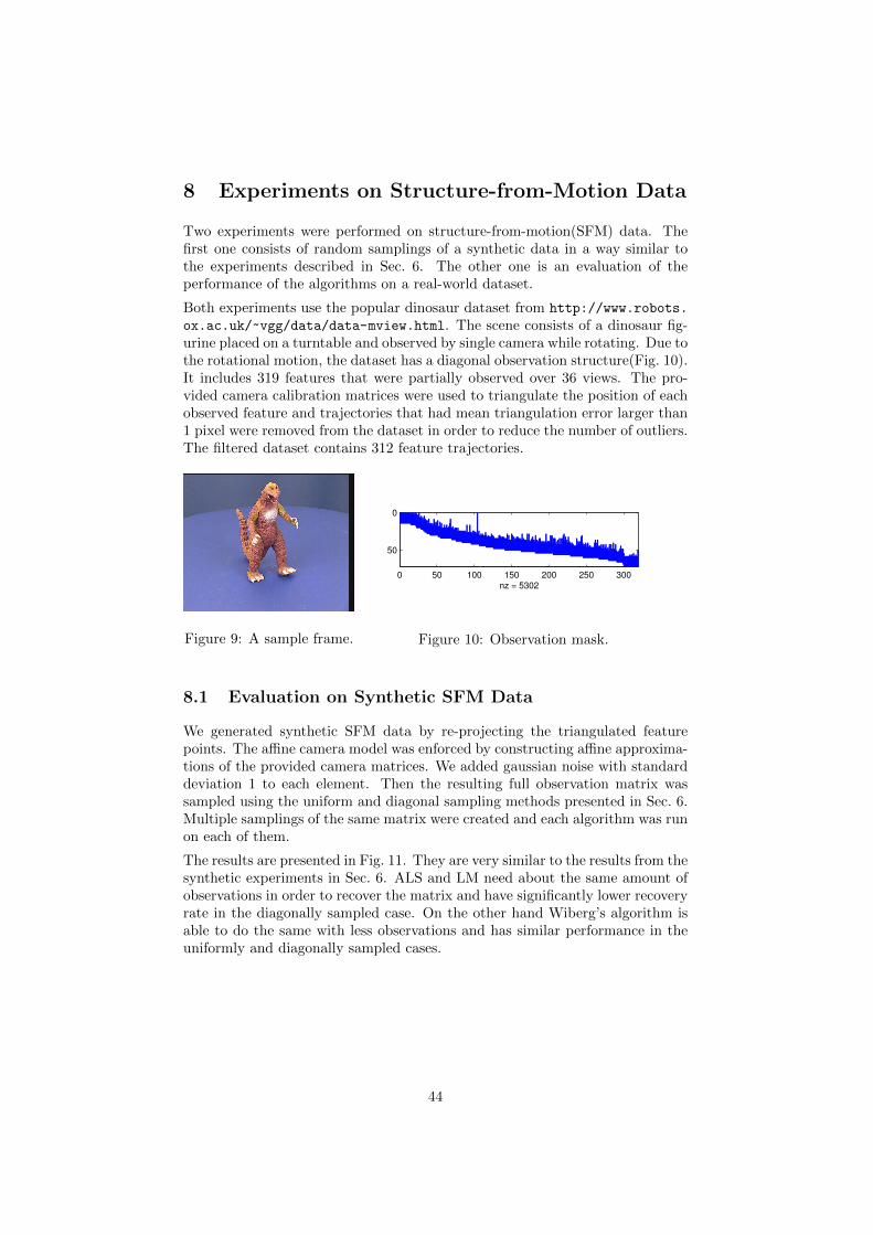
Two experiments were performed on structure-from-motion(SFM) data. Thefirst one consists of random samplings of a synthetic data in a way similar tothe experiments described in Sec. 6. The other one is an evaluation of theperformance of the algorithms on a real-world dataset.

Both experiments use the popular dinosaur dataset from http://www.robots.

ox.ac.uk/~vgg/data/data-mview.html. The scene consists of a dinosaur fig-urine placed on a turntable and observed by single camera while rotating. Due tothe rotational motion, the dataset has a diagonal observation structure(Fig. 10).It includes 319 features that were partially observed over 36 views. The pro-vided camera calibration matrices were used to triangulate the position of eachobserved feature and trajectories that had mean triangulation error larger than1 pixel were removed from the dataset in order to reduce the number of outliers.The filtered dataset contains 312 feature trajectories.

Figure 9: A sample frame.

0 50 100 150 200 250 300

0

50

nz = 5302

Figure 10: Observation mask.

8.1 Evaluation on Synthetic SFM Data

We generated synthetic SFM data by re-projecting the triangulated featurepoints. The affine camera model was enforced by constructing affine approxima-tions of the provided camera matrices. We added gaussian noise with standarddeviation 1 to each element. Then the resulting full observation matrix wassampled using the uniform and diagonal sampling methods presented in Sec. 6.Multiple samplings of the same matrix were created and each algorithm was runon each of them.

The results are presented in Fig. 11. They are very similar to the results from thesynthetic experiments in Sec. 6. ALS and LM need about the same amount ofobservations in order to recover the matrix and have significantly lower recoveryrate in the diagonally sampled case. On the other hand Wiberg’s algorithm isable to do the same with less observations and has similar performance in theuniformly and diagonally sampled cases.

44

1 2 3 4 5 610

−1

100

101

102

observations per DF

RM

SE

(tra

inin

g)

uniform sampling / ALS

1 2 3 4 5 610

−1

100

101

102

observations per DF

RM

SE

(tra

inin

g)

diagonal sampling / ALS

1 2 3 4 5 610

−1

100

101

102

observations per DF

RM

SE

(tra

inin

g)

uniform sampling / LM

1 2 3 4 5 610

−1

100

101

102

observations per DF

RM

SE

(tra

inin

g)

diagonal sampling / LM

1 2 3 4 5 610

−1

100

101

102

observations per DF

RM

SE

(tra

inin

g)

uniform sampling / Wiberg

1 2 3 4 5 610

−1

100

101

102

observations per DF

RM

SE

(tra

inin

g)

diagonal sampling / Wiberg

Figure 11: Results for synthetic affine structure-from-motion data. Training error.

45

8.2 Evaluation on Real-World SFM Data

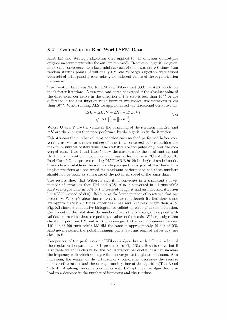
ALS, LM and Wiberg’s algorithm were applied to the dinosaur dataset(theoriginal measurements with the outliers removed). Because all algorithms guar-antee only convergence to a local minima, each of them was ran 200 times fromrandom starting points. Additionally LM and Wiberg’s algorithm were testedwith added orthogonality constraints, for different values of the regularizationparameter λ.

The iteration limit was 300 for LM and Wiberg and 3000 for ALS which hasmuch faster iterations. A run was considered converged if the absolute value ofthe directional derivative in the direction of the step is less than 10−8 or thedifference in the cost function value between two consecutive iterations is lessthan 10−8. When running ALS we approximated the directional derivative as:

E(U + ∆U,V + ∆V)− E(U,V)√∥∥∆U∥∥2

F+∥∥∆V

∥∥2

F

(78)

Where U and V are the values in the beginning of the iteration and ∆U and∆V are the changes that were performed by the algorithm in the iteration.

Tab. 3 shows the number of iterations that each method performed before con-verging as well as the percentage of runs that converged before reaching themaximum number of iterations. The statistics are computed only over the con-verged runs. Tab. 4 and Tab. 5 show the statistics for the total runtime andthe time per iteration. The experiment was performed on a PC with 2.66GHzIntel Core 2 Quad processor using MATLAB R2010b in single threaded mode.The code is available in the source code package that is part of this thesis. Theimplementations are not tuned for maximum performance and these numbersshould not be taken as a measure of the potential speed of the algorithms.

The results show that Wiberg’s algorithm converges in a significantly lowernumber of iterations than LM and ALS. Also it converged in all runs whileALS converged only in 60% of the cases although it had an increased iterationlimit(3000 instead of 300). Because of the lower number of iterations that arenecessary, Wiberg’s algorithm converges faster, although its iterations timesare approximately 2.5 times longer than LM and 30 times longer than ALS.Fig. 8.2 shows a cumulative histogram of validation error of the final solution.Each point on this plot show the number of runs that converged to a point withvalidation error less than or equal to the value on the x-axis. Wiberg’s algorithmclearly outperforms LM and ALS. It converged to the global minimum in over140 out of 200 runs, while LM did the same in approximately 20 out of 200.ALS never reached the global minimum but a few runs reached values that areclose to it.

Comparison of the performance of Wiberg’s algorithm with different values ofthe regularization parameter λ is presented in Fig. 13(a). Results show that ifa suitable weight is chosen for the regularization parameter, this can increasethe frequency with which the algorithm converges to the global minimum. Alsoincreasing the weight of the orthogonality constraints decreases the averagenumber of iterations and the average running time of the algorithm(Tab. 3 andTab. 4). Applying the same constraints with LM optimization algorithm, alsolead to a decrease in the number of iterations and the runtime.

46

λ mean median min max converged

ALS 0 1522.57 1503 96 2973 60.5%LM 0 166.362 180 11 299 92.5%LM 1e-05 144.396 149 11 299 98.5%LM 0.0001 137.75 145 11 287 98%LM 0.001 131.434 132.5 11 300 98%Wiberg 0 44.315 33 10 180 100%Wiberg 1e-05 46.095 38 11 216 100%Wiberg 0.0001 36.575 30 10 146 100%Winerg 0.001 32 25.5 9 221 100%

Table 3: Number of iterations until convergence.

λ mean median min max

ALS 0 24.3761 28.7625 1.06374 36.8557LM 0 22.5693 23.7509 0.815505 39.388LM 1e-05 20.8813 21.5632 0.90971 43.467LM 0.0001 20.0494 20.9168 0.911515 44.3537LM 0.001 19.1811 19.4056 0.907933 44.3353Wiberg 0 14.7841 11.0878 3.02743 60.5895Wiberg 1e-05 15.3595 12.7793 3.38493 69.279Wiberg 0.0001 12.1494 9.78592 3.04298 47.7387Winerg 0.001 10.6074 8.28384 2.69137 72.5056

Table 4: Running time (seconds).

λ mean median min max

ALS 0 0.0115673 0.0115539 0.0110785 0.0123617LM 0 0.124534 0.127875 0.0741368 0.13105LM 1e-05 0.140217 0.142091 0.0827009 0.146441LM 0.0001 0.138568 0.141998 0.082865 0.148231LM 0.001 0.137839 0.142162 0.0814647 0.151932Wiberg 0 0.329286 0.329186 0.302743 0.363601Wiberg 1e-05 0.331168 0.332082 0.307721 0.361889Wiberg 0.0001 0.32942 0.329366 0.304298 0.357182Winerg 0.001 0.327501 0.327457 0.299041 0.368501

Table 5: Time per iteration (seconds).

47

10−1

100

101

0

20

40

60

80

100

120

140

160

180

200

Validation error (pixels)

Cum

ula

tive n

um

ber

of ru

ns

ALS

LM

Wiberg

Figure 12: Comparison of SFM algorithms on real-world data.

48

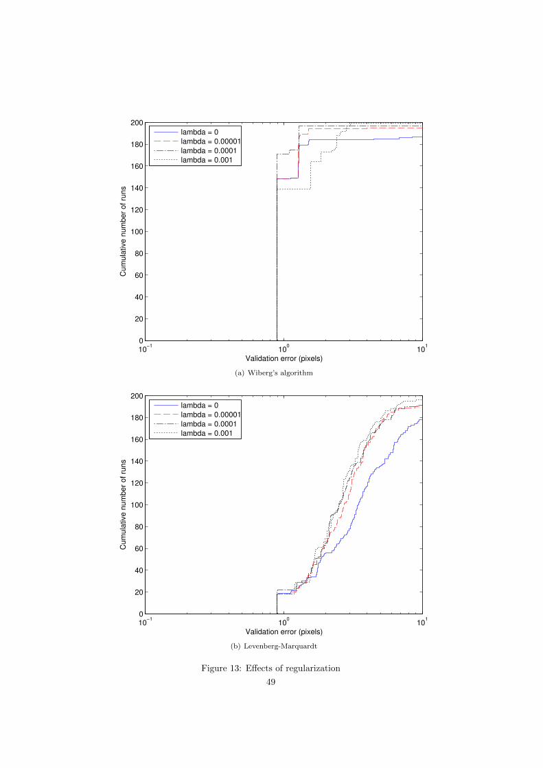
10−1

100

101

0

20

40

60

80

100

120

140

160

180

200

Validation error (pixels)

Cum

ula

tive n

um

ber

of ru

ns

lambda = 0

lambda = 0.00001

lambda = 0.0001

lambda = 0.001

(a) Wiberg’s algorithm

10−1

100

101

0

20

40

60

80

100

120

140

160

180

200

Validation error (pixels)

Cum

ula

tive n

um

ber

of ru

ns

lambda = 0

lambda = 0.00001

lambda = 0.0001

lambda = 0.001

(b) Levenberg-Marquardt

Figure 13: Effects of regularization

49

9 Conclusion

In this thesis we compared several popular algorithms for low-rank matrix fac-torization with missing data. The comparison was performed on synthetic low-rank matrices, synthetic and real-world structure-from-motion data. Resultsshowed that Wiberg’s algorithm is able to solve problems with lower number ofobserved elements than the the ones that can be solved by applying Levenberg-Marquardt or Alternating Least Squares. Also WA converges more often to theglobal minimum and in significantly less iterations than LM or ALS.

We improved Wiberg’s algorithm in two important ways. First, we demon-strated how the sparsity and the algebraic properties of the problem can beused to obtain a more efficient implementation. The per-iteration computationalcomplexity of such implementation is similar to the most efficient implementa-tions of generic non-linear least squares methods like Levenberg-Marquardt,when they are applied to the low-rank factorization problem. Experimentsshowed these advantages can be observed in practice as a reduction in the con-vergence times and the number of runs that get stuck in a local minimum.Another improvement that we suggested is the addition of camera orthogonal-ity constraints in a way that does not change the least-squares form of the costfunction. Our results show that such constraints can further improve the con-vergence speed of WA and decrease the number of runs which get stuck in alocal minimum.

These improvements make Wiberg’s algorithm practical to use on large problemsand we believe it should be preferred over LM and ALS when solving low-rankmatrix factorization or affine SFM problems. One exception are problems inwhich very large fraction of the matrix elements is observed. There ALS has aspeed advantage due to its low iteration times. Because of the iterative natureof WA and ALS it is possible to combine the two algorithms in a way similar tothe hybrid methods that Buchanan described in [1]. This can possibly result ina method that is fast on matrices with few missing elements but is also able torecover matrices with many missing entries. Another interesting path for futurework is to explore the interactions between Wiberg’s algorithm outer iterationsand the LSQR inner iterations. For example a way to dynamically control thestopping conditions of the inner iterations for different outer iterations mayincrease the speed of the algorithm by calculating the step direction with lowerprecision when that will be sufficient for the outer iteration.

50

References

[1] A. M. Buchanan and A. W. Fitzgibbon. Damped newton algorithms formatrix factorization with missing data. 2005.

[2] A. Eriksson and A. Hengel. Efficient computation of robust low-rank matrixapproximations in the presence of missing data using the l1 norm, 2010.

[3] G. Golub and V. Pereyra. Separable nonlinear least squares: the variableprojection method and its applications. 2002.

[4] M. Hanke. On lanczos based methods for the regularization of discreteill-posed problems. 2001.

[5] R. Hartley and F. Schaffalitzky. Powerfactorization: 3d reconstruction withmissing or uncertain data, 2003.

[6] H.B. Nielsen K. Madsen and O. Tingleff. Methods for non-linear leastsquares problems, 2004.

[7] T. Okatani and K. Deguchi. On the wiberg algorithm for matrix factoriza-tion in the presence of missing components. 2006.

[8] C. Poelman and T. Kanade. A paraperspective factorization method forshape and motion recovery. Technical report, 1993.

[9] R. Salakhutdinov and A. Mnih. Bayesian probabilistic matrix factorizationusing markov chain monte carlo. 2008.

[10] P. Sturm and B. Triggs. A factorization based algorithm for multi-imageprojective structure and motion, 1996.

[11] C. Tomasi. Shape and motion from image streams under orthography: afactorization method. 1992.

51