in cell investigator in cell developer toolbox v1...in cell developer toolbox v1.9 user manual...
TRANSCRIPT

GE Healthcare
User Manual Supplement
IN Cell Investigator IN Cell Developer Toolbox v1.9
High-content image analysis software

1 Introduction1.1 Additions to the V1.7 release included: .................................................. 51.2 Additions to the V1.8 release include: ..................................................... 61.3 Additions to the V1.9 release include: ..................................................... 6
2 Image Transformation Protocols2.1 Extended Focus Transformation (v 1.8) .................................................. 72.1.1 Setting the Extended Focus Parameters..................................................... 82.2 Image Stitching (v 1.8) ..................................................................................112.2.1 Creating a Stitched Image.............................................................................. 112.3 Phase Contrast & DIC (v 1.9) ......................................................................18
3 Pre-processing Operations3.1 Pseudo Florescence Preprocessing (v 1.7) ..........................................233.2 Texture Transformation (v 1.8) .................................................................263.3 Shading Removal QSM (v 1.9) ...................................................................29
4 Segmentation Operations4.1 Version 1.7 Updates - Additional Parameters ...................................334.1.1 Intensity Segmentation Panel....................................................................... 334.1.2 Vesicle Segmentation Panel (v 1.7) ............................................................. 344.1.3 Nuclear Segmentation Panel ........................................................................ 354.1.4 Cytoplasm Segmentation Panel .................................................................. 364.2 Version 1.8 Updates ......................................................................................364.2.1 Shape Sensitive Segmentation within Vesicle Segmentation......... 364.3 Version 1.9 Updates ......................................................................................384.3.1 DT Watershed Segmentation........................................................................ 38
5 Post-processing Operations5.1 Watershed Clump Breaking (v 1.8) .........................................................415.1.1 Image Types and Processing ........................................................................ 445.2 Fill Holes (v 1.8) .................................................................................................455.3 Border Object Removal (v 1.8) ..................................................................465.3.1 Border Object Removal Combinations ................................................... 48
6 Classifiers in Developer Toolbox (v 1.7)6.1 Classification using a Threshold filter ...................................................506.2 Classification using a Linear Discriminant Filter ..............................546.3 Classification Using a Decision Tree Filter ..........................................59
7 Cell Tracking in Developer Toolbox (v 1.7)7.1 Overview .............................................................................................................637.2 Cell Tracking Dialog .......................................................................................637.2.1 Setting Cell Tracking Parameters................................................................ 647.2.2 Setting the Tracking Method (updated v1.8) .......................................... 677.3 Labels and Linked Track IDs ......................................................................697.4 Cell Tracking Data Output ..........................................................................71
IN Cell Developer Toolbox V1.9 User Manual 28-9274-22UM AB 3

7.5 Visualizing Results with Spotfire DecisionSite .................................. 72
8 Data Output8.1 Updates in v1.8/1.9 ....................................................................................... 778.2 Group Summary Table ................................................................................ 788.2.1 Data tab.................................................................................................................. 788.2.2 Definition tab ........................................................................................................ 798.2.3 Summary tab........................................................................................................ 818.2.4 File Menu Options............................................................................................... 818.2.5 Summary Tab Edit Menu................................................................................. 828.2.6 Connect to Spotfire DecisionSite.................................................................. 838.2.7 Save Group Summary with Protocol ......................................................... 83
9 Outline Display Options (v 1.7)
10 Context Modules10.1 Version 1.7 Updates ...................................................................................... 8710.2 Version 1.8 Updates ...................................................................................... 8910.2.1 Angiogenesis ........................................................................................................ 8910.3 Version 1.9 Updates ...................................................................................... 9010.3.1 Early Endosomal Markers ............................................................................... 9110.3.2 Neurite Outgrowth............................................................................................. 92
11 Additional Features11.1 Version 1.7 Enhancements ........................................................................ 9711.1.1 Multi-processor Support.................................................................................. 9711.1.2 Memory Management Improvements & New File Format............... 9811.1.3 Navigating Data Tables ................................................................................... 9911.2 Version 1.8 Enhancements ..................................................................... 10111.2.1 Plug-in Interface............................................................................................... 10111.2.1.1 Load plugins .....................................................................................................10211.2.1.2 Configure plug-ins ..........................................................................................10311.2.1.3 Configure plug-in directory ........................................................................10511.3 Version 1.9 Enhancements ..................................................................... 10511.3.1 Analyzing Image Stacks Other than IN Cell Analyzer
1000/2000.......................................................................................................... 10511.3.2 Interfacing with IN Cell Miner HCM ......................................................... 10711.3.2.1. Exporting Analysis Data To IN Cell Miner .............................................10711.3.2.2. Importing Analysis Data From IN Cell Miner........................................ 110
12 Rehosting your E-License
4 IN Cell Developer Toolbox V1.9 User Manual 28-9274-22UM AB

Introduction 1Additions to the V1.7 release included: 1.1
1 Introduction
This revision to the supplement to the IN Cell Developer Toolbox V1.6 High-content image analysis software User's Reference Manual, part number 28-4088-71, includes those features and functionalities available in IN Cell Developer Toolbox V1.7, as well as those new to IN Cell Developer Toolbox V1.8.
For a description of the user interface and the general features, please refer to the complete IN Cell Developer Toolbox 1.6 User Reference Manual.
1.1 Additions to the V1.7 release included:• Data Table Navigation - the LG3 analysis file type has been added to
Investigator 1.3 to deal more effectively with large image stacks.
• Cell Tracking - enables automated quantification of cell position, speed and direction as a function of time.
• Full integration of all 'canned' assays - analyze an image stack using one of the 'canned' modules including the new Multi-target Analysis module
• Classifiers - provide flexible tools for classification of objects in the image into multiple sub-populations.
• Group Summary Tables- analysis data can aggregated using user defined criteria, .e.g. to provide sub-population summaries
• New Context Module - a new context module, Cell Viability, has been added.
• In addition, updates were made to the existing context modules.
• New Preprocessing parameters in Pseudo Fluorescence - new preprocessing parameters can be applied to an image stack with transmitted light images prior to segmentation of a given target set.
• New Segmentation Parameters - new parameters were added to Intensity, Vesicle, Nuclear, and Cytoplasm segmentation.
• Outline Display Options - target labels and target outlines can be displayed on your images.
• Multi-processor support - provides increased computing power by using
IN Cell Developer Toolbox V1.9 User Manual 28-9274-22UM AB 5
1 Introduction1.2 Additions to the V1.8 release include:
advantages of multi-core and multi-CPU systems.
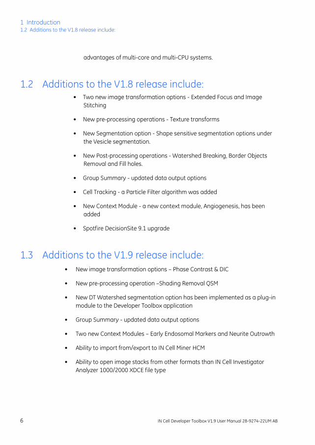
1.2 Additions to the V1.8 release include:• Two new image transformation options - Extended Focus and Image
Stitching
• New pre-processing operations - Texture transforms
• New Segmentation option - Shape sensitive segmentation options under the Vesicle segmentation.
• New Post-processing operations - Watershed Breaking, Border Objects Removal and Fill holes.
• Group Summary - updated data output options
• Cell Tracking - a Particle Filter algorithm was added
• New Context Module - a new context module, Angiogenesis, has been added
• Spotfire DecisionSite 9.1 upgrade
1.3 Additions to the V1.9 release include:• New image transformation options – Phase Contrast & DIC
• New pre-processing operation –Shading Removal QSM
• New DT Watershed segmentation option has been implemented as a plug-in module to the Developer Toolbox application
• Group Summary - updated data output options
• Two new Context Modules – Early Endosomal Markers and Neurite Outrowth
• Ability to import from/export to IN Cell Miner HCM
• Ability to open image stacks from other formats than IN Cell Investigator Analyzer 1000/2000 XDCE file type
6 IN Cell Developer Toolbox V1.9 User Manual 28-9274-22UM AB
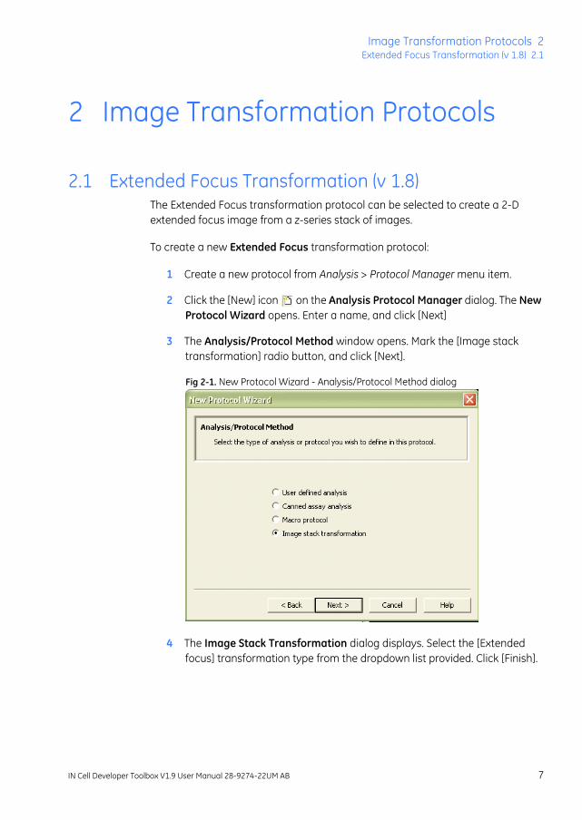
Image Transformation Protocols 2Extended Focus Transformation (v 1.8) 2.1
2 Image Transformation Protocols
2.1 Extended Focus Transformation (v 1.8) The Extended Focus transformation protocol can be selected to create a 2-D extended focus image from a z-series stack of images.
To create a new Extended Focus transformation protocol:
1 Create a new protocol from Analysis > Protocol Manager menu item.
2 Click the [New] icon on the Analysis Protocol Manager dialog. The New Protocol Wizard opens. Enter a name, and click [Next]
3 The Analysis/Protocol Method window opens. Mark the [Image stack transformation] radio button, and click [Next].
Fig 2-1. New Protocol Wizard - Analysis/Protocol Method dialog
4 The Image Stack Transformation dialog displays. Select the [Extended focus] transformation type from the dropdown list provided. Click [Finish].
IN Cell Developer Toolbox V1.9 User Manual 28-9274-22UM AB 7

2 Image Transformation Protocols2.1 Extended Focus Transformation (v 1.8)
Fig 2-2. New Protocol Wizard - Image Stack Transformation dialog
5 Select an image stack to transform using the View / Analyze Image Stack option on the Operations bar
2.1.1 Setting the Extended Focus Parameters The definition and editing of the extended focus transformation parameters is done in the Extended Focus Component Overview panel.
1 The Extended Focus Component Overview panel will open upon exiting the Wizard. You may modify any of the parameters as described in the table below.
8 IN Cell Developer Toolbox V1.9 User Manual 28-9274-22UM AB

Image Transformation Protocols 2Extended Focus Transformation (v 1.8) 2.1
Fig 2-3. Extended Focus parameters panel
Parameter Description
Mask size The size of the neighborhood surrounding a pixel used to estimate the focus measure. A minimal size of the objects of interest can serve as in the setting up the Mask size. Click on the Value to open the field for editing. Mask size is measured in pixels.
Power Parameter that controls contribution of pixels to the result of combination A value of 1 sets weight to be just proportional to focus measure Click on the Value to open the field for editing.
Focus measure type
Focus measure is a function with its maximum when pixel is in focus. Click on the Value field to open the dropdown list to select a focus measure:
• Variance
• Square of gradient
IN Cell Developer Toolbox V1.9 User Manual 28-9274-22UM AB 9

2 Image Transformation Protocols2.1 Extended Focus Transformation (v 1.8)
2 The Extended focus transformation creates a new image stack in a subfolder of the original image stack folder.
The resulting image stack will have the same name as the original but with a smaller number of images. The resulting image stack can be analyzed in the IN Cell Investigator or IN Cell 1000 Workstation software. The subfolder name is in the form
ExtFocus_protocol name
For example, if an image stack is transformed using protocol “e1”, then the resulting image stack will be created in “ExtFocus_e1” subfolder.
Combination mode
Defines how input pixels from the z-sectioned images are used to form the resulting image. Click on the Value field to open the dropdown list:
• Weighting - result is the weighted sum of the input images, where the weight is proportional to the focus measure raised to the power of "Power" (parameter, as above)
• Direct Value - the pixel with the maximum focus measure is included in the resulting image
Best images choice
A partial set of images can be used to generate a result image in an attempt to reduce processing time. The resulting image will be of lesser quality as a trade off for the reduced processing time. Click on the Value field to open the dropdown list:
• 1 or 2 - defines the number of images needed to produce the resulting image
• 25%, 50%, or 75% - defines percentage of the total number of images to produce the resulting image (All images are ranked basing on the mean focus measure for the image)
• All available - all the images are used to produce the resulting image
CAUTION! If a protocol with the same name is applied to the same image stack, the folder is overwritten.
Parameter Description
10 IN Cell Developer Toolbox V1.9 User Manual 28-9274-22UM AB

Image Transformation Protocols 2Image Stitching (v 1.8) 2.2
2.2 Image Stitching (v 1.8) Image stitching is the generation of a panoramic image from a set of overlapping images that capture different portions of the same scene.
The input requirement for image stitching is an image stack produced by the IN Cell Analyzer 1000 instrument software. The image stack acquisition is a customer controllable process, where the user can the define number of images, location and overlap. The image stack acquired for stitching covers a rectangular area of the sample, and the percent of overlap for neighboring images is an acquisition parameter set up by the customer.
For best results, the following points should be taken into consideration by the user.
• Image quality is crucial for successful image stitching. Optimum stitching results may not be obtained on images with a high noise background.
• The overlapping image area must contain enough details for successful stitching. The degree of image overlap depends on the image content and has to be determined empirically. If the algorithm fails to completely stitch the images, then an increase in percentage overlap may be required.
• Differences in intensity between neighboring images are seen, even when the images are acquired under the same conditions. The algorithm blends areas near the image stitching borders to smooth any differences in intensity and remove seams from the final stitched image, but may not completely eliminate the overall intensity difference. If the differences are large the seams may remain visible. To reduce the intensity difference between images, acquisition with a flat field correction applied is recommended.
2.2.1 Creating a Stitched Image Image stitching is implemented as an image stack transformation. It does not produce data but uses an existing image stack as input and generates a separate image stack as output. All fields for each wavelength are stitched into one or more images and the resulting stack contains a smaller number of images for each wavelength in every well.
The image stack transformation is defined by a protocol. To create a new image stack transformation protocol:
1 Create a new protocol from the Analysis > Protocol Manager menu item.
IN Cell Developer Toolbox V1.9 User Manual 28-9274-22UM AB 11

2 Image Transformation Protocols2.2 Image Stitching (v 1.8)
2 Click the [New] icon on the Analysis Protocol Manager dialog. The New Protocol Wizard opens.
3 Enter a protocol name on the Protocol Name window, and click [Next]. The Analysis / Protocol Method window opens.
4 Mark the [Image stack transformation] radio button, and click [Next]. The Image Stack Transformation dialog displays.
Fig 2-4. New Protocol Wizard - Analysis/Protocol Method dialog
5 Select the [Image stitching] transformation type from the dropdown list. Click [Finish].
Fig 2-5. New Protocol Wizard - Image Stack Transformation dialog
12 IN Cell Developer Toolbox V1.9 User Manual 28-9274-22UM AB

Image Transformation Protocols 2Image Stitching (v 1.8) 2.2
The Image Stitching Component Overview panel will open upon exiting the wizard. You may modify any of the parameters by clicking in the [Value] column where either a dropdown list or text edit field will allow you to change the parameter value.
Fig 2-6. Image Stitching Component Overview panel
6 Open the [View / Analyze Image Stack] option on the Operations bar and open an image stack by selecting from the toolbar.
7 At the λ field, select a wavelength from the dropdown list. You must select a single channel to view the well layout and set up an Image Stitching protocol.
Note: While only one channel is selected, you can view another channel based on the same selection for setting the protocol parameters.
IN Cell Developer Toolbox V1.9 User Manual 28-9274-22UM AB 13

2 Image Transformation Protocols2.2 Image Stitching (v 1.8)
8 You may view the well layout by selecting [Well Layout] from the available context menu options.
Fig 2-7. Well Layout dialog
9 You may modify any of the parameters by clicking in the [Value] column to open a dropdown list or by entering a value in the edit field.
Fig 2-8. Image Stitching Component Overview pane - expanded
a. The [Area] parameter options define a set of images to be stitched, from the input image stack.
• All - the algorithm will stitch all fields for each wavelength.
14 IN Cell Developer Toolbox V1.9 User Manual 28-9274-22UM AB

Image Transformation Protocols 2Image Stitching (v 1.8) 2.2
• Region - allows stitching of a sub-set of acquired images. It is assumed that the acquired area is a rectangle, and Region is defined as a sub-rectangle in relative coordinates of the acquired area.
This option allows the elimination of images containing background, or the reduction of the stitching area, if the application reaches its memory limitations.
Tip: Set Region to exclude as many images as possible containing purely background or large areas of background.
Mark the area to stitch dragging across the fields in the Well Layout dialog. Click the button to update the Image Stitching Component View.
If you have selected a region by editing the Image Stitching Component View, click the toolbar button to effect the change.
To illustrate the use of the [Area] parameter, the acquired region shown below has a 2×3 column-by-row layout where each rectangle is an image.
Parameter Description
Top region relative to top row position
Bottom region relative to bottom row position
Left region relative to left column position
Right region relative to right column position
IN Cell Developer Toolbox V1.9 User Manual 28-9274-22UM AB 15

2 Image Transformation Protocols2.2 Image Stitching (v 1.8)
To stitch the images outlined in green, define the [Region] option with coordinates Top = 1 (first row), Bottom = 3 (third row), Left = 1 (first column) and Right = 2 (second column). Numeration of rows and columns start from 0.
b. The [Layout] parameter defines how the selected Area will be output as one stitched image. There are two options:
• One tile - stitched images from the defined Area will be output as one image
• Several tiles - stitched images from the defined Area will be output as several images, smaller than the original area. Each tile (image) size is defined by the number of Rows and Columns
To illustrate the [Layout] parameter, divide the green area into two pieces. Choose the Several tiles option with size Rows = 2 and Columns = 2. The resulting image, in our example, stack will contain four images four fields).
16 IN Cell Developer Toolbox V1.9 User Manual 28-9274-22UM AB

Image Transformation Protocols 2Image Stitching (v 1.8) 2.2
The remaining fields are completed as follows:
c. The [Output zoom (%)] parameter allows you to reduce the size of the stitched output image displayed in the Image Viewer.
d. The [Reference channel] parameter is used to choose whether the stitching will be done independently in each channel ([Self] option) or the other channel is to be used as a reference to align the other.
e. The [Min Correlation] parameter defines the correlation threshold used to determine if the overlap area provides enough information to properly stitch the images.
If the calculated correlation in overlap area is greater than the threshold, the alignment determined by the stitching algorithm used. If the inverse is true, the acquisition coordinates are used to stitch the images.
If the stitching is not successful, using a higher correlation threshold may improve the result, though this can only be determined from trial runs. Correlation threshold value range is 0.2–0.99, where the default value is 0.2.
f. The [Max Output Image Size (MB)] parameter specifies the size of the resultant stitched image. The size of images that can be analyzed by Developer Toolbox is variable. Some protocols can process larger images than other protocols, so this size is protocol dependent.
The value of this parameter is set as a warning that the image may be too large to analyze with Developer Toolbox.
If the images to be stitched will produce an image that larger than Max Output Image Size, a warning and does not perform stitching.
The default size is 40 MB. Redefine the maximum size of the stitched image allows for larger resultant images. You will then need to verify that this larger image can be analyzed by your protocol.
10 To apply the defined Image stitching protocol to an image stack, run the Analysis by clicking the button and select [Analyze entire stack]..
The image stitching transformation creates a new image stack in a
IN Cell Developer Toolbox V1.9 User Manual 28-9274-22UM AB 17
2 Image Transformation Protocols2.3 Phase Contrast & DIC (v 1.9)
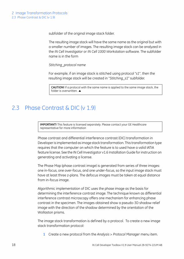
subfolder of the original image stack folder.
The resulting image stack will have the same name as the original but with a smaller number of images. The resulting image stack can be analyzed in the IN Cell Investigator or IN Cell 1000 Workstation software. The subfolder name is in the form
Stitching_protocol name
For example, if an image stack is stitched using protocol "s1", then the resulting image stack will be created in "Stitching_s1" subfolder.
2.3 Phase Contrast & DIC (v 1.9)
Phase contrast and differential interference contrast (DIC) transformation in Developer is implemented as image stack transformation. This transformation type requires that the computer on which the feature is to used have a valid IATIA feature license. See the IN Cell Investigator v1.6 Installation Guide for instruction on generating and activating a license.
The Phase Map (phase contrast image) is generated from series of three images: one in-focus, one over-focus, and one under-focus, so the input image stack must have at least three z-plans. The defocus images must be taken at equal distance from in-focus image.
Algorithmic implementation of DIC uses the phase image as the basis for determining the interference contrast image. The technique known as differential interference contrast microscopy offers one mechanism for enhancing phase contrast in the specimen. The images obtained show a pseudo-3D shadow relief image with the direction of the shadow determined by the orientation of the Wollaston prisms.
The image stack transformation is defined by a protocol. To create a new image stack transformation protocol:
1 Create a new protocol from the Analysis > Protocol Manager menu item.
CAUTION! If a protocol with the same name is applied to the same image stack, the folder is overwritten.
IMPORTANT! This feature is licensed separately. Please contact your GE Healthcare representative for more information
18 IN Cell Developer Toolbox V1.9 User Manual 28-9274-22UM AB
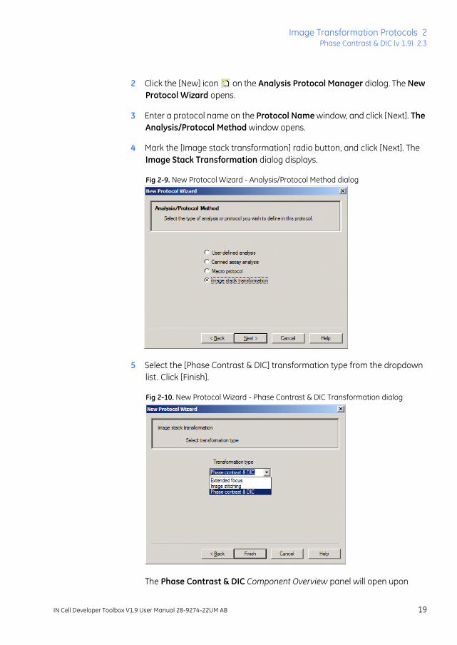
Image Transformation Protocols 2Phase Contrast & DIC (v 1.9) 2.3
2 Click the [New] icon on the Analysis Protocol Manager dialog. The New Protocol Wizard opens.
3 Enter a protocol name on the Protocol Name window, and click [Next]. The Analysis/Protocol Method window opens.
4 Mark the [Image stack transformation] radio button, and click [Next]. The Image Stack Transformation dialog displays.
Fig 2-9. New Protocol Wizard - Analysis/Protocol Method dialog
5 Select the [Phase Contrast & DIC] transformation type from the dropdown list. Click [Finish].
Fig 2-10. New Protocol Wizard - Phase Contrast & DIC Transformation dialog
The Phase Contrast & DIC Component Overview panel will open upon
IN Cell Developer Toolbox V1.9 User Manual 28-9274-22UM AB 19

2 Image Transformation Protocols2.3 Phase Contrast & DIC (v 1.9)
exiting the wizard. The overview panel is divided into 3 sections - Phase Contrast, DIC, and Common Parameters - described in the table below.
Fig 2-11. Phase Contrast & DIC Component Overview panel
Phase Contrast
Parameter Description
High pass filter
Control the amount of detail filtered out of the image. A high pass filter setting of 0 provides the most quantitative image. Increasing the value of the filter removes the lowest frequencies giving an image more composed of boundary or edge detail.
Light Select either transmitted or reflected from the dropdown. Transmitted - produces a conventional transmitted optical microscope image Reflected - produces a conventional reflected optical microscope image
Invert phase
Inverts the polarity of the phase output image; by default is set to OFF. Selecting [On] will invert the phase of the image, where [Off] disables the feature
Preview button
Preview transformation on the current field. The resulting transformation displays in the Preview channel. The field to preview is selected on the Plate Map Viewer.
20 IN Cell Developer Toolbox V1.9 User Manual 28-9274-22UM AB

Image Transformation Protocols 2Phase Contrast & DIC (v 1.9) 2.3
DIC
Common Settings
Parameter Description
Enable Click Yes to enable the DIC feature, or No to disable
Contrast angle
Changes the angle of illumination, which controls the direction of the shadow relief of the DIC image. The default is 150 degree; the acceptable range is 0–360 degrees
Combiner prizm
Defines motion of the Wollaston prismThe default is 0.0; the acceptable range is -90 degree to +90 degree.
Modulation mode
Determines whether the amplitude data is included in the image. Disabled - No modulation with intensity image Standard - Basic modulation with intensity image (multiplied) Enhanced - Enhanced modulation with intensity image (uses Absorption parameter to determine the degree of modulation with the intensity image)
Absorption Enabled when the Modulation Mode = Enhanced The acceptable range is 0–1.0 Absorption effects can be excluded by setting the Modulation mode to "Disabled", a feature not available using conventional microscope DIC optics.
Parameter Description
Wave index
Defines the wave to be transformed. Select wave index from the available wavelengths in the dropdown list for the transformation. The transformation is applied to the selected wavelength only. Any other wavelrngths available for the image in focus are copied to the resulting image. If an image stack is loaded, the wave name is shown instead of the wave index. When the wave index is displayed, it appears as a number.
Focus plane
Use the dropdown to select the correct z-plane in which the image is in focus.
Defocus distance
Defocus distance is the distance from the in-focus images to the over focus and under focus images assumed to be positive and negative defocus steps. Defocus distance is determined as a relative value defined as the number of Z-planes between two consecutive Z-planes.
IN Cell Developer Toolbox V1.9 User Manual 28-9274-22UM AB 21

2 Image Transformation Protocols2.3 Phase Contrast & DIC (v 1.9)
6 Modify the parameters by clicking in the [Value] column to change the parameter values, as described in the tables above.
7 To apply the Phase Contrast & DIC protocol to an image stack,:
a. Click the Preview button to view the resulting transformation displays in the Preview channel for the current well.
b. Run the Analysis by clicking the button and select [Analyze entire stack].
8 If the default output directory is selected, the Phase Contrast & DIC transformation creates a new image stack in a subfolder of the original image stack folder. The resulting image stack will have the same name as the original but contains fewer images. The resulting image stack can be analyzed in the IN Cell Investigator or IN Cell 1000 Workstation software.The subfolder name has the form
PhaseContrast_protocol name
For example, if an image stack in "Tissue" folder is transformed using protocol "p1", then the resulting image stack will be created in "PhaseContrast_p1" subfolder.
Output directory
default or user-defined . The default directory is defined as PhaseContrast_protocol name. Refer to step #8 for detail
Directory name
Enabled when Output Directory =User-defined Use the Browse button to navigate the location to where to save the output image
Update button
Used to update the wavelengthand focus plane list after loading a new image stack..
CAUTION! If a protocol with the same name is applied to the same image stack, the folder is overwritten.
Parameter Description
22 IN Cell Developer Toolbox V1.9 User Manual 28-9274-22UM AB

Pre-processing Operations 3Pseudo Florescence Preprocessing (v 1.7) 3.1
3 Pre-processing Operations
3.1 Pseudo Florescence Preprocessing (v 1.7) Transmitted light images cannot readily be segmented using standard methods. The Pseudo-Fluorescence pre-process tool is specifically designed to convert transmitted light images to pseudo-fluorescent images, which can then be segmented. Improvements to the pseudo-fluorescence tool in IN Cell Developer Toolbox v1.7 make it more adaptable to different levels of image quality.
1 Right-click on the [Preprocessing] node, selecting [Insert as First Preprocess] from the context-sensitive menu, and [Pseudo Florescence] from the sub-menu.
Fig 3-1. Preprocessing Node
The Pseudo Florescence settings display in the Component Settings panel of the Protocol Explorer.
Fig 3-2. Pseudo-Florescence Component Settings Panel
IN Cell Developer Toolbox V1.9 User Manual 28-9274-22UM AB 23
3 Pre-processing Operations3.1 Pseudo Florescence Preprocessing (v 1.7)
2 In the [Method:] field, select from the dropdown list. Each of the methods use intensity gradient information to identify objects (for example, steep gradients in images indicate edges). You may select from:
• Nuclear - aid in the identification of nuclear objects
• Edge - aid in the identification of the edges of objects
• Texture - aid in the identification objects based on differences in their roughness and smoothness.
Note: It is recommended to combine Pseudo Florescence with the "Object" segmentation as this will be adequate for most uses (as a default). Additionally, you can run Pseudo Florescence twice on the same target set using different methods each time.
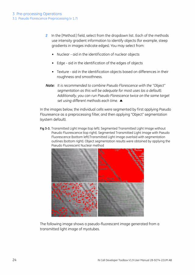
In the images below, the individual cells were segmented by first applying Pseudo Flouresence as a preprocessing filter, and then applying "Object" segmentation (system default).
Fig 3-3. Transmitted Light Image (top left). Segmented Transmitted Light Image without Pseudo Fluorescence (top right). Segmented Transmitted Light Image with Pseudo Fluorescence (bottom left).Transmitted Light Image overlaid with segmentation outlines (bottom right). Object segmentation results were obtained by applying the Pseudo Fluorescent Nuclear method
The following image shows a pseudo-fluorescent image generated from a transmitted light image of myotubes.
24 IN Cell Developer Toolbox V1.9 User Manual 28-9274-22UM AB

Pre-processing Operations 3Pseudo Florescence Preprocessing (v 1.7) 3.1
Fig 3-4. Pseudo-fluorescent rendering of a transmitted light image of myotubes
The effects of processing the image with the different nuclear, edge, and texture methods are shown below.
Fig 3-5. Texture (A), Edge (B), and Nuclear (C) methods applied to transmitted light image of myotubes. Segmented images of Texture method (D), Edge method (E), and Nuclear method (F)
In addition, you can modify the values of the following Parameters using their associated slider keys:
• Sensitivity - increase or decrease contrast
• Deshading radius - increase or decrease the size of artifacts (such as dark bands that will be removed from the image).
Enlarging the deshading radius will result in the Developer software taking longer to run and in small-sized artifacts being ignored though it may be more
IN Cell Developer Toolbox V1.9 User Manual 28-9274-22UM AB 25

3 Pre-processing Operations3.2 Texture Transformation (v 1.8)
noise resistant.
• Edge filter radius - finds sharp contrasts in intensities in an image in order to identify edges.
Decreasing the radius will identify finer lines but at the cost of increased sensitivity to noise.
• Neighborhood radius - increase or decrease the size of the neighborhood used to find edges.
Decreasing the radius gives a more detailed view while increasing the radius gives a more overall view. For example, increasing the radius may make a broken line appear solid.
Note: The results and improvements of Preprocessing are only visible when performing the segmentation under the Preview function or by double-clicking under the segmentation node.
3.2 Texture Transformation (v 1.8) Texture transformations are a group of image processing operations that use image textures to improve segmentation of specific features or can be used to extract texture-specific measurements.
In IN Cell Developer Toolbox, texture transformation are gray-scale image to image transforms that are applied as a preprocess prior to segmentation. The group of algorithms generates the image transform using 'approximate GLCM' method.
1 Right-click on the [Preprocessing] node, selecting [Insert as First Preprocess] from the context-sensitive menu, and [Texture Transformation] from the sub-menu.
26 IN Cell Developer Toolbox V1.9 User Manual 28-9274-22UM AB

Pre-processing Operations 3Texture Transformation (v 1.8) 3.2
Fig 3-6. Preprocessing options - Texture Transformation
The Texture Transform settings display in the Component Settings panel of the Protocol Explorer.
Fig 3-7. Sample Texture Transform panel
2 In the [Transformation:] field, select from the dropdown list.
Transformation Type
Usage
GLCM P_max consolidates locally uniform areas
GCLM Contrast detects intensity changes in the vicinity
GCLM Homogeneity accentuates areas having uniform gray levels
GCLM Mean similar to vicinity averaging
IN Cell Developer Toolbox V1.9 User Manual 28-9274-22UM AB 27

3 Pre-processing Operations3.2 Texture Transformation (v 1.8)
You can modify the values of the parameters using their associated slider keys:
• Kernel size - size of the vicinity; this value is relevant to the size of the object of interest
Marking the [Advanced Parameters] checkbox provides additional parameters:
• Shift - small local spatial variation (deviation), used by GLCM algorithms
• Coefficient - a mutiplier used to standardize the output texture image
• Threshold - a detail contrast choosing tool, that when increased makes the <cos2> algorithm more selective
Following are some examples of texture transformation.
GCLM Energy accentuates areas with small local undulations of grey levels - similar to "Homogeneity
GCLM Entropy value proportional to the nonuniformity of gray levels in the vicinity - similar to "Contrast"
Standard Deviation proportional to the intensity of undulations in the vicinity of pixel of interest
Coefficient of Variation
Coefficient of variation detects undulations relative to the average value
<cos2> local measure of structure (e.g. fibers) ordering, approaching 1 for ordered structure and 0.5 for random intensity field
Transformation Type
Usage
28 IN Cell Developer Toolbox V1.9 User Manual 28-9274-22UM AB

Pre-processing Operations 3Shading Removal QSM (v 1.9) 3.3
Fig 3-8. Example of< cos2> transform
Fig 3-9. Example of GCLM Entropy transform
3.3 Shading Removal QSM (v 1.9) The Shading Removal QSM is used to remove inherent, global variations in background intensity caused by the imaging system's various optical components (e.g., illumination, filters, objective lens). Acquired images may display uneven illumination distribution near the image centre as the intensity diminishes on approaching the image border. Correction for this uneven illumination is essential for any further image operation to produce better image quality. A preprocessing step is required to correct for this uneven illumination.
Shading Removal QSM computes the background shading non-uniformity for each sample image separately. The image is corrected through iterative fitting of the best surface to the image background.
1 Right-click on the [Preprocessing] node, selecting [Insert as First Preprocess] from the context-sensitive menu, and [Shading Removal QSM] from the sub-menu.
Ordered Disordered
F-Actin
cos2 texture
IN Cell Developer Toolbox V1.9 User Manual 28-9274-22UM AB 29

3 Pre-processing Operations3.3 Shading Removal QSM (v 1.9)
Fig 3-10.
The Shading Removal QSM settings display in the Component Settings panel of the Protocol Explorer.
Fig 3-11. Shading Removal QSM Component Settings
2 Modify the parameters by clicking in the text fields, as described below.
% Pixels for Initial Estimation
Specify the percent of initial background pixels to be used for surface fitting, where background points are defined as a set of pixels from the original image used to estimate the model parameters to generate surface. The default value of 100 represents that 100% of ther image pixels to be considered as background points, whereas a value of 50 selects only 50% of the original image pixels for estimating the surface coefficients.
Maximum # Iterations
Number of iterations allowed before the process is terminated prior to reaching convergence. The default value is 50; the value range is 2-100.
30 IN Cell Developer Toolbox V1.9 User Manual 28-9274-22UM AB

Pre-processing Operations 3Shading Removal QSM (v 1.9) 3.3
3 Mark the checkboxes to enable:
• Save output images - to save surface & corrected images generated after last iteration The corrected image is saved as <Image stack Folder>\FFCQSM_Corrected The surface image is saved as <Image stack Folder>\FFCQSM_Background
• Advanced Parameters - Selecting this parameter displays the two following parameters. Otherwise, the following two parameters are set to their default values.
• Well Wall Removal - Selected by default. If the well wall is detected, the algorithm detects the inner well wall and calculates the best-fit corresponding to the detected well region. Two parameters are available to provide better calculation of the well wall diameter.
• Fill Non-Mask Region with Mean BG Intensity - this parameter is enabled with Well Wall Removal
The algorithm produces a circular mask for the well region and retains the image information from inside the well region only. The regions
Multiplier for BG Points Selection
A constant multiplier of the variance of the corrected image, used to update background pixels for surface fitting during each iteration of the algorithm.The default value is 5. The value ranges from 0.001 to 10000. The value increases or decreases at an order of 10.
Convergence Factor
Multiplier of input image variance used to stop the processing when two consecutive surface values are similar.The default value is 1. The value range is 0.0001 to 1000.
~Well Diameter specifies the approximate diameter of the well wall (inner edge to inner edge). The value defaults to 0.
Diffirential Well Radius
specifies the distance between the outer and inner edges of the well wall (in pixels). Positive values enlarge the differential, whereas negative values decrease the differential. The value defaults to 0.
IN Cell Developer Toolbox V1.9 User Manual 28-9274-22UM AB 31

3 Pre-processing Operations3.3 Shading Removal QSM (v 1.9)
outside the mask are filled with average background intensity, calculated by the Flat Field Correction algorithm. Selection of this check box filles the outside region with average background intensity derived from Shading Removal QSM algorithm
Note: On preview, the output image is displayed in the preview channel. If the output image is not properly visible in the viewer, then manually enhance the visual range to maximum.
32 IN Cell Developer Toolbox V1.9 User Manual 28-9274-22UM AB

Segmentation Operations 4Version 1.7 Updates - Additional Parameters 4.1
4 Segmentation Operations
4.1 Version 1.7 Updates - Additional Parameters Various component setting panels have been updated.
4.1.1 Intensity Segmentation Panel Fig 4-1. Intensity Segmentation Panel
A checkbox for [Use automatic threshold] has been added. When marked, minimum threshold is automatically set for each image (using a method such as Otsu's algorithm). This feature is useful for addressing fluorescent images where a white object displayed on a darker background.
Manual threshold setting can be set by clicking the [Find Target] button to open the Intensity Segmentation Parameters window in which the intensity is set by adjusting the slider.
IN Cell Developer Toolbox V1.9 User Manual 28-9274-22UM AB 33

4 Segmentation Operations4.1 Version 1.7 Updates - Additional Parameters
4.1.2 Vesicle Segmentation Panel (v 1.7) Fig 4-2. Vesicle Segmentation Panel
The following checkboxes have been added:
• [Use octagonal morphology] - improves the speed of the algorithm by trading off some precision. When marked, the analysis algorithm will use an octagonal structuring element (rather than round) for most morphological operations.
• [Sensitivity range] - when marked, allows you to enter a sensitivity value from 1.3 to 100 to adjust the contrast interval used to map the vesicle sensitivity scale. The higher the local contrast in the image (specifically, vesicle to background intensity ratio), the higher the sensitivity range value required. By default, the Sensitivity is set to 1.3 (i.e., the checkbox is not enabled). For most applications, the default setting will not need to be changed.
• [Low background] - used for images acquired by optical z-sectioning or transmitted light images pre-processed by pseudo-fluorescence. Selecting this option automatically shifts image intensity for low background signal images to fit the algorithm.
34 IN Cell Developer Toolbox V1.9 User Manual 28-9274-22UM AB

Segmentation Operations 4Version 1.7 Updates - Additional Parameters 4.1
4.1.3 Nuclear Segmentation Panel Fig 4-3. Nuclear Segmentation Panel
The following checkboxes have been added:
• [Use octagonal morphology] - improves the speed of the algorithm by trading off some precision. When marked the analysis algorithm will use an octagonal structuring element (rather than round) for most morphological operations
• [Sensitivity range] - when marked, allows you to enter a sensitivity from 1.3 to 100 to adjust the contrast interval. By default, the Sensitivity range is set to 1.3 (i.e., the checkbox is not enabled).
• [Precise mask] - when marked, allows for better segmentation results for small objects.
• [Low background] - used for images acquired by optical z-sectioning or transmitted light images pre-processed by pseudo-fluorescence. Selecting this option automatically shifts image intensity for low background signal images to fit the algorithm.
IN Cell Developer Toolbox V1.9 User Manual 28-9274-22UM AB 35

4 Segmentation Operations4.2 Version 1.8 Updates
4.1.4 Cytoplasm Segmentation Panel Fig 4-4. Cytoplasm Segmentation Panel
A checkbox for [Use octagonal morphology] has been added. Selecting this option improves the speed of the algorithm by trading off some precision. When marked, the analysis algorithm will use an octagonal structuring element (rather than round) for most morphological operations.
4.2 Version 1.8 Updates
4.2.1 Shape Sensitive Segmentation within Vesicle Segmentation A Shape Detection option has been added to the Vesicle segmentation method to allow to aid object identification based on their shape. The shapes of objects in the image are detected in the form of peaks and ridges existing in the object.
To set the shape selection parameter:
1 Select [Vesicle segmentation] from the Segmentation method listing. The Vesicle Segmentation panel displays.
36 IN Cell Developer Toolbox V1.9 User Manual 28-9274-22UM AB

Segmentation Operations 4Version 1.8 Updates 4.2
Fig 4-5. Vesicle Segmentation Panel
2 Define the vesicle segmentation parameters. (Refer to the IN Cell Developer Toolbox v1.6 User Manual, and the Shape Sensitive Segmentation within Vesicle Segmentation section above for detail.)
3 At the [Shape detection] field, select a shape criterion from the dropdown list. Those objects that match the criteria will be included in the segmentation result
Note: When selecting either peak or ridge as shape criteria, the overall sensitivity may require adjustment via the [Sensitivity range] parameter to exclude background noise from the shape detection.
Option Description
No constraints
Selects objects to segment indifferent to shape Segment regardless of shape
Peak Selects objects based on detection of long branches
Ridge Segmentation of round shapes and eliminates elongated shapes
Selects objects based on detection of intensity peaks inside objects
IN Cell Developer Toolbox V1.9 User Manual 28-9274-22UM AB 37

4 Segmentation Operations4.3 Version 1.9 Updates
4 View the segmentation results by selecting Segmentation > Preview. The image display will update with the selected shapes included.
Fig 4-6. No constraints on shape detection, peak shape detection, ridge shape detection
4.3 Version 1.9 Updates
4.3.1 DT Watershed SegmentationDT Watershed segmentation is used to segment confluent images, and is implemented using the plug-in interface of IN Cell Developer Toolbox. The algorithm library takes as input gray scale images and outputs binary images.
1 Confirm that the segmentation algorithm was loaded.
Enable the DT Watershed segmentation plug-in module. Refer to Section 11.2.1 Plug-in Interface for instruction on configuring plugin algorithms using the Plugin Interface.
2 From the [Segmentation] node, select [Change Segmentation Type] from the context-sensitive menu. The DT Watershed operation should display in the list.
Fig 4-7. Segmentation Options - DT Watershed
The DT Watershed Segmentation panel displays.
38 IN Cell Developer Toolbox V1.9 User Manual 28-9274-22UM AB

Segmentation Operations 4Version 1.9 Updates 4.3
Fig 4-8. DT Watershed Segmentation Panel
The panel contains the following parameters:
The Advanced Parameters for Area Based Object Merging can be used to further define object merging, when the value of the [Min Area] parameter is greater than 0. Objects can be merged with their neighboring regions by supplying values to the parameters described below. The sum of both
Threshold Range
Determines how the object will be segmented. A high value results in under-segmentation, whereas a low value results in over-segmentation, where high and low are relative descriptors.
Min Area Objects with area less than the input value are merged with their neighboring regions. Enter a value in the text box or select a value from the image using drawing tools.
Background Value
Threshold value below which all pixels become part of the background, helping to differentiate between the object and the background. Mark the [Use Automatic] checkbox in the Background Value section to allow the software to automatically determine the background value.
IN Cell Developer Toolbox V1.9 User Manual 28-9274-22UM AB 39

4 Segmentation Operations4.3 Version 1.9 Updates
values for intensity and boundary length must equal 1.
3 Set the parameters as follows to achieve the best image results:
a. Set the background value to capture maximum image information. The [Min Area] should be set to 0, and [Use Region Breaking] check box should be unmarked.
b. Enter a threshold value in the [Threshold Range] field. The setting should provide a minimum of over-segmentation and under-segmentation.
c. If over-segmentation is observed, set the value of the [Min Area] parameter to a value greater than the area of the largest over-segmented region. The Advanced Parameters can be adjusted to enhance the results of the object merging.
d. If under-segmentation is observed, use the [Use Region Breaking] check box to break the under-segmented regions.
4 View the segmentation results by selecting Segmentation > Preview. The image display will update with the selected shapes included.
Intensity Weight
Indicates the use of intensity for object merging (as a percentage). The value range is 0-1, where 1= only intensity is used for object merging, and. 0 =intensity is not be used for object merging.
Boundary Length Weight
Indicates the use of boundary length for object merging (as a percentage). The value range is 0-1, where 1= only boundary length is used for object merging, and. 0 = boundary length is not be used for object merging.
Break Regions Mark the [Use Region Breaking] checkbox in the Break Regions section if under-segmentation is observed in the image. Under-segmented regions of the image are removed.
40 IN Cell Developer Toolbox V1.9 User Manual 28-9274-22UM AB

Post-processing Operations 5Watershed Clump Breaking (v 1.8) 5.1
5 Post-processing Operations
5.1 Watershed Clump Breaking (v 1.8) The aim of watershed breaking is to separate multiple objects clumped together as a single object into segmented images when the targets are so close together that their inter-cellular boundaries are not distinguishable
It requires segmented images as input which can be of the types:
a. Segmented images of both nucleus and cytoplasm
b. Segmented images of nucleus only
c. Segmented images of cytoplasm only
The output is the declumped cytoplasm, declumped nucleus and declumped cytoplasm images., respectively.
Note: The Watershed Clump Breaking algorithm has limitations when the size of the nucleus and cytoplasm are vastly different for confluent cytoplasms.
Watershed Clump Breaking is a 2-phase process:
• Phase 1 (Region Growing)- The algorithm grows region from the distance transform image (generated from segmented image). However, it generates multiple regions even for a single object (cell/nucleus/cytoplasm). The algorithm grows regions on distance transform image, which is generated from segmented image. However, it generates multiple regions even for single objects (nucleus/cytoplasm).
• Phase 2 (Split Merge Analysis) - In this phase, each region is analyzed with respect to its neighboring region and makes a decision whether to merge or retain as it is.
• The final output from the cytoplasm image only is displayed in the image viewer.
Selecting the with Seed postprocess option allows you to select a seed object on which the clump breaking activity should focus (provides a 'search' point). The regions are grown on distance transformed cytoplasmic image using nucleus as the seed.
IN Cell Developer Toolbox V1.9 User Manual 28-9274-22UM AB 41

5 Post-processing Operations5.1 Watershed Clump Breaking (v 1.8)
Note: When applying Watershed Clump Breaking, it is recommended that if the image has any regions containing 'holes', they first be filled using the Fill Holes postprocess option. To apply the Watershed Clump Breaking postprocess:
Fig 5-1. Postprocessing Options - Watershed Clump Breaking options
1 From the Post-processing functions, right click and select Insert as First Postprocess.
2 Watershed clump breaking is based on shape analysis of binary image resulted from segmentation.Hence, there should be some shape information between the adjoining regions to serve as input to the algorithm.
From the list of options, select either:
• [Watershed Clump Breaking] - nucleus segmented image if without seed option chosen
• [Watershed Clump Breaking (With Seed)] - in scenarios when the regions are very densely connected, a seed image is required to provide shape information between adjoining regions.
3 Mark the image and click Postprocessing>Preview or double-click on Postprocessing.
42 IN Cell Developer Toolbox V1.9 User Manual 28-9274-22UM AB

Post-processing Operations 5Watershed Clump Breaking (v 1.8) 5.1
Fig 5-2. Watershed Clump Breaking (without Seed)
In the case of [Watershed Clump Breaking (With Seed)], select the seed image from the dropdown list.
Fig 5-3. Watershed Clump Breaking (With Seed)
IN Cell Developer Toolbox V1.9 User Manual 28-9274-22UM AB 43

5 Post-processing Operations5.1 Watershed Clump Breaking (v 1.8)
Examples of the watershed clump breaking action are displayed below.
Fig 5-4. Examples of watershed clump breaking before and after segmentation
Fig 5-5. Examples of watershed clump breaking following segmentation
5.1.1 Image Types and Processing The image types and their respective processing are described below:
Type Processing Method
Image stacks with both nuclei and cytoplasm
Nuclei are de clumped and cytoplasmic regions are grown based on nucleus.
Operation to be applied here is watershed clump breaking with seed.
Image Stacks with only nucleus
Regions are grown on nucleus images and split merge analysis is applied on region grown images.
Operation to be applied here is watershed clump breaking.
44 IN Cell Developer Toolbox V1.9 User Manual 28-9274-22UM AB

Post-processing Operations 5Fill Holes (v 1.8) 5.2
* holes in the region of the cytoplasm can be distorting, so apply Fill Ho;es postprocess operation before Watershed Clump Breaking If there is no curvature info available, then the nuclei info is exploited in order to grow the region
** intensity within an object is darker than the surrounding pixels, hence creating holes in the object region
5.2 Fill Holes (v 1.8) The Fill Holes postprocessing option is designed to fill any 'holes' that may be present in an object. The algorithm replaces pixels with duplicates of surrounding pixels to fill the blank space or hole. Selecting the option will apply the algorithm and automatically update the image.
1 Mark the image in which you want to apply the Fill Holes postprocess.
2 From the [Postprocessing] functions, right click and select [Insert as First] [Postprocess], and select [Fill Holes] from the list of options.
The user need not supply any parameters so the Component Overview panel displays blank.
3 To view the 'filled' image, click Postprocessing>Preview or double-click on Postprocessing.
Image Stacks with only cytoplasm images (single nuclei)
Regions are grown on cytoplasm images and split merge analysis is applied on region grown images.
Operation to be applied here is watershed clump breaking.
Image Stacks with cytoplasm images with multiple nuclei per cytoplasm
Regions are grown on cytoplasm images and split merge is applied on region grown images.
Operation to be applied is watershed clump breaking
Images with holes inside the region
Process for fill holes and then
apply Watershed Clump Breaking **
White Border Images
Have bright cellular boundary creating 'holes' in the region, so process for Fill Holes and
apply watershed Clump breaking
Type Processing Method
IN Cell Developer Toolbox V1.9 User Manual 28-9274-22UM AB 45

5 Post-processing Operations5.3 Border Object Removal (v 1.8)
Fig 5-6. Fill Holes algorithm: (A) original image, (B) image after Fill Holes algorithm has been applied
5.3 Border Object Removal (v 1.8) The Border Object Removal post-processing tool is applied to the segmentation result to remove partially visible objects or objects neighboring with the border or objects that are too close to the margins that will be too difficult to analyze.
Fig 5-7. Border Object Removal panel
To apply the Border Object Removal post-process option:
1 From the Post-processing functions, select Insert as First Postprocess, select the [Border Object Removal] option from the list.
2 Mark the radio button for the type of exclusion to perform:
A B
46 IN Cell Developer Toolbox V1.9 User Manual 28-9274-22UM AB
Post-processing Operations 5Border Object Removal (v 1.8) 5.3
• [Remove all objects touching borders] - All objects that are touching the borders are removed
• [Remove all objects within specified distance from borders] - The objects are removed accordingly for distance specified from a border(s). The [Distance] field will be enabled when this option is selected.
The distance from the border can be defined as a distance from a border to the nearest pixel of the object's edge.
3 Mark the checkbox(es) for the specific directional from which you want to have objects removed.
• [All Borders] - All objects that are touching the borders are removed. All Borders is set as the default direction.
• To enable the individual directional options, unmark the [All borders] checkbox. Refer to Section 5.3.1, for description of directional choices.
Note: When selecting individual directional options, one or more directions may be selected (e.g., mark left, right to have objects removed from those borders only).
4 Enter a value in the [Distance] text field to specify the distance (in pixels) from which objects should be removed from the border. Conversely, use the slider to select the distance.
IN Cell Developer Toolbox V1.9 User Manual 28-9274-22UM AB 47

5 Post-processing Operations5.3 Border Object Removal (v 1.8)
5.3.1 Border Object Removal Combinations Removal Option Directional Option Description
Objects touching borders
Remove all objects that touch" and "Left
objects that touch at the left are removed
Remove all objects that touch" and "Right
objects that touch at the right are removed
Remove all objects that touch" and "Bottom
objects that touch at the bottom are removed
Remove all objects that touch" and "Top
objects that touch at the top are removed
Objects within distance from borders
Remove all objects within distance from borders" and "Left
objects are removed by the distance specified from left border
Remove all objects within distance from borders" and "Right
objects are removed by the distance specified from right border
Remove all objects within distance from borders" and "Top
objects are removed by the distance specified from top border
Remove all objects within distance from borders" and "Bottom
objects are removed by the distance specified from bottom border
48 IN Cell Developer Toolbox V1.9 User Manual 28-9274-22UM AB

Classifiers in Developer Toolbox (v 1.7) 6
6 Classifiers in Developer Toolbox (v 1.7)
The IN Cell Developer Toolbox Classifiers function offers the ability to classify objects in the image (targets) into multiple sub-populations. This flexible function makes it easier to develop analysis protocols that automatically assign cells to pre-defined classes. The protocol used for automatic classification is called a classifier (may also be referred to as a classification protocol).
Classifiers can be set using any previously defined measure, thus allowing targets to be classified using any combination of measures. To define measures:
1 Right-click the Measures node under the desired target set.
(For more detail, refer to Chapter 5, Measurement Definition in IN Cell Developer Toolbox V1.7 High-content image analysis software User's Reference Manual.
Fig 6-1. Selecting the Measures node in a protocol
2 To define a classifier, click the Classifiers node in the Component Overview section of the Protocol Explorer. The Classifier settings area displays.
IN Cell Developer Toolbox V1.9 User Manual 28-9274-22UM AB 49

6 Classifiers in Developer Toolbox (v 1.7)6.1 Classification using a Threshold filter
Fig 6-2. Classifiers Area. Right-click and select New Threshold
3 Right-clicking within this pane opens a context-sensitive menu with the following options:
• New Threshold: classification into two sub-populations based on a simple threshold of any chosen measurement.
• New Linear Discriminant: creation of up to four sub-populations based on a 2D scatter plot of any two measurements
• New Decision Tree: enables complex classification schemes by combining the Threshold and Discriminant filters
Each classifier can be configured by selecting appropriate measures and by using interactive graphs.
6.1 Classification using a Threshold filter The Threshold filter allows for the division of populations into two sub-populations based on a single measure. Use a threshold filter to define:
• Cells having object measures above or below threshold values.
• Cells having object measures that fall within a range of values.
In the Classifier settings area:
1 Right-click to open the context-sensitive list and click [New Threshold] to display the Threshold window
50 IN Cell Developer Toolbox V1.9 User Manual 28-9274-22UM AB

Classifiers in Developer Toolbox (v 1.7) 6Classification using a Threshold filter 6.1
Fig 6-3. Threshold Filter window
2 Provide a title for the filter (optional), and click to display a list of available measures.
(Note that only measures selected in the Measures Selection or created in the Edit User Defined Measure dialog will appear on this list). Highlight the required measures in the list, and then click [Select].
Note: If you previously selected an analyzed well in the Image Stack window, before adding the filter, a histogram will appear in the Threshold window.
3 Enter the required information in the context-sensitive fields that appear when you select one of the following options:
• above or below - enter the threshold above or below which the measurement must be must be in order for the cell to be filtered
• in range - enter the lower and upper limits within which the measurement must fall in order for the cell to be filtered
4 Once sample wells have been analyzed, the histogram will be populated. The threshold(s) can then be adjusted selecting [Edit] and dragging the threshold line(s) to the required position. The resulting value(s) will then be displayed in the Classifier settings area of the Threshold window.
IN Cell Developer Toolbox V1.9 User Manual 28-9274-22UM AB 51

6 Classifiers in Developer Toolbox (v 1.7)6.1 Classification using a Threshold filter
Alternatively, values can be entered manually in the appropriate field(s) in the Classifier area. In the example shown below, sample wells have been analyzed to populate the histogram and the threshold has been set to show two populations based on a threshold value of 1.04 for Nuc/Cell Intensity (Cells).
Fig 6-4. Analysis Protocol Editor. Threshold Filter window showing populated histogram data for Nuc/Cell Intensity (Cells)
5 Select the [Graph] button to access the graphing options in the Histogram window. You can set
• Data display range - the range available for the axis can be set to Automatic (default setting) or Manual by unmarking the checkbox. The manual activates the Min and Max fields where threshold values can be entered.
• Histogram bins - the bin size for each histogram bar can be set to Automatic (default setting) or Manual by unmarking the checkbox. This activates the bin width field in which a more appropriate value can be entered.
52 IN Cell Developer Toolbox V1.9 User Manual 28-9274-22UM AB

Classifiers in Developer Toolbox (v 1.7) 6Classification using a Threshold filter 6.1
Fig 6-5. Threshold filter: Graph options window
Note: Manually selected settings are not saved from a prior invocation of the Histogram window and will revert to Automatic when the graph options are next accessed.
6 Select the [Classes] button to access the Class definition window containing the following options:
• Color - the color of each class can be changed by right-clicking on the color box and selecting a color from the displayed list.
• Class - the class name can be changed by double-clicking on the current name and entering a new name.
• Symbol - the symbol can be changed by double-clicking on the current symbol and entering a new symbol.
• Area - refers to the specified classification regions (not editable).
Fig 6-6. Threshold filter: Class definition window
IN Cell Developer Toolbox V1.9 User Manual 28-9274-22UM AB 53

6 Classifiers in Developer Toolbox (v 1.7)6.2 Classification using a Linear Discriminant Filter
7 Ensure that the name and symbol you have entered corresponds to the correct area (1 or 2) shown in the class definition window.
Note: Though visible, the [Hide Parent] button is disabled in this feature.
6.2 Classification using a Linear Discriminant Filter For the Linear Discriminant filter a scatter plot of any two available measures is generated, enabling cells to be classified into 2, 3 or 4 user-defined populations. This classifier is useful for applications where distinct sub-populations can be discriminated on the basis of two parameters (e.g., an assay where two different fluorescent dyes are used to mark live and dead cells).
1 In the Classifier settings area, right-click to display the context-sensitive menu and select [New Linear Discriminant] to display the Scatter Plot window.
Fig 6-7. Classifiers Area. Right-click and select New Linear Discriminant
54 IN Cell Developer Toolbox V1.9 User Manual 28-9274-22UM AB

Classifiers in Developer Toolbox (v 1.7) 6Classification using a Linear Discriminant Filter 6.2
Fig 6-8. Analysis Protocol Editor. Linear Discriminant 2D (scatter plot) window
2 Enter a name in the [Title] field and click to display a list of available measures that can be specified for the X-axis. Highlight the required measure in the list, and click [Select].
3 Repeat for the Y-axis, selecting the required measure.
Note: In order for the scatter plot to be populated, the sample wells will need to have been analyzed with the selected measures. The example is a Linear Discriminant 2D filter window showing analyzed data
4 Select the [Graph] button to access the Graph options window.
IN Cell Developer Toolbox V1.9 User Manual 28-9274-22UM AB 55
6 Classifiers in Developer Toolbox (v 1.7)6.2 Classification using a Linear Discriminant Filter
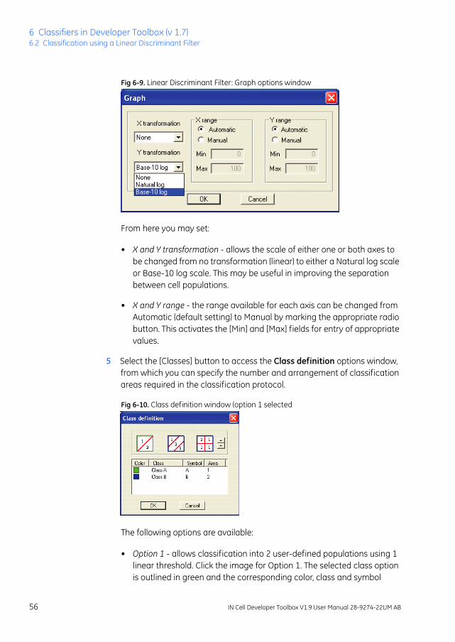
Fig 6-9. Linear Discriminant Filter: Graph options window
From here you may set:
• X and Y transformation - allows the scale of either one or both axes to be changed from no transformation (linear) to either a Natural log scale or Base-10 log scale. This may be useful in improving the separation between cell populations.
• X and Y range - the range available for each axis can be changed from Automatic (default setting) to Manual by marking the appropriate radio button. This activates the [Min] and [Max] fields for entry of appropriate values.
5 Select the [Classes] button to access the Class definition options window, from which you can specify the number and arrangement of classification areas required in the classification protocol.
Fig 6-10. Class definition window (option 1 selected
The following options are available:
• Option 1 - allows classification into 2 user-defined populations using 1 linear threshold. Click the image for Option 1. The selected class option is outlined in green and the corresponding color, class and symbol
56 IN Cell Developer Toolbox V1.9 User Manual 28-9274-22UM AB

Classifiers in Developer Toolbox (v 1.7) 6Classification using a Linear Discriminant Filter 6.2
options become available. These can be changed to more relevant descriptions (as described in Classification using a Threshold filter).
• Option 2 - allows classification into 3 user-defined populations (including 1 unclassified) using 2 parallel linear thresholds. Click the image for Option 2. The selected class option is outlined in green and the corresponding color, class and symbol options become available. These can be changed to more relevant descriptions (as described in Classification using a Threshold filter).
Fig 6-11. Class definition window (option 2 selected)
• Option 3 - allows classification into 2, 3 or 4 user-defined populations using 2 intersecting linear thresholds. Click the image for option 3. Using the associated arrow keys to specify the number of populations (up to 4) and their position (layout) on the resulting scatter plot (for the 2 population option only). The corresponding color, class and symbol options are then available and can be changed to more relevant descriptions (as described in Classification using a Threshold filter).).
IN Cell Developer Toolbox V1.9 User Manual 28-9274-22UM AB 57

6 Classifiers in Developer Toolbox (v 1.7)6.2 Classification using a Linear Discriminant Filter
Fig 6-12. Class definition window (option 3 selected). (A) 2 classes, (B) 3 classes or (C) 4 classes can be defined for the areas specified
6 The linear threshold can then be manually moved by clicking and dragging the threshold line to the required position to specify individual classes of cells. Making changes to the position of the linear threshold requires the changes be reflected on the scatter plot:
• Select Refresh on the Scatter Plot window to update the plot so that all data points within the same area have the same color.
• Select Reset on the Scatter Plot window to reset the position of the linear thresholds to their original defined positions.
Note: Due to the way in which the linear threshold functions, the preferred method is to move the threshold to the required position and click [Refresh] to update the color, name and symbol options.
7 To check the identity of a particular cell, and therefore, to which population it should belong, click on it's corresponding data point (colored dot) on the scatter plot. The corresponding cell will be highlighted in the image and table view. It is important to try different combinations of measures to achieve the best separation between classes.
Note: To view this interaction between the scatter plot data point and a cell in the image, the Sample window must be open. To do this, click the
58 IN Cell Developer Toolbox V1.9 User Manual 28-9274-22UM AB

Classifiers in Developer Toolbox (v 1.7) 6Classification Using a Decision Tree Filter 6.3
[Sample] button on the [Operations] shortcut bar.
8 Click [OK] to close the Linear Discriminant Filter window and save the parameters.
6.3 Classification Using a Decision Tree Filter The Decision tree filter allows you to classify cells into multiple populations based on any available measure. The tree design provides a multi-level structure allowing a cell population to be divided into two sub-populations at each decision point. At each decision point, either one or both populations can be further classified into additional sub-populations or can be reported in the Summary data.
The two types of filter described earlier, Threshold and Linear Discriminant , are available at each decision point, and can also be used in combination.
1 For each Decision Tree filter you want to define, right-click in the [Classifiers] area to display the context-sensitive menu and select [New Decision Tree] to display the Decision tree window.
Fig 6-13. Classifiers Area. Right-click and select New Decision Tree
IN Cell Developer Toolbox V1.9 User Manual 28-9274-22UM AB 59

6 Classifiers in Developer Toolbox (v 1.7)6.3 Classification Using a Decision Tree Filter
Fig 6-14. Decision tree window
2 Add nodes to the tree clicking and dragging a node type from the list to the right of the design pane. The available nodes types are:
The first node in the tree must be a start node - either a threshold or scatter plot node. A decision tree can have only one start node. Secondary nodes of the defined type (either threshold or scatter plot) are then added to build the decision tree.
Note: A node can be added and defined immediately, or all required nodes can be added at once and then defined.
Note: Only two class options are available for Linear Discriminant Class definition filter window when selected within a Decision tree. The
Node Description
Start node T - threshold node to be used as first node in a decision tree. Output populations are labeled as 0 and 1.
Start node S - scatter plot node to be used as the first node in a decision tree. Output populations are labeled as A and B.
Node T - secondary threshold node. Output populations are labeled as 0 and 1
Node S - secondary scatter plot node. Output populations are labeled as A and B
60 IN Cell Developer Toolbox V1.9 User Manual 28-9274-22UM AB

Classifiers in Developer Toolbox (v 1.7) 6Classification Using a Decision Tree Filter 6.3
example shows a Linear Discriminant Filter, Class Definition window when selected within Decision tree
To define nodes:
1 Right click on each node and select the [Edit node] option. Depending on the type selected, a Threshold or Linear Discriminant filter window will display to define the populations.
Each filter will then divide the population into two sub-populations based on the required measures. Refer to the sections, Classification Using a Threshold filter and / or Classification Using a Linear Discriminant filter for detail on defining the filters.
Fig 6-15. Decision tree window showing scatter plot decision nodes
2 Once the start node has been defined, the populations can be further divided into sub-populations. Place the cursor over the primary node, and
IN Cell Developer Toolbox V1.9 User Manual 28-9274-22UM AB 61

6 Classifiers in Developer Toolbox (v 1.7)6.3 Classification Using a Decision Tree Filter
click-and-drag to draw a connecting arrow from the sub-population of the start node to the secondary node.
A connecting line will appear linking the two nodes. In the example below, population 0 will be reported in the summary data and population 1 will be separated into two additional populations (A and B) based on the filter defined by the secondary node.
Fig 6-16. Analysis Protocol Editor. Decision tree window showing Threshold start node and Linear Discriminant 2D secondary node. Population 0 will be reported and population 1 will be further separated into populations A and B
3 Right-clicking on these secondary nodes, in turn, opens threshold or scatter plot filter (as appropriate) to define additional sub-populations.
Note: When defining each decision node within a Decision tree, it is important to rename and change the symbol assigned to each population so they are correctly reported and identified in the summary data table. Names and symbols must be unique for each population. Duplication will result in an error message when the Decision tree window is closed.
62 IN Cell Developer Toolbox V1.9 User Manual 28-9274-22UM AB
Cell Tracking in Developer Toolbox (v 1.7) 7Overview 7.1
7 Cell Tracking in Developer Toolbox (v 1.7)
7.1 Overview Tracking the movement and behavior of living cells is an indispensable technique for a wide variety of functional studies. The images are acquired as a time series by an instrument that allows time-lapse microscopy (e.g., the GE Healthcare IN Cell Analyzer platforms). When applied to these images, the cell tracking feature enables automated quantification of cell position, speed and direction as a function of time. In addition, daughter cells resulting from cell divisions are identified and tracked. Changes in individual cell parameters such as size, shape and intensity are monitored to provide a deeper understanding of the time-dependent behavior of every cell in a population.
You can incorporate cell tracking either into a Multi Target Analysis protocol (refer to Chapter 4, Canned Assay Analysis of the IN Cell Developer Toolbox User Manual for more detail) or into any Developer Toolbox user-defined protocol.
7.2 Cell Tracking Dialog Use the Protocol Explorer to add cell tracking to the analysis protocol.
1 Right-click [Dynamic Behavior], and select [Cell Tracking] from the menu.
The movements of individual cells are tracked using user-selectable methods.
IN Cell Developer Toolbox V1.9 User Manual 28-9274-22UM AB 63

7 Cell Tracking in Developer Toolbox (v 1.7)7.2 Cell Tracking Dialog
Fig 7-1. Cell Tracking
The Cell Tracking panel displays.
Fig 7-2. Cell Tracking Component Overview panel (version 1.7)
7.2.1 Setting Cell Tracking Parameters 1 Set the Cell Tracking parameters as described in the following table. Note
that some fields are disabled depending upon the tracking method selected.
64 IN Cell Developer Toolbox V1.9 User Manual 28-9274-22UM AB

Cell Tracking in Developer Toolbox (v 1.7) 7Cell Tracking Dialog 7.2
Table 7.1. Description of tracking options
2 Click [Change] under the More Options field to further refine the tracking algorithm by setting weights for the different measures used to track cells. Setting a higher weight for a measure gives the measure more importance. The Advanced Tracking Options dialog opens.
Field Description
Track Target Set From the drop-down list, select the Target Set you want to track. When selecting a linked target set, you will be able to specify which component of the linked set will be used for tracking (TargetLink/TargetA or TargetLink/TargetB)
Use Intensity as extra tracking
Enables the use of the Intensity parameter to refine tracking targets.)
Use Area as additional tracking
Enables the use of the Area parameter to refine tracking targets.
Use Morphology (Major axis, Minor axis, Direction) as additional tracking
Enables the use of shape parameters to refine tracking targets.
More Options Click the Change button to open the Advanced Tracking Options dialog (see below)
Relative Threshold (disabled with Particle Filter)
The radius within which objects are considered as potential parents. Setting the value to a large number will result in too many "division" events
Outlier Detection (disabled with Particle Filter)
This threshold value excludes matches that are considerably longer than the majority of matches Small values will lead to many "new" objects, large values will increase the number of "collisions"
Tracking Method Proximity - Track cells based on distances from their previous positions.
Particle Filter - select the number of particles (or points) around an object to search from
Number of particles (disabled with Proximity)
Specify the number of particles for the Particle Filter algorithm
IN Cell Developer Toolbox V1.9 User Manual 28-9274-22UM AB 65

7 Cell Tracking in Developer Toolbox (v 1.7)7.2 Cell Tracking Dialog
Fig 7-3. Advanced Tracking Options Dialog
3 To set a weight:
a. Click the checkbox of the desired measure. The measure is highlighted. By default, the checkboxes for [Pos X] and [Pos Y] are always checked. If your cells preferably move to X or Y decrease the weight of the preferred direction.
b. In the Weight column, drag the slider bar to set the desired value or enter the value in the textbox to the right of the slider. Values may range from 0 (no weight) to 1 000 (most weight). More weight should be given to those attributes that help to differentiate the cells.
Table 7. 2. Cell Tracking Measures
Measure Description
Pos X X location; default marked
Pos Y Y location; default marked
Area Area of the target; Using area as additional tracking marks this checkbox
Dens - Levels Gray-level mean intensity; Using intensity as additional tracking also marks this checkbox
66 IN Cell Developer Toolbox V1.9 User Manual 28-9274-22UM AB

Cell Tracking in Developer Toolbox (v 1.7) 7Cell Tracking Dialog 7.2
Measurements that you specify or create for the tracked target also appear in the dialog. You can optionally select any or all additional tracking factors. Selecting a tracking factor automatically checks the checkbox for the same option in the Cell Tracking dialog and vice versa.
7.2.2 Setting the Tracking Method (updated v1.8) 1 From the [Tracking Method] field on the Cell Tracking Settings dialog, select
a method.:
• The proximity method tracks objects based on their distances between two time points. For a given time point the proximity method tries to match every object to the closest object at the previous time point.
The distance of the two objects is calculated from their position in a multi-dimensional space. If only X and Y positions are chosen as tracking parameters the distance equals the spatial distance, but if additional parameters (e.g. morphology, see below) are included the distance is calculated from the resulting vectors.
The following displays in the Component Settings dialog for Cell Tracking, when the proximity method is selected
Major Axis Length
Longest diameter of the target; Using morphology as additional tracking also marks this checkbox when all 3 are grouped
Minor Axis Length
Shortest diameter of the target; Using morphology as additional tracking also marks this checkbox when all 3 are grouped
Major Axis Angle
Angle of the Major axis with respect to the X axis; Using morphology as additional tracking also marks this checkbox when all 3 are grouped
Measure Description
IN Cell Developer Toolbox V1.9 User Manual 28-9274-22UM AB 67

7 Cell Tracking in Developer Toolbox (v 1.7)7.2 Cell Tracking Dialog
Fig 7-4. Cell Tracking - Proximity dialog
Supply both Relative Threshold and Outlier Detection values on which to calculate the proximity. These fields are enabled on selecting the Proximity tracking method.
• Introduced in Version 1.8, the particle filter method allows the user to select the number of particles (or points) around an object to search from. The Particle Filter tracking method is a Monte Carlo based tracking method.
The following displays in the Component Settings dialog for Cell Tracking when particle filter method is selected.
Fig 7-5. Cell Tracking - Particle Filter dialog
68 IN Cell Developer Toolbox V1.9 User Manual 28-9274-22UM AB

Cell Tracking in Developer Toolbox (v 1.7) 7Labels and Linked Track IDs 7.3
Supply the Number of Particles on which to calculate the proximity. This field is enabled on selecting the Particle Filter tracking method.
7.3 Labels and Linked Track IDs Cells entering the field of view are assigned a label and linked track ID. The label is an ID for a unique cell, whereas the linked track ID allows associates child cells to their parent cells after division. The behavior of labels and linked track ID is illustrated in the following tables.
The following table shows three cells entering the field of view. The cells are assigned labels and linked track IDs of 1, 2, and 3. For two time points, all three cells are in the field of view. For the third time point, cell 2 has left the field of view.
Table 7.3. Label and Linked Track ID for normal moving cells
The next table shows three cells entering the field of view at time 0. The cells are assigned labels 1, 2, and 3 and link track IDs 1, 2, and 3. At time 3000, cell 1 has divided into two daughter cells. Cell 1 is not shown for time 3000. The daughter cells are assigned labels 4 and 5 and linked track ID 1.
Target Set Section Label Linked Track ID Time
nuclei A - 1 (0) 1 1 0
nuclei A - 1 (0) 2 2 0
nuclei A - 1 (0) 3 3 0
nuclei A - 1 (3000) 1 1 3000
nuclei A - 1 (3000) 2 2 3000
nuclei A - 1 (3000) 3 3 3000
nuclei A - 1 (6000) 1 1 6000
nuclei A - 1 (6000) 3 3 6000
IN Cell Developer Toolbox V1.9 User Manual 28-9274-22UM AB 69

7 Cell Tracking in Developer Toolbox (v 1.7)7.3 Labels and Linked Track IDs
Table 7.4. Label and Linked Track ID for dividing cells
The table below shows three cells entering the field of view at time 0. The cells are assigned labels 1, 2, and 3 and linked track IDs 1, 2, and 3. At time 3000, cells 1 and 2 aggregate. Cells 1 and 2 are not shown for time 3000. The aggregate cells are assigned label 4 and linked track ID 4.
Table 7.5. Label and Linked Track ID for aggregating cells
The cell tracking feature works optimally for hundreds of cells per field of view (depending on the magnification, cell speed, and cell density). The acquisition speed of the time-lapse microscopy instrument should be adjusted so that fast moving, as well as slow moving, cells can be imaged.
Note: The ability to track cells accurately will depend critically on cell density (average distance between cells), speed of cell movement, magnification and sampling rate. The sampling rate (time between two images) has to be shorter for fast moving cells or cells at high density. Tracking is most accurate if the average distance traveled between two time points is considerably smaller than the average distance between cells. Selecting additional tracking parameters (e.g. intensity or morphology) will only improve tracking if they are likely to change less between two time points than the X and Y
Target Set Section Label Linked Track ID Time
nuclei A - 1 (0) 1 1 0
nuclei A - 1 (0) 2 2 0
nuclei A - 1 (0) 3 3 0
nuclei A - 1 (3000) 2 2 3000
nuclei A - 1 (3000) 3 3 3000
nuclei A - 1 (3000) 4 1 3000
nuclei A - 1 (3000) 5 1 3000
Target Set Section Label Linked Track ID Time
nuclei A - 1 (0) 1 1 0
nuclei A - 1 (0) 2 2 0
nuclei A - 1 (0) 3 3 0
nuclei A - 1 (3000) 3 3 3000
nuclei A - 1 (3000) 4 4 3000
70 IN Cell Developer Toolbox V1.9 User Manual 28-9274-22UM AB

Cell Tracking in Developer Toolbox (v 1.7) 7Cell Tracking Data Output 7.4
coordinates.
7.4 Cell Tracking Data Output In addition to the measurements specified by the user, the following cell tracking results are always displayed in a data table:
Table 7.6. Default tracking output measures
Parameter Description
Intensity Mean gray level intensity of the chosen target (e.g. cell)
Area Area of the chosen target
XPos X position of the chosen target
YPos Y position of the chosen target
Major Axis Long diameter of the chosen target (usually measured in microns)
Minor Axis Short diameter of the chosen target (usually measured in microns)
Label Label assigned to the chosen target
Linked Track ID Label of original the chosen target
Tracking Distance
Spatial distance that tracked cell has moved between two time points
Polar Angle Measure of direction of moving the chosen target
Tracking Event None = normal translocation New = new entry to field of view Removed = cell exiting from field of view
Collision = cells aggregate Division = cells dividing
Time Index Index to a time point in a time series
Confidence Estimated measure of certainty that a given tracked cell is the same as the original cell. A value closer to 1 indicates a large degree of confidence that the tracker is locked on target, as opposed to a value closer to 0 that indicates a lesser degree of confidence
IN Cell Developer Toolbox V1.9 User Manual 28-9274-22UM AB 71
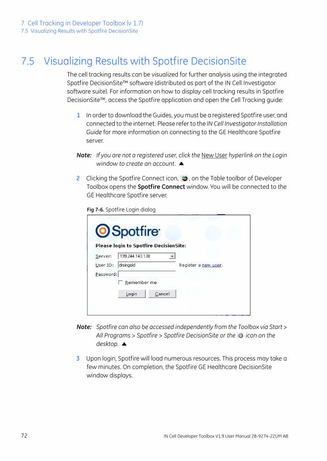
7 Cell Tracking in Developer Toolbox (v 1.7)7.5 Visualizing Results with Spotfire DecisionSite
7.5 Visualizing Results with Spotfire DecisionSite The cell tracking results can be visualized for further analysis using the integrated Spotfire DecisionSite™ software (distributed as part of the IN Cell Investigator software suite). For information on how to display cell tracking results in Spotfire DecisionSite™, access the Spotfire application and open the Cell Tracking guide:
1 In order to download the Guides, you must be a registered Spotfire user, and connected to the internet. Please refer to the IN Cell Investigator Installation Guide for more information on connecting to the GE Healthcare Spotfire server.
Note: If you are not a registered user, click the New User hyperlink on the Login window to create an account.
2 Clicking the Spotfire Connect icon, , on the Table toolbar of Developer Toolbox opens the Spotfire Connect window. You will be connected to the GE Healthcare Spotfire server.
Fig 7-6. Spotfire Login dialog
Note: Spotfire can also be accessed independently from the Toolbox via Start > All Programs > Spotfire > Spotfire DecisionSite or the icon on the desktop.
3 Upon login, Spotfire will load numerous resources. This process may take a few minutes. On completion, the Spotfire GE Healthcare DecisionSite window displays.
72 IN Cell Developer Toolbox V1.9 User Manual 28-9274-22UM AB

Cell Tracking in Developer Toolbox (v 1.7) 7Visualizing Results with Spotfire DecisionSite 7.5
Fig 7-7. Spotfire GE Healthcare DecisionSite window
Note: At initial login, you will be presented with 4-5 security warning messages. To install/download the Cell Tracking Guides from the GEHC SF server, you must accept each by clicking [Run].
Note: Once you have installed the guides you will also be able to use them offline. But you will need to locally log into Spotfire for them to work.
4 Expand the GE Healthcare Guides item and select [Cell Tracking] and the [Cell Tracking] guide. You may also access the guide from the menu via Guides | GE Healthcare Guides | Cell Tracking | Cell Tracking.
IN Cell Developer Toolbox V1.9 User Manual 28-9274-22UM AB 73

7 Cell Tracking in Developer Toolbox (v 1.7)7.5 Visualizing Results with Spotfire DecisionSite
Fig 7-8. Spotfire Guides Menu
The Cell Tracking Guide explains how to create scatter plots and histograms of your data. Upon making your selection, the guide will open displaying the requested data in the graph. Select either of the following to open a view:
• [Open demonstration data and create Cell Track View] - opens stored data within the Guide
• [Create Cell Track View using data loaded from Investigator] - process data you have transferred to Spotfire using the SpotfireConnect function of Investigator
Fig 7-9. Spotfire DecisionSite window
74 IN Cell Developer Toolbox V1.9 User Manual 28-9274-22UM AB
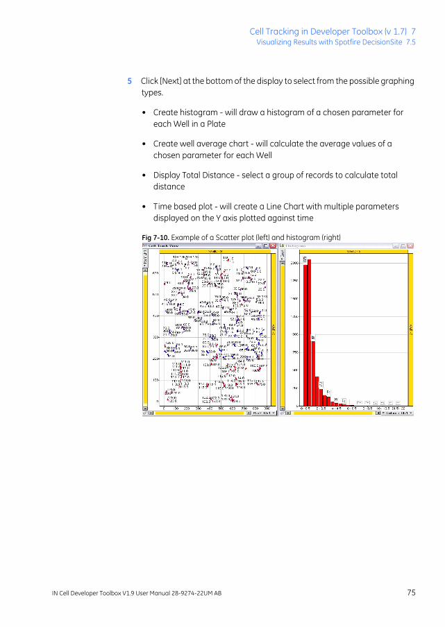
Cell Tracking in Developer Toolbox (v 1.7) 7Visualizing Results with Spotfire DecisionSite 7.5
5 Click [Next] at the bottom of the display to select from the possible graphing types.
• Create histogram - will draw a histogram of a chosen parameter for each Well in a Plate
• Create well average chart - will calculate the average values of a chosen parameter for each Well
• Display Total Distance - select a group of records to calculate total distance
• Time based plot - will create a Line Chart with multiple parameters displayed on the Y axis plotted against time
Fig 7-10. Example of a Scatter plot (left) and histogram (right)
IN Cell Developer Toolbox V1.9 User Manual 28-9274-22UM AB 75
7 Cell Tracking in Developer Toolbox (v 1.7)7.5 Visualizing Results with Spotfire DecisionSite
76 IN Cell Developer Toolbox V1.9 User Manual 28-9274-22UM AB

Data Output 8Updates in v1.8/1.9 8.1
8 Data Output
Once an image stack has been analyzed, the Group Summary table can be used to aggregate the resulting data based on a hierarchy of user-selectable criteria. It is a more flexible alternative to the summary data definition in the Measures dialog (for more detail refer to Chapter 5, Measurement Definition in IN Cell Developer Toolbox V1.7 High-content image analysis software User's Reference Manual, part number 28-4088-71). The Group Summary table provides the only option for summarizing sub-population data created by Classifiers.
8.1 Updates in v1.8/1.9The IN Cell Developer Toolbox data output feature has been updated in version 1.8 to include:
• Ability to import plate descriptions (Plate ID) from the IN Cell Miner application
• Report percentages for subpopulations
• Addition of copy/paste functionality for copying data to the clipboard, Excel spreadsheet, or text editor
• Summary tab data can be saved as a user-defined XLS file
• Data on the group summary - summary tab can be directly exported to Spotfire
In version 1.9, the data output feature was updated to add:
• Desktop shortcut to the Group Summary function, allowing you to open analysis data sets independently of the current data being analyzed with Developer Toolbox.
• Data on the group summary - summary tab can be exported to Excel as an option on the Protocol Wizard>Data Management window and will saved in the same location as the Image stack file.
• Point LIst data can be exported to an IN Cell Analyzer 2000 acquisition protocol.
Review the following sections for detail on these features.
IN Cell Developer Toolbox V1.9 User Manual 28-9274-22UM AB 77

8 Data Output8.2 Group Summary Table
8.2 Group Summary Table Click the Group Summary table icon, , on the Table toolbar to open the multi-tabbed Group Summary dialog. The table contains 3 tabs.
8.2.1 Data tab The result data for all individual targets from the current analysis displays on the Data tab. The Data tab should display the cell-by-cell table contents with the corresponding measures from the current analysis. Available information includes plate and well position, well field, target type, as well as all output measures of the analysis protocol.
Fig 8-1. Data tab on the Group Summary dialog
On the Data tab, the File menu the following options are enabled.
Fig 8-2. Group Summary - Data tab Edit menu options
The [Import Plate Description] option imports the Stack name which will display on the Summary tab. Selecting the option opens the Import Plate Description dialog, where you can select an XML file containing the annotation.
78 IN Cell Developer Toolbox V1.9 User Manual 28-9274-22UM AB
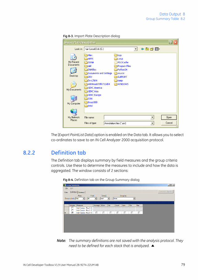
Data Output 8Group Summary Table 8.2
Fig 8-3. Import Plate Description dialog
The [Export PointList Data] option is enabled on the Data tab. It allows you to select co-ordinates to save to an IN Cell Analyzer 2000 acquisition protocol.
8.2.2 Definition tab The Definition tab displays summary by field measures and the group criteria controls. Use these to determine the measures to include and how the data is aggregated. The window consists of 2 sections:
Fig 8-4. Definition tab on the Group Summary dialog
Note: The summary definitions are not saved with the analysis protocol. They need to be defined for each stack that is analyzed.
IN Cell Developer Toolbox V1.9 User Manual 28-9274-22UM AB 79

8 Data Output8.2 Group Summary Table
1 The Group Criteria dropdown menus define the aggregation hierarchy, where the [Plate] dropdown provides the highest level of aggregation. You can chose between "All", "Well", "Row" or "Column".
The [Field] and [Time/Z] dropdowns offer two choices - "All" or "Each". If "All" is selected, all fields will be summarized in one value, whereas selecting "Each" will provide individual summaries for each field.
While the [Group by] dropdown lists all available measures, it is most useful if used to select a categorical measure to create sub-population summaries, like the output of a classifier.
2 The measures table area lists all available measures. To select a measure mark the checkbox in the [Include] column. For each measure the Average (mean), standard deviation (StDev), variance (Var), Count, Sum, minimal and maximal (Min, Max) values can be reported by checking the appropriate boxes.
Note: The Group Summary table can also be used to summarize cell tracking results. E.g. selecting [Time/Z]: "All" and [Group by]: "Label" allows reporting the sum and/or averages of step distances for all tracks.
On the Definition tab, the File menu the following options are enabled.
Fig 8-5. Group Summary - Data tab Edit menu options
The [Import Plate Description] option imports the Stack name which will display on the Summary tab.
Selecting the option opens the Import Plate Description dialog, where you can
80 IN Cell Developer Toolbox V1.9 User Manual 28-9274-22UM AB

Data Output 8Group Summary Table 8.2
select an XML file containing the annotation.
8.2.3 Summary tab The Summary tab displays the aggregate analysis data that matches the criteria selected on the Definition tab. Note that you can sort the table according to your needs by clicking on any column. By default, the Summary displays the data classified according to the criteria well, all fields, each time or z and no classification.
Fig 8-6. Summary tab on the Group Summary dialog
The table display has the following characteristics:
• The imported Plate ID appears in the table regardless of group criteria selected, and measures selected on the Definition tab.
• After sampling in Developer the Group Summary - Summary tab table data is formatted to display 11 decimal places and right aligned.
8.2.4 File Menu Options The File menu on this tab allows has the following options enabled:
Fig 8-7. File menu of the Summary tab in the Group Summary function
• The [Export XML Summary (Excel compatible)] menu item allows you to export the generated summary detail as an XML file in an Excel readable format. A Save dialog will open where you can specify a user-defined name.
IN Cell Developer Toolbox V1.9 User Manual 28-9274-22UM AB 81

8 Data Output8.2 Group Summary Table
This file can be viewed as an Excel spreadsheet and contains only the results statistical measures. This option requires that you have Microsoft Office Excel 2003 installed to read the file.
Note: The exported file contains only the parent information even when selected when displaying child info. Only the summary data will be saved as Excel file. This will aid in exporting the summary table to spot fire.
• The [Export Excel Summary] menu item allows you to save the group summary results as an Excel file The data is saved in the location chosen with the file name as entered. A Save dialog will open where you can specify a user-defined name.
• The [Import Plate Description] option imports the Stack name which will display on the Summary tab.
Selecting the option opens the Import Plate Description dialog, where you can select an XML file containing the annotation.
8.2.5 Summary Tab Edit Menu The [Copy] menu item allows you to copy data from table to the clipboard, Excel spreadsheet, or text editor.
1 Use the Edit>Copy menu option, highlight and use the right click on the mouse, or use the [CTRL + C] shortcut key to copy the selected data. The following are options to copying data from the Summary tab:
IMPORTANT The paste option does not flag duplicates and will overwrite any text already in a cell.
copy a cell copy multiple cells Highlight 1 or more cells & copy
copy t entire rowcopy multiple rows Highlight 1 or more rows & copy
copy column copy multiple columns Highlight 1 or more columns & copy
copy entire table Highlight entire table & copy
82 IN Cell Developer Toolbox V1.9 User Manual 28-9274-22UM AB

Data Output 8Group Summary Table 8.2
2 Open an Excel or Word document, and select the [Paste] option from the right click context menu OR use the [CTRL + V] shortcut key to paste the copied data.
8.2.6 Connect to Spotfire DecisionSite The button is enabled once the user clicks on Summary tab. You can launch Spotfire and import the current summary data for further analysis.
8.2.7 Save Group Summary with ProtocolIN Cell Investigator v1.6 allows the group summary data from Developer Toolbox to be exported to Excel as an option on the Protocol Wizard>Data Management window. When selected, the output file will be passed on to group summary application after the assay is run. The Excel file will saved in the same location as the Image stack file with the context, <Protocol name + datetime stamp.xls>.
Fig 8-8. Data Management window of protocol wizard
Note: The measures to save should have been selected on the Group Summary Definition tab prior to saving the protocol..
IN Cell Developer Toolbox V1.9 User Manual 28-9274-22UM AB 83

8 Data Output8.2 Group Summary Table
84 IN Cell Developer Toolbox V1.9 User Manual 28-9274-22UM AB

Outline Display Options (v 1.7) 9
9 Outline Display Options (v 1.7)
The Outline Display Options feature allows for the addition of target labels and target outlines to your images. Click the Outline Display Options icon, , on the Table toolbar. The Outline Display Options dialog displays.
Fig 9-1. Outline Display Options dialog
1 In the [Color Schema] option, select a label from the drop-down list. The possible options are:
• Target Based
• New Threshold (if defined)
• New Linear Discriminant (if defined)
• New Decision Tree (if defined)
2 Mark the checkboxes to enable:
• [Display target label (if available)] -object labels will display on the image
• [Display target outline only] -objects will appear outlined
IN Cell Developer Toolbox V1.9 User Manual 28-9274-22UM AB 85

9 Outline Display Options (v 1.7)
3 After making your selections, click [Apply]. Examples of labeled and outlines objects are shown below.
Fig 9-2. Object showing Target label and Outline (left). Outline of nucleus and cell (right)
86 IN Cell Developer Toolbox V1.9 User Manual 28-9274-22UM AB

Context Modules 10Version 1.7 Updates 10.1
10 Context Modules
Fig 10-1. List of Context Modules
10.1 Version 1.7 Updates The Nuclear Translocation and Myotube Formation context modules were updated as described below:
• Nuclear Translocation - quantifies the cytoplasm-to-nucleus or nucleus-to-cytoplasm translocation of GFP-labeled target molecules by analyzing an image stack acquired by the IN Cell Analyzer 1000.
• Myotube Formation - image-based analysis of the formation of myotubes by analyzing an image stack acquired by the IN Cell Analyzer 1000.
In addition, the Cell Viability context module was added:
• Cell viability - analysis of cells simultaneously stained with a nuclear dye (e.g. Hoechst), a cell viability marker (such as esterase substrate Calcein AM), and a marker for non-viable cells (such as the membrane-impermeable DNA dye Propidium Iodide).
The cell viability context module allows you to classify cells into following
IN Cell Developer Toolbox V1.9 User Manual 28-9274-22UM AB 87
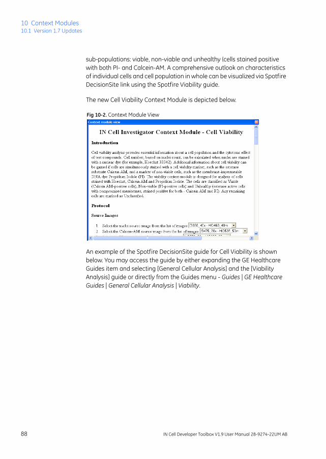
10 Context Modules10.1 Version 1.7 Updates
sub-populations: viable, non-viable and unhealthy (cells stained positive with both PI- and Calcein-AM. A comprehensive outlook on characteristics of individual cells and cell population in whole can be visualized via Spotfire DecisionSite link using the Spotfire Viability guide.
The new Cell Viability Context Module is depicted below.
Fig 10-2. Context Module View
An example of the Spotfire DecisionSite guide for Cell Viability is shown below. You may access the guide by either expanding the GE Healthcare Guides item and selecting [General Cellular Analysis] and the [Viability Analysis] guide or directly from the Guides menu - Guides | GE Healthcare Guides | General Cellular Analysis | Viability.
88 IN Cell Developer Toolbox V1.9 User Manual 28-9274-22UM AB

Context Modules 10Version 1.8 Updates 10.2
Fig 10-3. Cell Viability Guide
Note: In order to download the Guide, you must be a registered Spotfire user and connected to the internet. Please refer to Chapter 2, Visualizing Results with Spotfire DecisionSite and the IN Cell Investigator Installation Guide on connecting to the GE Healthcare Spotfire server.
10.2 Version 1.8 Updates For release v1.8, the Angiogenesis Context Module was added:
10.2.1 Angiogenesis Angiogenesis, the process of new blood vessel formation, plays a crucial role in many physiological and pathological events. The understanding of mechanisms of angiogenesis, as well as screening for pro- and anti-angiogenic compounds, are important therapeutic goals.
The Angiogenesis context module is designed to analyze the angiogenesis assay, performed on fibrin matrix (as described in the ‘Example image stack - Assay set up’ document, which can be accessed through the shortcut within the context module) with post-fixing and staining with fluorescent cytoplasmic and nuclear dyes.
Prior to analysis using the Angiogenesis context module, an extended focus transformation protocol (Chapter 2, Section 2.1 of this manual) should be applied to the acquired 3-D (z-series) image stack. The resulting 2-D projection
IN Cell Developer Toolbox V1.9 User Manual 28-9274-22UM AB 89

10 Context Modules10.3 Version 1.9 Updates
composite image stack can be then analyzed with Angiogenesis Context Module.
1 Selecting Angiogenesis Context Module (GEHC. CMAngiogenesis,xcm) from the list of Context Modules
Fig 10-4. Angiogenesis Context Module
10.3 Version 1.9 UpdatesFor release v1.9, two new Context Modules have been added:
• Early Endosomal Markers
• Neurite Outgrowth
90 IN Cell Developer Toolbox V1.9 User Manual 28-9274-22UM AB

Context Modules 10Version 1.9 Updates 10.3
10.3.1 Early Endosomal Markers The Early Endosomal markers context module is designed for analysis of endosomal trafficking in the images of cells with fluorescently tagged endosomal marker and a fluorescent nuclear stain (e.g. Hoechst). The context module reports cell-by-cell results as well as population based data to characterise redistribution of proteins from endosomes to cytosol via measures describing granularity in cells. These data can be further visualised in Spotfire DecisionSite using GE Healthcare Early Endosomal Markers analysis Spotfire guide.
An example assay set up and reported measures description documents can be accessed via the shortcut within the Context module's interface.
1 Selecting Early Endosomal Markers Context Module (GEHC. CM.Early.Endosomal.Markers,xcm) from the list of Context Modules
IN Cell Developer Toolbox V1.9 User Manual 28-9274-22UM AB 91
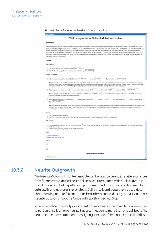
10 Context Modules10.3 Version 1.9 Updates
Fig 10-5. Early Endosomal Markers Context Module
10.3.2 Neurite Outgrowth The Neurite Outgrowth context module can be used to analyze neurite extensions from fluorescently labeled neuronal cells, counterstained with nuclear dye. It is useful for automated high-throughput assessment of factors affecting neurite outgrowth and neuronal morphology. Cell-by-cell, and population-based data, characterizing neurite formation, can be further visualized using the GE Healthcare Neurite Outgrowth Spotfire Guide with Spotfire DecisionSite.
In cell-by-cell neurite analysis, different approaches can be taken to relate neurites to particular cells when a neurite has a connection to more than one cell body. The neurite can either count it once, assigning it to one of the connected cell bodies
92 IN Cell Developer Toolbox V1.9 User Manual 28-9274-22UM AB

Context Modules 10Version 1.9 Updates 10.3
(without neurites partitioning) or it can be divided between the adjacent to it cell bodies (with neurites partitioning). Both analysis approaches are available from the Neurite Outgrowth context module.
Fig 10-6. Neurite OutgrowthContext Module
IN Cell Developer Toolbox V1.9 User Manual 28-9274-22UM AB 93

10 Context Modules10.3 Version 1.9 Updates
Fig 10-7. Samples of the A) Neurite Outgrowth (with Neurite Partitioning) and B) Neurite Outgrowth (without Neurite Partitioning) Context Modules.
A
94 IN Cell Developer Toolbox V1.9 User Manual 28-9274-22UM AB

Context Modules 10Version 1.9 Updates 10.3
Fig 10-8. Fig Y. (A) Neurite outgrowth in mouse renoblastoma Neuro-2a cells. Neuronal cells are labeled with FITC (using anti-neurofilament 200 kD subunit (NF200) primary antibody).* (B) Analysis with Neurite Outgrowth Context Module (without neurite partitioning). Nuclei (yellow), cells (red) and neurites (green) outlines. (C) Application of morphological measurements to neurites. * The 10x magnification images were acquired on the IN Cell Analyzer 1000.
B
IN Cell Developer Toolbox V1.9 User Manual 28-9274-22UM AB 95

10 Context Modules10.3 Version 1.9 Updates
96 IN Cell Developer Toolbox V1.9 User Manual 28-9274-22UM AB

Additional Features 11Version 1.7 Enhancements 11.1
11 Additional Features
11.1 Version 1.7 Enhancements A number of performance and data management features were added inVersion 1.7.
11.1.1 Multi-processor Support IN Cell Developer Toolbox benefits from the high performance of multi-core CPU systems in that the increased computing speed allows the analyzing of two blocks at one time on a computer with two CPU cores, or four blocks on a computer with four CPU core.
Note: Multiple analysis engines are automatically initialized at the beginning of an analysis. A slight delay at the start of an analysis may be experienced if no analysis engine is currently available.
The standard license for IN Cell Developer Toolbox 1.7 will enable the software to run on up to four cores in parallel. The installation wizard will detect systems that can support multi-processors and ask you to enable this feature to allow the ability to utilize the increased computing power.
IN Cell Developer Toolbox configured with multi-processor capabilities displays the [Analyzer Coordinator] icon, , on the taskbar. Not only is this an indicator of the resources available, it is also a valuable tool in assessing system usage.
Hovering the mouse over the icon displays the number of CPU cores currently available. Double-clicking on the icon will open the Analyzer Coordinator window, allowing you to diagnosis and/or verify the CPU usage of your IN Cell Developer Toolbox installation.
IN Cell Developer Toolbox V1.9 User Manual 28-9274-22UM AB 97

11 Additional Features11.1 Version 1.7 Enhancements
Fig 11-1. Analyzer Coordinator window showing use of 4 CPUs
11.1.2 Memory Management Improvements & New File Format
In order to deal more efficiently with the ever increasing size of image stacks generated by high content experiments, the memory management of the Investigator software has been significantly improved in this release.
Currently, IN Cell Investigator 1.3 supports image stacks with 384 wells by 70 fields and 3 colors. Actual memory consumption not only depends on the number of images within the stack (channels, fields, time points and z-planes) but also on the protocol definition, the number of objects detected, and the number of measures applied. Therefore, this 384 well by 70 field and 3 color stack size verification cannot be considered absolute.
A new analysis result file type, LG3, has been added to IN Cell Investigator. By default, LG3 is a zip file containing the analysis results for each field of view. Investigator no longer produces LG2 files, though previously created LG2 files can be imported and read by this version of IN Cell Investigator.
To support this new large image stack format, the following features and modifications have been added to IN Cell Investigator 1.3:
1 A local hard disk with available free-space of 20 GB is recommended as cache.
2 LG3 file type has replaced LG2 file type in the user interface.
3 When viewing analysis results, the data table may display only partial target data due to the availability of memory. For details on how to navigate the data table, refer to Section 11.1.3 Navigating Data Tables
98 IN Cell Developer Toolbox V1.9 User Manual 28-9274-22UM AB

Additional Features 11Version 1.7 Enhancements 11.1
11.1.3 Navigating Data Tables Tied to the introduction of the new memory management system in IN Cell Investigator 1.3, a new data file format, LG3, has been introduced (for more information, refer to Chapter 11 Additional Features).
1 When reviewing analysis results from large data sets, the data table may display only partial target (cell by cell) data depending on the available of memory. To navigate through the data set the following options are available in Developer Toolbox and Analysis Workstation:
2 When opening large datasets that exceed the available memory, the LG3 Options utility will become available. Access the Options dialog from either the View > LG3 options menu item or by clicking the green button located to the top left of the data table. LG3 option button has 2 states: full green ) indicates data from all fields are in target table; half green ( ) indicates data from some fields are in target table.
Starting from the field summary table
select one field, the target/cell data for that field will be displayed in the target table
Starting from the image stack view
select one field, the target/cell data for that field will be displayed in the target table
Using the LG3 option dialog
select any of the fields and click OK, the target/cell data for those fields will be displayed in the target table
IN Cell Developer Toolbox V1.9 User Manual 28-9274-22UM AB 99
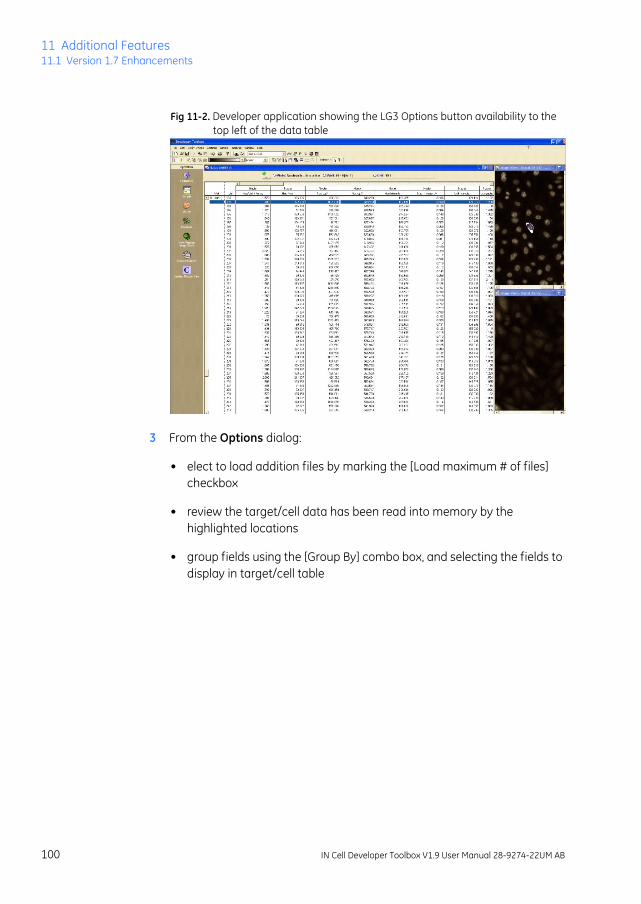
11 Additional Features11.1 Version 1.7 Enhancements
Fig 11-2. Developer application showing the LG3 Options button availability to the top left of the data table
3 From the Options dialog:
• elect to load addition files by marking the [Load maximum # of files] checkbox
• review the target/cell data has been read into memory by the highlighted locations
• group fields using the [Group By] combo box, and selecting the fields to display in target/cell table
100 IN Cell Developer Toolbox V1.9 User Manual 28-9274-22UM AB
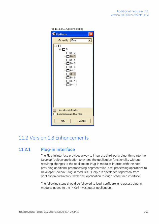
Additional Features 11Version 1.8 Enhancements 11.2
Fig 11-3. LG3 Options dialog
11.2 Version 1.8 Enhancements
11.2.1 Plug-in Interface The Plug-in interface provides a way to integrate third-party algorithms into the Develop Toolbox application to extend the application functionality without requiring changes to the application. Plug-in modules interact with the host providing additional preprocessing, segmentation, post processing operations to Developer Toolbox. Plug-in modules usually are developed separately from application and interact with host application through predefined interface.
The following steps should be followed to load, configure, and access plug-in modules added to the IN Cell Investigator application.
IN Cell Developer Toolbox V1.9 User Manual 28-9274-22UM AB 101

11 Additional Features11.2 Version 1.8 Enhancements
11.2.1.1 Load plugins The plug-in DLL files must be placed in the Developer Toolbox application folder, and then enabled within the Developer Toolbox application itself.
1 Plug-in modules are added by placing a DLL file in the PLUGIN directory of the Developer Toolbox application:. . Default location of PLUGIN directory is
C:\Program Files\GE Healthcare\IN Cell Developer Toolbox v1.8\PLUGIN.
The DLLs are recognized upon start-up of the application and are loaded. Once loaded, these methods will be listed in the Protocol Explorer Component Overview under their respective operations groups
If one or more DLL's in the plug-in folder under IN Cell Investigator are not of the correct form, the following message displays during start up:
Opening application session log provides information on the success or failure of the plugin load process.
Navigating to and opening the error.log file in the PLUGIN folder provides information on the success or failure of the plugin load process.
102 IN Cell Developer Toolbox V1.9 User Manual 28-9274-22UM AB
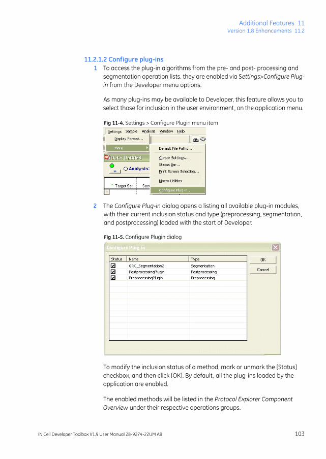
Additional Features 11Version 1.8 Enhancements 11.2
11.2.1.2 Configure plug-ins 1 To access the plug-in algorithms from the pre- and post- processing and
segmentation operation lists, they are enabled via Settings>Configure Plug-in from the Developer menu options.
As many plug-ins may be available to Developer, this feature allows you to select those for inclusion in the user environment, on the application menu.
Fig 11-4. Settings > Configure Plugin menu item
2 The Configure Plug-in dialog opens a listing all available plug-in modules, with their current inclusion status and type (preprocessing, segmentation, and postprocessing) loaded with the start of Developer.
Fig 11-5. Configure Plugin dialog
To modify the inclusion status of a method, mark or unmark the [Status] checkbox, and then click [OK]. By default, all the plug-ins loaded by the application are enabled.
The enabled methods will be listed in the Protocol Explorer Component Overview under their respective operations groups.
IN Cell Developer Toolbox V1.9 User Manual 28-9274-22UM AB 103

11 Additional Features11.2 Version 1.8 Enhancements
3 To confirm the load and/or access a plug-in module, right-click on either:
• Preprocessing>Insert as First Preprocess
• Segmentation>Change Segmentation
• Postprocessing>Insert as First Postprocess
and select the plug-in method from the displayed list.
Fig 11-6. Example of a plugin enabled on the Preprocess listing
Note: The plug-in modules will be added to the end (bottom) of the list .
The Component Settings for the method display, if appropriate. Define the parameters as necessary.
Fig 11-7. Example of a plug-in Component Settings panel
104 IN Cell Developer Toolbox V1.9 User Manual 28-9274-22UM AB

Additional Features 11Version 1.9 Enhancements 11.3
11.2.1.3 Configure plug-in directory IN Cell Developer Toolbox will scan for plug-ins in a specified folder named "PLUGIN" under the application folder by default. However, the location of plug-in folder can be changed to a user specified path.
In order to change default location, open the Settings menu from the Developer Toolbox Main menu, and select More>Default File Paths.
You will find "Default File Path Settings" dialog. Change path for plug-in under title "Plugin folder:"
Fig 11-8. Default File Path Settings dialog
11.3 Version 1.9 Enhancements
11.3.1 Analyzing Image Stacks Other than IN Cell Analyzer1000/2000 Note: The [Other format] option is available only if there is a valid IN Cell Translator
v2.0license on the machine on which IN Cell Investigator is running.
The Developer Toolbox v1.9 application is capable of analyzing data acquired on instruments other than the IN Cell Analyyzer 1000 and/or 2000.
IN Cell Developer Toolbox V1.9 User Manual 28-9274-22UM AB 105

11 Additional Features11.3 Version 1.9 Enhancements
A converted stack will be named with the original name appended with .xdce. The user will be provided an indicator that the file has been converted, while allowing him to see the original stack name. Any analysis data will be stored with the converted image stack file.
Access the Retrieve Image Stack dialog by either:
• Opening Images menu > [Retrieve …]
• the View/Analyze Image Stack icon located on the shortcut Operations bar
Use the Retrieve Image Stack file dialog to locate and select the image stack file. The IN Cell Developer Toolbox application supports generic stacks (.xgis), IN Cell Analyzer 1000 stacks (.dce, .xdce, .xml), and IN Cell Analyzer 3000 stacks (.run). Select this icon to open an image stack (*.dce,*.xdce, *.run files). A new File 'Other Format is available for files of type .txt, .dib, .htd, and .mac.
In Batch Analysis Mode, select Analysis-> Batch Analysis Manager, and open the Add Image Stacks to Batch Queue dialog. Four new check boxes (.txt, .dib, .htd, .mac), have been added under the Scanning Options group to allow access when a valid IN Cell Translator license is available on the application computer.
The image stack will be stored in the batch queue file as .txt, .dib, .htd, .mac files. When application performs analysis these stacks are converted into .xdce format.
106 IN Cell Developer Toolbox V1.9 User Manual 28-9274-22UM AB

Additional Features 11Version 1.9 Enhancements 11.3
Fig 11-9. Add Image Stacks to Batch Queue dialog
11.3.2 Interfacing with IN Cell Miner HCM
IN Cell Developer Toolbox provides an interface to the IN Cell Miner HCM application, to store analysis data collected from image analysis. Image stacks (*.xdce) and analysis results (*.LG2/*.LG3) can be:
• Exported from Developer Toolbox to store large volumes of analysis data
• import ed from IN Cell Miner for re-analysis and upstream processing by Developer Toolbox
11.3.2.1. Exporting Analysis Data To IN Cell Miner Analysis data can be saved to the IN Cell Miner HCM directly from the Protocol wizard.
1 From the New or Edit Protocol wizards, mark the [Export to IN Cell Miner HCM] checkbox on the Data Management dialog.
WARNING! This feature requires that a licensed version of IN Cell Miner HCM is available. and the user has a valid IN Cell Miner HCM login.
IN Cell Developer Toolbox V1.9 User Manual 28-9274-22UM AB 107

11 Additional Features11.3 Version 1.9 Enhancements
Fig 11-10. Data Management dialog option to upload to data to IN Cell Miner HCM
When the protocol is used, the IN Cell Miner Login dialog displays. You can:
• Provide your IN Cell Miner logon credentials and and click [OK] to initiate an IN Cell Miner login session.
• Select 'Cancel', to abort the login process and proceed without logging into Miner.
Fig 11-11. Logon dialog from IN Cell Investigator to IN Cell Miner HCM
2 Upon successful login to IN Cell Miner, the Browse Projects dialog opens, displaying the project hierarchy to which you have read/write privileges.
108 IN Cell Developer Toolbox V1.9 User Manual 28-9274-22UM AB

Additional Features 11Version 1.9 Enhancements 11.3
Fig 11-12. IN Cell Miner HCM - Browse Projects dialog
3 Navigate the project tree to the plate and assigned image stack to which to export the analysis results.
Note: Any analysis data associated with the stack will display.
If the image stack has not yet been exported to IN Cell Miner, highlight the plate and open the context menu. Selelct [Add Image Stack]. The currently open image stack will be exported to IN Cell Miner HCM with the generated anallysis results.
Fig 11-13. IN Cell Miner HCM - Browse Projects dialog showing the Add Image Stack option.
IN Cell Developer Toolbox V1.9 User Manual 28-9274-22UM AB 109
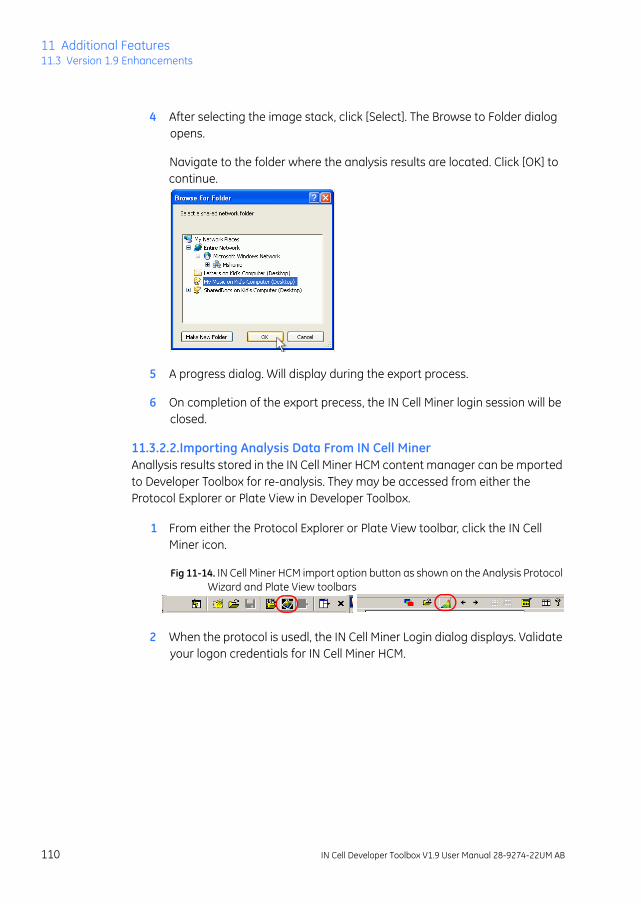
11 Additional Features11.3 Version 1.9 Enhancements
4 After selecting the image stack, click [Select]. The Browse to Folder dialog opens.
Navigate to the folder where the analysis results are located. Click [OK] to continue.
5 A progress dialog. Will display during the export process.
6 On completion of the export precess, the IN Cell Miner login session will be closed.
11.3.2.2.Importing Analysis Data From IN Cell MinerAnallysis results stored in the IN Cell Miner HCM content manager can be mported to Developer Toolbox for re-analysis. They may be accessed from either the Protocol Explorer or Plate View in Developer Toolbox.
1 From either the Protocol Explorer or Plate View toolbar, click the IN Cell Miner icon.
Fig 11-14. IN Cell Miner HCM import option button as shown on the Analysis Protocol Wizard and Plate View toolbars
2 When the protocol is usedl, the IN Cell Miner Login dialog displays. Validate your logon credentials for IN Cell Miner HCM.
110 IN Cell Developer Toolbox V1.9 User Manual 28-9274-22UM AB

Additional Features 11Version 1.9 Enhancements 11.3
Fig 11-15. Logon validation window from IN Cell Investigator
3 Upon successful login to IN Cell Miner, the Browse Projects dialog opens, displaying the project hierarchy to which you have read/write privileges.
Navigate the project tree to the Image stack to be imported and highlight the Image stack to select.
Fig 11-16. IN Cell Miner HCM - Browse Projects dialog
4 After selecting the image stack, click [Select].
5 A progress dialog. Will display during the import process. A browse for folder dialog opens through which user has to select the folder into which to download the Image stack from miner.
6 Once data is imported to IN Cell Investigator he IN Cell Miner login session will be closed. The new stack will be automatically opened in the Image viewer of developer.
IN Cell Developer Toolbox V1.9 User Manual 28-9274-22UM AB 111

11 Additional Features11.3 Version 1.9 Enhancements
112 IN Cell Developer Toolbox V1.9 User Manual 28-9274-22UM AB

Rehosting your E-License 12
12 Rehosting your E-License
The Investigator software is licensed to run on one specific computer identified by the physical address of its Ethernet adapter (also referred to as MAC address, a unique identifier of your PC). If you want to use the software on a different PC (e.g., one with higher specifications to benefit from the new multi-processing feature), you will need to move the license to that PC (or purchase an additional license).
Moving an E-license from one computer to another is called rehosting. If you need to rehost a license, you should contact Technical Support/Customer Service (see the last page.). Customer service will then send a Rehost Request form to you to fill out, sign and send back. Once that is done and the reason for the rehost is valid, the representative will rehost your license.
Please refer to the IN Cell Investigator Installation Guide for details on how to install your software and take receipt of your license.
IN Cell Developer Toolbox V1.9 User Manual 28-9274-22UM AB 113

12 Rehosting your E-License
114 IN Cell Developer Toolbox V1.9 User Manual 28-9274-22UM AB


For local office contact information, visit:
www.gelifesciences.com/contact
GE Healthcare UK Ltd Amersham Place, Little Chalfont, Buckinghamshire, HP7 9NA, UK
www.gelifesciences.com
GE, imagination at work and GE monogram are trademarks of General Electric Company.
The IN Cell Analyzer system and the In Cell Investigator software are sold under use license from Cellomics Inc. under US patent numbers US 5989835, 6365367, 6416959, 6573039, 6620591, 6671624, 6716588, 6727071, 6759206, 6875578, 6902883, 6917884, 6970789, 6986993, 7060445, 7085765, 7117098, 7160687, 7235373, 7476510 ; Canadian patent numbers CA 2282658, 2328194, 2362117, 2381344; Australian patent number AU 730100; European patent numbers EP 0983498, 1095277, 1155304, 1203214, 1348124, 1368689; Japanese patent numbers JP 3466568, 3576491, 3683591, 4011936 and equivalent patents and patent applications in other countries
All third party trademarks are the property of their respective owners.
© 2004–2010 General Electric Company - All rights reserved.Previously published July 2008.
Notice to purchaserThe IN Cell Analyzer system is for research purposes only. It is not approved for diagnosis of disease in humans or animals.
The IN Cell Investigator is sold for use in a variety of research applications. The purchase of this product does not include a license under any patent or intellectual property to use IN Cell Investigator in any particular application. It is strongly recommended that the purchaser consider the need for a license to the intellectual property of others that may cover an intended use.
By using this software, the purchaser acknowledges the above referenced license constraints and accepts responsibility for all patents that may apply in using IN Cell Investigator in any particular application.
License agreementEnd-User is required to accept the end-user license terms and conditions set forth on www.gehealthcare.com/investigator/license before installing and using the GE Healthcare software
All goods and services are sold subject to the terms and conditions of sale of the company within GE Healthcare which supplies them. A copy of these terms and conditions is available on request. Contact your local GE Healthcare representative for the most current information.
GE Healthcare Bio-Sciences AB Björkgatan 30 751 84, Uppsala, Sweden
GE Healthcare Bio-Sciences Corp800 Centennial Avenue, P.O. Box 1327, Piscataway, NJ 08855-1327, USA
GE Healthcare Europe GmbHMunzinger Strasse 5, D-79111 Freiburg, Germany
GE Healthcare Japan CorporationSanken Bldg. 3-25-1, Hyakunincho, Shinjuku-ku, Tokyo 169-0073, Japan
28-9274-22UM AB 05/2010
imagination at work