Inflation-linked public debt in emerging economies I

Patricia Gomez-Gonzalez

Fordham University

Abstract

This study reports a set of stylized facts about inflation-linked (IL) public

debt in emerging economies. On average, emerging economies issue 23% of

their local currency (LC) public debt linked to inflation. IL debt issuance

is countercyclical, increases in periods of nominal exchange rate deprecia-

tions, and substitutes foreign currency (FC) and non-indexed local currency

debt. A two-sector small-open economy model of public debt composition

can deliver the business-cycle properties of IL debt and shows that, during

crises, amid nominal exchange rate depreciations, IL debt becomes cheaper

to issue. The study finds evidence of IL rates decreasing in about half of the

most recent crises in emerging economies. Finally, the study compares IL

rates to FC and LC rates and concludes that, for some countries, IL rates

are below LC rates, even after accounting for expected inflation.

IThis project benefited from the support of Fordham University’s Office of ResearchFaculty Research Grant and Manuscript and Book Publication Award (MBPA). I thankJohanna Francis, Subha Mani, Susana Martins, Sophie Mitra, Diego Perez, Jesse Schreger,and attendees to presentations at the XXI Encuentro de Economıa Espanola, the NorthAmerican Econometric Society 2018 Summer Meeting, and the University at Albany forthoughtful comments and suggestions. Nicholas Rizzo provided excellent research assis-tance and Luis Molina in the Banco de Espana assisted with interest rate data collection.

1Fordham University. 113 W 60th Street, Room 924. New York,NY 10023. USA. Email address: pgomezgonzalez@fordham.edu and URL:http://faculty.fordham.edu/pgomezgonzalez

Preprint submitted to Journal of International Money and Finance January 28, 2019

Keywords: Public debt, Inflation-linked debt, Foreign currency debt

JEL: F34, F41, H63

1. Introduction

Emerging economies issue a sizeable share of their public debt linked

to inflation. Since 2004, in the study’s sample, emerging economies have

issued, on average, 23% of their local currency (LC) public debt linked to

inflation and emerging economies’ issuance of this type of debt has increased,

on average, by five times since 1995.

Furthermore, for almost half the countries in the study’s sample, inflation-

linked (IL) rates are below LC rates, even after accounting for expected future

inflation rates. For these countries, IL rates are between 1.2 and 5 percentage

points lower than LC rates.

Despite the quantitative importance of this type of bond and the policy

implications regarding IL rates in comparison to LC rates for some coun-

tries in the sample, relatively little is known about IL debt’s business cycle

properties. This paper aims to fill this gap.

The data shows evidence of the IL debt issuance being countercyclical,

increasing when the domestic currency is weaker, and substituting FC debt

and non-indexed LC debt inssuance.

Previous work has studied IL debt vis-a-vis non-indexed LC debt (Bohn

(1988), Bohn (1990), Calvo and Guidotti (1990), Diaz-Gimenez et al. (2008),

Alfaro and Kanczuk (2010), Sunder-Plassmann (2017)). This study comple-

ments this literature by examining IL debt vis-a-vis FC debt and by offering

a description of the IL debt issuance’s business cycle properties.

2

To this end, the study presents a two-sector small-open economy model

of public debt composition, where a government, who needs to finance an

exogenous level of government spending, raises taxes, issues IL and FC debt

in foreign debt markets, and commits to repay both types of securities.

The model abstracts from sovereign default because there is no evidence

of differential sovereign risk associated to LC and FC debt (Du and Schreger

(2016), Jeanneret and Souissi (2016)). The rationale for contemplating dif-

ferential LC/FC sovereign risk in the first place is that, LC debt burden

can be inflated-away, making outright default unnecessary for a country that

wishes to renege on its debt. However, because IL debt is indexed, it cannot

be inflated-away, implying that, from a sovereign risk perspective, it is like

FC debt (Fleckenstein et al. (2014)).

Aside from outright default, underreporting inflation data defrauds hold-

ers of IL debt, whose returns fall short of protecting against actual realized

inflation. With the exception of Argentina, the credibility of inflation statis-

tics, for the countries in the study’s sample, is not a source of concern2 and,

hence, the model abstracts from inflation statistics misreporting.

The key result of the model is that during an economic crisis, when the

economy endures a nominal exchange rate depreciation, IL debt becomes

cheaper to issue, making the government move away from FC debt and in-

crease its IL debt issuance. The reason is that, if bad shocks are short-lived,

a depreciation now implies an expected appreciation in the near future, low-

2See, for example, The Economist’s argument to stop reporting official in-

flation statistics in 2014 (https://www.economist.com/leaders/2014/06/20/

dont-lie-to-me-argentina).

3

ering foreign investors’ required return to buy IL debt.

Under the purview of this model, the country substitutes FC debt for IL

debt because the latter becomes cheaper to issue during crises. To explore

whether the data supports this finding, the study examines the behavior

of IL rates around recent crises in emerging economies and finds that, in

approximately half of them, IL rates fell.

The rest of the paper is structured as follows. Section 2 presents the

stylized facts about IL debt issuance for a sample of emerging economies.

Section 3 lays out the baseline model. Section 4 presents the key result on

the substitution of FC debt for IL debt. Section 5 explores IL rates during

recent crises in emerging economies and investigates the role of expected

inflation and expected exchange variations in explaining the positive FC-IL

and LC-IL rate differentials. Section 6 concludes the study.

1.1. Literature Review

This study is related to several strands of the literature. First, it is related

to the literature on IL public debt and the references cited in the previous

subsection. These studies all examine IL public debt vis-a-vis non-indexed

LC debt in an environment where the government lacks commitment. In

such environment, the IL debt proves beneficial by acting as a commitment

device for the government, lowering the cost of borrowing. The drawback

of IL debt lies in the government’s inability to introduce state-contingency

through inflation.

Second, it is related to the vast literature on FC debt, which studies FC

debt vis-a-vis LC debt. The ’original sin’, or emerging economies’ inability

to borrow abroad in LC, gained considerable attention (Eichengreen et al.

4

(2005, 2007)). Recently, Du and Schreger (2016) notice an improvement in

this situation and Du et al. (2016) find greater improvements in this situa-

tion for countries with high monetary policy credibility. From a normative

perspective, Engel and Park (2017) and Ottonello and Perez (Forthcoming)

examine the optimal composition of LC and FC debt in an environment with

strategic default and/or strategic debasement through inflation. In this lit-

erature, FC debt acts as a commitment device for the government, lowering

the cost of borrowing. The drawback of FC debt, like IL debt in the previous

literature, lies in the government’s inability to introduce state-contingency

through inflation.

This study complements the two previous literatures by studying IL debt

vis-a-vis FC debt and describing IL debt’s business cycle properties.

Third, it is related to the literature on asset heterogeneity in public debt.

In addition to the FC/LC debt dychotomy and the references mentioned

above, the maturity composition of public debt obtained substantial atten-

tion (Arellano and Ramanarayanan (2012), Broner et al. (2013), Fernandez

and Martin (2015), Aguiar et al. (2016), Bocola and Dovis (2016)). This

study focuses on IL debt, relatively understudied in the literature on asset

heterogeneity in public debt.

Finally, from the modeling standpoint, to study the business cycle prop-

erties of IL debt, the paper uses a standard real business-cycle model with

two sectors of production similar to those in Mendoza (1995), Stockman and

Tesar (1995), Corsetti et al. (2008), and Schmitt-Grohe and Uribe (2018) to

name a few. The model in this study embeds a government, taxes, and two

types of bonds and is able to study the cyclical behavior of bond rates.

5

2. Stylized Facts

This section compiles a set of stylized facts about IL debt issuance for a

sample of emerging economies. Appendix A lists the countries in the sample

and the data sources.

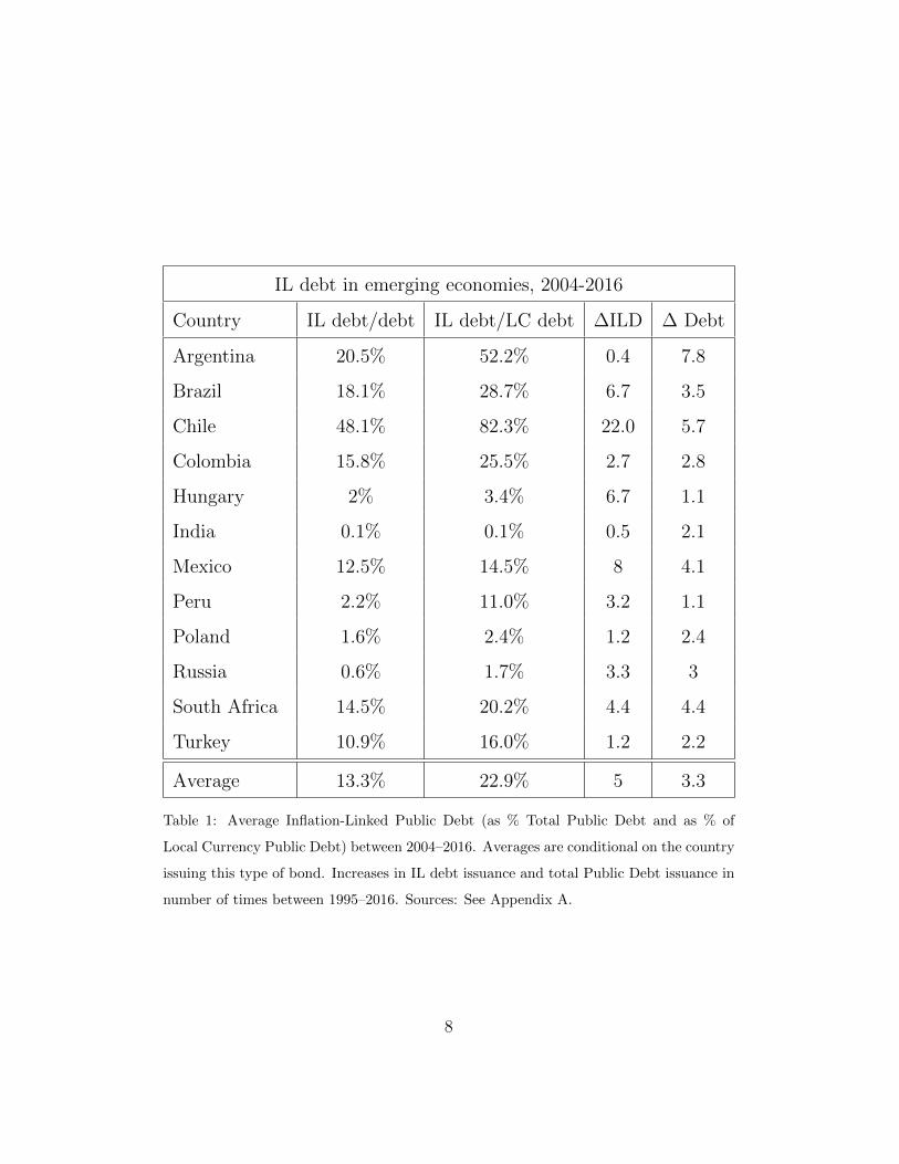
Fact 1: Emerging economies have issued, on average, 13% of their public

debt linked to inflation between 2004 and 2016. This represents 23% of their

LC debt.

Table 1 shows the share of IL debt over total debt (column 2) and the

share of IL debt over LC debt (column 3) between 2004 and 2016. The last

row shows the average IL debt issuance for the countries in the sample—

13.3% of total public debt and 22.9% of LC debt.

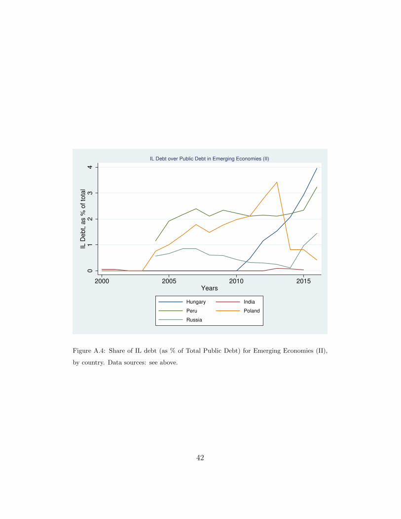
The table shows substantial heterogeneity across countries. Five countries

(i.e., Hungary, India, Peru, Poland, and Russia) issue less than 3% of their

total debt linked to inflation, while the remaining countries in the sample,

issue a more substantial share. Figures A.3 and A.4 in Appendix A plot the

entire time-series of IL debt over total debt for the two groups of countries

in the sample.

Columns 4 and 5 in table 1 show that, on average, IL debt has increased

fivefold since 1995, while public debt has, on average, only tripled. All coun-

tries, except Argentina, India, Poland, and Turkey, have increased their IL

debt issuance by more than their total public debt issuance.

Understanding the cross-section heterogeneity in table 1 or why some

emerging economies (e.g., Czech Republic, Indonesia, Malaysia or Thailand)

6

refrain from issuing this type of debt is outside the scope of this study3.

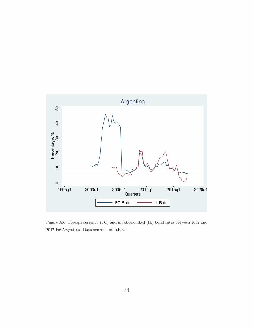
Fact 2: IL rates are below FC and LC rates.

IL rates are below FC rates and LC rates for most of the economies in the

sample and for most of the time period considered. See figures A.6 and A.7

in Appendix A for IL and FC rates and A.8 and A.9 in the same appendix

for IL and LC rates. There are some exceptions, but most of the countries

during most of the period under consideration exhibit a positive differential

between the FC and the IL rates and between the LC and the IL rates.

Table 2 shows the average IL rate (column 2), FC rate (column 3), and LC

rate (column 4). The last two rows report the cross-sectional average for each

of these rates and show that, in the cross-section, IL rates are 1.7 percentage

points lower than FC rates, when excluding Argentina’s 2001 default, and

4.8 percentage points lower than LC rates.

The degree to which expected inflation rates and expected exchange rate

variations can explain the differences in rates is explored in the last section

of the paper.

The remaining facts refer to the business cycle properties of IL debt.

For IL debt, I use issuance data between 1995 and 2016 deflated using the

GDP deflator. The remaining variables of interest are the following: real

GDP, FC and non-indexed LC debt deflated using the GDP deflator, the

nominal exchange rate defined as units of LC to buy 1 US dollar, real effective

3 Du et al. (2016) find that only countries with high monetary policy credibility can

afford issuing LC debt instead of FC debt. Insofar IL debt resembles FC debt, the high

IL debt economies should have low monetary policy credibility.

7

IL debt in emerging economies, 2004-2016

Country IL debt/debt IL debt/LC debt ∆ILD ∆ Debt

Argentina 20.5% 52.2% 0.4 7.8

Brazil 18.1% 28.7% 6.7 3.5

Chile 48.1% 82.3% 22.0 5.7

Colombia 15.8% 25.5% 2.7 2.8

Hungary 2% 3.4% 6.7 1.1

India 0.1% 0.1% 0.5 2.1

Mexico 12.5% 14.5% 8 4.1

Peru 2.2% 11.0% 3.2 1.1

Poland 1.6% 2.4% 1.2 2.4

Russia 0.6% 1.7% 3.3 3

South Africa 14.5% 20.2% 4.4 4.4

Turkey 10.9% 16.0% 1.2 2.2

Average 13.3% 22.9% 5 3.3

Table 1: Average Inflation-Linked Public Debt (as % Total Public Debt and as % of

Local Currency Public Debt) between 2004–2016. Averages are conditional on the country

issuing this type of bond. Increases in IL debt issuance and total Public Debt issuance in

number of times between 1995–2016. Sources: See Appendix A.

8

Interest rates on different debt instruments, 2002-2017

Country IL rate (rIL) FC rate (rFC) LC rate (rLC)

Argentina 10.1% 16.7% 23.3%

Brazil 6.3% 7.7% 13.9%

Chile 2.6% 4.9% 5.0%

Colombia 4.7% 6.7% 7.4%

Hungary - 4.8% 6.5%

India 5.6% 3.4% 7.9%

Mexico 3.7% 5.7% 7.4%

Peru 6.3% 6.5% 6.2%

Poland 2.5% 4.5% 5.3%

Russia 2.9% 6.9% 7.8%

South Africa 2.4% 5.6% 9.1%

Turkey 2.5% 7.3% 20.2%

Average 4.6% 6.9% 9.4%

Excluding Argentina 2001Q4-

2005Q2

4.6% 6.3% 9.4%

Table 2: Interest Rates on different Debt Instruments: IL, FC and LC debt.Time coverage

depends on country and instrument. See Appendix A for time coverage and sources.

9

exchange rates (REER) defined as the real exchange rate against the basket

of the country’s trading partners, and the GDP deflator and the consumer

price index (CPI) as measures of inflation. For data sources, see Appendix

A.

Table A.12 in Appendix A shows the results of Im et al. (2003) unit root

tests for panel data with heterogenous panels for the aforementioned vari-

ables. The conclusion of these tests is that we cannot reject the presence of

unit roots in all panels for all variables. Hence, to make the series stationary,

the stylized facts that follow use the first differences of log variables.

Stylized facts 3-6 refer to table 3, which reports fixed-effects regression

coefficient estimates of β for regressions of the form:

∆ILDi,t = αi + β∆xi,t + εit (1)

where ∆ILD = ln(ILDt)− ln(ILDt−1) denotes the log difference of IL debt

issuance, ∆x = ln(xt) − ln(xt−1) denotes the log differences of the different

variables of interest in column 1 of table 3, and αi denotes country fixed-

effects.

The β coefficient in specification (1) states how much does ∆ILD change,

for a given country, as ∆x varies over time. This is exactly the correlation of

interest. The change in ∆x across time can be due to common time shocks

to all countries, since specification (1) omits time fixed-effects.

Table 3 reports the β coefficient estimates in the sample with (column

2) and without Argentina (column 3). The reason to study a subsample

without Argentina is the lack of credibility of its official statics, which caused

10

investors to move away from this country’s IL debt4, making IL debt issuance

likely to be less related to the Argentinean business cycles. Furthermore, this

lack of credibility might explain the substantial decline, since 2004, in the

Argentinean share of public debt linked to inflation shown in table A.14 in

Appendix A.

Fact 3: When excluding Argentina from the sample, IL debt issuance is coun-

tercylical.

The coefficient on real GDP in table (3) shows that a 1% increase in real

GDP is associated with a 5.3% drop in the amount of IL debt issued, when

Argentina is excluded from the sample.

By including Argentina in the sample, the p-value of the regression in-

creases to 0.102, and hence barely non-significant at a 10% significance level.

However, it is hardly surprising that including Argentina in the sample causes

IL debt issuance to become unrelated to the country’s real GDP, since Ar-

gentina’s IL debt issuance was most likely related to the lack of demand from

investors, due to official inflation underreporting.

Fact 4: IL debt issuance substitutes FC and non-indexed LC debt issuance.

A 1% drop in FC debt issuance increases IL debt issuance by 0.2% and a

1% drop in non-indexed LC debt issuance increases IL debt issuance by 0.4%

(or 0.3% in the sample without Argentina).

The model in the next section focuses on the substitution of FC debt for

IL debt, since it is one of the study’s novel finding. Figure A.5 in Appendix

4The Financial Times reported in 2012 about this on ”Argentina: inflation-linked peso

bonds take a dive”. Financial Times. July 16, 2012.

11

Estimates of β coefficient in fixed-effects regressions of the form

∆ILDi,t = αi + β∆xi,t + εit

All Sample Excluding Argentina

GDP -3.537 -5.331∗

(2.85) (2.77)

FC debt -0.220∗∗ -0.19∗∗

(0.08) (0.06)

Nominal debt -0.406∗∗ -0.291∗

(0.18) (0.14)

Debt -0.167 0.05

(0.27) (0.23)

Exchange rate 1.411∗ 1.664∗

(0.78) (0.79)

REER -2.026 -2.232

(1.18) (1.24)

GDP Deflator 2.883 3.722

(2.05) (2.07)

CPI - 3.606∗

(1.96)

Table 3: Estimates of β coefficient in fixed-effects regressions of the form ∆ILDi,t =

αi + β∆xi,t + εit. Robust standard errors are in parantheses. Significance levels: ∗p <

0.1,∗∗ p < 0.05,∗∗∗ p < 0.01

12

A shows the shares of IL debt and FC debt (over total government debt)

between 2004 and 2016 for Chile, Hungary, Mexico, and Peru. Chile in the

first row is a particularly good example of the substitution of FC debt for IL

debt.

Fact 5: Emerging economies increase IL debt issuance when the nominal

exchange rate depreciates.

A 1% depreciation in the exchange rate increases IL debt issuance by 1.4%

and 1.7% in the sample without Argentina. The behavior of the exchange

rate is key to understand the substitution of FC debt for IL debt. The model

in the next section makes this clear.

Fact 6: Emerging economies increase IL debt issuance when inflation is

high.

The estimated coefficient for the CPI is evidence of this. Due to unavail-

ability of Argentinean inflation data, the estimate is only reported for the

sample without Argentina. A 1% increase in inflation is associated with a

3.6% increase in IL debt issuance.

This association could mask reverse-causality. When governments issue

more of their debt linked to inflation, eroding the real value of the total

debt stock requires a higher inflation rate. Thus, a non-independent Central

Bank would let inflation increase as a response to the government’s IL debt

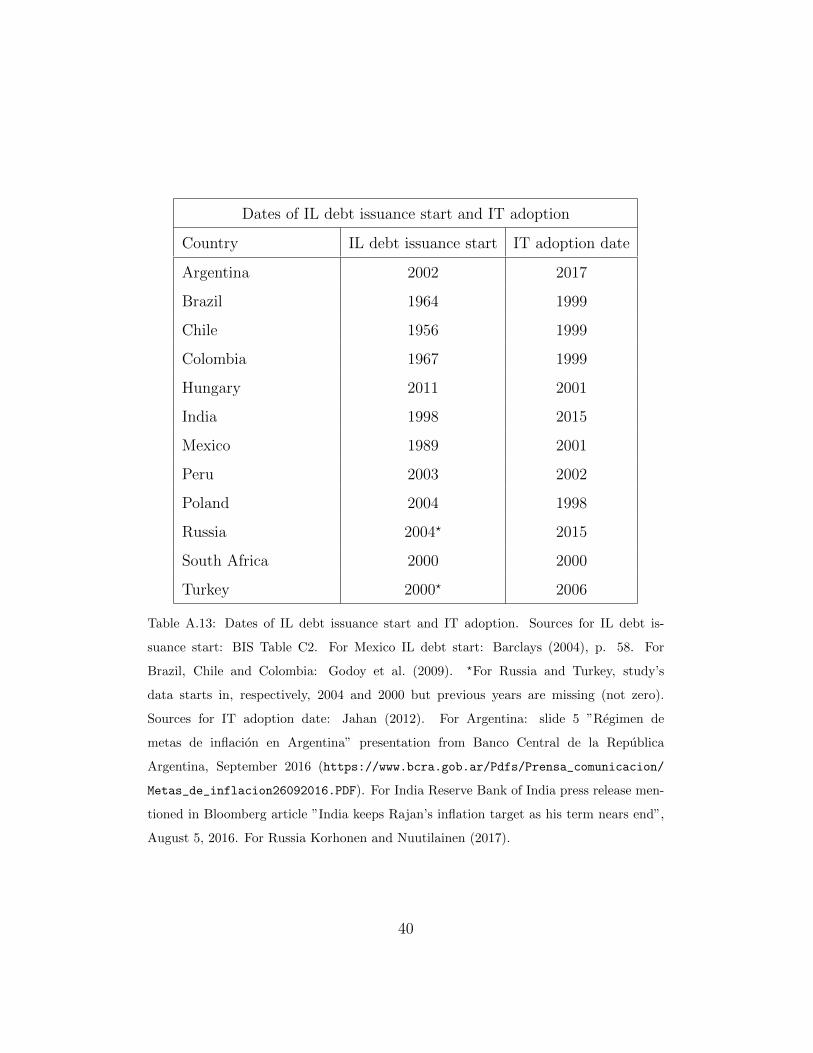
issuance. However, all countries in the study’s sample have inflation-targeting

(IT) Central Banks. See table A.13 in Appendix A for the dates of IT

adoption.

Table 4 show the relationship between inflation and IL debt issuance for

13

Estimates of β coefficient in fixed-effects regressions of the form

∆ILDi,t = αi + β∆xi,t + εit

After IT adoption After IT adoption excl. Argentina

GDP Deflator - 3.415

- (1.93)

CPI - 1.156

- (3.39)

Table 4: Estimates of β coefficient in fixed-effects regressions of the form ∆ILDi,t =

αi + β∆xi,t + εit, including only IT years. Robust standard errors are in parantheses.

Significance levels: ∗p < 0.1,∗∗ p < 0.05,∗∗∗ p < 0.01

the subsample in which countries are inflation-targeters5. The point esti-

mates remain positive, but lose significance.

Because the association between inflation and IL debt is absent for the

IT years and all countries in the study’s sample have IT Central Banks, the

model in the next section concentrates on the previous stylized facts. Even

if IT Central Banks had the incentive to miss their target and let inflation

increase, this would be most relevant for the IL/LC dychotomy and less for

the IL/FC dychotomy. Indeed, an increase in inflation would depreciate the

currency, making both IL and FC debt comparable.

To sum-up, the next section studies facts 3-5 in a two-sector real business

cycle model.

5Argentina became an IT officially in the beginning of 2017 and the study’s sample

covers only until 2016. Thus, when restricting the sample to countries being IT, Argentina

is always excluded.

14

3. Model of Public Debt Composition

This section presents a small-open economy model of public debt compo-

sition, where a government raises taxes and issues IL and FC debt to finance

an exogenous level of government spending.

3.1. Model Set-up: Domestic Economy

There are infinite periods and three goods: non-tradables, home- and

foreign-produced tradables. The domestic economy is populated by a large

number of risk-averse consumers, who supply sector-specific labor to domestic

firms, and a government.

Let ct denote consumption, hN,t labor in the non-tradable sector, and hH,t

in the home-produced tradable sector. Household preferences are given by:

E0

∞∑t=0

βt

[c1−σt

1− σ−h1+ζN,t

1 + ζ−h1+ζH,t

1 + ζ

](2)

where β is the domestic discount factor, which lies between 0 and 1 and ct is

a composite of tradable and non-tradable goods.

The constant elasticity of substitution (CES) consumption bundle ct is

defined by:

ct =[(ωT )

1ρ (cT,t)

ρ−1ρ + (1− ωT )

1ρ (cN,t)

ρ−1ρ

] ρρ−1

(3)

where cN,t is the consumption of non-tradable goods and cT,t is a composite

of tradable goods given by

cT,t =[(ωH)

1ρT (cH,t)

ρT−1

ρT + (1− ωH)1ρT (cF,t)

ρT−1

ρT

] ρTρT−1

(4)

where cH,t is the consumption of home-tradable goods and cF,t is the con-

sumption of foreign-tradable goods.

15

The corresponding idealized price indices equal:

Pt =[(ωT ) (PT,t)

1−ρ + (1− ωT ) (pN,t)1−ρ] 1

1−ρ (5)

PT,t =[(ωH) (pH,t)

1−ρT + (1− ωH) (pF,t)1−ρT ] 1

1−ρT (6)

The price of the foreign good abroad p?F,t is normalized to 1. Thus, the

price of the foreign-tradable good pF,t equals the nominal exchange rate, et,

defined as the amount of LC needed to purchase one unit of FC. Using this

definition, a depreciation is an increase in et.

Households supply sector-specific labor, obtain an after-tax nominal wage

of (1− τt)Wj,t from each sector j = {N,H}, and are prevented from making

intertemporal choices. Instead, the government, who has access to interna-

tional capital markets, makes transfers to them. The households’ budget

constraint in local currency is given by:

PtCt = (1− τt)Wj,thj,t + Tt where j = {N,H} (7)

where Tt are government’s transfers to households.

Consumers’ maximization of (2) subject to (7) gives rise to the following

intratemporal optimality conditions:

cσhζN,t =(1− τt)WN,t

Pt(8)

cσhζH,t =(1− τt)WH,t

Pt(9)

which are the households’ sector-specific labor supplies.

Households’ utility maximization also implies the following demand func-

tions for each type of good:

cT,t = ωT (pT,t)−ρct (10)

16

cN,t = (1− ωT )(pN,t)−ρct (11)

cH,t = ωH(pH,t)−ρT cT,t (12)

cF,t = (1− ωH)(et)−ρT cT,t (13)

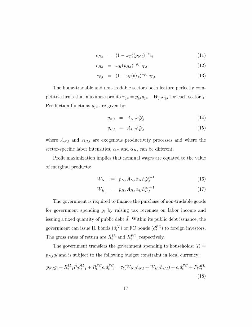
The home-tradable and non-tradable sectors both feature perfectly com-

petitive firms that maximize profits πj,t = pj,tyj,t −Wj,thj,t for each sector j.

Production functions yj,t are given by:

yN,t = AN,thαNN,t (14)

yH,t = AH,thαHH,t (15)

where AN,t and AH,t are exogenous productivity processes and where the

sector-specific labor intensities, αN and αH , can be different.

Profit maximization implies that nominal wages are equated to the value

of marginal products:

WN,t = pN,tAN,tαNhαN−1N,t (16)

WH,t = pH,tAH,tαHhαH−1H,t (17)

The government is required to finance the purchase of non-tradable goods

for government spending gt by raising tax revenues on labor income and

issuing a fixed quantity of public debt d. Within its public debt issuance, the

government can issue IL bonds (dILt ) or FC bonds (dFCt ) to foreign investors.

The gross rates of return are RILt and RFC

t , respectively.

The government transfers the government spending to households: Tt =

pN,tgt and is subject to the following budget constraint in local currency:

pN,tgt +RILt−1Ptd

ILt−1 +RFC

t−1etdFCt−1 = τt(WN,thN,t +WH,thH,t) + etd

FCt + Ptd

ILt

(18)

17

where expenses are on the left-hand side and revenues on the right-hand

side. FC bonds are pre-multiplied by the exchange rate because the budget

constraint is in local currency and IL bonds are pre-multiplied by the price

level because they are effectively real securities. Alfaro and Kanczuk (2010),

for example, introduce IL bonds in the budget constraints in the same way.

The timing is such that, bond levels chosen today have the t, and not t + 1

subscript.

The next subsection presents foreign investors utility maximization prob-

lem, which pins down bond rates, RILt and RFC

t , and provides empirical

support for all bonds being held abroad.

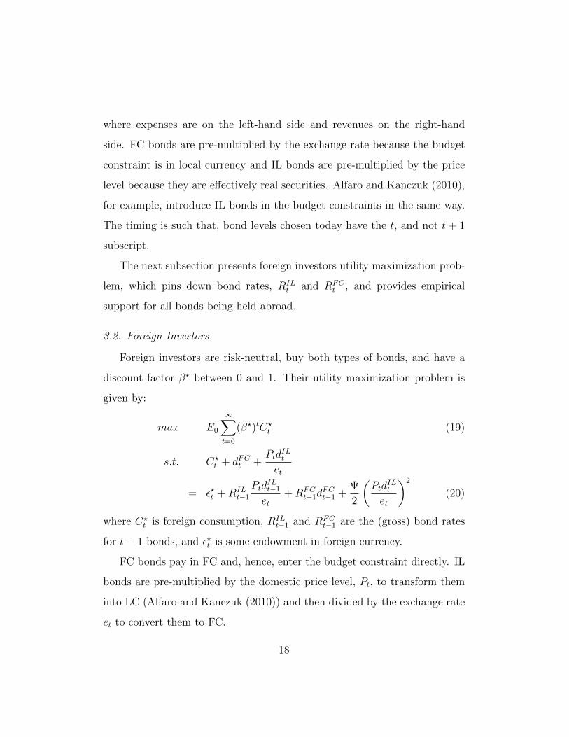
3.2. Foreign Investors

Foreign investors are risk-neutral, buy both types of bonds, and have a

discount factor β? between 0 and 1. Their utility maximization problem is

given by:

max E0

∞∑t=0

(β?)tC?t (19)

s.t. C?t + dFCt +

PtdILt

et

= ε?t +RILt−1

PtdILt−1

et+RFC

t−1dFCt−1 +

Ψ

2

(Ptd

ILt

et

)2

(20)

where C?t is foreign consumption, RIL

t−1 and RFCt−1 are the (gross) bond rates

for t− 1 bonds, and ε?t is some endowment in foreign currency.

FC bonds pay in FC and, hence, enter the budget constraint directly. IL

bonds are pre-multiplied by the domestic price level, Pt, to transform them

into LC (Alfaro and Kanczuk (2010)) and then divided by the exchange rate

et to convert them to FC.

18

Foreign investors are assumed to obtain a quadratic benefit of holding

IL debt. The model is agnostic about the source of this benefit, but it

allows the model to match,in steady state and for non-negative IL debt levels,

RILt < RFC

t , reported in section 2, fact 2. This modeling strategy is similar

to the one in Rabanal and Tuesta (2013), where a quadratic cost of holding

FC debt for domestic households introduces a wedge between LC and FC

rates 6.

Foreign investors’ optimization gives rise to the following gross rates of

return on FC and IL debt:

RFCt =

1

β?(21)

RILt =

1− ψ PtdILtet

β?Etπt+1

∆et+1

(22)

where πt+1 = Pt+1

Ptand ∆et+1 = et+1

et.

The intuition for the expressions are as follow. The FC bond, absent

default risk, is safe from the foreign investors’ perspective and, thus, to break-

even foreign investors only need to be promised the inverse of the discount

factor. The IL bond becomes more attractive, requiring a lower rate of return,

when investors expect inflation to increase, when investors expect a future

appreciation, and when the ad hoc benefit of holding IL debt increases.

The model features all public debt held abroad. This is line with the tra-

dition of studying external debt for emerging economies (Eaton and Gersovitz

(1981), Aguiar and Gopinath (2006), Arellano (2008)). More importantly, it

6Alternatively, the model in this study could feature a cost of holding FC debt for

foreign investors.

19

is consistent with the empirical evidence on FC and IL bond ownership. The

majority of external debt is in FC (Du and Schreger (2016), Ottonello and

Perez (Forthcoming)). There is also scattered evidence of foreign participa-

tion in IL debt markets. For example, 9% of 2016’s Brazilian external debt is

inflation-linked7 and 25% of the Russian 2015 IL debt issuance was bought by

foreign investors 8. Thus, it is consistent with the investor base composition

of FC and IL debt, that both bonds are priced by foreign investors.

3.3. Equilibrium

This subsection presents the model’s equilibrium conditions. Market

clearing in the public debt market and the non-tradable production sector,

respectively, imply that:

dILt + dFCt = d (23)

cN,t + gt = yN,t (24)

We define the value of exports, xt, and the value of imports, mt as:

xt = pH,t(yH,t − cH,t) (25)

mt = etcF,t (26)

7See the 2016 Annual Debt Report at (http://www.tesouro.

fazenda.gov.br/documents/10180/269444/RAD_2016_ingles_EN.pdf/

c3ae2138-7077-4c29-a383-3f3940f67311).8See the Russian Ministry of Finance Report titled ”A debut Issue of Sovereign

Inflation-Indexed Bonds by the Russian Federation” at http://old.minfin.ru/common/

upload/library/2015/09/main/OFZ-IN_case_study_ENG.pdf.

20

Finally, the economy’s position with respect to the rest of the world is

given by:

etdFCt + Ptd

ILt −RFC

t−1etdFCt−1 −RIL

t−1PtdILt−1 = mt − xt (27)

which states that trade deficits need to be financed by issuing external —

FC and IL — debt.

The equilibrium is given by a set of 22 unknowns {ct, cT,t, cN,t, cH,t, cF,t, hH,t,

hN,t,WH,t,WN,t, yN,t, yH,t, Pt, PT,t, pN,t, pH,t, et, dILt , d

FCt , RIL

t , RFCt , xt,mt} and

given exogenous processes {gt, τt, AN,t, AH,t}. The equilibrium must satisfy

households’ intratemporal optimality conditions (8) and (9); the demand

functions (10) to (13), the consumption and price indices definitions (3) to

(6); firms’ production functions and profit maximization conditions (14) to

(17); the government’s budget constraint (18); foreign investors’ breakeven

conditions (21) and (22); the definition for exports and imports (25) and

(26); and markets clearing conditions (23), (24), and (27).

3.4. Model calibration

Table 5 reports the parameter values used. For the inverse elasticity of

substitution, the model uses the standard value of σ = 2. Parameter ζ = 2

delivers a Frisch elasticity of 0.5, consistent with microeconometric estimates

(MaCurdy (1981), Altonji (1986), Chetty et al. (2011)). Most parameters in

the consumption indices and the production functions are similar to those

adopted by Schmitt-Grohe and Uribe (2018), who calibrate their model to 38

poor and emerging countries. One exception is the weight on home goods on

the tradable consumption index, which they calibrate to match a 20% average

export share in GDP in their sample. The average import and export share in

21

GDP in this study’s sample is somewhat higher — about 30% and the weight

on the home-tradable good reflects this. The foreign discount factor β? is

chosen to match the cross-sectional average FC rate in table (2) excluding

Argentina’s default. Finally, the parameter controlling the benefit of holding

IL debt, ψ, is small but able to deliver the smaller cross-sectional average IL

rate, as reported in table (2).

Parameter and symbol Value Reference

Inverse elasticity of substitution (σ) 2 Standard value

Inverse of Frisch elasticity (ζ) 2 Implies a Frisch elasticity 1ζ

= 0.5

Tradable weight in consumption index (ωT ) 0.5 Schmitt-Grohe and Uribe (2018)

Elasticity of substitution between cT and cN (ρ) 1 Schmitt-Grohe and Uribe (2018)

Weight on home good in tradable consumption (ωH) 0.3 Matches average sample import share of GDP of 30%

Elasticity of substitution between cH and cF (ρT ) 0.5 Schmitt-Grohe and Uribe (2018)

Labor share in non-tradable production (αN) 0.75 Schmitt-Grohe and Uribe (2018)

Labor share in tradable production (αH) 0.65 Schmitt-Grohe and Uribe (2018)

Foreign discount factor (β?) 0.94 Matches net rate of return rFC = 6.4%

Benefit of holding IL debt (ψ) 0.17 Small, but able to deliver rIL < rFC

Table 5: Parameter values

Table 6 compares key variables delivered by the model in steady state with

the average emerging economy in the data. The model effectively replicates

the debt over GDP, the share of debt linked to inflation, government spending

over GDP, and tax revenues over GDP. The model also replicates the cross-

sectional average of the IL rate, which equals 4.6% in the sample (table (2))

and 4.7% in the model’s steady-state.

The next section uses this model to deliver stylized facts 3 to 5 in section

2.

22

Variable Data Model

Debt over GDP 45.1% 46.1%

IL debt over Debt 13.3% 15.9%

Government spending over GDP 15.5% 14.6%

Tax revenues over GDP 15.5% 17.6%

IL rate 4.6% 4.7%

Table 6: Comparison between the model ratios and IL bond rate and the data for the

average emerging economy in the study’s sample.

4. Results

4.1. Key result on FC and IL debt substitution

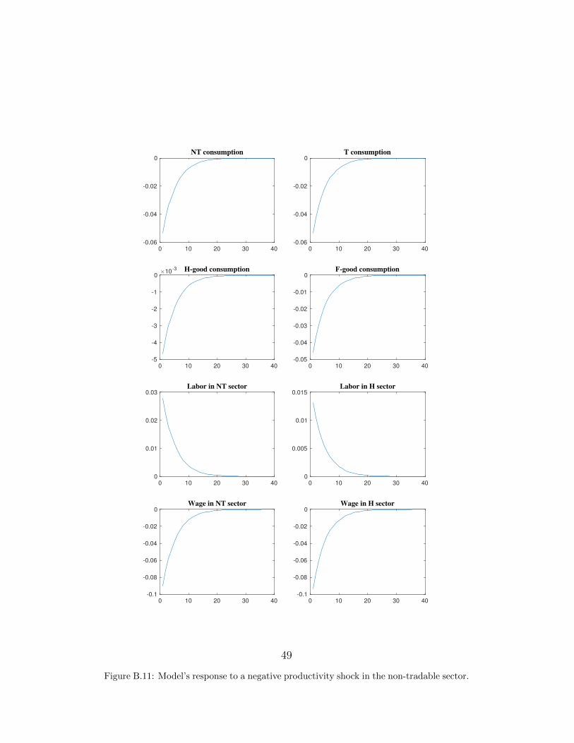
This subsection presents the model’s response to a negative productivity

shock in the non-tradable sector, aN,t.

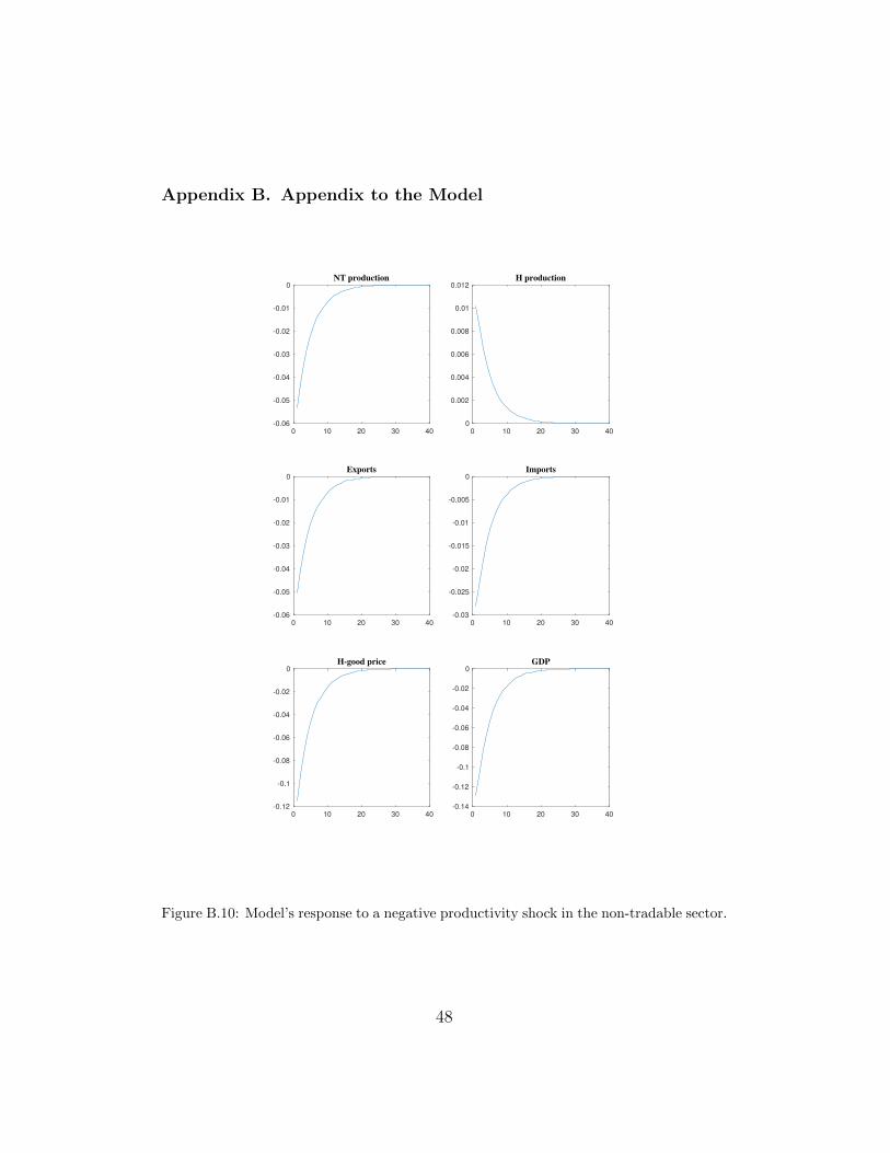
Figure 1 as well as figures B.11 and B.10 in Appendix B show the impulse

response functions of the model to a negative productivity shock in the non-

tradable sector with respect to the steady state, turning off all other shocks.

They show that, after a negative productivity shock in the non-tradable

sector of 10%, the wage rate in this sector decreases by the same amount.

The income effect of the lower wage dominates the substitution effect and

labor supply in the non-tradable sector increases by 3%. The labor supply

increase partly dampens the effect of the productivity shock on non-tradable

output, which only falls by 5%.

For a given level of government spending, a drop in the non-tradable

production, by market clearing condition (24), implies a drop in the non-

tradable consumption. This causes the demand for the remaining goods to

23

0 10 20 30 40

-0.15

-0.1

-0.05

0

Consumption

0 10 20 30 40

-0.025

-0.02

-0.015

-0.01

-0.005

0

Tax revenues

0 10 20 30 40

0

0.02

0.04

0.06

Exchange rate

0 10 20 30 40

-0.02

0

0.02

0.04

0.06

Exchange rate growth

0 10 20 30 40

0

0.1

0.2

0.3

0.4

IL debt

0 10 20 30 40

-0.4

-0.3

-0.2

-0.1

0

FC debt

0 10 20 30 40

-0.6

-0.4

-0.2

0

IL debt rate

0 10 20 30 40

-0.1

-0.08

-0.06

-0.04

-0.02

Productity in NT sector

Figure 1: Model’s response to a negative productivity shock in the non-tradable sector.

24

also fall, due to the complementarity between goods that demand equations

(10)-(13) exhibit.

The drop in the demand for foreign goods, cF,t, depreciates the exchange

rate, as equation (13) shows. The depreciation of 6% implies that the domes-

tic economy is only capable of financing smaller trade deficits (see equation

(27)) — exports drop by 5% whereas imports only drop by 3%.

The drop in demand for home-tradable goods at home and abroad de-

creases their price, pH,t, decreasing the value of the marginal product of labor

in the home-tradable sector and, thus, decreasing the sector’s wage. As be-

fore, the income effect of the lower wage dominates the substitution effect

and labor supply in the home-tradable sector increases.

Tax revenues fall by 2% because the increases in the labor supply in both

sectors are insufficient to compensate the larger sectoral wage falls.

The current exchange rate depreciation, jointly with the law of motion

for the productivity shock, causes an expected future appreciation of the

currency, ∆et+1 = et+1

et, which decreases the IL rate, as it is clear from equa-

tion (22). The fourth panel in figure 1 shows the future appreciation. The

magnitude of the rate decrease is 50%, which, for the average economy, the

model is calibrated to, implies a decrease in the IL rate from 4.7% to 2.4%.

FC debt, on the contrary, still requires a 6.4% interest rate.

Finally, IL debt issuance increases by 35% and FC debt issuance decreases

by 35%. For the average emerging economy, the model is calibrated to, this

implies six percentage points increase in the IL debt issuance. This happens,

in the model, because for the government’s budget constraint (18) to balance

in period t + 1, a lower interest rate implies IL debt needs to increase. If

25

public debt composition were chosen actively by the government, it would

also choose to move towards IL debt because it becomes cheaper to borrow

in this manner.

The total IL rate decrease is, partially, a result of the IL rate’s dependance

on the level of IL debt through the 1 − ψ Ptdtet

term. The next subsection

presents the IL rate decrease if ψ = 0.

4.2. IL rate dynamics if ψ = 0

When ψ = 0, foreign investors do not enjoy any benefit from holding IL

debt versus FC debt. Because in steady state, πt+1 = et+1 = 1, equations

(21) and (22) imply that the (gross) interest rate for both bonds is the same

and equal to 1β?

. Hence, ψ = 0 precludes the model from delivering a steady-

state interest rate differential between both bonds. It is still interesting to

study the dynamics in this case for two reasons. First, it helps us understand

the workings of the model and, second, it determines the magnitude of the

interest rate fluctuations when the mechanical feedback between IL debt and

IL rate is absent.

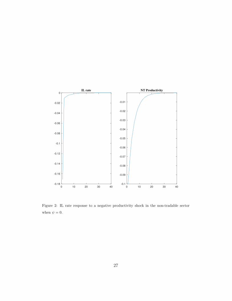
Figure (2) shows the response of the IL rate to a 10% negative produc-

tivity shock in the non-tradable sector, aN,t in the model with ψ = 0. The

qualitative responses of the model are identical to the ones in the previous

subsection but the IL rate drop is smaller. Indeed, the IL rate falls by 17%,

which, for the average economy, the model is calibrated to, implies a drop

from 6.4% to 5.3%. This is evidence that a large portion of the IL rate drop

in the previous subsection is coming from the mechanical effect IL debt has

on IL rates.

The model’s key takeaway is that, during crises, borrowing in IL debt

26

0 10 20 30 40

-0.18

-0.16

-0.14

-0.12

-0.1

-0.08

-0.06

-0.04

-0.02

0

IL rate

0 10 20 30 40

-0.1

-0.09

-0.08

-0.07

-0.06

-0.05

-0.04

-0.03

-0.02

-0.01

NT Productivity

Figure 2: IL rate response to a negative productivity shock in the non-tradable sector

when ψ = 0.

27

becomes cheaper because, for a short-lived recession, foreign investors expect

a future appreciation. The next subsection evaluates the empirical support

for the model’s findings on IL rates during crises.

5. IL, FC, and LC rates

This section investigates whether, like the model predicts, IL rates fall

during crises. Furthermore, it returns to the findings on IL, FC, and LC rates

of fact 2 in section 2 and explores whether the rate differentials uncovered

can be explained by expected infaltion rates and expected exchange rate

variations.

5.1. IL rates during crises

In the study’s sample, there are 11 crisis episodes, for which the IL rate is

available. A crisis episode for a country is a year when its real GDP growth

rate is negative. Out of these 11 episodes, 6 of them are accompanied by

decreases in the IL rate and 5 are not. Table 7 lists each of the episodes

and categorizes them as simultaneously exhibiting an IL rate decrease or

not. Between parantheses are the magnitudes of the IL rate decrease in

percentage terms.

A crisis episode in which the IL rate fails to drop is consistent with this

study’s model if the crisis is persistent. Indeed, if next period’s exchange

rate, et+1, is expected to fall further than in period t, then investors expect

a future depreciation, ∆et+1 drops, and the IL rate increases. Studying the

relationship between the behavior of IL rates and the crisis persistance is left

for future work.

28

Crisis episodes and behavior of IL rates

IL rate drop IL rate increase

Argentina, 2014 (-44.1%) and 2016 (-73.5%) Argentina, 2009 and 2012

Brazil, 2009 (-9.7%) and 2016 (-6.3%) Brazil 2015

Chile 2009 (-8.6%) Mexico 2009

Russia 2016 (-12.2%) South Africa 2009

Table 7: Crisis episodes and behavior of IL rates

To sum-up, more than half of the crisis episodes simultaneously exhibit

a decrease in the IL rate. However, the evidence is mixed. For 5 crises, IL

rates failed to drop and it is unclear, at this point, that these were the most

persistent crises. Exploring further the behavior of IL rates during crises is

a possible topic for future research.

5.2. Role of expected inflation and expected exchange rate variations

Fact 2 in section 2 shows that, in the cross-section, RFCt > RIL

t . Column

2 in table 8 reports the average FC-IL rate differential by country and, in the

last row, shows that the differential is 0.9% on average, when excluding Ar-

gentina’s default episode. Model equations (21) and (22) show that expected

inflation and expected exchange rate variations can explain a positive FC-IL

rate differential.

Fact 2 in section 2 also shows that, in the cross-section, RLCt > RIL

t .

Column 3 in table 8 reports the average LC-IL rate differential by country

and, in the last row, shows that the differential is, on average, 4%. To

complete the analysis, we need the theoretical expression for the LC rate.

29

To do this, from equation (20), the new budget constraint for foreign

investors that can buy LC debt, dLCt , is given by:

C?t +dFCt +

PtdILt

et+dLCtet

= ε?t+RILt−1

PtdILt−1

et+RFC

t−1dFCt−1+

Ψ

2

(Ptd

ILt

et

)2

+RLCt−1

dLCt−1

et(28)

where dLCt is divided by the exchange rate, et, to transform the payment to

FC.

Maximizing (19) subject to (28), instead of subject to (20), gives the

following expression for the LC rate:

RLCt =

1

β?Et1

∆et+1

(29)

Equations (29) and (22) show that expected inflation can explain the

positive LC-IL rate differential. Indeed, from equations (21), (22), and (29),

the following rate differentials emerge:

rFCt − rILt ≈ Et(πt+1)− Et(∆et+1) (30)

rLCt − rILt ≈ Et(πt+1) (31)

where r denote net rates of return for the different bonds — LC, IL, and

FC — and the variables with tildes denote the net rate of inflation and net

depreciation rate9.

To account for these expectations, I use the averages of the 4-year ahead

consensus forecasts of the inflation rate and the nominal exchange rate from

FocusEconomics. See Appendix A for coverage and definitions.

9Note that foreign inflation cancels out in the calculation of the rate differentials.

Intuitively, foreign inflation increases the interest foreign investors require on all bonds.

30

Longer-term forecasts, instead of one-year ahead forecasts, are necessary

because the rates come from medium and long-term bonds. Unfortunately,

long-term forecasts, especially for the nominal exchange rate, are not publicly

available and, even within proprietary datasets, are hard to find for long

horizons and with substantial historical coverage.

In the FocusEconomics data, the 4-year expected inflation rate is given in

annual terms and the 4-year expected nominal exchange rate is given in units

of LC needed to purchase 1 USD. Using the current level of the exchange, I

can calculate the expected rate of depreciation over a 4-year interval. How-

ever, there is a time period mismatch between expected inflation rate and

expected rate of depreciation. For this reason, I calculate annualized depreci-

ation rates by dividing the total expected depreciation by 4, assuming, thus,

that the total expected rate of depreciation is spread out smoothly over the

4-year period10.

Using the 4-year ahead expected inflation rate and the imputed 4-year

ahead depreciation rate, I recalculate the interest rate differentials in columns

2 and 3 adjusting the IL rates as follows:

r1,adj = rILt + Et(πt+1)− Et(∆et+1) (32)

r2,adj = rILt + Et(πt+1) (33)

where the first expression is used to compare IL rates to FC rates and the

second expression is used to compare IL rates to LC rates. The results are

10An alternative is to use the expected variation in the price index (e.g. CPI) over a

4-year window. However, to the best of my knowledge, expected price indices are not

collected by Central Banks’ surveys nor private companies.

31

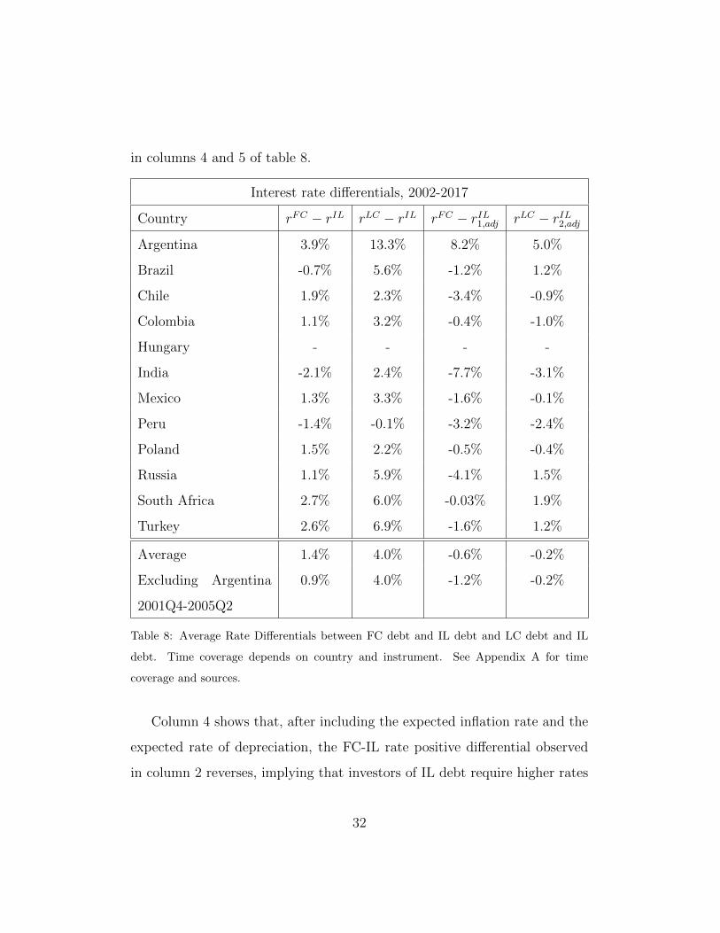
in columns 4 and 5 of table 8.

Interest rate differentials, 2002-2017

Country rFC − rIL rLC − rIL rFC − rIL1,adj rLC − rIL2,adj

Argentina 3.9% 13.3% 8.2% 5.0%

Brazil -0.7% 5.6% -1.2% 1.2%

Chile 1.9% 2.3% -3.4% -0.9%

Colombia 1.1% 3.2% -0.4% -1.0%

Hungary - - - -

India -2.1% 2.4% -7.7% -3.1%

Mexico 1.3% 3.3% -1.6% -0.1%

Peru -1.4% -0.1% -3.2% -2.4%

Poland 1.5% 2.2% -0.5% -0.4%

Russia 1.1% 5.9% -4.1% 1.5%

South Africa 2.7% 6.0% -0.03% 1.9%

Turkey 2.6% 6.9% -1.6% 1.2%

Average 1.4% 4.0% -0.6% -0.2%

Excluding Argentina

2001Q4-2005Q2

0.9% 4.0% -1.2% -0.2%

Table 8: Average Rate Differentials between FC debt and IL debt and LC debt and IL

debt. Time coverage depends on country and instrument. See Appendix A for time

coverage and sources.

Column 4 shows that, after including the expected inflation rate and the

expected rate of depreciation, the FC-IL rate positive differential observed

in column 2 reverses, implying that investors of IL debt require higher rates

32

of return than merely the expected inflation and expected depreciation rate

suggest.

Column 5 shows some cross-country heterogeneity. The positive LC-IL

rate differential remains, even after including the expected inflation rate, for

5 of the 11 countries considered, implying that, for these countries, investors

of LC debt require higher rates of return than the expected inflation would

suggest. This is consistent with an inflation risk-premium, that is, investors

requiring an additional premium to bear inflation risk (Bekaert and Wang

(2010), Ermolov (2018)). For these countries, IL debt seems an attractive

form of debt financing.

Understanding the drivers behind the rate differentials is outside the scope

of this paper. Instead, the previous analysis takes the rate levels as given and

explores the behavior of IL rates over the business cycle and how it affects

emerging economies’ public debt composition, in particular the substitution

of FC debt for IL debt.

6. Conclusions

The study reports a set of stylized facts about recent emerging economies’

IL public debt issuance. On average, emerging economies issue 13% of their

public debt linked to inflation. This represents 23% of their LC public debt.

The evidence on IL, FC, and LC rates, shows that, for half of the countries

in the study’s sample, IL rates are below LC rate, even after accounting for

expected inflation rates. The paper also uncovers the following business-cycle

properties of IL debt issuance — it is countercyclical, increases amid nominal

exchange rate depreciations, and substitutes FC and non-indexed LC debt.

33

Subsequently, the study presents a two-sector small-open economy model

of public debt composition that can deliver the business cycle properties of

IL debt issuance. Moreover, the model shows that, during economic crises,

when the economy endures a nominal exchange rate depreciation, IL debt

becomes cheaper to issue. Finally, the study shows evidence of IL rates

falling in about half of the recent crises in emerging economies.

This study has relevant policy implications. IL debt is an attractive

instrument for some of the governments in the study’s sample, since, for

them, IL rates are, on average, below LC rates, even after accounting for

expected inflation rates. Indeed, for these countries, IL rates are between

1.2 and 5 percentage points lower than LC rates. Moreover, the study’s

model shows that, IL debt can be a especially beneficial debt instrument

to use during economic crises, as IL rates drop amid nominal exchange rate

depreciations.

Exploring the cross-sectional variation in the amount of IL debt emerg-

ing economies issue, as well as why some economies (e.g. Czech Republic,

Indonesia, Malaysia, and Thailand) avoid issuing this debt, is a promising

avenue for future research. Studying further the behavior of IL rates during

crises can help clarify when is IL debt a good debt instrument to finance

government spending. Finally, exploring the negative FC-IL rate differential

when accounting for expected inflation and expected exchange rate varia-

tions, as well as the cross-sectional variation in the LC-IL rate differential

when accounting for expected inflation can shed light on the institutional

determinants of IL debt being an attractive form of debt financing.

34

Appendix A. Appendix to the Empirical Evidence

Appendix A.1. Sample, sources, and coverage of key variables

Sample of countries and corresponding regions

Region? Countries in sample

Latin America Argentina, Brazil, Chile, Colombia, Mexico, Peru

EMEA-UE Hungary, Poland

EMEA-non UE India, Russia, South Africa, Turkey

Table A.9: Sources and coverage for IL rates for all countries in sample. ? Asian economies

such as Indonesia, Malaysia or Thailand are not included in the study because they do

not issue this type of public debt. The same happens with Czech Republic. See Table C2

in https://www.bis.org/statistics/secstats.htm.

1. IL debt issuance: Bank of International Settlements. Table C2.

Link: https://www.bis.org/statistics/secstats.htm. Available

at yearly frequency only, 1995-2016.

2. Total government debt and local currency government debt:

Arslanalp and Tsuda (2014), 2004-2016.

3. REER: Darvas (2012), 1995-2016.

4. All other macroaggregates: World Development Indicators (WDI),

1995-2016.

5. FC bond rate: JP Morgan EMBI+, yield-to-maturity, 1995Q1-2017Q4.

6. LC bond rate: JP Morgan GBI-EM, yield-to-maturity. End date:

2017Q4. Starting dates: Argentina (2007Q3), Brazil (2002Q1), Chile

(2002Q4), Colombia (2005Q1), Hungary (2001Q1), India (2000Q1),

35

Mexico (2002Q1), Peru (2006Q4), Poland (2001Q1), Russia (2005Q1),

South Africa (2000Q1), Turkey (2000Q1).

7. IL bond rate:

IL bond rate: coverage and sources

Country Source Bloomberg Ticker or Link Coverage

Argentina Barclays BEMA8y Index 2003Q4-2017Q3

Brazil Bloomberg TRBRI15 2006Q1-2017Q3

Chile Barclays BEMC8y Index 2002Q3-2017Q3

Colombia Barclays BEMy8y Index 2003Q4-2017Q3

Hungary - - -

India S&P Index https://us.spindices.com/indices/fixed-income/

sp-india-sovereign-inflation-linked-bond-index

2013Q3-2017Q3

Mexico Barclays BEMM8y Index 2006Q1-2017Q3

Peru S&P Index https://us.spindices.com/indices/fixed-income/

sp-peru-sovereign-inflation-linked-bond-index

2008Q2-2017Q3

Poland Barclays BEMv0y Index 2003Q3-2017Q3

Russia Barclays Brulcy Index 2015Q3-2017Q3

South Africa Bloomberg MLGSail 2004Q1-2017Q3

Turkey Bloomberg TRTKI5y 2013Q2-2017Q3

Table A.10: Sources and coverage for IL rates for all countries in sample.

Appendix A.2. Coverage and definitions of expectations data

1. Expected exchange rate: 4-year ahead expected nominal exchange

rate, units of LC per USD. Eg. 2013 forecast of the nominal exchange

rate in 2017. Source: FocusEconomics.

2. Expected inflation rate: 4-year ahead expected annual variation in

the CPI. Source: FocusEconomics.

36

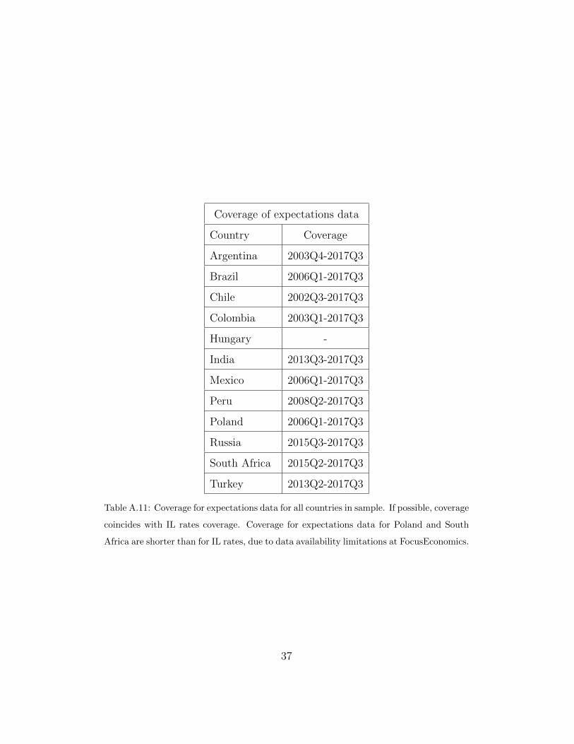
Coverage of expectations data

Country Coverage

Argentina 2003Q4-2017Q3

Brazil 2006Q1-2017Q3

Chile 2002Q3-2017Q3

Colombia 2003Q1-2017Q3

Hungary -

India 2013Q3-2017Q3

Mexico 2006Q1-2017Q3

Peru 2008Q2-2017Q3

Poland 2006Q1-2017Q3

Russia 2015Q3-2017Q3

South Africa 2015Q2-2017Q3

Turkey 2013Q2-2017Q3

Table A.11: Coverage for expectations data for all countries in sample. If possible, coverage

coincides with IL rates coverage. Coverage for expectations data for Poland and South

Africa are shorter than for IL rates, due to data availability limitations at FocusEconomics.

37

Appendix A.3. Tables and graphs0

20

40

60

80

IL D

eb

t, a

s %

of

tota

l

2005 2010 2015Years

Argentina Brazil

Chile Colombia

Mexico South Africa

Turkey

IL Debt over Public Debt in Emerging Economies (I)

Figure A.3: Share of IL debt (as % of Total Public Debt) for Emerging Economies (I), by

country. Data sources: see above.

38

Results of Stationarity Tests

Variable Number of lags (AIC) Wt p-value

ILD 0.58 1.654 0.951

GDP 0.25 8.909 1.000

FC Debt 0.33 2.504 0.994

Nominal Debt 0.08 4.910 1.000

Debt 0.33 6.127 1.000

Exchange rate 0.75 2.702 0.997

REER 0.50 -0.828 0.205

GDP Deflator 0.33 11.460 1.000

CPI 0.73 8.560 1.000

Table A.12: Wt is the statistic in Im et al. (2003) unit root tests for panel data with het-

erogenous panels. Im et al. (2003) does not require balanced panels. The null hypothesis,

H0, is that all panels contain unit roots. The alternative hypothesis, Ha, is that at least

one panel is stationary. Number of lags are chosen using the Akaike information criterion

(AIC). Using the bayesian information criterion (BIC) or Hannan-Quinn information cri-

terion (HQIC), including a trend and/or subtracting the cross-sectional averages from the

series to mitigate the impact of cross-sectional dependance leaves the conclusions of the

tests above unchanged.

39

Dates of IL debt issuance start and IT adoption

Country IL debt issuance start IT adoption date

Argentina 2002 2017

Brazil 1964 1999

Chile 1956 1999

Colombia 1967 1999

Hungary 2011 2001

India 1998 2015

Mexico 1989 2001

Peru 2003 2002

Poland 2004 1998

Russia 2004? 2015

South Africa 2000 2000

Turkey 2000? 2006

Table A.13: Dates of IL debt issuance start and IT adoption. Sources for IL debt is-

suance start: BIS Table C2. For Mexico IL debt start: Barclays (2004), p. 58. For

Brazil, Chile and Colombia: Godoy et al. (2009). ?For Russia and Turkey, study’s

data starts in, respectively, 2004 and 2000 but previous years are missing (not zero).

Sources for IT adoption date: Jahan (2012). For Argentina: slide 5 ”Regimen de

metas de inflacion en Argentina” presentation from Banco Central de la Republica

Argentina, September 2016 (https://www.bcra.gob.ar/Pdfs/Prensa_comunicacion/

Metas_de_inflacion26092016.PDF). For India Reserve Bank of India press release men-

tioned in Bloomberg article ”India keeps Rajan’s inflation target as his term nears end”,

August 5, 2016. For Russia Korhonen and Nuutilainen (2017).

40

Increases in IL debt over time, 2004-2016

Country ∆ (IL debt/debt)

Argentina -12.6%

Brazil 12.6%

Chile 37.5%

Colombia 2%

Hungary 4%

India -0.04%

Mexico 10.6%

Peru 2.1%

Poland -0.3%

Russia 0.9%

South Africa 12.0%

Turkey 1.8%

Table A.14: Increases in IL debt over Total Public Debt between 2004 and 2016. Source:

See above.

41

01

23

4IL

De

bt,

as %

of

tota

l

2000 2005 2010 2015Years

Hungary India

Peru Poland

Russia

IL Debt over Public Debt in Emerging Economies (II)

Figure A.4: Share of IL debt (as % of Total Public Debt) for Emerging Economies (II),

by country. Data sources: see above.

42

20

40

60

80

100

FC

Debt, a

s %

of to

tal

020

40

60

80

IL D

ebt, a

s %

of to

tal

2005 2010 2015time

IL Debt FC Debt

Chile

30

40

50

60

FC

Debt, a

s %

of to

tal

01

23

4IL

Debt, a

s %

of to

tal

2005 2010 2015time

IL Debt FC Debt

Hungary

010

20

30

40

FC

Debt, a

s %

of to

tal

510

15

20

IL D

ebt, a

s %

of to

tal

2005 2010 2015time

IL Debt FC Debt

Mexico

40

60

80

100

FC

Debt, a

s %

of to

tal

11.5

22.5

33.5

IL D

ebt, a

s %

of to

tal

2005 2010 2015time

IL Debt FC Debt

Peru

IL Debt vs FC Debt (as % of total debt), 2004−2016

Figure A.5: Share of IL debt and FC debt (as % of Total Government Debt) for a selection

of emerging economies. Data sources: see above.

43

01

02

03

04

05

0P

erc

en

tag

e,

%

1995q1 2000q1 2005q1 2010q1 2015q1 2020q1Quarters

FC Rate IL Rate

Argentina

Figure A.6: Foreign currency (FC) and inflation-linked (IL) bond rates between 2002 and

2017 for Argentina. Data sources: see above.

44

0102030 0102030 0102030

20

00

q1

20

06

q1

20

12

q1

20

18

q1

20

00

q1

20

06

q1

20

12

q1

20

18

q120

00

q1

20

06

q1

20

12

q1

20

18

q120

00

q1

20

06

q1

20

12

q1

20

18

q1

Bra

zil

Ch

ileC

olo

mb

iaH

un

ga

ry

Ind

iaM

exic

oP

eru

Po

lan

d

Ru

ssia

So

uth

Afr

ica

Tu

rke

y

FC

Ra

te I

L R

ate

Percentage, %

Qu

art

ers

Gra

ph

s b

y c

ou

ntr

y

Fig

ure

A.7

:F

orei

gncu

rren

cy(F

C)

and

infl

ati

on

-lin

ked

(IL

)b

on

dra

tes

bet

wee

n2002

an

d2017.

Sou

rces

:se

eab

ove.

45

02

04

06

08

0

1995q1 2000q1 2005q1 2010q1 2015q1 2020q11995q1 2000q1 2005q1 2010q1 2015q1 2020q1

Argentina Turkey

LC Rate IL Rate

Pe

rce

nta

ge

, %

Quarters

Graphs by country

Figure A.8: Local currency (LC) and inflation-linked (IL) bond rates between 2002 and

2017 for Argentina and Turkey. Data sources: see above.

46

0102030 0102030 0102030

19

95

q120

00

q120

05

q120

10

q120

15

q120

20

q119

95

q120

00

q120

05

q120

10

q120

15

q120

20

q1

19

95

q120

00

q120

05

q120

10

q120

15

q120

20

q119

95

q120

00

q120

05

q120

10

q120

15

q120

20

q1

Bra

zil

Ch

ileC

olo

mb

iaH

un

ga

ry

Ind

iaM

exic

oP

eru

Po

lan

d

Ru

ssia

So

uth

Afr

ica

LC

Ra

teIL

Ra

te

Percentage, %

Qu

art

ers

Gra

ph

s b

y c

ou

ntr

y

Fig

ure

A.9

:L

oca

lcu

rren

cy(L

C)

an

din

flati

on

-lin

ked

(IL

)b

on

dra

tes

bet

wee

n2002

an

d2017.

Sou

rces

:se

eab

ove.

47

Appendix B. Appendix to the Model

0 10 20 30 40

-0.06

-0.05

-0.04

-0.03

-0.02

-0.01

0

NT production

0 10 20 30 40

0

0.002

0.004

0.006

0.008

0.01

0.012

H production

0 10 20 30 40

-0.06

-0.05

-0.04

-0.03

-0.02

-0.01

0

Exports

0 10 20 30 40

-0.03

-0.025

-0.02

-0.015

-0.01

-0.005

0

Imports

0 10 20 30 40

-0.12

-0.1

-0.08

-0.06

-0.04

-0.02

0

H-good price

0 10 20 30 40

-0.14

-0.12

-0.1

-0.08

-0.06

-0.04

-0.02

0

GDP

Figure B.10: Model’s response to a negative productivity shock in the non-tradable sector.

48

0 10 20 30 40

-0.06

-0.04

-0.02

0

NT consumption

0 10 20 30 40

-0.06

-0.04

-0.02

0

T consumption

0 10 20 30 40

-5

-4

-3

-2

-1

010

-3 H-good consumption

0 10 20 30 40

-0.05

-0.04

-0.03

-0.02

-0.01

0

F-good consumption

0 10 20 30 40

0

0.01

0.02

0.03

Labor in NT sector

0 10 20 30 40

0

0.005

0.01

0.015

Labor in H sector

0 10 20 30 40

-0.1

-0.08

-0.06

-0.04

-0.02

0

Wage in NT sector

0 10 20 30 40

-0.1

-0.08

-0.06

-0.04

-0.02

0

Wage in H sector

Figure B.11: Model’s response to a negative productivity shock in the non-tradable sector.

49

References

Aguiar, M., Amador, M., Hopenhayn, H., Werning, I., November 2016. Take

the short route: equilibrium default and debt maturity. Mimeo.

Aguiar, M., Gopinath, G., 2006. Defaultable debt, interest rates and the

current account. Journal of International Economics 69 (1), 64–83.

Alfaro, L., Kanczuk, F., 2010. Nominal versus indexed debt: a quantitative

horserace. Journal of International Money and Finance 29, 1706–1726.

Altonji, J., 1986. Intertemporal substitution in labor supply: evidence from

micro data. Journal of Political Economy 94 (3), S176–S215.

Arellano, C., 2008. Default risk and income fluctuations in emerging

economies. American Economic Review 98 (3), 690–712.

Arellano, C., Ramanarayanan, A., April 2012. Default and the maturity

structure in sovereign bonds. Journal of Political Economy 120 (2), 187–

232.

Arslanalp, S., Tsuda, T., 2014. Tracking global demand for emerging market

sovereign debt. IMF Working Paper (14/39).

Barclays, 2004. Global inflation-linked products: A user’s guide. Barclays

Capital Research.

Bekaert, G., Wang, X., October 2010. Inflation risk and the inflation risk

premium. Economic Policy 25 (64), 755–806.

50

Bocola, L., Dovis, A., September 2016. Self-fulfilling debt crises: A quanti-

tative analysis. Mimeo.

Bohn, H., 1988. Why do we have nominal government debt? Journal of

Monetary Economics 21 (1), 127–140.

Bohn, H., 1990. Tax smoothing with financial instruments. American Eco-

nomic Review 80 (5), 1217–1230.

Broner, F., Lorenzoni, G., Schmukler, S., 2013. Why do emerging economies

borrow short-term? Journal of the European Economic Association

11 (S1), 67–100.

Calvo, G., Guidotti, P. E., 1990. Indexation and maturity of government

bonds: an exploratory model. In: Public debt managament: theory and

history. Cambridge University Press.

Chetty, R., Mannoli, D., Weber, A., May 2011. Are micro and macro labor

supply elasticities consistent? a review of evidence on the intensive and

extensive margins. American Economic Review Papers and Proceedings.

Corsetti, G., Dedola, L., Leduc, S., April 2008. International risk sharing

and the transmission of productivity shocks. Review of Economic Studies

75 (2), 443–473.

Darvas, Z., 2012. Real effective exchange rates for 178 countries: a new

database. Bruegel Working Paper (2012/06).

Diaz-Gimenez, J., Giovanetti, G., Marimon, R., Teles, P., 2008. Nominal

51

debt as a burden to monetary policy. Review of Economic Dynamics 11,

493–514.

Du, W., Schreger, J., June 2016. Local currency sovereign risk. Journal of

Finance 71 (3), 1027–1070.

Du, W., Schreger, J., Pflueger, C. E., September 2016. Sovereign bond port-

folios, bond risks and credibility of monetary policy. Mimeo.

Eaton, J., Gersovitz, M., 1981. Debt with potential repudiation: theoretical

and empirical analysis. Review of Economic Studies 48, 289–309.

Eichengreen, B., Hausmann, R., Panizza, U., 2005. The mystery of the orig-

inal sin. Vol. Other people’s money: Debt denomination and financial in-

stability in emerging-market economies. The mystery of the original sin.

Eichengreen, B., Hausmann, R., Panizza, U., 2007. Currency Mismatches,

Debt Intolerance, and the Original Sin: Why They Are Not the Same and

Why It Matters. Vol. Capital Controls and Capital Flows in Emerging

Economies: Policies, Practices and Consequences. University of Chicago

Press.

Engel, C., Park, J., November 2017. Debauchery and original sin: The cur-

rency composition of sovereign debt. Mimeo.

Ermolov, A., November 2018. When and where is it cheaper to issue inflation-

linked debt? SSRN Working Paper (2998687).

Fernandez, R., Martin, A., September 2015. The long and the short of it:

Sovereign debt crises and debt maturity. Mimeo.

52

Fleckenstein, M., Longstaff, F. A., Lustig, H., 2014. The TIPS-Treasury bond

puzzle. The Journal of Finance LXIX (5), 2151–2197.

Godoy, G., Casanueva, C., Ruiz, F., Solana, P., 2009. Indexacion financiera:

ventajas y desventajas de contar con una unidad de cuenta indexada a la

inflacion en espana. XIII Congreso de ingenierıa de organizacion.

Im, K. S., Pesaran, M., Shin, Y., January 2003. Testing for unit roots in

heterogeneous panels. Journal of Econometrics 115, 53–74.

Jahan, S., March 2012. Inflation targeting: holding the line. IMF Finance

and Development.

Jeanneret, A., Souissi, S., 2016. Sovereign defaults by currency denomination.

Journal of International Money and Finance 60, 197–222.

Korhonen, I., Nuutilainen, R., 2017. Breaking monetary policy rules in Rus-

sia. Russian Journal of Economics 3, 366–378.

MaCurdy, T. E., 1981. An empirical model of labor supply in a life-cycle

setting. Journal of Political Economy 89 (6), 1059–1085.

Mendoza, E., 1995. The terms of trade, the real exchange rate, and economic

fluctuations. International Economic Review 36 (1), 101–137.

Ottonello, P., Perez, D., Forthcoming. The currency composition of sovereign

debt. American Economic Journal: Macroeconomics.

Rabanal, P., Tuesta, V., 2013. Nontradable goods and the real exchange rate.

Open Economies Review 24 (3), 495–535.

53

Schmitt-Grohe, S., Uribe, M., February 2018. How important are terms-of-

trade shocks? International Economic Review 59 (1), 85–111.

Stockman, A., Tesar, L., 1995. Tastes and technology in a two-country model

of the business cycle: Explaining international comovements. American

Economic Review 85 (1), 168–185.

Sunder-Plassmann, L., February 2017. Inflation, default, and sovereign debt:

The role of denomination and ownership. Mimeo.

54