NBER WORKING PAPER SERIES

IMPULSIVE CONSUMPTION AND FINANCIAL WELLBEING:EVIDENCE FROM AN INCREASE IN THE AVAILABILITY OF ALCOHOL

Itzhak Ben-DavidMarieke Bos

Working Paper 23211http://www.nber.org/papers/w23211

NATIONAL BUREAU OF ECONOMIC RESEARCH1050 Massachusetts Avenue

Cambridge, MA 02138March 2017

We thank Anna Dreber-Almenberg, Roc Armenter, Laurent Bach, Bruce Carlin, Hans Grönqvist, DavidLaibson, Christine Laudenbach, Susan Niknami, Leonard Nakamura, Martin Schmaltz, and numerousseminar and conference participants for helpful comments. Jesper Böjeryd and Johan Orrenius providedexcellent research assistance. Funding from VINNOVA is gratefully acknowledged. All errors areour own. The views expressed here are those of the authors and do not necessarily represent thoseof the Federal Reserve Bank of Philadelphia, the Federal Reserve System, or the National Bureau ofEconomic Research.

NBER working papers are circulated for discussion and comment purposes. They have not been peer-reviewed or been subject to the review by the NBER Board of Directors that accompanies officialNBER publications.

© 2017 by Itzhak Ben-David and Marieke Bos. All rights reserved. Short sections of text, not to exceedtwo paragraphs, may be quoted without explicit permission provided that full credit, including © notice,is given to the source.

Impulsive Consumption and Financial Wellbeing: Evidence from an Increase in the Availability of AlcoholItzhak Ben-David and Marieke BosNBER Working Paper No. 23211March 2017, Revised April 2020JEL No. D03,D12,I18,L51,L66

ABSTRACT

Increased availability of alcohol may harm individuals if they have present-focused preferences and consume more than initially planned. Using a nationwide experiment in Sweden, we study the credit behavior of low-income households around the expansion of liquor stores' operating hours on Saturdays. Consistent with store closures serving as commitment devices, the policy led to higher credit demand, more default, increased dependence on welfare, and higher crime on Saturdays. The effects are concentrated among the young population due to higher alcohol consumption combined with tight liquidity constraints. The policy's impact on indebtedness is estimated at 4.5 times the expenditure on alcohol.

Itzhak Ben-DavidThe Ohio State UniversityFisher College of Business606A Fisher HallColumbus, OH 43210-1144and NBERben-david.1@osu.edu

Marieke BosThe Stockholm School of Economics, SHOFand Federal Reserve Bank of Philadelphia and Sveriges Riksbankmarieke.bos@hhs.se

1 Introduction

Individuals have present-focused preferences if they systematically change their prior con-

sumption plan as time passes (e.g., Thaler and Shefrin, 1981; Laibson, 1997; Bernheim and

Rangel, 2004).1 For example, a person with present-focused preferences might plan to skip

dessert but change his mind once he sees the menu. At their core, present-focused preferences

mean that people put much weight on the present experience.2 They thus could be a driving

force behind widespread household borrowing (Campbell, 2006), as unplanned consumption

today must come at the expense of consumption tomorrow. Furthermore, certain consump-

tion items, alcohol included, have a spillover “multiplier effect,” meaning their consumption

may have further consequences down the road due to subsequent poor decision making. For

example, in the case of alcohol, consumption could increase the likelihood of buying cigarettes

(Burton and Tiffany, 1997; Room, 2004), road accidents (Wagenaar, Murray, and Toomey,

2000; Levitt and Porter, 2001), and job losses (Mullahy and Sindelar, 1996). While the link

between alcohol and decision making, especially among low-income populations, has been

of interest to economists and regulators going back to at least Fisher (1927), there is only

limited evidence about the causal effects of increased access to alcohol—and thus greater

opportunity for impulsive consumption—on financial wellbeing.

To explore the effects of impulsive consumption of alcohol on individuals’ financial well-

being, we analyze the results of a nationwide experiment in Sweden under which off-site

liquor stores in some counties extended their operating hours into the weekend. The exper-

imenters concluded that off-site alcohol sales increased in the treated counties following the

experiment (Norstrom and Skog, 2003). Our study documents that individuals exposed to

the longer operating hours increased their indebtedness and had a greater likelihood of de-

fault. Furthermore, alcohol consumption has a spillover effect to other domains (e.g., labor,

1Following Ericson and Laibson (2019), who categorize models about intertemporal choice, we refer toagents who value commitment about future actions as having “present-focused preferences.”

2Such behavior can arise from a variety of psychological mechanisms. See the review by Ericson andLaibson (2019) and a further discussion in Online Appendix A.

1

crime) beyond the mechanical increase in consumption.

In Sweden, the sale of alcohol for off-site consumption is permitted only in government-

owned stores. Prior to the experiment, liquor stores were open only on weekdays and were

closed on weekends. In February 2000, the government initiated an experiment to evaluate

the impact of opening the stores on Saturdays in six of Sweden’s 21 counties (Norstrom

and Skog, 2003). The experiment resulted in an increase in alcohol purchases in the treated

counties of 4% on average (Norstrom and Skog, 2005; Gronqvist and Niknami, 2014). The

rise in consumption following the increase in opening hours indicates that alcohol consumers

potentially have present-focused preferences, leading them to engage in impulsive consump-

tion. We can infer this because alcohol can be easily stored; hence, opening hours should

not distort the consumption of forward-looking consumers.3

Our empirical strategy is based on both double- and triple-difference specifications (DD

and DDD, respectively). In a DD setting, we compare consumers in the counties with

increased access to alcohol to those in counties without increased access, pre- and post-

experiment. Because we do not observe alcohol consumption directly, we use reduced-form

estimations in an intent-to-treat framework (Angrist, Imbens, and Rubin, 1996). To ensure

that these results are not confounded by unobserved differences between people who chose

to live in the various counties or by county-level trends, we also pursue a DDD strategy.

Specifically, we exploit the fact that while 18–19-year-olds are not allowed to buy alcohol

anywhere in Sweden, they are still allowed to borrow. Thus, the DDD specification compares

the two groups: 18–19- and 20–25-year-olds within the treatment counties, across counties,

and across time. The DD results for the 20–25-year-old cohort generally hold up in the DDD

specifications.

We perform a preliminary analysis in which we measure the change in alcohol expenditure

for the different cohorts around the policy change. Using cash journal data, we document

that the young cohort, 20–25-year-olds, increased their expenditure on alcohol the most in

3See Online Appendix A for further details about the relation between present-focused preferences andstore opening hours.

2

the treated counties. This evidence is consistent with the findings in the alcohol literature

that young people are most affected by access to alcohol (e.g., Guttormsson and Grondahl,

2017). In further analysis, we find that for all groups exposed to the policy change, the

young cohort increased their credit utilization, and suffered adverse consequences in the

labor market and alcohol-related crime the most.

Our main analysis focuses on the pawn and mainstream credit markets. We document

that total credit balances for the 20–25 cohort (pawn and mainstream credit) increased by an

average of 502 SEK (about 50 USD), or 11.3% relative to the pre-experiment mean. We also

test for loan performance and find some evidence of an increase in delinquencies. The effect

comes from both the pawn and mainstream credit markets. We further establish a causal

link between the increased availability of alcohol and indebtedness by examining the timing

of pawn borrowing. We document that in the treated group, pawn borrowing significantly

increased on Mondays, consistent with a liquidity shortage over the weekend. This result

also supports the idea that alcohol purchases are impulsive rather than planned.

We calculate that the increase in consumption is likely to explain only a fraction of

the increase in indebtedness. We estimate that the increase in direct alcohol consumption

was only about 112 SEK, whereas the increase in total credit balances was 502 SEK. The

multiplier of up to 4.5 (502/112) indicates that the effects of alcohol consumption spilled

over to other areas. This could occur for mundane reasons of complementary consumption to

alcohol (e.g., greater appetite for Swedish meatballs) or could be the result of poor decision

making on other dimensions (road accidents, job loss, etc.). To the best of our knowledge,

the only study to date that quantifies the multiplier effect is Schilbach (2019), who reports

a multiplier of at least 2 in the context of Indian cab drivers.

To better understand the indirect effects of alcohol consumption on individuals’ financial

wellbeing, we study potential spillover consequences of drinking. First, we explore effects

in the labor market. We match annual tax records to people in our main sample and find

that young people exposed to the longer operating hours were more likely to be unemployed

3

and more likely to depend on welfare. Second, we show that two types of alcohol-related

crime, drunk driving and assaults, increased on Saturdays among the treated population

in the post-period, especially among men. Beyond supporting the causal link, this finding

demonstrates that the increase in alcohol consumption could result in further expenditures

due to impaired judgment.

We also further investigate the mechanism behind the negative consequences of increased

access to alcohol that we document and provide additional robustness tests. First, we explore

the role of liquidity constraints in generating the results. We test this by splitting the sample

by a proxy for liquidity constraints: bank account balance. We find that the impact of the

opening hours experiment is concentrated in the below-median-liquidity group. Second, we

investigate whether the results are driven by a few outliers (alcoholics). We find that the

demand for credit following the experiment was widespread and relatively smooth across

young individuals. Third, we examine whether the increase in alcohol consumption was

driven by latent demand by busy people who could not shop during the week prior to

the experiment. We test this possibility by comparing the indebtedness of people who

have more time at hand, the unemployed, to employed individuals as well as the nearly

retired to retirees in close age groups. Despite having sufficient statistical power, we find no

differential effect between the groups, supporting the idea that the effects are not driven by

time constraints, i.e., convenience shopping. In addition, we provide robustness analyses by

excluding border counties, randomly assigning treatment and control groups in a permutation

test, and running our analysis on an aggregated county level.

Overall, our findings indicate that greater availability of alcohol led to greater indebt-

edness of relatively expensive consumer credit and higher default risk for the young. These

outcomes are driven by both direct and indirect effects of alcohol consumption, exposing

young people to spillover effects in the labor market. Our results suggest that restricted

liquor store opening hours could serve as a commitment device for consumers with self-

control problems.

4

Our study is closest to Schilbach (2019), who performs a field experiment in India in

which he provides incentives to rickshaw drivers to remain sober. Schilbach documents that

those who drink alcohol save less, to a degree that is twice as large as the mere costs of

alcohol, suggesting that consuming alcohol has a multiplier effect of at least two. Both

papers study the effect of commitment devices on drinking and another patience-related

activity: savings in Schilbach case, credit utilization and default in ours. The two studies

have several important differences, which make them complementary. First, Schilbach’s

test is a positive reinforcement for a savings activity, whereas our study tests a negative

reinforcement (temptation) to increase consumption. This means that the commitment

device is imposed and/or offered in Schilbach’s test, but it is lifted in our study (which

is equivalent to the period after the end of Schilbach’s experiment). Second, Schilbach’s

experiment is designed to provide a temporary and experimental set of incentives. In contrast,

our study examines a policy that has been used by governments around the globe for decades.

The change in policy was designed to be permanent. Third, there is a difference in the social

settings between the studies (Indian cab drivers vs. the Swedish low-income population).

Despite the difference in the social context, the two studies find qualitatively similar effects

(with opposite signs), large multipliers associated with the availability of alcohol. Finally,

our study complements Schilbach’s study in that it examines the self-reported conjecture

documented in his Online Appendix Table A.3, in which 80% of surveyed participants report

that “life would be better if liquor stores closed.”

We contribute to the literature on three fronts. First, we present evidence of a causal link

between an increase in access to alcohol and financial wellbeing. The link between alcohol

and savings has been previously studied by psychologists and economists. Prior research

has explored the psychological constructs that allow alcohol to generate myopic behavior

(e.g., Steele and Josephs, 1990). In economics, alcohol is considered a temptation good;

its availability triggers unplanned consumption and distorts consequent decision making.

Banerjee and Mullainathan (2010) and Bernheim, Ray, and Yeltekin (2015) differentiate

5

between normal goods and temptation goods like alcohol or sugary and fatty foods. They

argue that temptation goods are especially detrimental for the poor because they take up

a large fraction of their disposable income. Our study presents supportive evidence that,

indeed, an increase in the availability of alcohol triggers increased consumption. Additionally,

we provide new evidence about the multiplier effect of alcohol consumption on spending and

a spillover effect on the labor market from a nationwide experiment (as opposed to small-

scale studies). The latter finding is in line with previous studies that find that alcohol

impairs decision making and is correlated with reduced productivity (e.g., Blum, Roman,

and Martin, 1993; Jones, Casswell, and Zhang, 1995; Fisher, Hoffman, Austin-Lane, and

Kao, 2000; McFarlin and Fals-Stewart, 2002).

Second, our results also shed light on the relation between present-focused preferences and

financial behavior, where previous studies have found evidence about the nature of this corre-

lation in normal and distressed circumstances. Meier and Sprenger (2010) and Skiba and To-

bacman (2008) document a positive correlation between present-focused preferences (elicited

or estimated) and high-interest-rate borrowing. Carvalho, Meier, and Wang (2016) observe

that individuals under financial stress exhibit behavior consistent with present-focused pref-

erences with respect to monetary-related decisions.4

Third, our study adds to the debate in the literature about the effectiveness of commit-

ment devices. Researchers have proposed that commitment mechanisms may help individuals

stick to their planned consumption path (e.g., Laibson, 1997; Thaler and Benartzi, 2004).

Yet prior studies have found conflicting evidence about the effectiveness of restricting con-

sumer access to temptation goods as a commitment mechanism. Hinnosaar (2016) proposes

a model that ties present-focused preferences and alcohol consumption. Then, using longi-

tudinal survey data of 500 families, she finds evidence that store opening hours matter for

off-site consumption for about a third of the families. She also suggests that the best way to

test whether store opening hours serve as a commitment device is to use the Swedish exper-

4See Schilbach, Schofield, and Mullainathan (2016) and Dean, Schilbach, and Schofield (2017) for reviewsof the literature connecting poverty and behavioral biases.

6

iment (p. 110) that we study in this paper. Using the same Swedish experiment, Norstrom

and Skog (2005) and Gronqvist and Niknami (2014) document an increase in off-site alcohol

consumption of about 4% following the expansion of operating hours on Saturdays. Bern-

heim, Meer, and Novarro (2016) study the effects of Sunday operating hours for liquor stores

in the United States on aggregate state-level on-site and off-site consumption. They find

that while on-site alcohol consumption increased following the relaxation in store opening

hours, the increase in off-site consumption was statistically insignificant (t-statistic around

1). Currie, DellaVigna, Moretti, and Pathania (2010) find a strong association between the

proximity of fast food restaurants to schools and students’ weight and obesity, evidence con-

sistent with the idea that controlled access to temptation goods can serve as a commitment

device.

2 Background and Identification

2.1 The Swedish Alcohol Experiment

Alcohol consumption and purchases are strongly regulated in Sweden. Taxes on alcohol

are high, and the state has a monopoly on the retail sale of alcoholic beverages that contain

more than 3.5% alcohol by volume and are not consumed on-site (i.e., restaurants and bars

are not included in the monopoly). In 2000, the state owned 420 stores named Systembolaget

that were located throughout Sweden, with at least one store in each municipality. In addi-

tion to the stores, Systembolaget had about 520 retail agents in rural areas, through which

consumers could pre-order alcohol. The minimum legal age to buy alcohol at Systembolaget

7

is 20, a rule that is strictly enforced.5 Cashiers are instructed to ask for identification from

customers who appear younger than 25 (Norstrom and Skog, 2005; Gronqvist and Niknami,

2014).6 For further details about the Swedish alcohol market, see Online Appendix B.

From 1981 to 2000, the state monopoly liquor stores were closed on weekends. However,

due to growing consumer demand for extended opening hours, the Swedish parliament passed

a bill to open liquor stores on Saturdays during a trial period (starting in February 2000)

in certain parts of the country. It was determined that if the evaluation of the trial did not

reveal any negative effects, Saturday opening hours would be extended to the entire country.

The government commissioned the social researchers Thor Norstrom and Ole-Jorgen Skog to

design and evaluate the experiment (Norstrom and Skog, 2003). The researchers selected the

treatment counties (where the stores would be open on Saturdays) based on size, geographic

location, and degree of urbanization to increase the external validity of the experimental

findings.7 In addition, they selected control counties and designated buffer counties that

were excluded from the experiment to prevent spillage across county lines.8 The sorting of

counties into treatment and control was not random; however, the designers of the experiment

made sure that there was no confounding legislation around that period that pertained to

alcohol purchases (e.g., no change in the regulation or taxation of on-premises alcohol sales).

The map in Figure 1 identifies the treatment, control, and buffer counties.

The initial assessment of the experiment was conducted a few months after its introduc-

5Restricting access to alcohol and drugs is one of the top long-term goals of Swedish authori-ties. For example, see Government Bill 2010/11:47, which is summarized in the report titled “A co-hesive strategy for alcohol, narcotic drugs, doping and tobacco (ANDT) policy” by the Ministry ofHealth and Social Affairs Sweden (see https://www.government.se/information-material/2011/05/

a-cohesive-strategy-for-alcohol-narcotic-drugs-doping-and-tobacco-andt-policy/). Accord-ing to this document, the Swedish strategic policy has seven long-term objectives. Two of these sevenobjectives focus on restricting the under-age consumption of alcohol (along with other substances). Long-term objective #2 states “Protecting children against the harmful effects of alcohol, narcotic drugs, dopingand tobacco.” Long-term objective #3 states “Gradually reducing the number of children and young peoplewho initiate the use of tobacco, narcotic drugs or doping substances or begin drinking alcohol early.”

6Systembolaget also conducts mystery customer audits using a third-party contractor and has reportedconsistently that in 95–96% of the cases, cashiers ID customers who appear young.

7The treatment counties were Stockholm, Skane, Norrbotten, Vasterbotten, Vasternorrland, andJamtland. At the time, nearly half of the total Swedish population lived in the treatment region.

8Following the original researchers, Norstrom and Skog (2003), we also exclude the buffer counties fromour analysis.

8

Figure 1. Map of Treated and Control Counties

In 2000, Sweden implemented a large experiment in which all alcohol retail stores in some counties wereopen on Saturdays. The researchers who designed the experiment selected the treatment counties (wherethe stores would be open on Saturdays) based on size, geographic location, and degree of urbanizationto increase the external validity of the experimental findings. The treatment counties (black) were Stock-holm, Vasternorrland, Jamtland, Vasterbotten, Norrbotten, and Skane. The control counties (gray) wereOstergotland, Jonkoping, Kalmar, Vastra Gataland, Varmland, and Orbro. Gotland (white) was not in-cluded in the experiment because of extreme seasonality in alcohol consumption due to summer visitors onthe island. The buffer counties (white) were also not treated but were excluded from our analysis to mitigatethe concern that our findings could be diluted by cross-county border shopping.

tion by comparing time-series trends in alcohol sales and various crime and health indicators

for both the treatment and control regions. The analysis showed a 4% rise in alcohol sales

and no statistically significant effect on assaults or health (Norstrom and Skog, 2003). The

Swedish parliament, therefore, voted to expand the Saturday opening hours nationwide in

July 2001. In a follow-up study, Norstrom and Skog (2005) updated their estimates to a 3.7%

increase in consumption and found that the purchased alcohol was consumed immediately.

They documented a dramatic increase in positive alcohol breath analyzer tests that were

9

taken while the stores were open, on Saturdays between 10am and 2pm, but no change in

tests that were taken when the stores were closed, between 2pm on Saturdays and 2pm on

Sundays. A few years later, the results of the experiment were re-evaluated by Gronqvist

and Niknami (2014) using a richer data set. Their findings confirmed the overall increase in

alcohol sales of 4%, but they also found that overall crime increased by about 20%.

The extended opening hours of the liquor stores could have affected people’s motivation

to purchase alcohol in two ways. First, Saturday sales could relax a pre-commitment device,

giving individuals with present-focused preferences access to alcohol that they would not

have consumed had the liquor stores remained closed. Second, longer opening hours could

facilitate access to alcohol for rational consumers who would like to plan their consumption

ahead of time but who have time constraints. For example, people who work during the

week may have trouble accessing the liquor stores during their weekday opening hours. In

our study, we examine the various channels through which the relaxation of the opening

hours might have affected consumption patterns.

2.2 Identification Strategy

Our goal is to identify the causal effects of impulsive consumption on financial wellbeing.

A simple correlation between alcohol consumption and financial wellbeing would likely suffer

from both reverse causality and omitted variable bias.9 An ideal experiment to identify this

causal effect, therefore, would consider two identical groups of individuals, only one of which

is exposed to increased access to alcohol.

We use the variation in alcohol availability induced by the February 2000 Swedish experi-

ment in two empirical approaches. The first is based on a difference-in-difference (double-diff;

DD) analysis that compares credit, default, and labor market behavior before and after the

policy change and across treated and control counties. Importantly, as we do not observe

9For example, individuals’ financial distress may causally affect their alcohol consumption (reverse causal-ity). Furthermore, individuals who are more likely to consume temptation goods may also be the types ofpeople who are more likely to get into financial trouble (omitted variables).

10

actual alcohol consumption, our specification is an intent-to-treat framework (Angrist et al.,

1996). This framework avoids the selection bias into the treatment. The DD specification is

yi,t = β1Postt × Treatedc + β2GDPc,t + β3Employc,t + ωi + ωt + εi,t, (1)

where β1, the coefficient of interest, measures the differential likelihood of the outcome

variable yi,t between consumers living in the treated versus the control counties during both

the pre- and post-periods. We include individual (ωi) and time (ωt) fixed effects.10 Because

this DD specification does not allow within-county variation in the treatment, we cannot

include county-time fixed effects. To mitigate this concern, we control for the county-time-

specific gross domestic product (GDP) and employment rate.

The second identification strategy exploits the age restriction on alcohol sales in Sweden.

Specifically, individuals below age 20 are not allowed to purchase alcohol off-site in Sweden,

but they are allowed to borrow and participate in the labor market.11 Hence, this group

can serve as a control group in both treatment and control counties, allowing us to employ

a within-county identification in a triple-diff (DDD) strategy. This approach enables us to

verify that the results found for the young cohort in the DD approach are not driven by

omitted variables and county-specific time trends. We use the following specification:

yi,t = β1Postt × Treatedc × Eligiblei,t + β2Postt × Treatedc + β3Postt × Eligiblei,t

+ β4Eligiblei,t + ωi + ωc×t + εi,t, (2)

10County fixed effects are omitted because they are subsumed by individual fixed effects.11A critical assumption of using the DDD setting is that age-based alcohol policies are strictly enforced in

Sweden. Systembolaget, the government monopoly stores, requires that buyers who look younger than 25present identification (ID). In addition, Systembolaget uses third-party young auditors to conduct randomchecks of age verification. Systembolaget’s annual reports show that around the time of the experiment(between 1998 and 2002), approximately 5,000 checks were conducted each year by external auditors. Ineach year, sellers in the Systembolaget stores verified the ages of 79% to 81% of the young auditors, onaverage. These facts provide reassurance that there is no material leakage between the 18–19 group and the20–25 group with respect to access to alcohol. For further information, see https://www.omSystembolaget.se/om-Systembolaget/foretagsfakta/ekonomisk-information/.

11

where the variable of interest is the triple interaction. This specification also includes indi-

vidual fixed effects (ωi) and county-bimonthly (every other month) fixed effects (ωc×t).

In several settings we can implement even sharper identification. Specifically, when ex-

amining pawn borrowing and crime, our data have the specific date of the event. Thus, we

can assess whether the experiment led to increased borrowing following the weekend and

whether crime increased on Saturday. For this purpose, we construct a daily panel for the

individuals in our sample and use the following specification:

yi,t = β1Postt × Treatedi × 1(Dayt) + β2Postt × Treatedc + β3Postt × 1(Dayt)

+ ωi + ωd + ωc×t + εi,t, (3)

where the dependent variable is a dummy for whether an event took place on a particular

date (e.g., individual was convicted of a certain crime on a particular date). The variable of

interest is the triple interaction, and Dayt is an indicator variable for the weekday of interest

(e.g., Saturday). This specification also includes individual fixed effects (ωi), day-of-the-week

fixed effects (ωd), and county-bimonthly (every other month) fixed effects (ωc×t).

Our specification is generally robust to cross-county shopping as we exclude the buffer

counties from the sample (as did the original experiment designers). In Online Appendix C.2,

we also verify that our results do not materially change when excluding the county that

borders Denmark (Skane), which might allow easy cross-country shopping from abroad. We

also made sure that our results are not driven by strategic behavior focused on having greater

access to alcohol by excluding the individuals who move between counties (about 1.6% of

the population).

In general, our samples for the main regressions are at the individual-bimonthly (every

other month) level, and standard errors are clustered at the municipal level. Due to the small

number of counties (12), simply clustering errors at the county level may result in overstated

statistical significance (Bertrand, Duflo, and Mullainathan, 2004). To find the preferred

12

cluster level, we run a test based on Roodman, Nielsen, MacKinnon, and Webb (2019).

We implement a wild-cluster bootstrap (Cameron, Gelbach, and Miller, 2008; Cameron and

Miller, 2015) by using the Stata command –boottest– (Roodman et al., 2019) for different

levels of clustering (county, municipal, and individual level).12

3 Data and Summary Statistics

3.1 Data

Our main data set was provided by the Swedish pawnbrokers’ association, which covers

99% of the total pawn-brokering market. This data set contains information on pawn trans-

actions of 332,351 individuals between 1999 and 2012 on a daily frequency, including loan

size, value and type of pledge, and subsequent repayment behavior.

The pawn credit industry and its customer base in Sweden are similar to that of the

United States. In 2000, Sweden had 25 pawnbroker chains with 56 pawnshops, 14 of which

were based in Stockholm. Pawnbrokers make fixed-term loans in exchange for collateral.

The loan is provided solely based on the value of the collateral and does not depend on the

borrower’s credit quality. The loan term in a standard contract is three to four months;

borrowers can roll over their debt for a fee. In our data, pawnbrokers charge approximately

3.5% per month. Once the loan is repaid, the customer receives her collateral back. In the

event of a default, the collateral is auctioned by the pawnbroker. Around the years of the

experiment, 4% to 5% of the Swedish adult population engaged in pawn borrowing every

year.

In the next stage, we convert the pawn data to a bimonthly (every other month) frequency

and match the population from the pawn data set with records from the mainstream credit

12Then, we compare the wild-cluster bootstrap p-values when the coefficient of interest is fixed at zero(“restricted”) or when we impose no restrictions (“unrestricted”) in the boottest. Based on this test, we con-clude that the coarsest cluster level that minimizes inconsistencies between the restricted and the unrestrictedestimations is the municipal level.

13

data registry, provided by the leading Swedish credit bureau, which is jointly owned by the

six largest banks in Sweden and covers approximately 95% of the mainstream credit market.

This data set contains snapshots every other month of individual credit records from 1999

to 2001. Overall, we have bimonthly (every other month) data for 61,527 individuals in the

control counties and for 102,855 individuals in the treatment counties. Once we restrict the

population to those between ages 18 and 25, the sample reduces to 38,320 individuals.

We also collect labor market information from the tax authorities through Statistics

Sweden (SCB). These data are at an annual frequency from 1998 to 2005 and include in-

formation on each individual’s employment status. We use information about employment

status, welfare dependence, pre-tax income, and the number of reported sick days.

Finally, we use crime incident data from the Swedish conviction register administered by

the National Council for Crime Prevention (BRA). The register contains the complete records

of all criminal convictions in Swedish district courts during the pre- and post-periods, includ-

ing information on the type of crime as well as the sentence given by the court. Although

one conviction may involve several crimes (which we can observe), for ease of interpretation,

we focus on the primary crime. Based on statistics reported in Olseryd (2015), we focus our

analysis on crimes that have the highest incidence of being committed while the perpetrator

is intoxicated, i.e., drunk driving13 and assaults.14 We also split the sample by gender as we

find that men are heavily overrepresented among criminal offenders in general and in par-

ticular those that involve a perpetrator who is under the influence of alcohol (see Olseryd,

2015).

13Drunk driving is defined by the Swedish Code of Statutes: Svensk forfattningssamling (SFS), law(1951:649) punishment for certain traffic violations, §4 drunk driving.

14Assaults are defined by the justice department’s penal law: Brottsbalk (1962:700) t.o.m. SFS 2018:1745,Chapter 3: “Om brott mot liv och halsa.” We exclude crimes defined in §10, crime within a work environment(arbetsmiljobrott).

14

3.2 Summary Statistics

We begin the empirical analysis by discussing select summary statistics for the treated

population in the pre-period. In general, our sample is composed of people of relatively

low socioeconomic status. Illustrated in Figure 2, Panel (a), by their relative over (under)

representation in the lower (higher) percentiles of the disposable income distribution. Since

wage disparities become larger as careers evolve, there are smaller differences for the younger

cohort, see Figure 2, Panel (b).

Figure 2. Disposable Income of Sample vs. the Swedish General Population

This figure displays the share of individuals in our sample in each disposable income percentile (bars in blue)relative to the share of individuals in the Swedish general population (horizontal line in red). Panel (a)displays the income distribution for all ages. Panel (b) displays all individuals in the age range of 20–25years old.

0 20 40 60 80 100

0.5

1

1.5

2

Disposable income percentile

Sh

are

ofsa

mp

le(%

)

(a) Sample population

0 20 40 60 80 1000

0.5

1

1.5

2

Disposable income percentile

(b) Sample population (20–25-year-olds)

In addition, Table 1 provides the summary statistics for our outcome variables during the

period before the experiment started (February 1999 to February 2000). Panel A presents

summary statistics about pawn borrowing. The average number of new pawn loans is 0.11,

and the default rate is 0.8% per month in the pre-period. Panel B presents the mainstream

credit outcome variables for the pawn-borrowing population. As we focus on the Swedish

population that lives on the margins of formal credit markets, it is no surprise that the

percentage of individuals with an arrear is 4.1%. Furthermore, a large share of this population

does not have a credit card; the mean number of credit cards is 0.147, with a mean revolving

credit card balance of 680 SEK (68 USD), which constitutes 10% of their mean monthly

15

Table 1. Summary Statistics

This table presents sample statistics for the cohort of 20–25-year-olds for the period prior to theexperiment: the Swedish government’s expansion of liquor store operating hours on Saturdays insome counties (i.e., pre-February 2000). Note that the crime mean and standard deviations aremultiplied by 1,000. In Table 2, we present the split treatment and control summary statistics forthe same pre-period.

Mean Std dev Median

Panel A: Pawn credit market

# New pawn loans 0.114 0.418 0Loan size (SEK) 184.8 956.2 0# Pawn defaults 0.008 0.097 0# Pawn rollovers 0.036 0.232 0

# Individuals 27,245

Panel B: Mainstream consumer credit market

# Credit cards 0.147 0.575 0Credit card balance (SEK) 679.7 3 442 0# Installment loans 0.033 0.207 0Installment loans limit (SEK) 876.5 8,253 0# Credit lines 0.234 0.519 0Credit lines balance (SEK) 2,593 11,501 01(Arrears > 0 within 2 months) 0.041 0.198

# Individuals 24,435

Panel C: Labor market and crime

1(Unemployed > 0) 0.589 0.492Amount of welfare (SEK) 14,245 24,396 0Pre-tax income (SEK) 61,466 71,380 30,127# Sick days 5.393 31 0

# Individuals 34,351

1(Assault on Saturday > 0) ×1, 000 0.0302 5.48 01(Drunk driving on Saturday > 0) ×1, 000 0.0140 3.74 0

# Individuals 27,111

total income, as registered by the tax authorities at that time. For the analysis examining

labor market outcomes, we focus on unemployment, the amount of welfare received in the

year, pretax income, and the number of sick days taken. For crime, we analyze both assaults

and drunk driving on the day that the alcohol stores’ opening hours were expanded, i.e., on

Saturdays. The summary statistics for these variables are presented in Panel C.

Table 2 presents comparative summary statistics for the sample used in our baseline

16

Table 2. Summary Statistics, Split by Treatment and Control Counties

This table presents sample statistics for the 20–25 age cohort during the pre-period, i.e., prior to the Swedishgovernment began opening liquor stores on Saturdays in some counties in February 2000. About 40 peoplemove between treatment and control counties in the preperiod and are double counted. We test to ensurethat our results are not driven by strategic movers (see Section Online Appendix C )

Treated counties Control counties

Mean Std dev Median Mean Std dev Median

Panel A: Pawn credit market

# New pawn loans 0.123 0.436 0 0.100 0.387 0Loan size (SEK) 215.2 1,051 0 134.4 772.0 0# Pawn defaults 0.008 0.104 0 0.006 0.086 0# Pawn rollovers 0.037 0.236 0 0.034 0.226 0

# Individuals 17,027 10,255

Panel B: Mainstream consumer credit market

# Credit cards 0.208 0.677 0 0.047 0.317 0Credit card balance (SEK) 951.2 4,032 0 229.1 2,048 0# Installment loans 0.046 0.244 0 0.011 0.119 0Installment loans limit (SEK) 1,209 9,692 0 324.1 4,977 0# Credit lines 0.327 0.585 0 0.080 0.334 0Credit lines balance (SEK) 3,488 13,176 0 1,107 7,757 01(Arrears > 0 within 2 months) 0.055 0.228 0.017 0.131

# Individuals 15,252 9,206

Panel C: Labor market and crime

1(Unemployed > 0) 0.568 0.495 0.626 0.484Amount of welfare (SEK) 12,918 23,574 0 16,507 25,578 0Pre-tax income (SEK) 64,258 71,893 34,939 56,707 70,242 23,027# Sick days 5.523 30.753 0 5.171 30.793 0

# Individuals 21,772 12,718

1(Assault on Saturday > 0) 0.0000302 0.00549 0.0000297 0.005451(Drunk driving on Saturday > 0) 0.0000136 0.00369 0.0000148 0.00383

# Individuals 16,950 10,198

analysis in the pre-treatment period for the treatment and the control counties. Online

Appendix Table A1 contains definitions of both the dependent and independent variables of

interest. Online Appendix Table A2 presents summary statistics for the cash journal data

used in the study (see Section 4.1.1).

17

4 Main Results

4.1 Empirical Implementation

4.1.1 Cohort Effects of Increased Access on Alcohol Consumption

As the focus of our study is the effect of increased access to alcohol on individuals’

financial wellbeing, we begin by exploring the effects on consumption, which is the channel

between the increased access and the effects in the credit market, labor market, and crime

outcomes. Earlier literature has documented that the increase in opening hours in Sweden

resulted in an increase in the sales of alcohol of approximately 4% (Norstrom and Skog, 2003,

2005; Gronqvist and Niknami, 2014).

We estimate the effects of increased access to alcohol on alcohol consumption using cash

journals that document individuals’ expenditure on various consumption items. The cash

journals were administered by Statistics Sweden for randomly selected households of the

Swedish population during 1999–2001.15 The data consist of annual repeated cross-sections.

We use the year 1999 as the pre-period and 2000–2001 as the post-period. We split the data

into age cohorts (20–25, 26–35, 36–45, 46–55, and 56–65) and run the following regression

for each cohort of respondents:

Alcohol Expenditurei = β1Postt × Treatc + β2Disposable Incomei + ωt + ωc + εi, (4)

where Postt×Treatc is an indicator whether the individual reports in the post period (2000

or 2001) and whether she lives in one of the treated counties. Alcohol Expenditurei measures

the annual expenditure on alcohol in SEK. Disposable Incomei is annual disposable income,

15The data are called HUT “Utgiftsbarometern.” The journal data were gathered by administering cashjournals to randomly selected households that after an over-the-phone introduction tracked their expendituresduring a two-week period. Statistics Sweden also complemented the cash journal data with a survey focusedon larger expenditures covering longer time periods. Disposable income is computed using data from publicregistries and is used to balance the selection into the sample to achieve a representative sample of the totalpopulation. Expenditures are rescaled to the annual level. We use data from 1999–2001 covering the 4,688households that responded out of 9,000 contacted (3,000 each year).

18

Figure 3. The Effect of Increased Access to Alcohol on Alcohol Consumption

The figure shows that increased access to alcohol causally increased alcohol consumption. For each cohort,we plot the coefficient β1 and standard errors based on the following specification: Alcohol Expenditurei =α + β1Postt × Treatedc + β2Disposable Incomei + ωc + ωt + εi. Standard errors are clustered at themunicipality level. The whiskers represent 1.96 standard errors on each side. The figure is based on a dataset from Statistics Sweden called Household Expenditures (HUT). The data were gathered by administeringcash journals to randomly selected households. The journals were complemented with information fromStatistics Sweden’s registries. Weights are used to achieve a representative sample of the total population.

18-19 20-25 26-35 36-45 46-55 56-65

−2,000

0

2,000

Age group

Tre

atm

ent

effec

t(S

EK

)

and ωt and ωc represent year and county fixed effects, respectively.

The results are presented in Figure 3. The analysis shows that individuals ages 20–25

increased their alcohol consumption the most following the expansion in opening hours. The

increase in consumption is on the order of 1,100 SEK per year. This result is based on

a small number of individuals,16 as reflected in the large standard errors, hence should be

taken with caution.

4.1.2 Cohort Effects of Increased Access on Credit, Labor, and Crime

Next, we examine the effects of expanded liquor store opening hours on credit and labor

market outcomes using detailed administrative credit and labor data. Specifically, we run

the following DD regression:

yi,t = β1Postt × Treatedc + β2GDPc,t + β3Employc,t + ωi + ωt + εi,t. (5)

16The sample includes 97 individuals who are 20–25-year olds and lived in the control counties, and 77individuals who are 20–25-year olds and lived in the treatment counties.

19

We run the analysis separately for six age cohorts: 18–19, 20–25, 26–35, 36–45, 46–55, and

56–65. We look at these cohorts separately in order to investigate the differential effects of

the expansion in the supply of alcohol on different age groups. Young people (ages 18–19) are

not allowed to buy alcohol off-site in Sweden; hence, we expect to see no effect for this cohort.

In contrast, slightly older people (ages 20–25) are expected to be the most strongly affected

by the increased access, as the alcohol literature shows that they are the most susceptible

to the supply of alcohol (e.g., Guttormsson and Grondahl, 2017). Overall, there should be a

discontinuity around 20 years of age.

Figure 4 plots the distribution of the coefficients β1 from estimates produced using Re-

gression (1). The figure show outcomes for pawn loans (Panels (a), (c), and (e)): number of

pawn loans, pawn loan size, likelihood of default on a pawn loan within two months. In addi-

tion, it shows outcomes for the mainstream credit market (Panels (b), (d), and (f)): number

of credit cards, credit card balances, and likelihood of default on a credit card within two

months. The figure shows that for all outcomes, there is no statistically significant effect for

the 18–19-year-old treated group. There is, however, a large increase in the credit utilization,

indebtedness, and default for the 20–25-year-old treated group, and a typically smaller effect

for older groups.

In a similar fashion, Figure 5, Panels (a) to (d), plot the DD effects in the labor market for

the various age cohorts. In this figure, we focus on the outcomes on both the extensive and

intensive margins: the likelihood of being unemployed, amount of welfare received, pretax

income, and the number of sick days taken. Again, we observe no significant effect among

the 18–19-year-old group. Moreover, for all variables except sick days, we observe a large

effect for the 20–25-year-olds and a weaker effect for older age groups. For the number of sick

days, the effect is statistically insignificant for the 20–25 group, and it is strongest for the

46–55-year-olds, perhaps due to differences in alcohol tolerance by age. Likewise, Figure 5,

Panels (e) and (f), show that the effects of increased crime on Saturdays (drunk driving and

assaults) are strongest for the 20–25 cohort. Crime on Saturdays is statistically insignificant

20

Figure 4. The Effect of Increased Access to Alcohol on Credit and Default

These figures show that increased access to alcohol causally increased credit borrowing and default risk.For each cohort, we plot the coefficients β1 and standard errors based on the following specification: yi,t =β1Postt×Treatedc+β2GDPc,t+β3Employc,t+ωi+ωt+εi,t. Standard errors are clustered at the municipalitylevel. The whiskers represent 1.96 standard errors on each side.

18-19 20-25 26-35 36-45 46-55 56-65

−0.04

−0.02

0

0.02

Coeffi

cien

t

(a) # New pawn loans

18-19 20-25 26-35 36-45 46-55 56-65

−0.02

0

0.02

(b) # Credit cards

18-19 20-25 26-35 36-45 46-55 56-65

−50

0

50

Coeffi

cien

t

(c) Pawn loan size (SEK)

18-19 20-25 26-35 36-45 46-55 56-65

−200

0

200

(d) Credit card balance (SEK)

18-19 20-25 26-35 36-45 46-55 56-65

0

0.01

0.02

Age group

Coeffi

cien

t

(e) # Pawn loan default within 2 months

18-19 20-25 26-35 36-45 46-55 56-65

0

0.01

0.02

0.03

Age group

(f) 1(Arrears > 0 within 2 months)

for the 18–19 group.

Going forward, our tests focus on the two age groups for which the effects are predicted

to be the sharpest: 18–19-year-olds (not eligible to buy alcohol) and 20–25-year-olds (most

susceptible to alcohol consumption).

21

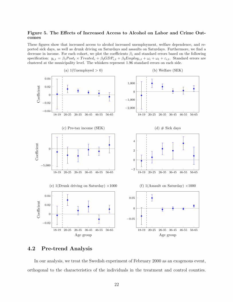
Figure 5. The Effects of Increased Access to Alcohol on Labor and Crime Out-comes

These figures show that increased access to alcohol increased unemployment, welfare dependence, and re-ported sick days, as well as drunk driving on Saturdays and assaults on Saturdays. Furthermore, we find adecrease in income. For each cohort, we plot the coefficients β1 and standard errors based on the followingspecification: yi,t = β1Postt × Treatedc + β2GDPc,t + β3Employc,t + ωi + ωt + εi,t. Standard errors areclustered at the municipality level. The whiskers represent 1.96 standard errors on each side.

18-19 20-25 26-35 36-45 46-55 56-65−0.04

−0.02

0

0.02

0.04

Coeffi

cien

t

(a) 1(Unemployed > 0)

18-19 20-25 26-35 36-45 46-55 56-65

−2,000

−1,000

0

1,000

(b) Welfare (SEK)

18-19 20-25 26-35 36-45 46-55 56-65

−5,000

0

Coeffi

cien

t

(c) Pre-tax income (SEK)

18-19 20-25 26-35 36-45 46-55 56-65−2

0

2

4

(d) # Sick days

18-19 20-25 26-35 36-45 46-55 56-65

−0.02

0

0.02

0.04

Age group

Coeffi

cien

t

(e) 1(Drunk driving on Saturday) ×1000

18-19 20-25 26-35 36-45 46-55 56-65

−0.05

0

0.05

Age group

(f) 1(Assault on Saturday) ×1000

4.2 Pre-trend Analysis

In our analysis, we treat the Swedish experiment of February 2000 as an exogenous event,

orthogonal to the characteristics of the individuals in the treatment and control counties.

22

As such, we need to test whether the variables of interest evolved in a parallel manner

in the period preceding the experiment. We provide graphical evidence in support of this

identification assumption in Figures 6 and 7. The coefficients presented in these figures were

obtained from the DDD specification in Regression (2), but we replace the Post variable

in the main interaction with a series of indicators for every other month, centered around

February 2000 (the beginning of the experiment). The coefficients reflect the difference

between treatment and control and between individuals eligible and not eligible to buy

alcohol in that particular period. We follow Brown, Grigsby, van der Klaauw, Wen, and

Zafar (2016) and perform a Wald test of the null hypothesis, that the coefficients during the

pre-period are jointly equal. Our results generally show that we cannot reject the null with

a p-value > 0.05. The Wald test results are presented in the top left corner of each chart.

Figure 6 shows the event-time evolution of the period-by-period effects of the treatment

for the number of pawn loans the individual borrowed during the 60-day period, pawn loan

size, and pawn default. The figure also shows the number of credit cards individuals own,

credit card balances, and new arrears. The Wald tests indicates that no pre-trends exist.

Figure 7 repeats this exercise for the labor market and crime results. We examine the

following labor market outcomes (annual frequency instead of every other month): an un-

employment dummy, welfare received, pretax income, and the number of sick days taken.

Again, the graphs and the associated Wald tests provide evidence consistent with the iden-

tification assumption of parallel trends. Also, Figure 7 shows the graphs for convictions for

drunk driving and assault that took place on Saturdays (Regression (3)). For both drunk

driving and assaults on Saturdays, the p-value of the Wald test confirms that we cannot

reject the parallel trends assumption in the pre-period.

4.3 Credit Market

Our analysis of the effects of the increased availability of alcohol on indebtedness ex-

plores the pawn and mainstream credit markets. Table 3 focuses on the pawn market. Odd-

23

Figure 6. Pre-Trends for Credit Outcomes

This figure lends support to our parallel growth assumption for the difference between borrowers who couldlegally purchase alcohol and those who could not in the treatment and control counties in regard to main-stream credit outcomes. The panel depicts estimates of the βτ coefficients and their 95% confidence intervalsfrom the following model: yi,t = Σt=7

t=−3βτPeriodt × Treatedc × Eligiblei,t + ξ1Treatedc × Eligiblei,t +ξ2Postt × Eligiblei,t + ξ3Eligiblei,t + ωi + ωc×t + εi,t. The x-axis shows event time, which is defined asstarting at zero in February 2000, when the Swedish government began opening liquor stores on Saturdaysin some counties. The coefficients in the pre-period are normalized at t = −2, and the respective length ofthe pre-period is determined by data restrictions. Standard errors are clustered at the municipality level.The whiskers represent 1.96 standard errors on each side.

−12 −6 0 6 12

−0.05

0

0.05

0.1

Coeffi

cien

t

(a) # New pawn loans

pWald = 0.618

−6 0 6 12

0

0.05

(b) # Credit cards

pWald = 0.960

−12 −6 0 6 12

−100

0

100

Coeffi

cien

t

(c) Pawn loan size (SEK)

pWald = 0.786

−6 0 6 12

−200

0

200

400

600

(d) Credit card balance (SEK)

pWald = 0.677

−12 −6 0 6 12−0.04

−0.02

0

0.02

Months around policy change

Coeffi

cien

t

(e) 1(Pawn loan default > 0 within 2 months)

pWald = 0.916

−6 0 6 12−0.04

−0.02

0

0.02

0.04

Months around policy change

(f) 1(Arrears > 0 within 2 months)

pWald = 0.975

24

Figure 7. Pre-Trends for Labor Market and Crime Outcomes

This figure lends support to our parallel growth assumption for the difference between borrowers who couldlegally purchase alcohol and those who could not in the treatment and control counties in regard to labormarket and crime outcomes. Panels (a) to (d) depict estimates of the βτ coefficients and their 95% confidenceintervals from the following model: yi,t = Σt=2

t=−3βτPeriodt×Treatedc×Eligiblei,t+ξ1Treatedc×Eligiblei,t+ξ2Postt×Eligiblei,t+ξ3Eligiblei,t+ωi+ωc×t+εi,t. Panels (e) and (f) depict estimates of the βτ coefficientsand their 95% confidence intervals from the following model: yi,t = Σt=8

t=−6βτPeriodt×Treatedc×Saturdayt+ξ1Treatedc × Saturdayt + ξ2Postt × Saturdayt + ξ3Saturdayt + ωi + ωd + ωc×t + εi,t. Pre-period estimatesare normalized at t = −12 for Panels (a) to (d) and at t = −2 for Panels (e) and (f). Standard errors areclustered at the municipality level. The whiskers represent 1.96 standard errors on each side.

−36 −24 −12 0 12 24

0

0.05

Coeffi

cien

t

(a) 1(Unemployed > 0)

pWald = 0.767

−36 −24 −12 0 12 24

0

2,000

4,000

(b) Welfare received (SEK)

pWald = 0.118

−36 −24 −12 0 12 24

−5,000

0

5,000

Coeffi

cien

t

(c) Pre-tax income (SEK)

pWald = 0.760

−36 −24 −12 0 12 24

−1

0

1

2

(d) # Sick days

pWald = 0.727

−12 −6 0 6 12

0

0.05

0.1

Months around policy change

Coeffi

cien

t

(e) 1(Drunk driving on Saturday) ×1, 000

pWald = 0.903

−12 −6 0 6 12

0

0.1

Months around policy change

(f) 1(Assault on Saturday) ×1, 000

pWald = 0.138

25

numbered columns present regression results from DD specifications, and the even-numbered

columns report the corresponding results from the DDD specifications. Columns (1) and (2)

show an increase in the extensive margin. Specifically, 20–25-year-olds took out more pawn

loans in the treated counties relative to peers in control countries (Column (1)) and rela-

tive to 18–19-year-olds within the same county (Column (2)). The size of the effect is the

same in both specifications and reflects an increase of 19% relative to the pre-period mean.

Columns (3) and (4) show an increase in the intensive margin, i.e., pawn loans became larger

for the treated group. The magnitude is similar, about 19–20%.

As for the performance of pawn loans, the results are mixed. We find a significant and

strong result in the DD specification (Column (5)), indicating a doubling in the number of

defaulting loans. In contrast, there is no statistically significant result in the DDD specifica-

tion (Column (6)). When considering pawn loan rollovers (Columns (7) and (8)), the point

estimates are both positive, albeit statistically significant only in Column (7).

We next explore the effects of extending the opening hours of liquor stores on the main-

stream credit market: credit cards, installment loans, and personal credit lines. In Table 4,

Columns (1)–(4) report an increase in the number of credit cards (10–11% increase) and in

the average credit card balance (12–17% increase) among the treated group. We detect no

meaningful effect on the number of installment loans and credit lines. Installment loans are

essentially credit provided when purchasing larger items, like the popular Billy bookcase and

Dombas wardrobe sold at IKEA stores. This test can be viewed as a placebo because we do

not expect the increase in alcohol availability to increase secured debt used to the finance

durable goods. We observe no change in the number of installment loans (Columns (5)

and (6)). Column (7) shows higher installment loan limits, but this result does not show up

in the DDD specification (Column (8)). The effects on credit lines are mixed: Columns (9)

and (10) show a decrease in the number of credit lines of 4% to 8%. However, Columns (11)

and (12) show an increase in the average credit balance of credit lines of about 10%.

As for credit performance, the treated group exhibits poorer performance. The likelihood

26

Table 3. Pawn Credit Outcomes

This table shows that increased access to alcohol causally increases credit borrowing and default risk.Columns (1), (3), (5), and (7) show double-difference regressions comparing individuals ages 20–25 in thetreatment counties to those in the control counties, before and after the expansion of liquor store openinghours. Columns (2), (4), (6), and (8) show regressions from DDD regressions. The sample for this analysisalso includes 18–19-year-olds, an age group ineligible to buy alcohol in Sweden. The regression is a triple-difference specification (eligible/ineligible, treatment/control, and pre/post). Standard errors are clusteredat the municipal level. *, **, and *** indicate significance at the 10%, 5%, and 1% level, respectively.

Dependent variable: # New pawn Pawn loan # Pawn loan # Pawnloans size (SEK) defaults rollovers

(1) (2) (3) (4) (5) (6) (7) (8)

Post × Treated 0.0239*** 43.23*** 0.0187** 0.00313*(0.0087) (14.67) (0.0081) (0.00159)

Post × Treated × Eligible 0.0236** 40.44 -0.00316 0.00430(0.0117) (29.63) (0.00377) (0.00435)

Post × Eligible -0.0199* -24.36 0.00433** -0.00688**(0.0105) (24.12) (0.00217) (0.00325)

Treated × Eligible -0.0155 -28.59 0.00323 -0.00668(0.0109) (21.88) (0.00292) (0.00553)

County FE Yes No Yes No Yes No Yes NoMonth FE Yes No Yes No Yes No Yes NoIndividual FE Yes Yes Yes Yes Yes Yes Yes YesAge FE Yes Yes Yes Yes Yes Yes Yes YesRegional GDP Yes No Yes No Yes No Yes NoRegional employment Yes No Yes No Yes No Yes NoCounty × Month FE No Yes No Yes No Yes No YesAges 20–25 18–25 20–25 18–25 20–25 18–25 20–25 18–25

Observations 353,264 399,178 353,264 399,178 353,264 399,178 353,264 399,178R2 0.320 0.315 0.310 0.308 0.165 0.157 0.292 0.286# Individuals 32,826 38,320 32,826 38,320 32,826 38,320 32,826 38,320

Pre-period mean 0.1233 0.1233 215.2 215.2 0.00845 0.00845 0.03708 0.03708Relative effect 19% 19% 20% 19% 221% -37% 8.4% 12%

of having any recorded arrears increases by 28% to 14% (Columns (13) and (14)).

Overall, our analysis of credit behavior shows that the treated group increased its credit

usage and experienced a deterioration in performance in both pawn and credit card instru-

ments.

27

Table

4.

Main

stre

am

Cre

dit

Outc

om

es

Th

ista

ble

show

sth

atin

crea

sed

acce

ssto

alco

hol

cau

sall

yin

crea

ses

cred

itb

orro

win

gan

dd

efau

ltri

sk.

Th

eod

d-n

um

ber

edco

lum

ns

show

dou

ble

-d

iffer

ence

(DD

)re

gres

sion

sco

mp

arin

gin

div

idu

als

ages

20–2

5in

the

trea

tmen

tco

unti

esto

thos

ein

the

contr

olco

unti

es,

pre

and

pos

tth

eex

pan

sion

inop

enin

gh

ours

:y i,t

=β1Post t×Treatedc

+β2GDPc,t

+β3Employ c,t

+ωi+ωt+ε i,t

.T

he

even

-nu

mb

ered

colu

mn

ssh

owre

sult

sfr

omtr

iple

-diff

eren

ce(D

DD

)re

gres

sion

s:y i,t

=β1Post t×Treatedc×Eligiblei,t+β2Post t×Treatedc

+β3Post t×Eligiblei,t+β4Eligiblei,t+ωi+ωc×t+ε i,t.

Th

esa

mp

lefo

rth

isan

alysi

sal

soin

clu

des

18–1

9-yea

r-ol

ds,

an

age

grou

pin

elig

ible

tob

uy

alco

hol

inS

wed

en.

Sta

nd

ard

erro

rsar

ecl

ust

ered

atth

em

un

icip

al

leve

l.*,

**,

and

***

ind

icat

esi

gnifi

cance

at

the

10%

,5%

,an

d1%

leve

l,re

spec

tivel

y.

Dep

enden

tva

riab

le:

Cre

dit

card

s#

Inst

allm

ent

Inst

allm

ent

Cre

dit

lines

#C

redit

card

sbal

ance

(SE

K)

loan

slim

it(S

EK

)#

Cre

dit

lines

bala

nce

(SE

K)

1(A

rrea

rs>

0)

(1)

(2)

(3)

(4)

(5)

(6)

(7)

(8)

(9)

(10)

(11)

(12)

(13)

(14)

Pos

t×

Tre

ated

0.01

97**

*11

7.8*

**-0

.001

113

9.2*

**-0

.011

8***

328.6

***

0.0

151***

(0.0

033)

(24.

4)(0

.001

4)(4

8.2)

(0.0

030)

(84.8

)(0

.0057)

Pos

t×

Tre

ated×

Eligi

ble

0.02

27**

*16

5.7*

**-0

.001

910

.8-0

.0247***

336.3

***

0.0

075*

(0.0

050)

(47.

0)(0

.001

3)(6

4.8)

(0.0

064)

(121.9

)(0

.0045)

Pos

t×

Eligi

ble

-0.0

035

-72.

9***

0.00

35**

*13

0.6*

*0.0

027

50.2

0.0

086***

(0.0

032)

(26.

5)(0

.001

2)(5

4.2)

(0.0

056)

(81.9

)(0

.0032)

Tre

ated×

Eligi

ble

-0.0

191*

**-8

7.5

0.00

93**

224.

1*0.0

180

-404.3

*-0

.0140*

(0.0

073)

(74.

8)(0

.004

7)(1

22.0

)(0

.0113)

(239.7

)(0

.0074)

Cou

nty

FE

Yes

No

Yes

No

Yes

No

Yes

No

Yes

No

Yes

No

Yes

No

Mon

thF

EY

esN

oY

esN

oY

esN

oY

esN

oY

esN

oY

esN

oY

esN

oIn

div

idual

FE

Yes

Yes

Yes

Yes

Yes

Yes

Yes

Yes

Yes

Yes

Yes

Yes

Yes

Yes

Age

FE

Yes

Yes

Yes

Yes

Yes

Yes

Yes

Yes

Yes

Yes

Yes

Yes

Yes

Yes

Reg

ional

GD

PY

esN

oY

esN

oY

esN

oY

esN

oY

esN

oY

esN

oY

esN

oR

egio

nal

emplo

ym

ent

Yes

No

Yes

No

Yes

No

Yes

No

Yes

No

Yes

No

Yes

No

Cou

nty×

Mon

thF

EN

oY

esN

oY

esN

oY

esN

oY

esN

oY

esN

oY

esN

oY

es

Obse

rvat

ions

233,

287

261,

905

233,

287

261,

905

233,

287

261,

905

233,

287

261,

905

233,

287

261,9

05

233,2

87

261,9

05

233,1

39

261,7

48

R2

0.89

70.

897

0.76

10.

760

0.78

30.

782

0.76

60.

765

0.82

80.8

26

0.8

30

0.8

30

0.4

35

0.4

35

#In

div

idual

s29

,416

34,9

0229

,416

34,9

0229

,416

34,9

0229

,416

34,9

0229

,416

34,9

02

29,4

16

34,9

02

29,3

72

34,8

52

Pre

-per

iod

mea

n0.

208

0.20

895

1.2

951.

20.

046

0.04

61,

209

1,20

90.

328

0.3

28

3,4

88

3,4

88

0.0

55

0.0

55

Rel

ativ

eeff

ect

9.5%

11%

12%

17%

-2.4

%-4

.1%

12%

0.9%

-3.6

%-7

.6%

9.4

%9.6

%28%

14%

28

4.4 Monday Borrowing

To provide further corroborating evidence about the causal relation between the increased

availability of alcohol and indebtedness, we take advantage of the high-frequency nature of

the pawn registry. The impromptu consumption of alcohol on Saturdays causes individuals

in the treated counties to be more likely to hit an unexpected liquidity shortage over the

weekend. However, since pawn shops were closed over the weekends in the early 2000s, the

liquidity shortage would translate into borrowing once pawn shops opened, on Monday.

We construct a person-date data set in which we record the number of pawn loans that

each person took on a particular date (typically zero or one). Table 5, Columns (1) and (3)

show the baseline regression results (DD and DDD, respectively). In Columns (2) and (4),

we explore whether there was an uptick in pawn borrowing activity on Mondays in counties

exposed to greater availability of alcohol. We interact the variable of interest with a Monday

indicator and add day-of-the-week dummies to absorb the average tendency to borrow on

a certain day. The table shows that 24–27% of the increase in pawn borrowing due to the

treatment takes place on Mondays.17

In summary, the results in Table 5 indicate a disproportionate increase in borrowing

on Mondays among the treated group, consistent with the idea that the extended opening

hours on the weekend generated “unexpected” negative shocks to consumers with present-

focused preferences. A rational consumer would be able to avoid the liquidity shortage on

the weekend as she would plan the purchase and would borrow ahead of time, if needed.

4.5 Multiplier Effect of Alcohol Consumption

We next assess whether the increased availability of alcohol among the treated population

impacted individuals beyond the higher spending on alcohol, i.e., caused additional expen-

diture or financial consequences. For example, consumption of alcohol may be associated

17We calculate the 24–27% increase on Mondays in the following manner: (average daily effect + averageeffect on Monday)/((5× average daily effect) + average effect on Monday)) = (0.00047 + 0.00013)/((5 ×0.00047) + 0.00013)) = 24%. A similar calculation using the coefficients in Column (4) yields 27%.

29

Table 5. Weekly Pattern of Pawn Credit Borrowing

This table tests whether pawn borrowing in the treatment group was more likely to take place on Mondays.The sample is at the person-day level and covers the years 1999 to 2001. Columns (1) and (2) show resultsfrom the double-difference (DD) regressions comparing individuals ages 20–25 in the treatment counties tothose in the control counties, before and after the expansion of liquor store opening hours: yi,t = β1Postt ×Treatedc × 1(Mondayt) + β2Postt × Treatedc + β3GDPc,t + β4Employc,t + ωi + ωt + εi,t. Columns (3)and (4) show results from triple-difference (DDD) regressions. The sample for this analysis also includes18–19-year-olds, an age group ineligible to buy alcohol in Sweden. The regression is a DDD specification(eligible/ineligible, treatment/control, and pre/post): yi,t = β1Postt×Treatedc×Eligiblei,t×1(Mondayt)+β2Postt×Treatedc+β3Postt×Eligiblei,t+β4Eligiblei,t+ . . . 1(Mondayt) interactions . . .+ωi+ωc×t+εi,t.1(Monday) is a dummy variable that is equal to one if the pawn loan was taken on a Monday and zerootherwise. For this exercise, we use our panel at a daily frequency. The data include borrower-calendarday observations in which we count the number of pawn loans that were taken in every calendar day of theweek (typically zero or one). Standard errors are clustered at the individual level. *, **, and *** indicatesignificance at the 10%, 5%, and 1% level, respectively.

Dependent variable: # New pawn loans

(1) (2) (3) (4)

Post × Treated 0.00050** 0.00047**(0.00021) (0.00018)

Post × Treated × 1(Monday) 0.00013(0.00016)

Post × Treated × Eligible 0.00036 0.00033(0.00040) (0.00039)

Post × Treated × Eligible × 1(Monday) 0.00015*(0.00016)

1(Monday) 0.00060*** 0.00057***(0.00007) (0.00006)

Post × Eligible -0.00040 -0.00042*(0.00025) (0.00025)

Treated × Eligible -0.00043 -0.00043(0.00034) (0.00034)

Weekday FE No Yes No YesCounty FE Yes Yes No NoCalendar month FE Yes Yes No NoIndividual FE Yes Yes Yes YesAge FE Yes Yes Yes YesRegional GDP Yes Yes No NoRegional employment Yes Yes No NoCounty × Calendar month FE No No Yes Yes

Observations 16,866,840 16,866,840 19,088,938 19,088,938R2 0.015 0.015 0.015 0.015# Individuals 37,824 37,824 44,071 44,071Sample period 1999–2001 1999–2001 1999–2001 1999–2001Ages 20–25 20–25 18–25 18–25

30

with additional purchases, road accidents, or loss of income.

To calculate the multiplier effect of alcohol consumption, we must first determine the

increase in spending on alcohol that occurred when liquor store opening hours were expanded

and then compare that figure to the observed increase in credit usage. The increase in

alcohol expenditure can be estimated using past studies of alcohol consumption patterns

in Sweden as well as the studies that analyzed the opening hours experiment. Statistics

Sweden (Statistiska centralbyran) collects expenditure information for various items using

cash journals distributed to a sample of individuals. We use the data covering expenditure

information by 4,688 people for the years 1999–2001. The average annual spending on alcohol

is provided in Online Appendix Table A5. The table shows that the average spending on

alcohol among young people in the lowest income group (likely to be the population in our

main sample) was about 2,800 SEK (about $280) a year.18 Thus, an increase of 4% in their

drinking translates into an increase of 112 SEK per capita per year for people in the 20–25

age cohort.19 We obtain similar figures if we rely on aggregate data.20

Now, compare this estimation to our finding in Tables 3 and 4 that, on average, people

ages 20–25 living in the treated counties increased their total debt balance by about 502 SEK

18These figures could be compared to a similar study done in the U.S. in 2001 (https://www.bls.gov/cex/csxann01.pdf). Individuals in the lowest income quintile spend $220 per year on alcohol, relative tothe average consumption of $349. Individuals in the 20–25 age range spent $368 per year, on average.

19We do not observe individuals’ change in alcohol consumption directly and therefore make the assumptionthat the increase in alcohol expenditure for the young is equal to the average increase in alcohol sales forthe population (see estimations by Norstrom and Skog, 2003; Gronqvist and Niknami, 2014). If, however,individuals ages 20–25 increased their alcohol expenditure by more than the average person in the populationdid, then the multiplier that we calculate would be lower (and would be closer to the estimation by Schilbach,2019). It is unclear whether the larger effect that we find for the young relative to older cohorts (e.g., onindebtedness) is generated by a larger increase in spending on alcohol or by the fact that they are likely to becloser to their liquidity constraint than older cohorts. If indeed young people have a stronger consumptionresponse to the availability of alcohol, then the 4.5 multiplier estimate is likely to be an upper bound of themultiplier.

20The total revenue from off-premise alcohol sales in Sweden in 2000 was 17.368 billion SEK (source: his-torical trends in Systembolaget’s Responsibility Report for 2008). Norstrom and Skog (2005) and Gronqvistand Niknami (2014) report an increase in alcohol sales of 4%. The increase in sales translates to about277 to 299 million SEK in additional sales, assuming that the increase in sales is spread over 43% of thetransactions, corresponding to the fraction of the population in the treatment areas. In 2000, the Swedishpopulation in the treatment counties was 3.822 million (Figure 1), approximately 75% of whom were between20 and 80 years old, the population likely to drink (see https://www.cia.gov/library/publications/

the-world-factbook/geos/sw.html). Hence, the average increase in alcohol consumption per capita inthe treatment counties was 97 to 104 SEK per capita per year (330m SEK/(3.822m × 75%)).

31

(about $50).21 Comparing this amount to the estimated amount spent on alcohol of 112 SEK

suggests a multiplier effect of 4.5, which is consistent with the idea that increased alcohol

consumption leads to poor decision making on other dimensions such as driving under the

influence (Wagenaar et al., 2000; Levitt and Porter, 2001), lack of savings (Schilbach, 2019),

or loss of income or jobs, as we report here. This figure is twice as large as the magnitude

of the multiplier that Schilbach (2019) reports in the population of Indian rickshaw drivers,

though, of course, the populations in the two studies are different (Indian cab drivers versus

Swedish young people) with differential access to credit. For example, Swedes are able to

borrow through credit cards and thus may be able to increase consumption more easily in

response to greater availability of alcohol compared to Indian cab drivers.

This estimate reflects a lower bound for both the average effect across the population

and for those who suffer from present-focused preferences. The increase in debt balances

is estimated using the accounts of all 20–25-year-olds. Our measurement of the effects are

based on debt balances. However, some individuals may finance their consumption through

other sources, e.g., available cash. When we split the sample by financial constraints, the

effect increases by 50% to about 750 SEK, on average, for the group that we identify as more

financially constrained (see Table 8 discussed in more detail in Section 5.1).

It is useful to quantify the impact of the increase in debt balance by examining it relative

to their income. An increase of 502 SEK in their revolving credit balance is equivalent to a

10.5% increase relative to their pre-experiment mean outstanding debt balance and 7.1% of

their pre-mean monthly disposable income.22

The increase in debt balances also reinforces the explanatory mechanism—present-focused

preferences. Specifically, since the increase in access to alcohol resulted in an additional high-

interest debt, the interest rate on this debt could be a lower-bound estimate for the discount

21The credit balance of the DDD is 165.7 SEK (credit cards) + 336.3 SEK (credit lines) = 502 SEK totalincrease in credit. The pre-period mean of the treated counties = 951 SEK (credit cards) + 3,488 SEK(credit lines) = 4,439 SEK total pre-period mean. Thus, the relative increase for the treated population20–25-year-olds = 502/4,439 = 11.3%.

22The mean annual disposable income is 85,355 SEK for the 20–25-year-olds living in the treatmentcounties, measured in the pre-period. Then, 85,355/12 = 7,113 SEK/month; 502/7,113 = 7.1%.

32

rate of individuals. Our data do not allow us to directly observe the annualized percentage

rate (APR) paid on the different credit instruments; however, it is well known that the APR

for unsecured consumer debt was, and still is, over 20%. Hence, the implicit discount rate

that individuals use when trading off current and future consumption must be higher than

this figure.

In addition to the direct trade-off, there are less salient indirect costs that are especially

deleterious for the individuals we study who are situated at the margins of the formal credit

and labor market. These costs are generated by the increase in default risk. We find that the

probability of receiving a new arrear within the next 12 months increases by 0.07 percentage

points, which is an increase of 14% relative to their pre-experiment mean. These arrears

will remain on the individuals’ credit register for three years after the debt has been repaid.

From the literature, we know that negative information on an individual’s’ credit register not

only worsens his or her credit access,23 but also can lead to costly labor market exclusion.

These effects on employment and earnings are four times larger than the effects on credit

(Bos, Breza, and Liberman, 2018).

4.6 Labor Market

Our results thus far indicate that increased availability of alcohol leads to greater indebt-

edness by a magnitude greater than the pure increase in spending on alcohol. One channel

through which alcohol could cause greater indebtedness is the labor market, where individ-

uals’ performance may deteriorate, causing them to lose income. We explore this channel

by using annual employment and wage information from the Swedish tax authority, filed by

all Swedish residents beginning at age 18. As tax filings are annual in frequency and the

experiment started in the middle of 2000, we examine effects in both 2000 and 2001, and

23See for example, Musto (2004), Brown and Zehnder (2007); Djankov, McLiesh, and Shleifer (2007), Bosand Nakamura (2014), Liberman (2016), and Dobbie, Goldsmith-Pinkham, Mahoney, and Song (2016).

33

compare them to the pre-period of 1996 to 1999.24

Table 6. Labor Market Outcomes

This table shows that increased access to alcohol causally increases credit borrowing and default risk.Columns (1), (3), (5), and (7) show results from the following double-difference (DD) regression comparingindividuals ages 20–25 in the treatment counties to those in the control counties, before and after the ex-pansion of liquor store opening hours: yi,t = β1Postt× Treatedc + β2GDPc,t + β3Employc,t +ωi +ωt + εi,t.Columns (2), (4), (6), and (8) show results from triple-difference (DDD) regressions. The sample for thisanalysis also includes 18–19-year-olds, an age group ineligible to buy alcohol in Sweden. The regressionis a DDD specification (eligible/ineligible, treatment/control, and pre/post): yi,t = β1Postt × Treatedc ×Eligiblei,t + β2Postt × Treatedc + β3Postt × Eligiblei,t + β4Eligiblei,t + ωi + ωc×t + εi,t. Standard errorsare clustered at the municipal level. *, **, and *** indicate significance at the 10%, 5%, and 1% level,respectively.

Dependent variable: 1(Unemployed) Welfare Pre-tax income #Sick days

(1) (2) (3) (4) (5) (6) (7) (8)

Post × Treated 0.0146 1,019* -1,886 0.579(0.0097) (522.0) (2,451) (1.249)

Post × Treated× Eligible 0.0110 1,917*** -1,530 0.0711(0.0229) (659.2) (1,617) (0.732)

Treated× Eligible -0.0126 -1,717*** 676.5 1.089(0.0089) (356.8) (1,321) (0.668)

Post × Eligible -0.0029 -1,164** 697.7 0.0775(0.0104) (481.7) (1,218) (0.574)

County FE Yes No Yes No Yes No Yes NoCalendar Year FE Yes No Yes No Yes No Yes NoIndividual FE Yes Yes Yes Yes Yes Yes Yes YesAge FE Yes Yes Yes Yes Yes Yes Yes YesRegional GDP Yes No Yes No Yes No Yes NoRegional employment Yes No Yes No Yes No Yes NoCounty × Year FE No Yes No Yes No Yes No YesAges 20–25 18–25 20–25 18–25 20–25 18–25 20–25 18–25

Observations 135,480 175,924 136,382 177,012 136,382 177,012 135,480 175,924R2 0.622 0.584 0.701 0.659 0.738 0.701 0.569 0.508# Individuals 42,087 47,986 42,204 48,076 42,204 48,076 42,087 47,986

Pre-period mean 0.5679 0.5679 12,918 12,918 64,258 64,258 5.523 5.523Relative effect 2.6% 1.9% 7.9% 15% -2.9% -2.4% 10% 1.3%

Next, we conduct formal tests using both DD and DDD specifications for the 18–19 and

24The effects in the labor market could be either direct or indirect. Prior research has documented a directchannel of alcohol consumption resulting in reduced workplace productivity (e.g., Blum et al., 1993; Joneset al., 1995; Fisher et al., 2000; McFarlin and Fals-Stewart, 2002). There is also an indirect channel: Adefault flag on one’s credit record could hurt the likelihood of being hired by potential employers who checkcredit records (e.g., Balance, Clifford, and Shoag, 2016; Bartik and Nelson, 2019; Cohen-Cole, Herkenhoff,and Phillips, 2016; Bos et al., 2018). In the current empirical setting, we cannot discriminate between thetwo channels.

34

20–25 cohorts. In Table 6, we use the following dependent variables: likelihood of being

unemployed, welfare receipts, pretax income, and the number of sick days taken. Aside

from the lower frequency of observations, the empirical specification is identical to that used

in previous tables. The odd and even columns, respectively, present results from DD and

DDD specifications. In general, the effects of the expanded opening hours on labor market

outcomes are negative, albeit weak. All coefficient signs are in the expected direction, but

only the welfare results (Columns (3) and (4)) are statistically significant.

Overall, we find modest, yet existent, effects in the labor market for the treated group.

The effects might be small and estimated with noise because of the low (annual) frequency

and the indirect channel.

4.7 Reckless Behavior: Evidence from Crime Records

The behavioral sciences literature has found a tight relation between alcohol availability,

consumption, and the propensity to commit crime, perhaps because alcohol consumption

impairs judgment and can prompt violent actions (McClelland, Davis, Kalin, and Wanner,

1972; Gliksman and Rush, 1986; Rush, Gliksman, and Brook, 1986).

To explore whether this relation holds for the individuals in our sample, we analyze

their incidence rate of crimes related to alcohol consumption. We first look at the effects for

different age cohorts. In Figure 5, we plot the DDD coefficients measuring upticks in criminal

activity on Saturdays among the treated group from Regression (3) for the six age groups.

As expected, the charts show no significant increase in alcohol-related crimes on Saturdays

for the cohort of 18–19-year-olds. Assaults and drunk driving on Saturdays do, however,

increase among 20–25-year-olds, who are eligible to purchase alcohol. This finding is in line

with our previous result that the largest increase in indebtedness was among 20–25-year-olds

(Section 4.3).

35

Table

7.

Eff

ect

of

Liq

uor

Sto

res

Bein

gO

pen

on

1(S

atu

rday)

Cri

me

Th

ista

ble

test

sw

het

her

incr

ease

dac

cess

toal

coh

olin

crea

ses

the

risk

for

crim

eson

Sat

urd

ays.

Col

um

ns

(1)

and

(6)

show

the

regr

essi

on

:y i,t

=β1Post t×Treatedi

+β2Post t×Treatedc

+ωi

+ωd

+ωc×t

+ε i,t

.C

olu

mn

s(2

)–(4

)an

d(7

)–(9

)sh

owth

ere

gres

sion

:y i,t

=β1Post t×Treatedi×

1(Saturday t

)+β2Post t×Treatedc

+β3Post t×

1(Saturday t

)+ωi+ωd

+ωc×t+ε i,t

.C

olu

mn

s(5

)an

d(1

0)sh

owtr

iple

-diff

eren

ce(D

DD

)re

gre

ssio

ns

esti

mat

ing

Reg

ress

ion

(3).

Dep

end

ent

vari

able

:1(

Ass

ault>

0)×

1000

1(D

run

kd

rivin

g>0)×

1000

(1)

(2)

(3)

(4)

(5)

(6)

(7)

(8)

(9)

(10)

Pos

t×

Tre

ated

0.00

92-0

.002

8(0

.006

7)(0

.002

9)P

ost×

Tre

ated×

1(S

atu

rday

)0.0

497*

**0.

0867

***

0.00

230.

0308

**0.

0577

***

-0.0

037

(0.0

161)

(0.0

313)

(0.0

089)

(0.0

121)

(0.0

221)

(0.0

033)

Pos

t×

1(S

atu

rday

)-0

.043

7***

-0.0

728*

**-0

.005

4-0

.023

2***

-0.0

436*

**0.

0038

*(0

.013

1)(0

.025

5)(0

.007

5)(0

.008

9)(0

.015

9)(0

.002

3)T

reat

ed×

1(S

atu

rday

)-0

.022

5-0

.036

8-0

.001

1-0

.013

1-0

.023

50.

0025

(0.0

148)

(0.0

275)

(0.0

083)

(0.0

101)

(0.0

184)

(0.0

018)

Pos

t×

Tre

ated×

Eli

gib

le0.

0273

**-0

.0053

(0.0

115)

(0.0

078)

Pos

t×

Eli

gib

le-0

.022

6***

0.0

080

(0.0

080)

(0.0

057)

Tre

ated×

Eli

gib

le0.

0231

-0.0

062

(0.0

165)

(0.0

098)

Cou

nty

FE

Yes

Yes

Yes

Yes

Yes

Yes

Yes

Yes

Yes

Yes

Yea

rF

EY

esY

esY

esY

esY

esY

esY

esY

esY

esY

esIn

div

idu

alF

Ean

dA

geF

EY

esY

esY

esY

esY

esY

esY

esY

esY

esY

esR

egio

nal

GD

PY

esY

esY

esY

esN

oY

esY

esY

esY

esN

oR

egio

nal

emp

loym

ent

Yes

Yes

Yes

Yes

No

Yes

Yes

Yes

Yes

No

Day

ofW

eek

FE

Yes

Yes

Yes

Yes

Yes

Yes

Yes

Yes

Yes

Yes

Cou

nty×

Yea

rF

EN

oN

oN

oN

oY

esN

oN

oN

oN

oY

esA

ges

20–2

520

–25

20–2

520

–25

20–2

518

–25

20–2

520

–25

20–2

518–25

Gen

der

All

All

Mal

eF

emal

eA

llA

llA

llM

ale

Fem

ale

All

Ob

serv

atio

ns

20,7

02,5

1820,

702,

518

11,3

46,5

869,

355,

932

23,4

09,4

7220

,702

,518

20,7

02,5

1811

,346

,586

9,35

5,93

223,4

09,4

72

#In

div

idu

als

32,6

6732

,667

17,8

7414

,793

38,1

4332

,667

32,6

6717

,874

14,7

9338,1

43

Pre

-mea

n0.

0302

0.0

580.

0976

0.01

120.

0302

0.01

390.

0322

0.05

720.

0028

10.0

139

Rel

ativ

eeff

ect

31%

86%

89%

20%

90%

-20%

96%

101%

-130

%-3

8%

36

Our data set contains the exact date of the crime;25 therefore, we can test whether crimes

increased more on Saturdays relative to the other days of the week in the treated counties

and in the post-period. This detailed identification strategy is taken from Yoruk and Lee

(2018), who find an increase in crime rates in the U.S. on Sundays (but not on other days)

following the legalization of Sunday alcohol sales. For this purpose, we construct a data set

at the daily frequency and run Regression (3).

The results in Columns (2) and (7) of Table 7 confirm that the treated counties saw

a statistically significant increase in assaults and drunk driving on Saturdays during the

post-period. For this population, the likelihood of assaults on Saturdays in the treatment

counties increased by 0.0050 percentage points (relative to the pre-period mean of 0.0058

percentage points). Similarly, the likelihood of drunk driving on Saturdays increased by

0.0031 percentage points, an increase of 95% relative to the pre-period mean in the treatment

counties of 0.0032 percentage points. Columns (3)–(4) and (8)–(9) show that these results are

completely driven by young males, which is consistent with the crime literature mentioned

above.

Overall, this evidence corroborates our previous results on two fronts. First, these find-

ings are consistent with the idea that weekend drinking increased when liquor store oper-

ating hours expanded. Second, these results suggest that individuals may have had more

unplanned expenditures because of increased alcohol consumption stemming from greater

access to alcohol on Saturdays.

5 Supplementary Results

In this section, we provide supplementary results to our main analysis. First, we explore

the role of liquidity constraints in the decision making of the young cohort. Second, we test

whether the demand for credit was concentrated in a small part of the population (a few

25In some cases, such as break-ins, the exact day of the crime may be unknown. In these cases, the courtassigns a date based on an educated guess. However, because no ambivalence exists about the exact date ofan assault or drunk driving, our results do not suffer from this error.

37

alcohol addicts) or whether it was spread across the treated population. Third, we explore

the possibility of an alternative explanation for our results based on the idea of latent demand

for alcohol, i.e., that weekend opening hours enabled busy (yet rational) people to visit liquor

stores. Finally, we conduct several robustness tests of our main results in Online Appendix

C. These include excluding border counties, a permutation (placebo) test, and running our

analysis at the aggregated county level.

5.1 The Role of Liquidity Constraints

As we saw in the earlier analysis, the young cohorts increase consumption more than

older cohorts due to drinking patterns (Figure 3). Still, liquidity constraints—which are

likely to be more acute for young people (e.g., Hayashi, 1985)—could intensify the response

of the young, especially because young people had little opportunity to accumulate liquidity.

We test this hypothesis by focusing on the 20–25 cohort, and splitting them by a proxy

for liquidity constraints, i.e., having a below-the-median bank account balance. We follow

Calvet, Campbell, and Sodini (2007) and Calvet and Sodini (2014) and impute the bank

account balances based on the subsample of individuals (about 250,000) in the wealth data

for which bank account balances are observed even though the earned interest is less than

100 SEK.26 This way, we hold age constant and vary liquidity.

The results of this test, in Table 8, show that the impact of the opening hours experiment

is concentrated in the below-median liquidity group. It is important to note that while

we can directly measure the impact on the alcohol expenditure per age cohort, we cannot

directly pinpoint the causal link between lack of liquidity and the negative impacts of alcohol

expenditure. We can say, however, that there is an effect that is correlated with liquidity

beyond simply the age effect.

26The observed balance is regressed onto the following observable characteristics: age and squared ageof the household head, household size, real estate wealth, level and squared level of household disposableincome, and financial wealth other than bank accounts. The coefficients from this regression are then usedto impute the account balances of individuals who report no bank account. Note that the fraction of Swedesages 15 years and above who have a bank account has been reported to be 99% (Honohan, 2008).

38

Table 8. DDD Regressions: Sample Splits Based on Imputed Bank Liquidity

The table presents the DDD estimations for the main variable of interest in the original sample as well as intwo subsamples based on their imputed bank balance: Illiquid (below-the-median) and Liquid (above-the-median). Standard errors are clustered at the municipality level. *, **, and *** indicate significance at the10%, 5%, and 1% level, respectively.

Sample: Original Illiquid Liquid Original Illiquid Liquid

(1) (2) (3) (4) (5) (6)

# New pawn loans Pawn loan value

Post × Treated × Eligible 0.024** 0.057*** -0.005 40 71* 17(0.012) (0.018) (0.014) (30) (38) (30)

# Individuals 38,320 18,134 18,183 38,320 18,134 18,183

Pawn default # Credit cards

Post × Treated × Eligible -0.003 -0.004 -0.004 0.023*** 0.031*** 0.016**(0.004) (0.005) (0.005) (0.005) (0.005) (0.007)

# Individuals 38,320 18,134 18,183 34,902 16,738 16,305

Credit cards balance Credit lines balance

Post × Treated × Eligible 166*** 266*** 87* 336*** 481*** 241(47) (73) (48) (122) (171) (152)

# Individuals 34,902 16,738 16,305 34,902 16,738 16,305

Welfare (SEK) Pre-tax income (SEK)

Post × Treated × Eligible 1,917*** 2,279*** 1,393 -1,530 -2,265 -224(659) (650) (905) (1,617) (2,367) (2,964)

# Individuals 48,076 23,301 23,610 48,076 23,301 23,610

Individual FE and Age FE Yes Yes Yes Yes Yes YesCounty × Time FE Yes Yes Yes Yes Yes Yes

Drunk driving Assault

Post × Treated × Saturday 0.031*** 0.029* 0.034 0.050*** 0.119*** -0.013(0.012) (0.015) (0.021) (0.016) (0.022) (0.024)

# Individuals 32,667 15,545 15,545 32,667 15,545 15,545

County FE Yes Yes Yes Yes Yes YesCalendar month FE Yes Yes Yes Yes Yes YesIndividual FE and Age FE Yes Yes Yes Yes Yes YesRegional GDP Yes Yes Yes Yes Yes YesRegional employment Yes Yes Yes Yes Yes YesDay of the week FE Yes Yes Yes Yes Yes Yes

39

5.2 A Few Alcoholics? The Distribution of Borrowers

The results so far have shown an increase in the average demand for credit. An important

question is whether this increase is evenly spread across the population or is skewed. A

skewed distribution would suggest that a small number of people (potentially alcoholics) are

driving the results. Conversely, an even distribution would indicate that the effect is spread

throughout the population.

In contrast to our previous analyses in which we estimated the average effect, here our

objective is to examine the distribution of the effect across individuals. We rerun Regres-

sion (2) but exclude the triple interaction. This exclusion adds this demeaned variable to the

residual, allowing us to examine the distribution of the effects for individuals in the treat-

ment group. We focus on the subset of individuals who actually borrowed and ask whether

the positive increase in loan size among the treated group is driven by a small number of

large loans or by across-the-board borrower demand.

Figure 8. Distribution of Residuals of Loan Sizes and Balances in the TreatmentCounties

The charts plot the distribution of the residuals for pawn loan size and credit card balance for the treatmentcell, i.e., Post × Treated × Eligible, from the baseline specification (Regression (1)) without the triple-interaction: yi,t = β1Postt × Treatedc + β2Postt ×Eligiblei,t + β3Eligiblei,t + ωi + ωc×t + εi,t. The sampleused in Panel (a) includes all individuals who took a pawn loan. The sample used in Panel (b) includes allindividuals who have a credit card.

−4−3−2−1 0 1 2 3 4 5 6 7 8 9 10

0

0.1

0.2

0.3

Loan size (residual; ’000 SEK)

Fre

qu

ency

(a) Residuals of pawn loan size

−12−9−6−3 0 3 6 9 12 15 18 21 24

0

0.1

0.2

0.3

Credit card balance (residual; ’000 SEK)

(b) Residuals of credit card balance

The charts in Figure 8 show the distribution of the residuals of the loan sizes of pawn

and credit card borrowers. In both charts, the distribution of the borrowing is concentrated

40

in a single cluster, with no material outliers. We conclude that the increase in borrowing in

the treated counties is not driven by a small part of the population but rather is relatively

dispersed.

5.3 Present-Focused Preferences or Convenience Shopping?

So far, we have documented an economically large cost to the increase in access to alcohol

among individuals at the margins of the formal credit markets. We explained the effect as

a response among consumers with impulsive consumption behavior to the wider availability

of alcohol.

Another, non-mutually exclusive, explanation is possible. The extended opening hours

could make purchasing alcohol more convenient and thus may reveal latent demand among

busy consumers. As a result, both consumption of alcohol and reliance on credit would

increase. If this were true, even with a fully rational population, we would observe an

increase in alcohol purchases and higher use of credit in the counties where liquor stores

are open on Saturdays. The Saturday opening hours may simply allow people with busy

weekday schedules to purchase alcohol. Thus, according to this narrative, the Saturday store

opening hours represent a reduction in opportunity costs.

The ideal test—randomly assigned leisure—does not exist in our data. However, we iden-

tify two subgroups—retirees and the unemployed—for whom the convenience benefit from

opening the stores on Saturdays is endogenously minimal. If retirees and the unemployed

indeed do not have present-focused preferences, then they can execute their plan to purchase

alcohol during the week with no inconvenience and consume the alcohol over the weekend,

even if the stores are closed on Saturdays. In other words, opening the liquor store on

Saturdays should not affect their behavior. Saturday opening hours should affect rational

individuals who work during the week. Therefore, if the effects that we document are due to

increased convenience, then we should find a large difference in the financial consequences

for employed individuals relative to those who are not working.

41

We test this hypothesis in Online Appendix Tables A6 and A7. The tables contrast the

financial effects for retirees (ages 65–75) versus older employees (ages 55–60), and unemployed

versus employed individuals (both in the 20–65 age range). Because the comparison with

18–19-year-olds is no longer appropriate, we run a DDD specification in which the final

difference is a dummy for being retired or unemployed.27

The results reveal little difference in the financial outcomes of the employed population

and those with more flexible schedules. These non-results are not driven by low power (these

samples are large: 267,000 to 1,296,000 observations), but rather by coefficients that are close

to zero with tight standard errors. For example, in Columns (1) and (2) of Online Appendix

Table A6, we estimate the effect on the number of new pawn loans. The coefficients are

−0.002 and −0.016 for retirees and the unemployed, respectively, with standard errors of

0.008 and 0.014. In comparison, in Table 3, Columns (1) and (2), the coefficients are 0.024.

Similarly, in Online Appendix Table A7, we estimate the effect on the number of credit

cards. The coefficients are 0.005 and 0.011 for retirees and the unemployed, respectively,

with standard errors of 0.011 and 0.009. In comparison, in Table 4, Columns (1) and (2),

the coefficients are 0.020 and 0.023, respectively.

These results suggest that busier populations did not borrow more following the exten-

sion of opening hours on Saturdays. This result is consistent with the idea that alcohol

is a temptation good that triggers present-biased behavior in people and leads to current

consumption at the expense of future consumption.

6 Discussion

Our results have important implications for the lives of poor individuals living in wealthy

countries. Our study measures the effects of extending the opening hours of liquor stores,

which is effectively a relaxation of a commitment device that prevented impulsive consump-

27One caveat is that the power of the retiree test might not be high, given that this age group might notbe very susceptible to the increase in alcohol availability (see Figures 4 and 5).

42

tion prior to the extension of the operating hours.

Two main theories link present-focused preferences to poverty, and both conclude that

the value of (and therefore the demand for) commitment devices is highest among the poor.

In Banerjee and Mullainathan (2010), while all people are equally sensitive to impulsive

consumption, poor people have lower ability to absorb the adverse costs of impulsive con-

sumption due to lack of a financial buffer. In Bernheim et al. (2015), individuals are endowed

with different levels of present-focused preferences. People with severe present-focused pref-

erences deplete their assets quickly and become poor. Because they are poor, they have

lower ability to punish themselves for deviating from their planned consumption path, and

therefore are more likely to cave in to impulsive consumption.

Through its policies, the government can institute commitment devices that can help

poor individuals improve their financial wellbeing. One particular way that the government

can intervene is by limiting the opportunities for impulsive consumption. Restricting the

opening hours of alcohol stores over the weekend is one such policy.

In practice, however, governments may choose to avoid instituting commitment devices—

restrictive access to temptation goods, in our case—for two reasons. First, while enabling

free access to temptation goods induces costs due to impulsive consumption, it might also

create value by offering more flexible shopping options and hence convenience. Alluding to

this tradeoff, Systembolaget’s CEO Anitra Steen says in an interview (February 5, 2000,

right before the initiation of the nationwide experiment): “The Parliament believes that our

legitimacy with the Swedish people must be strengthened in order to guarantee the long-term

survival of Systembolaget. One way to do that is to open on Saturdays and thus improve the

service to the customers.”28 Second, the costs of impulsive consumption are disproportion-

ately borne by the poor (as discussed in Banerjee and Mullainathan, 2010; Bernheim et al.,

2015), whereas the added convenience benefits a larger group in the population. Given that

the latter group is larger in wealthy countries and also possess greater political power, the

28See http://www.systembolagethistoria.se/teman/butikerna/de-lordagsstangda-aren/.

43

government would prefer catering to them rather than serving a relatively small group of

poor individuals.

The government’s decision to relax access to alcohol does not necessarily benefit the

wealthy population, as the negative effects of impulsive consumption borne by the poor are

actually paid for by the wealthy majority, albeit indirectly. In the short run, the wealthy

may suffer from the externalities to greater alcohol consumption, e.g., higher crime rates,

violence, and drunk driving. This was shown, for example, in Gronqvist and Niknami (2014),

as well as in our analysis. In the long run, the wealthy majority pays for greater impulsive

consumption through taxation that funds social transfers, e.g., welfare programs.

7 Conclusion

Whether present-focused preferences are responsible for the personal indebtedness of

households is an important question for both academics and policymakers. Previous research

has shown that present-focused preferences are to blame for impulsive consumption. In

turn, higher consumption is thought to affect intertemporal substitution through the budget

constraint. Until now, only a few empirical studies have been able to provide evidence from

the field that, indeed, the supply of such goods has a meaningful effect on household finances,

particularly on households of low socioeconomic status.

Our study fills this gap in the literature and provides novel tests of the effects of changes in

the supply of alcohol on borrower behavior. Our empirical analysis is based on an experiment

conducted in Sweden in 2000 in which government-controlled liquor stores extended their

opening hours into the weekend in some counties while remaining closed over the weekend

in others. Our sample focuses on an arguably vulnerable population that borrows both

from the mainstream and fringe credit markets. Our findings show that greater access to

alcohol led to higher demand for credit in both the pawn and mainstream credit markets. In

addition, we document that increased access to alcohol led to higher default rates. Finally,

44

consistent with the idea that alcohol may lead to poor decision making in other dimensions

and therefore has indirect costs, we document that the increase in alcohol availability resulted

in adverse consequences in labor market (greater unemployment and reliance on welfare) as

well as increased crime activity.

Because alcohol consumption is partly triggered by present-focused preferences and its

use imposes direct and indirect costs on consumers, policymakers can improve the financial

wellbeing of myopic consumers by limiting their access to alcohol. Policymakers who consider

expanding opening hours have to weigh the cost for a vulnerable group in society with self-

control problems and the externalities of their behavior on the rest of society against the

benefits of more convenient opening hours for the group in society with no or few self-control

issues.

To close, our study focuses on one temptation good among many that individuals are

exposed to. The effects that we document should be considered as marginal: increases in

high-interest and high-fee debt, increases in default risk, and negative employment and crime

outcomes. Consumers are exposed to temptations left and right: lotteries and gambling,

sugary drinks, enticing advertising campaigns, the ease of impulsive online shopping. Among

these, the supply of alcohol and lottery/gambling opportunities are generally regulated by

the government, but many other opportunities are not. Our study indicates that impulsive

consumption could have detrimental consequences for a population at risk.

45

References

Angrist, Joshua D., Guido W. Imbens, and Donald B. Rubin, 1996, Identification of causaleffects using instrumental variables, Journal of the American Statistical Association 91,444–455.

Balance, Joshua, Robert Clifford, and Daniel Shoag, 2016, No more credit score: Employercredit check bans and signal substitution, Working paper, Harvard University.

Banerjee, Abhijit, and Sendhil Mullainathan, 2010, The shape of temptation: Implicationsfor the economic lives of the poor, Working paper, National Bureau of Economic Research.

Bartik, Alexander W., and Scott T. Nelson, 2019, Deleting a signal: Evidence from pre-employment credit checks, Working paper, University of Illinois at Urbana-Champaign.

Bernheim, B. Douglas, Jonathan Meer, and Neva K. Novarro, 2016, Do consumers exploitcommitment opportunities? Evidence from natural experiments involving liquor consump-tion, American Economic Journal: Economic Policy 8, 41–69.

Bernheim, B. Douglas, and Antonio Rangel, 2004, Addiction and cue-triggered decisionprocesses, American Economic Review 94, 1558–1590.

Bernheim, B. Douglas, Debraj Ray, and Sevin Yeltekin, 2015, Poverty and self-control,Econometrica 83, 1877–1911.

Bertrand, Marianne, Esther Duflo, and Sendhil Mullainathan, 2004, How much should wetrust differences-in-differences estimates?, Quarterly Journal of Economics 119, 249–275.

Blum, Terry C., Paul M. Roman, and Jack K. Martin, 1993, Alcohol consumption and workperformance, Journal of Studies on Alcohol 54, 61–70.

Bos, Marieke, Emily Breza, and Andres Liberman, 2018, The labor market effects of creditmarket information, Review of Financial Studies 31, 2005–2037.

Bos, Marieke, and Leonard Nakamura, 2014, Should defaults be forgotten? Evidence fromvariation in removal of negative consumer credit information, Working paper, FederalReserve Bank of Philadelphia.

Brown, Martin, and Christian Zehnder, 2007, Credit reporting, relationship banking, andloan repayment, Journal of Money, Credit and Banking 39, 1883–1918.

Brown, Meta, John Grigsby, Wilbert van der Klaauw, Jaya Wen, and Basit Zafar, 2016,Financial education and the debt behavior of the young, Review of Financial Studies 29,2490–2522.

Burton, Susan M., and Stephen T. Tiffany, 1997, The effect of alcohol consumption oncraving to smoke, Addiction 92, 15–26.

46

Calvet, Laurent E., John Y. Campbell, and Paolo Sodini, 2007, Down or out: Assessingthe welfare costs of household investment mistakes, Journal of Political Economy 115,707–747.

Calvet, Laurent E., and Paolo Sodini, 2014, Twin picks: Disentangling the determinants ofrisk-taking in household portfolios, Journal of Finance 69, 867–906.

Cameron, A. Colin, Jonah B. Gelbach, and Douglas L. Miller, 2008, Bootstrap-based im-provements for inference with clustered errors, Review of Economics and Statistics 90,414–427.

Cameron, A. Colin, and Douglas L. Miller, 2015, A practitioner’s guide to cluster-robustinference, Journal of Human Resources 50, 317–372.

Campbell, John Y., 2006, Household finance, Journal of Finance 61, 1553–1604.

Carvalho, Leandro S., Stephan Meier, and Stephanie W. Wang, 2016, Poverty and economicdecision-making: Evidence from changes in financial resources at payday, American Eco-nomic Review 106, 260–284.

Cohen-Cole, Ethan, Kyle Herkenhoff, and Gordon Phillips, 2016, The impact of consumercredit access on employment, earnings and entrepreneurship, Working paper, NationalBureau of Economic Research.

Currie, Janet, Stefano DellaVigna, Enrico Moretti, and Vikram Pathania, 2010, The effect offast food restaurants on obesity and weight gain, American Economic Journal: EconomicPolicy 2, 32–63.

Dean, Emma Boswell, Frank Schilbach, and Heather Schofield, 2017, Poverty and cognitivefunction, in The Economics of Poverty Traps , NBER Chapters, 57–118 (National Bureauof Economic Research, Inc).

Djankov, Simeon, Caralee McLiesh, and Andrei Shleifer, 2007, Private credit in 129 countries,Journal of Financial Economics 84, 299–329.

Dobbie, Will, Paul Goldsmith-Pinkham, Neale Mahoney, and Jae Song, 2016, Bad credit,no problem? Credit and labor market consequences of bad credit reports, Working paper,National Bureau of Economic Research.

Ericson, Keith M., and David Laibson, 2019, Intertemporal choice, in B. Douglas Bern-heim, David Laibson, and DellaVigna Stefano, eds., Handbook of Behavioral Economics:Foundations and Applications , volume 2 (Elsevier).

Fisher, Carol A., Kenneth J. Hoffman, Joy Austin-Lane, and Tzu-Cheg Kao, 2000, Therelationship between heavy alcohol use and work productivity loss in active duty militarypersonnel: A secondary analysis of the 1995 department of defense worldwide survey,Military Medicine 165, 355–361.

Fisher, Irving, 1927, Prohibition at its worst (Alcohol Information Committee).

47

Gliksman, Louis, and Brian R. Rush, 1986, Alcohol availability, alcohol consumption andalcohol-related damage: The role of sociodemographic factors, Journal of Studies on Al-cohol 47, 11–18.

Gronqvist, Hans, and Susan Niknami, 2014, Alcohol availability and crime: Lessons fromliberalized weekend sales restrictions, Journal of Urban Economics 81, 77–84.

Guttormsson, Ulf, and Martina Grondahl, 2017, Trender i dryckesmonster: Befolkningenssjalvrapporterade alkoholvanor under 2000-talet (Trends in drinking patterns, in Swedish)(Stockholm, Sweden: Centralforbundet for alkohol- och narkotikaupplysning).

Hayashi, Fumio, 1985, The effect of liquidity constraints on consumption: A cross-sectionalanalysis, Quarterly Journal of Economics 100, 183–206.

Hinnosaar, Marit, 2016, Time inconsistency and alcohol sales restrictions, European Eco-nomic Review 87, 108–131.

Honohan, Patrick, 2008, Cross-country variation in household access to financial services,Journal of Banking & Finance 32, 2493–2500.

Jones, Sheilla, Sally Casswell, and Jia-Fang Zhang, 1995, The economic costs of alcohol-related absenteeism and reduced productivity among the working population of NewZealand, Addiction 90, 1455–1461.

Laibson, David, 1997, Golden eggs and hyperbolic discounting, Quarterly Journal of Eco-nomics 112, 443–478.

Levitt, Steven D., and Jack Porter, 2001, How dangerous are drinking drivers?, Journal ofPolitical Economy 109, 1198–1237.

Liberman, Andres, 2016, The value of a good credit reputation: Evidence from credit cardrenegotiations, Journal of Financial Economics 120, 644–660.

McClelland, David C., William N. Davis, Rudolf Kalin, and Eric Wanner, 1972, The drinkingman: Alcohol and human motivation (Free Press).

McFarlin, Susan K., and William Fals-Stewart, 2002, Workplace absenteeism and alcoholuse: A sequential analysis, Psychology of Addictive Behaviors 16, 17.

Meier, Stephan, and Charles Sprenger, 2010, Present-biased preferences and credit cardborrowing, American Economic Journal: Applied Economics 2, 193–210.

Mullahy, John, and Jody Sindelar, 1996, Employment, unemployment, and problem drink-ing, Journal of Health Economics 15, 409–434.

Musto, David K., 2004, What happens when information leaves a market? Evidence frompostbankruptcy consumers, Journal of Business 77, 725–748.

Norstrom, Thor, and Ole-Jørgen Skog, 2003, Saturday opening of alcohol retail shops inSweden: An impact analysis, Journal of Studies on Alcohol 64, 393–401.

48

Norstrom, Thor, and Ole-Jørgen Skog, 2005, Saturday opening of alcohol retail shops inSweden: An experiment in two phases, Addiction 100, 767–776.

Olseryd, Johanna, 2015, Alkohol-och drogpaverkan vid misshandel, hot, personran och sex-ualbrott, Brottsforebyggande radet 3–12.

Roodman, David, Morten Ørregaard Nielsen, James G. MacKinnon, and Matthew D. Webb,2019, Fast and wild: Bootstrap inference in stata using boottest, Stata Journal 19, 4–60.

Room, Robin, 2004, Smoking and drinking as complementary behaviours, Biomedicine andPharmacotherapy 58, 111–115.

Rush, Brian R., Louis Gliksman, and Robert Brook, 1986, Alcohol availability, alcohol con-sumption and alcohol-related damage: The distribution of consumption model, Journal ofStudies on Alcohol 47, 1–10.

Schilbach, Frank, 2019, Alcohol and self-control: A field experiment in India, AmericanEconomic Review 109, 1290–1322.

Schilbach, Frank, Heather Schofield, and Sendhil Mullainathan, 2016, The psychological livesof the poor, American Economic Review 106, 435–440.

Skiba, Paige Marta, and Jeremy Tobacman, 2008, Payday loans, uncertainty and discounting:Explaining patterns of borrowing, repayment, and default, Working paper, VanderbiltUniversity.

Steele, Claude M., and Robert A. Josephs, 1990, Alcohol myopia: Its prized and dangerouseffects, American Psychologist 45, 921.

Thaler, Richard H., and Shlomo Benartzi, 2004, Save more tomorrowTM : Using behavioraleconomics to increase employee saving, Journal of Political Economy 112, S164–S187.

Thaler, Richard H., and Hersh M. Shefrin, 1981, An economic theory of self-control, Journalof Political Economy 89, 392–406.

Wagenaar, Alexander C., David M. Murray, and Traci L. Toomey, 2000, Communities mo-bilizing for change on alcohol (CMCA): Effects of a randomized trial on arrests and trafficcrashes, Addiction 95, 209–217.

Yoruk, Baris K., and Jungtaek Lee, 2018, Did legalization of Sunday alcohol sales increasecrime in the United States? Evidence from seven states, Journal of Studies on Alcoholand Drugs 79, 816–825.

49

Supplemental Appendix: For Online Publication Only

This Online Appendix contains the following figures and tables:

Table A1: Definitions of key outcome variables

Table A2: Summary statistics for the HUT cash journal data

Table A3: Excluding border county: Pawn credit outcomes

Table A4: Excluding border county: Mainstream credit outcomes

Table A5: Alcohol spending, by age group and income quintile

Table A6: Exploring groups that have free time: Pawn credit outcomes

Table A7: Exploring groups that have free time: Mainstream credit outcomes

Table A8: Robustness: County-level regressions: Pawn credit outcomes

Figure A1: Average alcohol consumption over time: International comparison

Figure A2: Alcohol consumption patterns in Sweden

Figure A3: Distribution of placebo estimates (DD)

Figure A4: Distribution of placebo estimates (DDD)

Online Appendix A Simple Theoretical Framework

This section provides a simple framework to demonstrate how limited opening hours

may affect consumption and consumers’ financial wellbeing. The purpose of the framework

is to illustrate why a change in liquor store opening hours may affect consumption among

individuals with present-focused preferences.

Many models have been offered to explain present-focused preferences. Here, we are

interested in models of present-focused preferences in which agents value commitment mech-

anisms, as they help them achieve their goals. Ericson and Laibson (2019) classify these

models into several categories: (a) present-biased (quasi-hyperbolic discounting) preferences

with partial sophistication (Laibson, 1997; O’Donoghue and Rabin, 1999) and hyperbolic

discounting (Loewenstein and Prelec, 1992), (b) unitary-self models with temptation (Dekel,

Lipman, and Rustichini, 2001; Gul and Pesendorfer, 2001; Laibson, 2001; Bernheim and

Rangel, 2004; Gul and Pesendorfer, 2004; Noor, 2007; Dekel, Lipman, and Rustichini, 2009;

Noor, 2011; Lipman and Pesendorfer, 2013), and (c) multiple-self models with simultaneous

selves (Thaler and Shefrin, 1981; Shefrin and Thaler, 1988; Hoch and Loewenstein, 1991;

Loewenstein, 1996; Benabou and Tirole, 2004; Bernheim and Rangel, 2004; Loewenstein and

O’Donoghue, 2004; McClure, Laibson, Loewenstein, and Cohen, 2004; McClure, Ericson,

Laibson, Loewenstein, and Cohen, 2007; Fudenberg and Levine, 2006, 2011, 2012; Brocas

and Carrillo, 2008a,b; Jackson and Yariv, 2014, 2015).

Several works have linked present-focused preferences and consumption of temptation

goods in contexts akin to ours (see a review by Bryan, Karlan, and Nelson, 2010). Gruber and

Koszegi (2001) argue that addiction results from time-inconsistent preferences wherein indi-

viduals are heavily discounting future consequences (e.g., the difficulty of quitting). Gabaix

and Laibson (2017) present a model in which individuals take into consideration uncertainty

around future cash flows (or outcomes) when making decisions, and uncertain future events

are discounted more heavily. Their model predicts that individuals who are unable to think

carefully about an intertemporal trade-off (i.e., view the future with greater uncertainty) will

1

exhibit greater myopia in their decision making. Related to our work, this mechanism would

apply to lower income populations (higher cognitive load due to financial stress; see Mani,

Mullainathan, Shafir, and Zhao, 2013; Schilbach et al., 2016) or people under the influence

of alcohol (see Steele and Josephs, 1990; Giancola, Josephs, Parrott, and Duke, 2010).

A.1 Setup

To create a simple model that captures present-focused preferences and generates a de-

mand for a commitment mechanism, we follow Laibson (1997) and describe the utility func-

tion of individuals as:

U0 = C0 + βδC1 + βδ2C2 + . . . βδTCT .

This model encompasses two cases, depending on the value of β. When β = 1, consumers

are rational and have exponential discounting. However, when β < 1, their preferences are

dynamically time-inconsistent. A consumer with present-focused preferences might plan to

consume less and save more in the future. When that future arrives, however, she will have

trouble sticking to her initial plan. Put differently, if β < 1, the marginal rate of substitution

(MRS) between today and tomorrow’s consumption is not constant over time.

At t0, the consumer values C1 versus C2 as follows:

∂U0

∂C1

= βδ, and∂U0

∂C2

= βδ2 ⇒MRSC1,C2 =βδ2

βδ= δ,

whereas at t1, the consumer values C1 versus C2 in this way:

∂U1

∂C1

= 1, and∂U1

∂C2

= βδ ⇒MRSC1,C2 =βδ

1= βδ.

Thus, over time the MRSC1,C2 changes. In other words, when β < 1, the individual

consumes more in the present despite not having planned to do so in the past, even though

there is no new information. This behavior is consistent with a category of models that

2

incorporate present-focused preferences in which an agent views commitment as something

valuable (e.g., Barro, 1999; Krusell, Kuruscu, and Smith Jr., 2010; Gustman and Steinmeier,

2012; Ericson and Laibson, 2019; Gomes, Haliassos, and Ramadorai, 2020).

A.2 Limited Opening Hours as a Commitment Device

Expanding the opening hours of liquor stores into weekends should have differential effects

on consumers depending on their ability to make plans and hold to them. Because alcohol

can be stored at home at low cost and people generally buy alcohol frequently, unbiased

consumers should be able to adjust their behavior relatively quickly to the opening hours of

the store and determine the optimal size of their alcohol stock at home. Thus, limited opening

hours should merely shift the timing of their purchases, not their level of consumption

(Bernheim et al., 2016).

In contrast, when consumers have present-focused preferences, limited opening hours

can function as a commitment device that helps them stick to their planned consumption

path. Imagine that you plan not to drink tomorrow. Whether you have present-focused

preferences or not, you will not buy additional alcohol today, as you are not planning to

drink tomorrow. But when tomorrow comes, the behaviors of the two types bifurcate. If you

do not have present-focused preferences, you will not change your mind and thus will follow

your plan not to drink, independent of whether stores are open or closed. If, however, you

have present-focused preferences, you will diverge from your plan and value drinking today

again more than in the future. Thus, you will be tempted to buy alcohol. A closed store

would thus function as a commitment device that helps you stick to your plan not to drink.

In other words, if we observe an increase in alcohol consumption (not due to substitution of

on-site drinking), then it might be indicative of consumers with present-focused preferences

shopping and a commitment device being relaxed.

Impromptu consumption of alcohol could have both direct and indirect effects on con-

sumers. The direct channel is through the budget constraint: spending money today that

3

otherwise would have been used in the future. For liquidity-constrained consumers, there

could also be an effect on borrowing, as they might need to borrow to finance everyday

expenses, such as their grocery shopping or electricity bill later in the week. Furthermore,

greater borrowing may lead to a higher likelihood of financial distress or default in the future.

The indirect effects of greater alcohol consumption can be seen through other consump-

tion and nonconsumption decisions that people make. On the consumption side, alcohol

consumption often goes hand-in-hand with other activities such as dining and socializing. In

addition, standards about what one is willing to buy can be lower while under the influence

of alcohol. This can play out at home through online shopping and television infomercial

purchases as well as outside the home in a cafe, club, restaurant, shop, and so forth. In re-

gard to nonconsumption decisions, alcohol can lead to lower net income due to poor decision

making. For example, alcohol consumption may increase the likelihood of road accidents and

injuries (Wagenaar et al., 2000; Levitt and Porter, 2001). Additionally, alcohol consump-

tion may affect work performance (Frone, 2006), which may lead to firing or lower career

prospects, feeding back to financial wellbeing.

Online Appendix B The Swedish Alcohol Market

We next provide some descriptive statistics about the Swedish alcohol market. In Fig-

ure A1, we present annual alcohol consumption trends over time for the Nordic countries

(Sweden, Denmark, Norway, and Finland) as well as for the United Kingdom and the United

States. The chart shows that, if anything, Swedish alcohol consumption levels are relatively

low. In 1999, right before the experiment, Swedes consumed an average of 6 liters of pure

alcohol per capita per year, compared to 8 in the United States. Among these six coun-

tries, Sweden ranks fifth, between the U.S. (fourth) and Norway (sixth). Hence, alcohol

consumption rates in Sweden are not outside the norm for Western countries.

Next, we explore the cross-section of Swedish households. Because our analysis focuses

4

on individuals with lower income levels, in Figure A2, Panel A, we explore how the share

of alcohol expenditures out of total expenditures changes over the income distribution. For

this purpose, we obtained expenditure data from Statistics Sweden for the period of our

experiment (1999–2001).29 The results show that Swedish households spend, on average,

1.6% to 2.0% of their disposable income on alcohol. Households in the lower quintile of

income spend about 2.0% of their disposable income on alcohol compared to 1.6–1.7% among

higher income households. We find that individuals in the lowest two income deciles spent

a slightly higher share of their total expenditures on alcohol relative to the other income

deciles.

Panel B presents the share of alcohol expenditure out of the disposable income. The

figure show that the share of alcohol consumption out of the disposable income is especially

high for households in the bottom two deciles: 4.6% and 3.0%, for the first and second

income deciles, respectively.

Online Appendix C Robustness Tests

C.1 Demand for Pawn Credit: County-Level

Our first robustness test addresses a concern regarding a look-ahead bias embedded in

the construction of our sample. Specifically, our main analysis in Section 4 is based on the

universe of pawn borrowers in the years 1992 to 2012 (see Section 3). We use this sample to

examine which borrowers took a new pawn loan during the 1999–2001 period.

To provide comfort that the look-ahead bias does not materially affect our results, we

propose a method that allows us to avoid the bias. Instead of using past and future bor-

29Statistics Sweden collected cash journal data (Utgiftsbarometern). The data were gathered by adminis-tering cash journals to randomly selected households that after an over-the-phone introduction tracked theirexpenditures during a two-week period. Statistics Sweden also complemented the cash journal data with asurvey focused on larger expenditures covering longer time periods. Disposable income is computed usingdata from public registries and is used to balance the selection into the sample to achieve a representativesample of the total population. Expenditures are rescaled to the annual level. We use data from 1999–2001covering the 4,688 households that responded out of 9,000 contacted (3,000 each year).

5

rowers as non-borrowers, we simply measure pawn borrowing per 100,000 residents in the

county. Essentially, we are measuring the borrowing rate per capita. This way, no future

borrowing information is entering the sample design. The downside of this approach is that

our observation unit is no longer at the person-bimonth (every other month) level, but rather

at the county-bimonth (every other month) level. In Online Appendix Table A8, we run DD

and DDD regressions at the county level so that we can control for potential variation over

time in the number of residents in each age group. The unit of observation is calculated

per quarter per 100,000 individuals. For example, one variable of interest is the number of

defaults per quarter per 100,000 individuals living in a specific county and of a certain age

(18, 19, 20, . . . , 25). Importantly, in this calculation, the numerator (e.g., the number of

defaults) comes from our pawn credit registries, and the denominator is the total number of

people in each age group in each county, retrieved from Statistics Sweden.30

The results are qualitatively similar to those seen in Table 3. Columns (1) and (2) show

the DD and the DDD specification results for the probability of taking out a pawn loan.31

In both specifications, we find a significant increase in the probability of taking out a pawn

loan by individuals who are eligible to buy alcohol and live in a county where the retail

alcohol stores remained open on Saturdays. The DDD, however, allows us to control for

county-specific time trends because we are able to exploit within-county variation between

consumers who can legally purchase alcohol and those who cannot. The DDD results in

Column (2) show that Saturday opening hours increase the probability of taking out a pawn

loan by an average of 90.1 per 100,000 residents. This effect is a 38% increase over the pre-

period average credit-borrowing rate among the treated counties. We also find significant

increases in loan size (measured as total pawn loans taken by 100,000 residents; Columns (3)

and (4)) at the county level of 16% and 35% for the DD and DDD specifications, respectively.

These results are similar, albeit not identical, to those in Table 3 (individual-level analysis).

30The reason that this calculation overcomes the look-ahead bias is that the denominator is based on thecurrent population and not the population that will be included in the future due to future pawn borrowing.

31Errors are clustered at the county level. Due to the small number of counties, we cluster the standarderrors using robust wild bootstrapping with 1,000 repetitions.

6

One potential reason for these differences is simply that the county-level regressions are

noisier because of the aggregation (loss of personal information) and the small number of

observations. Furthermore, the county-level specification gives similar weight to all counties

in the regression regardless of the number of residents.

Unfortunately, due to the quarterly frequency of our population statistics, we do not have

sufficient observations in the pre-period to run county-level regressions for our mainstream

credit or labor market outcomes.

C.2 Excluding Border Counties

We perform an additional test to ensure that our results are not affected by spillover

to other countries. Specifically, the southern county of Skane in Sweden borders Denmark,

and 18–19-year-olds who cannot legally purchase alcohol in Sweden may cross the border to

purchase alcohol, or Danish people may purchase alcohol in Swedish shops on Saturdays. In

Online Appendix Tables A3 and A4, we use a sample that excludes Skane. The results are

very similar to the ones presented in Tables 3 and 4.

C.3 Permutation (Placebo) Tests

As with many natural experiments, in our setting there is a concern that the effects we

report are not related to the treatment (opening hours experiment) but perhaps to some

unobservable variation. We follow the procedure proposed by Chetty, Looney, and Kroft

(2009) to provide further comfort that this is not the case. Each individual-bimonth (every

other month) cell is randomly reassigned either to a treatment county or a control county.

This is done by reshuffling the already-existing treatment variable such that the size of the

treated group is constant. Then all interactions of the treatment are recomputed, and the

baseline regressions (both the DD and DDD specifications) are calculated for the constructed

sample. The coefficient beta is stored, and the process starts over by again reshuffling the

treatment. This procedure is repeated 2,000 times. All controls are as in the baseline

7

regression, and individual fixed effects are included. We plot the distribution of the point

estimates from the 2,000 regressions and also mark the original result.

The results of these placebo tests are presented in Online Appendix Figures A3 and A4.

The figures show the cumulative distribution function (CDF) for the permutation analysis

for the outcome variables used in the study. The CDF charts show that the coefficient in

the original regressions is either below the 10th percentile or above the 90th percentile of the

distributions, suggesting that the effect is driven by the experiment. In other words, once

we remove the effects of the experiment by reshuffling observations across treatment and

control counties, the effects essentially disappear.

8

Table A1. Definitions of Key Outcome Variables

Variable Definition

Panel A: Pawn credit market dependent variables

# New pawn loans Equal to the number of pawn loans borrowed.Loan size (SEK) Equal to the sum of balances of pawn credit the individual has.# Pawn defaults within two months Equal to the number of pawn loans held by the individual that went

to auction within two months.# Pawn rollovers Equal to the number of pawn loans held by the individual that were

rolled over within two months.

Panel B: Mainstream consumer credit market dependent variables

# Credit cards Equal to the number of credit cards the individual owns.Credit card balance (SEK) Equal to the sum of balances of credit cards the individual owns.# Installment loans Equal to the number of installment loans the individual has bor-

rowed.Installment loans limit (SEK) Equal to the sum of limits of installment loans the individual has

taken out.# Credit lines Equal to the number of credit lines the individual has open.Credit lines balance (SEK) Equal to the sum of balances of credit lines the individual has open.1(Arrears > 0 within two months) Equal to one if the individual receives at least one new credit arrear

within two months.

Panel C: Labor market and crime dependent variables

1(Unemployed > 0) Equal to one if the individual is unemployed at least part of theyear.

Amount of welfare (SEK) Equal to the sum of welfare the individual received during the year.Pre-tax income (SEK) Equal to the individual’s total pre-tax yearly income.# Sick days Equal to the number of sick days registered during the year.1(Assault > 0) Equal to one if the individual is convicted of assault.1(Assault on Saturday > 0) Equal to one if the individual is convicted of assault on Saturday.1(Drunk driving > 0) Equal to one if the individual is convicted of drunk driving.1(Drunk driving on Saturday > 0) Equal to one if the individual is convicted of drunk driving on Sat-

urday.

Table A2. Summary Statistics, Cash Journals (HUT Sample)

This table presents sample statistics for the individuals in the HUT sample that administratedcash journals to randomly assigned households. This sample is utilized for Figure 3 and Table A5.Panel A presents statistics for individuals ages 20–65. Panel B presents statistics for individualsages 20–25. Both panels show the statistics for the period prior to the Swedish government’sexpansion of liquor store operating hours on Saturdays in some counties (i.e., pre-February 2000).

Panel A: HUT ages 20–65, 1999 Panel B: HUT ages 20–25, 1999

Mean Std dev Median Mean Std dev Median

Total expenditure 283,352 263,266 131,300 175,810 159,948 85,487Alcohol expenditure 4,789 1,294 8,246 2,975 0 4,158Disposable income 288,249 281,867 130,170 16,4174 131,728 110,021

# Individuals 1,464 90

9

Table A3. Excluding Border County: Pawn Credit Outcomes

This table displays the results of the same regressions as in Table 3, but now we exclude the county thatborders Denmark. The odd-numbered columns show double-difference regressions comparing individuals ages20–25 in the treatment counties to those in the control counties, before and after the expansion of liquorstore opening hours. The even-numbered columns show regressions from triple-difference (DDD) regressions.The sample for this analysis also includes 18–19-year-olds, an age group ineligible to buy alcohol in Sweden.The regression is a DDD specification (eligible/ineligible, treatment/control, and pre/post). Standard errorsare clustered at the municipal level. *, **, and *** indicate significance at the 10%, 5%, and 1% level,respectively.

Dependent variable: # New pawn Pawn loan # Pawn loan # Pawnloans size (SEK) defaults rollovers

(1) (2) (3) (4) (5) (6) (7) (8)

Post × Treated 0.010** 15.6** 0.007*** 0.003(0.005) (6.9) (0.002) (0.002)

Post × Treated × Eligible 0.024** 42.4* -0.005 0.008**(0.011) (21.9) (0.004) (0.004)

Post × Eligible -0.022** -27.7* 0.005** -0.006**(0.009) (15.7) (0.002) (0.003)

Treated × Eligible -0.023** -40.3* 0.008** -0.008*(0.011) (20.9) (0.004) (0.005)

County FE Yes No Yes No Yes No Yes NoMonth FE Yes No Yes No Yes No Yes NoIndividual FE Yes Yes Yes Yes Yes Yes Yes YesAge FE Yes Yes Yes Yes Yes Yes Yes YesRegional GDP Yes No Yes No Yes No Yes NoRegional employment Yes No Yes No Yes No Yes NoCounty × Month FE No Yes No Yes No Yes No Yes

Observations 287,787 324,195 287,787 324,195 287,787 324,195 287,787 324,195R2 0.006 0.007 0.002 0.003 0.033 0.031 0.001 0.001# Individuals 26,787 31,145 26,787 31,145 26,787 31,145 26,787 31,145

Pre-period mean 0.112 0.112 190.2 190.2 0.010 0.010 0.034 0.034Relative effect 9% 21% 8% 22% 71% -52% 7% 23%

10

Table

A4.

Excl

udin

gB

ord

er

County

:M

ain

stre

am

Cre

dit

Outc

om

es

Th

ista

ble

show

sth

ere

sult

sof

the

sam

ere

gres

sion

sas

inT

able

4,b

ut

now

we

excl

ud

eth

eco

unty

that

bor

der

sD

enm

ark.

the

od

d-n

um

ber

edco

lum

ns

show

dou

ble

-diff

eren

cere

gres

sion

sco

mp

arin

gin

div

idu

als

ages

20–2

5in

the

trea

tmen

tco

unti

esto

thos

ein

the

contr

olco

unti

es,

bef

ore

an

daft

erth

eex

pan

sion

ofli

qu

orst

ore

open

ing

hou

rs.

Th

eev

en-n

um

ber

edco

lum

ns

show

trip

le-d

iffer

ence

(DD

D)

regr

essi

ons.

Th

esa

mp

lefo

rth

isan

aly

sis

als

oin

clu

des

18–1

9-ye

ar-o

lds,

anage

grou

pin

elig

ible

tob

uy

alco

hol

inS

wed

en.

Th

ere

gres

sion

isa

DD

Dsp

ecifi

cati

on(e

ligi

ble

/in

elig

ible

,tr

eatm

ent/

contr

ol,

and

pre

/pos

t).

Sta

nd

ard

erro

rsar

ecl

ust

ered

atth

em

unic

ipal

leve

l.*,

**,

and

***

ind

icat

esi

gnifi

can

ceat

the

10%

,5%

,an

d1%

level

,re

spec

tive

ly.

Dep

end

ent

vari

able

:C

red

itca

rd#

Inst

allm

ent

Inst

allm

ent

Cre

dit

lin

es#

Cre

dit

card

sb

alan

ce(S

EK

)lo

ans

loan

sli

mit

(SE

K)

#C

red

itli

nes

bal

ance

(SE

K)

1(A

rrea

rs>

0)

(1)

(2)

(3)

(4)

(5)

(6)

(7)

(8)

(9)

(10)

(11)

(12)

(13)

(14)

Pos

t×

Tre

ated

0.02

3***

142.

3***

0.00

011

2.8*

-0.0

14**

*48

4.3*

**0.

009***

(0.0

03)

(27.

1)(0

.001

)(5

8.4)

(0.0

03)

(83.

3)(0

.003)

Pos

t×

Tre

ated×

Eli

gib

le0.

026*

**19

4.2*

**-0

.001

-10.

9-0

.027

***

405.

7**

0.0

09

(0.0

05)

(52.

6)(0

.001

)(8

2.4)

(0.0

08)

(172

.1)

(0.0

06)

Pos

t×

Eli

gib

le-0

.003

-76.

5*0.

003*

**11

8.9*

*0.

001

39.0

0.0

09***

(0.0

04)

(39.

4)(0

.001

)(4

8.4)

(0.0

04)

(103

.7)

(0.0

03)

Tre

ated×

Eli

gib

le-0

.024

***

-111

.50.

007

218.

40.

012

-534

.0*

-0.0

18**

(0.0

09)

(84.

1)(0

.004

)(1

96.9

)(0

.015

)(3

10.4

)(0

.009)

Cou

nty

FE

Yes

No

Yes

No

Yes

No

Yes

No

Yes

No

Yes

No

Yes

No

Mon

thF

EY

esN

oY

esN

oY

esN

oY

esN

oY

esN

oY

esN

oY

esN

oIn

div

idu

alF

EY

esY

esY

esY

esY

esY

esY

esY

esY

esY

esY

esY

esY

esY

esA

geF

EY

esY

esY

esY

esY

esY

esY

esY

esY

esY

esY

esY

esY

esY

esR

egio

nal

GD

PY

esN

oY

esN

oY

esN

oY

esN

oY

esN

oY

esN

oY

esN

oR

egio

nal

emp

loym

ent

Yes

No

Yes

No

Yes

No

Yes

No

Yes

No

Yes

No

Yes

No

Cou

nty×

Mon

thF

EN

oY

esN

oY

esN

oY

esN

oY

esN

oY

esN

oY

esN

oY

es

Ob

serv

atio

ns

189,

660

212,

320

189,

660

212,

320

189,

660

212,

320

189,

660

212,

320

189,

660

212,

320

189,

660

212,

320

189,5

32

212,1

83

R2

0.01

50.

017

0.00

60.

007

0.00

00.

001

0.00

10.

002

0.01

50.

019

0.00

70.

008

0.0

07

0.0

08

#In

div

idu

als

23,

990

28,3

4223

,990

28,3

4223

,990

28,3

4223

,990

28,3

4223

,990

28,3

4223

,990

28,3

4223,9

49

28,2

95

Pre

-per

iod

mea

n0.

232

0.23

21,

085

1,08

50.

043

0.04

31,

122

1,12

20.

364

0.36

43,

582

3,58

20.0

51

0.0

51

Rel

ativ

eeff

ect

10%

11%

13%

18%

0%-3

%10

%-1

%-4

%-8

%14

%11

%17%

17%

11

Table A5. Alcohol Spending, by Age Group and Income Quintile

This table shows a breakdown of the average annual alcohol expenditure of about 4,800 Swedish individualsin the years 1999–2001. The sample is broken into age groups and income quintiles. The cash journal datawere collected by Statistics Sweden (Statistiska centralbyran).

Age

20–25 26–34 35–44 45–54 55–64 > 65

Income quintile

1 2,786 3,341 2,749 4,935 2,072 1,7212 2,822 3,527 2,957 3,741 2,728 2,8843 4,316 2,942 3,073 3,945 4,145 4,3974 9,295 4,179 3,910 5,796 4,976 4,7805 8,831 3,757 5,502 6,600 7,493 9,630

Table A6. Groups That Have Free Time: Pawn Credit Outcomes

This table shows the financial effects for retirees (ages 65–75) versus older employees (ages 55–60) and forunemployed individuals (ages 20–65) versus those who are employed within the same age group. Becausethe comparison with the 18–19-year-olds is no longer appropriate, we run a triple-difference specification inwhich the final difference, γi,t, is a dummy for being retired (Columns (1), (3), (5), and (7)) or unemployed(Column (2), (4), (6), and (8)). The table shows the coefficients from the following regression: yi,t =β1Postt×Treatedc×γi,t+β2Postt×Treatedc+β3Postt×γi,t+β4Treatedc×γi,t+β5γi,t+ωi+ωc×t+εi,t.Standard errors are clustered at the municipal level. *, **, and *** indicate significance at the 10%, 5%,and 1% level, respectively.

Dependent variable: # New pawn loans Loan size (SEK) # Defaults # Rollovers

γ = Retiree Unemployed Retiree Unemployed Retiree Unemployed Retiree Unemployed

(1) (2) (3) (4) (5) (6) (7) (8)

Post × Treated × 1(γ) -0.002 -0.016 -9.5 -23.0 -0.002 0.012*** -0.002 0.000(0.008) (0.014) (13.8) (39.0) (0.002) (0.004) (0.009) (0.008)

Post × 1(γ) -0.001 0.017 -3.6 41.8 0.004* 0.002 0.005 0.001(0.007) (0.013) (12.6) (36.5) (0.002) (0.003) (0.008) (0.008)

Treated × 1(γ) -0.007 0.012 2.5 19.4 0.001 -0.005 -0.010 0.001(0.015) (0.012) (27.9) (33.4) (0.004) (0.003) (0.015) (0.006)

1(γ) -0.038 -0.031*** 0.8 -55.4* 0.010 -0.004 -0.069 -0.007(0.049) (0.012) (94.6) (31.4) (0.014) (0.003) (0.053) (0.006)

Individual FE Yes Yes Yes Yes Yes Yes Yes YesAge FE Yes Yes Yes Yes Yes Yes Yes YesRegional GDP No No No No No No No NoRegional employment No No No No No No No NoCounty × Month FE Yes Yes Yes Yes Yes Yes Yes Yes

Observations 388,540 1,296,765 388,540 1,296,765 388,540 1,296,765 388,540 1,296,765R2 0.003 0.005 0.002 0.002 0.018 0.016 0.003 0.002# Individuals 29,841 92,700 29,841 92,700 29,841 92,700 29,841 92,700

Pre-mean 0.170 0.198 219.1 482.7 0.004 0.009 0.277 0.102Relative effect -1% -8% -4% -5% -52% 126% -1% 0%

12

Table A7. Groups That Have Free Time: Mainstream Credit Outcomes

This table shows the financial effects for retirees (ages 65–75) versus older employees (ages 55–60) and forunemployed individuals (ages 20–65) versus those who are employed within the same age group. Becausethe comparison with the 18–19-year-olds is no longer appropriate, we run a triple-difference specification inwhich the final difference, γi,t, is a dummy for being retired (Columns (1), (3), (5), and (7)) or unemployed(Columns (2), (4), (6), and (8)). The table shows the coefficient from the following regression: yi,t =β1Postt×Treatedc×γi,t+β2Postt×Treatedc+β3Postt×γi,t+β4Treatedc×γi,t+β5γi,t+ωi+ωc×t+εi,t.Standard errors are clustered at the municipal level.*, **, and *** indicate significance at the 10%, 5%, and1% level, respectively.

Dependent variable: Credit card # Installment# Credit cards balance (SEK) loans 1(#Arrears > 0)

γ = Retiree Unemployed Retiree Unemployed Retiree Unemployed Retiree Unemployed

(1) (2) (3) (4) (5) (6) (7) (8)

Post × Treated × 1(γ) 0.005 0.011 23.4 96.7 0.001 0.002 0.000 -0.011(0.011) (0.009) (111.1) (85.6) -0.005 (0.004) (0.004) (0.009)

Post × 1(γ) -0.005 0.013 67.7 -81.4 -0.001 0.010*** -0.009*** 0.042***(0.008) (0.008) (78.3) (77.5) (0.003) (0.004) (0.003) (0.008)

Treated × 1(γ) 0.008 -0.007 -344.0 -113.2 0.001 0.001 0.005 0.001(0.025) (0.009) (237.0) (92.6) (0.009) (0.004) (0.007) (0.009)

1(γ) 0.071* -0.017** 445.5 61.0 0.018 -0.012*** -0.012 -0.011(0.042) (0.008) (479.0) (85.8) (0.015) (0.004) (0.026) (0.009)

Individual FE Yes Yes Yes Yes Yes Yes Yes YesAge FE Yes Yes Yes Yes Yes Yes Yes YesRegional GDP No No No No No No No NoRegional employment No No No No No No No NoCounty × Month FE Yes Yes Yes Yes Yes Yes Yes Yes

Observations 267,987 870,783 267,987 870,783 267,987 870,783 267,936 870,284R2 0.043 0.029 0.009 0.005 0.013 0.009 0.010 0.019# Individuals 29,440 92,082 29,440 92,082 29,440 92,082 29,422 91,928

Pre-mean 0.973 0.254 5,847 1,276 0.062 0.040 0.030 0.132Relative effect 0% 4% 0% 8% 2% 5% 0% -8%

13

Table A8. County-Level Regressions: Pawn Credit Outcomes

This table shows double- (DD) and triple-difference (DDD) regressions for our pawn credit market outcomesat the county level per 100,000 residents. The unit of observation is calculated as per quarter per 100,000individuals. For example, one of the variables of interest is the number of defaults per quarter per 100,000individuals living in a specific county and of a certain age (18, 19, 20, . . . , 25). Importantly, in thiscalculation, the numerator (e.g., the number of defaults) is retrieved from our pawn credit registries, andthe denominator is the total number of people in each age group in each county, retrieved from StatisticsSweden. Our cross-sectional DD specification is the following model: yc,t = β1Postt×Treatedc+β2GDPc,t+β3Employc,t+ωc+ωt+εc,t, and our DDD specification is the following model: yc,t,a = β1Postt×Treatedc×Eligiblea + β2×+β3Postt×Eligiblea + β4Eligiblea +ωc×t + εc,t,a. Errors are clustered at the county level.Due to the small number of counties, we cluster the standard errors using robust wild bootstrapping with1,000 replications. *, **, and *** indicate significance at the 10%, 5%, and 1% level, respectively.

Dependent variable: New pawn loans Total pawn loans Pawn loan defaults # Pawn rolloversper 100,000 (SEK), per 100,000 per 100,000 per 100,000

(1) (2) (3) (4) (5) (6) (7) (8)

Post × Treated 52.38*** 69,175** -3.2 6.52(11.90) (34,224) (10.33) (4.652)

Wild bootstrap p-value 0.114 0.270 0.895 0.435(implied significance)

Post × Treated × Eligible 90.11*** 150,031* -3.61 6.19(27.97) (78,297) (22.96) (10.85)

Wild bootstrap p-value 0.024 (**) 0.056 (*) 0.860 0.389(implied significance)

County FE Yes Yes Yes Yes Yes Yes Yes YesMonth FE Yes Yes Yes Yes Yes Yes Yes YesIndividual FE and Age FE Yes Yes Yes Yes Yes Yes Yes YesRegional GDP Yes Yes Yes Yes Yes Yes Yes YesRegional employment Yes Yes Yes Yes Yes Yes Yes YesCounty × Month FE No Yes No Yes No Yes No Yes

Ages 20–25 18–25 20–25 18–25 20–25 18–25 20–25 18–25Observations 1,800 2,100 1,800 2,100 1,800 2,100 1,800 2,100R2 0.734 0.738 0.526 0.537 0.239 0.260 0.550 0.551# Counties 12 12 12 12 12 12 12 12

Pre-period mean 234.1 234.1 424,937 424,937 14.64 14.64 50.22 50.22Relative effect 22% 38% 16% 35% -22% -25% 13% 12%

14

Figure A1. Average Alcohol Consumption: International Comparison

This figure shows the average number of liters of pure alcohol consumed per year per capita in Sweden,the other Nordic countries (Denmark, Finland, and Norway), the United Kingdom, and the United Statesbetween 1995 and 2015. The statistics are taken from OECD (2017).

1996 1998 2000 2002 2004 2006 2008 2010 2012 20144

6

8

10

12

Av e

rage

lite

rsof

pu

real

cohol

per

cap

ita

Denmark United Kingdom Finland USA Sweden Norway

Figure A2. Alcohol Consumption Patterns in Sweden

This figure depicts drinking patterns in Sweden, based on a data set from Statistics Sweden called HouseholdExpenditures (HUT). The data were gathered by administering cash journals to randomly selected house-holds. The journals were complemented with information from Statistics Sweden’s registries. Weights areused to achieve a representative sample of the total population. We use 1999-2001 data, the 4,688 householdsthat responded out of 9,000 contacted (3,000 each year).

1 2 3 4 5 6 7 8 9 100

0.01

0.02

Household income decile

Sh

are

ofal

coh

olex

pen

dit

ure

(a) Share out of total expenditure

1 2 3 4 5 6 7 8 9 100

0.02

0.04

Household income decile

(b) Share out of disposable income

15

Figure A3. Distribution of Placebo Estimates (DD)

This figure plots the cumulative distribution function (CDF) for the permutation analysis for all of ouroutcome variables. The CDF is constructed from 2,000 estimates of β1, using our baseline triple-difference(DD) specification for 18-25 year-olds. The CDF charts show that the original DD regression coefficients(represented by the red vertical line) is below the 10th percentile or above the 90th percentile of the distri-bution, suggesting that the effect is driven by the experiment. In other words, once we remove the effectsof the experiment by reshuffling observations across treatment and control counties, the effect essentiallydisappears. The dashed vertical lines are at zero.

−0.01 0 0.01 0.02

0.1

0.9

(a) # New pawn loans

−20 0 20 40

0.1

0.9

(b) Pawn loan size (SEK)

−0.004−0.002 0 0.002 0.004

0.1

0.9

(c) # Pawn rollovers

0 0.01 0.02

0.1

0.9

(d) # Pawn defaults

−0.01 0 0.01 0.02

0.1

0.9

(e) # Credit cards

−100 0 100

0.1

0.9

(f) Credit card balance (SEK)

−0.005 0 0.005

0.1

0.9

(g) # Installment loans

−200 0 200

0.1

0.9

(h) Installment loan limit (SEK)

−0.01 0 0.01

0.1

0.9

(i) # Credit lines

−200 0 200

0.1

0.9

(j) Credit line balance (SEK)

0 0.01

0.1

0.9

(k) 1(Arrears > 0)

−0.02 0 0.02

0.1

0.9

(l) 1(Unemployed > 0)

−2,000 0 2,000

0.1

0.9

Coefficient

(m) Pre-tax income (SEK)

−1 0 1 2

0.1

0.9

Coefficient

(n) Sick days

−500 0 500 1,000

0.1

0.9

Coefficient

(q) Welfare (SEK)

16

Figure A4. Distribution of Placebo Estimates (DDD)

This figure plots the cumulative distribution function (CDF) for the permutation analysis for all of ouroutcome variables. The CDF is constructed from 2,000 estimates of β1, using our baseline triple-difference(DDD) specification for 18-25 year-olds. The CDF charts show that the original DDD regression coefficients(represented by the red vertical line) is below the 10th percentile or above the 90th percentile of the distri-bution, suggesting that the effect is driven by the experiment. In other words, once we remove the effectsof the experiment by reshuffling observations across treatment and control counties, the effect essentiallydisappears. The dashed vertical lines are at zero.

−0.01 0 0.01 0.02

0.1

0.9

(a) # New pawn loans

−20 0 20 40

0.1

0.9

(b) Pawn loan size (SEK)

−0.005 0 0.005

0.1

0.9

(c) # Pawn rollovers

−0.002 0 0.002 0.004

0.1

0.9

(d) # Pawn defaults

−0.01 0 0.01 0.02

0.1

0.9

(e) # Credit cards

−100 0 100

0.1

0.9

(f) Credit card balance (SEK)

−0.005 0 0.005

0.1

0.9

(g) # Installment loans

−200 0 200

0.1

0.9

(h) Installment loan limit (SEK)

−0.02 −0.01 0 0.01

0.1

0.9

(i) # Credit lines

−200 0 200

0.1

0.9

(j) Credit line balance (SEK)

−0.005 0 0.005

0.1

0.9

(k) 1(Arrears > 0)

−0.02 −0.01 0 0.01

0.1

0.9

(l) 1(Unemployed > 0)

−2,000 0 2,000

0.1

0.9

Coefficient

(m) Pre-tax income (SEK)

−1 0 1

0.1

0.9

Coefficient

(n) Sick days

0 1,000 2,000

0.1

0.9

Coefficient

(q) Welfare (SEK)

17

References

Barro, Robert J., 1999, Ramsey meets Laibson in the neoclassical growth model, QuarterlyJournal of Economics 114, 1125–1152.

Benabou, Roland, and Jean Tirole, 2004, Willpower and personal rules, Journal of PoliticalEconomy 112, 848–886.

Bernheim, B. Douglas, Jonathan Meer, and Neva K. Novarro, 2016, Do consumers exploitcommitment opportunities? Evidence from natural experiments involving liquor consump-tion, American Economic Journal: Economic Policy 8, 41–69.

Bernheim, B. Douglas, and Antonio Rangel, 2004, Addiction and cue-triggered decisionprocesses, American Economic Review 94, 1558–1590.

Brocas, Isabelle, and Juan D. Carrillo, 2008a, The brain as a hierarchical organization,American Economic Review 98, 1312–1346.

Brocas, Isabelle, and Juan D. Carrillo, 2008b, Theories of the mind, American EconomicReview 98, 175–180.

Bryan, Gharad, Dean Karlan, and Scott Nelson, 2010, Commitment devices, Annual Reviewof Economics 2, 671–698.

Chetty, Raj, Adam Looney, and Kory Kroft, 2009, Salience and taxation: Theory andevidence, American Economic Review 99, 1145–1177.

Dekel, Eddie, Barton L. Lipman, and Aldo Rustichini, 2001, Representing preferences witha unique subjective state space, Econometrica 69, 891–934.

Dekel, Eddie, Barton L. Lipman, and Aldo Rustichini, 2009, Temptation-driven preferences,Review of Economic Studies 76, 937–971.

Ericson, Keith M., and David Laibson, 2019, Intertemporal choice, in B. Douglas Bern-heim, David Laibson, and DellaVigna Stefano, eds., Handbook of Behavioral Economics:Foundations and Applications , volume 2 (Elsevier).

Frone, Michael R., 2006, Prevalence and distribution of alcohol use and impairment in theworkplace: A U.S. national survey, Journal of Studies on Alcohol 67, 147–156.

Fudenberg, Drew, and David K. Levine, 2006, A dual-self model of impulse control, AmericanEconomic Review 96, 1449–1476.

Fudenberg, Drew, and David K. Levine, 2011, Risk, delay, and convex self-control costs,American Economic Journal: Microeconomics 3, 34–68.

Fudenberg, Drew, and David K. Levine, 2012, Fairness, risk preferences and independence:Impossibility theorems, Journal of Economic Behavior & Organization 81, 606–612.

18

Gabaix, Xavier, and David Laibson, 2017, Myopia and discounting, Working paper, NationalBureau of Economic Research.

Giancola, Peter R., Robert A. Josephs, Dominic J. Parrott, and Aaron A. Duke, 2010,Alcohol myopia revisited: Clarifying aggression and other acts of disinhibition through adistorted lens, Perspectives on Psychological Science 5, 265–278.

Gomes, Francisco, Michael Haliassos, and Tarun Ramadorai, 2020, Household finance, Jour-nal of Economic Literature forthcoming.

Gruber, Jonathan, and Botond Koszegi, 2001, Is addiction ‘rational’? Theory and evidence,Quarterly Journal of Economics 116, 1261–1303.

Gul, Faruk, and Wolfgang Pesendorfer, 2001, Temptation and self-control, Econometrica 69,1403–1435.

Gul, Faruk, and Wolfgang Pesendorfer, 2004, Self-control and the theory of consumption,Econometrica 72, 119–158.

Gustman, Alan L., and Thomas L. Steinmeier, 2012, Policy effects in hyperbolic vs. expo-nential models of consumption and retirement, Journal of Public Economics 96, 465–473.

Hoch, Stephen J., and George F. Loewenstein, 1991, Time-inconsistent preferences and con-sumer self-control, Journal of Consumer Research 17, 492–507.

Jackson, Matthew O., and Leeat Yariv, 2014, Present bias and collective dynamic choice inthe lab, American Economic Review 104, 4184–4204.

Jackson, Matthew O., and Leeat Yariv, 2015, Collective dynamic choice: The necessity oftime inconsistency, American Economic Journal: Microeconomics 7, 150–178.

Krusell, Per, Burhanettin Kuruscu, and Anthony A. Smith Jr., 2010, Temptation and taxa-tion, Econometrica 78, 2063–2084.

Laibson, David, 1997, Golden eggs and hyperbolic discounting, Quarterly Journal of Eco-nomics 112, 443–478.

Laibson, David, 2001, A cue-theory of consumption, Quarterly Journal of Economics 116,81–119.

Levitt, Steven D., and Jack Porter, 2001, How dangerous are drinking drivers?, Journal ofPolitical Economy 109, 1198–1237.

Lipman, Barton L., and Wolfgang Pesendorfer, 2013, Temptation, in Advances in Economicsand Econometrics: Tenth World Congress , volume 1, 243–288, by D. Acemoglu, M. Arel-lano, and E. Dekel, Cambridge University Press.

Loewenstein, George, 1996, Out of control: Visceral influences on behavior, OrganizationalBehavior and Human Decision Processes 65, 272–292.

19

Loewenstein, George, and Ted O’Donoghue, 2004, Animal spirits: Affective and deliberativeprocesses in economic behavior, Working paper, Carnegie Mellon University.

Loewenstein, George, and Drazen Prelec, 1992, Anomalies in intertemporal choice: Evidenceand an interpretation, Quarterly Journal of Economics 107, 573–597.

Mani, Anandi, Sendhil Mullainathan, Eldar Shafir, and Jiaying Zhao, 2013, Poverty impedescognitive function, Science 341, 976–980.

McClure, Samuel M., Keith M. Ericson, David I. Laibson, George Loewenstein, andJonathan D. Cohen, 2007, Time discounting for primary rewards, Journal of Neuroscience27, 5796–5804.

McClure, Samuel M., David I. Laibson, George Loewenstein, and Jonathan D. Cohen, 2004,Separate neural systems value immediate and delayed monetary rewards, Science 306,503–507.

Noor, Jawwad, 2007, Commitment and self-control, Journal of Economic Theory 135, 1–34.

Noor, Jawwad, 2011, Temptation and revealed preference, Econometrica 79, 601–644.

O’Donoghue, Ted, and Matthew Rabin, 1999, Doing it now or later, American EconomicReview 89, 103–124.

OECD, 2017, Alcohol consumption, Technical report, doi: 10.1787/e6895909-en (Accessedon 23 October 2017).

Schilbach, Frank, Heather Schofield, and Sendhil Mullainathan, 2016, The psychological livesof the poor, American Economic Review 106, 435–440.

Shefrin, Hersh M., and Richard H. Thaler, 1988, The behavioral life-cycle hypothesis, Eco-nomic Inquiry 26, 609–643.

Steele, Claude M., and Robert A. Josephs, 1990, Alcohol myopia: Its prized and dangerouseffects, American Psychologist 45, 921.

Thaler, Richard H., and Hersh M. Shefrin, 1981, An economic theory of self-control, Journalof Political Economy 89, 392–406.

Wagenaar, Alexander C., David M. Murray, and Traci L. Toomey, 2000, Communities mo-bilizing for change on alcohol (CMCA): Effects of a randomized trial on arrests and trafficcrashes, Addiction 95, 209–217.

20