Improving Quantum Gate Fidelity Using Laser

Intensity Based Post-Selection

Master Thesis ofAlexander Hungenberg

Mr Vlad Negnevitskysupervisor

Prof. Jonathan HomeTrapped Ion Quantum Information Group

Institute for Quantum ElectronicsETH Zurich

30th June 2015

1

Contents

1 Acknowledgements 3

2 Introduction 4

3 Quantum Computing 53.1 Qubits and the Bloch Sphere Representation . . . . . . . . . . . 63.2 Entanglement . . . . . . . . . . . . . . . . . . . . . . . . . . . . . 73.3 Trapped Ions . . . . . . . . . . . . . . . . . . . . . . . . . . . . . 83.4 Single Qubit Gates . . . . . . . . . . . . . . . . . . . . . . . . . . 93.5 Decoherence . . . . . . . . . . . . . . . . . . . . . . . . . . . . . . 113.6 Laser Amplitude Noise . . . . . . . . . . . . . . . . . . . . . . . . 11

4 Results 134.1 Data Acquisition . . . . . . . . . . . . . . . . . . . . . . . . . . . 144.2 Carrier Flop Simulation . . . . . . . . . . . . . . . . . . . . . . . 154.3 Post-Selection . . . . . . . . . . . . . . . . . . . . . . . . . . . . . 154.4 Conclusion . . . . . . . . . . . . . . . . . . . . . . . . . . . . . . 18

5 Experimental Setup 185.1 Lab Computer Control Overview . . . . . . . . . . . . . . . . . . 225.2 RedPitaya Capabilities . . . . . . . . . . . . . . . . . . . . . . . . 245.3 Software / Communication Architecture . . . . . . . . . . . . . . 245.4 Datapath / High-Speed Acquisition . . . . . . . . . . . . . . . . . 275.5 Postprocessing . . . . . . . . . . . . . . . . . . . . . . . . . . . . 295.6 Long-term Logging . . . . . . . . . . . . . . . . . . . . . . . . . . 295.7 Breakout Board . . . . . . . . . . . . . . . . . . . . . . . . . . . . 30

6 Conclusion and Outlook 31

2

1 Acknowledgements

First of all I want to thank Prof. Jonathan Home for the many opportunities Igot to participate in quantum computing research as part of this very successfulgroup. I would also like to thank my supervisor, Vlad Negnevitsky a lot forhis helpful hints and experience, interesting discussions and general supportthroughout the whole project. Additionally, many other people were involvedwith different parts. Especially Matteo Marinelli helped me a lot with theintegration to Ionizer, while David Nadlinger was always available for helpfulcomments regarding the general system architecture and communication design.Dr. Daniel Kienzler and Robin Oswald kindly invested their time to proof readthis thesis.

Finally, I don’t want to skip on those who used the prototype and helpedwith bug hunting, like Frieder Lindenfelser and Lukas Gerster; or everybodyelse, who just showed an incredible amount of patience when changes to thecode caused crashing of the lab control software.

I had a great time at the TIQI group.

3

2 Introduction

The idea of using quantum mechanics to build a new type of computer has nowbeen around for a few decades and was originally proposed by Richard Feyn-man in 1982 [Fey82]. A few years later David Deutsch picked up this proposaland published a complete theoretical description of a quantum turing machine[Deu85]. Back in this time, the main reason for thinking about such machineswas the complexity of simulating quantum physics on classical computers aswritten in the cited paper from Feynman. However, many physicists remainedvery sceptical if it would ever be possible to build such computers, as decoher-ence effects (section 3.5) and scaling issues are incredibliy difficult properties todeal with.

Later, in the beginning 90’s Peter Shor, a mathematician and computer sci-entist, proposed a new kind of algorithm for quantum computers that allows tosolve the prime-factoring problem with just polynomially growing complexity[Sho94]. This quickly resulted in growing interest for this topic and attractedmore money for research, especially from intelligence agencies and defence indus-try. Just a year later Peter Shor also published a possible method to compensatefor decoherence effects by forming a single, non-decohering logical qubit out of afew physical ones and applying his proposed error correcting algorithm [Sho95].Afterwards, Andrew Steane then managed to reduce the required physical qubitcount [Ste96]. These major breakthroughs finally marked the beginning of in-creasing research efforts and available money for quantum computing technolo-gies all over the world. Many different possibilities for implementation havebeen and are still actively being investigated.

But also with the new error correcting framework it is still necessary to findvery good physical qubits. They don’t have to be perfect anymore, but stillhighly controlled. It is generally accepted that fidelities of more than 99.99 %(see section 3.6) are necessary to implement the error correction code reasonablywell. In a strict sense this means that not more than 1 out of 5000 conductedexperiments may return a wrong result due to failing laboratory equipment.

Achieving such a good stability is very hard, even in highly controlled en-vironments. This is where the proposed post-selection scheme comes into play.The device which has been built as part of this thesis allows to observe and mon-itor laboratory equipment using high-speed analog-to-digital converters (ADCs)while conducting a single experiment and store the acquired data. In combina-tion with the individual experimental results this can then be used to removefaulty results from the statistics which improves overall accuracy as furtherdiscussed in the result section of this thesis.

Additionally to this, the used hardware allows the long-term monitoring ofDC analog and digital channels. This functionality is currently being used tocheck stability and correlations of slowly drifting systems in the laboratory (likecavities), as well as for displaying a quick status overview of the devices whichare in operation and switched on.

4

3 Quantum Computing

Classical computers store information and state as an ordered system of multiplebinary states (‘bits’). They are usually represented as strings of zeros and ones.On top of these, gates are basically seen as black boxes, which act on one ormultiple input strings and create a new output state in a predictable way, usuallydepending on the input. Choosing a finite amount of different gates wisely thenallows to do any computation up to arbitrary precision.

However, this all comes at a cost, and the gate and/or operations countmay increase a lot depending on the specific task. This can quickly grow toa level where building the required circuit or waiting for a classical processorto complete the requested calculation is not practical anymore.. This topic isextensively covered in computer science and in fact there are wide-spread appli-cations which rely on the fact that there are problems which cannot be solvedin a practical amount of time by any human or currently existing computer.Famous examples are modern encryption algorithms. On the other hand, prob-lems like simulation of quantum systems remain mostly inaccessible so far, sincethe required computing power and amount of storage is huge, as soon as morethan a few (10 - 20) quantum objects are involved.

At this point the field of quantum computation steps into place. It is acompletely new and revolutionary approach to computing, as the the way infor-mation will be stored and accessed changes from classical to quantum systems.The biggest physical change will be at the level of a single bit. Where a clas-sical two-level system (e.g. a transistor, vacuum tube, ...) can be describedusing a single number with two possible digits, for quantum objects this is nolonger possible. The theoretical description has to switch from describing bitsas scalars to qubits, which live in a two-dimensional Hilbert space. But there ismore to quantum computing than just an increased amount of storage per two-level system. In fact, the most important resource will be the scaling of thesebuilding blocks when combining them to a bigger, global system. See section3.2 for further details on this topic giving rise to an effect called ‘entanglement’.

A few of the main challenges in building a quantum computer that havebeen identified so far are:

• Theoretically understand quantum systems. This part is already wayahead of experimental realizations as the mathematics is fairly simple andhas been developed decades ago.

• To find a reliable system to implement qubits. Many different approacheshave been investigated and are still part of active research. A clear win-ner is yet to be determined and the final architecture will probably be ahybrid of multiple technologies. Additionally, single- and two-qubit gateoperations have to be implemented with high fidelities. The success withthis varies depending on the chosen qubit technology.

Additional criteria have been elaborated by DiVincenzo in [DiV00].

5

Figure 1: Bloch sphere representation of a two-level state [Glo]

3.1 Qubits and the Bloch Sphere Representation

The smallest logical unit in a quantum computer is called qubit and it is thequantum analog to a classical bit. As known from any introductory quantummechanics course, states of quantum systems live in a Hilbert space. In case ofa two-level system there exist two energy eigenstates (|0〉 and |1〉), such that anarbitrary pure state can be written in the following form

α |0〉+ β |1〉

where α and β are complex numbers that have to fulfil |α|2 + |β|2 = 1 due tonormalization constraints. Typical two-level systems found in nature are thespin configurations of spin-1/2 particles in a magnetic field. Further detailsof consequences and dynamics are extensively covered in many textbooks (e.g.[NC00]), but let us focus on a helpful way to visualize these pure states easily.

Due to the normalization constraint and the arbitrary choice of a globalphase, the four parameters (real and imaginary part of both complex coeffi-cients) of the arbitrary two level state written above can be reduced to two ofthem and represented on the so called Bloch sphere (fig. 1). This is a simpleunit-sphere in 3-D, where each point on the surface corresponds to a specificqubit state. Using the standard definition of spherical coordinates, the inversemapping from the sphere can be written as following.

|Ψ〉 = cos(Θ/2) |0〉+ eiφ sin(Θ/2) |1〉

This picture is very helpful to have in mind when thinking about the effect ofcertain gate operations.

6

3.2 Entanglement

Although this topic is not very relevant for the experiments covered in thisthesis, it still captures some very important aspects of quantum computation,which is the reason a short introduction and example will follow in this section.

When looking at classical compositions of multiple subsystems, the globalstate is always ‘just a collection’ of the individual subsystem states. To put itthe other way around, when there is precise knowledge of the global state, itis perfectly possible to write down the state of each classical subsystem. Withquantum systems this is no longer the case. As an example, imagine a systemcomposed of two individual qubits A and B. They are both in an arbitrary statewhich can be written as usual:

|Ψ〉A = a |0〉A + b |1〉A (1)

|Ψ〉B = c |0〉B + d |1〉B (2)

The composite system can be created by completing the tensor product

|φ〉AB = |Ψ〉A ⊗ |Ψ〉B (3)

= ac |0A0B〉+ ad |01〉+ bc |10〉+ bd |11〉 (4)

Now, we want to know the state of each qubit, given that the composite systemis in the perfectly valid state (not normalized)

|φ〉AB = |00〉+ |11〉

This should be an easy task, as we can use equation 4 and orthonormality of thebasis states to obtain the following set of equations to determine a, b, c and d:

ac = 1 ad = 0

bd = 1 bc = 0

However, it is easy to see that there is no set of solutions which satisfies allequations simultaneously. More formally speaking, it is impossible to write theglobal state as a tensor product of the individual systems. A possible inter-pretation of this result is, that composite quantum systems can enter so called‘entangled’ states where subsystems lose their locality. Thus, when multiplequbits are involved, each basis state (in this case |00〉, |01〉, |10〉 and |11〉) mustbe parameterized independently for complete generality.

This fact is one of the important advantages and caveats of quantum com-puting at the same time, since the amount of information stored in a n-qubitsystem scales exponentially, instead of linearly as in the classical case. Thisis then of course also coupled to the previously mentioned, enormous amountof storage needed, when trying to simulate multi-qubit quantum systems onclassical computers.

The given example (due to its small size) may not show this issue veryobviously. However, imagine a 20-qubit system. To define the states of each

7

individual qubit requires 20 · 2 = 40 stored complex coefficients in total, as inequation 1. But as shown before this won’t be enough to classify the globalstate completely. Instead all coefficients of the global state have to be stored(eq. 4), which will amount to 220 ≈ 1000000 complex numbers.

3.3 Trapped Ions

After the theoretical framework has been worked out, the next step is to findactual physical systems which behave sufficiently close to the two-level descrip-tion. Many completely different approaches have been tried and quite a feware being actively developed in research projects nowadays, all with their ownstrengths and weaknesses.

Using trapped ions to create qubits has shown to be a promising approachover the last two decades. They are easily controllable and have reasonably longcoherence times, such that good experimental control can be achieved using rel-atively cheap electronics. To date, ions have seen the highest-fidelity single-and two qubit gates and ran the most proof-of-concept quantum algorithm ex-periments. Additionally, since ions are charged particles, it is easy to use acombination of static (DC) and radiofrequency (RF) electric fields to confinetheir motion and trap them.

3/2D

1/2P

3/2P

5/2D

1/2S

397 nmλ =

729nmλ =

866nmλ =

854nmλ =

Figure 2: Simplified levelstructure of a 40Ca+ ionwithout any motional de-gree of freedom and no mag-netic field applied. [Kie15]

All the experiments in this thesis were con-ducted on 40Ca+ ions. They provide a convenientinternal level structure, where two levels can bepicked out as a computational basis. See figure2 for an overview of the calcium energy splitting.While there are two possibilities to choose statesfor a two-level qubit, this experiment uses the op-tical quadrupole transition (λ = 729 nm) connect-ing the S1/2 (|0〉) to the D5/2 (|1〉) state. Com-plementing to this transition a huge frameworkof cooling, readout and state preparation mech-anisms has been developed, allowing very goodcontrol of this specific system. Further details canbe found in [Kie15], but for the purpose of thisthesis it is sufficient to know that all these oper-ations can be performed with a sufficient level ofprecision.

However, as this simple level structure onlyholds as long as the ions are isolated and in vac-uum, it is necessary to build a trap architecture.For this, the simple concept of a so called linearPaul-trap (fig. 3a) provides a good starting point.Here a confining potential is created by four longrod electrodes and two end-cap electrodes. Since physics does not allow to createa 3-D potential minimum using only DC fields (see Earnshaw’s theorem), twoof the rod electrodes have to be connected to a RF function generator, which

8

(a) A linear Paul trap setup[Ame+]

(b) The rotating radial potential of a Paul trap plot-ted at two different times [Mos]

Figure 3: Linear Paul trap potential and geometry

Figure 4: View of the segmented trap built by Daniel Kienzler as part of his PhDthesis [Kie15]. End cap electrodes are no longer needed as axial confinementcan be achieved by applying correct voltages to the individual segments

will create a quickly rotating saddle potential (fig. 3b) which will then result ina quasistatic, 3-D confinement.

The trap used in this thesis is built according to a variation of this simpleconcept. The modified setup replaces the end cap electrodes with segmentedDC electrodes on the side which will be used for the axial confinement (fig. 4).This way different voltages can be applied to the segments, allowing more fine-grained control of the axial potential which opens opportunities to transportions (see upcoming publications of L. de Clercq).

3.4 Single Qubit Gates

Input dependent operations on qubits are called gates, in analogy to classicalcomputing. Theoretical studies of quantum circuits show that a small, finite setof single- and two-qubit gates is sufficient to apply arbitrary quantum operationsup to any needed precision by chaining them. To keep the theory easy, we want

9

to stick with single-qubit gates in this thesis and pick out the example of aNOT operation. Let us have a look at the Hamiltonian for a trapped ion in theresonant case [HRB08], describing the so called carrier transition

H = ~Ω(σ+ + σ−)

Here resonant refers to no detuning of the 729 nm laser with respect to the ionqubit transition energy difference. The operators σ+ = |1〉 〈0| and σ− = |0〉 〈1|are excitation and deexcitation operators and Ω is the Rabi frequency, a quantityproportional to the 729 nm laser intensity.

In the following paragraph we will see how this Hamiltonian acts on a qubitinitially prepared in the ground state and calculate the unitary time evolution.Since H is constant in time, we can easily use standard formulas to calculatethe final state at a time t:

|Ψ(t)〉 = U(t) |0〉 (5)

= exp(iΩ(σ+ + σ−)t) |0〉 (6)

Switching to a matrix representation simplifies calculating the exponential suchthat we obtain the resulting final state

= exp

[iΩ

(0 11 0

)t

](10

)(7)

=

(cos(Ωt) i sin(Ωt)i sin(Ωt) cos(Ωt)

)(10

)(8)

⇔ |Ψ(t)〉 = cos(Ωt) |0〉+ i sin(Ωt) |1〉 (9)

From there we can calculate the probability to find our qubit in the |0〉 stateafter time t as

P0(t) =1

2(〈σz〉t + 1) (10)

=1

2

[(cos(Ωt) −i sin(Ωt)

)(1 00 −1

)(cos(Ωt)i sin(Ωt)

)+ 1

](11)

=1

2[1 + cos2(Ωt)− sin2(Ωt)] (12)

= cos2(Ωt) (13)

This used the σz operator as a measurement for the projected value on the zaxis. Another (less general) possibility to obtain this result in the given casewould have been to just calculate the squared overlap amplitude | 〈0|Ψ(t)〉 |2. Tofinally implement the NOT gate, now just Ω (laser intensity) and t (laser pulseduration) have to be chosen such, that Ωt = π/2 as this will make the cosine inequation 13 go to zero. All in all, this is just a special case of a general rotationgate, which can all be implemented using Rabi flopping, a name for the stateoscillation effect we just saw.

10

3.5 Decoherence

In a perfect world without disturbance to our system, quantum mechanics isactually completely deterministic. Time evolution of all states is described asunitary evolution satisfying Schrodinger’s equation. Randomness only comesinto play when a quantum system will be measured and collapses due to theinteraction with a classical device. But nature is not that nice and there is nosuch thing as a closed, completely isolated quantum system. As it is impossibleto write down a Hamiltonian for every interaction with the environment, frame-works like the density matrix formalism exist to ease the calculation of systemevolution.

Nevertheless, such disturbance from the environment (a big, classical reser-voir) has an irreversible effect on our (hopefully weakly) interacting quantumsystem. Without going into too much detail, the result will be a loss of informa-tion, making the quantum states less ‘pure’ and leading the system to behavemore and more classically, which means it loses the ability to exhibit quantumbehaviour. This process is called decoherence, as the state phase informationwill go away.

While environmental factors are one source of decoherence, noise can have asimilar effect. Due to the statistical nature of quantum measurements it is nec-essary to repeat the same experiment multiple times to obtain good estimationsfor the underlying binomial distributions. However, if the experimental setupvaries for each run, a similar contrast-reducing effect can be observed. The aimof the device created as part of this thesis, is to reduce decoherence due to acertain noise type, which will be described in detail in the next section.

3.6 Laser Amplitude Noise

As stated before, in this thesis we will particularly focus on the carrier Rabi-flopping experiment performed on a trapped calcium ion. In case of a constantlaser drive intensity Ω0, the state evolution was already calculated in equation13 and a plot of the probability to collapse to state |0〉 during a measurementis shown in figure 5.

This is the behaviour which shall be replicated as well as possible in a realquantum computer. The overlap between the desired outcome and the actualsystem behavior can easily be quantified using the so called fidelity. For purequantum states it is defined as

F =√〈Ψ|φ〉 〈φ|Ψ〉

In our case we want to check it after a π-pulse, meaning that after a timeτ = π/Ω0 the overlap between the realized state |Ψ(τ)〉 and the starting state|0〉 shall be calculated as in

F =√〈Ψ(τ)|0〉 〈0|Ψ(τ)〉 (14)

= | 〈Ψ(τ)|0〉 | (15)

=√P0(τ) (16)

11

time

0.2

0.4

0.6

0.8

1.0

probability state 0

Figure 5: Carrier flopping in an ideal, closed quantum system. The probabilityto find the ion in state |0〉 is always 100 % for all τ = nπ/Ω0 with n ∈ N.

If F < 1, there is some form of decoherence present in the experimental setup.We now want to obtain the expected value of P0(τ) in the case that our laser

intensity Ω is different in each experiment while the pulse duration τ remainsconstant. We also assume that the Ω fluctuations are much slower compared tothe duration of a pulse (in our setup this will be on the order of τ ≈ 10 µs), suchthat it can be assumed to be constant while conducting a single shot. Each ofthese shots completes the following experimental sequence:

• Prepare ion in state |0〉

• Apply a 729 nm laser pulse for τ seconds and constant intensity Ω

• Read-out the final state (which will always collapse to |0〉 or |1〉)

Our final goal will be to calculate the fidelity. Therefore another assumption hasto be made on the actual probability distribution function of Ω, which we willassume to be normally distributed around some Ω0 with standard deviation σ.

P0(Ω, τ) = cos2(Ωτ) (17)

P0(τ) = EΩ(P0(Ω, τ)) (18)

= EΩ(cos2(Ωτ)) (19)

=

∫ +∞

−∞cos2(Ωτ)p(Ω,Ω0, σ)dΩ (20)

=1

σ√

2π

∫ +∞

−∞cos2(Ωτ) exp

[−1

2

(Ω− Ω0

σ

)2]dΩ (21)

This relation is valid for any τ . EΩ represents the expected value given thedistribution of Ω. For the fidelity however, we need to consider the correctoverlap amplitude for any given time. As we only calculated P0 so far, this can

12

137 138 139 140 141 142 143 144729 laser intensity (a.u.)

0.0

0.1

0.2

0.3

0.4

0.5

0.6

0.7

Figure 6: Histogram of the 729 nm laser intensity measured over one hour in500 ms timesteps with intensity stabilization on. The red line corresponds to afitted gaussian distribution. The relative standard deviation is σ ≈ 0.47 %

be used to write down the fidelity for any nπ-gate (n ∈ N)

Fτ (Ω0, σ) =√P0(τ) =

√√√√ 1

σ√

2π

∫ +∞

−∞cos2(Ωτ) exp

[−1

2

(Ω− Ω0

σ

)2]dΩ

Evaluating this integral analytically is actually pretty hard. So here is therequired intensity stability for a 99.99 % π-gate fidelity was calculated numeri-cally. For τ = π and Ω0 = 1 the intensity may not vary more than σ = 0.0045,which corresponds to a relative stability of 0.45 % if only intensity noise is caus-ing decoherence. This required relative stability should be constant even withchanging Ω0/τ relations.

Another method of calculating the infidelity using a density matrix approachcan be found in Thomas Harty’s PhD thesis [Har13].

4 Results

For all experiments run in this group so far, there was no realtime measurementof the laser intensity as the timescales are fairly short. On the other hand some

13

good effort has been put into actively stabilizing the 729 nm laser intensity.Figure 6 displays a histogram of the measured 729 intensity. As calculatedbefore, this stability should be sufficient to achieve high fidelities with a π-gate.But for longer pulse times the required intensity stability increases and with themeasured standard deviation the fidelity of a 3π-gate would already go down toonly 99.90 %.

4.1 Data Acquisition

For the sake of proving the effectiveness of experimental data postselection onlaser intensity we deliberately increased intensity fluctuations to a level at whichthey clearly dominate other sources of decoherence (like frequency noise) inthe setup. Normally a tapered amplifier is used to increase the 729 nm laserintensity. It also has a feedback channel which is used to stabilize the intensityoutput using a PID controller attached to a photodiode behind the TA. Toincrease fluctuations this feedback port was fed with a ramp signal.

The specific algorithm used to acquire individual data points introducesanother effect of intensity fluctuations, which does not cause decoherence, butdistorts the shape of Rabi oscillations. Therefore it is necessary to have a lookat the sequence in which our control software (Ionizer) acquires experimentaldata. If we look at a carrier flopping experiment, we want to obtain estimatedprobabilities at the end of different pulse lengths. For each pulse length it isagain necessary to run the experiment multiple times with a constant pulseduration to estimate the underlying probability.

With our previous calculations we were mainly focusing on the single datapoint acquisition and saw a decay effect, if the laser intensity varies while obtain-ing a single gate. Per gate, all the individual experiment shots are conductedright after each other with a cooling period in between. As soon as one gatehas been measured completely, Ionizer will randomly select a new data point toacquire and run the previous sequence with the new pulse duration.

Let us now for a moment assume, that the laser intensity stays constant whileacquiring a single gate. As a result there will be no more loss of contrast. Ifinstead now the laser mean intensity varies for each acquired pulse duration, thiswill introduce some random disorder if the state population is plotted againstthe desired pulse length. Such behaviour arises from the fact that the populationis determined by the pulse area Ωt. Say, a resulting gate population shall bedetermined with a desired intensity Ω0 at time τ . But now, due to some externaleffect the laser intensity has a constant offset of ∆. This is resulting in measuringthe population of a pulse with the area

(Ω0 + ∆)τ = Ω0τ + ∆τΩ0

Ω0= Ω0

(τ +

∆

Ω0τ

)(22)

which is equal to a gate with a modified pulse duration of τ + ∆τ/Ω0 andtherefore results in a distortion, if the population is plotted at the originalintended pulse duration of τ .

14

4.2 Carrier Flop Simulation

In this section simulated results of the various described effects are shown. Theexcellent Python quantum simulation package ‘qutip’ [JNN13] was used to cal-culate the dynamics and time evolution.

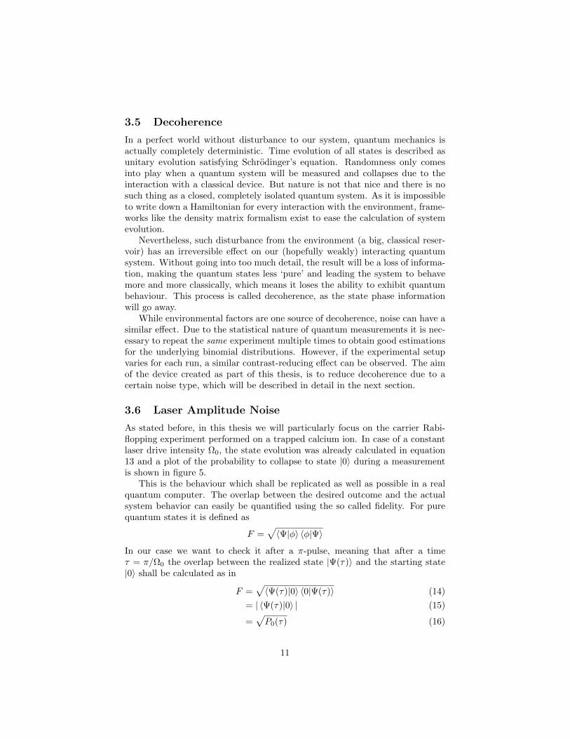
First we want to concentrate on the average gate-intensity offset. In fig.7a this effect is plotted with a simulated acquisition of 500 data points in atimerange of 0 to 6π with a normally distributed laser intensity around Ω0 = 1and 1 % relative standard deviation. For each data point the experiment wasrun 100 times with a data point constant, but randomly chosen laser intensity.Obviously, for later data points such intensity instabilities have a much biggereffect, as the noise will be ‘amplified’ by the pulse duration. A more drasticexample has been computed in figure 7b with a noisier laser. It is obvious thatin such a case the data becomes useless pretty quickly.

The second case we discussed so far was considering faster intensity noisewhich happens in between the acquisition of shots for a single data point. Suchnoise leads to decoherence and a simulation can be found in figure 8 with differ-ent noise levels. Both graphs were calculated using 5000 shots per data point toremove effects on the Rabi frequency when only considering a discrete spectrum.If only a few shots are acquired this will lead to a small frequency shift. Theresults show the predicted behaviour, as more noise leads to a faster decay.

4.3 Post-Selection

To show contrast improvements arising from intensity based data post-selection,carrier flops were recorded in an unstable lab condition with additional intensitynoise introduced on the tapered amplifier as described earlier. The original,complete dataset is plotted in figure 9, where a fast decoherence is obvious. Inthe next step, a histogram of all measured laser intensities is created, such thata small intensity range which includes many data points can be selected. Theresult is shown in figure 10. This particular distribution is vastly different froma gaussian distribution due to its non-natural source and it has been introducedusing a triangular ramp on the tapered amplifier (TA). In theory this shouldresult in an almost rectangular intensity spectrum which then has been distorteddue to non-linearity and hysteresis effects on the TA.

From the histogram it can be seen that a fair amount of data can be extractedby restricting the allowed intensity to values between 57 and 62. This willreduce the relative deviation to approximately 2.5 %. Of course such selectionwill inevitably make statistics worse, as the number of experiments reduces(drastically, under such extreme conditions). But as the confidence only scalesas ≈ 1/

√n (n is the number of experiments per data point), this degradation is

tolerable.Post-selection results based on the parameters written above are displayed

in figure 11. With such a broad original intensity distribution the contrast im-provements are quite remarkable and significant. In the second graph (fig. 11b)the post selected data has been reordered using the measured pulse area instead

15

0 5 10 15 20intended pulse duration (a.u.)

0.0

0.2

0.4

0.6

0.8

1.0

mea

sure

d po

pula

tion

in s

tate

0

(a) Normally distributed intensity noise around Ω0 = 1 with σ = 1 %

0 5 10 15 20intended pulse duration (a.u.)

0.0

0.2

0.4

0.6

0.8

1.0

mea

sure

d po

pula

tion

in s

tate

0

(b) Normally distributed intensity noise around Ω0 = 1 with σ = 5 %

Figure 7: Simulated carrier flopping distortion with normally distributed inten-sity noise that stays constant during a single data point acquisition cycle. Eachplot was simulated with 500 data points and 100 shots per data point. The redline displays an ideal behaviour.

16

0 5 10 15 20intended pulse duration (a.u.)

0.0

0.2

0.4

0.6

0.8

1.0

mea

sure

d po

pula

tion

in s

tate

0

(a) Normally distributed intensity noise around Ω0 = 1 with σ = 1 %

0 5 10 15 20intended pulse duration (a.u.)

0.0

0.2

0.4

0.6

0.8

1.0

mea

sure

d po

pula

tion

in s

tate

0

(b) Normally distributed intensity noise around Ω0 = 1 with σ = 5 %

Figure 8: Simulated carrier flopping decoherence with gaussian distributed in-tensity noise without any correlation to the current data point taken. Each plotwas simulated with 500 data points and 5000 shots per data point to minimizenumerical effects. The red line displays an ideal behaviour.

17

of the intended pulse duration. With this specific set of data results are notparticularly compelling, but it can clearly be seen that it reduces the uncer-tainty on the x-axis. However, it should be noted that these results can varya lot when analyzing different sets of data or even with the chosen data pointdownsampling. With some test runs pulse area reordering showed remarkableimprovements, but it will probably be of more use with much bigger data setswhere the resulting graph contains lots of closely spaced data points and alsomore shots per data point.

4.4 Conclusion

The experimental results have shown that postselection and data reordering canbe used to significantly increase the carrier flopping contrast. Although only asingle dataset is shown, similar results were obtained consistently during soft-ware development test runs. But unfortunately, due to time constraints andgeneral lab equipment state it was not possible to take more sensible measure-ments, e.g. on different gate types or to better understand the electronicallyinduced noise. Comparisons with the measured background intensity show, thatall these results are above of the electronic noise level, but the signal-to-noiseratio could have been better. Many intensity measurements returned values inthe lower 2 % of the analog conversion range, where electronical pickup noiseimmunity would certainly improve if the signal on the photodiodes could beamplified.

Also the preparations and building of the device took a major part of theavailable time for this project. As a result the data acquisition and analysis,as well as statistical evalution are carried out on a very basic level of accuracyand a more detailed study would be helpful. Unfortunately, by the time thedevice was ready to use the general lab setup was in a very unstable state dueto several major changes to the equipment. While this was partly helpful tocheck the validity of this post-selection approach, it also introduced many othernoise sources which are resulting in faster decoherence, even with a very welldefined laser intensity.

5 Experimental Setup

Controlling trapped ions is a delicate task, as good control of many involvedlasers and other devices is needed. For all the processes like readout, cool-ing, repumping, state preparation, gate operations or ionization, wavelengthsof 375 nm, 397 nm, 423 nm, 729 nm, 854 nm and 866 nm are needed in varyingpolarizations and at different times. Moreover, the intensities and especiallyfrequencies have to be very well defined to match the resonance of the corre-sponding transition. Due to all of these requirements, like switching beams onand off electronically or to introduce small detunings to the frequency, manyAOMs (acousto optic modulators) have been put into the beam paths to allowcontrol. Of course they again require driving amplifiers and (digitally controlled)

18

0 20 40 60 80 100pulse time (µs)

0.0

0.2

0.4

0.6

0.8

1.0

estim

ated

pop

ulat

ion

in s

tate

1

(a) The error bars indicate the binomial probability estimation error(95 % confidence) and have been calculated using the Wilson score formula.

0 20 40 60 80 100 120pulse time (µs)

0.0

0.2

0.4

0.6

0.8

1.0

estim

ated

pop

ulat

ion

in s

tate

1

(b) The horizontal error bars correspond to assumed 10 % laser intensity noiseand are calculated using equation 22.

Figure 9: Complete acquired carrier flopping data consisting of a total of 5000equally spaced data points of pulse lengths between 5 and 100 µs. Each datapoint was taken twice and then recombined to show 75 data points as in thegiven plots. 19

50 60 70 80 90 100729nm laser intensity (a.u.)

0

50

100

150

200

250

300

Figure 10: Histogram of the 729 nm laser intensity measured over 10 minuteswith a triangular ramp on the tapered amplifier feedback amplifier resulting inlarge variations for demonstration purposes. Only shots with laser intensitiesbetween 57 and 62 were used for post-selection.

20

0 20 40 60 80pulse length (µs)

0.0

0.2

0.4

0.6

0.8

1.0

estim

ated

pop

ulat

ion

in s

tate

1

(a) Postselected carrier flopping of the same data as in figure 9

100000 200000 300000 400000 500000 600000 700000pulse length (µs)

0.0

0.2

0.4

0.6

0.8

1.0

estim

ated

pop

ulat

ion

in s

tate

1

(b) Postselected and pulse-area sorted Rabiflopping of the same data as infigure 9

Figure 11: Post-selected carrier flopping with individual experiments sorted ac-cording to different parameters. The vertical error bars indicate the binomialprobability estimation error (95 % confidence) and have been calculated usingthe Wilson score formula. Horizontal errors show standard deviations of the ac-tual measured pulse area of all shots which have been assigned to the individualdata point.

21

ZedboardIonizer

RedPitaya

Optional Part. Does not need to be turned on.

reptoarClient

DDS

DDS

...

DEATH 1 DEATH 2

TTL lines

PMTs

Photodiodes

RF

sou

rce Arbitrary waveform players

-> to trap electrodes

Slow, long-termlab equipment

monitoring

Time seriesdatabase server

Acquisition triggerD

EA

TH

tri

gg

er

Figure 12: Schematic overview of the most important electronics involved inexperimental control and data acquisition. Thick blue lines represent ethernetconnections and dotted ones correspond to single line analog (red) or digital(black) inputs/outputs. A high dot frequency will indicate RF capable lines.

RF sources with good timing control.A typical experimental sequence consists of 5 different sections. Starting

with a precooling stage, some near resonant doppler cooling will be appliedbefore preparing the ion in its ground state. Then, the actual gate can beperformed (usually including some 729 nm pulses) and is followed by a readoutphase which determines the state using fluorescence detection. Further detailson this can be found in section 4.3 of [Kie15].

5.1 Lab Computer Control Overview

Such a complex sequence as the one given in the previous section requires goodand reliable triggering of the correct devices at well defined times with smalljitter. Additionally all this has to be synced with other readout devices whichrely on fast acquisition (like photo-multiplier-tubes) and displayed or saved ina user friendly way.

To accomplish all of this, a control architecture has been developed whichcontains several different layers of software and hardware, completing differenttriggering and programming tasks at the required realtime constraints. An

22

overview of everything control related is given in figure 12, which will now bedescribed.

DEATH These devices are not of great importance for the experiments coveredin this thesis. They contain multi channel, high speed digital-to-analogconverters (DACs), which are connected to the individual segmented trapelectrodes and thus provide axial confinement and transport capabilities.Waveforms are programmed using Ionizer and other software tools andthen sent to the internal memory over an Ethernet connection. After-wards, these waveforms can be triggered for playback via a single edge-triggered digital line (usually called TTL in this thesis).

DDS A short term for ‘direct digital synthesis’. They contain sensitive circuitryto synthesize RF signals with a given phase, amplitude and frequency, andare mainly used as digitally controlled signal sources for AOMs. In thecontrol rack these boards with 4-channels each, sit next to the Zedboardand are connected using a backplane board-to-board interconnect.

Zedboard The most important real-time component of the architecture. Itcontains a Xilinx Zynq chip, which is built of a dual-core ARM CPU andan FPGA. The programmable logic contains cores for communicating withand triggering the DDSes, as well as modules to trigger TTLs at specifiedtimes. Both elements are being controlled using FIFO execution queueswhich will be preprogrammed using some experiment-specific code thatruns on the processor. Code is actually executed without an intermediateoperating system layer, but Xilinx library functions are used to handle forexample network communication.

In general, the Zedboard receives settings (like AOM frequencies, pulselengths, ...) from Ionizer and is then responsible for executing a completeexperimental sequence with a single set of parameters n times, and sendingback the PMT readout results afterwards.

Ionizer This software is the visible user interface to run trap experiments. Itis connected to the Zedboard via Ethernet to send the selected experi-ment including parameters. After completion it receives, stores and plotsreturned results. The GUI is able to schedule the execution of multiple,simultaneously selected experiments using a priority system. Since theZedboard only executes a single set of parameters multiple times, Ionizerhandles 1-D and 2-D scans by sending new sets of parameters as soon asneeded, if for example the 729 nm laser pulse duration shall be swept overa certain range. All returned PMT counts from the experimental readoutphase are then individually saved for later data analysis.

Redpitaya New addition to the control system which has been developed inthis thesis and adds post-selection functionality. Its capabilities, function-ality and integration will be extensively covered in the following sections.

23

5.2 RedPitaya Capabilities

The builtin components of a RedPitaya board are quickly explained. It consistsbasically of an almost identical Xilinx Zynq chip as the Zedboard. However,while the hard CPU cores and clock speeds are the same, the programmablelogic part is a bit smaller. This SoC is then complemented with 512MB of DDR3memory, a Gigabit Ethernet port and, the most important part for postselection:Two high speed (125 Msps) analog input channels, as well as two high speedanalog outputs (not needed for this project). Additionally, certain functionalityof the Zynq chip is exposed via pin headers. This includes the ability to slowlyread up to 16 digital inputs, as well as four 12-bit analog inputs up to speeds ofa few Hz.

The Hardware package is provided with an open-source ecosystem, includingsome preprogrammed FPGA bitstream to expose an oscilloscope like function-ality to the CPU, as well as an easily runnable operating system with webapplications to access the high-speed ADC data using a nice graphical userinterface.

As the device is still fairly new and the manufacturer is pushing updates to adevelopment branch almost on a daily basis, one big aim during the developmentin our group was not to touch the hardware part, so that we can easily profitfrom new developments on this side. This actually paid off a few times, as somecritical bugs were fixed in the meantime, and the required DMA feature (seesection 5.4) was added after a while. On the other hand it also complicatedsome things and causes significant slowdown, as missing features have to becompensated with software, which might add delays. Anyhow, especially forprototyping new features the software solution still turned out to be superior,as synthesizing the FPGA bitstream took approximately 15 minutes on a fairlywell equipped workstation.

5.3 Software / Communication Architecture

The Redpitaya’s fast analog input channels are used to capture laser intensitiesduring a single experimental sequence, by measuring voltages of photodiodeswhich are placed in the beam after it passed through the trap. The resultingwaveforms can then be sent to a computer running the ‘reptoar’ Python-basedclient software for further processing and saving. As the two 125 Msps 14-bitADC channels could in theory create up to 3.5 GBit/s of data, sending all thisover a single GBit network adapter seems to be impossible and a bad choice.And indeed, this architecture reduces the rate at which experiments may berun.

On the other hand, there are good reasons to move the data processing tohigher abstraction levels in early stages of development or in a research environ-ment. In both situations requirements and algorithms will change frequentlyand may also be written by persons who don’t want to invest lots of timein learning hardware description languages (HDL) or embedded programming.Additionally, more complex signal processing algorithms might be impossible

24

Ionizer

Zedboard

reptoar client

RedPitaya (buster)

Time

Experim

ent type,

# sho

ts and d

atapo

intssam

ple rate &

count

AC

K

AC

K

Exp

erim

ent

typ

e,d

atap

oin

t p

aram

eter

s results (PM

T counts)

results (PM

T counts)Ex

per

imen

t ty

pe,

dat

apo

int

par

amet

ers

Exp

erim

ent

typ

e,d

atap

oin

t p

aram

eter

s

cap

ture

d w

avef

orm

s

cap

ture

d w

avef

orm

s

Figure 13: Communication timing diagram when the RedPitaya Post-selectionfunctionality is activated and used. Arrows indicate exchanged messages.

25

to convert into HDL or will take much computation time on a processor. Thelatter thing should not happen on the RP’s application processor as it needs tostay responsive for ADC acquisition reprogramming.

To transmit data over the network without adding lots of programming over-head, the ZeroMQ library is being used in combination with msgpack for dataserialization. Especially ZeroMQ adds some network and processing overheadand therefore reduced the achievable throughput to ≈ 300 MBit/s. But usingthis widely adopted and well maintained library reduces our custom code com-plexity by a fair amount and therefore has a good impact on maintainabilityand stability.

A timing diagram of the RP communication is shown in fig. 13. Between’reptoar-buster’ and the reptoar client multiple message channels are open, allwith a distinct purpose:

RPC This remote procedure call interface follows a strict request-response pat-tern, which is used to send commands from the reptoar-client to the RP.Such commands may lead to reconfiguring of ADC sample rates and du-rations, or a start/stop of streaming operation.

Streaming Used to send waveforms to interested clients in realtime. Uses theZeroMQ publisher-subscriber pattern and is configured to quickly droppackages such that latencies are short.

Capture Sends the same type of packages as the streaming channel, but inpush-pull configuration. This way it can be ensured that no message(waveform data) will be lost if the receiver can’t keep up with the datarate for a short amount of time.

While the RPC channel is always open to receive commands, the streaming andcapturing channel will be used depending on the currently selected experimentand mode. For post-selection, with a known amount of data points the capturechannel is active, while for continuously running experiments the streamingchannel will be used to give an oscilloscope like, realtime waveform display.The purpose of the reptoar client is to read Ionizer’s synchronization messagewhich contains the next experiment type and total expected amount of shots.This information will be connected with a configuration file to determine therequired sampling settings. These are then sent to the Redpitaya. As soon asthis is completed and the RP is ready for acquisition, Ionizer will be notifiedsuch that it can contact the Zedboard to start the experimental sequence.

For every incoming trigger, the reptoar-buster tool running on the RP willsend captured waveforms out over the selected streaming or capturing connec-tion. Usually these are received by the client, which then selectes the post-processing methods based on the configuration file and currently running ex-periments. In case of a capturing operation, as soon as the expected amount oftriggers has been received the resulting, post-processed data will be saved to a.csv file for later analysis in combination with Ionizer’s shot log.

Finally, a few words on the choice of Arch Linux as operating system. Afterwe used the prepackaged ‘Redpitaya OS’ distribution for a while, it turned out

26

that it is not very suitable for native application development. It does not comewith a compiler installed, and cross-compiling applications on the developmentcomputer (as well as the required libraries) is possible at best, but usually verycomplicated. Trying to remotely debug our custom data acquisition tools thenfinally motivated a change to a new distribution as version mismatches betweenthe host and target made it a nightmare to hunt down bugs.

5.4 Datapath / High-Speed Acquisition

As written in the previous section, both ADCs are able to produce big amountsof data very quickly. In order to make sure that no sample is being lost, usuallythe data will be pushed to a 16384 sample sized Block-RAM ring buffer withinthe FPGA. In the original configuration this buffer is then memory mappedand accessed using the general purpose 32-bit wide AXI (Advanced eXtensibleInterface) bus interface between the processing system and programmable logic.However, as it turned out this particular bus interface bandwidth is way toosmall, as data rates cut at approximately 2 Mbit/s.

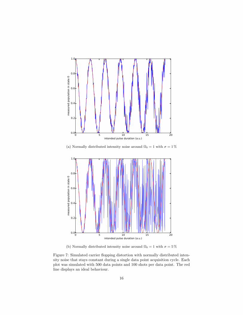
Figure 14 shows the new, direct-memory-access (DMA) based solution. Herethe operating system reserves contiguous memory regions in the DDR3 sys-tem memory, which are then accessed directly from the FPGA using a high-performance 64-bit AXI bus interface. In the current configuration the CPUwill then poll status registers on a regular basis for acquisition completion andmake a memory copy as soon the scope module is done writing. After thismemory copy operation the reserved DMA memory can again be used to storethe next waveform. This process is a lot quicker than the old one, as opti-mized MDSI (multiple data, single instruction) commands provide a lot morebandwidth on the system memory than on the general purpose AXI bus.

Nevertheless, DMA based solutions are tricky to program, and the used ap-proach gives some improvement, while still leaving room for many optimizationswhich will allow even smaller trigger dead times. More on this in section 6. As aproof of concept, the current implementation contains a small and simple kernelmodule which allocates the required contiguous physical memory regions on loadtime and writes the corresponding lower- and upper boundary addresses to thecorrect configuration registers of the AXI DMA controller module. This modulealso offers status registers (current and trigger write addresses) which can beused with a polling algorithm to check if the acquisition has been triggered andis completed.

So all in all, the job of the ‘reptoar-buster’ tool, which runs on the RedPitayaitself, is to read scope configurations received from the client, write them to theircorresponding registers, wait for triggers, copy the data from the DMA region toa ZeroMQ message and send them back over the correct streaming or capturingchannel.

27

Central Interconnect Bus

APUCache/

MemoryController

Zynq-7010 AP SoC

Ethernet

SCOPEmodule

AXI DMAcontroller

FPGABRAM

SampleBuffer

ADC

DD

R3

Sys

tem

Mem

ory

Processing System (PS)

Programmable Logic (PL)

Figure 14: Connection diagram of the different soft- and hard-core modulesinvolved in data acquisition on the RedPitaya. Arrows always point from themaster device to the connected slave. Red indicates the slow general purposeAXI bus, while blue arrows are part of the new, DMA-based data path.

28

5.5 Postprocessing

Due to various reasons which were described in section 5.3, post-processing ofthe acquired waveforms is done on a full-blown workstation running the reptoar-client Python program. This keeps track of the currently running experimentand then uses a configuration file to pass received waveforms to the correctand helpful processing units (PU). In the client two different base types of PUsare available. The first one, a WaveformProcessor may add a completely newwaveform to the raw ones received from the RedPitaya. Typical use cases arefor example calculations of a moving average or background subtraction. Thesecond type, a DatapointProcessor will calculate usually a small, finite amountof new data points which have nothing to do with time anymore. As an exampleone can think of an experiment which pulses different lasers on seperately forshort times. Then some kind of algorithm can calculate the mean peak heightfrom each of these pulses to compare individual laser intensities between severalexperiments and over a longer amount of time. Also, in case of the post-selectionexperiment a similar technique was used, where a DatapointProcessor measuresthe mean height of the 729 nm pulse, which is then used to calculate the area.

The client program also includes a simple GUI to display current waveformsand their processed data points as a nice, shot-to-shot timeseries, such that itcan be used as a simple oscilloscope on the attached channels and to monitortime variations of important quantities. While the complete waveforms wouldbe too much data to store over a longer time period, processed data points arealso stored in a time-series database.

5.6 Long-term Logging

The Zynq SoC chip with the shipped RedPitaya hardware configuration allowsfor additional data acquisition using the built-in XADC module, which can beused for slow analog voltage readout of 4 external pins. On top of this, 16 digital(15 usable, as one is used as external trigger input) input pins are accessiblevia readout status registers, to query their state. Reading these values is aslow process, so it is only suitable for DC voltages (2 Hz readout rate), butsuch functionality is very helpful to monitor laboratory equipment over longerperiods of time. The currently installed configuration for example monitorsvoltages applied to cavity piezos or thermocouples to get a better overview ofcorrelations which affect laser system stabilities.

The digital channels, on the other hand, can be used to log or display statusof systems like the Calcium ovens, PID lock states, and other events which canbe thresholded or converted into a digital signal. But one has to be aware thatthese inputs are also only polled on a large time interval basis, so short eventsmight be missed. The solution for this problem will be discussed in the nextsection.

To actually store and display all this logging data, a ready-to-use open sourcetime series database called InfluxDB is being used. For this also nice and eas-ily configurable web interfaces for realtime display and historic browsing are

29

Figure 15: 3D breakout board assembly visualization.

available. Our choice fell to Grafana, which provides excellent support for thisspecific database. Both these services run on an always-on database serverthat also has been indicated in figure 12. Additionally, it hosts a small scriptwhich receives logging broadcasts and converts them into the correct databaseAPI format. These broadcasts are emitted via small daemons (‘reptoar-logger’)running on the RedPitayas and sending out the logging messages in a publisher-subscriber ZeroMQ pattern.

5.7 Breakout Board

Figure 16: Digital pulseextension and overvolt-age protection circuitry

As all the slow, long-term logging inputs are ex-posed via pin headers, it is very hard to make re-liable and easy-to-use connections in a crowded labenvironment. On top of this, the described event-miss possibility for short pulses on the digital chan-nels renders them useless for many applications thatonly emit brief pulses. An example for such appli-cation is a mains glitch/spike detection box built byFrieder Lindenfelser, which generates short pulsesof unknown height if there are disturbances on theelectric supply network. The unknown and possi-ble high output voltage height also imposes a threatwhen connected directly to the FPGA, as high volt-age can destroy circuitry without protection.

To eliminate all these shortcomings a breakoutboard has been designed which will connect to theRP’s pin headers and make them easily accessiblevia SMA connectors, a cable type very commonlyused in our lab. Furthermore, some circuitry wasdesigned to improve the useability of the digital in-puts with respect to the following design goals:

30

• Selectable 50 Ω termination

• Overvoltage protection

• Pulse extension circuitry

The latter should make sure that short, digital pulses are extended to a durationwhich cannot be missed by the 2 Hz polling interval. Therefore a so calledmonostable multivibrator IC is used, which triggers a configurable length outputpulse on a positive edge at the input pin. The circuit is shown in figure 16. Ata first stage, the dip switch allows to configure the connection to a 500 mWtermination resistor which can be used for input voltages up to 5 V. A seconddip switch can be used to select a possible input signal inversion using a XORgate, as the multivibrator expects a positive edge signal. This output is then sentto the pulse extender and recombined using an OR gate with the multivibratoroutput. This results in a final signal being sent to the FPGA which is high aslong as the input signal is being pulsed, but at least 1 second long.

6 Conclusion and Outlook

This project has been developped as a proof of concept for the usefulness ofdata post-selection in quantum information experiments. Additionally it hasproven to be very useful as a lab equipment status monitoring device of bothslow moving analog and digital channels, as well as realtime experimental con-ditions. The resulting post-selected data sets showed significant improvementswith respect to longer coherence times. The visibility of this effect was evenmore surprising as all of this data was taken in an unstable laboratory environ-ment and post-selection reduced an already small dataset to a really tiny one.On the other hand, results of individual shot reordering based on the measuredpulse area were promising in theory, but the acquired data could not keep upwith high expectations. The reasons for this are unknown, but probably ourassumptions were too strict compared to the real-world experimental setup.

In addition to this experimental part a theoretical calculation of decoherenceeffects due to intensity noise has been carried out, resulting in useful formulas toestimate required stability and possible effects in future setups. While currently,in stable lab condition timeframes, the intensity noise does not seem to be amajor source of decoherence, the proposed scheme of post-selection can be ofgood use as soon as more complex single- and multi-qubit gates are consideredwhich will include longer pulse durations.

As with any prototyping project, further possibilities for improvement weredeveloped over the meantime. First, the fast acquisition DMA part would ben-efit a lot of increased sample buffer sizes and DMA pooling, a technique whichassigns a new and empty memory region immediately after the previous writeis done. This way the old data can be copied and transmitted while the nextshot is already being acquired. This would help to get rid of the wait-time com-pletely, which currently can’t be used as the RP has to first send and empty the

31

buffer before new data may be written into it. Also algorithms may be com-pletely moved into the hardware as soon as they have become stable and provento be effective. At least for thresholding or the calculation of means this coulddrastically improve post-processing computation times. Another very helpfuladdition would include a digitally implemented, configurable delay of the ana-log input channels. This would allow to record gate operations and the followingreadout phase at the same time which could be used to detect a dark ion dueto a briefly unlocked 397 nm laser.

Regarding the long-term logging abilities of the RedPitaya also various im-provements are possible. A major thing which did not make it onto the firstprototype breakout board is the missing voltage clamping at the trigger line.Also the amount of slow analog input channels is small, as they quickly becamevery successful in the lab. Multiple solutions are possible to overcome this prob-lem. Multiplexing would be one, but it might also be interesting to get moreaccurate and precise measurements. An additional ADC for this could easilybe added as an SPI or I2C bus interface is also exposed. Such steps towards aglobal lab monitoring system seem to be very welcome and might become aninteresting project for a future student.

32

References

[Fey82] RichardP. Feynman. “Simulating physics with computers”. English.In: International Journal of Theoretical Physics 21.6-7 (1982), pp. 467–488. issn: 0020-7748. doi: 10.1007/BF02650179. url: http://dx.doi.org/10.1007/BF02650179.

[Deu85] D. Deutsch. “Quantum Theory, the Church-Turing Principle and theUniversal Quantum Computer”. In: Proceedings of the Royal Soci-ety of London A: Mathematical, Physical and Engineering Sciences400.1818 (1985), pp. 97–117. issn: 0080-4630. doi: 10.1098/rspa.1985.0070.

[Sho94] P. W. Shor. “Algorithms for Quantum Computation: Discrete Log-arithms and Factoring”. In: Proceedings of the 35th Annual Sympo-sium on Foundations of Computer Science. SFCS ’94. Washington,DC, USA: IEEE Computer Society, 1994, pp. 124–134. isbn: 0-8186-6580-7. doi: 10.1109/SFCS.1994.365700. url: http://dx.doi.org/10.1109/SFCS.1994.365700.

[Sho95] Peter W. Shor. “Scheme for reducing decoherence in quantum com-puter memory”. In: Phys. Rev. A 52 (4 Oct. 1995), R2493–R2496.doi: 10.1103/PhysRevA.52.R2493. url: http://link.aps.org/doi/10.1103/PhysRevA.52.R2493.

[Ste96] Andrew Steane. “Multiple-Particle Interference and Quantum Er-ror Correction”. In: Proceedings of the Royal Society of London A:Mathematical, Physical and Engineering Sciences 452.1954 (1996),pp. 2551–2577. issn: 1364-5021. doi: 10.1098/rspa.1996.0136.

[DiV00] David P. DiVincenzo. “The Physical Implementation of QuantumComputation”. In: Fortschritte der Physik 48.9-11 (2000), pp. 771–783. issn: 1521-3978. doi: 10.1002/1521- 3978(200009)48:9/

11<771::AID-PROP771>3.0.CO;2-E. url: http://dx.doi.org/10.1002/1521-3978(200009)48:9/11%3C771::AID-PROP771%3E3.

0.CO;2-E.

[NC00] Michael A. Nielsen and Isaac L. Chuang. Quantum Computation andQuantum Information. Cambridge University Press, 2000.

[HRB08] H. Haffner, C.F. Roos, and R. Blatt. “Quantum computing withtrapped ions”. In: Physics Reports 469.4 (2008), pp. 155–203. issn:0370-1573. doi: http://dx.doi.org/10.1016/j.physrep.2008.09.003. url: http://www.sciencedirect.com/science/article/pii/S0370157308003463.

[Har13] Thomas P. Harty. “High-Fidelity Microwave-Driven Quantum Logicin Intermediate-Field 43Ca+”. PhD thesis. 2013.

33

[JNN13] J.R. Johansson, P.D. Nation, and Franco Nori. “QuTiP 2: A Pythonframework for the dynamics of open quantum systems”. In: ComputerPhysics Communications 184.4 (2013), pp. 1234–1240. issn: 0010-4655. doi: http://dx.doi.org/10.1016/j.cpc.2012.11.019.url: http://www.sciencedirect.com/science/article/pii/S0010465512003955.

[Kie15] Daniel Kienzler. “Quantum Harmonic Oscillator State Synthesis byReservoir Engineering”. PhD thesis. 2015.

[Ame+] Ben Ames et al. Nanofiber. url: http://www.quantumoptics.at/index.php/en/research/nanofiber (visited on 06/29/2015).

[Glo] Glosser.ca. Bloch Sphere. url: https://commons.wikimedia.org/wiki/File:Bloch_Sphere.svg (visited on 06/29/2015).

[Mos] Mostafa. Quadrupole Potential Generation in Paul traps. url: http://physics.stackexchange.com/questions/82291/quadrupole-

potential-generation-in-paul-traps (visited on 06/29/2015).

34