IMPROVING MICROSCALE CALORIMETRY USING FULL FIELD DATA

CAPTURE OF NANOHOLE ARRAY TRANSMITTANCE MEASUREMENTS

A Thesis Presented

By

Timothy Edwin Beck Sanborn

to

The Department of Mechanical and Industrial Engineering

in partial fulfillment of the requirements

for the degree of

Master of Science

in the field of

Mechanical Engineering

Northeastern University

Boston, Massachusetts

December 2017

i

ACKNOWLEDGEMENTS

First for foremost, I would like to thank Professor Gregory Kowalski. You have

been a great mentor to me since my undergraduate years at Northeastern University. As a

graduate, you allowed me to join you in your research and I am forever grateful to you for

that. This has been a great learning experience for me am I’m sure the lessons will not be

forgotten soon.

I would like to thank Masoud Modaresifar, who’s knowledge and guidance has

been a catalyst for me on many occasions. Your willingness to assist me whenever I needed

was very kind, and I am very appreciative.

I would like to thank my parents, Tim and Emily. You have given me so much to

be appreciative of in my life, and I remind myself of that every day. You have helped me

through every step of this arduous process and I love you very much.

I would also like to thank my brother, Michael. I have always tried to pursue

excellence in the things I do so that I may set a good example for you. You have helped

me in far more ways than you know. I love you.

Lastly, I would like to thank everyone else in my life who has helped me during my

education. There are many people who have pushed me to improve myself throughout my

life, and it has made me a better person.

I will always remain a student of life.

ii

TABLE OF CONTENTS

List of Figures ........................................................................................................ iv

Abstract ................................................................................................................ viii

1 Introduction ...................................................................................................... 1

2 Background ....................................................................................................... 2

2.1 Calorimetry................................................................................................ 2

2.1.1 Differential Scanning Calorimetry ...................................................... 6

2.1.2 Isothermal Titration Calorimetry ........................................................ 9

2.2 Surface Plasmon Resonance and Extraordinary Optical Transmission .. 10

2.3 Current Approach/Previous Work ........................................................... 15

2.3.1 Experimental Setup ........................................................................... 15

2.3.2 Sensor Location Method ................................................................... 21

2.3.3 Previous DSC Work .......................................................................... 24

3 Approach and Methods ................................................................................... 25

3.1 Field Capture Programs ........................................................................... 26

3.1.1 Basic Capture Program...................................................................... 26

3.1.2 Region-of-Interest Control Edition ................................................... 28

3.1.3 Temperature Control Edition ............................................................ 30

3.2 Postprocessing Programs......................................................................... 33

3.2.1 Method/Development ........................................................................ 33

3.2.2 Debugging ......................................................................................... 35

iii

3.2.3 Multiple Sensor Analysis .................................................................. 40

3.2.4 Single Sensor Analysis ...................................................................... 41

4 Tests and Results ............................................................................................ 42

4.1 Comparison to Sensor Location Method ................................................. 42

4.1.1 General Procedure for Comparison Injection Test ............................ 43

4.1.2 Results and Discussion ...................................................................... 44

4.2 Sensor Tracking....................................................................................... 47

4.3 Capture Speed Tests ................................................................................ 48

4.4 Effect of Number of Averaged Sensors on Overall EOT ........................ 51

4.5 Effect of NHA Chip Surroundings on EOT Experiments ....................... 54

4.5.1 Procedure ........................................................................................... 55

4.5.2 Experimental Setup ........................................................................... 56

4.5.3 MATLAB Simulation ....................................................................... 58

4.5.4 Results ............................................................................................... 59

4.6 Fringe Identification ................................................................................ 63

5 Conclusions .................................................................................................... 67

6 Recommendations and Future Work .............................................................. 68

References ............................................................................................................. 70

Appendix ............................................................................................................... 73

iv

LIST OF FIGURES

Figure 1: Schematic overview of the process for selecting recombinant antibodies

for diagnostic use [8] .......................................................................................................... 3

Figure 2: Thermodynamic signature of all HIV-1 protease inhibitors approved by

the FDA from 1995 to 2006 [1] [2] .................................................................................... 6

Figure 3: Schematic of Differential Scanning Calorimeter [15] ............................. 7

Figure 4: An example DSC trace for the reversible unfolding of a monomeric

protein. The maximum of the heat capacity curve is the Tm and is 60°C. The dashed lines

are the linear extrapolations of the pre- and post-transition baselines into the transition

region. The difference between these values at Tm is the ΔCp. The thick black line is the

theoretical ‘progress’ baseline. [11] .................................................................................... 8

Figure 5: A) Schematic of ITC experimental setup. B) Raw Data captured from ITC

experiment. C) Reported data after analysis to determine Binding constant (Kb),

stoichiometry (n) and enthalpy of reaction (ΔH) [16] ...................................................... 10

Figure 6: Schematic of the setup used by Krishnan et al. and the temperature sensor

proposed by Kowalski et al. [4] ........................................................................................ 12

Figure 7: Experimental zero-order transmission spectra of a Au film on a quartz

substrate (𝜀𝑆 = 2.31), as a function of refractive index 𝜀𝐿. The film thickness is 250 nm,

the hole diameter is 200 nm, and the lattice constant is ao = 600 nm [22] ....................... 13

Figure 8: The relationship of the transmitted light through a nanohole array at 750

nm as a function of the dielectric constant using the data of Krishnan et al. [22] for Au film

on a quartz substrate [4] .................................................................................................... 14

Figure 9: (A) An example NHA chip. Each yellow dot is a sensor with a separation

of L = 30 μm. (B) The diameter of each nanohole is d = 150 nm and the lattice constant is

a0 = 350 nm ....................................................................................................................... 15

Figure 10: Whole chip (NHA not visible in center) ............................................. 16

v

Figure 11: Schematic of the optical test setup with an LED light source [3] ....... 16

Figure 12: Image taken of the laboratory setup at Northeastern University, Boston,

MA .................................................................................................................................... 17

Figure 13: Wavelength Electronics LFI-3751 PID temperature controller .......... 17

Figure 14: Exploded view of the flow cell assembly used in the experimental setup.

From left to right: ABS clamp top, glass cover, PDMS flow cell, NHA chip, copper heat

sink, thermoelectric heater, ABS clamp bottom [3] ......................................................... 18

Figure 15: T-sensor type design of flow cell [3]................................................... 19

Figure 16: Chamber flow cell assembly. Mixing of the two inlets (typically bottom,

solvent, and right, solute) occurs in the circular chamber (middle). The left inlet is for the

thermistor and air flow ...................................................................................................... 20

Figure 17: Schematic of the chamber flow cell used in this study [5] .................. 20

Figure 18: Front panel of the calibration program used to determine the sensor

locations prior to an experiment. Exposure of 50000 saturates the camera. ..................... 22

Figure 19: A screenshot of the current program used in the laboratory to collect

EOT data. The 'Cursors' shown on the left side are the pixel locations of the selected

sensors, which are highlighted by red plus-signs on the right side in the NHA output image

........................................................................................................................................... 23

Figure 20: Comparison of different NxN averaging values to determine which value

produced the most accurate data [25] ............................................................................... 24

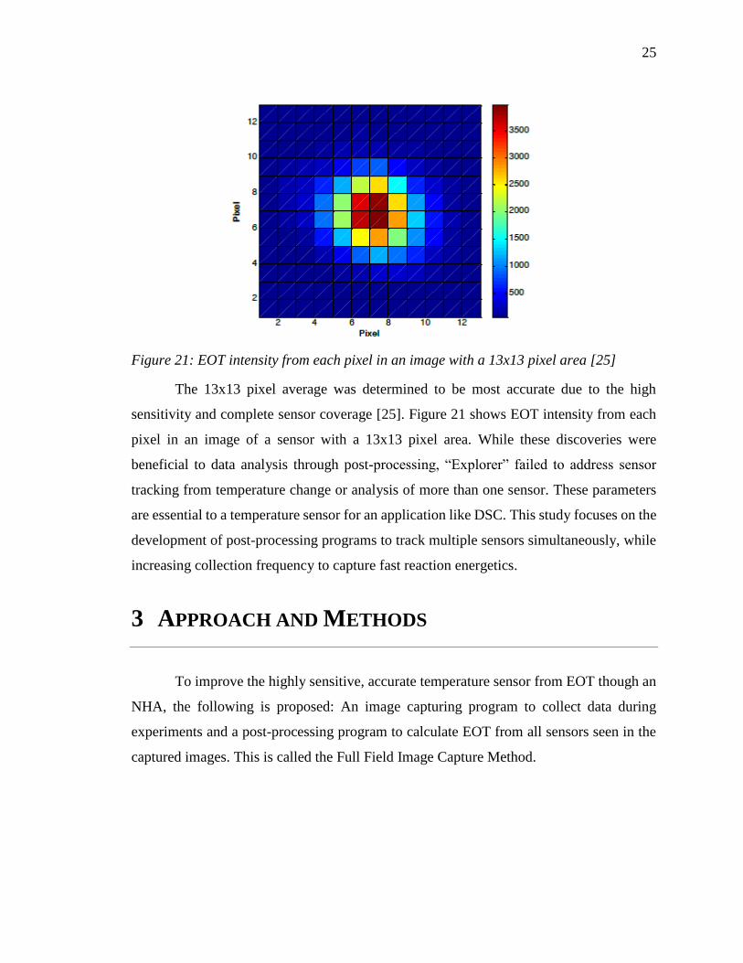
Figure 21: EOT intensity from each pixel in an image with a 13x13 pixel area [25]

........................................................................................................................................... 25

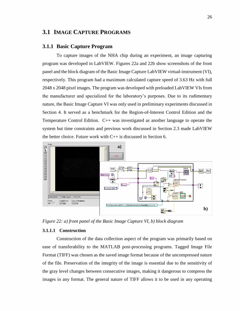
Figure 22: a) front panel of the Basic Image Capture VI, b) block diagram ........ 26

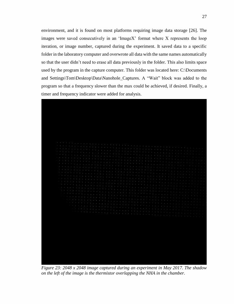
Figure 23: 2048 x 2048 image captured during an experiment in May 2017. The

shadow on the left of the image is the thermistor overlapping the NHA in the chamber. 27

Figure 24: Front panel of the ROI Control Edition VI; in this case, a 100 x 100 pixel

image is shown and captured ............................................................................................ 29

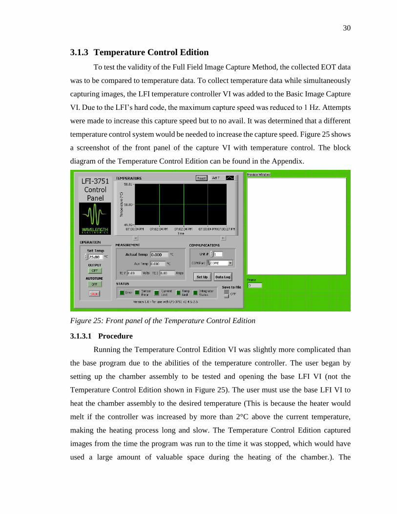
Figure 25: Front panel of the Temperature Control Edition ................................. 30

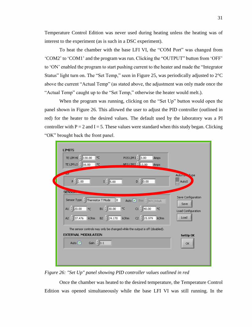
Figure 26: "Set Up" panel showing PID controller values outlined in red ........... 31

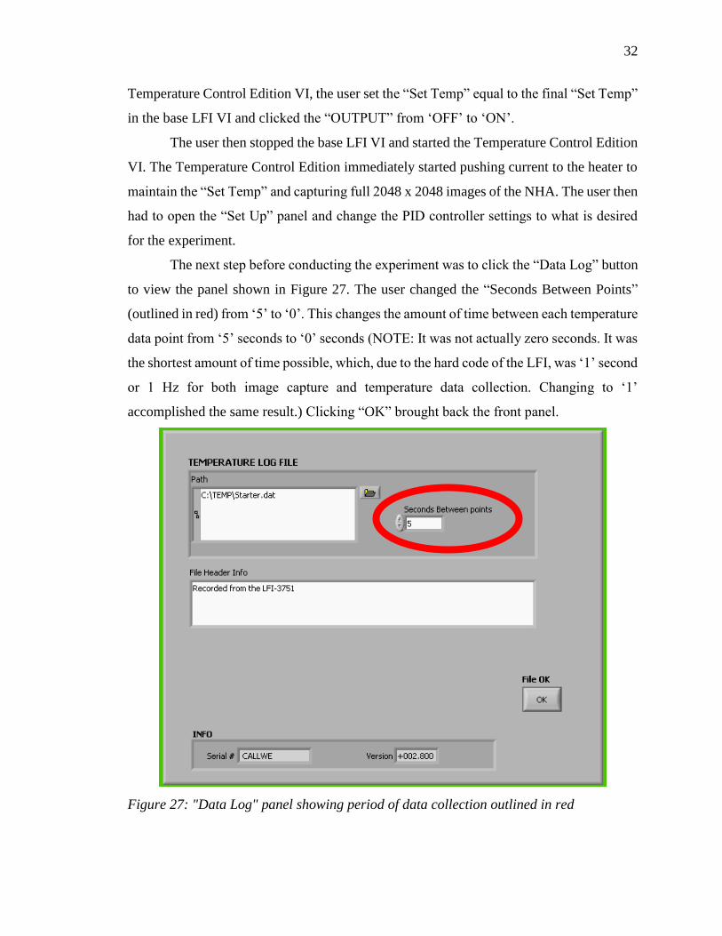
Figure 27: "Data Log" panel showing period of data collection outlined in red .. 32

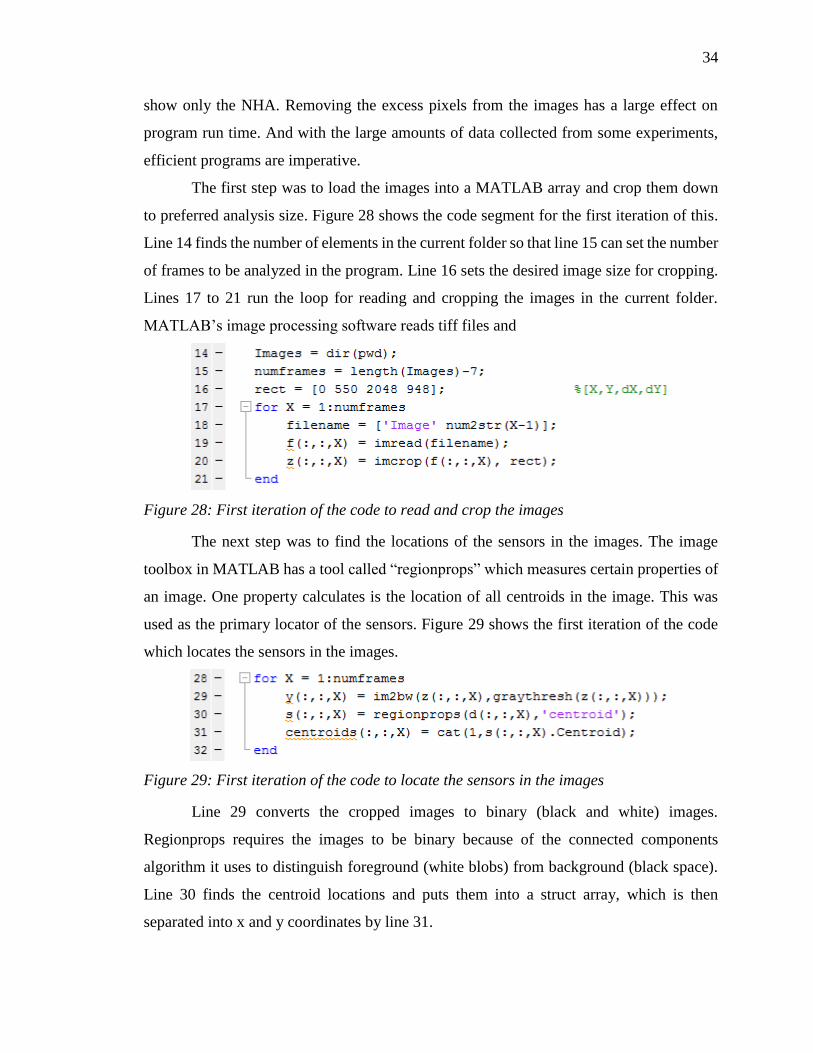
Figure 28: First iteration of the code to read and crop the images ....................... 34

vi

Figure 29: First iteration of the code to locate the sensors in the images ............. 34

Figure 30: First iteration of the code to create the ROI arrays of the sensors ...... 35

Figure 31: First iteration of the code to crop and average each sensor................. 35

Figure 32: The left edge of a captured image showing two partially cut off sensors

........................................................................................................................................... 37

Figure 33: a) Sensor near left edge of image. b) Sensor near right edge of image.

........................................................................................................................................... 38

Figure 34: Chip image displaying the effect of fringes on the light transmission

through the NHA. The darkened areas are the fringes in the fluid. .................................. 39

Figure 35: Locations and Names of Sensors for the two methods in the Comparison

to Sensor Location Method Tests. Sensor Location Method numbers in Blue, Full Field

Image Capture Method numbers in Red. Sensors are arrowed in Green and renamed for

referencing purposes in this study. .................................................................................... 44

Figure 36: Proportional Comparisons of the Sensor Location Method vs. the Full

Field Image Capture Method; a) Top Right; b) Top Left; c) Middle Right; d) Bottom Left;

e) Bottom Right; f) All Sensors Averaged ........................................................................ 46

Figure 37: Pixel Coordinates vs. Time(s). Sensor Travel Path during Air Jet Tests

(see Section 4.4). The red dashed line represents the start time of the air jet. .................. 47

Figure 38: Capture Speed (Hz) vs. Total Number of Pixels ................................. 50

Figure 39: 9 Sensor Average EOT vs. Time for Injection of Ethanol into Water 51

Figure 40: 30 Sensor Average EOT vs. Time for Injection of Ethanol into Water

........................................................................................................................................... 52

Figure 41: 220 Sensor Average EOT vs. Time for Injection of Ethanol into Water

........................................................................................................................................... 52

Figure 42: 422 Sensor Average EOT vs. Time for Injection of Ethanol into Water

........................................................................................................................................... 53

Figure 43: 1341 Sensor Average EOT vs. Time for Injection of Ethanol into Water

........................................................................................................................................... 53

Figure 44: Schematic of Copper setup .................................................................. 56

Figure 45: Schematic of ABS Setup ..................................................................... 57

Figure 46: Schematic of Gap Gold to Light Setup ............................................... 57

vii

Figure 47: Gap Gold to Camera Setup .................................................................. 58

Figure 48: Simulated thermal response of both sides of the NHA chip. L = 0 m

represents the exposed side jetted with air. L = 0.001 m represents the opposite side. .... 59

Figure 49: ΔEOT vs. time (s) for the Single Sensor Air Jet tests with 4 different

configurations. The red dashed lines represent the beginning and end of the air jet. a)

Copper Plate Setup – tjet = 2.0 s, b) ABS Plate Setup – tjet = 2.1 s, c) Gap Gold to Light

Setup – tjet = 2.5 s, d) Gap Gold to Camera Setup – tjet = 2.4 s ......................................... 60

Figure 50: ΔEOT of the Copper Plate Setup vs. Inverse Thermal Response of the

Exposed Face of the NHA chip. The red dashed lines represent the beginning and end of

the air jet. .......................................................................................................................... 62

Figure 51: EOT (CCD Units) vs. Time (s) of an injection test. 30 μL of ethanol into

115 μL of water at 30 μL/min. The red circle highlights a place where suspected fringes

are located due to the sudden change in EOT. .................................................................. 64

Figure 52: Raw data capture during an injection experiment. Fringes are highlighted

moving across the NHA chip in red (1), blue (2), and yellow (3). ................................... 67

Figure 53: Full block diagram for the Temeprature Control Edition VI .............. 73

Figure 54: Multiple_Sensor_Tracking.m code used in post-processing ............... 74

Figure 55: Multiple_Sensor_No_Tracking.m code used in post-processing ........ 75

Figure 56: Single_Sensor_Tracking.m code used in post-processing a single sensor

........................................................................................................................................... 76

Figure 57: Single_Sensor_No_Tracking.m code to post-process a single sensor 76

Figure 58: "Explorer" from Cerroblanco [25] ...................................................... 77

viii

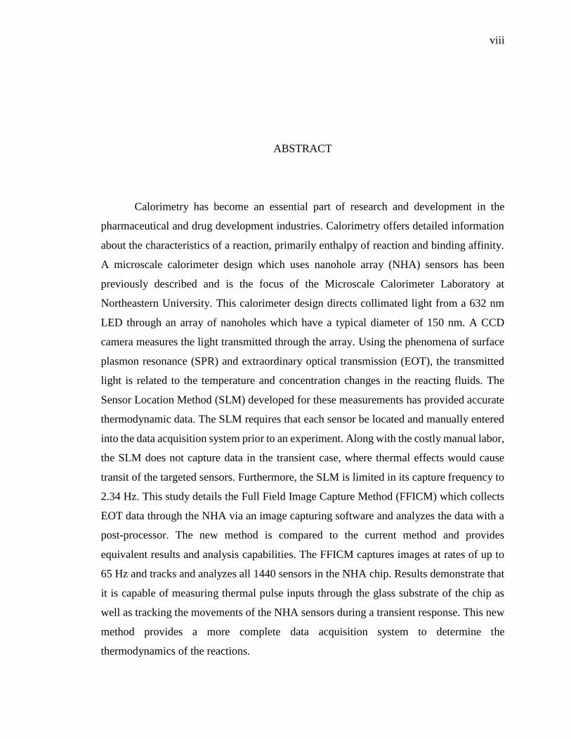
ABSTRACT

Calorimetry has become an essential part of research and development in the

pharmaceutical and drug development industries. Calorimetry offers detailed information

about the characteristics of a reaction, primarily enthalpy of reaction and binding affinity.

A microscale calorimeter design which uses nanohole array (NHA) sensors has been

previously described and is the focus of the Microscale Calorimeter Laboratory at

Northeastern University. This calorimeter design directs collimated light from a 632 nm

LED through an array of nanoholes which have a typical diameter of 150 nm. A CCD

camera measures the light transmitted through the array. Using the phenomena of surface

plasmon resonance (SPR) and extraordinary optical transmission (EOT), the transmitted

light is related to the temperature and concentration changes in the reacting fluids. The

Sensor Location Method (SLM) developed for these measurements has provided accurate

thermodynamic data. The SLM requires that each sensor be located and manually entered

into the data acquisition system prior to an experiment. Along with the costly manual labor,

the SLM does not capture data in the transient case, where thermal effects would cause

transit of the targeted sensors. Furthermore, the SLM is limited in its capture frequency to

2.34 Hz. This study details the Full Field Image Capture Method (FFICM) which collects

EOT data through the NHA via an image capturing software and analyzes the data with a

post-processor. The new method is compared to the current method and provides

equivalent results and analysis capabilities. The FFICM captures images at rates of up to

65 Hz and tracks and analyzes all 1440 sensors in the NHA chip. Results demonstrate that

it is capable of measuring thermal pulse inputs through the glass substrate of the chip as

well as tracking the movements of the NHA sensors during a transient response. This new

method provides a more complete data acquisition system to determine the

thermodynamics of the reactions.

1

1 INTRODUCTION

Lead discovery of candidate drugs is slowed by the limitations of conventional

high-throughput screening (HTS) techniques, eliciting interest in more robust methods of

early stage testing. Current HTS methods, like affinity testing, do not provide enough

information on the binding parameters of the reactions due to the binding affinities between

the candidate compounds being too similar. This presents difficulties when attempting to

decide which compounds to select for further testing, making the data produced by the HTS

method very valuable. Furthermore, current research and instrument development is

focused on extracting information using as little candidate compound mass as possible.

This minimizes the monetary and temporal requirement for each test candidate [1]. The

goal, therefore, is to deduce as much information as possible, as early as possible in the

candidate progression, while minimizing the mass of each tested drug reaction. Calorimetry

is one tool that can achieve this.

Calorimetry has become an essential part of research and development in the

pharmaceutical and drug development industries. Calorimetry offers detailed information

about the characteristics of a reaction; primarily the enthalpy of reaction, ΔH, and the

equilibrium constant, Kc. From these parameters, the entropy of reaction, ΔS, and Gibbs

free energy, ΔG, can be calculated. The enthalpy of reaction describes the amount of energy

used in bonding the reactants. The entropy of reaction describes the amount of energy per

unit temperature unable to be used in the reaction, otherwise known as the irreversibility.

Freire [2] has shown that, for some drug classes, smaller entropy losses and greater

enthalpy contributions have distinguished best-in-class from first-in-class drugs. The two

main calorimetric approaches are Isothermal Titration Calorimetry (ITC) and Differential

Scanning Calorimetry (DSC), discussed in depth in Sections 2.1.1 and 2.1.2.

Current research and development in Calorimetry focuses on minimizing cost by

reducing experiment time and using less compound during testing. Microfluidics has been

a catalyst to produce miniature sensors which achieve these goals [3]. The focus of the

Microfluidics Laboratory at Northeastern University has been the development of a

microscale calorimeter which uses the phenomena of Surface Plasmon Resonance (SPR)

2

and Extraordinary Optical Transmission (EOT) to measure the temperature of a dielectric

[3] [4] [5] [6] [7]. This microscale calorimeter design provides high sensitivity, fast

response, and multiplexed (observing more than one reaction at a time) capabilities. The

Sensor Location Method (SLM) developed for use with the calorimeter has provided

accurate thermodynamic data [5].

The Sensor Location Method requires the targeted sensors to be located and

manually entered into the data acquisition system prior to an experiment. The manual labor

is costly and limited the number of nanohole array (NHA) sensors that can be used in an

experiment. Along with the costly manual labor, the SLM does not capture data in the

transient case, where thermal effects would cause transit of the targeted sensors.

Furthermore, the SLM is limited in its capture frequency to 2.34 Hz. The drawbacks of the

SLM required the development of a new method of data acquisition.

This study details the development of the Full Field Image Capture Method

(FFICM), a new method of data acquisition to be used with the laboratory’s microscale

calorimeter. This method uses an image capturing program to collect data during

experiments and a post-processing program to calculate EOT from all sensors seen in the

captured images.

The results validate that the FFICM produces equivalent results to the SLM. They

also demonstrate that the FFICM is capable of measuring thermal pulse inputs through the

glass substrate of the NHA chip as well as tracking the movements of the NHA sensors

during a transient response.

2 BACKGROUND

2.1 CALORIMETRY

In lead discovery, high-throughput screening (HTS) methods are used to analyze

the interaction between a potential drug candidate (antibody) and a target protein. Current

technology is mostly limited by binary results data (hit/no hit) making it only useful in

initial stage testing [1]. While these techniques can analyze large numbers of candidates

3

quickly, the limited information produced has elicited interest in more robust techniques

that provide more data on each reaction earlier in the process.

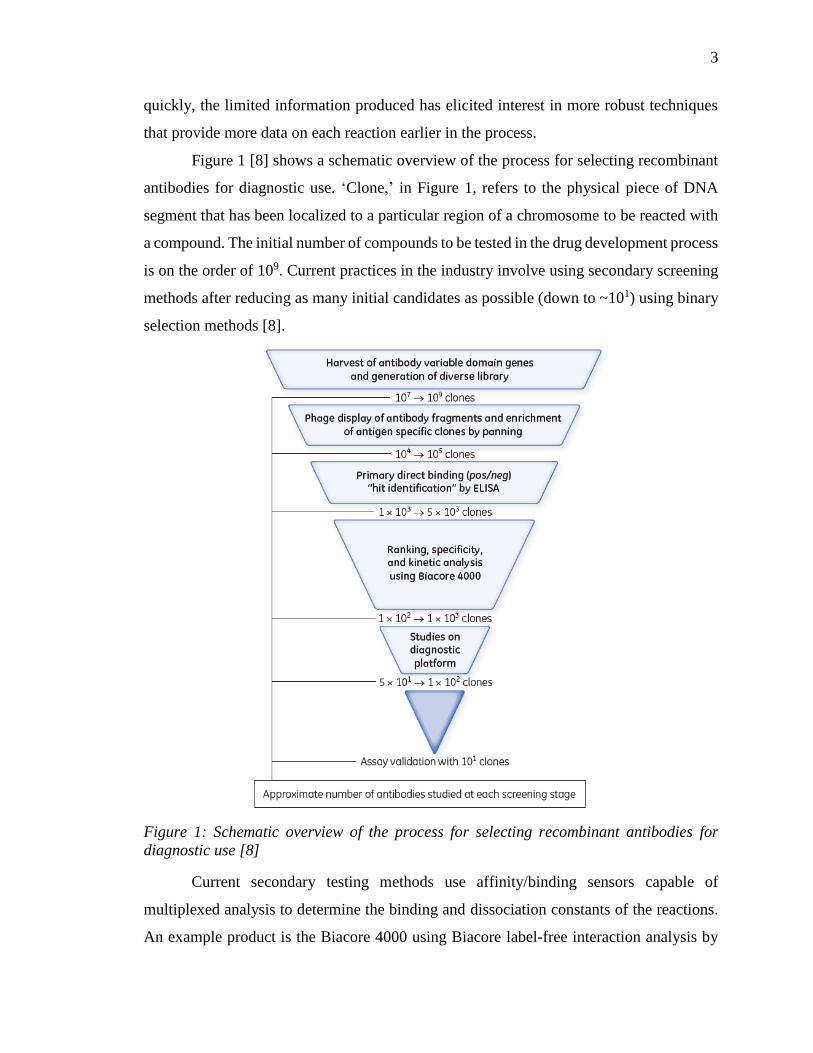
Figure 1 [8] shows a schematic overview of the process for selecting recombinant

antibodies for diagnostic use. ‘Clone,’ in Figure 1, refers to the physical piece of DNA

segment that has been localized to a particular region of a chromosome to be reacted with

a compound. The initial number of compounds to be tested in the drug development process

is on the order of 109. Current practices in the industry involve using secondary screening

methods after reducing as many initial candidates as possible (down to ~101) using binary

selection methods [8].

Figure 1: Schematic overview of the process for selecting recombinant antibodies for

diagnostic use [8]

Current secondary testing methods use affinity/binding sensors capable of

multiplexed analysis to determine the binding and dissociation constants of the reactions.

An example product is the Biacore 4000 using Biacore label-free interaction analysis by

4

GE Healthcare. These sensors use Surface Plasmon Resonance (SPR) to achieve

multiplexed sensing with high sensitivity [8] [9]. These affinity sensors, however, do not

provide enough information on the binding parameters of the reactions due to the binding

affinities between the candidate compounds being too similar. This presents difficulties

when attempting to decide which compounds to select for further testing, making the data

produced by the HTS method very valuable.

Current research in instrument development in the industry focuses on multiplexing

capability, detailed information regarding the interaction kinetics, and shorter run times

[1]. Considering the number of compounds used in each stage of the process, minimization

of protein consumption is very important. One way of accomplishing this is by increasing

the sensitivity of the sensing technologies, so that reaction characteristics may be analyzed

with the least amount of compound while obtaining the most information (such as the

thermodynamic data). Apart from the development of new biosensor technologies,

researchers are also developing new methods to enhance the throughput of existing

biosensors for kinetic screening, however this is beyond the scope of this study [9].

To meet the need for a fast response, multiplexed sensor which can provide detailed

information regarding the reaction kinetics, the calorimeter device using SPR was created

[4] by the Microfluidics Laboratory at Northeastern University. Calorimetry provides

detailed characterization of the thermodynamics of binding interactions, which is an

essential part of the drug design process [10].

Thermodynamic studies of biological processes focus on molecular recognition and

macromolecular stability. Understanding the thermodynamics exposes the nature of the

energetic forces that drive structure and formation. These studies also reveal the

contributions of specific molecular interactions and their variation with temperature, pH,

and ionic strength. Therefore, thermodynamic studies provide detailed information that is

of great value to the fields of biotechnology, medicine and drug design [1]. Calorimetry

can meet all these thermodynamic needs [11].

Most thermodynamic studies begin with experimental determination of the

association/binding constant, Kb [11]. The Gibbs free energy, ΔG, of the process can be

found using Equation (2.1).

𝛥𝐺 = −𝑅𝑇 𝑙𝑛 𝐾𝑏 ( 2.1)

5

where R is the gas constant and T is the absolute temperature of the in Kelvin. Kb

is the reciprocal of the dissociation constant, Kd, found from Equation (2.2).

𝐾𝑑 = 1𝐾𝑏

⁄ ( 2.2)

For detailed thermodynamic study it is necessary to measure the temperature

dependence of the free energy change, found from the change in enthalpy, ΔH, of the

reaction. The enthalpic change is a direct measure of the net change in the number and/or

strength of the non-covalent bonds going from the free to the bound state [1]. From this,

the change in entropy, ΔS, can be calculated. Equation (2.3) describes the Gibbs free energy

change of a reaction at any temperature.

𝛥𝐺(𝑇) = 𝛥𝐻(𝑇𝑅) + ∫ 𝛥𝑐𝑝𝑑𝑇𝑇

𝑇𝑅− 𝑇𝛥𝑆(𝑇𝑅) − 𝑇 ∫ 𝛥𝑐𝑝𝑑 𝑙𝑛 𝑇

𝑇

𝑇𝑅 ( 2.3)

(2.3) can be reduced to (2.4) by setting 𝑇 = 𝑇𝑅. Equation (2.4) describes the Gibbs

free energy change of a reaction at constant temperature.

𝛥𝐺 = 𝛥𝐻 − 𝑇𝛥𝑆 ( 2.4)

These detailed thermodynamic terms are essential to understanding the interaction

between a candidate drug and ligand. Two interactions with similar affinities and structure

can have different enthalpic and entropic contributions to their overall free energies.

Therefore, current HTS methods, like affinity sensors, are unsatisfactory for a detailed

understanding of reaction characteristics. Freire [2] demonstrates how designing

enthalpically optimized drug interactions can distinguish best-in-class from first-in-class

drugs, and suggests these drugs could have been discovered earlier had thermodynamic

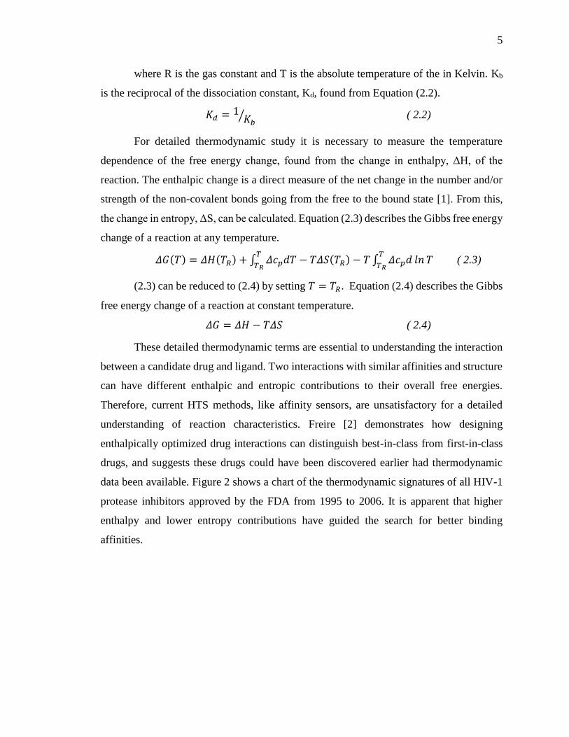
data been available. Figure 2 shows a chart of the thermodynamic signatures of all HIV-1

protease inhibitors approved by the FDA from 1995 to 2006. It is apparent that higher

enthalpy and lower entropy contributions have guided the search for better binding

affinities.

6

Figure 2: Thermodynamic signature of all HIV-1 protease inhibitors approved by the FDA

from 1995 to 2006 [1] [2]

The two major calorimetric techniques discussed in this study are Differential

Scanning Calorimetry (DSC) and Isothermal Titration Calorimetry (ITC). The

instrumentation used for both techniques is very similar, though the setups are different

[12] These techniques are considered complementary: order-disorder transitions, like

protein folding or nucleic acid melting, can be studied with DSC, while ligand-

macromolecule or macromolecule-macromolecule binding can be examined using ITC

[11].

2.1.1 Differential Scanning Calorimetry

Differential Scanning Calorimetry (DSC) is the most direct experimental technique

to resolve the energetics of conformational transitions of biological macromolecules [13].

It is generally accepted as the technique of choice to determine the energetics of protein

folding/unfolding transitions and the underlying thermodynamic mechanisms of those

reactions [14]. DSC is routinely used to study an entire range of biomolecular interactions,

protein stability, lipid phase transitions, surfactant micellization, nucleic acid ‘melts’ and

stability of liquid biopharmaceuticals as well as less defined cellular systems [11]. DSC

measures the apparent molar heat capacity of a substance as a function of temperature. By

manipulating this quantity, the enthalpy of reaction, ΔH, the entropy of reaction, ΔS, and

the heat capacity change, ΔCp, can be obtained [14].

7

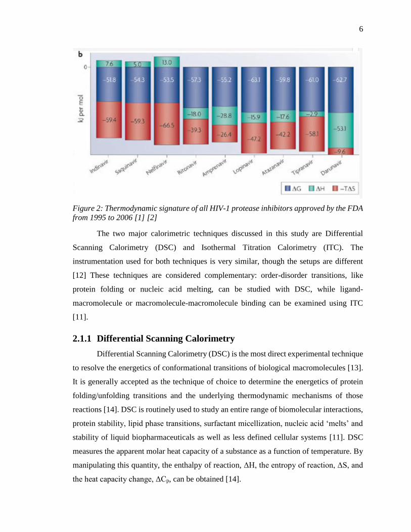
Figure 3: Schematic of Differential Scanning Calorimeter [15]

A DSC instrument contains two cells suspended in an adiabatic jacket and

connected by several heating and temperature/power sensing circuits. During a normal

DSC experiment, the reference cell is filled with buffer while the sample cell is filled with

buffer and macromolecule [11]. A schematic of the experimental setup is shown in Figure

3 [15]. The system is heated (or cooled) quasi-adiabatically at a constant rate, typically

0.5–1.5 K min-1 [13]. Since the heat capacities of the solution in the sample cell and the

solvent in the reference cell differ, a certain amount of electrical power is required to zero

the temperature difference between the two cells. The power difference (J s-1), after

normalization by the scanning rate (K s-1), is a direct measure of the heat capacity

difference between the solution and the solvent [13].

8

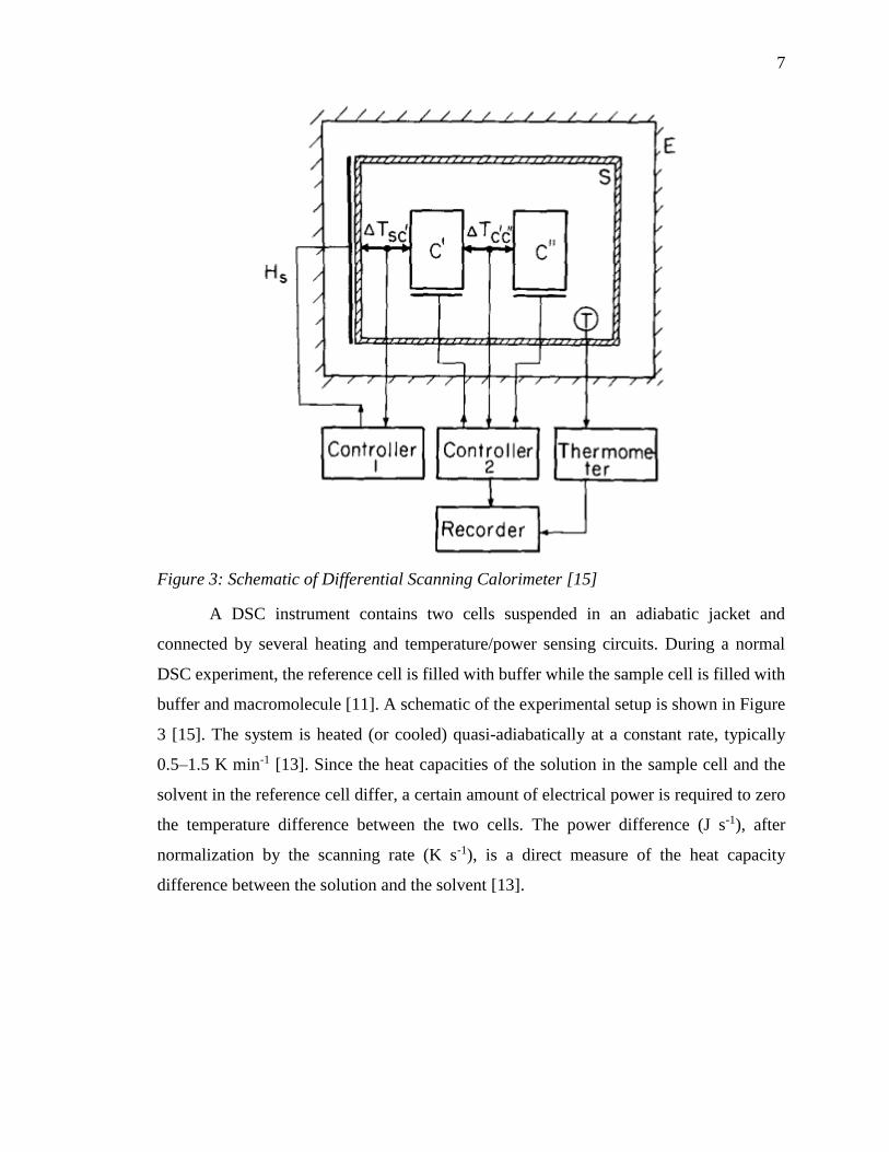
Figure 4: An example DSC trace for the reversible unfolding of a monomeric protein. The

maximum of the heat capacity curve is the Tm and is 60°C. The dashed lines are the linear

extrapolations of the pre- and post-transition baselines into the transition region. The

difference between these values at Tm is the ΔCp. The thick black line is the theoretical

‘progress’ baseline. [11]

Figure 4 shows an example DSC trace for the reversible unfolding of a monomeric

protein. In this figure, the maximum temperature, Tm, of the heat capacity curve is at 60°C.

This is the transition temperature of the process due to the excess heat capacity reaching

its maximum value. The difference in the extrapolated pre- and post-transition baselines at

Tm is the ΔCp of the process. The blue area under the Cp curve and above the theoretical

‘progress’ baseline is the ΔH for the process. Equation (2.5) can be used to calculate the

calorimetric transition enthalpy, ΔH.

𝛥𝐻 = ∫ 𝐶𝑝𝑑𝑇 ( 2.5)

The experimentally obtained heat capacity curve along with the temperature profile

can also be used to calculate the overall entropy change, ΔS, of the process with Equation

(2.6).

𝛥𝑆 = ∫𝐶𝑝

𝑇𝑑𝑇 ( 2.6)

9

Using ΔH and ΔS, the Gibbs free energy change, ΔG, of the process can be

calculated with Equation (2.4).

All Differential Scanning Calorimeters measure heat capacity change continuously

with continuous heating or cooling of the sample at a constant rate. This differs from other

calorimetric devices which measure in a discrete way with discrete energy increments.

Continuous heating and measurement have great advantages over the discrete procedure:

it gives more complete information on the heat capacity function and permits the complete

automatization of all the measurement processes. The only disadvantage is that the studied

sample is never in complete thermal equilibrium, which means certain requirements must

be set for the studied samples [15].

2.1.2 Isothermal Titration Calorimetry

Isothermal Titration Calorimetry (ITC) differs from DSC in that the interaction is

monitored at a constant temperature. ITC is the most direct method to measure the energy

released on formation of a complex at constant temperature [13]. This methodology relies

upon a differential cell system within the calorimeter assembly. The reference cell contains

only water or buffer, while the sample cell contains the macromolecule or ligand and

sometimes a stirring device [11]. The experiment is performed by titrating one binding

partner into the sample cell containing macromolecule or ligand. After each small addition

of the binding partner, the heat released or absorbed in the sample cell is measured with

respect to the reference cell filled with buffer. The heat change is expressed as the electrical

power (J s-1) required to maintain a constant small temperature difference between the

sample cell and the reference cell, which are both placed in an adiabatic jacket [13].

10

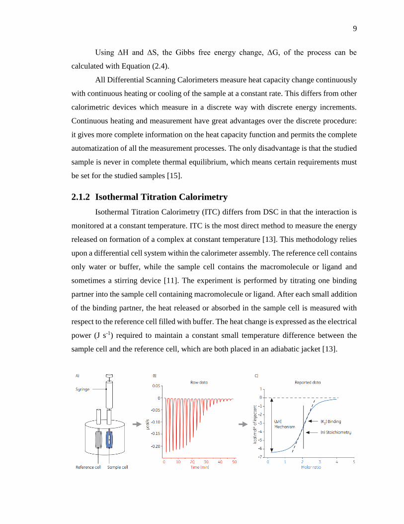
Figure 5: A) Schematic of ITC experimental setup. B) Raw Data captured from ITC

experiment. C) Reported data after analysis to determine binding constant (Kb),

stoichiometry (n) and enthalpy of reaction (ΔH) [16]

ITC is a proficient technique for examining biological interactions because a well-

designed experiment will generate the binding enthalpy (ΔH), the equilibrium binding

constant (Kb) and the reaction stoichiometry (n) in a single two hour experiment. By

performing these experiments over a range of temperatures, the change in heat capacity

(ΔCp) can also be determined [11].

ITC can be used to study almost any bimolecular complex formation with a defined

stoichiometry. The major advantage of ITC is that there is no real assay development and

as such affinities can be determined rapidly for a range of systems with very little prior

knowledge other than sample concentration [11]. The main disadvantages of ITC are the

long experiment time and discrete nature of the experimental procedure. The discrete

titrations can limit the ability for a full understanding of the energetic profile of the reaction.

The Microfluidics Laboratory at Northeastern University focuses on the

development of a calorimeter which uses an ITC approach to calculate ΔH of reactions

based on the phenomena of Surface Plasmon Resonance (SPR) and Extraordinary Optical

Transmission (EOT). The literature on SPR and EOT is presented in the following section.

2.2 SURFACE PLASMON RESONANCE AND EXTRAORDINARY

OPTICAL TRANSMISSION

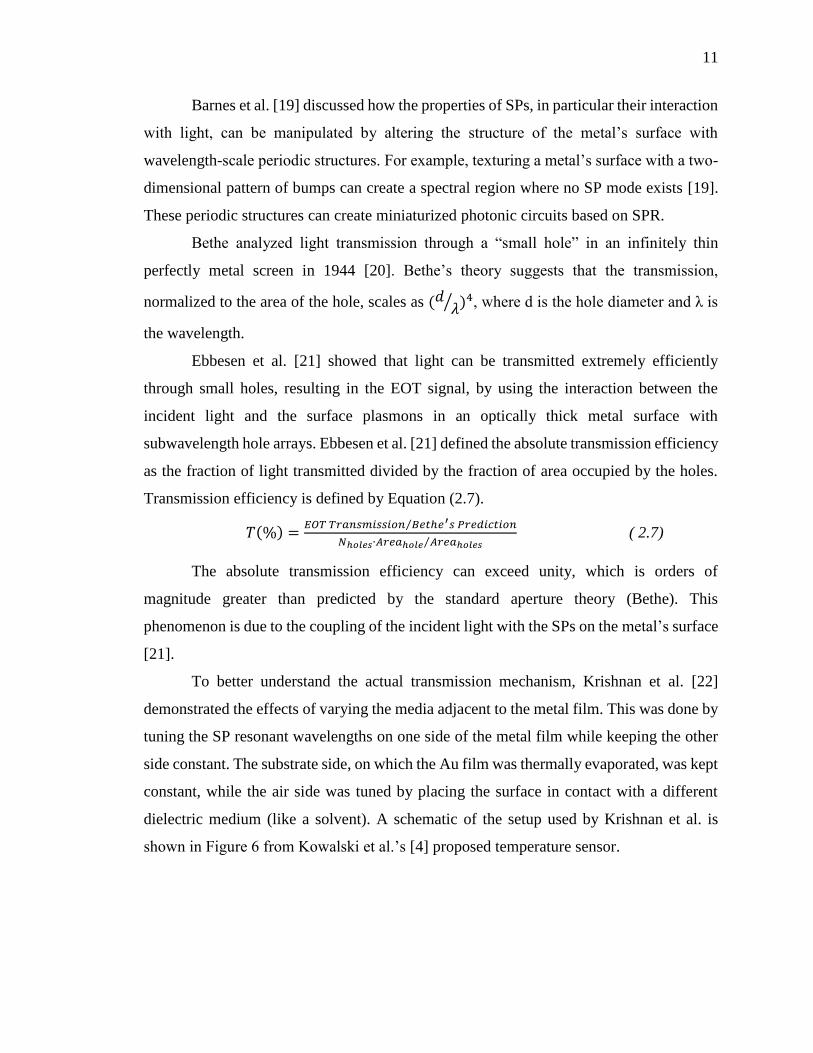
Intensive research has been performed in the fields of Surface Plasmon Resonance

(SPR) and Extraordinary Optical Transmission (EOT) since the discovery of Surface

Plasmons by Ritchie in 1957 [17]. In 2008, Coe et al. [18] conducted an extensive review

of the literature on SPR and EOT.

Surface plasmons (SP) are, essentially, light trapped at a metal’s surface by its

interaction with the metal’s conducting electrons, which act like a plasma [18]. The

incident light excites an oscillation of the electron clouds localized on the metal surface.

Such excitations can be transferred to similar, adjacent structures if they are sufficiently

close. Periodic arrays of coupled particles enable excitations to propagate along the arrays

like ripples on a pond [18].

11

Barnes et al. [19] discussed how the properties of SPs, in particular their interaction

with light, can be manipulated by altering the structure of the metal’s surface with

wavelength-scale periodic structures. For example, texturing a metal’s surface with a two-

dimensional pattern of bumps can create a spectral region where no SP mode exists [19].

These periodic structures can create miniaturized photonic circuits based on SPR.

Bethe analyzed light transmission through a “small hole” in an infinitely thin

perfectly metal screen in 1944 [20]. Bethe’s theory suggests that the transmission,

normalized to the area of the hole, scales as (𝑑𝜆⁄ )4, where d is the hole diameter and λ is

the wavelength.

Ebbesen et al. [21] showed that light can be transmitted extremely efficiently

through small holes, resulting in the EOT signal, by using the interaction between the

incident light and the surface plasmons in an optically thick metal surface with

subwavelength hole arrays. Ebbesen et al. [21] defined the absolute transmission efficiency

as the fraction of light transmitted divided by the fraction of area occupied by the holes.

Transmission efficiency is defined by Equation (2.7).

𝑇(%) =𝐸𝑂𝑇 𝑇𝑟𝑎𝑛𝑠𝑚𝑖𝑠𝑠𝑖𝑜𝑛 𝐵𝑒𝑡ℎ𝑒′𝑠 𝑃𝑟𝑒𝑑𝑖𝑐𝑡𝑖𝑜𝑛⁄

𝑁ℎ𝑜𝑙𝑒𝑠∙𝐴𝑟𝑒𝑎ℎ𝑜𝑙𝑒 𝐴𝑟𝑒𝑎ℎ𝑜𝑙𝑒𝑠⁄ ( 2.7)

The absolute transmission efficiency can exceed unity, which is orders of

magnitude greater than predicted by the standard aperture theory (Bethe). This

phenomenon is due to the coupling of the incident light with the SPs on the metal’s surface

[21].

To better understand the actual transmission mechanism, Krishnan et al. [22]

demonstrated the effects of varying the media adjacent to the metal film. This was done by

tuning the SP resonant wavelengths on one side of the metal film while keeping the other

side constant. The substrate side, on which the Au film was thermally evaporated, was kept

constant, while the air side was tuned by placing the surface in contact with a different

dielectric medium (like a solvent). A schematic of the setup used by Krishnan et al. is

shown in Figure 6 from Kowalski et al.’s [4] proposed temperature sensor.

12

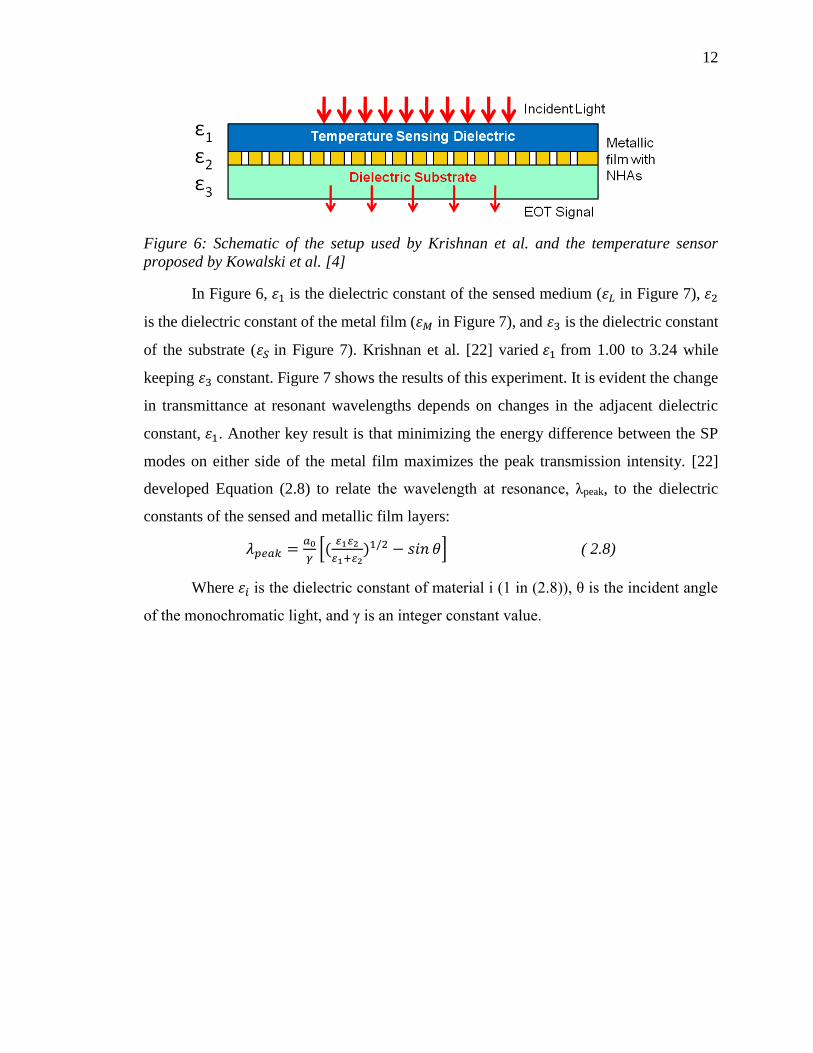
Figure 6: Schematic of the setup used by Krishnan et al. and the temperature sensor

proposed by Kowalski et al. [4]

In Figure 6, 𝜀1 is the dielectric constant of the sensed medium (𝜀𝐿 in Figure 7), 𝜀2

is the dielectric constant of the metal film (𝜀𝑀 in Figure 7), and 𝜀3 is the dielectric constant

of the substrate (𝜀𝑆 in Figure 7). Krishnan et al. [22] varied 𝜀1 from 1.00 to 3.24 while

keeping 𝜀3 constant. Figure 7 shows the results of this experiment. It is evident the change

in transmittance at resonant wavelengths depends on changes in the adjacent dielectric

constant, 𝜀1. Another key result is that minimizing the energy difference between the SP

modes on either side of the metal film maximizes the peak transmission intensity. [22]

developed Equation (2.8) to relate the wavelength at resonance, λpeak, to the dielectric

constants of the sensed and metallic film layers:

𝜆𝑝𝑒𝑎𝑘 =𝑎0

𝛾[(

𝜀1𝜀2

𝜀1+𝜀2)1/2 − 𝑠𝑖𝑛 𝜃] ( 2.8)

Where 𝜀𝑖 is the dielectric constant of material i (1 in (2.8)), θ is the incident angle

of the monochromatic light, and γ is an integer constant value.

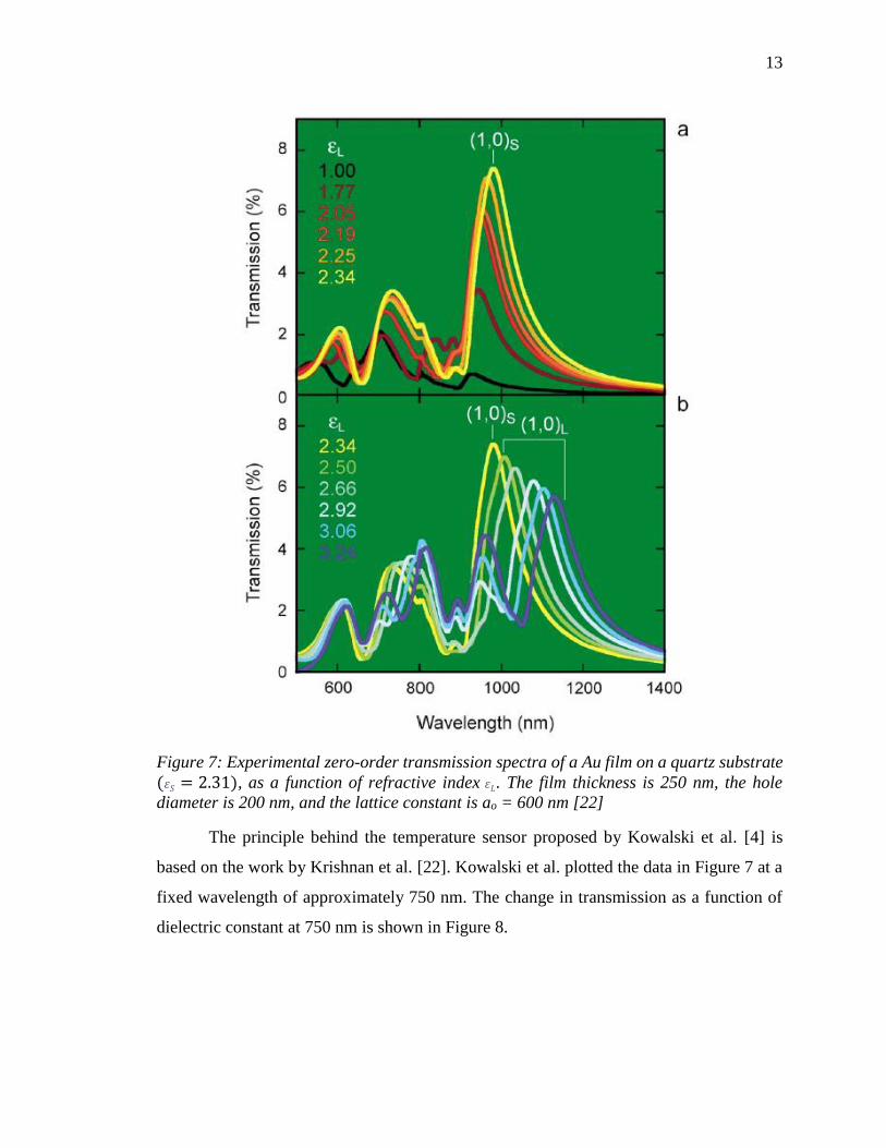
13

Figure 7: Experimental zero-order transmission spectra of a Au film on a quartz substrate

(𝜀𝑆 = 2.31), as a function of refractive index 𝜀𝐿. The film thickness is 250 nm, the hole

diameter is 200 nm, and the lattice constant is ao = 600 nm [22]

The principle behind the temperature sensor proposed by Kowalski et al. [4] is

based on the work by Krishnan et al. [22]. Kowalski et al. plotted the data in Figure 7 at a

fixed wavelength of approximately 750 nm. The change in transmission as a function of

dielectric constant at 750 nm is shown in Figure 8.

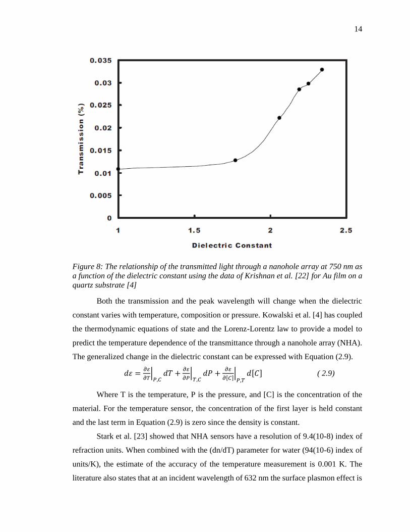
14

Figure 8: The relationship of the transmitted light through a nanohole array at 750 nm as

a function of the dielectric constant using the data of Krishnan et al. [22] for Au film on a

quartz substrate [4]

Both the transmission and the peak wavelength will change when the dielectric

constant varies with temperature, composition or pressure. Kowalski et al. [4] has coupled

the thermodynamic equations of state and the Lorenz-Lorentz law to provide a model to

predict the temperature dependence of the transmittance through a nanohole array (NHA).

The generalized change in the dielectric constant can be expressed with Equation (2.9).

𝑑𝜀 =𝜕𝜀

𝜕𝑇|

𝑃,𝐶𝑑𝑇 +

𝜕𝜀

𝜕𝑃|

𝑇,𝐶𝑑𝑃 +

𝜕𝜀

𝜕[𝐶]|

𝑃,𝑇𝑑[𝐶] ( 2.9)

Where T is the temperature, P is the pressure, and [C] is the concentration of the

material. For the temperature sensor, the concentration of the first layer is held constant

and the last term in Equation (2.9) is zero since the density is constant.

Stark et al. [23] showed that NHA sensors have a resolution of 9.4(10-8) index of

refraction units. When combined with the (dn/dT) parameter for water (94(10-6) index of

units/K), the estimate of the accuracy of the temperature measurement is 0.001 K. The

literature also states that at an incident wavelength of 632 nm the surface plasmon effect is

15

limited to 100 nm above the NHA sensor. This sensitivity and small sensor volume

illustrate the sensitivity and resolution of the NHA sensors. Lastly, due to their interaction

with light, their response time is on the order of speed of light [5].

2.3 CURRENT APPROACH/PREVIOUS WORK

This section details the current approach used to collect EOT data as well as

previous work done in DSC and ITC in the laboratory.

2.3.1 Experimental Setup

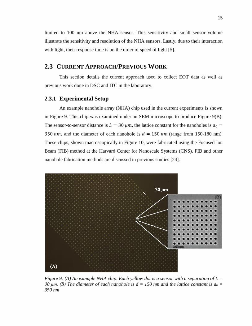
An example nanohole array (NHA) chip used in the current experiments is shown

in Figure 9. This chip was examined under an SEM microscope to produce Figure 9(B).

The sensor-to-sensor distance is 𝐿 = 30 𝜇𝑚, the lattice constant for the nanoholes is 𝑎0 =

350 𝑛𝑚, and the diameter of each nanohole is 𝑑 = 150 𝑛𝑚 (range from 150-180 nm).

These chips, shown macroscopically in Figure 10, were fabricated using the Focused Ion

Beam (FIB) method at the Harvard Center for Nanoscale Systems (CNS). FIB and other

nanohole fabrication methods are discussed in previous studies [24].

Figure 9: (A) An example NHA chip. Each yellow dot is a sensor with a separation of L =

30 μm. (B) The diameter of each nanohole is d = 150 nm and the lattice constant is a0 =

350 nm

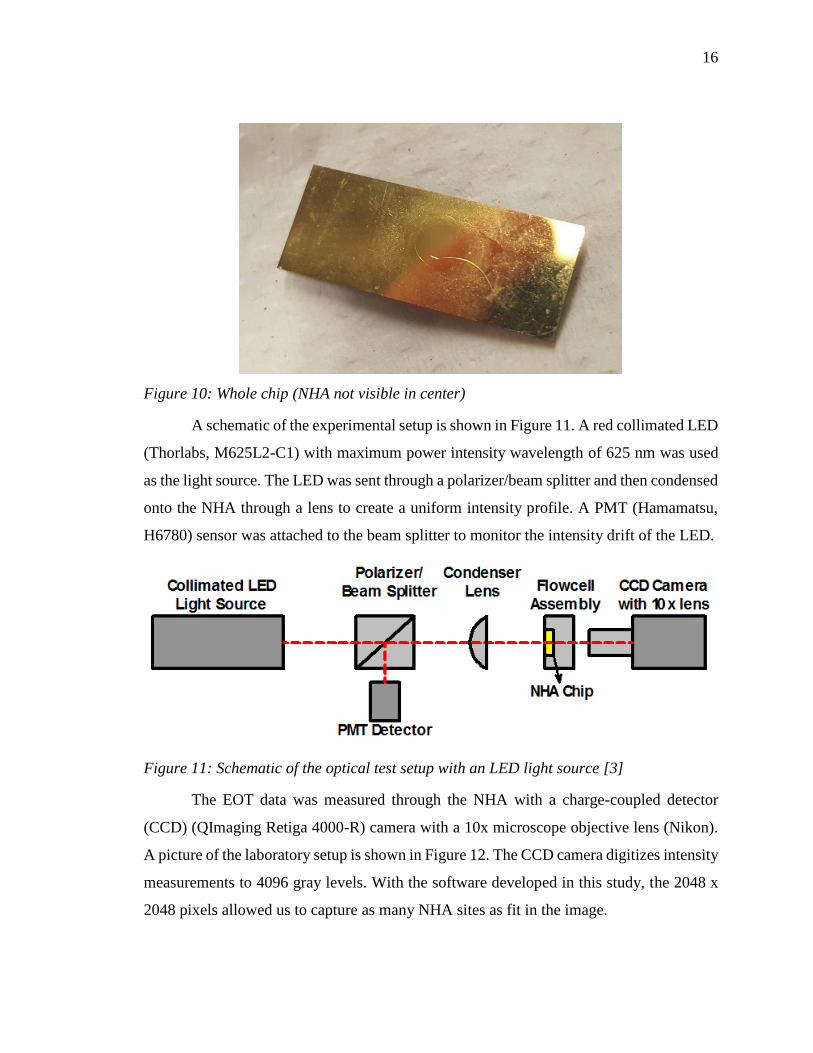
16

Figure 10: Whole chip (NHA not visible in center)

A schematic of the experimental setup is shown in Figure 11. A red collimated LED

(Thorlabs, M625L2-C1) with maximum power intensity wavelength of 625 nm was used

as the light source. The LED was sent through a polarizer/beam splitter and then condensed

onto the NHA through a lens to create a uniform intensity profile. A PMT (Hamamatsu,

H6780) sensor was attached to the beam splitter to monitor the intensity drift of the LED.

Figure 11: Schematic of the optical test setup with an LED light source [3]

The EOT data was measured through the NHA with a charge-coupled detector

(CCD) (QImaging Retiga 4000-R) camera with a 10x microscope objective lens (Nikon).

A picture of the laboratory setup is shown in Figure 12. The CCD camera digitizes intensity

measurements to 4096 gray levels. With the software developed in this study, the 2048 x

2048 pixels allowed us to capture as many NHA sites as fit in the image.

17

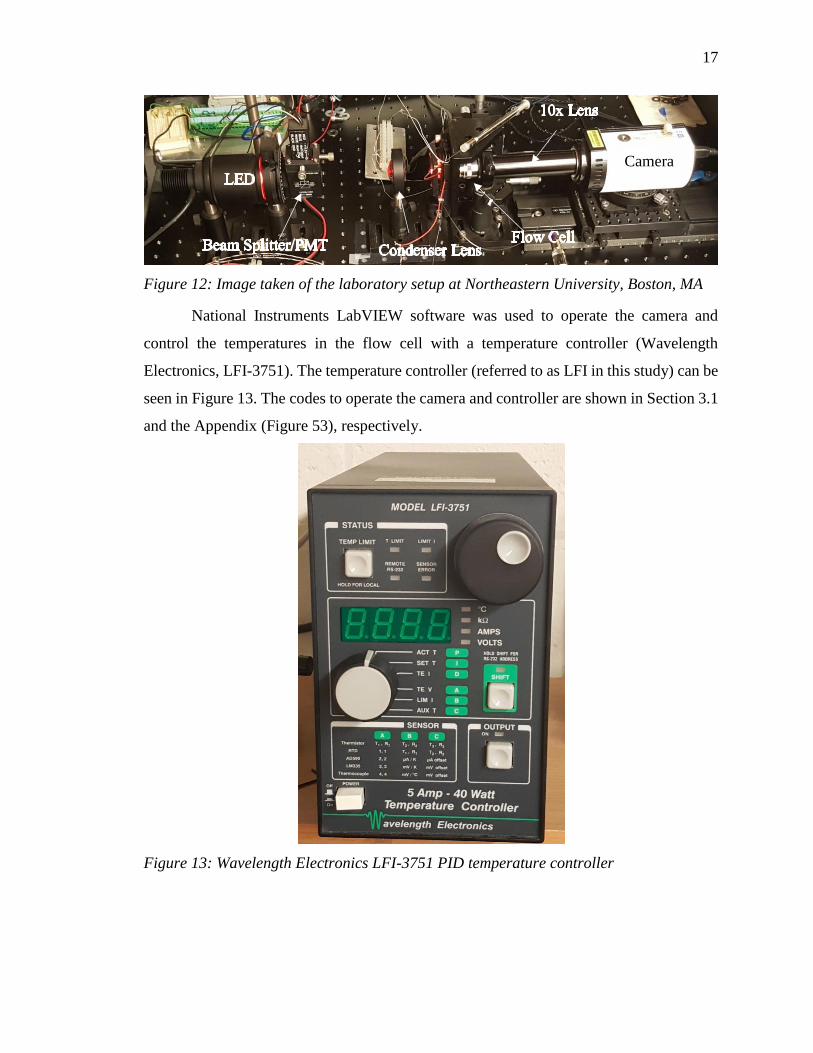
Figure 12: Image taken of the laboratory setup at Northeastern University, Boston, MA

National Instruments LabVIEW software was used to operate the camera and

control the temperatures in the flow cell with a temperature controller (Wavelength

Electronics, LFI-3751). The temperature controller (referred to as LFI in this study) can be

seen in Figure 13. The codes to operate the camera and controller are shown in Section 3.1

and the Appendix (Figure 53), respectively.

Figure 13: Wavelength Electronics LFI-3751 PID temperature controller

Camera

18

2.3.1.1 Flow Cell

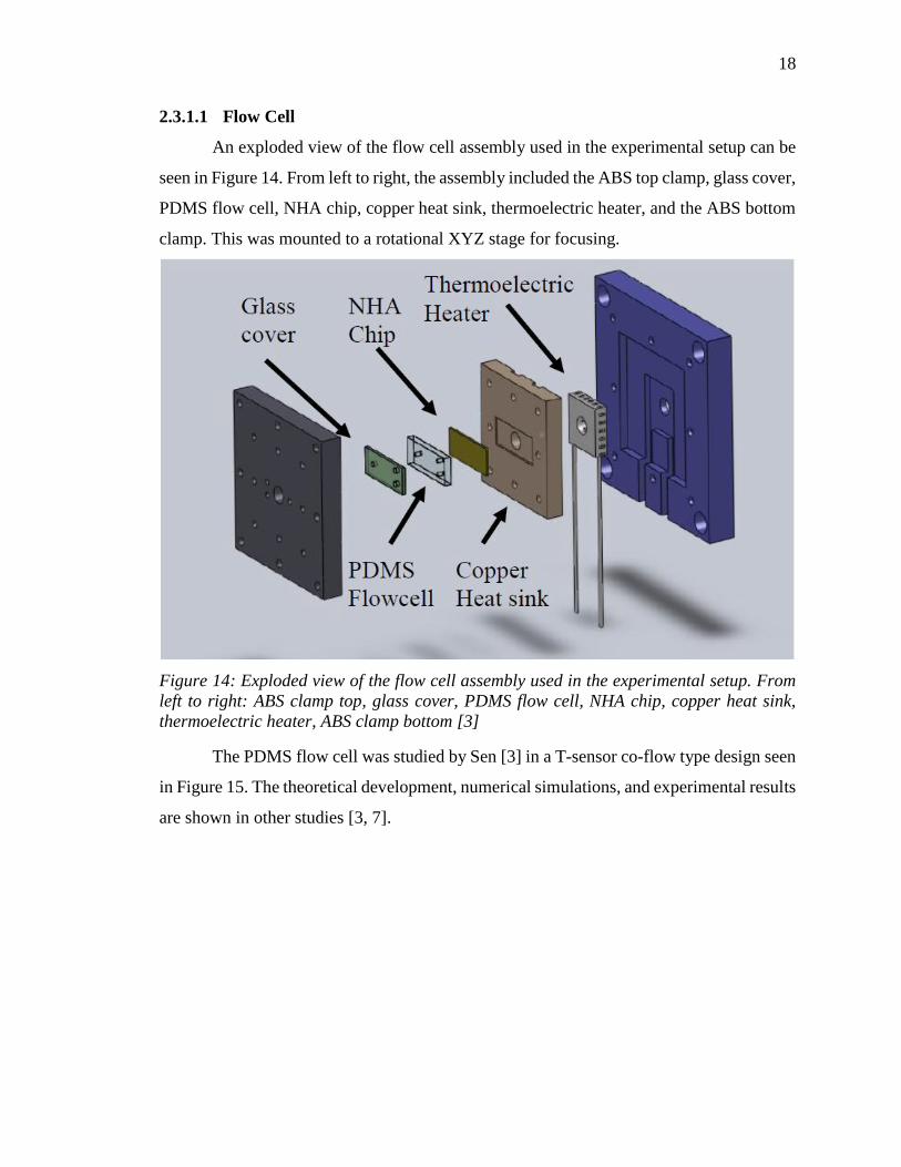
An exploded view of the flow cell assembly used in the experimental setup can be

seen in Figure 14. From left to right, the assembly included the ABS top clamp, glass cover,

PDMS flow cell, NHA chip, copper heat sink, thermoelectric heater, and the ABS bottom

clamp. This was mounted to a rotational XYZ stage for focusing.

Figure 14: Exploded view of the flow cell assembly used in the experimental setup. From

left to right: ABS clamp top, glass cover, PDMS flow cell, NHA chip, copper heat sink,

thermoelectric heater, ABS clamp bottom [3]

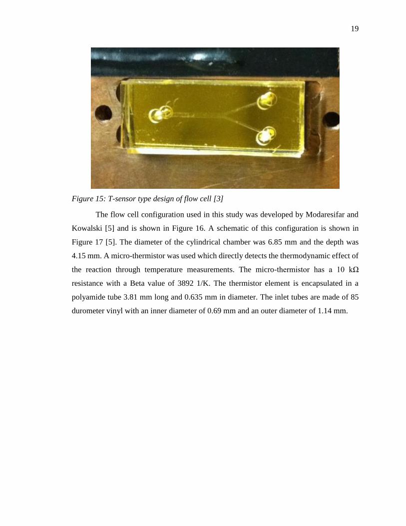
The PDMS flow cell was studied by Sen [3] in a T-sensor co-flow type design seen

in Figure 15. The theoretical development, numerical simulations, and experimental results

are shown in other studies [3, 7].

19

Figure 15: T-sensor type design of flow cell [3]

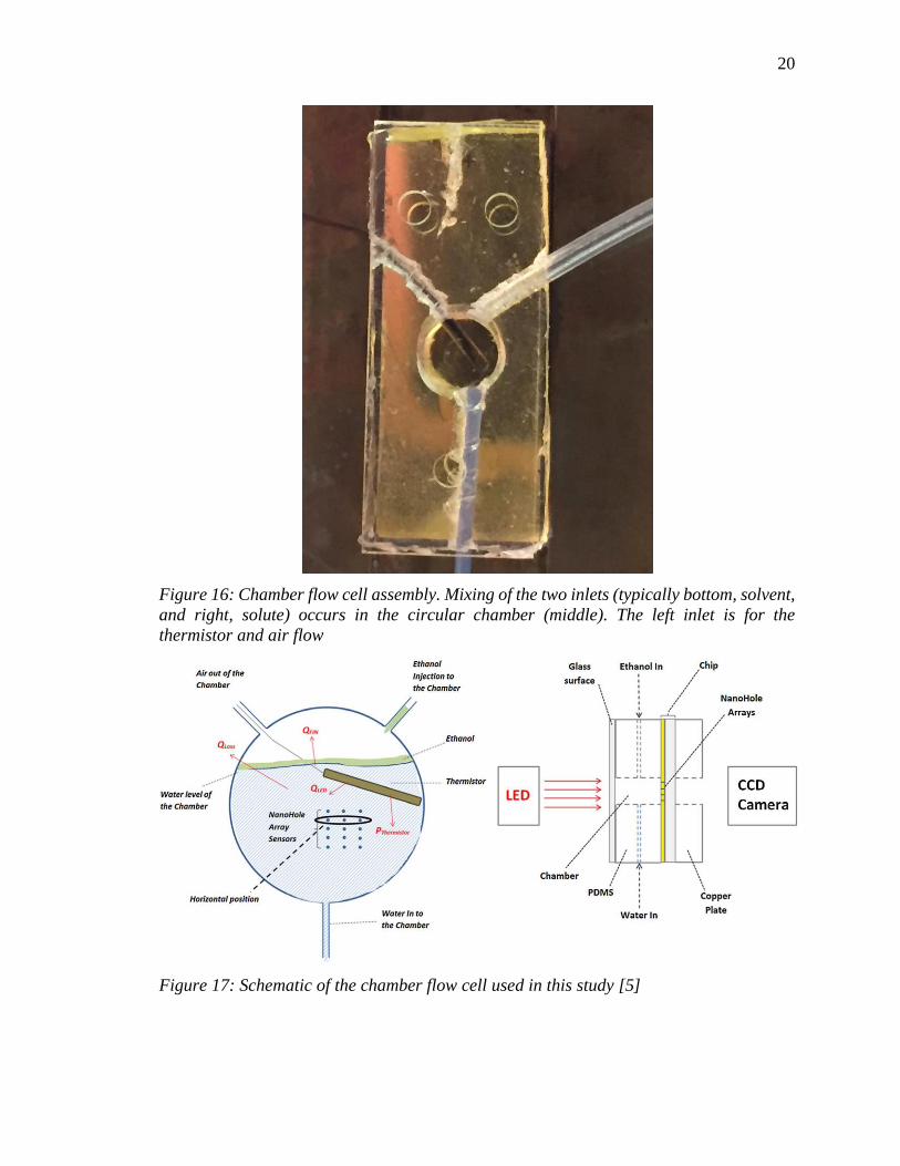
The flow cell configuration used in this study was developed by Modaresifar and

Kowalski [5] and is shown in Figure 16. A schematic of this configuration is shown in

Figure 17 [5]. The diameter of the cylindrical chamber was 6.85 mm and the depth was

4.15 mm. A micro-thermistor was used which directly detects the thermodynamic effect of

the reaction through temperature measurements. The micro-thermistor has a 10 kΩ

resistance with a Beta value of 3892 1/K. The thermistor element is encapsulated in a

polyamide tube 3.81 mm long and 0.635 mm in diameter. The inlet tubes are made of 85

durometer vinyl with an inner diameter of 0.69 mm and an outer diameter of 1.14 mm.

20

Figure 16: Chamber flow cell assembly. Mixing of the two inlets (typically bottom, solvent,

and right, solute) occurs in the circular chamber (middle). The left inlet is for the

thermistor and air flow

Figure 17: Schematic of the chamber flow cell used in this study [5]

21

2.3.2 Sensor Location Method

The Sensor Location Method is the current method used in the laboratory. It follows

an ITC approach as described by Modaresifar and Kowalski [5] and Sen [3]. A LabVIEW

program is used to collect EOT data from sensor locations inputted prior to the experiment.

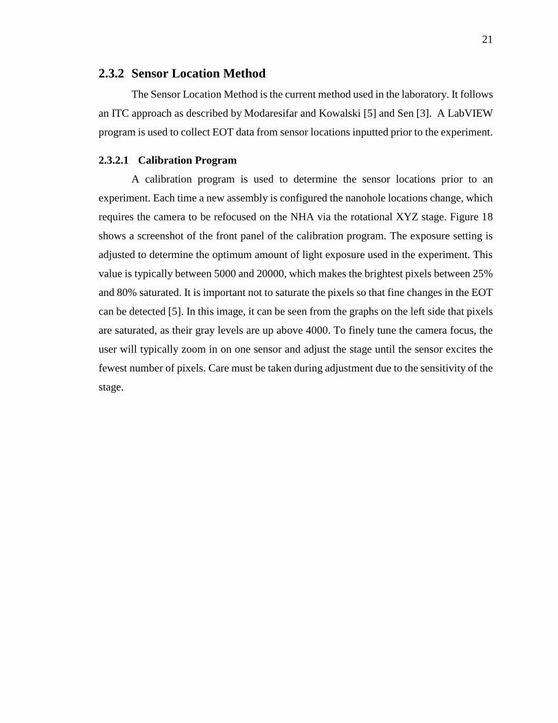
2.3.2.1 Calibration Program

A calibration program is used to determine the sensor locations prior to an

experiment. Each time a new assembly is configured the nanohole locations change, which

requires the camera to be refocused on the NHA via the rotational XYZ stage. Figure 18

shows a screenshot of the front panel of the calibration program. The exposure setting is

adjusted to determine the optimum amount of light exposure used in the experiment. This

value is typically between 5000 and 20000, which makes the brightest pixels between 25%

and 80% saturated. It is important not to saturate the pixels so that fine changes in the EOT

can be detected [5]. In this image, it can be seen from the graphs on the left side that pixels

are saturated, as their gray levels are up above 4000. To finely tune the camera focus, the

user will typically zoom in on one sensor and adjust the stage until the sensor excites the

fewest number of pixels. Care must be taken during adjustment due to the sensitivity of the

stage.

22

Figure 18: Front panel of the calibration program used to determine the sensor locations

prior to an experiment. Exposure of 50000 saturates the camera.

2.3.2.2 Program Characteristics

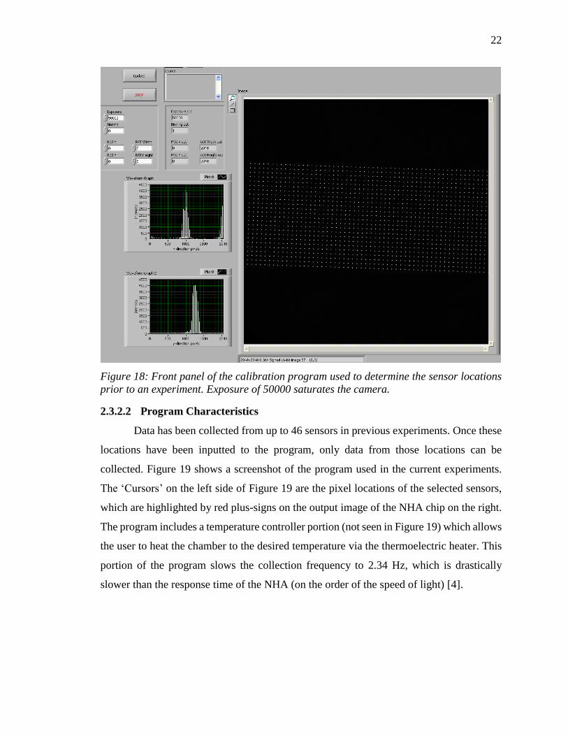
Data has been collected from up to 46 sensors in previous experiments. Once these

locations have been inputted to the program, only data from those locations can be

collected. Figure 19 shows a screenshot of the program used in the current experiments.

The ‘Cursors’ on the left side of Figure 19 are the pixel locations of the selected sensors,

which are highlighted by red plus-signs on the output image of the NHA chip on the right.

The program includes a temperature controller portion (not seen in Figure 19) which allows

the user to heat the chamber to the desired temperature via the thermoelectric heater. This

portion of the program slows the collection frequency to 2.34 Hz, which is drastically

slower than the response time of the NHA (on the order of the speed of light) [4].

23

Figure 19: A screenshot of the current program used in the laboratory to collect EOT data.

The 'Cursors' shown on the left side are the pixel locations of the selected sensors, which

are highlighted by red plus-signs on the right side in the NHA output image

2.3.2.3 Drawbacks

The issues with the Sensor Location Method lie in the inherent characteristics of a

calorimetric test (especially at such small volumes): changes in temperature and system

response time.

As the cell assemblies are heated or cooled they will expand or contract. By

monitoring data at specific pixel locations which cannot fluctuate with the location

changes, the tests can be impossible to conduct or produce inadequate data. Figure 21

below shows a sensors intensity by pixel captured by the CCD camera. As the temperature

rises, the sensor will move outside the area targeted by the camera, hence the need for

dynamic monitoring of sensors.

ITC tests are often conducted over longer periods of time due to the nature of the

periodic solute additions. The Sensor Location Method can handle these longer tests as

long as the temperature changes due the reactions aren’t too great to disrupt the data

collection locations. DSC, however, can provide a more complete view of the

thermodynamics of the system by continuously collecting data during the scanning of the

temperature profile. These tests require a new method which can monitor EOT at changing

24

locations and provide a collection frequency high enough to capture the speed of the

reaction energetics. This new method is the topic of this thesis and is outlined in Section 3.

2.3.3 Previous DSC Work

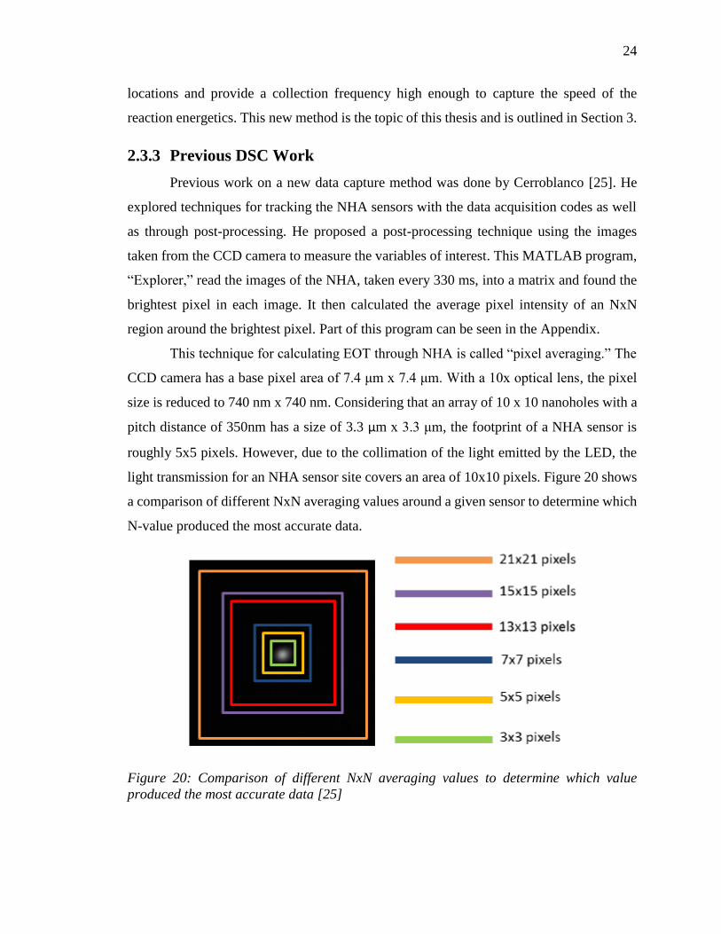
Previous work on a new data capture method was done by Cerroblanco [25]. He

explored techniques for tracking the NHA sensors with the data acquisition codes as well

as through post-processing. He proposed a post-processing technique using the images

taken from the CCD camera to measure the variables of interest. This MATLAB program,

“Explorer,” read the images of the NHA, taken every 330 ms, into a matrix and found the

brightest pixel in each image. It then calculated the average pixel intensity of an NxN

region around the brightest pixel. Part of this program can be seen in the Appendix.

This technique for calculating EOT through NHA is called “pixel averaging.” The

CCD camera has a base pixel area of 7.4 μm x 7.4 μm. With a 10x optical lens, the pixel

size is reduced to 740 nm x 740 nm. Considering that an array of 10 x 10 nanoholes with a

pitch distance of 350nm has a size of 3.3 μm x 3.3 μm, the footprint of a NHA sensor is

roughly 5x5 pixels. However, due to the collimation of the light emitted by the LED, the

light transmission for an NHA sensor site covers an area of 10x10 pixels. Figure 20 shows

a comparison of different NxN averaging values around a given sensor to determine which

N-value produced the most accurate data.

Figure 20: Comparison of different NxN averaging values to determine which value

produced the most accurate data [25]

25

Figure 21: EOT intensity from each pixel in an image with a 13x13 pixel area [25]

The 13x13 pixel average was determined to be most accurate due to the high

sensitivity and complete sensor coverage [25]. Figure 21 shows EOT intensity from each

pixel in an image of a sensor with a 13x13 pixel area. While these discoveries were

beneficial to data analysis through post-processing, “Explorer” failed to address sensor

tracking from temperature change or analysis of more than one sensor. These parameters

are essential to a temperature sensor for an application like DSC. This study focuses on the

development of post-processing programs to track multiple sensors simultaneously, while

increasing collection frequency to capture fast reaction energetics.

3 APPROACH AND METHODS

To improve the highly sensitive, accurate temperature sensor from EOT though an

NHA, the following is proposed: An image capturing program to collect data during

experiments and a post-processing program to calculate EOT from all sensors seen in the

captured images. This is called the Full Field Image Capture Method.

26

3.1 IMAGE CAPTURE PROGRAMS

3.1.1 Basic Capture Program

To capture images of the NHA chip during an experiment, an image capturing

program was developed in LabVIEW. Figures 22a and 22b show screenshots of the front

panel and the block diagram of the Basic Image Capture LabVIEW virtual-instrument (VI),

respectively. This program had a maximum calculated capture speed of 3.63 Hz with full

2048 x 2048 pixel images. The program was developed with preloaded LabVIEW VIs from

the manufacturer and specialized for the laboratory’s purposes. Due to its rudimentary

nature, the Basic Image Capture VI was only used in preliminary experiments discussed in

Section 4. It served as a benchmark for the Region-of-Interest Control Edition and the

Temperature Control Edition. C++ was investigated as another language to operate the

system but time constraints and previous work discussed in Section 2.3 made LabVIEW

the better choice. Future work with C++ is discussed in Section 6.

Figure 22: a) front panel of the Basic Image Capture VI, b) block diagram

3.1.1.1 Construction

Construction of the data collection aspect of the program was primarily based on

ease of transferability to the MATLAB post-processing programs. Tagged Image File

Format (TIFF) was chosen as the saved image format because of the uncompressed nature

of the file. Preservation of the integrity of the image is essential due to the sensitivity of

the gray level changes between consecutive images, making it dangerous to compress the

images in any format. The general nature of TIFF allows it to be used in any operating

a)

b)

27

environment, and it is found on most platforms requiring image data storage [26]. The

images were saved consecutively in an ‘ImageX’ format where X represents the loop

iteration, or image number, captured during the experiment. It saved data to a specific

folder in the laboratory computer and overwrote all data with the same names automatically

so that the user didn’t need to erase all data previously in the folder. This also limits space

used by the program in the capture computer. This folder was located here: C:\Documents

and Settings\Tom\Desktop\Data\Nanohole_Captures. A “Wait” block was added to the

program so that a frequency slower than the max could be achieved, if desired. Finally, a

timer and frequency indicator were added for analysis.

Figure 23: 2048 x 2048 image captured during an experiment in May 2017. The shadow

on the left of the image is the thermistor overlapping the NHA in the chamber.

28

Figure 23 shows an example 2048 x 2048 pixel image captured in an experiment

from May 2017. Each one of the white dots in the image is one sensor, similar to Figure

9a. Each sensor consists of a 10x10 NHA, as seen in Figure 9b. The shadow covering the

sensors on the left is the thermistor overlapping the NHA chip in the chamber. In this

image, the array is seen tilted from the normal; this is due to the size of the assembly

making it difficult to align the chip perfectly. This happens frequently and analysis methods

had to be created to deal with this issue.

3.1.1.2 Procedure

The Basic Image Capture program was created to be easy to use and operate. For

example, the user would construct an experiment by filling the chamber with a solvent and

heating the chamber to a desired temperature via a power supply. The user would then open

and run the program and subsequently inject the solute. When the process or reaction was

complete, the user would stop the program. This would capture the EOT data (consecutive

2048 x 2048 images) for the entirety of the experiment and the EOT could be analyzed

with the post-processing programs discussed in Section 3.2.

To run another experiment, the user must close the program and restart the camera.

This is due to the “IMAQ Write File 2 VI” running into an unknown issue when it attempts

to resave over previously saved images.

3.1.2 Region-of-Interest Control Edition

The CCD camera used in the experimental setup has a maximum rated capture

speed of 125 frames per second (fps) with a 1x1 pixel region of interest (ROI). As stated

in Section 3.1, the Basic Image Capture VI had a capture speed of 3.63 Hz with full 2048

x 2048 pixel images. To increase the capture rate of the base program, the ROI had to be

diminished, and hence another iteration of the base program was created with an ROI

element added. Figure 24 shows a screenshot of the front panel of the ROI Control Edition

VI.

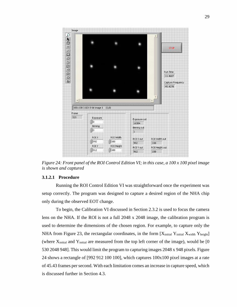
29

Figure 24: Front panel of the ROI Control Edition VI; in this case, a 100 x 100 pixel image

is shown and captured

3.1.2.1 Procedure

Running the ROI Control Edition VI was straightforward once the experiment was

setup correctly. The program was designed to capture a desired region of the NHA chip

only during the observed EOT change.

To begin, the Calibration VI discussed in Section 2.3.2 is used to focus the camera

lens on the NHA. If the ROI is not a full 2048 x 2048 image, the calibration program is

used to determine the dimensions of the chosen region. For example, to capture only the

NHA from Figure 23, the rectangular coordinates, in the form [Xinitial Yinitial Xwidth Yheight]

(where Xinitial and Yinitial are measured from the top left corner of the image), would be [0

530 2048 948]. This would limit the program to capturing images 2048 x 948 pixels. Figure

24 shows a rectangle of [992 912 100 100], which captures 100x100 pixel images at a rate

of 45.43 frames per second. With each limitation comes an increase in capture speed, which

is discussed further in Section 4.3.

30

3.1.3 Temperature Control Edition

To test the validity of the Full Field Image Capture Method, the collected EOT data

was to be compared to temperature data. To collect temperature data while simultaneously

capturing images, the LFI temperature controller VI was added to the Basic Image Capture

VI. Due to the LFI’s hard code, the maximum capture speed was reduced to 1 Hz. Attempts

were made to increase this capture speed but to no avail. It was determined that a different

temperature control system would be needed to increase the capture speed. Figure 25 shows

a screenshot of the front panel of the capture VI with temperature control. The block

diagram of the Temperature Control Edition can be found in the Appendix.

Figure 25: Front panel of the Temperature Control Edition

3.1.3.1 Procedure

Running the Temperature Control Edition VI was slightly more complicated than

the base program due to the abilities of the temperature controller. The user began by

setting up the chamber assembly to be tested and opening the base LFI VI (not the

Temperature Control Edition shown in Figure 25). The user must use the base LFI VI to

heat the chamber assembly to the desired temperature (This is because the heater would

melt if the controller was increased by more than 2°C above the current temperature,

making the heating process long and slow. The Temperature Control Edition captured

images from the time the program was run to the time it was stopped, which would have

used a large amount of valuable space during the heating of the chamber.). The

31

Temperature Control Edition was never used during heating unless the heating was of

interest to the experiment (as is such in a DSC experiment).

To heat the chamber with the base LFI VI, the “COM Port” was changed from

‘COM2’ to ‘COM1’ and the program was run. Clicking the “OUTPUT” button from ‘OFF’

to ‘ON’ enabled the program to start pushing current to the heater and made the “Integrator

Status” light turn on. The “Set Temp,” seen in Figure 25, was periodically adjusted to 2°C

above the current “Actual Temp” (as stated above, the adjustment was only made once the

“Actual Temp” caught up to the “Set Temp,” otherwise the heater would melt.).

When the program was running, clicking on the “Set Up” button would open the

panel shown in Figure 26. This allowed the user to adjust the PID controller (outlined in

red) for the heater to the desired values. The default used by the laboratory was a PI

controller with P = 2 and I = 5. These values were standard when this study began. Clicking

“OK” brought back the front panel.

Figure 26: "Set Up" panel showing PID controller values outlined in red

Once the chamber was heated to the desired temperature, the Temperature Control

Edition was opened simultaneously while the base LFI VI was still running. In the

32

Temperature Control Edition VI, the user set the “Set Temp” equal to the final “Set Temp”

in the base LFI VI and clicked the “OUTPUT” from ‘OFF’ to ‘ON’.

The user then stopped the base LFI VI and started the Temperature Control Edition

VI. The Temperature Control Edition immediately started pushing current to the heater to

maintain the “Set Temp” and capturing full 2048 x 2048 images of the NHA. The user then

had to open the “Set Up” panel and change the PID controller settings to what is desired

for the experiment.

The next step before conducting the experiment was to click the “Data Log” button

to view the panel shown in Figure 27. The user changed the “Seconds Between Points”

(outlined in red) from ‘5’ to ‘0’. This changes the amount of time between each temperature

data point from ‘5’ seconds to ‘0’ seconds (NOTE: It was not actually zero seconds. It was

the shortest amount of time possible, which, due to the hard code of the LFI, was ‘1’ second

or 1 Hz for both image capture and temperature data collection. Changing to ‘1’

accomplished the same result.) Clicking “OK” brought back the front panel.

Figure 27: "Data Log" panel showing period of data collection outlined in red

33

Finally, clicking the “Save to File” lever opened a Save Dialog Box where the title

of the temperature data file could be entered. For this study, the name of the file was simply

the date and test trial collected on that date (in the form “mmddyy_x”).

The experiment was then run (e.g. solute was injected into chamber) and when

finished, the program was stopped. This would collect temperature and EOT data for the

experiment at 1 Hz.

There were numerous occurrences where too much time had passed before the

experiment was run and it was desired to stop and restart the program to rewrite over excess

images (this saved valuable post-processing time). To do this, the user simply had to stop

and restart the program but had to remember to change the “Seconds Between Points”. All

other values stayed the same besides this one.

3.2 POSTPROCESSING PROGRAMS

This study began under the assumption that the previous DSC work, discussed in

Section 2.3.3, had the ability to track multiple sensor locations in its analysis. After reverse

engineering the “Explorer” program created by Cerroblanco [25], it was discovered that

Explorer could not only not track sensor locations, but it only analyzed one sensor, the

brightest, in the NHA. This realization made it apparent that a novel approach would need

to be taken to develop the necessary post-processing tools.

Due the vast image processing tool kits and tutorial and forum aid available online,

MATLAB was chosen as the software in which to develop the post-processing programs.

Multiple editions, and multiple iterations of those editions, of the post-processing programs

were developed over the course of the project. This section discusses those programs in

depth – attributes, shortcomings, and motivation for design.

3.2.1 Method/Development

To process the data from the image capturing programs, a MATLAB script was

written to analyze the EOT of the sensors in the captured images. As stated in Section 3.1,

the Basic Image Capture program saved full 2048 x 2048 pixel images in an ‘ImageX’

format, where X was the loop iteration, or image number. Due to the location of the NHA

sensor array in the incoming images (as seen in Figure 23), it was beneficial to cut them to

34

show only the NHA. Removing the excess pixels from the images has a large effect on

program run time. And with the large amounts of data collected from some experiments,

efficient programs are imperative.

The first step was to load the images into a MATLAB array and crop them down

to preferred analysis size. Figure 28 shows the code segment for the first iteration of this.

Line 14 finds the number of elements in the current folder so that line 15 can set the number

of frames to be analyzed in the program. Line 16 sets the desired image size for cropping.

Lines 17 to 21 run the loop for reading and cropping the images in the current folder.

MATLAB’s image processing software reads tiff files and

Figure 28: First iteration of the code to read and crop the images

The next step was to find the locations of the sensors in the images. The image

toolbox in MATLAB has a tool called “regionprops” which measures certain properties of

an image. One property calculates is the location of all centroids in the image. This was

used as the primary locator of the sensors. Figure 29 shows the first iteration of the code

which locates the sensors in the images.

Figure 29: First iteration of the code to locate the sensors in the images

Line 29 converts the cropped images to binary (black and white) images.

Regionprops requires the images to be binary because of the connected components

algorithm it uses to distinguish foreground (white blobs) from background (black space).

Line 30 finds the centroid locations and puts them into a struct array, which is then

separated into x and y coordinates by line 31.

35

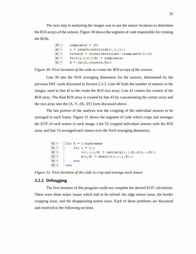
The next step in analyzing the images was to use the sensor locations to determine

the ROI arrays of the sensors. Figure 30 shows the segment of code responsible for creating

the ROIs.

Figure 30: First iteration of the code to create the ROI arrays of the sensors

Line 39 sets the NxN averaging dimension for the sensors, determined by the

previous DSC work discussed in Section 2.3.3. Line 40 finds the number of sensors in the

images, used in line 42 to the create the ROI size array. Line 41 creates the corners of the

ROI array. The final ROI array is created by line 43 by concatenating the corner array and

the size array into the [X, Y, dX, dY] form discussed above.

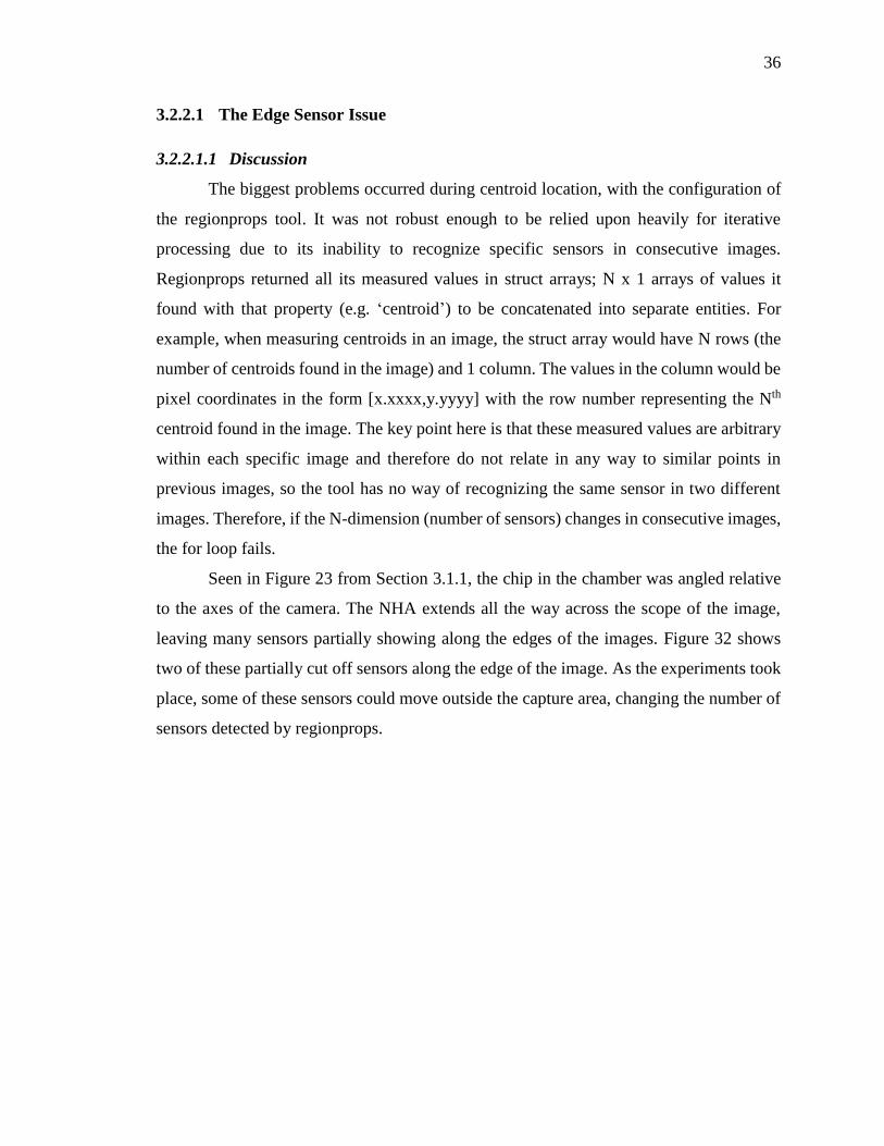
The last portion of the analysis was the cropping of the individual sensors to be

averaged in each frame. Figure 31 shows the segment of code which crops and averages

the EOT of each sensor in each image. Line 52 cropped individual sensors with the ROI

array and line 53 averaged each sensor over the NxN averaging dimension.

Figure 31: First iteration of the code to crop and average each sensor

3.2.2 Debugging

The first iteration of this program could not complete the desired EOT calculation.

There were three major issues which had to be solved: the edge sensor issue, the border

cropping issue, and the disappearing sensor issue. Each of these problems are discussed

and resolved in the following sections.

36

3.2.2.1 The Edge Sensor Issue

3.2.2.1.1 Discussion

The biggest problems occurred during centroid location, with the configuration of

the regionprops tool. It was not robust enough to be relied upon heavily for iterative

processing due to its inability to recognize specific sensors in consecutive images.

Regionprops returned all its measured values in struct arrays; N x 1 arrays of values it

found with that property (e.g. ‘centroid’) to be concatenated into separate entities. For

example, when measuring centroids in an image, the struct array would have N rows (the

number of centroids found in the image) and 1 column. The values in the column would be

pixel coordinates in the form [x.xxxx,y.yyyy] with the row number representing the Nth

centroid found in the image. The key point here is that these measured values are arbitrary

within each specific image and therefore do not relate in any way to similar points in

previous images, so the tool has no way of recognizing the same sensor in two different

images. Therefore, if the N-dimension (number of sensors) changes in consecutive images,

the for loop fails.

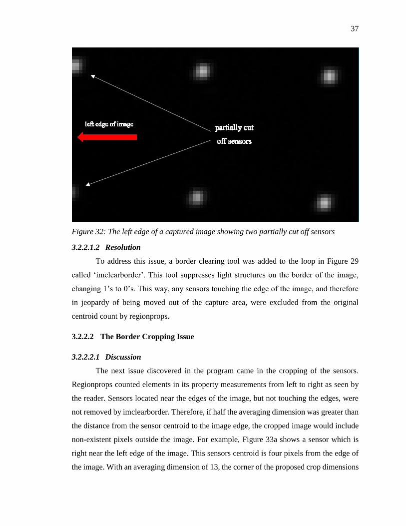
Seen in Figure 23 from Section 3.1.1, the chip in the chamber was angled relative

to the axes of the camera. The NHA extends all the way across the scope of the image,

leaving many sensors partially showing along the edges of the images. Figure 32 shows

two of these partially cut off sensors along the edge of the image. As the experiments took

place, some of these sensors could move outside the capture area, changing the number of

sensors detected by regionprops.

37

Figure 32: The left edge of a captured image showing two partially cut off sensors

3.2.2.1.2 Resolution

To address this issue, a border clearing tool was added to the loop in Figure 29

called ‘imclearborder’. This tool suppresses light structures on the border of the image,

changing 1’s to 0’s. This way, any sensors touching the edge of the image, and therefore

in jeopardy of being moved out of the capture area, were excluded from the original

centroid count by regionprops.

3.2.2.2 The Border Cropping Issue

3.2.2.2.1 Discussion

The next issue discovered in the program came in the cropping of the sensors.

Regionprops counted elements in its property measurements from left to right as seen by

the reader. Sensors located near the edges of the image, but not touching the edges, were

not removed by imclearborder. Therefore, if half the averaging dimension was greater than

the distance from the sensor centroid to the image edge, the cropped image would include

non-existent pixels outside the image. For example, Figure 33a shows a sensor which is

right near the left edge of the image. This sensors centroid is four pixels from the edge of

the image. With an averaging dimension of 13, the corner of the proposed crop dimensions

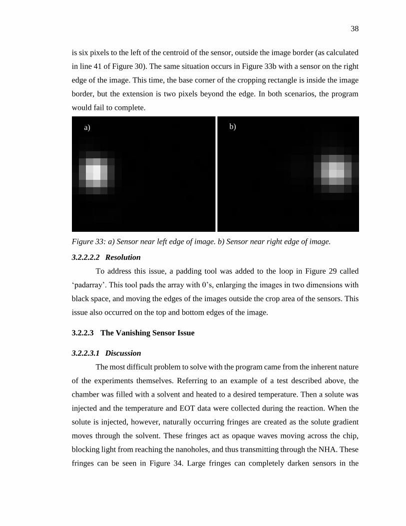
38

is six pixels to the left of the centroid of the sensor, outside the image border (as calculated

in line 41 of Figure 30). The same situation occurs in Figure 33b with a sensor on the right

edge of the image. This time, the base corner of the cropping rectangle is inside the image

border, but the extension is two pixels beyond the edge. In both scenarios, the program

would fail to complete.

Figure 33: a) Sensor near left edge of image. b) Sensor near right edge of image.

3.2.2.2.2 Resolution

To address this issue, a padding tool was added to the loop in Figure 29 called

‘padarray’. This tool pads the array with 0’s, enlarging the images in two dimensions with

black space, and moving the edges of the images outside the crop area of the sensors. This

issue also occurred on the top and bottom edges of the image.

3.2.2.3 The Vanishing Sensor Issue

3.2.2.3.1 Discussion

The most difficult problem to solve with the program came from the inherent nature

of the experiments themselves. Referring to an example of a test described above, the

chamber was filled with a solvent and heated to a desired temperature. Then a solute was

injected and the temperature and EOT data were collected during the reaction. When the

solute is injected, however, naturally occurring fringes are created as the solute gradient

moves through the solvent. These fringes act as opaque waves moving across the chip,

blocking light from reaching the nanoholes, and thus transmitting through the NHA. These

fringes can be seen in Figure 34. Large fringes can completely darken sensors in the

a) b)

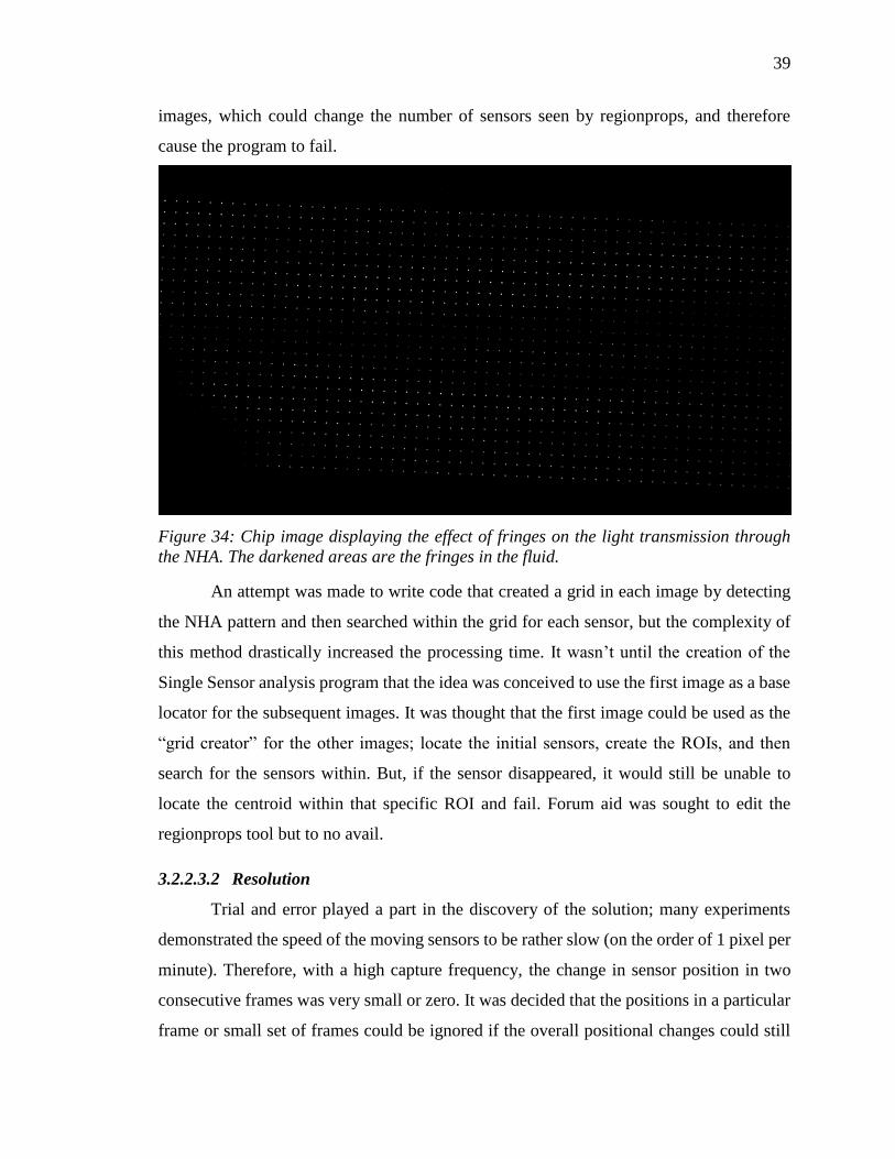
39

images, which could change the number of sensors seen by regionprops, and therefore

cause the program to fail.

Figure 34: Chip image displaying the effect of fringes on the light transmission through

the NHA. The darkened areas are the fringes in the fluid.

An attempt was made to write code that created a grid in each image by detecting

the NHA pattern and then searched within the grid for each sensor, but the complexity of

this method drastically increased the processing time. It wasn’t until the creation of the

Single Sensor analysis program that the idea was conceived to use the first image as a base

locator for the subsequent images. It was thought that the first image could be used as the

“grid creator” for the other images; locate the initial sensors, create the ROIs, and then

search for the sensors within. But, if the sensor disappeared, it would still be unable to

locate the centroid within that specific ROI and fail. Forum aid was sought to edit the

regionprops tool but to no avail.

3.2.2.3.2 Resolution

Trial and error played a part in the discovery of the solution; many experiments

demonstrated the speed of the moving sensors to be rather slow (on the order of 1 pixel per

minute). Therefore, with a high capture frequency, the change in sensor position in two

consecutive frames was very small or zero. It was decided that the positions in a particular

frame or small set of frames could be ignored if the overall positional changes could still

40

be accurately tracked. This lead to the best solution to the disappearing sensors issue: a

comparison of the original number of sensors to the number found in each subsequent

image.

The bwlabel tool was used in the for loop to count the number of centroids found

in each image and compare that number to the number of centroids found in the first image.

The rationale was that the first image, unaffected by the turmoil of the experiment, could

be used as a baseline for the ‘correct’ number of sensors to look for in each subsequent

image. Then a simple if statement was used to check for the correct sensor number, and if

not, the previous sensor locations could be used instead. Once again, this was possible due

to the very small changes in sensor location between consecutive images.

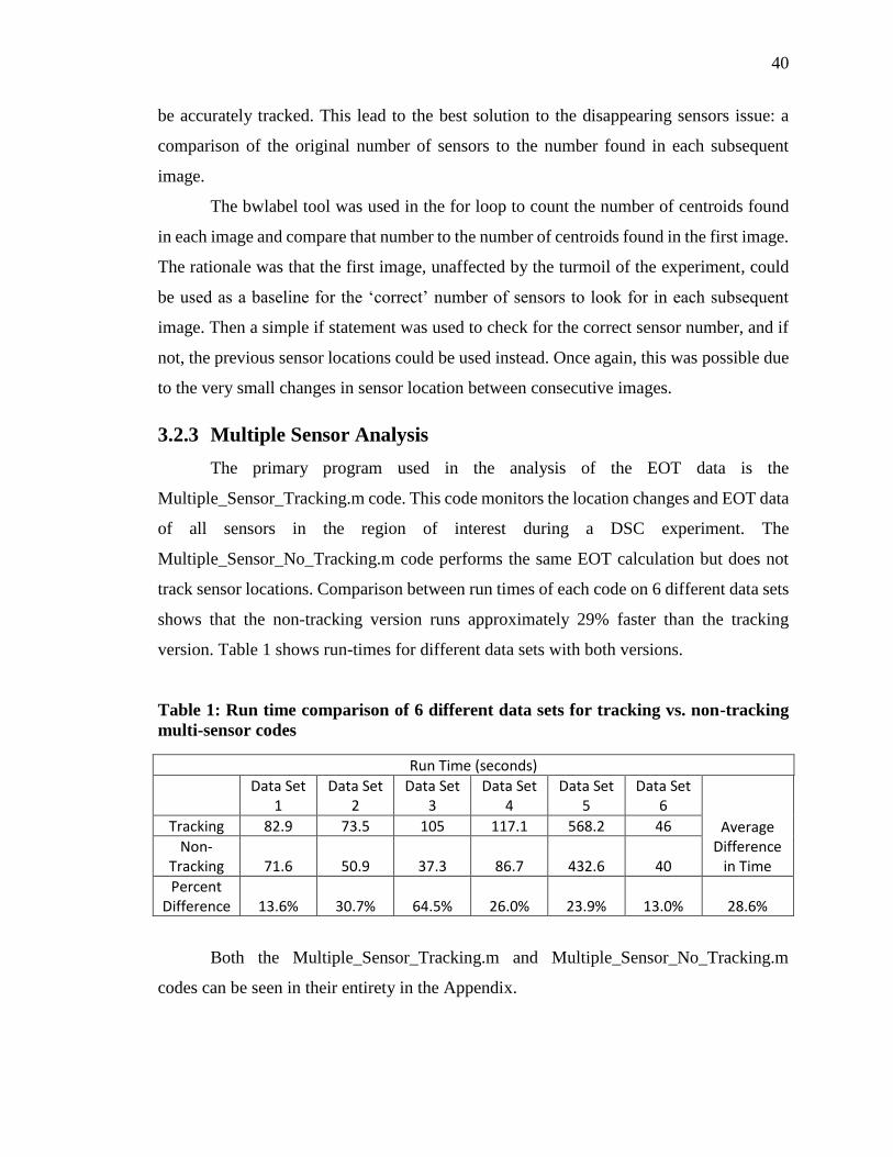
3.2.3 Multiple Sensor Analysis

The primary program used in the analysis of the EOT data is the

Multiple_Sensor_Tracking.m code. This code monitors the location changes and EOT data

of all sensors in the region of interest during a DSC experiment. The

Multiple_Sensor_No_Tracking.m code performs the same EOT calculation but does not

track sensor locations. Comparison between run times of each code on 6 different data sets

shows that the non-tracking version runs approximately 29% faster than the tracking

version. Table 1 shows run-times for different data sets with both versions.

Table 1: Run time comparison of 6 different data sets for tracking vs. non-tracking

multi-sensor codes

Run Time (seconds)

Data Set

1 Data Set

2 Data Set

3 Data Set

4 Data Set

5 Data Set

6

Average Difference

in Time

Tracking 82.9 73.5 105 117.1 568.2 46

Non-Tracking 71.6 50.9 37.3 86.7 432.6 40

Percent Difference 13.6% 30.7% 64.5% 26.0% 23.9% 13.0% 28.6%

Both the Multiple_Sensor_Tracking.m and Multiple_Sensor_No_Tracking.m

codes can be seen in their entirety in the Appendix.

41

3.2.3.1 Procedure

Using either of the multiple sensor analysis programs to calculate EOT was

straightforward if the capture program procedures outlined in Section 3.1 were followed

correctly. When the experiment had ended and the data had been collected, it was loaded

onto an external drive and transferred over to the post-processing computer. The data

(images and temperature data) was contained in its own folder entitled with the experiment

date and details for clarity. For example, a folder for an experiment conducted on 8/17/17

where 40 μL of ethanol was injected into 80 μL of water at a rate of 40 μL/min through the

top port was named “081717_40eth_40_80h2o_top.” Any other details of the experiment

were also documented separately.

When the data was loaded onto the post-processing computer, the post-processing

program was opened. The program was created to analyze the images in the “current

folder,” so the test to be analyzed was opened in the directory (referring to the above

example, the directory read C:\...\081717_40eth_40_80h2o_top).

The next step was to determine the size each image was to be cropped to. Referring

to Line 16 in Figure 28, the ‘rect’ variable was adjusted based on which area of sensors

was to be analyzed. To find the dimensions of the crop, another image processing tool

called “impixelinfo” was used in the command window. This shows the pixel coordinates

of the mouse while it is over a displayed image (shown by first entering

“imshow(‘ImageX’)” into the command window). This tool allowed the user to find the

desired dimensions of the area they wished to analyze and set ‘rect’ in the same form [X Y

dX dY] referenced in Section 3.1.2.1 above.

The final step was to reference the accompanying temperature data from the

experiment (if there is any) for plotting. Below the meat of the program were plotting

sections which were previously used. For an excel file, the “xlsread” tool was very useful.

For more information on this, type “help xlsread” into the command window in MATLAB.

3.2.4 Single Sensor Analysis

One of the benefits of the Field Capture Method was the ability to capture data at

much greater frequencies than the Sensor Location Method. As the image capture area

decreased, the capture rate increased. The Region of Interest Control Edition brought about

42

tests which looked at a single sensor’s EOT during a sudden temperature change. The

objective was to display the sensitivity and response time of the EOT of a nanohole. These

results and the results of the tests to determine the maximum capture rates are presented

and discussed in Sections 4.3 and 4.4

The Single_Sensor_Tracking.m was the main post-processing program used in the

analysis. It had the ability to track sensors if desired by the user, but it was often

unnecessary because the experiments were not long enough to see noticeable location

changes.

Both the Single_Sensor_Tracking.m and Single_Sensor_No_Tracking.m programs

can be seen in their entirety in the Appendix.

3.2.4.1 Procedure

The procedure for either of the single sensor programs was the same as the multiple

sensor programs’. The only difference was that the program did not require a ‘rect’ variable

to crop the images because the images only looked at a single sensor.

Accompanying temperature data was also referenced in the same way as the

multiple sensor programs’.

4 TESTS AND RESULTS

This section presents and discusses the results of the experiments conducted with

the programs detailed in Section 3.

4.1 COMPARISON TO SENSOR LOCATION METHOD

The first test to determine the validity of the Full Field Image Capture Method was

the comparison to the Sensor Location Method used in the laboratory. Multiple documents

published by the laboratory [4, 3, 5, 7, 6] have confirmed the Sensor Location Method’s

ability to produce an accurate temperature sensor from EOT through an NHA chip. To

compare the methods, the following Comparison Injection Test was designed:

Run two identical tests; first with the Sensor Location Method, then with the Full

Field Image Capture Method, and compare the change in EOT of the sensors in each test.

43

Ideally, identical tests should have identical EOT change. Experimentally, identical tests

should show similar EOT change, specifically the shapes of the EOT profile in time.

The chamber assembly was filled with 90 μL of water and 30 μL of ethanol was

injected at 30 μL/min while the reaction was observed. With the post-processing programs,

the EOT changes were compared for both individually selected sensors and all sensors

averaged together. Section 4.1.1 provides a detailed general procedure of the Comparison

Injection Tests.

4.1.1 General Procedure for Comparison Injection Test

In the Comparison Injection Tests discussed in Section 4.1, the detailed procedure

used was as follows:

1. The Chamber Flow Cell, as seen in Figure 16, was assembled and mounted to

the rotational XYZ stage.

2. The chamber was filled with the solvent: 90 μL of DI water.

3. The LED light and CCD camera were turned on.

4. The Calibration Program was opened and used to focus the CCD camera onto

the NHA.

5. The LFI-3751 temperature controller was turned on.

6. The LFI-3751 temperature controller VI was opened and used to heat the

chamber to the desired temperature (approx. 40°C in this case).

7. The solute, ethanol at room temperature, was loaded into a syringe and set up

in the syringe pump.

8. The syringe pump was programmed to expel a volume of 30 μL at a rate of 30

μL/min.

9. The Sensor Location Method’s VI was run and the injection was initiated. Data

was captured and moved to the post-processing computer.

10. The LFI, LED, and CCD camera were shut down.

11. The chamber was emptied and flushed twice; first with DI water, second with

air.

12. Steps 2 through 8 were repeated.

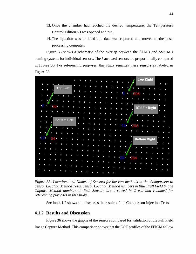
44

13. Once the chamber had reached the desired temperature, the Temperature

Control Edition VI was opened and run.

14. The injection was initiated and data was captured and moved to the post-

processing computer.

Figure 35 shows a schematic of the overlap between the SLM’s and SSICM’s

naming systems for individual sensors. The 5 arrowed sensors are proportionally compared

in Figure 36. For referencing purposes, this study renames these sensors as labeled in

Figure 35.

Figure 35: Locations and Names of Sensors for the two methods in the Comparison to

Sensor Location Method Tests. Sensor Location Method numbers in Blue, Full Field Image

Capture Method numbers in Red. Sensors are arrowed in Green and renamed for

referencing purposes in this study.

Section 4.1.2 shows and discusses the results of the Comparison Injection Tests.

4.1.2 Results and Discussion

Figure 36 shows the graphs of the sensors compared for validation of the Full Field

Image Capture Method. This comparison shows that the EOT profiles of the FFICM follow

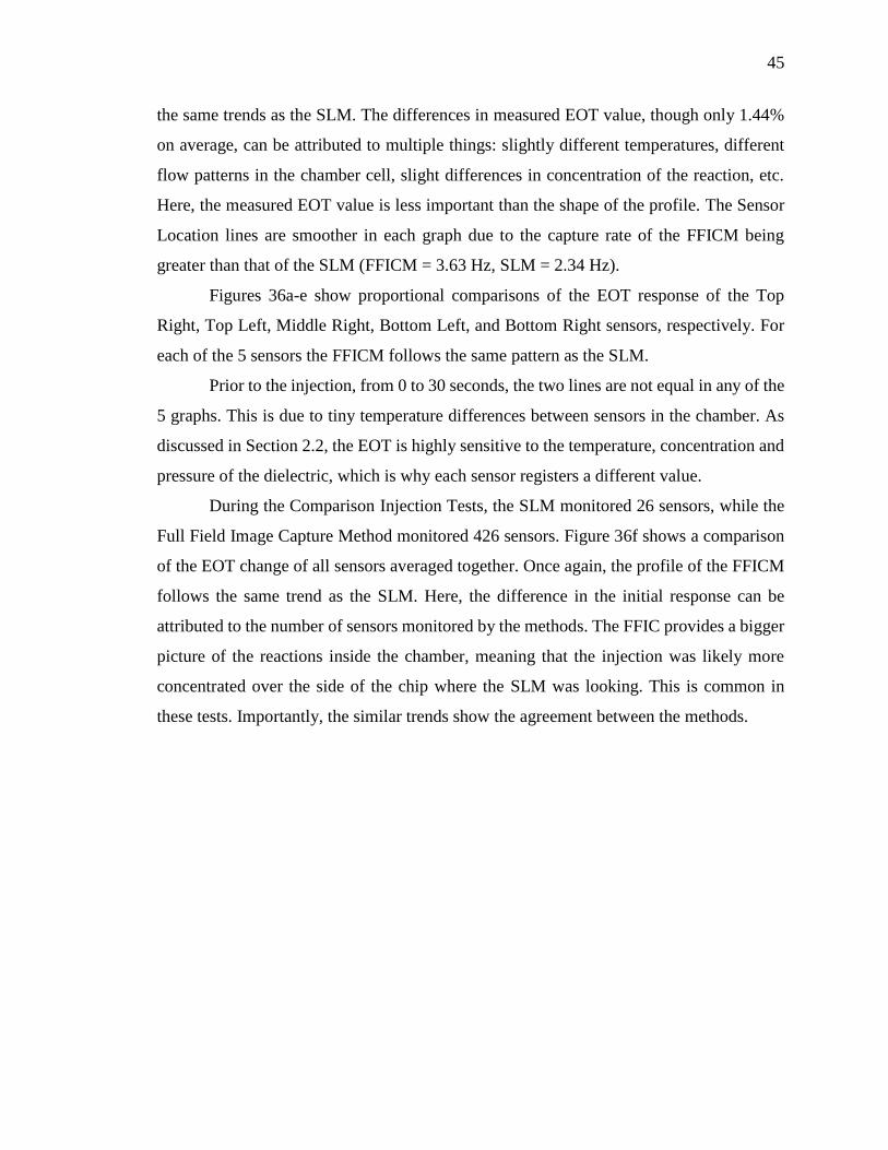
45

the same trends as the SLM. The differences in measured EOT value, though only 1.44%

on average, can be attributed to multiple things: slightly different temperatures, different

flow patterns in the chamber cell, slight differences in concentration of the reaction, etc.

Here, the measured EOT value is less important than the shape of the profile. The Sensor

Location lines are smoother in each graph due to the capture rate of the FFICM being

greater than that of the SLM (FFICM = 3.63 Hz, SLM = 2.34 Hz).

Figures 36a-e show proportional comparisons of the EOT response of the Top

Right, Top Left, Middle Right, Bottom Left, and Bottom Right sensors, respectively. For

each of the 5 sensors the FFICM follows the same pattern as the SLM.

Prior to the injection, from 0 to 30 seconds, the two lines are not equal in any of the

5 graphs. This is due to tiny temperature differences between sensors in the chamber. As

discussed in Section 2.2, the EOT is highly sensitive to the temperature, concentration and

pressure of the dielectric, which is why each sensor registers a different value.

During the Comparison Injection Tests, the SLM monitored 26 sensors, while the

Full Field Image Capture Method monitored 426 sensors. Figure 36f shows a comparison

of the EOT change of all sensors averaged together. Once again, the profile of the FFICM

follows the same trend as the SLM. Here, the difference in the initial response can be

attributed to the number of sensors monitored by the methods. The FFIC provides a bigger

picture of the reactions inside the chamber, meaning that the injection was likely more

concentrated over the side of the chip where the SLM was looking. This is common in

these tests. Importantly, the similar trends show the agreement between the methods.

46

Figure 36: Proportional Comparisons of the Sensor Location Method vs. the Full Field

Image Capture Method; a) Top Right; b) Top Left; c) Middle Right; d) Bottom Left; e)

Bottom Right; f) All Sensors Averaged

a)

b)

c)

d)

e)

f)

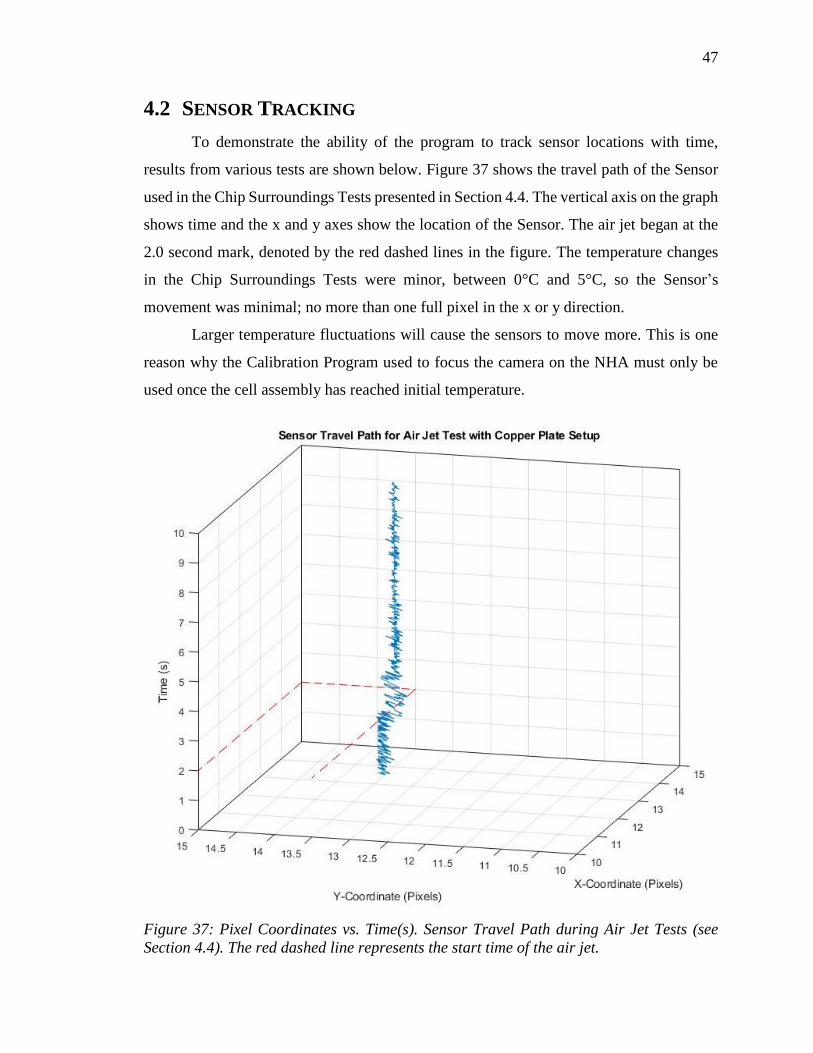
47

4.2 SENSOR TRACKING

To demonstrate the ability of the program to track sensor locations with time,

results from various tests are shown below. Figure 37 shows the travel path of the Sensor

used in the Chip Surroundings Tests presented in Section 4.4. The vertical axis on the graph

shows time and the x and y axes show the location of the Sensor. The air jet began at the

2.0 second mark, denoted by the red dashed lines in the figure. The temperature changes

in the Chip Surroundings Tests were minor, between 0°C and 5°C, so the Sensor’s

movement was minimal; no more than one full pixel in the x or y direction.

Larger temperature fluctuations will cause the sensors to move more. This is one

reason why the Calibration Program used to focus the camera on the NHA must only be

used once the cell assembly has reached initial temperature.

Figure 37: Pixel Coordinates vs. Time(s). Sensor Travel Path during Air Jet Tests (see

Section 4.4). The red dashed line represents the start time of the air jet.

48

During heating prior to one experiment in the Chip Surroundings Tests, a

temperature change of 16.3°C, from room temperature of 26.3°C to initial temperature of

42.6°C, caused the targeted Sensor to move from pixel location (315,1314) to (339, 1338).

24 pixels in the x-direction and 24 pixels in the y-direction produces a total lateral

movement of 33.94 pixels, or 25.12 μm (see Section 2.3.3). This is slightly less than the

lattice constant between sensors. Considering the relative size of one sensor, this is a very

large difference. This is another experiment that validates the necessity of the technology

developed in this study for the laboratory to move into Differential Scanning Calorimetry.

4.3 CAPTURE SPEED TESTS

To demonstrate the maximum capture speed of the Field Capture Programs, the

Region-of-Interest Control Edition was tested for a range of image sizes. The sizes were

chosen based on commonly used image sizes in the laboratory. Table 2 shows the image

dimensions and describes the use of each size by the laboratory. Referring to Section 3.1.2,

the dimensions of each image in the ROI Control Edition are specified in [Xinitial Yinitial

Xwidth Yheight] form where Xinitial and Yinitial are measured from the top left corner of the

image.

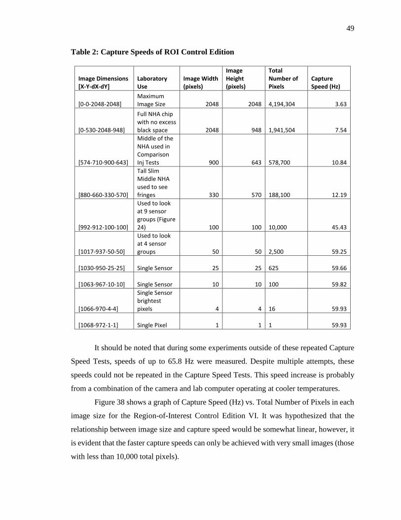
49

Table 2: Capture Speeds of ROI Control Edition

Image Dimensions [X-Y-dX-dY]

Laboratory Use

Image Width (pixels)

Image Height (pixels)

Total Number of Pixels

Capture Speed (Hz)

[0-0-2048-2048] Maximum Image Size 2048 2048

4,194,304 3.63

[0-530-2048-948]

Full NHA chip with no excess black space 2048 948

1,941,504 7.54

[574-710-900-643]

Middle of the NHA used in Comparison Inj Tests 900 643

578,700 10.84

[880-660-330-570]

Tall Slim Middle NHA used to see fringes 330 570

188,100 12.19

[992-912-100-100]

Used to look at 9 sensor groups (Figure 24) 100 100

10,000 45.43

[1017-937-50-50]

Used to look at 4 sensor groups 50 50

2,500 59.25

[1030-950-25-25] Single Sensor 25 25 625 59.66

[1063-967-10-10] Single Sensor 10 10 100 59.82

[1066-970-4-4]

Single Sensor brightest pixels 4 4

16 59.93

[1068-972-1-1] Single Pixel 1 1 1 59.93

It should be noted that during some experiments outside of these repeated Capture

Speed Tests, speeds of up to 65.8 Hz were measured. Despite multiple attempts, these

speeds could not be repeated in the Capture Speed Tests. This speed increase is probably

from a combination of the camera and lab computer operating at cooler temperatures.

Figure 38 shows a graph of Capture Speed (Hz) vs. Total Number of Pixels in each

image size for the Region-of-Interest Control Edition VI. It was hypothesized that the

relationship between image size and capture speed would be somewhat linear, however, it

is evident that the faster capture speeds can only be achieved with very small images (those

with less than 10,000 total pixels).

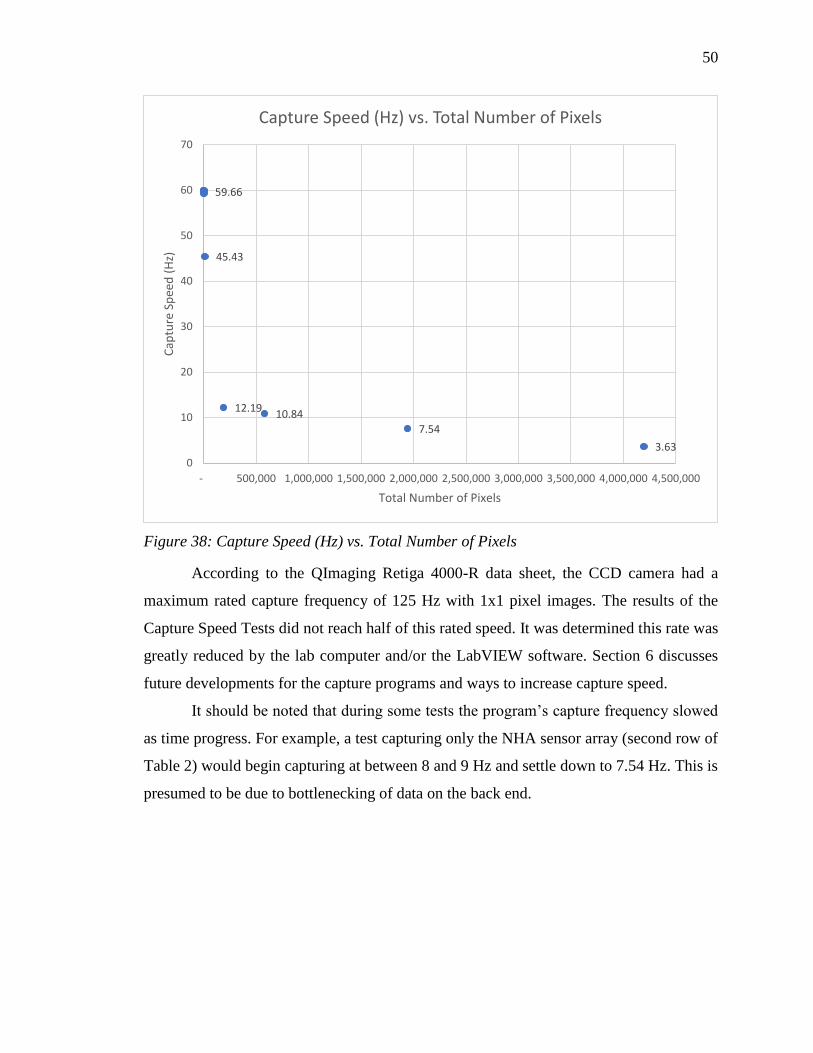
50

Figure 38: Capture Speed (Hz) vs. Total Number of Pixels

According to the QImaging Retiga 4000-R data sheet, the CCD camera had a

maximum rated capture frequency of 125 Hz with 1x1 pixel images. The results of the

Capture Speed Tests did not reach half of this rated speed. It was determined this rate was

greatly reduced by the lab computer and/or the LabVIEW software. Section 6 discusses

future developments for the capture programs and ways to increase capture speed.

It should be noted that during some tests the program’s capture frequency slowed

as time progress. For example, a test capturing only the NHA sensor array (second row of

Table 2) would begin capturing at between 8 and 9 Hz and settle down to 7.54 Hz. This is

presumed to be due to bottlenecking of data on the back end.

3.63

7.54

10.8412.19

45.43

59.66

0

10

20

30

40

50

60

70

- 500,000 1,000,000 1,500,000 2,000,000 2,500,000 3,000,000 3,500,000 4,000,000 4,500,000

Cap

ture

Sp

eed

(H

z)

Total Number of Pixels

Capture Speed (Hz) vs. Total Number of Pixels

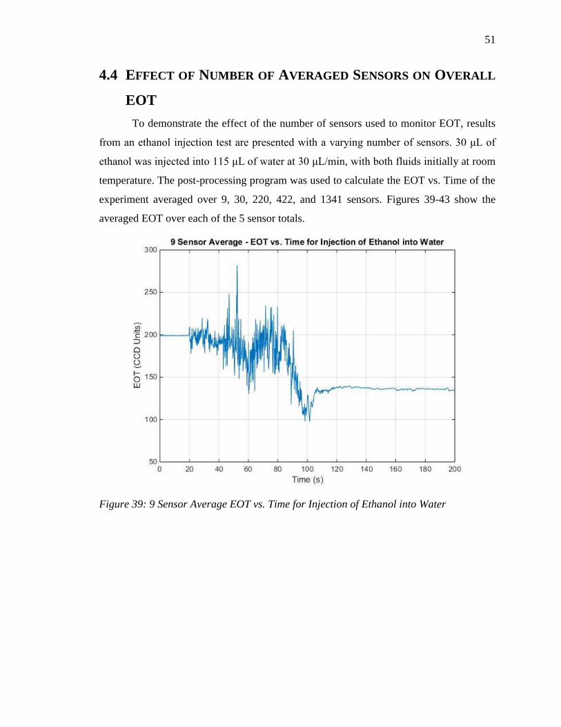
51

4.4 EFFECT OF NUMBER OF AVERAGED SENSORS ON OVERALL

EOT

To demonstrate the effect of the number of sensors used to monitor EOT, results

from an ethanol injection test are presented with a varying number of sensors. 30 μL of

ethanol was injected into 115 μL of water at 30 μL/min, with both fluids initially at room

temperature. The post-processing program was used to calculate the EOT vs. Time of the

experiment averaged over 9, 30, 220, 422, and 1341 sensors. Figures 39-43 show the

averaged EOT over each of the 5 sensor totals.

Figure 39: 9 Sensor Average EOT vs. Time for Injection of Ethanol into Water

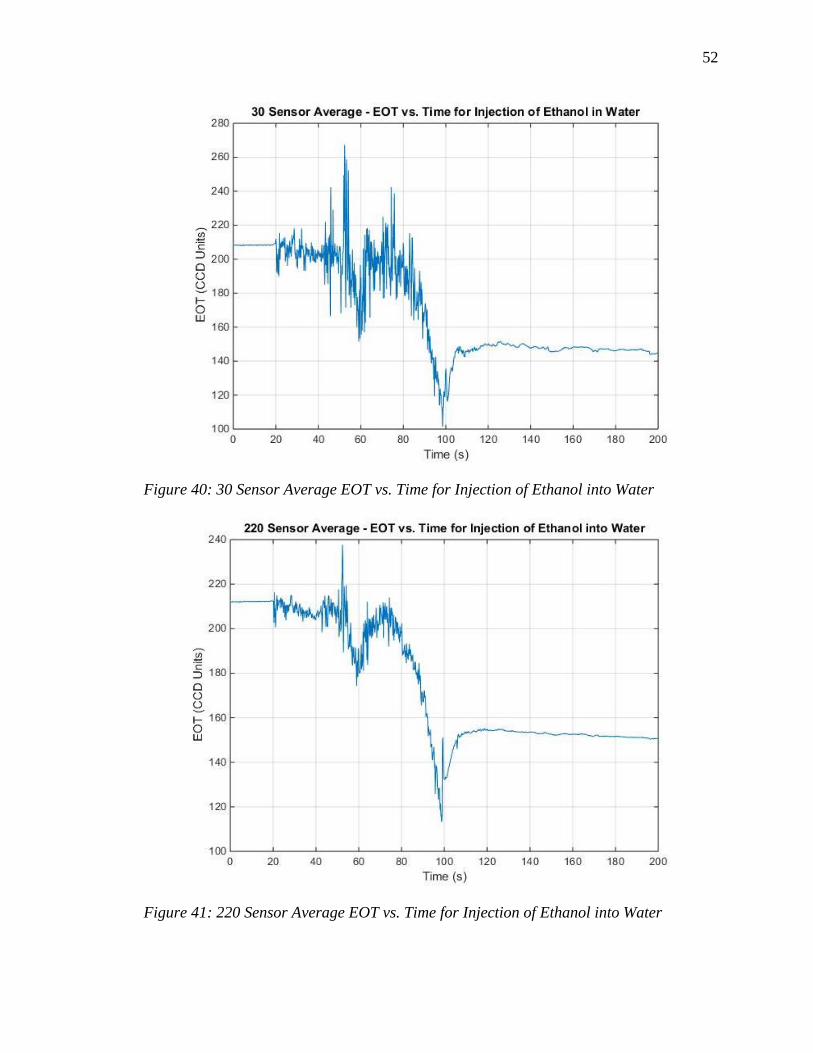
52

Figure 40: 30 Sensor Average EOT vs. Time for Injection of Ethanol into Water

Figure 41: 220 Sensor Average EOT vs. Time for Injection of Ethanol into Water

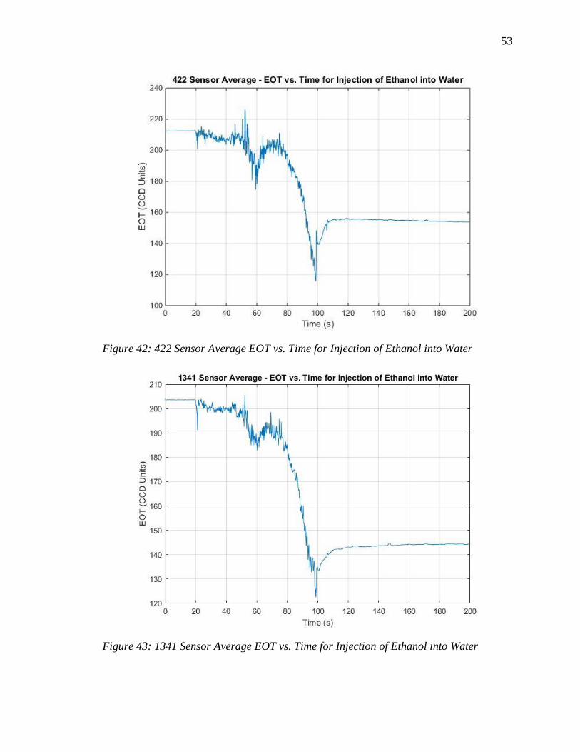
53

Figure 42: 422 Sensor Average EOT vs. Time for Injection of Ethanol into Water

Figure 43: 1341 Sensor Average EOT vs. Time for Injection of Ethanol into Water

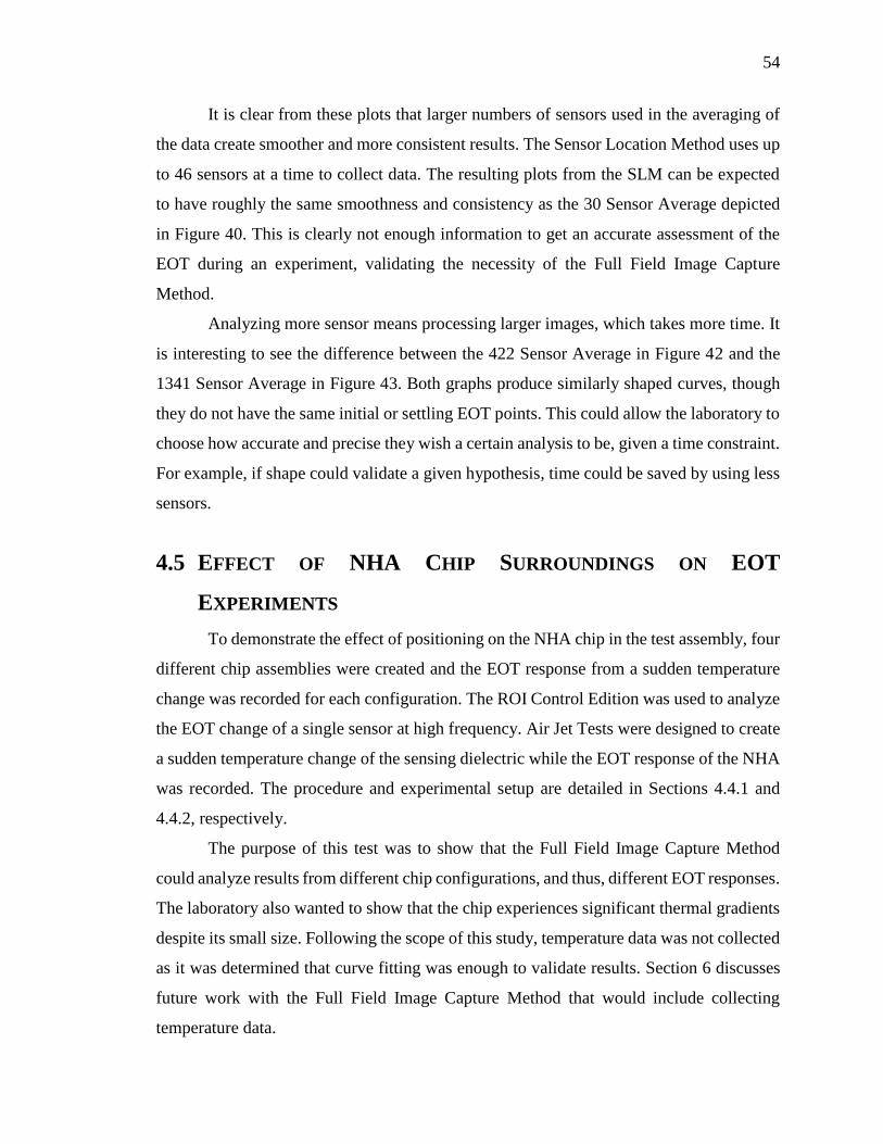
54

It is clear from these plots that larger numbers of sensors used in the averaging of

the data create smoother and more consistent results. The Sensor Location Method uses up

to 46 sensors at a time to collect data. The resulting plots from the SLM can be expected

to have roughly the same smoothness and consistency as the 30 Sensor Average depicted

in Figure 40. This is clearly not enough information to get an accurate assessment of the

EOT during an experiment, validating the necessity of the Full Field Image Capture

Method.

Analyzing more sensor means processing larger images, which takes more time. It

is interesting to see the difference between the 422 Sensor Average in Figure 42 and the

1341 Sensor Average in Figure 43. Both graphs produce similarly shaped curves, though

they do not have the same initial or settling EOT points. This could allow the laboratory to

choose how accurate and precise they wish a certain analysis to be, given a time constraint.

For example, if shape could validate a given hypothesis, time could be saved by using less

sensors.

4.5 EFFECT OF NHA CHIP SURROUNDINGS ON EOT

EXPERIMENTS

To demonstrate the effect of positioning on the NHA chip in the test assembly, four

different chip assemblies were created and the EOT response from a sudden temperature

change was recorded for each configuration. The ROI Control Edition was used to analyze

the EOT change of a single sensor at high frequency. Air Jet Tests were designed to create

a sudden temperature change of the sensing dielectric while the EOT response of the NHA

was recorded. The procedure and experimental setup are detailed in Sections 4.4.1 and

4.4.2, respectively.

The purpose of this test was to show that the Full Field Image Capture Method

could analyze results from different chip configurations, and thus, different EOT responses.

The laboratory also wanted to show that the chip experiences significant thermal gradients

despite its small size. Following the scope of this study, temperature data was not collected

as it was determined that curve fitting was enough to validate results. Section 6 discusses

future work with the Full Field Image Capture Method that would include collecting

temperature data.

55

4.5.1 Procedure

To demonstrate the effect of positioning on the NHA chip in different assemblies,

a test was designed to monitor the EOT change from a sudden temperature change of the

sensing dielectric. A single sensor was observed to maximize the capture frequency of the

ROI Control Edition. This experiment was conducted without the use of the chamber

discussed in Section 2.3.1. This made the sudden temperature change easy to create with a

Dust-Off Compressed Air Duster. The following steps were followed during each test:

1. One of the four configurations discussed in Section 4.4.2 was assembled onto

the rotational XYZ stage.

2. The thermistor accompanying the assembly was positioned to read the

temperature of the heater.

3. The heater was connected to the power supply and the voltage and current were

adjusted to raise the temperature of the of the heater to roughly 40°C (this was

typically at about V = 1.0 V and I = 0.5 A).

4. The Calibration Program was opened and the CCD camera was focused onto

the NHA with the rotational XYZ stage.

5. The ROI Control Edition was opened and the sensor of interest was identified

and targeted. 25 x 25 pixel images were captured for all tests.

6. Simultaneously, the program and a separate timer were started with each hand.

7. The duster’s straw tip was held approximately 4.0 mm from the chip face and

slightly to one side to not block the light from passing through the NHA. Again,

simultaneously, the duster’s trigger was pushed and the ‘lap’ was clicked on the

timer to mark the beginning of the air jet. The jet lasted approximately 1 second.

8. Steps 6 and 7 were performed very quickly to limit the number of excess images

captured by the program.

9. The program was stopped and the data was transferred to the post-processing

computer for analysis.

Due the nature of the procedure (specifically Step 7), human error must be factored

into the certainty of the reported start and stop times of the jet on the results graphs below.

It was very difficult to accurately mark the time and begin the jet simultaneously.

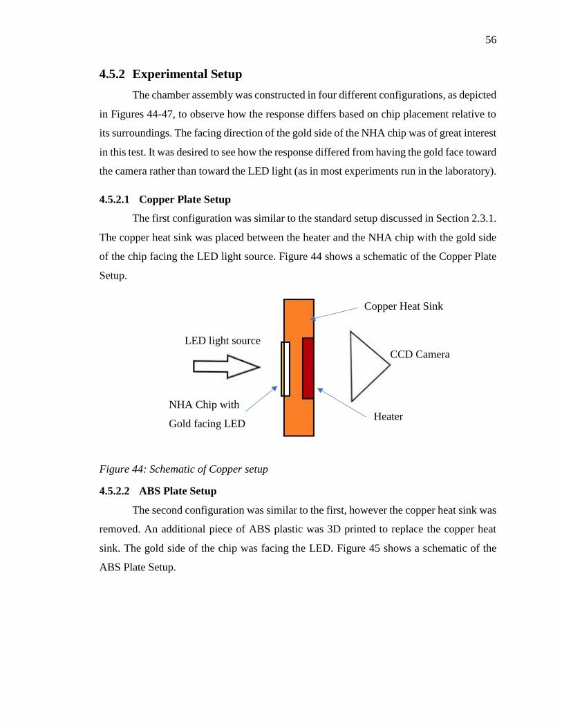
56

4.5.2 Experimental Setup

The chamber assembly was constructed in four different configurations, as depicted

in Figures 44-47, to observe how the response differs based on chip placement relative to

its surroundings. The facing direction of the gold side of the NHA chip was of great interest

in this test. It was desired to see how the response differed from having the gold face toward

the camera rather than toward the LED light (as in most experiments run in the laboratory).

4.5.2.1 Copper Plate Setup

The first configuration was similar to the standard setup discussed in Section 2.3.1.

The copper heat sink was placed between the heater and the NHA chip with the gold side

of the chip facing the LED light source. Figure 44 shows a schematic of the Copper Plate

Setup.

Figure 44: Schematic of Copper setup

4.5.2.2 ABS Plate Setup

The second configuration was similar to the first, however the copper heat sink was

removed. An additional piece of ABS plastic was 3D printed to replace the copper heat

sink. The gold side of the chip was facing the LED. Figure 45 shows a schematic of the

ABS Plate Setup.

LED light source

Copper Heat Sink

CCD Camera

Heater NHA Chip with

Gold facing LED

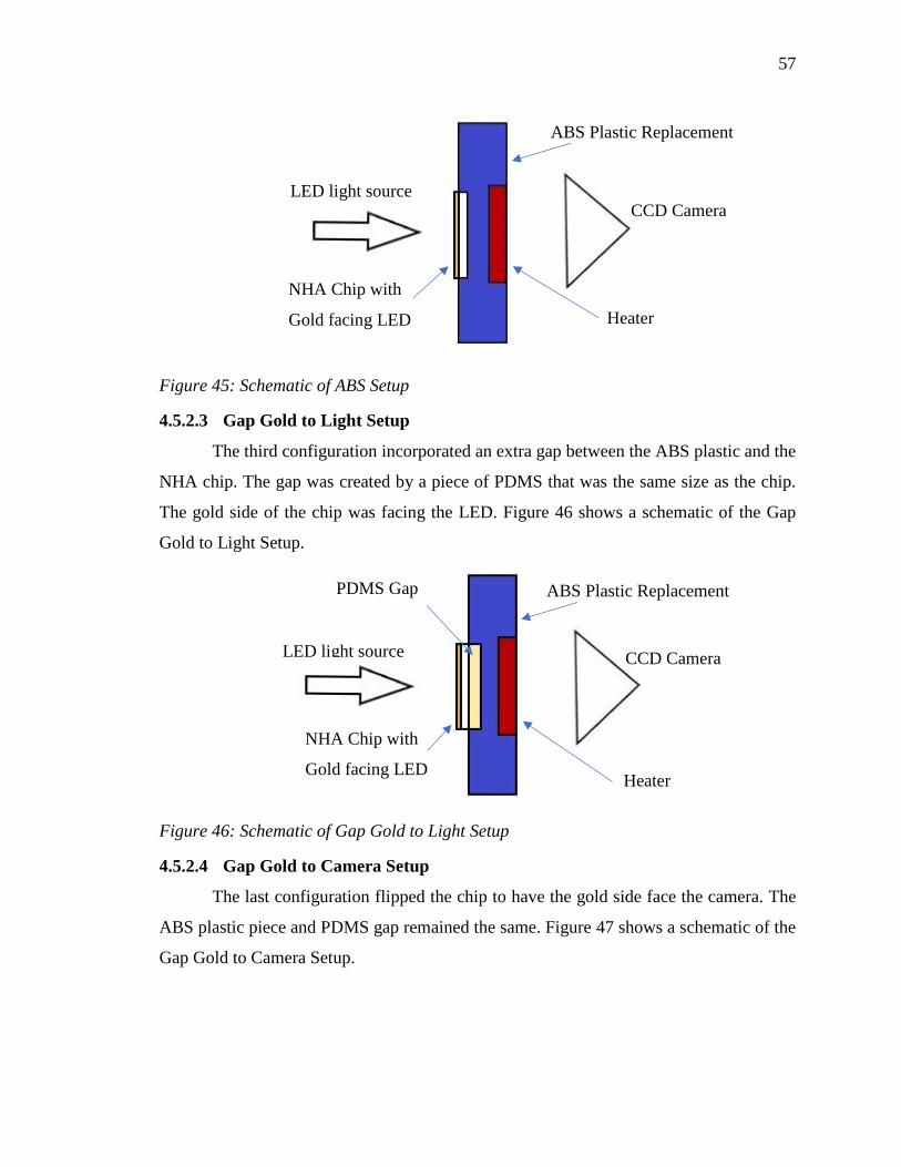
57

Figure 45: Schematic of ABS Setup

4.5.2.3 Gap Gold to Light Setup

The third configuration incorporated an extra gap between the ABS plastic and the

NHA chip. The gap was created by a piece of PDMS that was the same size as the chip.

The gold side of the chip was facing the LED. Figure 46 shows a schematic of the Gap

Gold to Light Setup.

Figure 46: Schematic of Gap Gold to Light Setup

4.5.2.4 Gap Gold to Camera Setup

The last configuration flipped the chip to have the gold side face the camera. The

ABS plastic piece and PDMS gap remained the same. Figure 47 shows a schematic of the

Gap Gold to Camera Setup.

LED light source

ABS Plastic Replacement

CCD Camera

Heater

NHA Chip with

Gold facing LED

PDMS Gap

Heater

CCD Camera

ABS Plastic Replacement

NHA Chip with

Gold facing LED

LED light source

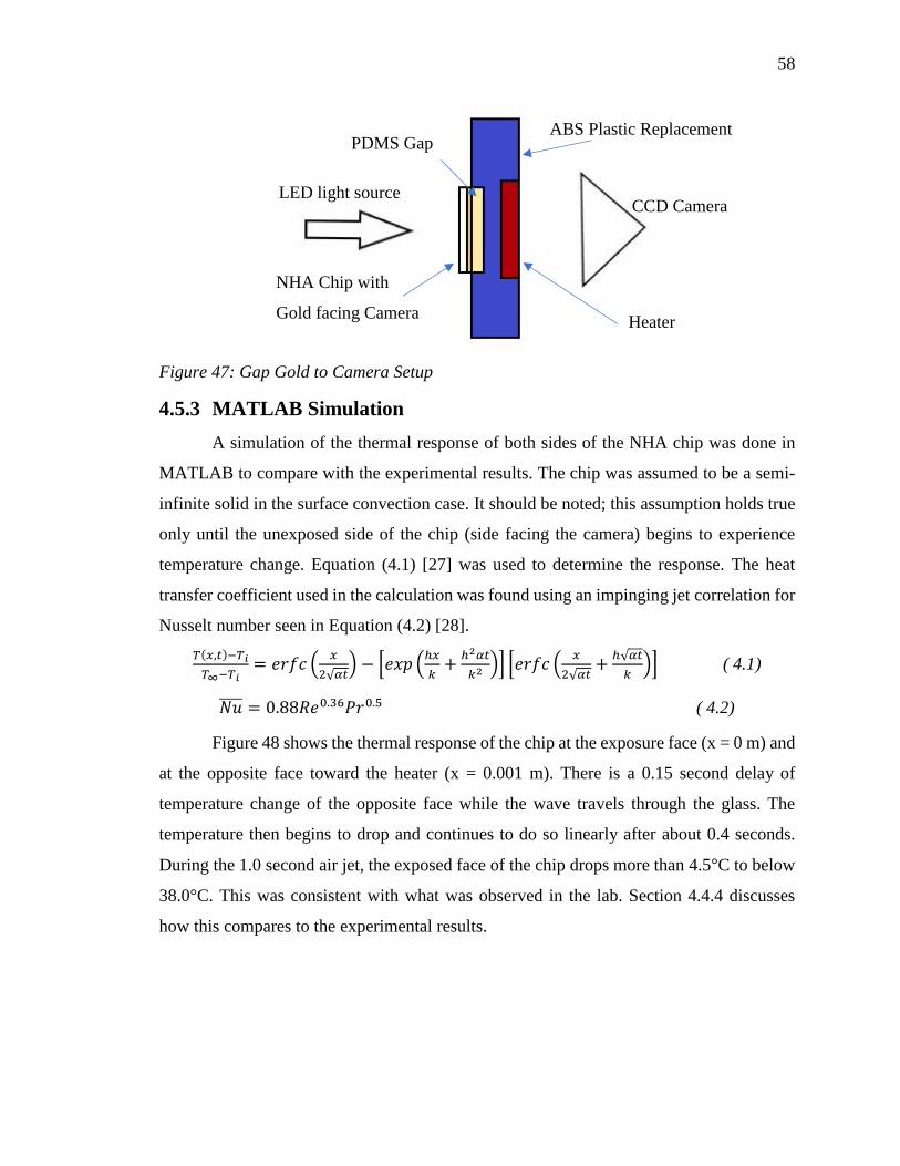
58

Figure 47: Gap Gold to Camera Setup

4.5.3 MATLAB Simulation

A simulation of the thermal response of both sides of the NHA chip was done in

MATLAB to compare with the experimental results. The chip was assumed to be a semi-

infinite solid in the surface convection case. It should be noted; this assumption holds true

only until the unexposed side of the chip (side facing the camera) begins to experience

temperature change. Equation (4.1) [27] was used to determine the response. The heat

transfer coefficient used in the calculation was found using an impinging jet correlation for

Nusselt number seen in Equation (4.2) [28].

𝑇(𝑥,𝑡)−𝑇𝑖

𝑇∞−𝑇𝑖= 𝑒𝑟𝑓𝑐 (

𝑥

2√𝛼𝑡) − [𝑒𝑥𝑝 (

ℎ𝑥

𝑘+

ℎ2𝛼𝑡

𝑘2 )] [𝑒𝑟𝑓𝑐 (𝑥

2√𝛼𝑡+

ℎ√𝛼𝑡

𝑘)] ( 4.1)

𝑁𝑢̅̅ ̅̅ = 0.88𝑅𝑒0.36𝑃𝑟0.5 ( 4.2)

Figure 48 shows the thermal response of the chip at the exposure face (x = 0 m) and

at the opposite face toward the heater (x = 0.001 m). There is a 0.15 second delay of

temperature change of the opposite face while the wave travels through the glass. The

temperature then begins to drop and continues to do so linearly after about 0.4 seconds.

During the 1.0 second air jet, the exposed face of the chip drops more than 4.5°C to below

38.0°C. This was consistent with what was observed in the lab. Section 4.4.4 discusses

how this compares to the experimental results.

Heater

CCD Camera

ABS Plastic Replacement PDMS Gap

LED light source

NHA Chip with

Gold facing Camera

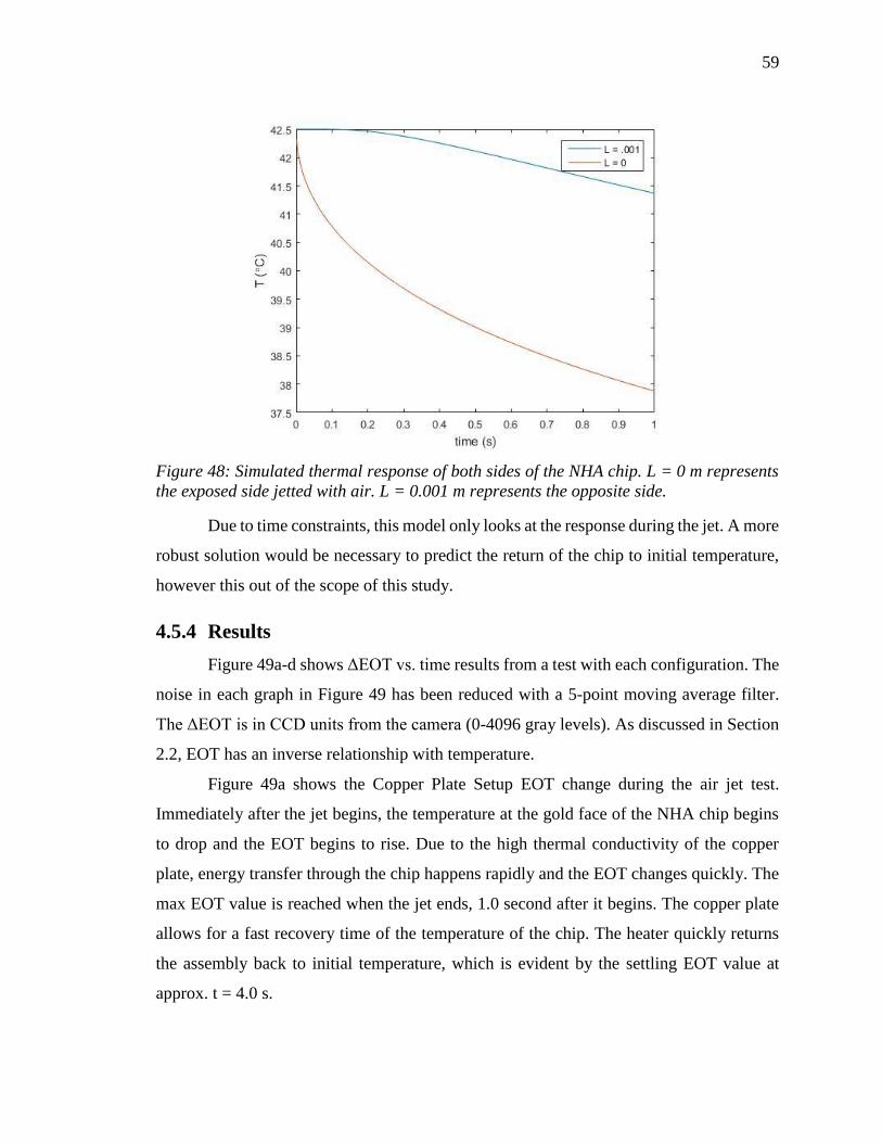
59

Figure 48: Simulated thermal response of both sides of the NHA chip. L = 0 m represents

the exposed side jetted with air. L = 0.001 m represents the opposite side.

Due to time constraints, this model only looks at the response during the jet. A more

robust solution would be necessary to predict the return of the chip to initial temperature,

however this out of the scope of this study.

4.5.4 Results

Figure 49a-d shows ΔEOT vs. time results from a test with each configuration. The

noise in each graph in Figure 49 has been reduced with a 5-point moving average filter.

The ΔEOT is in CCD units from the camera (0-4096 gray levels). As discussed in Section

2.2, EOT has an inverse relationship with temperature.

Figure 49a shows the Copper Plate Setup EOT change during the air jet test.

Immediately after the jet begins, the temperature at the gold face of the NHA chip begins

to drop and the EOT begins to rise. Due to the high thermal conductivity of the copper

plate, energy transfer through the chip happens rapidly and the EOT changes quickly. The

max EOT value is reached when the jet ends, 1.0 second after it begins. The copper plate

allows for a fast recovery time of the temperature of the chip. The heater quickly returns

the assembly back to initial temperature, which is evident by the settling EOT value at

approx. t = 4.0 s.

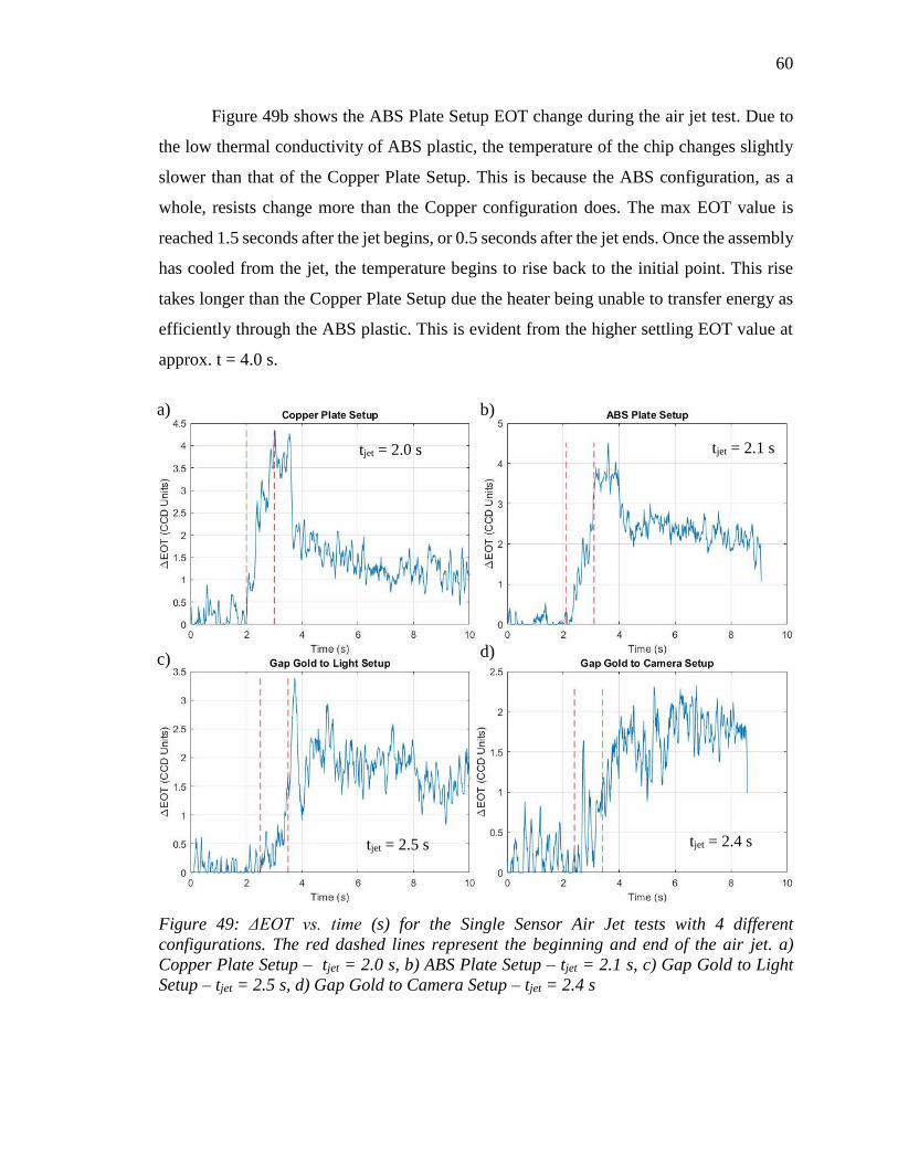
60

Figure 49b shows the ABS Plate Setup EOT change during the air jet test. Due to

the low thermal conductivity of ABS plastic, the temperature of the chip changes slightly

slower than that of the Copper Plate Setup. This is because the ABS configuration, as a

whole, resists change more than the Copper configuration does. The max EOT value is

reached 1.5 seconds after the jet begins, or 0.5 seconds after the jet ends. Once the assembly

has cooled from the jet, the temperature begins to rise back to the initial point. This rise

takes longer than the Copper Plate Setup due the heater being unable to transfer energy as

efficiently through the ABS plastic. This is evident from the higher settling EOT value at

approx. t = 4.0 s.

Figure 49: ΔEOT vs. time (s) for the Single Sensor Air Jet tests with 4 different

configurations. The red dashed lines represent the beginning and end of the air jet. a)

Copper Plate Setup – tjet = 2.0 s, b) ABS Plate Setup – tjet = 2.1 s, c) Gap Gold to Light

Setup – tjet = 2.5 s, d) Gap Gold to Camera Setup – tjet = 2.4 s

a) b)

d) c)

tjet = 2.0 s tjet = 2.1 s

tjet = 2.4 s tjet = 2.5 s

61

Figure 49c shows the Gap Gold to Light Setup EOT change during the air jet test.

This configuration is similar to the ABS Plate Setup with an added layer of PDMS

separating the chip and heater. This extra material prevents the chip from reaching the same

initial temperature as the Copper and ABS configurations (starts at lower temp). As a result,

the change in EOT seen with this assembly is smaller than the previous two. Similar to the

ABS Plate Setup, the rise takes longer than the Copper Plate Setup with the max EOT value

reached 1.25 seconds after the start of the jet. The extra material prevents the chip from

reheating quickly, making the settling EOT value closer to the max EOT value than first

two configurations.

Figure 49d shows the Gap Gold to Camera Setup EOT change during the air jet

test. This configuration is the same as the Gap Gold to Light Setup except the gold side of

the NHA chip is facing the camera. In this figure we observe the thermal reaction on the

opposite side of the air jet. As predicted by the analytical model, the unexposed side of the

chip cools down slower than the exposed side, as depicted by a clear delay in rise time for

the max EOT value. We see the max EOT value reached 4.3 seconds after the beginning

of the jet. This tells us the opposite side of the chip continued to cool well after the jet had

concluded. The total change in EOT is much small than the other 3 cases, meaning the back

side of the chip does not experience the same level of temperature change as the front. This

validates the findings from the analytical model. Interestingly, the settling EOT value is

not much lower than the max value, indicating the back side of the chip did not reheat

quickly despite being closer to the heater. This signifies the effect of the extra PDMS

material.

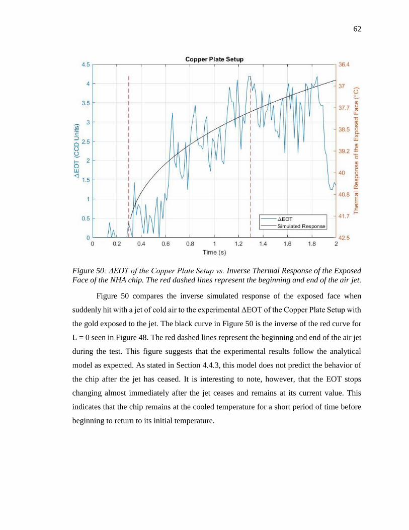
62

Figure 50: ΔEOT of the Copper Plate Setup vs. Inverse Thermal Response of the Exposed

Face of the NHA chip. The red dashed lines represent the beginning and end of the air jet.

Figure 50 compares the inverse simulated response of the exposed face when

suddenly hit with a jet of cold air to the experimental ΔEOT of the Copper Plate Setup with

the gold exposed to the jet. The black curve in Figure 50 is the inverse of the red curve for

L = 0 seen in Figure 48. The red dashed lines represent the beginning and end of the air jet

during the test. This figure suggests that the experimental results follow the analytical

model as expected. As stated in Section 4.4.3, this model does not predict the behavior of

the chip after the jet has ceased. It is interesting to note, however, that the EOT stops

changing almost immediately after the jet ceases and remains at its current value. This

indicates that the chip remains at the cooled temperature for a short period of time before

beginning to return to its initial temperature.

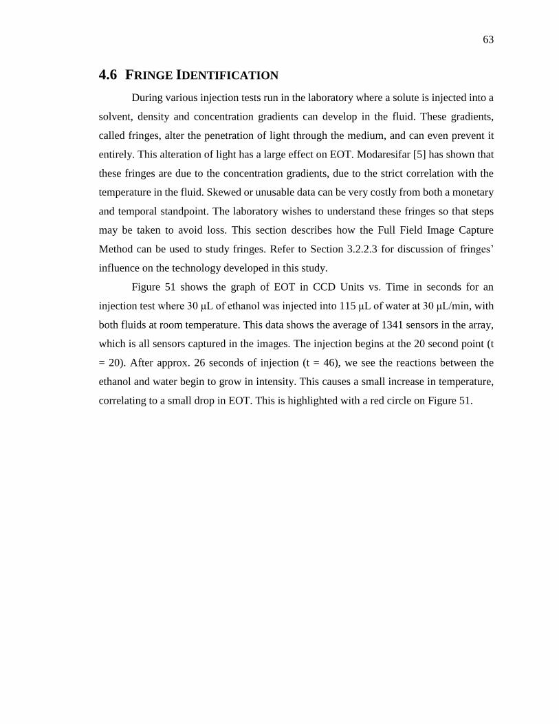
63

4.6 FRINGE IDENTIFICATION

During various injection tests run in the laboratory where a solute is injected into a

solvent, density and concentration gradients can develop in the fluid. These gradients,

called fringes, alter the penetration of light through the medium, and can even prevent it

entirely. This alteration of light has a large effect on EOT. Modaresifar [5] has shown that

these fringes are due to the concentration gradients, due to the strict correlation with the

temperature in the fluid. Skewed or unusable data can be very costly from both a monetary

and temporal standpoint. The laboratory wishes to understand these fringes so that steps

may be taken to avoid loss. This section describes how the Full Field Image Capture

Method can be used to study fringes. Refer to Section 3.2.2.3 for discussion of fringes’

influence on the technology developed in this study.

Figure 51 shows the graph of EOT in CCD Units vs. Time in seconds for an

injection test where 30 μL of ethanol was injected into 115 μL of water at 30 μL/min, with

both fluids at room temperature. This data shows the average of 1341 sensors in the array,

which is all sensors captured in the images. The injection begins at the 20 second point (t

= 20). After approx. 26 seconds of injection (t = 46), we see the reactions between the

ethanol and water begin to grow in intensity. This causes a small increase in temperature,

correlating to a small drop in EOT. This is highlighted with a red circle on Figure 51.

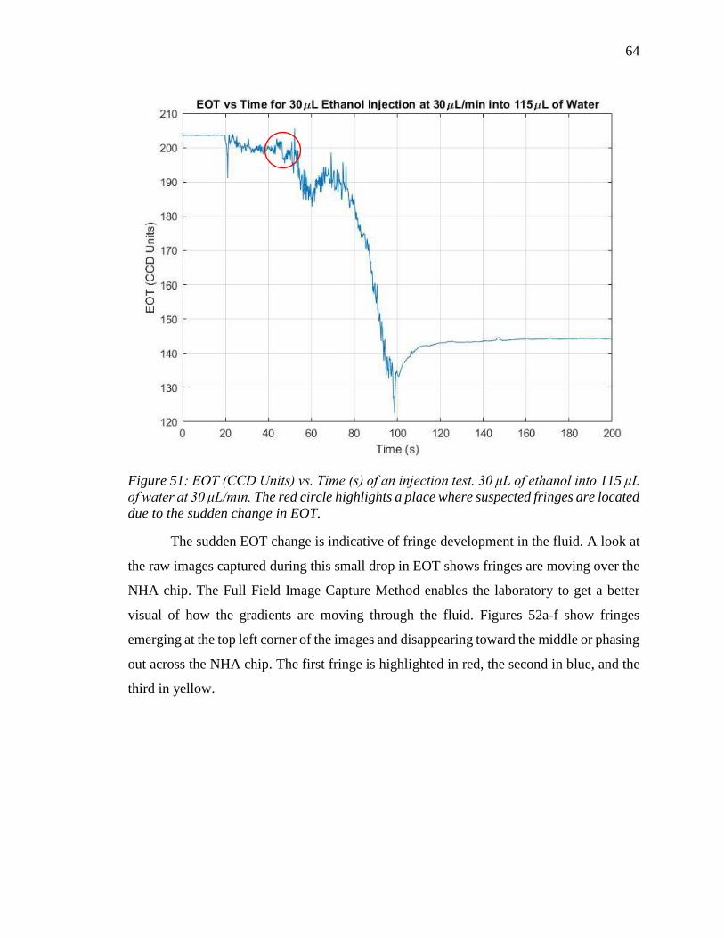
64

Figure 51: EOT (CCD Units) vs. Time (s) of an injection test. 30 μL of ethanol into 115 μL

of water at 30 μL/min. The red circle highlights a place where suspected fringes are located

due to the sudden change in EOT.

The sudden EOT change is indicative of fringe development in the fluid. A look at

the raw images captured during this small drop in EOT shows fringes are moving over the

NHA chip. The Full Field Image Capture Method enables the laboratory to get a better

visual of how the gradients are moving through the fluid. Figures 52a-f show fringes

emerging at the top left corner of the images and disappearing toward the middle or phasing

out across the NHA chip. The first fringe is highlighted in red, the second in blue, and the

third in yellow.

65

a)

b)

c)

(1)

(2)

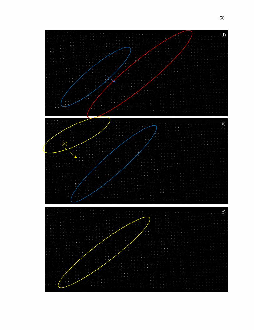
66

d)

e)

f)

(3)

67

Figure 52: Raw data capture during an injection experiment. Fringes are highlighted

moving across the NHA chip in red (1), blue (2), and yellow (3).

The fringes move in this direction across the screen because of the formation of the

experiment. Referring to Figure 16, the ethanol was injected through the right/top inlet. In

these images, gravity acts from left to right, with the top inlet toward the top left of the

image. Another way to think of this is that the CCD camera is rotated 90° clockwise.

Fringes move across the chip very quickly due to the small size of the sensor array. This

makes tracking them very difficult. This test was performed with the whole chip within

view of the camera, which limited the capture frequency to 5.9 Hz overall in this case. At

the beginning of the test the program was running near 7.8 Hz, but slowed as time passed.

A smaller image, and thus faster capture speed, could possibly get a better grasp of

the speed of these fringes. Section 6 discusses possible future work that could track these

to better avoid corrupted data.

5 CONCLUSIONS

The Full Field Image Capture Method (FFICM) for use with the laboratory’s

microscale calorimeter design was developed and tested. This new method was compared

to the Sensor Location Method (SLM), the current method used by the laboratory. It was

found that the FFICM produces equivalent results to the SLM when an identical injection

test is run with both methods. Five sensor locations were chosen and compared

individually, as well as an average of all sensors used in each method. The shapes of the

comparison graphs validate the efficacy of the FFICM.

The FFICM was shown to be able to track sensor locations with time despite

temperature changes to the NHA chip. It was determined that a temperature change of

16.3°C caused a sensor to move 33.94 pixels, or 25.12 μm.

The FFICM demonstrated consistent capture speeds ranging from 3.63 Hz with full

2048x2048 pixel images to 59.93 Hz with 1x1 pixel images. Some experiments reached 65

Hz but were not consistently reproducible. During some experiments, the capture speed

decreased over the time of the experiment.

68

The effect of the number of averaged sensors on overall EOT was demonstrated to

be significant at numbers between 0 and 220. Sensor numbers greater than 220 vary in

consistency and smoothness but share similar shape. The significance of the variation

between lower sensor number validates the necessity of the FFICM.

The FFICM was shown to produce accurate results when the EOT was compared

to a simulation of a cooling semi-infinite solid modeled after the NHA chip. It was also

demonstrated that chip surroundings have a large effect on ΔEOT when the same sensor is

monitored while the chip is exposed to an air jet. The material of the cell assembly plate

changes the reaction of the ΔEOT to air jet, based on its thermal conductivity or ability to

resist temperature change. Greater distance from the cell assembly plate lowered the ΔEOT

of the chip because it prevented the chip from reaching the same initial temperature as the

other configurations. Also, when the gold side, or sensing side, of the NHA chip is faced

away from the jet toward the camera, the ΔEOT is lower and the shape of the ΔEOT curve

is drastically changed.

Lastly, the FFICM was shown to enable the laboratory to begin to track the

movement of fringes in the sensing fluid. EOT vs. Time graphs were used to detect possible

fringe locations in time and then raw captured images were examined to find fringes. This

is only a preliminary step to tracking fringes but the FFICM has been shown to begin this

process.

6 RECOMMENDATIONS AND FUTURE WORK

The tests conducted in Section 4.4 could be improved with a simulation which

included the response of the chip after the air jet ends. It would be interesting to see how

the simulation compares the EOT reaction of the chip array. Also, collecting experimental

temperature data during the blast could provide and even deeper look at the energy transfer

in the chip. The first step, however, would be to automate the air jet to decrease the

uncertainty behind the jet characteristics.

It was attempted to include the calculation of the specific heat of water into this

study, but the lab ran out of time. The experiment introduced room temperature (~24°C)

water into water heated to 40°C while EOT and temperature data were collected. After

69

derivation of equations, creation of calculation programs, and conduction of experiments,

the lab discovered the injection temperature of the water equal to the assumption. The inlet

tube was heating the water to almost 38°C, which drastically change the calculation of

specific heat. To fix this problem, a heat sink to the environment is suggested to be wrapped

around the inlet tube, keeping the tube at room temperature while the chamber is heated to

initial temperature. This should fix the issue, and the calculation should be much closer to

the known value.

The theory behind the programs developed in this study is what makes them novel.

While LabVIEW was chosen as the software used to capture data with the CCD camera in

the experimental setup due to its usability, it is believed to the slow the camera’s capturing

speeds. The camera is rated for 125 Hz by the manufacturer. C++ could be used to rewrite

the capturing programs and possibly increase the overall capture speed. This could enable

greater sensitivity and response for the microscale calorimeter. This would also enable

better ability of the program to track fringes. During the experiments discussed in Section

4.6, the capture frequency was 5.9 Hz. If the whole NHA could visible with a speed 15 Hz,

the fringes could be better analyzed. C++ could also be used to post-process the EOT,

however this would require the creation of a laboratory-specific connected components

algorithm to find the sensors in the images and a separate data acquisition system.

MATLAB was used to write the post-processing programs due to its image

processing toolbox capabilities and the ease of use associated with its language. It could

also be used to control the camera in the experimental setup. The image processing toolbox

is not optimized for the laboratory’s purposes like a C++ program could be, but switching

to one language could save time and labor.

70

REFERENCES

[1] G. K. E. F. John E. Ladbury, "Adding calorimetric data to decision making in

lead discovery: a hot tip," Nature Reviews Drug Discovery 9, pp. 23-27,

January 2010.

[2] E. Freire, "Do enthalpy and entropy distinguish first in class from best in

class?," Drug Discovery Today, vol. 13, pp. 869-874, 2008.

[3] M. Sen, "DESIGN AND DEVELOPMENT OF CALORIMETRIC

BIOSENSORS USING EXTRA ORDINARY OPTICAL TRANSMISSION

THROUGH NANOHOLE ARRAYS," ProQuest Dissertations Publishing,

Boston, MA, 2012.

[4] G. Kowalski, J. Ji, A. Talakoub, M. Sen and D. Larson, "Fast temperature

sensing using changes in extraordinary optical transmission through an array

of subwavelength apertures," Optical Engineering, vol. 48(10), p. 104402, 26

October 2009.

[5] M. Modaresifar and G. Kowalski, "Microscale calorimetric device for

determining reaction parameters," Thermochimica Acta, vol. 655, pp. 137-

144, 2017.

[6] M. Sen, G. Kowalski, J. Fiering and D. Larson, "A continuous flow

microfluidic calorimeter: 3-D numerical modeling with aqueous reactants,"

Thermochimica Acta, vol. 603, pp. 184-196, 2015.

[7] J. Reiter, "CFD ANALYSIS OF EDTA-CACL2 REACTION IN A

MICROFLUIDIC CHANNEL TO AID IN DESIGN OF NOVEL

CALORIMETER DEVICE," Boston, 2015.

71

[8] G. Healthcare, "Resolving a bottleneck in screening and characterization of

recombinant antibody fragments using Biacore 4000," 2010.

[9] V. Kamat and A. Rafique, "Extending the throughput of Biacore 4000

biosensor to accelerate kinetic analysis of antibody-antigen interaction,"

Analytical Biochemistry, vol. 530, pp. 75-86, 1 August 2017.

[10] G. A. Holdgate, "Making cool drugs hot: isothermal titration calorimetry as a

tool to study binding energetics," BioTechniques, vol. 31, no. 1, pp. 164-

166,168,170, 2001.

[11] R. O'Brien and I. Haq, "Application of Biocalorimetry: Binding, Stability,

and Enzyme Kinetics," in Biocalorimetry 2: Applications of Calorimetry in

the Biological Sciences, John Wiley and Sons, Ltd., 2004, pp. 1-34.

[12] K. Vuignier, J. Schappler, J.-L. Veuthey, P.-A. Carrupt and S. Martel, "Drug-

protein binding: a critical review of analytical tools," Analytical and

Bioanalytical Chemistry, vol. 398, no. 1, pp. 53-66, September 2010.

[13] I. Jelesarov and H. R. Bosshard, "Isothermal titration calorimetry and

differential scanning calorimetry as complementary tools to investigate the

energetics of biomolecular recognition," Journal of Molecular Recognition,

vol. 12, no. 1, pp. 3-18, 1999.

[14] E. Freire, "Differential Scanning Calorimetry," Methods in Molecular

Biology, vol. 40, pp. 191-218, 1995.

[15] P. L. Privalov and S. A. Potekhin, "Scanning Microcalorimetry in studying

temperature-induced changes in proteins," Methods in Enzymology, vol. 131,

pp. 4-51, 1986.

[16] G. Healthcare, "MicroCal iTC200 System," GE Healthcare, 2011.

[17] R. H. Ritchie, "Plasma losses by fast electrons in thin films," Physical Review,

vol. 106, no. 5, pp. 874-881, 1957.

[18] J. V. Coe, "Extraordinary Transmission of Metal Films with Arrays of

Subwavelength Holes," Annual Review of Physical Chemistry, vol. 59, pp.

179-202, 2008.

72

[19] W. L. Barnes, A. Dereux and T. W. Ebbesen, "Surface Plasmon

Subwavelength Optics," Nature, vol. 424, pp. 824-830, 14 August 2003.

[20] H. A. Bethe, "Theory of Diffraction by Small Holes," Physical Review, vol.

66, pp. 163-182, 1944.

[21] T. W. Ebbesen, H. J. Lezec, H. F. Ghaemi, T. Thio and P. A. Wolff,

"Extraordinary optical transmission through sub-wavelength hole arrays,"

Nature, vol. 391, pp. 667-669, 12 February 1998.

[22] A. Krishnan and e. al., "Evanescently coupled resonance in surface plasmon

enhanced transmission," Optics Communications, vol. 200, pp. 1-7, 15

December 2001.

[23] P. Stark, A. E. Halleck and D. Larson, "Short order nanohole arrays in metals

for highly sensitive probing of local indices of refraction as the basis for a

highly multiplexed biosensor technology," Methods, vol. 37, pp. 37-47, 2005.

[24] J. Ji and J. G. O'Connell, "High-Throughput Nanohole Array Based System

To Monitor Multiple Binding Events in Real Time," Journal of Analytical

Chemistry, vol. 80, no. 7, pp. 2491-2498, 2008.

[25] J. L. Z. Cerroblanco, "Development of a New Generation of Temperature

Sensors Based on Extraordinary Optical Transmission for Fe-Rh," University

of Guanajuato, Salamanca, 2015.

[26] J. D. Murray and W. V. Ryper, Encyclopedia of Graphics File Formats, 2nd

Edition, O'Reilly Media, 1996.

[27] F. P. Incropera and D. P. D. Witt, Introduction to Heat Transfer, John Wiley

and Sons, Inc., 1985.

[28] J. N. B. Livingood and P. Hrycak, "Impingment Heat Transfer from Turbulent

Air Jets to Flat Plates - A Literature Survey," National Aeronautics and Space

Administration, Cleveland, 1973.

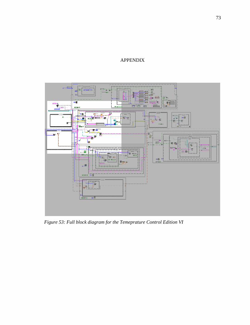
73

APPENDIX

Figure 53: Full block diagram for the Temeprature Control Edition VI

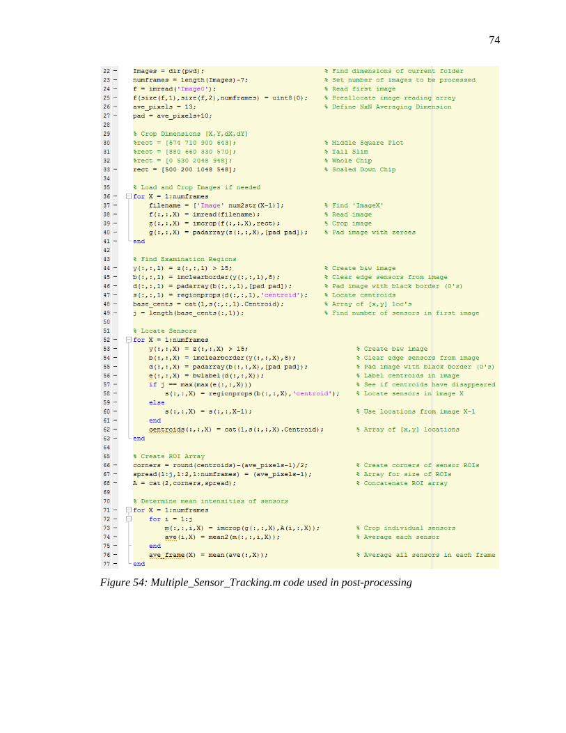
74

Figure 54: Multiple_Sensor_Tracking.m code used in post-processing

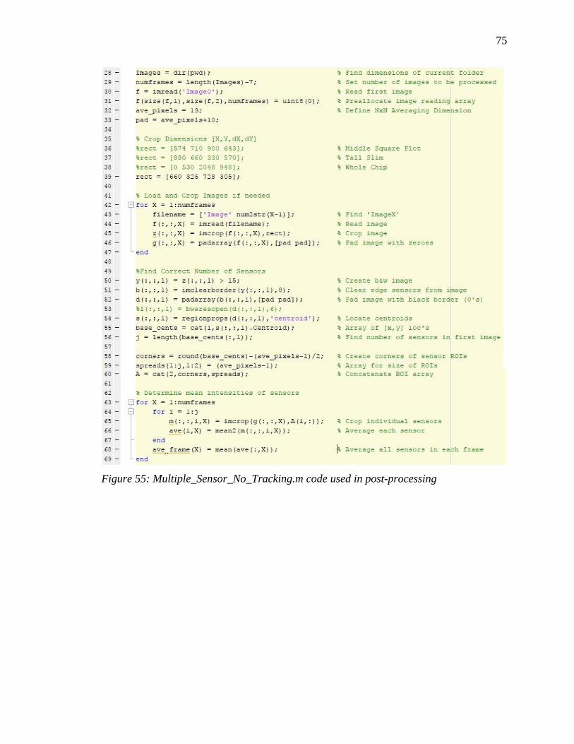
75

Figure 55: Multiple_Sensor_No_Tracking.m code used in post-processing

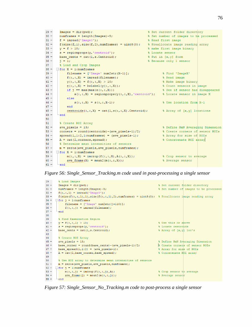
76

Figure 56: Single_Sensor_Tracking.m code used in post-processing a single sensor

Figure 57: Single_Sensor_No_Tracking.m code to post-process a single sensor

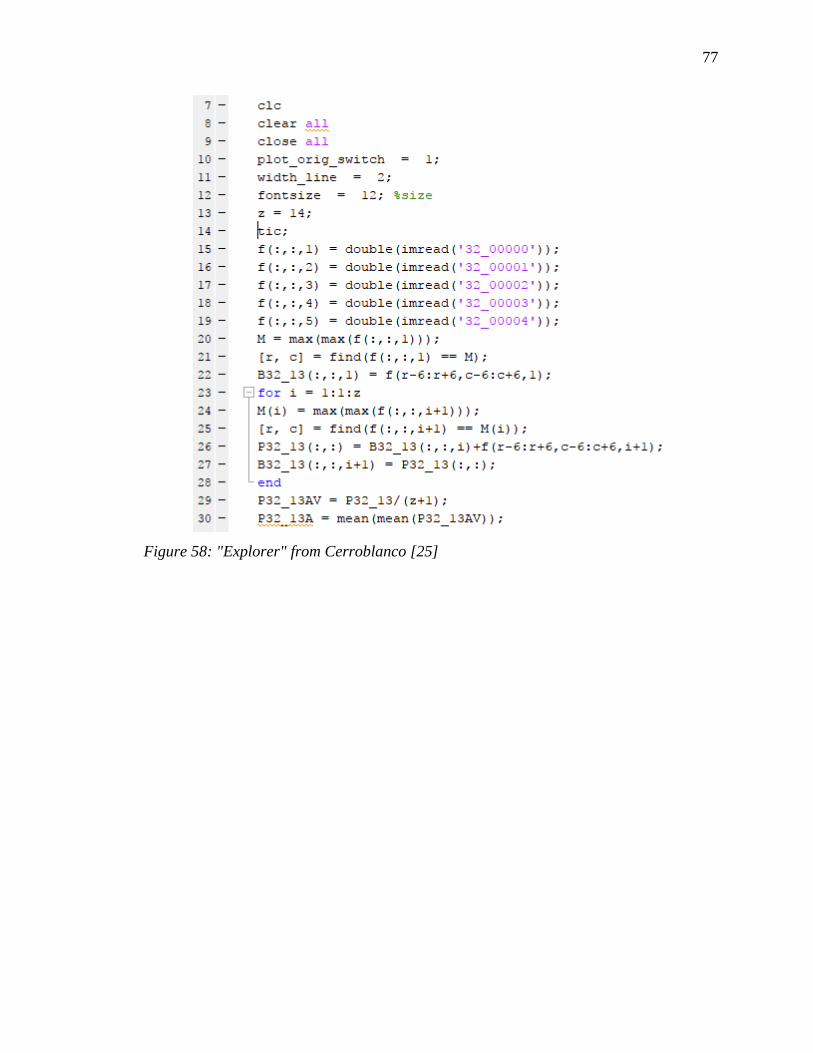
77

Figure 58: "Explorer" from Cerroblanco [25]