improving emergency department performance using discrete
TRANSCRIPT

1
Improving Emergency Department
Performance using Discrete-event and Agent-
based Simulation
By
Arjun Kaushal
A thesis submitted to the Faculty of Graduate Studies of
The University of Manitoba
in partial fulfilment of the requirements for the degree of
MASTER OF SCIENCE
Department of Mechanical Engineering
University of Manitoba
Winnipeg, Manitoba
© Copyright 2014, Arjun Kaushal

2
Abstract
This thesis investigates the causes of the long wait-time for patients in Emergency
department (ED) of Victoria General Hospital, and suggests changes for improvements.
Two prominent simulation techniques have been used to replicate the ED in a simulation
model. These are Discrete-event simulation (DES) and Agent-based modeling (ABM).
While DES provides the basic modeling framework ABM has been used to incorporate
human behaviour in the ED. The patient flow in the ED has been divided into 3 phases:
input, throughput, and output.
Model results show that there could be multiple interventions to reduce time taken to be
seen by the doctor for the first time (also called WTBS) either in the output phase or in
the input phase. The model is able to predict that a reduction in the output phase would
cause reduction in the WTBS but it is not equipped to suggest how this reduction can be
achieved.
To reduce WTBS by making interventions in the input phase this research proposes a
strategy called fast-track treatment (FTT). This strategy helps the model to dynamically
re-allocate resources if needed to alleviate high WTBS. Results show that FTT can
reduce WTBS times by up-to 40%.

3
Glossary
ED Emergency Department
VGH-ED Victoria General hospital-Emergency department
WTBS Patient status when he/she is waiting to be seen by a doctor
LOS Patient length of stay in the ED
VGH-EDsim model Simulation model of the VGH-ED
SD System Dynamics simulation
DES Discrete-event simulation
ABS Agent-based simulation
Monitored beds Beds that have the capacity to continuously monitor patient‘s
vital signs
Non – monitored beds Normal ED beds that do not have monitors.
Monitor – area Bed area that consists of 15 monitored beds.
Treatment – area Bed area that consists of 4 non- monitored beds.
MTA – area Minor treatment area, that consists of 5 non- monitored beds
reserved for least acuity patients.
Input phase Time period between patient arrival till bed allotment.
Throughput phase The time period between bed allotment till the end of treatment.
Output phase The time period between end of treatment till patient discharge.
Admits Patients that are admitted to the hospital upon discharge from

4
ED.
Non-admits Patients that are discharged back into the community.
CTAS Canadian Triage and Acuity Scale
Initial nurse assessment The first nurse assessment after patient is allotted a bed
Initial doctor assessment The first assessment by a doctor. Point where WTBS status ends.
TIP Patient status when treatment is in progress.
Output status Patient’s status when he/she is in output phase.
ERH Patient’s status when he/she is held in the ED for further
monitoring.
TBADM Patient’s status when he/she is waiting for a bed in the main
hospital
PD Patient’s status when he/she is waiting on an ED bed for
miscellaneous reasons.
WBED Component of WTBS where patient is waiting for a bed
WNURSE Component of WTBS where patient is waiting a nurse for an
initial nurse assessment.
WDOCTOR Component of WTBS where patient is waiting a doctor for an
initial doctor assessment.
DBA strategy Dynamic bed-allotment strategy. Agent based strategy to model
human factor involved in bed-allotment decision.
Desired treatment
location Patient’s desired treatment location based on patient’s attributes.
Actual treatment
location
Patient’s actual treatment location based on patient’s desired
treatment location and bed availability.
FTT strategy Fast track treatment strategy. Proposed strategy to improve ED
wait-times.

5
Acknowledgments
I want to extend my gratitude to my adviser Dr. Qingjin Peng. This thesis would not have
been achieved without his precious support and guidance. I would also like to thank Prof.
Trevor Strome and Prof. Erin Weldon for providing me excellent insight into the VGH-
ED and healthcare in general. I would also like to thank the staff members at the
Emergency Department of Victoria General Hospital, especially Mr. Ray Sanchez
Manager of Patient Care for his help in data collection and estimates. This research was
funded by Medical Foundation ER Research.
I would also like to specially mention Dr. Ricardo Lobato de Faria, Chief Medical Officer
at Seven Oaks hospital, whom I worked under during a 13-week internship. His inputs
regarding the ED were invaluable and helped me deepen my understanding about the
health care system in general.
This research was also supported in part by a Western Regional Training Centre
studentship funded by Canadian Institutes of Health Research and Manitoba Health.

6
Dedication
To my parents who have made me what I am. To my wife who was always been there in
my journey of doing this research. To my friends who have been with me through thick
and thin.

7
Contents
1. Introduction ............................................................................................................... 19
1.1. Background ........................................................................................................ 19
1.2. Research Objectives ........................................................................................... 21
1.3. Overview of the research-methodology ............................................................. 22
2. Literature review ....................................................................................................... 25
2.1. ED overcrowding problem - An overview ......................................................... 25
2.2. Different approaches of simulating an ED ......................................................... 26
2.2.1. System Dynamics (SD) ............................................................................... 26
2.2.2. Discrete-event simulation (DES) ................................................................ 27
2.2.3. Agent-based simulation (ABS) ................................................................... 28
2.2.4. Why choose DES over SD? ........................................................................ 29
2.3. Discrete-event simulation in ED ........................................................................ 30
2.3.1. Variable change scenarios........................................................................... 31
2.3.2. Process change scenarios ............................................................................ 33
2.3.3. Miscellaneous scenarios.............................................................................. 36

8
2.4. Discussion of literature....................................................................................... 37
3. Research methodology .............................................................................................. 39
3.1. Phases of research .............................................................................................. 39
3.1.1. Phase-1: Understanding the real ED. .......................................................... 41
3.1.2. Phase-2: Data collection and building the VGH-EDsim model ................. 41
3.1.3. Phase 3: Model analysis and design of solutions ........................................ 42
3.2. Thesis organization ............................................................................................ 42
4. Victoria General Hospital-ED patient flow .............................................................. 44
4.1. Structure of the ED ............................................................................................. 44
4.2. VGH-ED patient flow: the Input-Throughput-Output approach ........................ 46
4.2.1. Input phase .................................................................................................. 46
4.2.2. Throughput phase........................................................................................ 49
4.2.3. Output phase ............................................................................................... 52
4.3. Problem formulation and underlying assumptions............................................. 54
4.3.1. Prima-facie solution .................................................................................... 56
5. Data collection for VGH-EDsim model ................................................................... 57
5.1. Data collection for VGH-EDsim model ............................................................. 57
5.2. Transforming VGH-ED data into model input data ........................................... 59
5.2.1. Arrival data ................................................................................................. 60

9
5.2.2. Patient attribute data ................................................................................... 65
5.2.3. Process time data......................................................................................... 69
6. The Simulation model ............................................................................................... 71
6.1. Introduction to Flexsim 3D simulation software................................................ 71
6.2. Steps to build a DES model for VGH-ED.......................................................... 73
6.2.1. Step1: Deciding the scope of the model ..................................................... 75
6.2.2. Step 2: Designing simulation model logic .................................................. 75
6.2.3. Step 3: Writing the simulation model logic in FlexSim ............................. 83
6.2.4. Step 4: Verification of the model ................................................................ 84
6.2.5. Step 5: Validation of the model .................................................................. 86
6.3. Stages of building VGH-EDsim model .............................................................. 90
6.3.1. Stage 1: Building model with bed resource only ........................................ 91
6.3.2. Stage 2: Building model with bed and nurse resource ................................ 92
6.3.3. Stage 3: Building the model with all three resources. ................................ 93
6.3.4. Analysis of results ....................................................................................... 96
7. Agent-based simulation ............................................................................................ 99
7.1. Need for Agent-based simulation ....................................................................... 99
7.1.1. Shortcomings of DES ................................................................................. 99
7.1.2. Agent and agent-based simulation ............................................................ 100

10
7.1.3. Modeling of an Agent ............................................................................... 102
7.1.4. Need for integration of DES and ABS ...................................................... 103
7.2. Model validation using Agent-based modeling ............................................... 104
7.2.1. Understanding the cause of outliers .......................................................... 104
7.2.2. Dynamic bed-allotment strategy ............................................................... 105
8. Model analysis and solution design for ED improvement ...................................... 117
8.1. Model analysis.................................................................................................. 117
8.1.1. Analysis of Output phase of ED ............................................................... 117
8.1.2. Analysis of Input phase of ED .................................................................. 120
8.2. Fast track treatment (FTT) strategy .................................................................. 122
8.2.1. Simulation model logic for FTT strategy.................................................. 124
8.2.2. Coding for FTT strategy ........................................................................... 128
8.2.3. Results from Fast track treatment strategy................................................ 129
8.2.4. Conclusion of FTT strategy ...................................................................... 133
9. Conclusions and future work .................................................................................. 136
9.1. Research Summary ........................................................................................... 136
9.2. Research contributions ..................................................................................... 136
9.2.1. Patient treatment captured in detail........................................................... 137
9.2.2. Integration of DES and ABS for a statistically validated model .............. 137

11
9.2.3. Flexible process change alternative .......................................................... 138
9.3. Recommendations for the VGH-ED improvement .......................................... 138
9.4. Future work ...................................................................................................... 139
REFERENCES ............................................................................................................... 141
A. User Manual ............................................................................................................ 149
A.1. Model view and control buttons ....................................................................... 150
A.2. Model Input window ........................................................................................ 151
A.2.1. Experiment 1: Change parameters of DBA strategy ................................. 151
A.2.2. Experiment 2: Study the effect of reducing TBADM and ERH times ..... 152
A.2.3. Experiment 3: Run model with Fast track treatment enabled ................... 152
A.3. Model Output window ..................................................................................... 153
A.4. Collecting data from the model ........................................................................ 154
B. Distribution Data ..................................................................................................... 157
B.1. Arrival distributions ......................................................................................... 157
B.2. Treatment time distributions ............................................................................ 158
B.3. Output phase process-time distributions .......................................................... 159

12
List of Tables
Table 5-1 ED resource data............................................................................................... 57
Table 5-2 Hour by Day table (number of patients in an hour of a day) ............................ 61
Table 5-3 Hour by Weekday occurrence table (number of patients in an hour of a day) . 62
Table 5-4 Hour by Weekday table (average number of patients in an hour of a weekday)
........................................................................................................................................... 62
Table 5-5 Inter-arrival time table (in minutes) ................................................................. 63
Table 5-6 Age group based on arrival mode ..................................................................... 66
Table 5-7 Percentages of CTAS based on arrival mode and age ...................................... 67
Table 5-8 Treatment location percentages based on CTAS .............................................. 68
Table 5-9 Discharge disposition probability percentages based on Age .......................... 69
Table 6-1 Comparison of average wait-times and length of stay (time in minutes) ......... 93
Table 6-2 Normality test results for all data samples ....................................................... 94
Table 6-3 Mann-Whitney U test results for VGH-EDsim model built using DES only .. 95
Table 7-1 Actual and desired treatment location percentages ........................................ 104
Table 7-2 Possible values of all state variables for database agent ................................ 107
Table 7-3 Treatment location percentages (Nurse Dilemma = 30%-40%)..................... 114

13
Table 7-4 Comparison of average wait-times, processing times and length of stay (Nurse
dilemma = 30%-40%) ..................................................................................................... 114
Table 7-5 Mann Whitney u test results for VGH-EDsim model built using DBA strategy
......................................................................................................................................... 115
Table 8-1 Percentage reduction in WTBS (local best at each T) .................................... 134

14
List of Figures
Figure 1-1 Overview of research Methodology [13] ........................................................ 24
Figure 3-1 Research Methodology.................................................................................... 40
Figure 4-1 VGH-ED layout .............................................................................................. 45
Figure 4-2 Input Phase of patient flow in VGH ED ......................................................... 48
Figure 4-3 Throughput phase of patient flow in VGH-ED ............................................... 50
Figure 4-4 Output phase of patient flow in VGH-ED....................................................... 53
Figure 4-5 Activities and wait-times in the VGH-ED ...................................................... 55
Figure 5-1 Arrival rate for walk-in and ambulance patients ............................................. 64
Figure 6-1 Model building process-flowchart .................................................................. 74
Figure 6-2 Snapshot of VGH-EDsim model ..................................................................... 76
Figure 6-3 Input phase of simulation model logic ............................................................ 77
Figure 6-4 Throughput phase of simulation model logic.................................................. 79
Figure 6-5 Output phase of simulation model logic ......................................................... 81
Figure 6-6 Activity flow within treatment phase .............................................................. 82
Figure 6-7 Steady state analysis for a typical VGH-EDsim model run ............................ 90
Figure 6-8 Frequency distribution histogram to compare model output data with model
validation data (DES model) ............................................................................................. 97

15
Figure 7-1 Example of a Moore machine [63]................................................................ 103
Figure 7-2 Simulation model for Dynamic bed-allotment strategy ................................ 111
Figure 7-3 Frequency distribution histogram to compare model output data with model
validation data (Model with DBA strategy).................................................................... 116
Figure 8-1 Percentage reduction in WTBS at different levels of reduction in ERH and
TBADM times ................................................................................................................ 118
Figure 8-2 Breaking down WTBS into its components .................................................. 120
Figure 8-3 Model output: WBED time broken into time intervals for all CTAS types .... 121
Figure 8-4 TIP times for CTAS 4 and 5 broken into time intervals ............................... 122
Figure 8-5 Simulation logic for Fast track treatment strategy part 1 .............................. 125
Figure 8-6 Simulation logic for Fast track treatment strategy part 2 .............................. 126
Figure 8-7 Average WTBS time and LOS time plot versus ceiling value (at threshold=
50) ................................................................................................................................... 130
Figure 8-8 Percentage of time fast track treatment strategy is implemented versus ceiling
limit value (at threshold = 50) ......................................................................................... 130
Figure 8-9 Average WTBS time versus ceiling value (at threshold = 50,100,150,200). 132
Figure 8-10 Average LOS time versus ceiling value (at threshold = 50,100,150,200) .. 133
Figure 8-11 Range of ceiling in which threshold has maximum impact on WTBS ....... 134
Figure 8-12 Model output using fast track treatment strategy: WTBS time broken into
time intervals for all CTAS types ...................................... Error! Bookmark not defined.
Figure A-1 Model control GUI ....................................................................................... 149
Figure A-2 Model view ................................................................................................... 150
Figure A-3 Model control buttons .................................................................................. 150

16
Figure A-4 Model Input window .................................................................................... 151
Figure A-5 Change nurse dilemma values to change the parameters of DBA strategy . 152
Figure A-6 Enter reduction values to see their effect on WTBS and LOS ..................... 152
Figure A-7 Change FTT parameters ............................................................................... 153
Figure A-8 Model output window .................................................................................. 153
Figure A-9 Controls to record model data ...................................................................... 154
Figure A-10 Model Output data table ............................................................................. 155
Figure A-11 FlexSim’s debugging window .................................................................... 156

17
List of Algorithms
Algorithm 7-1. Charge nurse/decision agent working on the entry trigger of guide-queue
............................................................................................ Error! Bookmark not defined.
Algorithm 7-2. Decision agent working on the message trigger of Hold-queue ....... Error!
Bookmark not defined.
Algorithm 8-1 Database agent evaluating to turn the FTT trigger ON/OFF ............. Error!
Bookmark not defined.
Algorithm 8-2 Hold queue evaluating which patients to release to the fast track area
............................................................................................ Error! Bookmark not defined.

18
List of Appendices
Appendix B-1 Arrival Distributions based on time of day Error! Bookmark not defined.
Appendix B-2 Treatment distributions based on age and arrival mode .. Error! Bookmark
not defined.
Appendix B-3 Output phase process time distributions .... Error! Bookmark not defined.

19
1.Introduction
1.1. Background
Health care expenditure accounts for a major part of Canada’s GDP. Canadian Institute
for health information (CIHI) reported that health care accounts for 11.9% of the total
GDP in 2010 which is an all-time high [1]. In the last decade, total health expenditure in
Canada doubled from close to $100 billion to just over $200 billion [2]. In Manitoba
alone health care costs have increased by over 90% from 2001 to 2011 [3] for only a 9%
increase in the population. This continuous growth trend in health care costs is a
worrying factor for the government and for the society. The problem is complicated by
the fact that the high expenditure has not necessarily led to a better health care system.
High wait-times are a common phenomenon in our health care system and waiting for
care is still the number one barrier in access to health care [4].
Reducing wait-times was identified as a priority by the First ministers in 2004 in the 10-
year plan for strengthening the health care system [5]. In recent years wait-times have
improved or remained steady in many areas but CIHI admits that long wait-times in
emergency department (ED) still remain a challenge to our health care system [6].

20
When studying wait-times in EDs, a commonly used term is ED overcrowding which has
been defined by Canadian Association of Emergency Medicine as:
“ED overcrowding is defined as a situation in which demand for service exceeds the
ability to provide care within a reasonable time, causing physicians and nurses to be
unable to provide quality care [7].”
This definition helps to sum up all the different wait-times in ED, which may be waiting
to see a doctor, time to be seen by a consultant or waiting to get an inpatient bed [7]. In a
nutshell it can be said that if any of these wait-times are longer than usual the ED is
overcrowded.
Simulation has been used previously in many areas of health care. In the case of ED,
simulation provides a technique to build a replica of the real system, such that the model
is reasonably close to reality and can be used to study the effect of different process
alternatives. It is particularly useful for decision makers to test any prospective
alternatives on the model instead of the actual system.
Another major benefit of using simulation is that it can help identify the bottlenecks in a
system. Different EDs serve to different kinds of populations and have different amounts
of resources and staffing. Working protocols may also differ and hence there are no
universal solutions or process alternatives to solve the ED overcrowding problem. For
this research we consider the ED of the Victoria General Hospital (VGH), a community
hospital located in south Winnipeg, Canada. The Emergency Department at the Victoria
general hospital (VGH-ED/ED) provides comprehensive emergency services 24 hours a

21
day and is equipped to treat injuries and illnesses in all age groups. More than 100
patients present to the Emergency Department each day. The ED was renovated in 1982
and was initially designed to treatment 15,000 patients per year, however, that number
has more than doubled by 2013 [8]. This has led to increased pressure on the existing
facility and is leading to long wait- times.
1.2. Research Objectives
The broader objective of this research is to improve the performance of VGH-ED.
Waiting to be seen (WTBS) by a doctor and length of stay (LOS) in the ED are used as
the two performance measures.
An ED is not an isolated entity in the health-care system. Its performance is directly
impacted by the upstream and downstream elements. However in this study the focus is
specifically on the ED itself. This research looks at a micro-level of the isolated ED. The
goal is to find operational level alternatives within the ED and not macro level policy
alternatives.
An ED can be viewed as a discontinuous system, i.e. the system moves from one event to
the next and the system state changes only at these events [9]. For example, when a
patient arrives in the ED, it increases the number of patients in the waiting room causing
a change in the system. However no further change occurs until the registration process
starts. Thus arrival and registration are two discrete events and the system does not
change between these two events.

22
An ED is also a very complex system. These complexities arise due random arrivals,
uncertain service times in providing care and randomness in decision- making due to the
involvement of humans. For example, some doctors are confident to make decisions on a
patient’s treatment based on their own judgment while others might want to order
multiple lab tests and consult specialists for making major decisions.
The precise aim of this research is as follows:
1. To develop an accurate simulation model that is as close to reality as possible
with dynamic human decision-making factors.
2. To utilize this model to study bottlenecks in the current patient flow.
3. To design and test alternatives around these bottlenecks, to help in reducing
WTBS and LOS times.
1.3. Overview of the research-methodology
Discrete-event simulation (DES) is a tool which can be used to model discontinuous
systems such as the ED. By definition a DES model is one which changes state only at
discrete and possibly random events for which probabilities are decided while building
the model. A DES model consists of entities and resources [10]. For example, in case of
ED the entity is patients which require resources such as beds, nurses and doctors to be
treated and discharged from the system.
Although DES is a good tool to simulate multiple events happening in the system at the
same time [10], the downside is that the behavior of entities and resources is static and
does not change as the simulation runs [11]. This makes DES an insufficient tool to

23
model ever changing human behavior in the ED. In order to model these human-decision
making factors, agent-based modeling (ABM) approach can be used.
In general, agent-based modeling and simulation (ABMS) is used to study complex
systems that include decision- making entities and resources. In contrast to DES model
the behavior of the entities and resources is dynamic and changes according to the state
of the system [11]. In an agent-based simulation (ABS) model the system changes the
behavior of entities and resources and they in turn cause the system to change as per their
behavior [12]. Using the previous example, patients, nurses, beds, doctors etc. are now
dynamic and decision-making entities. In an ABS model these dynamic, decision-
making entities are called as agents [11].
Figure 1.1 shows an overview of the research methodology adapted from [13]. In the first
step of this research, the functioning of the ED needs to be understood. Based on this
understanding, a conceptual model is designed. However not every aspect of the ED can
be included in the simulation model either because it is too complex or because it is too
trivial. Therefore a set of assumptions is made so that the ED can be represented by the
simulation model. The conceptual model is validated by the ED managers to ensure that
it is a sufficiently accurate abstraction of the reality. This process is iterative, i.e. more
understanding of the system would be required if the conceptual model is rejected by the
ED managers. This conceptual model is then used to build a simulation model using a
simulation language or software. In this research, a DES software package called Flexsim
is used. It has its own coding language called Flexscript which is quite similar to C++
[14]. The model is verified to ensure that it has been built correctly and that there are no
bugs or syntax errors in the code. This model is then validated to ensure that it represents

24
reality. Similar to conceptual model validation, this too is an iterative process and
assumptions that were made earlier are modified until a validated model is obtained. This
model can then be used to design and test alternatives which can then be applied to the
real-world system.
Figure 1-1 Overview of research Methodology [13]
Conceptual Model Simulation Model
Emergency
Department
Conceptual model
validation
Model
verification
Building
simulation
model
Simulation model
validation
System
analysis and
making
assumptions
Design of
alternatives

25
2.Literature review
The first section of this chapter looks into the system-wide nature of the ED
overcrowding problem. The second section focuses on the most common simulation
methodologies found in literature. The third and fourth sections are dedicated to the
literature review of Discrete-event simulation and its discussion, respectively.
2.1. ED overcrowding problem - An overview
The definition of the ED overcrowding discussed in Chapter 1 defines it as a situation
when patients in the ED experience long wait-times whether before, during or after
treatment [7]. A series of reports was published by the Canadian Agency for Drugs and
Technologies in Health (CADTH) which dealt with measuring overcrowding,
determining the impact of overcrowding on health standards and the interventions
required at a policy level to reduce it [15-18]. In all the reports in this series it has been
repeatedly mentioned that ED overcrowding is a system-wide issue with multiple causes
and with no simple or immediate solutions [18]. However research only focuses on the
ED, its problems and bottlenecks.

26
2.2. Different approaches of simulating an ED
Simulation is one of the most common operations research (OR) techniques used to
model an ED. It is the process of creating a computerized mathematical model of a
physical system which can be used to gain insights about it [9]. It is particularly useful
for experimentation and for identification of bottlenecks in compressed time. A
simulation model comprises of entities flowing/moving from one point to another in the
model and they may be discrete or continuous depending upon the nature of the problem
and the simulation modeling technique being used [9, 19].
A simple search with the words “Emergency Department” and “simulation” in any of the
major databases reveals many papers on this topic. Most common simulation techniques
found in literature are system dynamics (SD), Discrete-event simulation (DES) and
agent-based simulation (ABS). Before choosing the appropriate strategy to model the
VGH-ED it is important to understand these modeling techniques.
2.2.1. System Dynamics (SD)
System dynamics is an analytical modeling methodology to provide a macro level
viewpoint of complex problems [20]. The entities in a SD model are continuous and thus
the system state changes continuously [19]. It combines the qualitative and quantitative
aspects of problem understanding and solving. A qualitative diagram is a causal diagram
and its purpose is to demonstrate the positive and negative impacts of a new decision
[21]. To generate quantitative results a stock flow diagram is generated and a computer
simulation software like STELLA is used to model the system [19].

27
System dynamics has been used in health care for macroscopic system level research. In
a Canadian example, an SD research was carried out by Wong et al [21] in a Toronto
hospital to model the effects of altering patient population entering the ED, altering
resource allocation and making long-term policy level changes. A detailed study was
done by Lane et al to study the effect of reducing bed capacity in hospitals to patient
wait-times in accident and emergency (A&E) units across UK’s National health systems
(NHS) which showed how it can adversely affect wait-times in ED [22]. In another
example, a system level research was conducted using SD strategy to study the effect of
different proposed policy level changes on healthcare affordability in Singapore [23].
2.2.2. Discrete-event simulation (DES)
A Discrete-event simulation model is visualized as consisting of discrete units of entities
that move (flow) through the system [10]. A simulation model consists of one or more
source that creates raw entities and one or more sink that destroys processed entities. In
this journey from source to sink the entities need to go through one or more number of
processes. For this the entities also require resources such as processing stations and
operators which process the entities at these stations and move them from one station to
another. In a typical simulation model several entities may be processed simultaneously
at different stations at any given point of time. If the resources are limited in numbers the
entities have to wait in between in queues. Every time an entity interacts with the system
or the resources an event occurs. The modeller can write specific codes on any of these
events to decide the further course of the entity in the system. Therefore it is said that in a
DES model the system state changes only at discrete but possibly random events in time

28
[9, 10]. For example in a DES model for an ED when a patient (entity) gets triaged
(process) it may be triaged (event) as a minor patient or a major patient based on the
probability modeled by the modeller. If a bed and nurse (resources) are available, the
patient can go to the bed; otherwise he or she has to wait in a waiting room (queue).
A DES study begins by the problem formulation and formally agreeing to the number and
nature of entities in the target system. This is followed by a conceptual model which is
akin to a causal or influence diagram of SD in regards with providing the qualitative
analysis [19]. However the conceptual model in DES focuses on the target entities and
their flow in the system rather than focusing on the driving influences. More about DES
modeling used in the case of VGH ED will be explained in Chapter 3.
2.2.3. Agent-based simulation (ABS)
To understand the concept of agent-based modeling it is necessary to understand the term
agent first. In general terms an agent can be described as an autonomous entity which
makes decisions based on a set of rules [12].The agent also communicates with other
agents within that system and can adapt and change its behavior based on the outcomes
of those interactions. The outcome of a purely ABS model is based on the outcomes of
these interactions [24]. An ABS model has three main aspects:
1.) Agents, their characteristics and behavior.
2.) Relationship between agents, their methods, the probability of their interaction and
outcomes of their interactions.
3.) Agent’s environment. This in some cases can be seen as the manger agent, i.e. the
agent that manages all the other agents towards a specific goal.

29
In this research ABS has been used to enhance the DES model and to study the human
factors. The detailed study and literature review will be discussed in Chapter 7 after
presenting the DES simulation results in Chapter 6.
2.2.4. Why choose DES over SD?
Before comparing the SD to DES methodologies it is important to notice that DES is
purely a simulation methodology and unlike system dynamics that does not have a
qualitative aspect. Essentially, it should only be compared with the quantitative aspect of
system dynamics. Unlike flow diagrams in SD which view “entities” as a continuous
quantity, like a fluid, flowing through a system of reservoirs or tanks connected by pipes,
DES considers the system to be made of individual entities which pass through a series of
activities or processes and in between these activities where they wait in queues. The
state of the system changes at discrete points of time [19].
A number of studies have been carried out comparing SD with DES. The most common
argument found in literature is that SD is more useful where a more holistic and broader
view of the system is taken and DES suits well where an operational understanding of the
system is required [19, 25, 26]. Although some researchers argued that SD models were
better because of their transparency [27], this argument seemed to be valid only for
qualitative SD models. as quantitative SD models with their complex differential
equations, its mathematical models lack the transparency [19]. SD modeling strategy is
argued to be more suitable for modeling fuzzy ambiguous systems whereas DES is
suitable for clearly detailed systems [28]. In general, it has been established that DES is
more suitable where the system is random and changes significantly, in contrast with SD

30
which is more suitable where the system does not react immediately [29]. In other words,
problems that are caused by the system structure are better analyzed by SD, and problems
that are caused by the randomness inside the system are better modeled by DES [28].
From the perspective of the problem nature, most researchers are of the view that SD is
suitable for strategic problems and DES is more suited to operational and tactical
problems [19, 27].
This research focuses on modeling the ED considering it as an isolated system. The
system boundaries are from patient arrival to patient discharge and the patient undergoes
several discrete processes during this journey. The goal is to find bottlenecks within the
ED and solutions proposed will be of operational and tactical level and not policy level.
Therefore considering the characteristics of the system under study, DES methodology is
chosen over SD as the modeling technique. The next section is for the literature review of
DES.
2.3. Discrete-event simulation in ED
Discrete-event simulation is one of the most common methodologies used to model
emergency departments. The literature is full of such examples. Jurishica discusses a
generic process for developing simulation models for EDs [30]. She presented that
alternate scenarios tested on simulation models called as “What-if” scenarios with two
categories: variable change scenario and process change scenario. The former deals with
finding the optimal resource mix in the ED, for example the number of nurses, physicians

31
or beds etc. Process changes could either mean replacing processes with alternate
processes or changing the entire patient flow according to some new strategy.
The review is divided into three sub-sections. Papers that explore variable change
scenarios are discussed in the first subsection, papers that look into process change
scenarios are included in the second sub-section. A third sub-section is to present papers
that do not fall under of any above two categories but are important research to be
discussed.
2.3.1. Variable change scenarios
Many researchers have used DES models to find the optimal resource mix or the optimal
staffing schedule [31-37]. While most researchers tried to design the scenarios as
suggested by ED managers, a few researchers combined some kind of an optimization
technique to find an optimal solution. The variable change scenarios can be further
classified as those which tried to find a more robust staffing schedule i.e. reshuffling of
existing resources and modeling of the effect of additional resources.
Duguay & Chetouane modeled an ED in New Brunswick, Canada and tested different
resource mixes of physicians, nurses and examination rooms [31]. Five alternatives were
designed and each of them had one additional nurse and physicians at different times of
the day. Two of the alternatives also considered one extra bed; however research showed
that adding beds was insignificant to wait-times and simply adding a nurse and a doctor
during busy hours can significantly affect wait-times and throughput. The results showed
that adding these resources shortened wait-times only by around 10%. Paul & Lin also
found out that adding a physician at busy times of the day improves average daily

32
throughput [32]. Similarly, Shim & Kumar used DES to model the effect of adding
another payment station in a Singapore ED [33]. As an example of a major addition of
resources (beds in this case), Kolb et al [34] used simulation DES model to test five
patient buffer scenarios. The buffers were “bed areas” added for specific kinds of
patients. First was “Holding area” for patients that were waiting for inpatient beds,
second was an “ED-discharge lounge” for patients waiting to be discharged and third was
an “Observation Unit” for keeping patients under observation within the ED. The fourth
buffer scenario was a combination of first and second and fifth buffer scenario was the
combination of first, second and third. The results showed that ED performance was
improved in all of the five scenarios but scenarios 4 and 5 were better than the other 3.
Some researchers used optimization techniques such as Genetic algorithm (GA) and
balance scorecard (BS) to find the optimal resource schedule or resource mix. Yi & Lin
improved the quality of care of an ED using a combination of simulation model and GA
[35]. The aim of this research was to find an optimal nurse roster using GA while also
looking to minimize wait-times being simulated by the DES model. The GA model
selects the feasibility of a nurse roster and the DES model checks it for minimum wait-
times. The nurse roster found using this method could reduce wait-times for patients by
approximately 43%. Ismail et al used DES integrated with BS method [36], which
identified that the ED comprises of several queues and wait-times are distributed across
these queues. Three scenarios were tested to balance wait-times across all queues and
reduce the total average wait-times while keeping LOS constant or less. In the first
scenario a nurse was added at Triage. In the second scenario the capacity of the waiting
room was increased. In the third scenario, resources were dynamically distributed in the

33
ED such that the average wait-times in each of the queues remain equal. The first two
scenarios reduced waiting-times at Triage but ended up causing uneven wait-times in the
rest of the ED. Moreover since the first two scenarios also meant adding resources (costs),
the third alternative of dynamic resource relocation was found out to be the best as it
balanced wait-times across the ED and also reduced the rate of patients leaving without
being seen. Thus instead of adding permanent resources, a different rule for optimal
resource distribution was chosen to improve the performance of the ED.
A special mention should be given to Weng et al as it is one of the very few papers that
discuss the cyclic nature of the treatment process [37]. They used the data envelopment
technique to calculate the percentage probability of the number of lab and treatment
cycles that a patient goes through and also the service time distributions for each cycle.
They further used this simulation model to test 32 different combinations of nurses, beds,
and doctors, benchmarked them with an efficiency score which was a combination of
lower wait-times and higher resource utilization.
2.3.2. Process change scenarios
The second set of DES studies is segregated based on process sequence changes [38-45].
Some changed only the order of specific processes while others completely overhaul the
existing process.
Five papers are found that alter some specific process in the ED [38-42]. For example,
Holm and Dahl studied the effect of using an alternate process sequence in the ED [38].
They studied the effect of physician at triage and found that although it did not have a
major impact on wait-times or LOS; it did considerably reduce the time from patient’s

34
arrival to the first meeting with the physician. Thus they argued that a qualitative
improvement was achieved without having any ill effects on the average LOS. Similarly
Ruohonen and Teittinen carried out a simulation study for studying the effect of a triage
process called as the “Triage team method” [39]. The study found that if the triage is
done by a team comprising of a physician, a nurse and a receptionist, the average
throughput time is decreased by 26% due to the fact that lab tests can be ordered at triage
itself. Connelly and Bair built a simulation model and tried the triage concept called
acuity ratio triage to solve the problem of high wait-times for low acuity patients [40].
Using this concept, each care provider was assigned a set ratio of high acuity to low
acuity patients. Preliminary results demonstrated an overall decrease in service times
across all patients.
In another example, Beck et al built a simulation model using DES to study the effect of
an alternate process sequence in the ED “Bedside Registration”, where the registration of
the patient was done alongside treatment [41]. However, they found that the alternate
process worsened the LOS as each patient ended up occupying the bed longer resulting in
scarcity of beds. Zeng et al introduced the concept of team nursing to better distribute the
nurse resource across the beds [42]. As compared to three beds for one nurse, the
responsibility was distributed as per 6 beds for 2 nurses. The result was an improvement
of 13-26% in WTBS and reduction of LOS and LWBS.
There are some examples of complete process reengineering. For instance, Hay et al
argued that flow in the ED should be process driven instead of being patient driven [43].
The research considered that processes and their sequences can be fixed based on
whether the patient is critical or non-critical. These sequences were called “Care

35
pathways”. The order for patients to enter the care pathways was determined by a
dynamic variable called “operating priority” based on the clinical condition of the patient,
which was modified by the time when the patient has already waited in the ED. The
physician resources were allocated to these pathways and patients based on their “Skill-
sets”. The research found that this methodology improved overall patient wait-times and
staff utilization.
Konrad et al also modeled the effects of a major overhaul in the process sequence of the
ED [44]. The traditional system was a sequential system where patients were seen on the
basis of arrival time and acuity. The resources were shared between the major area and
the fast track area, thus it was a sequential flow. This patient flow was replaced by a
concept called split-flow, where the minor patients are sent to continuous care area and
the resources required to treat them are independent of the major area. Thus it turns the
ED into a parallel flow. The base case scenario tested for split-flow showed drastic
reduction in WTBS times and LOS. The model was further tested for sensitivity to arrival
rate and redistribution of patient acuity. In another example of a parallel patient flow,
Davies used simulation to demonstrate that non-critical emergent patients (minor
patients) should be assessed and discharged by the doctor or a nurse practitioner, and be
sent to nurses only for treatment [45]. This system replaced the conventional order of
nurse assessment followed by doctor assessment and then treatment. The conventional
order was followed for critical patients only. The study demonstrated the average wait-
time was reduced up to 3 times following this methodology.

36
2.3.3. Miscellaneous scenarios
This subsection reviews the literature of DES that could not be assigned to either of the
first two sub-sections [46-50]. It is important to discuss them as they show the range of
alternatives with a DES model.
An interesting study by Marmor et al used simulation to build a real-time decision
support system for the ED [46]. The support system helped interpreting current state to
forecast short-term future state of the model. It also assisted ED managers to schedule
staff optimally based on the forecasts.
Holm and Dahl simulated the effect of a 45% increase in patient volumes and predicted
that with the same number of resources the average LOS will increase by 150% [47].
They also found an optimal mix of resources by a hit and trial method, which would
nullify the effect of increase in patient volume on the LOS.
Eskandari et al developed a simulation model for an ED in Iran and tested 14 different
scenarios, comprising of variable change scenarios, process change scenarios and one
hybrid scenario [48]. TOPSIS weighing technique was used to determine the best
scenario and the hybrid scenario was selected as the best.
Gunal and Pidd focused their research on modeling the effect of physician multi-tasking.
A physician resource was divided into “M” mini-physicians to model the fact that a
physician can take care of more than one patient at a time [49]. The study also modeled
the effect of slow and fast doctors on the patient flow.
The study conducted by Ferrand et al was to find an optimal operation room (OR)
allocation strategy for elective and emergency surgeries [50]. The choice was between a

37
flexible strategy where electives and emergent patients had access to all OR beds on first-
come-first-serve basis and a focused strategy where a certain number of beds were
allocated to emergent patients only while the rest were open for electives. The study
found that the focused strategy benefits elective patients but leads to an increase in wait-
times for emergency patients.
2.4. Discussion of literature
There are several conclusions that can be drawn from the literature review. Also there are
certain gaps in the literature which can be addressed in this study.
Most of the papers have described the treatment process as a single process which is an
inaccurate representation (discussed in Chapter 4 in detail). Only Weng et al. [37] have
discussed the cyclic nature of the treatment process.
In most of the variable change scenarios, research seems to point to the fact the adding
resources does not necessarily improve the performance. Even where human resources
need to be added, the proper scheduling has a bigger impact on performance
improvement. Thus it can be said that in the majority of cases resource
relocation/redistribution should be tried before adding resources permanently to the ED.
The process change scenarios show wider variability in results. While in some cases
alternate process flows designed on anecdotal evidence improved the ED, in some cases
they caused loss of performance. Also researchers argue that a complete overhaul in
process sequence is difficult to achieve as it is tough to convince all stakeholders to
implement such a major change. The conclusion to be drawn from the review of process

38
change scenarios is that process reengineering alternatives have different effects on
different EDs. Moreover since none of the process change scenarios were Canadian
studies, therefore any results no matter how good should be carefully considered in the
Canadian context.
Some interesting conclusions can be drawn from some of the miscellaneous papers. For
example, one conclusion to be drawn is that simulation models can be used to simulate
the short-term [46] and long-term [47] state of the system. Thus DES models may also
form the basis of a system level policy change in the long run. The study from Eskandari
et al shows that variable changes can also be accompanied with process change scenarios
to achieve better results than either of them being used alone [48]. The study from Gunal
and Pidd is one of the rare examples for DES used to model the effect of human
performance on ED performance [49]. Although its scope was limited, this study can be
used as a basis to further look into the role of human factors in the ED.
To conclude, in this research the above mentioned gaps shall be filled. The aim of this
research will be to design different solutions to improve the ED, based upon a validated
simulation model which considers the cyclic nature of the treatment process and the
human factors that affect the patient flow in the ED. Since no two EDs are the same,
alternatives will be designed to specifically suit the VGH-ED.

39
3.Research methodology
This chapter introduces the detailed research methodology. The order of the following
chapters is based on the steps mentioned in the research methodology. The concept of
research methodology was introduced briefly in Section 1.3 and this chapter is based on
that introduction.
3.1. Phases of research
This research can be divided into three phases. First phase deals with identifying and
defining the problem and then gaining insight into it. In the second phase, data are
collected from the real system and analyzed. These data are used to build a verified and
validated simulation model called the VGH-EDsim model (or ‘the model’). In the third
phase, the results from the model are used for model analysis and solution design. The
improvements for VGH-ED are suggested on the basis of these experiments. A detailed
flowchart of the different phases is shown in Figure 3.1.

40
Figure 3-1 Research Methodology
Real Emergency Department
Gain system
understanding
Problem formulation and
setting the boundaries of
the system to be modeled
Build conceptual model
Conceptual Model
validated by ED
managers
Data collection as per
conceptual model,
analyze data
Build simulation model
If validated
If not validated
Model analysis
Solution design
Compare results with
real data, suggest
improvements
If not verified If not validated
PHASE-1
PHASE-2
PHASE-3
Verification
Validated Simulation model
Validation
If verified
If validated
Design Simulation
model logic

41
3.1.1. Phase-1: Understanding the real ED.
Phase-1 is done in four steps. The first step is to gain the understanding of the system and
get familiar with the ED. In the second step this understanding is put in terms of
flowcharts and a rough boundary of the system is determined. The first two steps are
iterative in nature. When sufficient understanding has been gained and the flowcharts
have been refined, a conceptual simulation model is developed using these flowcharts in
step 3. The conceptual model is a logical representation of the system and is developed
for the objectives of a particular study [13]. Along with the conceptual model the
problem statement is also formulated. The conceptual model and the problem statement
are validated by the ED managers in step 4 [13]. If there is no consensus then more
understanding regarding the system needs to be acquired and steps 1, 2 and 3 are repeated.
If conceptual model and problem statement are approved the research moves to phase-2.
3.1.2. Phase-2: Data collection and building the VGH-EDsim model
Phase 2 is done in 3 steps. In step 1 data are collected from the VGH-ED (called VGH-
ED data or system’s data). The data collection is based on the problem definition and
conceptual model. It is important to know what data to collect in order to avoid getting
overwhelmed. The system’s data are then broken down and analyzed. The data are
broken down into stochastic and deterministic forms of information [13]. Arrival
distributions, process time distributions and probabilities that determine patient attributes
are stochastic forms of data. Structural data like types and number of beds, nurses and
doctors are deterministic information.

42
In step 2 the simulation model is built as per the simulation model logic. The simulation
model logic is an abstraction of the conceptual model such that it represents all the
aspects finalized in the conceptual model [13]. It also describes how the information
generated from data collection is used in the simulation model. In this research the model
was built using FlexSim which is a discrete-event simulation (DES) software developed
by FlexSim Software Products [14]. It uses its own language called Flexscript.
In step 3 the model is verified to ensure that the simulation model logic has been written
correctly and that there are no errors in the code. If the verification is successful and no
bugs are found in the code, model validation is carried out to ensure that the model
represents reality. Model validation can fail if wrong assumptions or over-simplifications
were made during conceptual-model building [9]. Until the model is validated it cannot
be used to conduct any meaningful research.
3.1.3. Phase 3: Model analysis and design of solutions
When the VGH-EDsim model is validated it can be used to study the system and identify
the bottlenecks and possible areas of improvement. Based on this analysis process change
solutions are designed for the VGH-ED to improve ED performance.
3.2. Thesis organization
This research is organized into 9 chapters, 3 of which have been already presented. In
Chapter 4, phase 1 of the research is covered. Problem definition and VGH ED is
discussed and the validated conceptual model is presented in this chapter.

43
Phase 2 of the research is discussed in Chapters 5, 6 and 7. Chapter 5 is about data
collection and analysis. Chapter 6 discusses the entire simulation model, the steps taken
to build it, verify and validate it, in extensive detail. Since the initial DES model could
not be validated, the cause of this failure and the remedy has been discussed in Chapter 7
called ‘Agent-based modeling and simulation’. In the first half of the chapter, literature
related to the use of ABS in ED modeling is presented. The second half of this chapter
deals with how ABS is applied to VGH-EDsim model in order to validate it. Validation
results from DES and ABS methodologies are compared to demonstrate the superiority of
ABS.
Phase 3 of the research is covered in Chapters 8. The first half of the chapter focuses on
the bottleneck analysis. It details the methods used for the analysis and the results. The
second half is dedicated to the fast-track treatment strategy which is an attempt to
improve the performance of the ED. Chapter 9 concludes the thesis and presents possible
future work.

44
4.Victoria General Hospital-ED patient flow
This chapter introduces phase 1 of the research for the VGH-ED. The first section
presents a general overview of the ED. In the second section patient flow in the ED is
discussed in detail and flowcharts are presented. In the final section the problem
statement formulation is discussed.
4.1. Structure of the ED
To understand the patient flow in the ED, one has to first understand the structure of the
ED. The ED comprises of several beds and waiting rooms for patients with different
needs. There are three main waiting areas in the ED. The first is the main waiting area
which is further divided into two sub-areas based on the color of chairs and their purpose.
The orange chairs are for patients that have just arrived in the ED and the purple chairs
are for patients waiting for a bed. The second waiting area is reserved for minor treatment
area patients (MTA waiting room), those who are with minor medical issues. There is a
third, separate waiting area for ambulance patients called the EMS waiting room.
The beds in the ED are of two types: monitored and non-monitored. Monitor beds as the
name suggests are for patients who need constant monitoring of various bodily functions.
Non-monitored beds are for the less acute patients. The beds have been divided into four

45
bed-areas. First is the Monitor area which has 15 monitor beds and is reserved for higher
acuity patients. Second is the Treatment area which comprises of 4 non-monitored beds
for lower acuity patients. There is another bed area adjoining the treatment area called
Minor treatment area (MTA) and comprises of 5 non-monitored beds specifically
reserved for patients with minor clinical issues. Two highly equipped beds are placed
very close to entrance and are called as Resuscitation beds. Although all these beds are
supposed to be reserved for specific kinds of patients, the ED managers have the
discretion to move patients from one bed area to another. The ED layout is shown in
Figure 4.1.
Bed 3 Bed 4 Bed 5 Bed 6 Bed 7 Bed 8A
Bed 8B
Bed 9
Bed 10
Bed 11
Bed 15 Bed 14 Bed 13 Bed 12
Bed 17 Bed 18
Bed 16
Bed 19
Bed 25 Bed 24 Bed 23 Bed 22
Bed 20
Bed 21
Bed 1 Bed 2 Monitor Area
Treatment Area
Minor Treatment Area
Resuscitation Area
Regi
stra
tion
and
Tria
ge
Waiting Room
Waiting Room
Enta
ranc
e
Figure 4-1 VGH-ED layout

46
4.2. VGH-ED patient flow: the Input-Throughput-
Output approach
The patient journey from arrival to discharge/admission can be broken down into three
phases; Input phase, Throughput phase and Output phase. The patient’s state within these
phases is known as Patient status (called as status henceforth). The title of each status
indicates what is happening with the patient at any given point of time.
Patients are either discharged the same day or are admitted in the hospital. The former
kind of patients are called non-admits and the ones that get admitted are called as admits.
4.2.1. Input phase
Patients come to the ED either via walk-ins or via ambulances. Input phase of the
patient’s journey in the ED begins at his/her arrival and ends when a bed is assigned to
the patient. The input phase is different for critical (also known as code red/blue) and
non-critical patients. Critical patients bypass the input phase and are placed directly in
either of the resuscitation beds. Figure 4.2 shows the schematic for the input phase of
patient flow in ED.
The patient’s arrival mode also has a big impact on his/her journey in the input phase. If
the patient arrives by himself/herself (walk-in patient), he/she goes to the orange chairs in
the waiting room. The triage nurse visually assesses the patient and determines if he/she
is a critical patient (code red or blue). If not then the triage assistant interviews the
patients sitting in the orange chairs and makes a quick assessment in order to prioritize

47
sicker patients over others. It is in this order that the patients go for the first process of
their journey called Registration.
In the registration process patient’s demographic data such as name, age, contact
information, health card number etc. are obtained. As soon as the registration is over the
patient status is set to waiting to be seen by a doctor (WTBS). After the registration
process the next process in a patient’s journey is Triage. This process happens at either of
the two triage desks. Since the triage desks are placed right beside the registration desk,
triage mostly takes place right after or alongside registration. In the triage process the
patient narrates his/her cause of coming to the ED. The triage nurse records patient’s
temperature and blood pressure or any other vital sign as per requirement. During triage a
number of questions are asked from the patient and on that basis a computer system
generates a score called the CTAS score. CTAS is the Canadian Triage and Acuity Scale
which ranges from 1 to 5; 1 being the most critical and 5 being the least critical. On the
basis of patient’s medical condition and the CTAS score, triage nurse also determines
whether the patient needs a monitored or a non-monitored bed. This decision can also be
taken by the charge nurse.
CTAS score is a critical determinant of a patient’s remaining journey in the ED. CTAS 1
patients require immediate attention and go to resuscitation beds. CTAS 2 usually also
require resuscitation beds but can be also be treated on any other monitor bed. Generally
patients with CTAS 3 go to the main waiting room (purple chairs) and patients with
CTAS 5 go to the MTA waiting area but there are certain conditions that may apply such
as age or any other medical need. CTAS 4 patients go to either of the two waiting rooms
based on the discretion of the triage nurse. In the VGH-ED sicker patients (lower CTAS)

48
are given priority for assignment of bed. Amongst patients with the same CTAS score
priority is usually decided by first-come-first-serve basis, but in some cases older patients
are given priority.
Figure 4-2 Input Phase of patient flow in VGH ED
PATIENT ARRIVAL
(Walk-in)
PATIENT ARRIVAL (Via ambulance)
Triage Nurse
visually assesses
if patient is
critical (CODE
RED)
CODE
BLUE OR
RED
REGISTRATION AND TRIAGE
WTBS BEGINS
Triage assistant interviews patients,
sets priority to set the order in
which patients should be seen
Patient waits in the appropriate waiting room
for registration and triage
PATIENT PLACED IN BED
Patient goes to
ambulance triage
Patient waits in the appropriate waiting room
for an appropriate bed to be available
YES, critical patient
NO NO
Registration and
triage done on bed
YES,
Critical patient

49
For patients arriving via ambulance, ED staff members generally have prior knowledge
of whether the patient is a critical patient. If the patient is not critical, he/she waits in the
EMS waiting room for the process of registration and triage. These processes happen in
the same way as for a walk-in patient.
4.2.2. Throughput phase
The throughput phase begins when the patient is assigned a bed and ends when all the
treatment that he/she can get in the ED has finished as shown in Figure 4.3. It can also be
said that the throughput phase ends when the patient is medically stable and requires no
further treatment in the ED.
In this phase the patient utilizes maximum ED resources. A patient requires a bed, nurse
and a doctor to get treated. He/she may also require several other resources such as
medications, specialist doctor, health care aid but these resources have not been
considered in this research.
As per the ED protocol, the first process in this phase is an initial nurse assessment. In
this process a nurse assesses the patient and records all vital signs. It is a more thorough
assessment over the triage assessment. The nurse then records everything he/she has
observed about the patient. This record is attached to the patient chart and is accessed by
the doctor for treatment. The second process in this phase is the initial doctor assessment.
The patient status changes to treatment in progress (TIP) as soon as the doctor
assessment begins.

50
Figure 4-3 Throughput phase of patient flow in VGH-ED
PATIENT PLACED IN THE BED
Initial Nurse
Assessment
Initial Doctor
Assessment
WTBS ends, TIP
begins
Outcome
Order Tests
Write orders
for Nurse
Initiate allied
health care
assessments
Consult
Specialist
Transfer
patient?
Nurse processes
Doctor’s orders and
monitors patient
1.) If patient condition
improves.
2.) If Test results are
back
3.) If patient condition
deteriorates.
Is patient
medically
stable?
Transfer patient
NO
NO
NO
YES
TREATMENT
CYCLE
YES
OUTPUT PHASE
MINOR INJURY
PATIENT
YES
51
The doctor based on nurse’s judgment and his/her own judgment takes a call on the
patient. The doctor may take any one of the several possible decisions at this point which
include ordering lab tests, asking nurse to perform a procedure, consulting a specialist for
an opinion. If the patient is medically stable and is not experiencing significant pain,
some allied health care services such as home care, physiotherapy or occupational
therapy may also be initiated. In the case of patients with minor medical issues, they
could also be discharged after the initial doctor assessment. Thus every patient that comes
to the ED goes through the initial nurse assessment and initial doctor assessment.
Treatment cycle 4.2.2.1.
Patient treatment is not a singular process but it is a cyclic process. Since the nurses and
doctors also treat other patients simultaneously, they repeatedly visit patients in short
bursts. After the initial doctor assessment if the patient is not discharged, the nurse
processes the doctor’s orders. This process is called nurse process. The nurse also
monitors the patient and the doctor may be called again in any of these three cases:
1. The doctor had ordered lab-tests in the initial doctor assessment and the results are
back.
2. The patient is medically stable and the doctor needs to take a call on whether to send
the patient home or admit the patient to the hospital.
3. The patient is deemed medically unstable and doctor needs to reassess the patient’s
condition.
The doctor may decide to keep the patient in the ED if he/she needs more treatment.
More tests or consultations may be required if patient needs more treatment in the ED. If

52
no further treatment is required, the doctor makes a decision if the patient needs to be
admitted or can be discharged from the hospital. This process is defined as doctor
process. Figure 4.3 explicitly shows the cyclic nature of treatment process. Since the
process is cyclic and the doctors and nurses work on multi-tasks, there are some wait-
time periods within the treatment process. For the lack of a formal term we can call this
as waiting within treatment (WWT). This time is undocumented in the data and is a part
of the total TIP time.
4.2.3. Output phase
Once the treatment is complete the patient moves to the output phase of his/her journey in
the ED and the TIP status ends. A patient can either be sent home or be admitted in the
hospital. In both cases the patient has to wait for the final destination to become available.
The flow is shown in Figure 4.4.
Patients that need to be admitted to the hospital have to wait for a bed in the hospital. The
patient waiting for a bed is in to be admitted (TBADM) status. While they are waiting in
the ED, they occupy the bed resource and ED nurses and doctors have to periodically
monitor their condition.
If the patient is supposed to be discharged, sometimes he/she may not be able to go on
his/her own. In such a case the patient requires a ride home or some family member to
take him/her home. Whatever may be the case, the patient has to wait in the ED even
when treatment in the ED is done. The status of the patient during this wait-time is called
pending discharge (PD) status. The patient sometimes keeps occupying a bed during this
wait-time.

53
Figure 4-4 Output phase of patient flow in VGH-ED
In some cases even when the patient is medically stable and needs to be admitted/
discharged, there may be some non-acute medical condition due to which the patient may
not be immediately admitted/discharged. For example an elderly patient who came to the
PATIENT MEDICALLY STABLE
Identified
as non-
admit?
Can patient
go home
safely?
If cleared
by allied
health care
services
DISCHARGE ADMITTED TO
HOSPITAL
Pending
Discharge (PD).
Hold patient in
the ED till safe to
go home
Emergency room
hold (ERH). Patient
stays in the ED till
further decision
To be admitted
(TBADM).
Patient stays in
the ED till bed is
available
Based on
assessment
YES and allied health
care services were
consulted
YES NO
YES
NO NO
YES
54
ED with fever has been treated. However the ED needs to ensure that the patient will be
able to take care of himself at home. In such cases addition allied health care teams
determine if the patient is fit to go home. The patient is held in the ED until all necessary
assessments are complete and the patient status during the time he/she is held in ER is
called emergency room hold (ERH) status. It is also necessarily a wait-time as the patient
is waiting for a final decision on whether he/she stays in the hospital or is discharged.
4.3. Problem formulation and underlying assumptions
Based on the understanding gained about the ED a precise problem statement is
formulated so as to broadly define the constraints and assumptions. A basic assumption in
this research is that we cannot alter the clinical component of care. That means that the
process times cannot be altered. The goal of this research is to reduce average waiting to
be seen time (WTBS), keeping length of stay (LOS) either constant or less, preferably
without adding resources. The problem can be defined as:
“Patients arrive in the ED from the community due to some medical condition. After
treatment the patients are discharged back into the community, or they are admitted in
the hospital for further care. During treatment the patient goes through several
process times such as registration, triage and treatment and wait-times such as waiting
for a bed, waiting to be seen by a doctor, waiting to be admitted (TBADM status) or
waiting to be discharged (usually called as pending discharge (PD) status) etc. While
process times are necessary for the treatment of the patient, wait-times are generated
due to scarcity of resources such as beds, nurses and doctors etc. and unavailability of
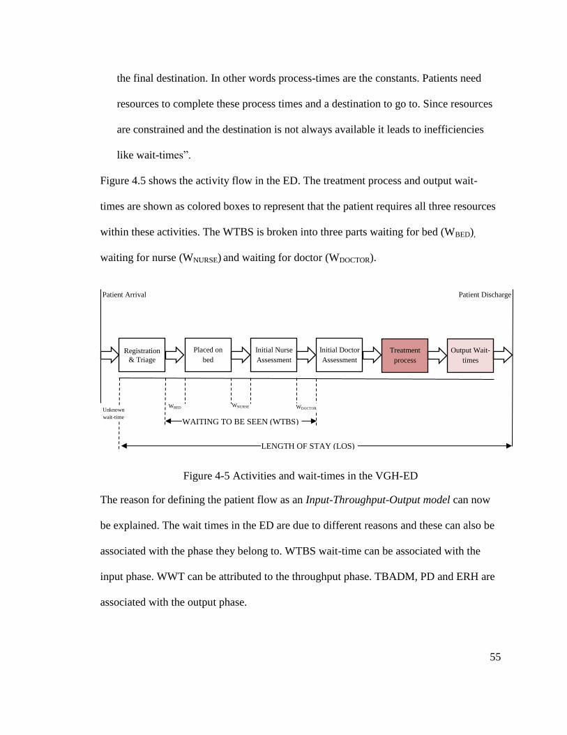
55
the final destination. In other words process-times are the constants. Patients need
resources to complete these process times and a destination to go to. Since resources
are constrained and the destination is not always available it leads to inefficiencies
like wait-times”.
Figure 4.5 shows the activity flow in the ED. The treatment process and output wait-
times are shown as colored boxes to represent that the patient requires all three resources
within these activities. The WTBS is broken into three parts waiting for bed (WBED),
waiting for nurse (WNURSE) and waiting for doctor (WDOCTOR).
Figure 4-5 Activities and wait-times in the VGH-ED
The reason for defining the patient flow as an Input-Throughput-Output model can now
be explained. The wait times in the ED are due to different reasons and these can also be
associated with the phase they belong to. WTBS wait-time can be associated with the
input phase. WWT can be attributed to the throughput phase. TBADM, PD and ERH are
associated with the output phase.
Registration
& Triage
Placed on
bed
Initial Nurse
Assessment
Initial Doctor
Assessment Treatment
process Output Wait-
times
WBED WNURSE WDOCTOR
WAITING TO BE SEEN (WTBS)
Unknown
wait-time
Patient Arrival
Patient Discharge
LENGTH OF STAY (LOS)

56
4.3.1. Prima-facie solution
The wait-times belonging to different phases are co-related. To reduce WTBS, direct and
indirect causes that effect WTBS should be understood.
The direct solution to reduce the WBED, WNURSE and WDOCTOR times is to add more of
these resources that cause this wait-time. Such a scenario, where resources are increased,
falls under the category of variable change scenarios.
The indirect solution is to free up existing resources from the throughput and output
phase so that they can be re-located to the input phase. This re-location can be done either
by finding ways to reduce output wait-times; causes of which lie outside of the ED or by
distributing resources more evenly between input and throughput phases. Either of these
scenarios will fall under the category of process change scenarios.
As argued in Chapter 2 (Section 2.4), variable change scenarios tend to be of a permanent
nature. Hence in this research, the aim will be to reduce WTBS, without increasing LOS
and without adding more resources.
Using the flowcharts (4.1, 4.2 and 4.3) as a conceptual model, simulation model logic is
developed in Chapter 6. However before the model is built data need to be collected and
analyzed which is discussed in Chapter 5.

57
5.Data collection for VGH-EDsim model
This chapter focuses on data collection from ED and how the data can be transformed for
using in the VGH-ED simulation model (VGH-EDsim model). This chapter has 2
sections dedicated to each of these aspects.
5.1. Data collection for VGH-EDsim model
The ED consists of several resources such as beds, nurses doctors etc. This data is
collected directly from visiting the ED and is given in Table 5.1.
Table 5-1 ED resource data
Beds
Monitor area 15 Monitored beds
Treatment area 4 Non-monitored beds
Minor treatment area 5 Non-monitored beds
Resuscitation area 2 Highly equipped monitored beds
Waiting areas
Main waiting area 35 chairs (including 8 orange chairs for patients waiting
for registration
Minor treatment waiting area 15 chairs
Nurses
Monitor area 4 nurses
Treatment area 1 nurse
Minor treatment area 1 nurse
Doctors
VGH-ED 2 Doctors during day 1 at night

58
Two methods were used to collect patient data for the VGH-EDsim model; historical data
collection and management estimates [9]. A large number of historical data were
provided by the hospital authorities, which comes through the Emergency Department
Information System (EDIS). Patient identity was deliberately left out to protect their
privacy. Some data that were not provided were collected while shadowing staff in the
ED and by using estimates by ED management.
Three months of historical data were provided through the Emergency Department
Information System (EDIS system) for 7883 patients. The data were provided in the form
of an excel sheet. These data include arrival time data, entry and exit time stamps from
various locations, start and end times of different statuses, start and end times of various
processes such as registration, triage, and basic patient information like age and CTAS
score.
The amount of time that a nurse or a doctor spends with a patient in the treatment phase is
not recorded in the EDIS data. Therefore the data have to be collected through
managerial estimates.
Not all collected data were used to build the model. Instead they were broken down into
two groups. The first group is called as model-building data and it comprises of the data
from the first two months of the total EDIS data. These data are used to build the model.
The second set is called as model-validation data (also mentioned as real ED data) for the
model validation. This technique of breaking down the data sets into two parts is known
as historical data validation technique [13]. More about validation is discussed in
Chapter 6. The model- building data comprise of almost 5200 patient entries for
generating credible probabilities and distributions.

59
5.2. Transforming VGH-ED data into model input data
The historical data available were in the form of absolute arrival times, time stamps and
location stamps. However the simulation model requires data in a different format. A
simulation model is built using constant values and values that vary over a range of a
probability. The constant values are the deterministic data such as number of resources,
capacity of waiting-rooms etc. as discussed in VGH-ED structure section (Section 4.1)
[9]. The probabilistic data are the ones that vary with a probability range [9]. Arrival-
times, process times, patient attributes such as age, CTAS score and treatment location
are examples of probabilistic data.
Probabilistic data can be further broken down into two kinds; discrete and continuous
data [9]. Examples of discrete data in the case of ED are age, CTAS score and treatment
location. These variables can only take limited number of discrete and integral values.
Such values are generated using a percentage table. Continuous data on the other hand
are required for those variables that can take any positive value. Such data are fit onto
distributions. Inter-arrival times and process-times in the ED are a prime example of
continuous data.
Three sets of probabilistic data were needed for building the VGH-EDsim model: arrival
data, patient attribute data and process-time data. While the first and third are forms of
continuous data, patient attributes are discrete.
Before discussing the methodology to generate these data, a few basic things need to be
stated. Distributions in this research were generated using a software called ExpertFit
[51] which is available as a separate software and is also a part of the Flexsim software

60
package. The main advantage of ExpertFit is that it can automatically compare up to 40
distributions with a data set and give automated-fitting analysis to the user for the closest
possible distribution function and its parameters. It also tells whether the fit of this
distribution is good, moderate or bad based on several goodness-of-fit tests. A goodness-
of-fit test compares a theoretical distribution with observed data and if the difference
between the observed data and the corresponding theoretical distribution is small, then it
may be stated with some level of certainty that the observed data could have come from a
set of data with the same parameters as the theoretical distribution [9]. Only distributions
with good or moderate fits were chosen for the VGH-EDsim model. Wherever the mean
of the data is taken as a measure of central tendency, normality tests were conducted in a
software from IBM called SPSS [52].
We can now look into the three sub-sections dedicated to different probabilistic data sets.
Some managerial estimates regarding unknown process times were also collected.
However since there is no methodology used to determine them, they will simply be
stated while discussing the simulation model in Chapter 6.
5.2.1. Arrival data
Arrival distributions are one of the most significant data that are required to build a
simulation model for an ED. Since the model-building data set is very large, it needs to
be broken down into sub-sets since large data sets are usually combinations of different
distributions [9]. Therefore the arrival distributions are generated separately for walk-in
arrivals and ambulance arrivals. In this section generation of walk-in arrival distributions

61
has been discussed. The same methodology was used to generate arrival distributions for
ambulance patients.
The historical EDIS data has absolute arrival times, whereas a distribution function can
only fit onto inter-arrival times; i.e. time interval between the arrivals of two consecutive
patients. There are two ways to convert the data into inter-arrival time distributions;
direct and in-direct.
In the direct method, inter-arrival times were calculated for all patient entries in the
model-building data set. This is done by subtracting the absolute arrival times of two
consecutive patients. However the inter-arrival times generated were very random and no
distribution with a good fit could be found.
To model this kind of erratic arrival behavior, an indirect method has been used. Rather
than fitting the actual inter-arrival times onto distributions, the data is interpreted in terms
of patient arrival rate.
To identify an arrival-rate, the walk-in data need to be further organized and condensed.
The model-building data set had a single column of absolute arrival time entries for about
3800 walk-in patients over 61 days. These data were broken down into an hour of day by
week day table in 3 steps.
Table 5-2 Hour by Day table (number of patients in an hour of a day)
Hours
of Day
from 1
to 24
61 Days (1st May-30th June)
Day 1 Day 2 Day 3 … … Day 61
Hour 1 3 2 5
2
Hour 2 1 1 1
1
Hour 3 0 0 1
2
…
Hour 24 2 1 2 2

62
In step 1, the column data were transformed into a table with 24 rows and 61 columns.
This table can be called as an hour by day number table, as each row represented the 24
hours in a day and each column represented one of the 61 days. A snapshot of this table is
shown in Table 5.2. Each element of the table equals to the number of patients arriving in
hour h (row) of day d (column). Thus more than 3800 (walk-in patients) entries were
redistributed into 1464 (61*24) entries of patients arriving per hour.
Table 5-3 Hour by Weekday occurrence table (number of patients in an hour of a day)
In step 2, the hour by day table was broken into 7 different tables based on 7 days of the
week and can be called as hour by weekday occurrence tables. In the data sample each
day of week occurs 9 times with the exception of Friday and Saturday which occurred 8
times. This step divides the total data (1464 entries) into seven smaller tables each having
approximately 200 entries. A snapshot of such a table for Sunday is shown in Table 5.3.
Table 5-4 Hour by Weekday table (average number of patients in an hour of a weekday)
Hours
of Day
from
1 to 24
Number of times a Sunday occurs
Day 1 Day 8 Day 15 … Day 50 Day 57
Hour 1 3 3 2
3 2
Hour 2 1 2 0
3 2
Hour 3 0 2 1
1 1
…
Hour 24 2 3 2 0 1
Hours of Day from 1 to 24
All days in the week
Sunday Monday Tuesday Wednesday Thursday Friday Saturday
Hour 1 1.69 2.08 1.31 1.92 1.23 1.15 1.62
Hour 2 1.62 1.23 1.15 1.08 1.15 1.23 1.54
Hour 24
2 2.77 2.46 2.08 2.54 1.85 1.92

63
In the 3rd
step average number of patients coming in given hour for a given weekday is
calculated. For example values in all rows of Table 5.3 were averaged and a single
column table for Sunday was obtained. This was repeated for all 7 hour by weekday
occurrence tables. The 7 column tables were then merged back into one table as shown in
hour by weekday table (Table 5.4).
Each of the value in Table 5.4 represents average number of patients arriving in a given
hour of the day. These values are used as denominators with numerators as 60 minutes.
This gives us the average inter-arrival time in a given hour of a given weekday as shown
in Table 5.5.
Table 5-5 Inter-arrival time table (in minutes)
This data can be used to identify patient arrival patterns. The values of Table 5.4 are
averaged across columns and turned into a single row data. This row is used to make a
line graph with error bars as shown in Figure 5.1. Evidently the error is very small and
Hours of Day from 1 to 24
All days in the week
Sunday Monday Tuesday Wednesday Thursday Friday Saturday
Hour 1 35.5 28.85 45.8 31.25 48.78 52.17 37.04
Hour 2 37.04 48.78 52.17 55.56 52.17 48.78 38.96
Hour 3 55.56 48.78 60 55.56 96.77 77.92 38.96
…
Hour 24
30 21.66 24.39 28.85 23.62 32.43 31.25
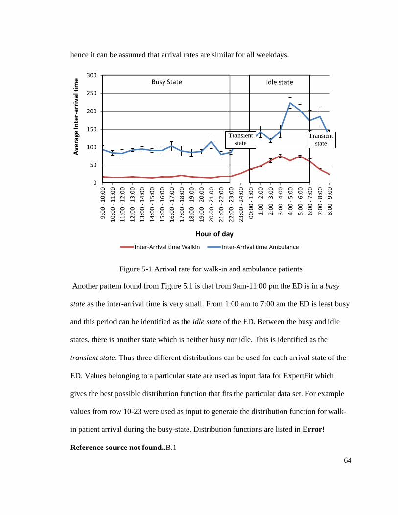
64
hence it can be assumed that arrival rates are similar for all weekdays.
Figure 5-1 Arrival rate for walk-in and ambulance patients
Another pattern found from Figure 5.1 is that from 9am-11:00 pm the ED is in a busy
state as the inter-arrival time is very small. From 1:00 am to 7:00 am the ED is least busy
and this period can be identified as the idle state of the ED. Between the busy and idle
states, there is another state which is neither busy nor idle. This is identified as the
transient state. Thus three different distributions can be used for each arrival state of the
ED. Values belonging to a particular state are used as input data for ExpertFit which
gives the best possible distribution function that fits the particular data set. For example
values from row 10-23 were used as input to generate the distribution function for walk-
in patient arrival during the busy-state. Distribution functions are listed in Error!
Reference source not found..B.1
0
50
100
150
200
250
300
9:0
0 -
10
:00
10
:00
- 1
1:0
0
11
:00
- 1
2:0
0
12
:00
- 1
3:0
0
13
:00
- 1
4:0
0
14
:00
- 1
5:0
0
15
:00
- 1
6:0
0
16
:00
- 1
7:0
0
17
:00
- 1
8:0
0
18
:00
- 1
9:0
0
19
:00
- 2
0:0
0
20
:00
- 2
1:0
0
21
:00
- 2
2:0
0
22
:00
- 2
3:0
0
23
:00
- 2
4:0
0
00
:00
- 1
:00
1:0
0 -
2:0
0
2:0
0 -
3:0
0
3:0
0 -
4:0
0
4:0
0 -
5:0
0
5:0
0 -
6:0
0
6:0
0 -
7:0
0
7:0
0 -
8:0
0
8:0
0 -
9:0
0
Ave
rage
Inte
r-ar
riva
l tim
e
Hour of day
Inter-Arrival time Walkin Inter-Arrival time Ambulance
Busy State Idle state
Transient
state Transient
state

65
5.2.2. Patient attribute data
Patients journey, the path he/she takes inside the ED and the time the patient spends in
the ED is dependent largely upon the patient’s attributes such as his/her illness, criticality
of illness, age and social background. These attributes need to be replicated in the
simulation model in order to represent reality. The patient attributes that are replicated in
the VGH-EDsim model are the patient’s arrival mode, age, CTAS score, treatment
location and patient’s discharge disposition (admit or non-admit). Since all of these
attributes can only take a few discrete integral (considering age as an integer) values,
these data have been categorized as discrete probabilistic data.
Patient’s arrival mode 5.2.2.1.
This attribute is generated with the arrival of the patient in the model and is dependent
upon the source which generates the patient. Patient’s arrival mode forms the basis of all
future probability generations.
Patient age data 5.2.2.2.
The age of the patient is the first attribute that is generated using a probability table. In
real world scenario the patient’s age could be anywhere between 0-120 years (for all
practical purposes). However to model an attribute with such large number of possible
values is neither feasible nor required. It is not feasible because if we divide the data into
120 possible sub-groups the sample size in each group would become insufficient to
generate an accurate probability. It is also not required because if future probabilities
have to be based on age, they cannot be based on 120 different values and thus the values
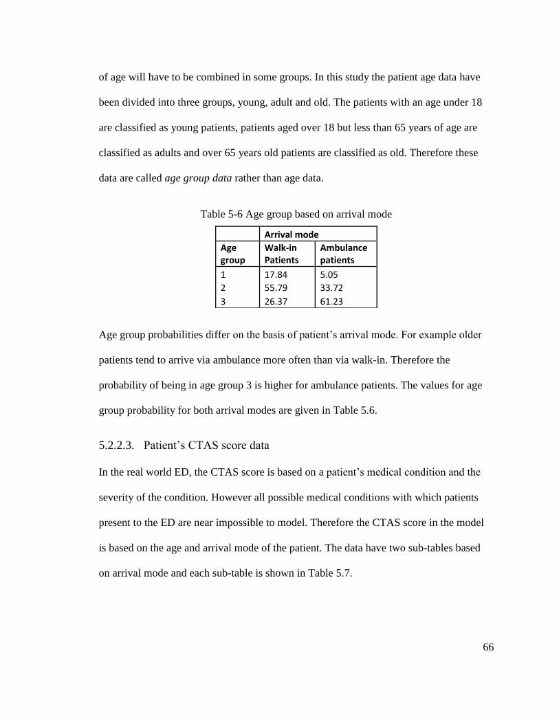
66
of age will have to be combined in some groups. In this study the patient age data have
been divided into three groups, young, adult and old. The patients with an age under 18
are classified as young patients, patients aged over 18 but less than 65 years of age are
classified as adults and over 65 years old patients are classified as old. Therefore these
data are called age group data rather than age data.
Table 5-6 Age group based on arrival mode
Age group probabilities differ on the basis of patient’s arrival mode. For example older
patients tend to arrive via ambulance more often than via walk-in. Therefore the
probability of being in age group 3 is higher for ambulance patients. The values for age
group probability for both arrival modes are given in Table 5.6.
Patient’s CTAS score data 5.2.2.3.
In the real world ED, the CTAS score is based on a patient’s medical condition and the
severity of the condition. However all possible medical conditions with which patients
present to the ED are near impossible to model. Therefore the CTAS score in the model
is based on the age and arrival mode of the patient. The data have two sub-tables based
on arrival mode and each sub-table is shown in Table 5.7.
Arrival mode
Age group
Walk-in Patients
Ambulance patients
1 17.84 5.05
2 55.79 33.72
3 26.37 61.23

67
Table 5-7 Percentages of CTAS based on arrival mode and age
Patient’s treatment location 5.2.2.4.
Patient’s treatment location is based on patient’s medical condition and its severity
(CTAS). To replicate this in the model, the treatment location is based on the CTAS
score of the patient. For example a patient with a low CTAS score of 2 or 3 is more likely
to need a monitor bed and patients with CTAS score 4 or 5 are more likely to require
non-treatment beds in treatment or minor treatment area.
However generating treatment location data is not that simple. In practice, patients are
often transferred from one bed to another during their treatment as per the need of the
hour. This behavior is very difficult to model as there can be many possible reasons for
bed transfers. Therefore the bed-transfers are ignored while building the simulation
model.
The original data file had timestamps for different locations which helped generate the
amount of time spent at a particular type of bed. The assumption made for this research is
that if the patient spent time in more than one bed areas, the area where he/she spent the
maximum time is chosen as the treatment location for model purposes. Based on this
assumption 5 probability tables were generated for 5 CTAS scores each having 4 possible
Arrivals via Walk-ins
Arrivals via Ambulance
Age
group 1
Age
group 2
Age
group 3
Age
group 1
Age
group 2
Age
group 3
CTAS 1 0.61 0.92 2.19
CTAS 1 0 5.87 4.57
CTAS 2 5.41 10.67 11.1
CTAS 2 17.57 18.62 18.51
CTAS 3 21.31 29.54 36.98
CTAS 3 31.08 37.25 38.57
CTAS 4 55.63 44.85 38.28
CTAS 4 47.3 35.63 35.23
CTAS 5 17.03 14.02 11.46
CTAS 5 4.05 2.63 3.12

68
treatment locations: Monitor, Resus, Treatment and Minor treatment area. These data are
shown in Table 5.8.
Table 5-8 Treatment location percentages based on CTAS
Patient’s discharge disposition data 5.2.2.5.
Patient discharge disposition is a binary decision. A patient either gets admitted and if not
then he/she is discharged back to the community. If a patient needs to be admitted, he/she
will almost always go through the TBADM wait-time. But in the case of non-admits only
some patients go through PD wait-time while others may go through an ERH wait-time.
No patient goes through more than one wait-time.
Three probabilities are needed to represent this scenario. First probability can be defined
as patient’s admission probability. If a patient turns out to be a non-admit then there is a
second probability of whether the patient will go through PD wait-time. The third
probability is whether the remaining of the non-admit patients that may go through an
ERH process.
All of these probabilities were found to be dependent on age. Older patients have a higher
chance of going through ERH and also have a higher admission rates than younger
patients. Even in the case of non-admitted patients older patients go through PD wait-
time more often than younger patients. The probability data are given in Table 5.9.
CTAS 1 CTAS 2 CTAS 3 CTAS 4 CTAS 5
Resuscitation 20.41 1.88 1.59 0.91 0.86
Monitor 63.27 70.54 48.18 24.87 9.63
Treatment 9.18 14.455 26.42 37.96 43.96
MTA 7.14 13.125 23.82 36.26 45.56

69
Table 5-9 Discharge disposition probability percentages based on Age
5.2.3. Process time data
Process times can take any value and are not limited to a few discrete values. Therefore
process time data fall under the category of continuous probabilistic data. The reason for
discussing process time data after patient attribute data is because process times are based
on patient attributes.
There are four major process time data that could be abstracted from the EDIS data.
These are treatment in progress times (TIP), pending discharge times (PD), to be
admitted times (TBADM) and Emergency room hold times (ERH). In real ED the last
three are wait-times but since the VGH-EDsim model has not been linked to the external
world, the model cannot generate these wait-times. However to model their effect on the
ED, these have been modeled as process-times.
The length of TIP status can be calculated directly from the model-building data as time
stamps for beginning and end of TIP are given. However the whole data should not be
fitted onto a single distribution as TIP process time depends largely on the patient
condition. The distributions are given in Error! Reference source not found.. The
amount of time a nurse or a doctor is utilized by the patient is calculated by dividing TIP
time by nurse factor and doctor factor, which is assumed to be 4 and 20, respectively.
TBADM PD ERH
Age group 1 0.66
Age group 1 19.52
Age group 1 1.07
Age group 2 3.8
Age group 2 25.82
Age group 2 6.04
Age group 3 17.45 Age group 3 29.85 Age group 3 23.44

70
Since a patient’s medical condition cannot be modeled, the patient treatment location and
arrival mode are chosen as the best possible estimates of a patient’s health.
The length of the TBADM and PD time does not depend upon age as these wait-times are
dependent on the blockage in the external system rather than condition of the patient.
ERH process times however were seen to be a function of age. It can be inferred that
medical conditions of older patients are generally more complex and thus they have to be
observed for a longer period of time. The output-phase process time distributions are
given in Error! Reference source not found..

71
6. The Simulation model
This chapter is completely dedicated to the VGH-EDsim model. It is divided into three
sections. In the first section, FlexSim, the software used to build the model, is briefly
introduced. The second section explains the model building methodology. The third
section details the different stages in which the VGH-EDsim model was built.
6.1. Introduction to Flexsim 3D simulation software
There are three types of objects in the FlexSim’s object library, namely the flowitems,
fixed resources and task-executers. Flowitems represent the entity that flows through the
system. FlexSim allows the user to choose different kinds of items from an existing
flowitem bin or to create a custom flow-item. Processors, multi-processors, queues,
sources, sink and dispatchers all fall under the category of fixed resources, since the
quantity is fixed in a simulation run. Task-executers represent human or robotic
operators/transporters that can process an item at a processing station and/or move items
from one fixed-resource to another. Fixed resources and task-executers are connected to
each other through their ports. The ports are of three kinds; input ports, center ports and
output ports. Fixed resources such as processors and queues receive items from input

72
ports and release them through output ports. Additional resources, such as task-executers
required by processors and queues for various activities are connected via a center port.
Every object in FlexSim library can have attributes which differentiates it from others of
its kind. Fixed-resources have attributes such as process times and capacity. Flowitems
have an additional attribute called itemtype which can take a positive integral value. The
user can decide these attributes and their values and store them in labels. Labels can take
either a string or number value depending upon the attribute the user wants to decide.
Since FlexSim is a simulation software system, the state of the model changes at default
events. In the software package these events are also called as triggers. The state of the
system changes on these triggers.
Since fixed-resources are of many kinds, they can have different kinds of triggers. As a
default for every fixed resource, there is an on entry, on exit, on message and an on flow
trigger to represent Discrete-events. A modeller can write a program inside any of these
triggers as per the simulation logic. The modeller can use attributes of flowitems and
fixed resources stored in labels to build logic for individual code.
Apart from these, FlexSim also provides ways where objects of the system can
communicate. Any object in FlexSim can send coded messages to other objects. Every
message has 3 parameters which can take any value therefore there is an infinite number
of differently coded messages that can be sent. FlexSim also lives up to its promise of
flexibility as it also allows a user to create custom events. An object in FlexSim can also
send a delayed message to another object. While the command itself runs inside a default
event, it can create an event for future and the default event acts as a reference point.
Another way to create a custom event is to create a user event. The first user event time
73
and the subsequent intervals can be defined. The communication feature and the user
event feature are essentially used for agent-based modeling and their usage will be
discussed in Chapter 7.
6.2. Steps to build a DES model for VGH-ED
When sufficient knowledge about the patient flow has been achieved (validated
conceptual-model), model input data can be abstracted from VGH-ED data. In this
section, the steps required to transform this knowledge into a validated simulation model
to conduct experimentation are discussed.
Even the simplest simulation model requires a considerable amount of programming,
therefore one should avoid building the whole model without debugging [9]. It could be
extremely difficult to make such a model error free. Therefore to build the VGH-EDsim
model, a divide-and-conquer approach was used [9]. Under this approach the model is
built in stages and in each stage a few details are added and the model is checked for
errors. The actual stages of VGH-EDsim model building have been discussed in the last
section of this chapter.
In every stage/iteration, 5 basic steps are followed. The process of model building ends
when all details have been successfully modeled. The first step in this methodology is to
decide the level of detail to be included in that iteration. The second step is to decide the
simulation model logic to model the chosen level of detail and the third step is to code a
simulation model that runs that logic. The model is verified and validated in steps 4 and
5. Verification is the process by which it is determined if the model works as intended
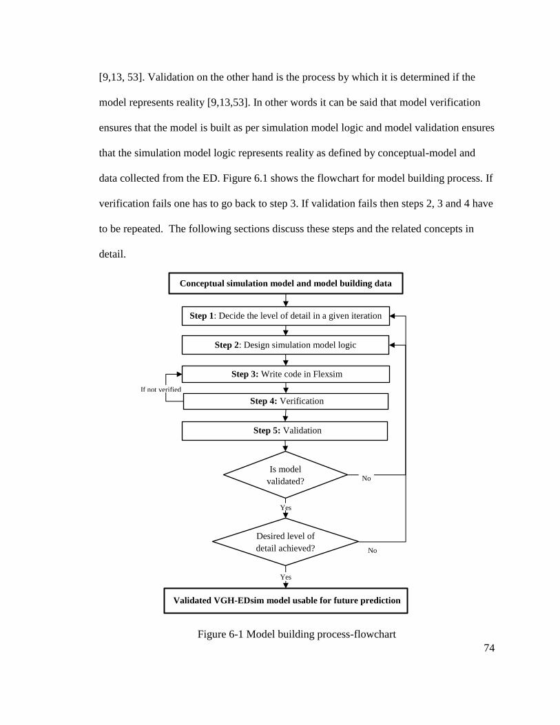
74
[9,13, 53]. Validation on the other hand is the process by which it is determined if the
model represents reality [9,13,53]. In other words it can be said that model verification
ensures that the model is built as per simulation model logic and model validation ensures
that the simulation model logic represents reality as defined by conceptual-model and
data collected from the ED. Figure 6.1 shows the flowchart for model building process. If
verification fails one has to go back to step 3. If validation fails then steps 2, 3 and 4 have
to be repeated. The following sections discuss these steps and the related concepts in
detail.
Figure 6-1 Model building process-flowchart
Step 1: Decide the level of detail in a given iteration
Step 2: Design simulation model logic
Step 4: Verification
Step 5: Validation
Conceptual simulation model and model building data
Step 3: Write code in Flexsim
Validated VGH-EDsim model usable for future prediction
If not verified
No Is model
validated?
Desired level of
detail achieved? No
Yes
Yes

75
6.2.1. Step1: Deciding the scope of the model
As mentioned earlier, a divide and conquer approach is needed to build the VGH-EDsim
model. Different aspects of the model are coded in different iterations. The details are
discussed in Section 6.3.
The scope of the VGH-EDsim model includes:
1.) Output phase wait-times (ERH, TBADM and PD) built as individual process times.
2.) The treatment times captured from the data with smaller process times to capture the
cyclic nature of the treatment process.
3.) The resources (bed, nurse and doctor), their behaviors and processes in the input
phase modeled to generate input waiting-time (WTBS) and total LOS as close to
reality as possible.
6.2.2. Step 2: Designing simulation model logic
To transform the conceptual-model and model input data into a simulation model,
simulation model logic is required. The simulation model is nothing but simulation model
logic running in a simulation software package. For ease of explanation the simulation
model logic is also presented in an input-throughput-output phase. As FlexSim is
primarily a manufacturing-software, the objects in the object library do not relate to
patients and resources of the ED. Therefore in the VGH-EDsim model, the processors are
used as registration and triage desks, multiprocessors as beds, sources are used to create
patients, sink is used to discharge patients and queues represent waiting-rooms. Figure
6.2 show a snapshot of the simulation model. To represent the four bed areas, the VGH-

76
EDsim model has 4 bed clusters with the same names as the bed areas. Each cluster has a
number of multiprocessors and a queue.
Figure 6-2 Snapshot of VGH-EDsim model
Input phase of simulation model logic 6.2.2.1.
The simulation logic for the input phase is given in Figure 6.3. Two sources create
patients using the arrival distributions. From there the patient goes to the first queue
called waiting for registration where he/she waits for the registration processor to
become available. The entry trigger of registration processor has code written on it to
record patient’s arrival time and decide patient’s age. After registration the patient goes to
waiting for triage queue where the patient waits for a triage processor. The patient’s
CTAS is decided on entry trigger of the triage processor based on the age and arrival
mode. Patient’s prospective treatment location is decided based on CTAS score of the
patient. After triage the patient is sent to one of the 4 waiting for bed queues based on the
treatment location. These queues distribute the patients randomly amongst available beds
in that bed area. This step is called the bed-allotment decision.

77
Figure 6-3 Input phase of simulation model logic
Source 2 Ambulance
Patients
Waiting for
Registration
Waiting for
Triage
Triage 1 Triage 2
Waiting for
Resus Bed
Source 1
Walk-in
Patients
On Inter-arrival time trigger
<Enter arrival distributions>
Registration
Process
On Entry trigger <Record arrival time>
<Set age based on arrival mode>
On Entry trigger <Set CTAS based on arrival mode
and age> <Set treatment location on the
basis of CTAS>
Waiting for
Monitor Bed Waiting for
Treatment Bed Waiting for
MTA Bed
LEGEND
Processor
Action on triggers
Queue
Source
On Flow trigger
< Select 1 out of available
locations randomly>
On Flow trigger < Select based on treatment
location decision >
Bed 1
Bed 2
Bed 3
Bed 4
Bed 16
Bed 20
Bed 17
Bed 21
Bed 22
Bed Area Bed 16 Bed 25

78
Throughput phase of simulation model logic 6.2.2.2.
As soon as the patient is able to get a bed as his/her pre-decided treatment location, the
throughput phase on patient’s journey begins. The simulation logic for the throughput
phase is shown in Figure 6.4. The multiprocessor that represents the bed performs many
sub-processes. On the entry trigger of the multi-processor, the TIP time is generated and
total nurse and total doctor times are decided by dividing the TIP by nurse and doctor
factors. The logic is as follows:
Calculate TIP based on arrival mode, age and treatment location;
Total nurse time = TIP/Nurse factor;
Total doctor time = TIP/Doctor factor; // where nurse factor = 4, doctor factor = 20
The first sub- process is called initial nurse assessment in which the multi-processor calls
the nurse resource followed by initial doctor assessment where the doctor resource is
called by the multi-processor. Process times for these two processes are fixed and every
patient goes through them only once. To represent the various processes such as lab-tests,
specialist consults etc. a sub-process called black-box process 1 is modeled, after the
initial doctor assessment. A process can be modeled as a black-box if its actual working
is unknown and only the input and output characteristics of the process are of concern
[54]. The duration for this process is 20 minutes of TIP time whichever is less. The
multiprocessor does not need to call any other resource during this process.

79
Figure 6-4 Throughput phase of simulation model logic
BED
On Entry trigger <Set Total TIP time based on
treatment location and arrival mode>
<Set Total Nurse Time = TIP/4>
<Set Total Doctor Time = TIP/20>
Initial Nurse Assessment = 10
minutes
Else 0 minutes
Record WTBS time Initial Doctor Assessment = 10
minutes, Else 0 minutes
Black Box process 1 = 20
minutes
Else 0 minutes
If Total Nurse Time >20 minutes
Nurse Assessment Time = 20
minutes
Else = Total Nurse Time
On Process Finish Trigger <Update Nurse time = Total Nurse
Time –Nurse Assessment Time>
<Update TIP time = TIP – Nurse
Assessment time>
If Total Doctor Time >20
minutes Doctor Assessment Time = 20
minutes
Else if Nurse Time = 0 Doctor Assessment Time =
Total Doctor Time
Else Doctor Assessment Time =
0 minutes
If TIP time > 20 minutes Black Box process 1 = 20
minutes Else = TIP time
On Process Finish Trigger <Update Doctor time = Total
Doctor Time –Doctor Assessment
Time>
<Update TIP time = TIP – Doctor
Assessment time>
If TIP
time = 0 No
LEGEND
On Pick trigger <Call Nurse>
On Pick trigger <Call Doctor>
On Pick trigger <Call Doctor>
On Pick trigger <Call Nurse>
Action on triggers
Multi-Processor
Sub-processes
Yes, towards
output phase

80
After this sub-process the cyclic nature of the treatment process begins. Followed by the
black box process 1, is the nurse procedure process. This represents the process of the
ED where the nurse processes doctor’s orders and monitors the patient. The time of this
monitoring is 10 minutes or total nurse time whichever is less. After this the nurse calls
the doctor and the duration of the doctor reassessment process is given by the following
logic:
If total doctor time >10 minutes, duration = 10 minutes;
If total doctor time < 10 minutes, check if nurse time = 0;
If nurse time = 0, duration = doctor time, else duration = 0;
The reason behind this logic is that the final doctor process should only occur if all nurse
time has been exhausted. In the ED the doctor takes the final decision and that is
represented by this logic. Another process called Black box 2 is followed by the doctor
reassessment which is exactly the same as black box 1 process. If all the TIP is exhausted
after this process the patient moves to output phase, else the patient goes back to the
nurse procedure process.
Output Phase of simulation logic 6.2.2.3.
The output phase happens on a separate multi-processor connected to the primary
multiprocessor where treatment took place, however the main multi-processor does not
except new patients until the current patient has finished the output phase of his/her
journey.

81
Figure 6-5 Output phase of simulation model logic
On the entry-trigger of the output multi-processor, the decision whether the patient goes
through any one of the TBADM, ERH or PD processes is made and the process times are
also determined. The order of sub-processes is shown in Figure 6.5. The TBADM and the
ERH processes require nurse and doctor resources. The nurse and doctor times are
decided as factors of these processes (See Table 5.9). The output phase is not modeled in
OUTPUT BED
On Entry trigger <Decide whether patient is an admit or
non-admit>
<If admit decide TBADM time>
<If non-admit decide if ERH?>
<<If yes decide ERH time?>>
<<If no decide if PD?>>
<<<If yes decide PD time>>>
<Set TBADM time>
<Set ERH time>
<Set PD time>
<Set Nurse time =ERH or TBADM/6>
<Set Doctor time = ERH or TBADM/40>
ERH_nurse process = ERH
time/2
ERH_doctor process = ERH
time/2
TBADM_nurse process =
TBADM time/2
TBADM_doctor process =
TBADM time/2
PD process = PD time
On Pick trigger <Call Nurse if TBADM> 0>
<<if yes utilize nurse for
Nurse time>>
On Pick trigger <Call Doctor if TBADM> 0>
<<if yes utilize doctor for
Doctor time>>
On Pick trigger <Call Nurse if ERH> 0> <<if yes utilize nurse for
Nurse time>>
On Pick trigger <Call Doctor if ERH> 0> <<if yes utilize doctor for
Doctor time>>
LEGEND
Action on triggers
Multi-Processor
Sub-processes
DISCHARGE

82
a cyclic order because the utilization of nurses and doctors is far less compared to the
treatment process.
Reduction factor for TIP 6.2.2.4.
A lot of sub-processes shown in Figures 6.4 and 6.5 require a nurse or a doctor resource.
Since these resources are scarce there is a wait-time between these sub-processes. In
Figure 5.6 the activity flow within the treatment process is given. The activities are
shown in boxes and wait-times are represented by arrows. It clearly represents that the
actual activity time is less than the total TIP-time. The total TIP can be broken into:
Figure 6-6 Activity flow within treatment phase
The data collected from the VGH-ED do not give details about the waiting time with-in
the treatment phase. Moreover there is no credible way to determine the actual activity
time and the wait-time. Therefore a method was needed to extract the actual TIP time
from the total TIP time. It is therefore assumed that actual activity time is a fraction of the
total TIP time, i.e. the total TIP can also be written as:
Initial nurse
assessment
Initial doctor
assessment
Black box
process 1
Nurse
procedure Doctor
reassessment Black-process
2
WNURSE
TREATMENT IN PROGRESS
Patient
placed on
bed If TIP
= 0?
Ou
tput-
ph
ase
N
WDOCTOR
WNURSE
WDOCTOR

83
Where the value of the reduction factor = .75 (found out using hit and trial method)
6.2.3. Step 3: Writing the simulation model logic in FlexSim
The model code is a set of several codes written on different triggers in the model. It is
these set of codes that guide the flowitem through the model. To write a basic program in
FlexSim one has to learn a few basic concepts of FlexSim.
The model built in FlexSim has a tree structure where every fixed-resource and task-
executer exists represents a node. The items are also temporary nodes that flow between
the fixed-resource nodes. Each node has certain attributes. For example all fixed
resources can have labels on them which represent their attributes.
FlexSim uses its own coding language called Flexscript which consists of about 700
commands. A command can take 3 different types and combinations of inputs; node,
number, and string. Depending upon the nature and purpose of the command it could
return either a node, or a number or a string. An example of a command that takes node
and string as input and gives a number as output is:
getlabelnum(current,”Bed type”);
getlabelnum(item,”Patient number”);
In this example the command getlabelnum is executed upon node current (fixed-
resource) for fetching the value of the label named Bed type (attribute). The value of this
label is the form of a number. It can be said that by default, the node named current is the
fixed-resource where this code is being executed. In the second line the same command is

84
being executed upon node named item a term used for the flowitem currently at the fixed-
resource called current.
Flexscript being similar to C++ has if, else, for and while commands, for a case where the
code needs to be run based on some condition. For example
if( getlabelnum(item,”Patient number”) == 4)
{
return 4;
}
else return 0;
It is noticeable how a conditional logic can be developed. For creating the condition the
operation “==” is used for comparing a number variable with a number constant. So if
this comparison is true the getlabel command returns a number which is equal to 4 then
the code inside the curled brackets is executed otherwise the code written after the else
command is executed. The return command is used before declaring values for triggers
that are supposed to generate values. For example an on process time trigger is supposed
to generate a value for process time therefore a return command is used to do so.
The more complicated codes are usually tested on a dummy model before implementing
them to the full model. Right after a code is written the next process is verification.
6.2.4. Step 4: Verification of the model
The verification is the process of verifying the code of the model. Every iteration of
model building needs to be verified. Since the model in each iteration is built by many
smaller codes, each of these codes can be built into a dummy model which can be
verified separately. Verification is usually done to identify two types of errors in a code;
syntax and logic.

85
Syntax can be a simple spelling mistake which the software captures very easily. FlexSim
has the capability to detect certain errors and it reports them under system console. The
most common of such errors is the one when the code is called upon/for something that
does not exist. Any such behavior is termed as an exception. Whenever an exception
occurs, FlexSim also gives the user some information about the exact time and source of
error. Once the source and cause of error is identified and understood the code is fixed.
Syntax errors are very easy to catch as the model automatically detects them.
Verification of syntax does not mean that the model logic is also verified. Sometimes a
code is written in a way that it works for a range of values but fails beyond that range.
Therefore a modeller needs to verify a code for a range of situations.
Model’s logic verification can be tricky as wrong logics are not as easily detectable as
wrong syntax is. To help the user, FlexSim has many inbuilt tools. FlexSim can generate
an event log in which every event, its time and the objects participated in that event are
listed. It is particularly helpful if the behavior of a particular fixed-resource such as a bed
or queue needs to be verified.
Sometimes if a user is not fully confident of the code written, FlexSim has a tool called
step debugging. The user can put a red dot on the left side of those lines of code where
the user wants to stop and verify the behavior. Once the model is stopped the user can
click on the step into button to stop the model at the next line of code. Thus instead of
trying to identify sources of error or abnormal behavior in a running model the user can
start and stop the model at chosen points. This feature has been particularly used to
verify the VGH-EDsim model.

86
Another technique, commonly used to verify a simulation model, is by generating a
variable/attribute output file in which data (wait-times, process times attributes etc.) for
each patient is recorded [9]. The modeller can then scan the output file for any anomalies.
6.2.5. Step 5: Validation of the model
While verification means to ‘build the model correctly’, validation means to ‘build the
correct model’ [9]. There are many possible ways to compare the simulation model with
the real system and the validation process is often based on the purpose of the model and
research goals [53]. For example if the need of the research is to build a more predictive
model, the technique used to validate it must also be foolproof.
Even in a given model certain parts of it are built in more detail than others (section
5.3.2) and the model validated for a particular purpose may not be validated for another
as there is no such thing as general validity [53]. For example in the VGH-EDsim model
the input and throughput phases of the model are built in more detail so they need to be
robustly validated but in other parts such as inter-arrival time and output phase wait-times
a lot of assumptions are made and thus these aspects should not be tested with the
strictest validation techniques.
As the goal of the research aims to predict improvements in WTBS and LOS, these two
are chosen as the main parameters for model validation and will be subjected to more
robust tests. Individual process times are used as secondary parameters for generating
more confidence for example TIP process time. Activities such as ERH, TBADM and PD
were added and a comparison was made between total output-phase wait-times from the
data and total output-phase process times from the model. As mentioned in Section 5.1,

87
the third month’s data called the model validation data are used as a basis to validate the
VGH-EDsim model
Model validation techniques: Subjective and Objective 6.2.5.1.
There are two techniques used for model validation; subjective and objective. The
subjective techniques are used to ensure that the model, at least on the surface, represents
reality [9]. One such technique is face validity where it is determined that the model’s
patient flow is in-line with the patient flow of the conceptual-model [9, 13]. Subjective
validation is often confused with model verification. However one should remember that
in verification the behavior of the code is tested and in validation the sequence of events
is tested against that of conceptual simulation model. The same tools used for verifying
the logic of the code such as event log and step debugger, can also be used to validate the
sequence of events of the model. This validation technique is also called as tracing where
behaviors of specific types of entities is analyzed [13]. If the sequence of events is found
to be incorrect the modeller may need to repeat the verification process or in some cases
may need to revisit the simulation model logic. Apart from sequence of processes the
modeller can also test special circumstances and check if the model is in line with the
conceptual-model.
Subjective assessments are necessary but are insufficient to validate a model on their own
[9]. To validate the model with greater precision an objective assessment, which is based
on some type of mathematical procedure, is required [13].
Objective techniques are used to compare data output from the model with collected data.
There are two types of objective techniques; qualitative and quantitative. Qualitative
88
analysis is a combination of subjective and objective assessments and is done to examine
if the magnitudes of the output behavior of the model are ‘reasonable’ [13]. For example
comparing average values for model and data is a qualitative analysis. Similarly
graphical analysis is another qualitative technique, as it is a combination of objective and
subjective analysis (visual inspection is always subjective). Quantitative analysis, on the
other hand, is completely objective and involves some kind of statistical test. The choice
of the statistical test is based on whether the data sets are normal or not.
In order to predict accurate WTBS and LOS, the most objective validation technique
should be followed, whereas for the remaining aspects of the model the validation
technique can be partially objective.
Collecting data from the model for validation 6.2.5.2.
In all stages and iterations of model building, validation is done objectively which
requires that model output data set is compared with the model validation data set (data
from the third month of EDIS data, 2701 patients). The procedure of collecting model
output data depends upon the system that is being modeled.
Simulation models can be of two types; terminating and non-terminating. Terminating
systems are the ones that run for a fixed period of time, such that the previous period has
no effect on the starting conditions of the next period. In contrast non-terminating
systems are those which run for a period of time but at the starting of a new period,
entities from the previous period may exist [9].
The VGH-ED is a 24 hours and 7 days facility. The ED virtually never stops and even if
it is studied for a particular period, the ED will have patients at the beginning of that

89
period. In non-terminating systems such as ED, initially the model is empty and therefore
the first few patients have very less wait-times and length of stay as all resources are
readily available. However after a while as the arrival rate remains faster than patient
discharge rates the model fills up. This filling up period is known as warm-up time and is
also known as transient state of the model. After the transient state is over and the model
is filled up, it is said to be in steady state.
The point where the transient state ends and steady state begins is usually different in
every model replication even if all other parameters are same. This point can be
calculated using a graph where time is plotted on x-axis and running average of WTBS is
plotted on y-axis. Running average of WTBS means the average value of all WTBS
values up to that point. For example for patient ‘Pn’ with WTBS as ‘W
n’ running average
of WTBS is be given by:
In this plot the user visually determines a steady state line, beyond which the slope of the
graph approaches to 0. The data on the right side of the chosen point can be used as a
pool to pick model output data. The same line can be chosen for all the other process
times. An example of a steady state analysis graph is shown in Figure 6.7.

90
Figure 6-7 Steady state analysis for a typical VGH-EDsim model run
As in most of the iterations (out of 10), after around 5000 patients the slope of the graph
stabilizes to approach zero, it is roughly chosen as a steady state line. To be on a safer
side, 2701 patient entries starting at patient number 5000 can be picked for the model
output data as shown in Figure 6-7.
In all stages of modeling where objective validation is made, the above mentioned
procedure has been followed to collect model output data.
6.3. Stages of building VGH-EDsim model
In this section, the actual stages of building of the VGH-EDsim model are discussed. The
simulation model has 3 main resources; beds, nurses and doctors. As mentioned before, a
0
100
200
300
400
500
600
700
800
Tim
e in
min
ute
s
Number of patients
WTBS LOS TIP
Steady state line

91
divide and conquer approach was followed to build the simulation model. The model was
built in 3 stages and staring with the bed resource, one resource was added in each stage.
In each stage two separate identical models were developed, called as VGH-ED data
model (or the data model) and VGH-ED distribution model (or the distribution model).
In Chapter 5, it was mentioned how data collected from the EDIS was first converted into
absolute arrival times and process times for individual patients. While this data were
converted into distributions to build the final model, it was also used to build the data
model. The data model was built using absolute arrival times, exact process times, and
treatment locations, which helped in validating the intermediate stages where no real
world data are available to validate the model. Its use is discussed while talking about the
various stages of model building in the following sub-sections. Average of WTBS values
generated from data and distribution model is used as a validation parameter. The average
WTBS of patients in the real VGH-ED is about 134 minutes.
6.3.1. Stage 1: Building model with bed resource only
In stage 1, both of the data and distribution models are built with beds only and neither
nurses nor doctors are modeled. It can be said that the model in this stage has an
unconstrained number of nurses and doctors.
The VGH-ED data model uses input data from 7883 patients with absolute arrival time,
process times and treatment location tied to the patient number. Since the model has
unconstrained number of resources no wait-times are generated and the model output for
each patient matches model input. This is the validation criteria for the VGH-ED data
model.

92
Similarly the VGH-ED distribution model is built without nurses and doctors. Instead of
absolute values for arrival time, process times and treatment location, distributions and
probability functions are used to generate these values. The model is run to generate and
discharge all 7883 patients (~6400 arrivals for walk-ins and ~1500 arrivals for ambulance
patients), which takes about 134000 minutes (~3 months) in the real ED.
The process time distributions are added one by one so as to validate the performance of
each of them. Arrival distributions are validated by running the model for 134000
minutes and checking for the number of arrivals from each source to be nearly equal to
real data. This type of validation is also known as event validity where the number of
occurrences of a particular event is compared [13]. Average of values generated from
process time distributions is compared against data average. Overall to validate the first
distribution model, a qualitative validation approach is followed.
When all the distributions are included in the model, the average WTBS for 10 runs for
each of the data and distribution models is compared. This average is about 20 mins for
both models, which is understandable as the model has only one constrained resource.
6.3.2. Stage 2: Building model with bed and nurse resource
In this stage the nurse resource was added to each of the data and distribution models
developed in stage 1 respectively. Every process as per simulation model logic that
required a nurse resource is modeled accordingly. The behavior of task-executers can be
particularly hard to model and this stage needed a lot of verification. Since all the
distributions had been verified there was no need for their validation in this stage and
similar to stage 1, average value of WTBS was calculated for both models and was found

93
to be near 54 minutes in both of them. This slight increase in average WTBS is also as
expected, as the nurse resource is in abundance with 1 nurse for 4 patients in comparison
to 2 doctors for 26 beds. Moreover since the behavior of both distribution and data model
is similar it could be assumed that the model is moving towards the right direction.
6.3.3. Stage 3: Building the model with all three resources.
In the third and final stage, doctors are included in distribution models. The reason is that
this is the final step of model building. The model is run 3 times of the original length
(400000 minutes) so that the steady state of the model can be collected and the model
output data may be collected from a pool of stable WTBS values. This stability comes
when the model has warmed up and is now behaving like a real ED.
The average values of WTBS, LOS, TIP and Output phase processes (TBADM, ERH,
PD combined) collected from the steady state of the model are shown in Table 6.1.
Table 6-1 Comparison of average wait-times and length of stay (time in minutes)
From Table 6.1 it can be said that the model is reasonably close to real ED, i.e. the model
is qualitatively validated. This however is not a sure enough way to say that the model is
validated. To ensure that the model is validated, a robust quantitative analysis is required.
WTBS LOS TIP Output status
Model output data 116.77 408.95 161.77 126.71
Model validation
data/Real data 129.06 395.85 146.90 119.88
% difference 9.53 -3.31 -10.12 -5.70

94
To determine the statistical test to be used for validation, the data sets need to be
analyzed for normality as there are different tests for analyzing normal and non-normal
data. For this, the SPSS software from IBM was used to analyze data and conduct
normality tests [55]. SPSS can conduct two kinds of normality tests: Kolmogorov-
Smirnov and Shapiro-Wilk. The Shapiro-Wilk test is considered to be better for a sample
size of around 2000, moreover research recommends against using Kolmogorov-Smirnov
test [56].
The significance value of the Shapiro-Wilk test tells us about the nature of the data. If it
is less than .05 the data are considered as not-normal [57]. The results of the Shapiro-
Wilk test are shown in Table 6.2.
Table 6-2 Normality test results for all data samples
Since the significance value is 0 for all data sets it can be easily said that none of the data
sets are normal. As the data are not normal, the data sets can be compared using a non-
parametric test and the Mann-Whitney U test is one such test. To conduct the test in a
simple worksheet like Microsoft Excel, the model output data and model validation data
Tests of Normality
Shapiro-Wilk
Sample size Significance
Model validation
data
WTBS 2701 .000
TIP 2701 .000
Output status 2701 .000
LOS 2701 .000
Model output data
WTBS 2701 .000
TIP 2701 .000
Output status 2701 .000
LOS 2701 .000

95
are listed in column 1. In front of each of the value in column1, in column 2 the group
name is written. The user can then use the sort command in Excel, to organize the data
and the corresponding group number in an increasing/decreasing order. The user can then
look at the mean ranks and sum of ranks of the two groups and these values can be used
in a hypothesis test. A significance value (Z-value/critical value) can also be calculated as
a function of means of both data sets and variance. The Mann-Whitney U test was
conducted in SPSS and results are given in Table 6.3.
Table 6-3 Mann-Whitney U test results for VGH-EDsim model built using DES only
Although only one test of validation has been conducted, the hypothesis test has been
broken into two parts depending upon the measure chosen. In the first part of hypothesis
part, the mean rank is used as a measure to compare model output and model validation
data sets. The Z value is chosen as a measure of validation in the second part of the
hypothesis test. In the event of successful validation the model in the second hypothesis,
it is assumed that the model is at least mediator in nature if nor predictive. The reason for
more weightage being given to the second hypothesis is because the Z value is a more
Group Sample size Mean Rank
% Z values
WTBS Data 2701 3078.44 75.51% -17.76
Model 2701 2324.56
TIP Data 2701 2795.01 93.31% -4.42
Model 2701 2607.99
OUTPUT Data 2701 2774.00 94.77% -4.07
Model 2701 2629.00
LOS Data 2701 2721.30 98.54% -0.93
Model 2701 2681.70

96
objective measure. The value of Z needs to be in an allowable range of -1.96 to 1.96
unlike mean rank, its range can be set by the user. The tests conducted are as follows:
Part 1: Hypothesis test using mean rank as measure
Null hypothesis (Ho): The mean of the model validation data is equal to the mean of the
model output data; i.e., the model is valid.
Alternate hypothesis (Ha): The mean of the model validation data is not equal to the mean
of the model output data; i.e., the model is not valid.
Part 2: Hypothesis test using significance value (Z) as measure
Null hypothesis (Ho): The Z value falls within -1.96 to 1.96.
Alternate hypothesis (Ha): The Z value does not fall within -1.96 to 1.96.
6.3.4. Analysis of results
The results in Error! Reference source not found.show that the mean rank for LOS data
sets is very close, however it is not so for WTBS. The first hypothesis test is subjective in
nature due to the fact that the modeller can define the allowable range of mean rank.
Even so the model output of WTBS being only 75% of the validation data shows that the
null hypothesis in part 1 cannot be accepted convincingly. The second hypothesis
however clarifies the picture completely as none of the Z values (except for LOS) in
Table 6.3 are even near the permissible values (-1.96 to + 1.96). Therefore the model
developed at this stage failed the quantitative validation.
Since the model is validated qualitatively (see Table 6.1) and the first hypothesis is
partially correct, it can be said that a reasonably good model has been built, however

97
predictions based on this model may not be accurate. To be able to make accurate
predictions, the model needs to be statistically validated for which the modeling strategy
needs to be revisited.
The reason for the behavior of model output WTBS data set can be understood using the
concept of outliers. This can be understood from Figure 6.8.
Figure 6-8 Frequency distribution histogram to compare model output data with model
validation data (DES model)
It is clear from Figure 6.8 that most of the values in model output of WTBS data set are
either too small or too big in contrast with model validation WTBS data set, in which
values are distributed more evenly. The extremely small and large values can be called as
outliers. In statistics outliers are observations that lie outside the normal pattern of
0
200
400
600
800
1000
1200
1400
1600
0-5
0
50
-10
0
10
0-1
50
15
0-2
00
20
0-2
50
25
0-3
00
30
0-3
50
35
0-4
00
40
0-4
50
45
0-5
00
50
0-5
50
55
0-6
00
60
0-6
50
65
0-7
00
70
0-7
50
75
0-8
00
80
0-8
50
85
0-9
00
90
0 <
WTB
S ti
me
in m
inu
tes
Time intervals for WTBS times
Model output data WTBS Model validation data WTBS

98
observations. The number of outliers is much more in the model output of WTBS data set
compared to the real WTBS data set.
The reason behind the presence of outliers will be discussed in Chapter 7 which
introduces the concept of agent- based simulation. The model up to this point is named as
VGH-EDsim-DES model.

99
7.Agent-based simulation
The concept of agent-based modeling was introduced briefly in Chapter 2. This chapter
focusses on the concept of ABS and the use of ABS to validate the VGH-EDsim model.
The first half of this chapter discusses the literature related to use of ABS modeling
technique in the ED. In the second half its use in validating the VGH-EDsim model is
discussed.
7.1. Need for Agent-based simulation
7.1.1. Shortcomings of DES
Before investigating the causes of failure of validation, specifically for the VGH-EDsim
model, it is important to revisit the basic concepts used to build the simulation model.
According to Escudero and Pidd in predicting performance of manufacturing systems,
errors usually happen because of inadequate representation of human behavior [12]. In
case of ED the results of these errors become even more profound since human-decision
making is a big factor in a service-based system like ED. On the contrary, in the VGH-
EDsim-DES model, human decision-making factor has not been considered.

100
ED is a very dynamic environment and is full of human interactions. The outcome of
these interactions is based on human behavior. The entities of a real ED, such as patients,
nurses, doctors etc., are humans with thinking and reasoning abilities. On the other hand
entities in a DES model are simple, reactive and limited in decision making capabilities
[11]. As a result DES dehumanizes the entities of the ED [58]. Moreover human
capabilities such as multi-tasking need to be captured to build a more validated
simulation model as argued by Gunal and Pidd [59]. Dubeil and Tsimhoni stated that to
build models which involve a lot of human movement, DES is an insufficient tool since
in a DES model the possible path of the entity has to be pre-determined [60]. In order to
model the human discretion factor in a simulation model, agent-based simulation is the
most suitable methodology [11,12,58,60].
7.1.2. Agent and agent-based simulation
According to Chan et al., an ABS model is essentially for a DES model, but with entities
that are pro-active, autonomous and intelligent [11]. These entities are known as agents
in an ABS model. In general terms, an agent is the decision-making component of a
system [11, 12]. The agent can make decisions based on a set of rules. Escudero and Pidd
define master rules and maker rules [12]. The master rules represent agent’s own
behavior, whereas maker rules modify the master rules based on agent’s interactions with
other agents of the system. In an ABS model, the model behavior is produced by the
outcome of these interactions [12, 24]. In contrast, in a DES model, the model behavior is
controlled by some kind of central mechanism [11]. In simple words, in DES the focus is
to directly replicate system behavior and the entities simply react as per the logic written

101
by the modeller, whereas in ABS, the modeller captures the behavior of all decision-
making components (agents) of the system and expects them to interact and replicate
system behavior. For example in the VGH-EDsim DES model, patient attributes are
generated based on the arrival mode and treatment location, time is generated based on
patient attributes. ED conditions or behaviors of different entities have no bearing on
these decisions. In a purely ABS model for VGH-ED, these decisions would be generated
by the behavior of agent-based entities.
ABS has been used previously to model the ED. Wang developed an ABM model to
understand the ED performance under 2 different settings [61]. The model was coded in
way that it was equipped to handle certain situations automatically. In the first setting
called Triage adjustment, an extra triage nurse was called if the number of patients in the
waiting room exceeded 10 patients and is sent back once the number of patients in the
queue has been reduced to less than 2. In the second setting the lab-testing times were
reduced by about 10-15%. The study concluded that throughput could be reduced by
about 26% under the triage adjustment and reduction in 10% lab-testing-times improved
ED efficiency.
Cabrera et al used different optimization techniques along with agent-based simulation
for an optimal ED staff configuration [24]. To optimize the number for each of the ED
staff such as nurses, doctors, health-care aids etc., a multi-objective problem was
formulated. An ABS model was used to represent the ED and optimization techniques to
find the optimal number of each of the resources.
Rahmat et al presented a very good example of ABS used to model scenarios which
involve considerable human decision- making [62]. The authors tested a strategy called
102
re-triage, in which patients waited for a considerable amount of time in the waiting room
are re-triaged, if their condition has deteriorated significantly, the triage score is upgraded
and these patients are put in priority sequence. This research uses ABS to model patients
with dynamic attributes (such as rate of deteriorating clinical condition) and to model the
behavior of triage nurses, who determine whether at any given time the condition of the
patient is sufficient for an up-gradation in triage score. Results show that the re-triage
strategy can improve average waiting-time of the ED.
7.1.3. Modeling of an Agent
Most agent-based modeling literature advocates using a Moore machine to represent an
agent [24, 63]. A Moore machine is state machine, which means that it can exist in many
states and each state is defined by a set of state variables. The change in these variables
(and therefore the state) is invoked by an input. The output depends on both original state
variables and input. The output state is a function of the input and the original state. This
transition from input to output can also be probabilistic; the combination of a particular
input and state can lead to many possible outcomes based on random probabilities. The
concept is illustrated in Figure 7.1. States such as S, S1, S2 and S3 are defined by state
variables.

103
Figure 7-1 Example of a Moore machine [63]
7.1.4. Need for integration of DES and ABS
There are some major hurdles in applying a purely agent-based approach to model the
ED. One of them is that human behavior is hard to capture and requires considerable
shadowing of the ED staff. Such data collection can be a tough and time-consuming
process. Other hurdles, such as lack of a common methodology used to implement ABS
and lack of a common pictorial representation, are also mentioned in literature [12].
Dubeil and Tsimhoni argued that DES and ABS can be integrated to achieve benefits of
both worlds [60]. According to their argument, an ABS model has 3 components: agents,
environment, and rules. DES can provide a good environment or a framework for agents
and rules to work. Especially in absence of detailed data about human factors, parts of the
model can be built with DES and parts where human decision-making is the most crucial
ABS can be used to enhance the model.
Therefore in this research, an attempt has been made to integrate DES and ABS. The next
section will discuss reasons for failure of validation followed by using ABS to validate
the model.
Original
State (S)
New
State S1
New
State S2
New
State S3
Input (I1)
Probability
based
decision

104
7.2. Model validation using Agent-based modeling
7.2.1. Understanding the cause of outliers
Resuming the discussion of outliers in the VGH-EDsim DES model from Chapter 6, it is
found that the waiting times generated by the model are either too small or too big
(Figure 6.8).
Referring back to Section 6.2.2.1, the bed allotment step is based solely on the CTAS
score of the patient. In the VGH-EDsim DES model, the patient is sent to the respective
waiting for bed area queues irrespective of the fact whether beds are available in that bed
area. Patients thus are pushed to these queues and if no beds are available in the
respective queues, the patients stay there until a bed becomes available. At no point can
the patient be treated in a bed area other than the one decided based on CTAS score.
However in the real ED, the bed allotment step is not entirely dependent upon patient’s
CTAS and the availability of beds also plays a major role. According to a managerial
estimate (Table 7.1), not all patients who end up being treated on monitor beds actually
need that bed. It can be said that for such patients their actual treatment location is
different than their desired treatment location.
Table 7-1 Actual and desired treatment location percentages
Monitor Resus Treatment MTA
Actual treatment location in
VGH-ED 45.64% 1.99% 27.12% 25.24%
Desired treatment location
estimated by ED managers 26.26% 2.14% 39.43% 32.18%

105
It is clear from Table 7.1 that while 39% patients desire a treatment bed, only 27% of
them end up getting one. Similarly while only 26% patients desire a monitor bed, 45%
patients end up being treated on monitor beds.
ED managers reveal that triage and charge nurses often decide to move lower acuity
patients to higher acuity beds, if the lower acuity bed area is full and sufficient beds are
available in the higher acuity area. This explains the fact that a lot of patients desiring
treatment beds end up being seen in monitor beds.
However this decision is discretionary based on the judgment of the charge and triage
nurses. Some health care personal argue that moving a low acuity patient to a higher
acuity bed, treating him/her quickly and thus having less patients in the waiting room, is
ideal for the patient flow. But others argue that this is detrimental to patient safety.
Especially in cases where monitor beds are occupied by low-acuity patients, new
emergencies have to wait longer. Thus it can be said that nurses are always in a dilemma
of whether to move lower acuity patients to higher acuity beds.
It is apparent that bed allotment decision is largely based on human factors and thus need
to be accounted for, for the model to work. Thus a part of the VGH-EDsim-DES model is
modified and coded using an ABS strategy. The bed-allotment strategy discussed in
section 6.2.2.1 is now replaced by a new strategy called Dynamic bed-allotment strategy.
7.2.2. Dynamic bed-allotment strategy
The dynamic bed-allotment strategy (DBA strategy) aims to replicate the complex bed-
allotment decision-making process of the ED. It is an enhancement to the existing bed
allotment strategy and is based on ABS modeling approach. This strategy has 3 main

106
parts; the agents, the communication model /simulation logic of these agents, and the
validation of the model with this strategy. The following sections are dedicated to each of
these parts.
Agents 7.2.2.1.
As discussed in Section 7.2.1, in the real ED the outcome of the bed allotment decision is
dependent upon the patient’s medical condition, bed availability and discretion of the
charge nurse. To include these factors in the VGH-EDsim model, the entities involved in
the bed allotment decision are modeled as agents based on the concept of Moore-state
machine discussed in section 7.1.3. These agents are patient agent, bed agent and charge
nurse agent. To keep the track of all available beds a database agent is also created. This
agent has been created for modeling purposes only and does not have a physical
representation.
The agents can be classified as cognitive and in-cognitive agents. For example patient
agent and the bed agent are considered as in-cognitive agents as they do not take
decisions themselves but influence the decision of charge nurse agent which is the
cognitive agent. The in-cognitive agents influence the behaviour of the cognitive agent by
the virtue of their state which is defined by state variables. Following is the description of
these agents:
1. Patient Agent
State Variables: The patient agent represents a patient as a state machine with two state
variables. First variable is called desired port and it stores the value of the desired
treatment location. Second is called and actual port which stores the value of the actual

107
treatment location. Both these variables can take 4 integral values each representing one
bed area, i.e. resus (1), monitor (2), treatment (3) and MTA(4) beds.
Possible states: There are two possible states of this agent, Poriginal and Pnew. When both
the state variables are equal i.e. the actual treatment location equals the desired treatment
location, the patient agent is in state Poriginal. If the value of Actual_port is different from
Desired_Port, the patient agent is state Pnew.
2. Bed Agent
State Variables and possible States: The bed agent represents the different beds with
only one state variable called availability, which takes binary values 0 and 1 where 0
means unavailable and 1 means available. Thus it can have two possible states.
3. Database Agent
State Variables: The database agent represents the information on the basis of which the
nurses in real life decide the treatment locations. It has 4 state variables representing the
four bed areas. The purpose of database agent is to collect and store information
regarding bed availability in different bed areas of the ED. The Table 7.2 below shows
each of the 4 variables and there possible values.
Table 7-2 Possible values of all state variables for database agent
Bed area Range of possible values (where n = number of beds
available in a given bed area)
Resus Area
Monitor Area
Treatment Area
MTA area

108
Possible States: This agent can have many possible states and each state determines the
available number of beds in each of the bed area.
4. Charge Nurse/decision Agent
The Charge nurse agent (or simply the decision agent) represents the charge nurse
behavior and is the only cognitive agent. The decision agent can send the patient agent to
a location other than its desired treatment location, if it is unavailable.
The decision agent decides the value of the actual port variable based on the following
rules.
1.) Rule 1: If the desired treatment location is available then the patient is always
released to that location.
2.) Rule 2: A lower acuity patient can be seen in a higher acuity bed but reverse is not
true.
3.) Rule 3: If the treatment location is unavailable, the decision agent checks the
availability of a higher acuity bed. Some minimum number of available beds is
required in the higher acuity area if a lower acuity patient is to be treated in that area.
Even if the minimum number of beds is available, the decision agent can decide not
to alter the treatment location of the patient. This is a random probability decision and
represents nurse’s dilemma. For example if nurse’s dilemma is set to 20% then that is
the chance of patient moving to an alternate and better location. The minimum
number of beds required to move a lower acuity patient in monitor area is set to 2 and
for treatment area it is set to 1 based on managerial estimates.

109
4.) Rule 4: A low acuity patient is moved to a higher acuity bed only if there is no other
higher acuity patient in the waiting room.
5.) Rule 5: If there is more than one patient requiring a particular bed, preference is given
to patient with lowest CTAS. If the CTAS is also same then patients are seen on first-
come-first-serve basis.
Communication model/Simulation model logic for DBA strategy 7.2.2.2.
To build the DBA strategy in the simulation model, two queues are inserted between
Triage and the respective bed area queues. These are called Guide patients queue (GPQ)
and Hold patients queue (HPQ). The logic written on the triggers of these queues
represents the decision agent and this is where it interacts with the patient agents. The
decision agent requires bed availability information in order to alter the state of the
patient agents. This information is stored in the database agent. Every time the state of
the bed agent changes, it sends a message to the database agent which then decodes this
message and keeps a tally of available beds in the ED. The communication logic is shown
in Figure 7.2. In this diagram the solid lines indicate the possible routes for patient flow
while dotted lines indicate communication between agents.
The role of the GPQ is to distribute patients appropriately, if beds in the ED are available.
The GPQ either releases the patient to the desired treatment location or decides to move
the patients to a higher acuity location if the desired location is unavailable. If the
decision agent decides not to move the patients, the patients are moved to HPQ.
The patients held in HPQ are released whenever a bed becomes available. The HPQ
receives messages from all the bed agents at every time their state changes to ‘available’.
110
On receiving this message, the decision agent checks all the patients in the HPQ and
releases the patient whose desired treatment location matches with the location of the bed
from where the message was received. If there is no patient in the HPQ waiting for this
particular bed, the next best patient is chosen. The decision agent can again decide to
release or not to release the next best patient based on the probability.
In any case these queues release patients only when the beds are available. Thus the flow
generated using DBA strategy is pull patient flow. The pull patient flow along with the
DBA strategy ensures that treatment and MTA patients don’t keep waiting for
appropriate beds even when many monitor beds are empty. Thus it removes unexpectedly
high waiting time values from the model output WTBS data set. The highest value seen
in the three months ED data is only 900 minutes. Therefore in the model the highest wait-
time should be around this value, which can be achieved with DBA strategy put in place.

111
Figure 7-2 Simulation model logic for Dynamic bed-allotment strategy
Database
BED 3
BED 17 BED 20
BED 21 BED 25
Monitor area
queue
BED 1 BED 2 Resus area
queue
Treatment area
queue
MTA area
queue
BED n
Check all patients
For <Port = T>
<If yes send lowest
CTAS first>
State Poriginal
Check <If
port
available?>
N
Y
Y N
On message receive
Identify Type (T) of
message sending bed
State Pnew
Triage-Nurse
decision agent to
move patient to
alternate port
State Poriginal
State Pnew
Charge-Nurse/decision
agent to move alternate
patient to bed
<If yes send lowest CTAS>
State Poriginal
Y
Y
If no patient with Port = T
N
Hold
patients
State Poriginal
Guide
patients
Receive patients from Triage
On message receive
Update bed
availability for each
type of bed
Send message
Every time the state
of the bed changes

112
Coding of charge nurse/decision agent 7.2.2.3.
As mentioned earlier the code for the decision agent is written on the triggers of guide-
queue and hold-queue. The algorithms for the codes written on these queues are shown in
Algorithms 7.1 and 7.2. The code written in italics represents a decision agent.
Algorithm 7-1 Charge nurse/decision agent working on the entry trigger of guide-queue
On-Entry Trigger of Guide-queue
contact DATABASE;
get number of beds available in each bed area;
get patient’s desired treatment location;
if (number of available beds in desired location > 0)
{
release patient to desired location;
}
else (check if number of beds in higher acuity bed area > minimum number of beds required for moving a
lower acuity patient)
{
change treatment location?
{
bernoulli (nurse dilemma%, 1, 0); //represents toss of a coin, where
} probability of getting 1 = nurse dilemma%
if yes (or 1)
{
actual treatment location = higher acuity bed area; //actual treatment location ≠ desired
release patient as per actual treatment location; treatment location, patient agent’s
state
} changed
else if no (or 0) release patient to hold-queue
}

113
Algorithm 7-2 Decision agent working on the message trigger of Hold-queue
On-Message trigger of Hold-queue
decode message
{
get bed number of the bed that sent the message;
get bed area type of the bed that sent the message;
}
for (all patients present in the hold-queue)
{
match bed type with desired treatment location of all patients;
if (number of patients with treatment location matching bed area type > 0)
{
choose patient with longest wait-time and lowest CTAS;
release best patient to message sending bed;
}
else if (bed area of message sending bed = Monitor bed area)
{
for (all patients with desired treatment location = treatment area)
{
if (number of patients with desired treatment location equal to treatment area > 0)
{
choose patient with longest wait-time and lowest CTAS;
change treatment location?
{
bernoulli (nurse dilemma%, 1, 0); //represents toss of a coin, where
} probability of getting 1 = nurse dilemma%
if yes (or 1)
{
actual treatment location for best patient = monitor area; // patient agent’s
release patient to message sending bed; state changed
}
else if no (or 0) hold patient
}
else for (all patients with desired treatment location = minor treatment area)
{
repeat same code for MTA patients as for treatment patients
}
}
}
else if (bed area of message sending bed = treatment area)
{
for (all patients with desired treatment location = minor treatment area)
{
repeat decision agent code
}
}
}

114
Verification and Validation of the VGH-EDsim model using DBA 7.2.2.4.
strategy
Verification of the DBA strategy is done in the same way as the rest of the VGH-EDsim
model. The validation is done both qualitatively and quantitatively. As mentioned earlier
the decision agent changes the desired treatment location decision based on a probability
called nurse’s dilemma and number of beds available in the proposed bed area. While the
threshold values are estimated by the ED staff, nurse’s dilemma value is moved on an
arbitrary range. The value at which the final treatment location percentages of the model
match that of ED data is chosen as the value of nurse’s dilemma. The value of nurse
dilemma is found to be 25% for moving treatment patients to a monitor area and 40% for
moving patients from MTA to treatment area or monitor area. The treatment location
percentages are found to be near equal as those in Table 7.3. Moreover the average
WTBS and LOS values generated are near equal to model validation data. The data are
shown in Table 7.4. (To re-run this experiment refer to user manual section
A.2.1Experiment 1: Change parameters of DBA strategy)
Table 7-3 Treatment location percentages (Nurse Dilemma = 30%-40%)
Table 7-4 Comparison of average wait-times, processing times and length of stay (Nurse
dilemma = 30%-40%)
Monitor Resus Treatment MTA
Model output data 47.92% 1.00% 23.88% 27.20%
Model validation data 45.64% 1.99% 27.12% 25.24%
WTBS TIP OUTPUT STATUS LOS
Model output data 139.14 153.09 137.83 439.22
Model validation data 129.07 146.90 119.88 395.85
% difference -7.81 -4.22 -14.97 -10.96

115
The model with DBA strategy is also validated quantitatively. The results from the
Mann-Whitney U test are shown in Table 7.5.
Table 7-5 Mann Whitney u test results for VGH-EDsim model built using DBA strategy
If the same hypothesis tests are conducted as those conducted for the VGH-EDsim DES
model, it can be easily said that the model is now statistically validated since the mean
ranks are close to each other and all Z values are with-in the allowable range of ±1.96.
The WTBS times generated by the model using DBA strategy are compared with model
validation data in a frequency distribution graph in Figure 7.3. It is clear that if compared
to Figure 6.8 which is a similar plot for the VGH-EDsim DES model, the model output
values are distributed much more evenly.
GROUP Sample size Mean Rank
Z values
WTBS Data 2701 2715.00
99.01 % -0.64 Model 2701 2688.00
TIP Data 2701 2729.27
97.97 % -1.31 Model 2701 2673.73
OUTPUT Data 2701 2714.79
99.02 % -0.71 Model 2701 2688.21
LOS Data 2701 2731.35
97.81 % -1.41 Model 2701 2671.65

116
Figure 7-3 Frequency distribution histogram to compare model output data with model
validation data (Model with DBA strategy)
It can be said that the model built using the DBA strategy is validated. This also
demonstrates how integrating ABS with DES can help building a model that is closer to
reality. The next chapter discusses how this model can be used to design solutions to
improve the ED.
0
100
200
300
400
500
600
700
800
900
0-5
0
50
-10
0
10
0-1
50
15
0-2
00
20
0-2
50
25
0-3
00
30
0-3
50
35
0-4
00
40
0-4
50
45
0-5
00
50
0-5
50
55
0-6
00
60
0-6
50
65
0-7
00
70
0-7
50
75
0-8
00
80
0-8
50
85
0-9
00
90
0 a
bo
ve
WTB
S ti
mes
in m
nu
tes
Time Intervals for WTBS times
Model output data Model validation data

117
8.Model analysis and solution design for ED
improvement
8.1. Model analysis
The prima facie solution discussed in Chapter 4 (4.3.1) mentions that the aim of the
research is to identify solutions to improve the ED, preferably without adding more
resources to the ED. This calls for identifying bottlenecks in the existing system and
designing process change solutions to alleviate them.
It was also mentioned during problem formulation (Section 4.3), that the clinical
component of care cannot be altered, therefore no reduction can be done in the TIP times.
To achieve reduction in the WTBS times, focus should be given to the input and output
phases of the patient’s journey in the ED.
8.1.1. Analysis of Output phase of ED
The Output phase of the patient journey in the ED represents the time the patient spends
waiting for the final destination, be it waiting for admission (TBADM), waiting for
discharge (PD) or waiting for a decision (ERH). All of these wait-times add little more to

118
the patient in terms of treatment. Instead patients hold on to doctor and nurse resources
for monitoring, which is not the top priority of the VGH-ED. Moreover these resources
are required to see patients who are still waiting to be seen by a doctor (WTBS) or in
their treatment phase (TIP). Therefore it is desirable that the output phase of the patient
journey be as small as possible. However the causes of these wait-times lie beyond the
scope of the ED that has been considered in this research. As a result, in the VGH-EDsim
model, these wait-times have been modeled as black box processes, which means, that
only their effect on the ED is modeled. Therefore the simulation model, in its current
form, can only be used to study the effects of reduction of output wait-times on WTBS
and LOS.
Figure 8-1 Percentage reduction in WTBS at different levels of reduction in ERH and
TBADM times
0%
5%
10%
15%
20%
25%
30%
35%
40%
45%
50%
0% 10% 20% 30% 40% 50%
Per
cen
tage
red
uct
ion
in
ave
rage
WTB
S
Percentage reduction in ERH times
TBADM reduction 50% TBADM reduction 40% TBADM reduction 30%
TBADM reduction 20% TBADM reduction 10% TBADM reduction 0%

119
Since PD status-time of a patient is generally small and the patients do not utilize nurse
and doctor resources, only TBADM times and ERH times are looked as parameters that
can be reduced to have a significant impact on WTBS and correspondingly the LOS.
Five levels of reduction are chosen for each parameter. Keeping reduction level constant
for TBADM, ERH is reduced by a factor of 10-50%. This is repeated for all 5 levels of
TBADM reduction as shown in Figure 8.1. (To re-run this experiment refer to user
manual section A.2.2)
There are 3 main inferences that can be drawn from Figure 8.1. These are:
1.) When ERH reduction is 0%, any amount of TBADM reduction fails to achieve
major reduction in WTBS. This shows ERH wait-time has a more dominating
effect on WTBS compared to TBADM wait-time.
2.) At any given level of TBADM reduction, increase in ERH reduction percentage
directly improves WTBS reduction.
3.) At any given level of TBADM reduction, ERH reduction of 30% causes a major
reduction in WTBS. The next big jump happens when ERH is reduced by 50%.
Thus it can be said that with a 30% reduction in ERH, WTBS can be reduced
significantly.
To achieve a 30% reduction in ERH, there needs to be a separate study in which the ERH
phase of the patient’s journey is built in greater detail in a simulation model. Such a
model could be used to identify the bottlenecks within the ERH process and alternate
process flow can be designed according to those bottlenecks. For now it can be predicted
that a 20-40% improvement in WTBS times can be achieved (based on TBADM
reduction), if ERH can be reduced by 30%.

120
8.1.2. Analysis of Input phase of ED
The wait-time in the input phase is caused directly by the ED performance. Since VGH-
EDsim model has built the input phase in detail, it is easier to design an alternate process
to improve wait-times.
If the average WTBS data from the VGH-EDsim model are broken down into WBED,
WNURSE and WDOCTOR, the biggest component of WTBS is WBED as seen in Figure 8.2.
Figure 8-2 Breaking down WTBS into its components
The WBED is higher among patients with CTAS 4 and 5. If WBED values collected from
the model are broken down into time-intervals, a lot more CTAS 4 and 5 patients
experience WBED higher than 250 minutes as shown in Figure 8.3.
Average wait for Bed
96.14 minutes
Average wait for Nurse
10.47 minutes
Average wait for Doctor
32.54 minutes
0% 10% 20% 30% 40% 50% 60% 70% 80% 90% 100%
Percentage of total WTBS time
Ave
rage
Wai
t-ti
me
per
re
sou
rce
Waiting for Bed
Waiting for
Nurse
Waiting for
Doctor

121
Figure 8-3 Model output: WBED time broken into time intervals for all CTAS types
It can be seen from Figure 8.3 that more than 30% CTAS 4s and about 12% CTAS 5s
experience more than 250 minutes of wait-time. The average waiting time amongst this
group is actually about 569 minutes. These high wait-time values lead to higher average
wait-times in the ED. One of the reasons could be that the VGH-ED has a policy of
seeing the sickest patients first. In fact a lot of ED staff had predicted that average wait-
times are higher simply because they do not focus too much on the least sick patients.
However a majority of these patients require very less treatment time and could be
quickly seen and discharged. Amongst CTAS 4 and 5, more than 35% patients need less
than 50 minutes of treatment time as shown in Figure 8.4.
0.00
10.00
20.00
30.00
40.00
50.00
60.00
70.00
80.00
90.00
100.00
0-50 50-100 100-150 150-200 200-250 Above 250
Per
cen
tage
of
pat
ien
ts f
or
each
CTA
S in
eac
h
tim
e in
terv
al
Time-Intervals for WBED time
CTAS 1
CTAS 2
CTAS 3
CTAS 4
CTAS 5
Percentage of
patients with
WTBS >250 mins amongst
CTAS 4 and 5
considerably higher than
acute patients

122
Figure 8-4 TIP times for CTAS 4 and 5 broken into time intervals
The result of the input phase analysis proves that if a solution is designed for reducing
WBED for CTAS 4 and 5 patients without increasing the wait-times for acute patients and
without increasing TIP or LOS, significant improvement in ED performance can be
achieved. The solution designed to achieve this reduction is discussed in the following
section.
8.2. Fast track treatment (FTT) strategy
To help alleviate the waiting times for lower acuity patients without affecting the
waiting-time for higher acuity patients a special solution is designed. This solution is
named as the fast-track treatment strategy or the FTT strategy.
In this strategy the ED resources are re-allocated under certain circumstances to treat
minor patients in a dedicated bed area called Fast-track treatment area. Two beds from
the MTA area are reserved to be used as fast-track beds. If certain conditions are met, this
0.00
5.00
10.00
15.00
20.00
25.00
30.00
35.00
40.00
0-50 50-100 100-150 150-200 200-250 Above 250
Per
cen
tage
of
pat
ien
ts in
a
give
n t
ime
inte
rval
Time-Intervals for TIP
more than 35% CTAS
4 and 5 patients require
less than 50 minutes of
TIP

123
strategy allocates a doctor resource and nurse resource (from triage) to form a meet and
greet team to the fast-track treatment area where they see minor treatment patients. When
the strategy is implemented, the usual ED protocol is by-passed and the doctor assesses
the patient before nurse assessment. In this way, the time taken to see the doctor for the
first time is reduced considerably. If the doctor assesses that the patient requires a quick
procedure, the patient is treated on the fast track beds, else they are sent back to the
waiting room where they wait for a bed in the major ED. The fast-track treatment strategy
is based on similar strategies such as “physician triage” [38] and “triage team method”
[39] which also involved doctors coming to the waiting room to quickly see and
discharge patients.
However the downside of most traditional strategies which involve bringing doctor to the
patients in the waiting-room is that an expensive doctor resource is allocated to minor
patients only, whereas it might be needed in the main ED for major patients. The problem
worsens if there are not enough minor patients and the doctor, being bound by protocol,
is sitting idle while major patients suffer. However FTT strategy is different from the
traditional strategies found in literature as it is dynamic, i.e. it is implemented only when
certain conditions are met and its implementation is not bound by a fixed time frame.
FTT is more like the “triage adjustment” strategy discussed in the literature [61].
The implementation of FTT is based on need and feasibility. The FTT is only applied
when the average waiting time increases beyond a certain limit, which means when a
considerable demand for bed and doctor resource is present. This limit is called threshold
of demand to represent the need for FTT. The feasibility of FTT is dependent upon how
badly the doctor resource is needed in the major ED. The doctor resource can be allotted

124
to FTT only if the number of patients in their treatment phase (or throughput phase of
their journey) is less than a certain a ceiling limit. This limit is called the ceiling of supply
and determines the feasibility of FTT.
Thus current average wait-times and number of patients can be looked as state variables
whose values define the state of the ED. The FTT is implemented only when the values
of these state variables fall in a given range. The dynamic implementation of the FTT
strategy ensures that the resources are not wasted.
8.2.1. Simulation model logic for FTT strategy
This sub-section is focused on simulation model logic for the FTT strategy. The
simulation logic for FTT strategy can be broken down into two parts. The first part is
shown in Figure 8.5 for details how the model triggers FTT, based on ED conditions. The
second part is shown in Figure 8.6 which shows what happens when the FTT is triggered
and how it is turned off when the waiting room is relieved sufficiently.

125
Figure 8-5 Simulation logic for Fast track treatment strategy part 1
Hold patients Database
Send message
on entry &
exit trigger
BED n
Trigger ON
FAST TRACK
TREATMENT
Send message
Every time a patient’s
treatment phase
begins or ends
Bed area
N
o
t
i
Notify Hold-queue
Notify Doctor to
come to Fast track
area
Notify Triage Nurse
to come to Fast track
area
Update value and
store the number of
patients in
treatment phase
If current avg.
WTBS > Threshold and if number of
patients in
treatment phase <
ceiling limit.
Revaluate the
current average
waiting time of the
waiting room
Is
message
from bed?
N
Y
Y
Trigger OFF FAST TRACK
TREATMENT
(FTT)
N

126
Figure 8-6 Simulation logic for Fast track treatment strategy part 2
Hold patients
Fast Track Bed 1
Fast Track
Queue
Fast Track Bed 2
Notify Hold-queue
On message receive
Release 2 FTT
appropriate patients to
Fast track queue
Meet & Greet
Process
Nurse Procedure
TIP*.75
Doctor process
TIP*.25
If TIP
time < 50
DISCHARGE
If True
If False
Trigger OFF FAST TRACK
TREATMENT (FTT)
Retrieve the latest
value of number of
patients in
treatment phase
If current avg.
WTBS > Threshold and if number of
patients in
treatment phase <
ceiling limit.
Revaluate the
current average
waiting time of the
waiting room
N
Trigger ON FAST TRACK
TREATMENT (FTT)
Database
Send message
Y

127
The database agent and the charge nurse agent described in chapter 7 are assigned
additional qualities and capabilities so that they can implement the FTT strategy
automatically whenever the ED conditions are favorable.
As shown in Figure 8.5, every time when the state of the hold-queue changes, it sends a
message to the database agent. Similarly the bed agent also sends a message to the
database agent every time when a patient enters or leaves treatment phase. The code
written on the ‘on message’ trigger of the database agent acts as the decision agent and
processes the signals sent by hold-queue and bed agents. Every time a message is sent to
the database agent, decision agent checks if the conditions are favorable for
implementing FTT. In other words every time when the state of the ED changes, the
decision agent checks whether the ED conditions are favorable for FTT or not.
Figure 8.6 shows what happens after the FTT is triggered in the ED. The database agent
notifies the doctor resource and the triage nurse resource so that they come towards the
fast track area. The hold-queue is also notified and the decision agent picks a maximum
of 2 FTT appropriate patients. Since the aim is to quickly see and discharge the minor
treatment patients, the patient with the highest CTAS and highest waiting time is given
priority. The patients are seen on fast track beds, where the first process is the meet and
greet process which is a 3-5 minutes process. At the end of this process, the doctor
quickly analyzes if the patient can be treated in less than 50 minutes. If so the doctor
writes orders for the nurse and the nurse process happens followed by a final quick doctor
assessment. If the doctor analyzes that the patient cannot be treated within 50 minutes,
the patient is sent back to the hold-queue.

128
8.2.2. Coding for FTT strategy
Each bed agent sends a message to the database when a patient is released. On every such
message the database agent runs the algorithm 8.1. If the FTT trigger is turned on the
hold queue releases patients as per algorithm 8.2.
Algorithm 8-1 Database agent evaluating to turn the FTT trigger ON/OFF
On-Message Trigger of Database
Update the number of available beds in each bed area;
get the value of ‘threshold of demand’ and ‘ceiling of supply’;
get number of patients in treatment phase;
for (all patients present in waiting room)
{
calculate average WTBS;
}
if (average WTBS > Threshold && number of patients in treatment phase < ceiling)
{
turn on the FTT trigger;
Send message to waiting room; // refer to algorithm 8.2
}
else
{
if FTT trigger was ON turn it OFF;
}
Algorithm 8-2 Hold queue evaluating which patients to release to the fast track area
On-Message Trigger of Hold Queue
If FTT trigger is turned ON
{
check number of beds in the FTT area;
if bed is available
{
For(all walk-in patients present in the waiting room with CTAS 3 or higher)
{
Choose patient with longest WTBS;
}
Release patient;
}
}

129
8.2.3. Results from Fast track treatment strategy
The aim of the FTT strategy is to relocate resources in the ED in such a way that WTBS
for minor injury patients is reduced without any significant impact on the WTBS and
treatment times of lower CTAS patients. In this section an analysis is done how FTT can
improve wait-times and how its performance is affected by varying the values of the ED
state variables.
The state variable called threshold of demand (T value) can have any possible positive
value theoretically, but the ceiling limit value (C) has a theoretical upper bound of 22 that
is the total number of beds (excluding the fast-track treatment beds). It is impossible to
find the optimum values of these variables through an exhaustive search; therefore some
other search strategy is required to determine the optimal values. However even without
finding the optimum values, some general trends can be identified. Two experiments are
conducted in order to identify these trends. (To re-run these experiments refer to user
manual section A.2.3)
Experiment 1: Change C Value keeping T constant 8.2.3.1.
In the first experiment, the value of T is held constant and value of C is varied. For
example, Figure 8.7 shows the effect of varying ceiling limit on WTBS and LOS when
threshold is held constant at 50 minutes. Another statistic measured is the percentage of
time FTT trigger that was turned on in the model for each value of C (at T = 50) as shown
in Figure 8.8. This statistic is called as FTT trigger time percentage and indicates the
duration when the crucial doctor resource is relocated to the FTT area.

130
Figure 8-7 Average WTBS time and LOS time plot versus ceiling value (at threshold=
50)
Figure 8-8 Percentage of time fast track treatment strategy is implemented versus ceiling
limit value (at threshold = 50)
0
100
200
300
400
500
600
0 1 2 3 4 5 6 7 8 9 10 11 12 13 14 15 16 17 18 19 20 21 22
Tim
e in
min
ute
s
Ceiling limit values
Average WTBS Average LOS
0
10
20
30
40
50
60
0 1 2 3 4 5 6 7 8 9 10 11 12 13 14 15 16 17 18 19 20 21 22
Per
cen
tage
of
tim
e FT
T tr
igge
r is
On
Ceiling limit value

131
In both Figures, the point where C is zero is the base case, i.e. model run where FTT is
always turned off. The right extreme, where C equals 22, is the upper bound of the
ceiling limit value.
Analysis
1.) As evident from Figure 8.7, the WTBS actually worsens for C 1 to C 4. This is easy
to explain since when FTT is implemented, two beds are dedicated to the fast-track
area. However since the ceiling limit is very low, the FTT trigger is hardly ever
turned on. This is evident from Figure 8.8 where percentage of time trigger was
turned on for C 1-4 is almost 0. Therefore as a net result, the advantages of FTT are
not realized and instead WTBS worsens because of loss of two beds.
2.) From C = 6 to 11, the average WTBS value goes below base case and
correspondingly the LOS value also goes down. The average WTBS value is found to
be the lowest when C equals 9. After this value, there is no further reduction in
WTBS; however WTBS value remains near constant irrespective of increase in
ceiling limit. As the ceiling limit moves towards the upper bound the FTT trigger
becomes less and less dependent on the ceiling limit and finally becomes completely
independent on it at C = 22. With increase in C value, the FTT trigger time
percentage increases drastically (see Figure 8.8). It can be inferred that increasing the
C value beyond a certain limit leads to no further improvement in WTBS and instead
leads to the wastage of the doctor resource.
3.) Another inference from Figures 8.7 and 8.8 is that at no value of C, FTT reduces
WTBS and increases LOS simultaneously. Thus it is safe to assume that the reduction

132
in average wait-times caused by implementation of FTT strategy does not come at the
cost of increase in LOS.
Experiment 2: Repeat experiment 1 at different values of T 8.2.3.2.
The second experiment is to investigate how the threshold value impacts the performance
of the FTT strategy. Graphs similar to Figure 8.7 are plotted for 3 more threshold values;
100 minutes, 150 minutes and 200 minutes. The graphs are shown in Figures 8.9 and
8.10.
Analysis
Interesting results can be seen from Figures 8.9 and 8.10. The average WTBS values do
not vary much with varying T value at lower and higher C values. The threshold only
seems to have an impact when C lies between 6 and 11. The C values from 9 to 12 seem
to give the best results at every value of T.
Figure 8-9 Average WTBS time versus ceiling value (at threshold = 50,100,150,200)
0
50
100
150
200
250
0 1 2 3 4 5 6 7 8 9 10 11 12 13 14 15 16 17 18 19 20 21 22
Ave
rage
WTB
S
Ceiling limit values
Threshold 50 Threshold 100 Threshold 150 Threshold 200

133
Figure 8-10 Average LOS time versus ceiling value (at threshold = 50,100,150,200)
8.2.4. Conclusion of FTT strategy
The first conclusion (from Figures 8.7 and 8.9) is that beyond C = 6, the performance of
the ED either improves or remains same under the FTT strategy. Thus it can be said that
generally FTT is a good strategy and will, at-least, not worsen the performance of the ED
as long as C is greater than 6.
The second conclusion is that the maximum reduction in WTBS happens within a
certain range of C values (C = 9-12) at any particular T value as shown in Figure 8.9. The
T values only have an impact on average WTBS within this range and WTBS reduces
with threshold. The maximum reduction in WTBS is experienced when C = 9 and T = 50
(Table 8.1 and Figure 8.11).
0
100
200
300
400
500
600
0 1 2 3 4 5 6 7 8 9 10 11 12 13 14 15 16 17 18 19 20 21 22
Ave
rage
LO
S
Ceiling limit values
Threshold 50 Threshold 100 Threshold 150 Threshold 200

134
Figure 8-11 Range of ceiling limit values in which threshold has maximum impact on
WTBS
Table 8-1 Percentage reduction in WTBS (local best at each T)
The third conclusion that can be drawn on the basis of Figure 8.12, is that FTT when
implemented at optimum values of threshold and ceiling (T = 50, C = 9), is able to
achieve the reduction of wait-times (WBED time) for lower acuity patients without
affecting wait-times for higher acuity patients.
85.12
95.49 106.124
111.014
0
20
40
60
80
100
120
140
160
180
200
5 6 7 8 9 10 11 12
WTB
S ti
me
in m
inu
tes
Ceiling limit values
Threshold 50 Threshold 100 Threshold 150 Threshold 200
T values Best C value for a given T value Average WTBS Percentage reduction
Base case Base case 139.14 0.00
50 9 85.12 38.82 %
100 11 95.61 31.29 %
150 10 106.12 23.73 %
200 12 111.01 20.21 %

135
Figure 8-12 Model output using fast track treatment strategy; WTBS time broken into
time intervals for all CTAS types
0.00
10.00
20.00
30.00
40.00
50.00
60.00
70.00
80.00
90.00
100.00
0-50 50-100 100-150 150-200 200-250 Above 250
Per
cen
tage
of
pat
ien
ts f
or
each
CTA
S in
eac
h
tim
e in
terv
al
TIme-Intervals for WBED time
CTAS 1 CTAS 2 CTAS 3 CTAS 4 CTAS 5

136
9.Conclusions and future work
9.1. Research Summary
In this research, an attempt to make a thoroughly verified and validated model has been
made with a special focus on modeling the human decision making factors in detail.
Since it is very complex to model the exact human behaviour, only certain key decisions
have been replicated in the model.
The simulation model has been built in a way that the control parameters such as patient-
arrival rate, number of resources can be modified and its direct effect on ED performance
can be calculated. In addition to this alternate work-flows (process change scenarios) can
also be tested using this model. Results indicate that certain changes in process-sequence
can reduce wait-times considerably.
9.2. Research contributions
Three major contributions made in this research to the existing literature on ED
improvement are discussed as follows.

137
9.2.1. Patient treatment captured in detail
It was mentioned in Section 2.4 that most papers in literature have treated the cyclic
nature of the ED treatment as a single process. However, in reality treatment is made up
of many smaller discrete processes such as various nurse and doctor assessments,
specialist consults, lab tests etc. This research is able to partially capture the cyclic nature
of treatment phase. The simulation model logic discussed in section 6.2.2.2 provides a
realistic representation of the conceptual treatment phase described in Section 4.2.2.1. It
is important to break the treatment phase into smaller process as the resource
requirements for each of these processes is different. For example for lab tests or
specialist consults which happen during the treatment phase, patients do not require
doctor and nurse resource. Moreover nurses and doctors do not provide all the treatment
to a patient in one process. Instead treatment takes place in multiple doctor/nurse visits.
This also enables them to treat/monitor multiple patients at a time. Thus it can be
concluded that without capturing this level of detail in treatment phase, it is not possible
to model and predict the behaviour of nurse and doctor resources.
9.2.2. Integration of DES and ABS for a statistically validated model
The second contribution of this research is that two model building strategies were
integrated for the VGH-EDsim model. In this research the strategy used by nurses to
distribute patients amongst different types of beds was captured in detail (Section 7.2.2).
Thus while DES modeling technique provides the framework for model building, ABS is
utilized to model human behaviour details to build a statistically validated model. The

138
successful statistical validation of the VGH-EDsim model ensures that the model can be
used to predict the outcome of any alternate process or variables scenario.
9.2.3. Flexible process change alternative
The third contribution of this research is the VGH-ED improvement strategy called fast
track treatment. The dynamic and flexible nature of FTT makes it suitable for an ever-
changing environment like ED. It is designed to always allocate resources in the most
optimum way. Results of the FTT strategy have shown that it improves WTBS times for
minor injury patients while making sure that the major patients do not suffer due to lack
of resources. FTT is an innovative way to achieve considerable WTBS reduction without
adding any resources to the ED.
9.3. Recommendations for the VGH-ED improvement
Based on solutions generated from this research, two recommendations can be made.
First recommendation is based on the results from Section 8.1.1. A considerable wait-
time reduction can be achieved if interventions are made to reduce output phase wait-
times such as TBADM, and ERH. It indicates that efforts should be concentrated to
reduce patient journey in the output-phase.
The second recommendation is based on results of Section 8.2.3. The results indicate that
a fast track-treatment strategy can be used to achieve considerable reduction in WTBS
without affecting the over-all performance of the ED. Moreover this reduction comes
without having to add any additional resources. The monitors installed in the VGH-ED
139
display the longest wait-time and the average wait-time, while the monitors in the
treatment rooms show the status of patients in each of the beds. The charge nurse in the
ED can use this information to trigger the FTT strategy. The ceiling limit and threshold
can be selected based on the decision of the ED staff. Any realistic value of the threshold
(average WTBS of 50-150 mins) and ceiling limit (6- 11 patients receiving treatment at
the same time) can provide considerable reduction in wait-times. Implementing a
pragmatic strategy like FTT, will not only improve average wait-times but will also
drastically improve public perception about their performance.
9.4. Future work
Based on understanding of the ED, three possible directions are suggested for the further
research.
The first is to find ways to further reduce WTBS by looking for bottlenecks in the output-
phase of patient journey. A detailed conceptual model will have to be made to study
details inside these output wait-times. These wait-times could possibly be broken down
into a sequence of smaller processes. One way to simulate the detailed output wait-times
is to enhance the VGH-EDsim model so as to include all the details of the output phase.
The scope of the model will have to be enlarged in order to include elements outside the
ED such as admission unit. However it may be hard to validate such a complex model.
To avoid building a complex model, a separate model for the output phase of the patient’s
journey can be built. Such a model can be called as VGH-EDsim-Discharge model. This
model can be used to test ways to reduce output wait-times. The reductions achieved

140
from the VGH-ED-Discharge model can be fed into the VGH-EDsim model to predict
the possible effect on WTBS.
One of the recommendations of this research has been the FTT strategy which gives the
second research direction. It is possible that this strategy will meet road-blocks in terms
of acceptability from the ED staff. Some doctors may not like this idea while others may
be enthusiastic to try it. The VGH-EDsim model can be enhanced to model unique
doctors, who have their preferences. Different doctor schedules could be designed so that
interested doctors are scheduled when conditions for FTT are most likely to happen. This
can help introducing the idea gradually to the ED-staff.
The third direction is inspired by the potential shown by ABS. Under this direction,
efforts should be made towards incorporating more human-decision making elements in
the VGH-EDsim model. One such example is the doctor’s decision. In an ED, the
treatment processes are fairly non-standardized and doctors use their expertise and
experience to make these decisions. Naturally some doctors are more confident in making
decisions than others. This human variability greatly affects the treatment times and the
overall flow in the ED. The VGH-EDsim model has already been coded in a way that
such variability and its affect can be modeled in the ED. Detailed data collection will be
needed to understand the behaviour of different doctors so that it can be used to enhance
the VGH-EDsim model.

141
REFERENCES
[1] Canadian Insititue of Health Information (CIHI), "Canada's health care spending
growth slows ", http://bit.ly/XYX99m. Accessed 25th September 2013
[2] Canadian Institue of Health Information (CIHI), "National Health Expenditure
Trends, 1975 to 2012", http://bit.ly/RwyOpi. Accessed 31st May 2013
[3] Government of Manitoba, "Provincial Budgets - Manitoba Finance",
http://bit.ly/18Eccfz. Accessed 25th September 2013
[4] Miljan, L. A., 2012, Public policy in Canada : an introduction, Don Mills, Ont. :
Oxford University Press, Don Mills, Ont.
[5] Health Canada, "A 10-year plan to strengthen health care - 2004 First Ministers'
Meeting on the Future of Health Care ", http://bit.ly/dEiVNY. Accessed 25th September
2013
[6] Canadian Institute of Health Information, "Wait times in Canada and access to health
care ", http://bit.ly/14g0HUU. Accessed 25th September 2013
[7] Canadian Association of Emergency Physicians (CAEP), "Emergency Department
Overcrowding by Canadian Association of Emergency Physicians (CAEP)",
http://caep.ca/advocacy/romanow-commission/emergency-department-overcrowding.
Accessed 31st May 2013

142
[8] Victoria General Hospital, "Programs and Services at Victoria General Hospital",
http://www.vgh.mb.ca/hospital/emergency.cfm. Accessed 29th July 2013
[9] Chung, C. A., 2003, Simulation Modeling Handbook: A Practical Approach, CRC
Press,
[10] Schriber, T. J., Brunner, D. T., and Smith, J. S., 2012, "How discrete-event
simulation software works and why it matters" Conference Proceedings Winter
Simulation Conference, pp. 15.
[11] Chan, W. K. V., Young-Jun, S., and Macal, C. M., 2010, "Agent-based simulation
tutorial - simulation of emergent behavior and differences between agent-based
simulation and discrete-event simulation" Conference Proceedings Winter Simulation
Conference, pp. 135-150.
[12] Escudero-Marin, P., .Pidd, M., 2011, "Using ABMS to simulate emergency
departments" Conference Proceedings Winter Simulation Conference, pp. 1239-1250.
[13] Sargent, R. G., 2009, "Verification and validation of simulation models" Conference
Proceedings Winter Simulation Conference, pp. 162-176.
[14] "FlexSim Simulation Software", http://www.flexsim.com/flexsim/. Accessed 25th
September 2013
[15] Ospina, M. B., Bond, K., Schull, M., Innes, G., Blitz, S., Friesen, C., and Rowe, B.
H., 2006, "Measuring overcrowding in emergency departments: a call for
standardization" Technology report no 67.1, Canadian Agency for Drugs and
Technologies in Health, Ottawa, ON, Canada.
[16] Ospina, M., Bond, K., and Schull, M., 2006, "Frequency, determinants, and impact
of overcrowding in emergency departments in Canada: A national survey of emergency

143
department directors" Technology report no 67.3, Canadian Agency for Drugs and
Technologies in Health, Ottawa, ON, Canada.
[17] Bond, K., Ospina, M., and Blitz, S., 2006, "Interventions to reduce overcrowding in
emergency departments" Technology report no 67.4, Canadian Agency for Drugs and
Technologies in Health, Ottawa, ON, Canada.
[18] Rowe, B., Bond, K., and Ospina, M., 2006, "Emergency department overcrowding
in Canada: what are the issues and what can be done?" Technology overview no 21,
Canadian Agency for Drugs and Technologies in Health, Ottawa, ON, Canada.
[19] Brailsford, S. C., and Hilton, N. A., 2001, A comparison of discrete event simulation
and system dynamics for modelling health care systems, Glasgow Caledonian University,
[20] Yen-Hao, H., 2011, "A System Dynamics Approach for Modeling Service
Recovery" Conference Proceedings Information Technology: New Generations (ITNG),
2011, pp. 851-858.
[21] Wong, H. J., Morra, D., Wu, R. C., Caesar, M., and Abrams, H., 2012, "Using
system dynamics principles for conceptual modelling of publicly funded hospitals,"
Journal of the Operational Research Society, (63)(1), pp. 79-88.
[22] Lane, D. C., Monefeldt, C., and Rosenhead, J. V., 2000, "Looking in the wrong
place for healthcare improvements: A system dynamics study of an accident and
emergency department," Journal of the Operational Research Society, (51)(5), pp. 518-
531.
[23] Ng, A., Sy, C., and Li, J., 2011, "A system dynamics model of Singapore healthcare
affordability" Conference Proceedings Winter Simulation Conference, pp. 1325-1332.

144
[24] Cabrera, E., Luque, E., Taboada, M., Epelde, F., and Iglesias, M. L., 2012, "ABMS
optimization for emergency departments" Conference Proceedings Winter Simulation
Conference, pp. 1003-1014.
[25] Mak, H.-Y., 1992, "System dynamics and discrete event simulation modelling," Phd
Doctoral, University of London.
[26] Chahal, K., and Eldabi, T., 2008, "Which is more appropriate : A multi-perspective
comparision between system dynamics and discrete event simulation" Conference
Proceedings 5th European and Mediterranean Conference on Information Systems.
[27] Lane, D. C., 2000, "You just don’t understand me: modes of failure and success in
the discourse between system dynamics" Report no. LSEOR 00-34, LSE OR Department
London School of Economics and Political Science.
[28] Sweester, A., 1999, "A Comparison of System Dynamics (SD) and Discrete Event
Simulation (DES)" Conference Proceedings International Conference of System
Dynamics society and 5th Australian and New Zealand Systems Conference.
[29] Macdonald, R. H., 1996, "Discrete versus continuous formulation: a case study using
Coyle's aircraft carrier survivability model" Conference Proceedings The 14th
International Conference of the System Dynamics Society.
[30] Jurishica, C. J., 2005, "Emergency department simulations: Medicine for building
effective models" Conference Proceedings Winter Simulation Conference, pp. 2674-
2680.
[31] Duguay, C., and Chetouane, F., 2007, "Modeling and improving emergency
department systems using discrete event simulation," Simulation, (83)(4), pp. 311-320.

145
[32] Paul, J. A., and Lin, L., 2012, "Models for Improving Patient Throughput and
Waiting at Hospital Emergency Departments," The Journal of Emergency Medicine,
(43)(6), pp. 1119-1126.
[33] Shim, S. J., and Kumar, A., 2010, "Simulation for emergency care process
reengineering in hospitals," Business Process Management Journal, (16)(5), pp. 795-805.
[34] Kolb, E. M. W., Peck, J., Schoening, S., and Lee, T., 2008, "Reducing emergency
department overcrowding: Five patient buffer concepts in comparison" Conference
Proceedings Winter Simulation Conference pp. 1516-1525.
[35] Jinn-Yi, Y., and Lin, W. S., 2007, "Using simulation technique and genetic
algorithm to improve the quality care of a hospital emergency department," Expert
Systems with Applications, (32)(4), pp. 1073-1083.
[36] Ismail, K., Abo-Hamad, W., and Arisha, A., 2010, "Integrating balanced scorecard
and simulation modeling to improve Emergency Department performance in Irish
hospitals" Conference Proceedings Winter Simulation Conference pp. 2340-2351.
[37] Shao-Jen, W., Bo-Shiang, T., Lee-Min, W., Chun-Yueh, C., and Gotcher, D., 2011,
"Using simulation and Data Envelopment Analysis in optimal healthcare efficiency
allocations" Conference Proceedings Winter Simulation Conference pp. 1295-1305.
[38] Holm, L. B., and Dahl, F. A., 2009, "Simulating the effect of physician triage in the
emergency department of Akershus University Hospital" Conference Proceedings Winter
Simulation Conference pp. 1896-1905.
[39] Ruohonen, T., Neittaanmaki, P., and Teittinen, J., 2006, "Simulation model for
improving the operation of the emergency department of special health care" Conference
Proceedings Winter Simulation Conference, pp. 453-458.

146
[40] Connelly, L. G., and Bair, A. E., 2004, "Discrete Event Simulation of Emergency
Department Activity: A Platform for System-level Operations Research," Academic
Emergency Medicine, (11)(11), pp. 1177-1185.
[41] Beck, E., Balasubramanian, H., and Henneman, P. L., 2009, "Resource management
and process change in a simplified model of the emergency department" Conference
Proceedings Winter Simulation Conference, pp. 1887-1895.
[42] Zeng, Z., Ma, X., Hu, Y., Li, J., and Bryant, D., 2012, "A Simulation Study to
Improve Quality of Care in the Emergency Department of a Community Hospital,"
Journal of Emergency Nursing, (38)(4), pp. 322-328.
[43] Hay, A. M., Valentin, E. C., and Bijlsma, R. A., 2006, "Modeling emergency care in
hospitals: a paradox - the patient should not drive the process" Conference Proceedings
Winter Simulation Conference, pp. 439-445.
[44] Konrad, R., DeSotto, K., Grocela, A., McAuley, P., Wang, J., Lyons, J., and Bruin,
M., "Modeling the impact of changing patient flow processes in an emergency
department: Insights from a computer simulation study," Operations Research for Health
Care(0).
[45] Davies, R., 2007, ""See and Treat" or "See" and "Treat" in an Emergency
Department" Conference Proceedings Winter Simulation Conference, pp. 1519-1522.
[46] Marmor, Y. N., Wasserkrug, S., Zeltyn, S., Mesika, Y., Greenshpan, O., Carmeli, B.,
Shtub, A., and Mandelbaum, A., 2009, "Toward simulation-based real-time decision-
support systems for emergency departments" Conference Proceedings Winter Simulation
Conference pp. 2042-2053.

147
[47] Holm, L. B., and Dahl, F. A., 2010, "Simulating the influence of a 45% increase in
patient volume on the Emergency Department of Akershus University Hospital"
Conference Proceedings Winter Simulation Conference pp. 2455-2461.
[48] Eskandari, H., Riyahifard, M., Khosravi, S., and Geiger, C. D., 2011, "Improving the
emergency department performance using simulation and MCDM methods" Conference
Proceedings Winter Simulation Conference, pp. 1211-1222.
[49] Gunal, M. M., and Pidd, M., 2006, "Understanding accident and emergency
department performance using simulation" Conference Proceedings Winter Simulation
Conference, pp. 446-452.
[50] Ferrand, Y., Magazine, M., and Rao, U., 2010, "Comparing two operating-room-
allocation policies for elective and emergency surgeries" Conference Proceedings Winter
Simulation Conference, pp. 2364-2374.
[51] "Distribution Fitting, Distribution Fitting Software, Fitting Distributions | Averill-
Law", http://www.averill-law.com/distribution-fitting/. Accessed 25th September 2013
[52] IBM Corporation, "IBM SPSS software", http://www-
01.ibm.com/software/analytics/spss/. Accessed 25th September 2013
[53] Robinson, S., 1997, "Simulation model verification and validation: increasing the
users' confidence," Winter simulation conference IEEE Computer Society, Atlanta,
Georgia, USA, pp. 53-59.
[54] Sjöberg, J., Zhang, Q., Ljung, L., Benveniste, A., Delyon, B., Glorennec, P.-Y.,
Hjalmarsson, H., and Juditsky, A., 1995, "Nonlinear black-box modeling in system
identification: a unified overview," Automatica, (31)(12), pp. 1691-1724.
[55] 2014, "IBM SPSS software."

148
[56] Steinskog, D. J., Tjostheim, D. B., and Kvamsto, N. G., 2007, "A cautionary note on
the use of the Kolmogorov-Smirnov test for normality," Monthly Weather Review,
(135)(3), pp. 1151-1157.
[57] "Testing for Normality using SPSS ", https://statistics.laerd.com/spss-
tutorials/testing-for-normality-using-spss-statistics.php. Accessed
[58] Stainsby, H., Taboada, M., and Luque, E., 2009, "Towards an agent-based
simulation of hospital emergency departments" Conference Proceedings IEEE
International Conference on Services Computing (SCC), pp. 536-539.
[59] Gunal, M. M., and Pidd, M., 2006, "Understanding accident and emergency
performance using simulation" Conference Proceedings Winter Simulation Conference,
pp. 446-452.
[60] Dubiel, B., and Tsimhoni, O., 2005, "Integrating agent based modeling into a
discrete event simulation" Conference Proceedings Winter Simulation Conference, pp. 9
pp.
[61] Lu, W., 2009, "An agent-based simulation for workflow in emergency department"
Conference Proceedings Systems and Information Engineering Design Symposium
(SIEDS), pp. 19-23.
[62] Rahmat, M. H., Annamalai, M., Halim, S. A., and Ahmad, R., 2013, "Agent-based
modelling and simulation of emergency department re-triage" Conference Proceedings
Business Engineering and Industrial Applications Colloquium (BEIAC), pp. 219-224.
[63] Taboada, M., Cabrera, E., and Luque, E., 2011, "An agent-based decision support
system for hospital emergency departments" Conference Proceedings International
Conference on Health Informatics, HEALTHINF, pp. 417-422.

149
A. User Manual
This manual shall help the user of this model to re-run the same experiments as they were
carried in this research. A special graphical user interface (GUI) has been made on top of
the VGH-EDsim model. This GUI facilitates the user to change the variables used in the
experiments and see their effect on the model output. This GUI is called the Model
control GUI as shown in figure A-1.
Figure A-1 Model control GUI
Notice that the GUI has three separate windows; model view window (bottom half),
model input values window (upper left) and model output values window (upper right).

150
A.1. Model view and control buttons
The bottom half of the GUI has the 3-D view of the model as shown in figure A-2. The
view also has buttons to control the model as shown in figure A-3
Figure A-2 Model view
Figure A-3 Model control buttons
The reset button is to reset the model to the default state (empty model, time = 0). The
model is run by the clicking the run button. It can be stopped at any time using the stop
button. The step button makes the model jump to the next event in the model. It is useful
if the user wants to follow the patient flow sequence at any point. The user can stop the
model and then use the step button to see the model jump to the next trigger. The user can
also adjust the run speed using the tracker at the top of the model view window.

151
A.2. Model Input window
The user can change the input variables of the model and re-run the experiments that
have been conducted in this research. The model input window is shown in figure A-4.
Note: The user must hit apply values button in order to apply the changes that he/she
makes to the model input variables.
Figure A-4 Model Input window
A.2.1. Experiment 1: Change parameters of DBA strategy
To be able to change the parameters of the DBA strategy i.e. the nurse dilemma values,
the user has to check the Change nurse dilemma percentage button. This enables two edit
boxes that were grayed out before and each edit box represents the respective nurse
dilemma values as shown in figure A-5.

152
Figure A-5 Change nurse dilemma values to change the parameters of DBA strategy
A.2.2. Experiment 2: Study the effect of reducing TBADM and ERH
times
To study the effect of reducing output-status on WTBS and LOS the user has to check the
reduce output-phase wait-times button. The percentage value of reduction can be put in
the edit boxes that follow as shown in figure A-6.
Figure A-6 Enter reduction values to see their effect on WTBS and LOS
A.2.3. Experiment 3: Run model with Fast track treatment enabled
To re-run the model using the FTT strategy, the user needs to check the fast track
treatment checkbox which will enable him/her to modify the threshold of demand value
using either the edit box or the tracker and the ceiling of supply value in the edit box as

153
shown in figure A-7 (If the value is changed via tracker the user must click outside the
window before hitting apply values button to make the changes). Note that when FTT is
enabled the model output window enables a new statistic called percentage time when
FTT turned on. This statistic tells for how long the FTT was actually enabled in the
model for a given value of ceiling and threshold.
Figure A-7 Change FTT parameters
A.3. Model Output window
Figure A-8 Model output window
The model output window shows the basic statistics that a user would be interested in,
from a particular model run as shown in figure A-8. The output window has two kinds of

154
statistics, static and dynamic. The two static boxes are that of Average WTBS for model
run and Average LOS for model run and their values are calculated when the model run
finishes.
The other boxes in this window are dynamic boxes. Instantaneous WTBS box displays the
average WTBS of the patients present in a waiting room at any given point of time and
the Number of patients in treatment phase displays the number of patients that are
currently in treatment or TIP phase. The run time box tells how many minutes have
elapsed since the model started to run. The number of patients discharged box tells the
number of patients that have finished their journey in the ED.
A.4. Collecting data from the model
To collect accurate data from the model the model should be allowed to run for around
200000 minutes or around 8000 patients because only after 5000 patients that the model
comes into a steady state. For a normal user the data that is generated in the model output
window is sufficient for analysis. However users who want to collect detailed data will
need to make some extra efforts. The model GUI also has some buttons at the very top as
shown in the figure A-9.
Figure A-9 Controls to record model data
The Output data table button towards the left takes the user to the model output data table
(figure A-10). It stores all the necessary data that the model generates. It has 17 columns

155
and 18000 rows. Each represents data for one patient in the order of their arrival. The
number of rows and columns is modifiable by changing the number in the row and
column edit boxes respectively.
Figure A-10 Model Output data table
The first four columns collect WTBS, TIP, OUTPUT and LOS data respectively for each
patient. Column 9 to 12 give the moving average of the above mentioned data and
column 5-8 is reserved for calculating them. The table also records patient’s desired and
actual treatment location along with age, arrival time and discharge time.
The Event log button will take the user to FlexSim’s event log where record of all the
events that happen during a model run are kept. This is useful for model debugging or to
study the sequence of events. (Look in FlexSim’s user manual for more details)

156
Figure A-11 FlexSim’s debugging window
After running the VGH-EDsim model the user can choose to save the model in such a
way that the model can be re-run from the same point where it was left. To do so, the user
will need to save the state of the model using the save state button. Note that after saving
state of the model the user should not hit save when prompted to do so while closing the
FlexSim model. The user can re-load the state using the load state button in a fresh
instance of the model. The exit button lets the user close the model. On exit FlexSim asks
if the model needs to be saved. The user can exit saving unless some change has been
made to model code.

157
B. Distribution Data
B.1. Arrival distributions
Appendix B-1 Arrival Distributions based on time of day
Arrivals by Walk-ins
Busy State pearsont5( 5.188214, 180.673736, 16.026530)
Transient state lognormal2( 5.917508, 25.297048, 0.334655)
Idle State erlang( 27.858095, 12.049981, 3.000000)
Busy State Arrivals by Ambulance
Transient
state
pearsont5( 0.570048, 807.816045, 9.914430)
Idle State invertedweibull( 15.091895, 115.983506, 2.337180)
loglogistic( 44.672368, 69.595665, 2.820857)

158
B.2. Treatment time distributions
Appendix B-2 Treatment distributions based on age and arrival mode
Treatment times (Walk-in monitor patients)
Age-group 1 beta( 0.990630, 1299.857479, 0.858461, 9.131072)
Age group 2 weibull( 0.000000, 198.327122, 1.046007)
Age-group 2 pearsont6( 0.000000, 1326.878515, 1.461344, 8.102238)
Treatment times (Ambulance-Monitor patients)
Age group 1 & 2 beta( 0.090057, 988.888446, 0.693112, 2.428969)
Age-group 2 pearsont6( 0.000000, 1490.350586, 1.583176, 8.640500)
Treatment times (Walk-in Resus patients)
All age groups pearsont6( 0.381489, 1174.639690, 0.924120, 9.078094)
Treatment times (Ambulance-Resus patients)
All age groups gamma( 0.000000, 127.317587, 1.035928)
Treatment times (Walk-in Treatment patients)
Age-group 1 randomwalk( 0.000000, 0.060183, 0.019809)
Age group 2 randomwalk( 0.000000, 0.057789, 0.015118)
Age-group 2 gamma( 0.472112, 109.585935, 0.947939)
Treatment times (Ambulance-treatment PATIENTS)
Age group 1 & 2 gamma( 0.708169, 146.197570, 0.905142)

159
Age group 3 pearsont6( 0.000000, 400.637689, 1.594629, 3.057326)
Treatment times (Walk-in-MTA patients)
Age-group 1 pearsont6( 0.056843, 57.191938, 1.458532, 2.395065)
Age group 2 randomwalk( 0.000000, 0.064014, 0.014390)
Age-group 2 randomwalk( 0.501528, 0.046141, 0.009394)
Treatment times (Ambulance MTA patients)
All Age groups pearsont6( 1.886183, 26422.009590, 0.707575, 99.260396)
B.3. Output phase process-time distributions
Appendix B-3 Output phase process time distributions
ERH process times
Age-group 1 beta(69.060650, 3768.695585, 0.788260, 4.788368)
Age group 2 erlang( 0.034407, 398.271414, 2.000000)
Age-group 2 pearsont6( 0.055658, 2535.037215, 1.877589, 5.206166)
TBADM
Age Independent lognormal2( 0.000000, 139.778065, 1.298171)
PD
Age Independent pearsont6( 0.617261, 66.829819, 0.728956, 2.244493)