improvements in methodologies for radiographic measurement

Yan Xiang, Diana Loomer, Tom Al University of New Brunswick

Improvements in Methodologies for Radiographic Measurement of Diffusion Properties in Low-permeability Rocks, and Development of Methods for pH Measurement in Brines

NWMO-TR-2016-16 June 2016

Nuclear Waste Management Organization 22 St. Clair Avenue East, 6th Floor Toronto, Ontario M4T 2S3 Canada Tel: 416-934-9814 Web: www.nwmo.ca

i

This report has been prepared under contract to NWMO. The report has been reviewed by NWMO, but the views and conclusions are those of the authors and do not necessarily represent those of the NWMO. All copyright and intellectual property rights belong to NWMO.

Improvements in Methodologies for Radiographic Measurement of Diffusion Properties in Low-permeability Rocks, and Development of Methods for pH Measurement in Brines NWMO-TR-2016-16 June 2016

Yan Xiang, Diana Loomer, Tom Al University of New Brunswick

ii

Document History

Title: Improvements in Methodologies for Radiographic Measurement of Diffusion Properties in Low-permeability Rocks, and Development of Methods for pH Measurement in Brines

Report Number: NWMO-TR-2016-16

Revision: R000 Date: June 2016

University of New Brunswick

Authored by: Yan Xiang, Diana Loomer, Tom Al

Verified by: Tom Al

Approved by: Tom Al

Nuclear Waste Management Organization

Reviewed by: Tammy Yang

Accepted by: Mark Jensen

iii

ABSTRACT Title: Improvements in Methodologies for Radiographic Measurement of

Diffusion Properties in Low-permeability Rocks, and Development of Methods for pH Measurement in Brines

Report No.: NWMO-TR-2016-16 Author(s): Yan Xiang, Diana Loomer, Tom Al Company: University of New Brunswick Date: June 2016 Abstract The objectives of this research are to develop and improve methodologies for measurement of diffusion properties in low-permeability sedimentary and crystalline rocks, and to develop methods for measurement of pH in high-ionic-strength aqueous solutions. Four separate projects are described. The first project involved improvement and further development of the radiography method by using a monochromatic Am-241 γ-ray source. The use of monochromatic γ-radiation (γ-RAD) eliminates beam hardening which is a limitation to the precision and accuracy of the X-ray radiography technique. With the elimination of beam hardening, the γ-RAD technique allows for reliable calibration that is essentially independent of background matrix. In the second project, diffusion coefficients for iodide (I-) tracer were measured simultaneously using γ-RAD and through-diffusion on granite. Although only one test was conducted, the results indicate that the γ-RAD method will be a viable alternative to through-diffusion for measurements on very-low-porosity crystalline rocks. The third project focused on the investigation of the effect of partial gas saturation on diffusion coefficients. A method has been developed to generate partial gas saturation in a rock sample by equilibrating the porewater with nitrogen (N2) gas at high pressure (up to 7000 kPa) and then rapidly lowering the N2 pressure to atmospheric. The degree of partial saturation is determined by the γ-RAD method. The effective diffusion coefficient (De) for iodide tracer at 100% brine saturation was compared to that at different degrees of partial gas saturation. A preliminary result from Queenston Formation shale indicates a 53% decrease in De as a result of 14.6% partial gas saturation. The results indicate good potential for evaluating the effect of partial saturation on diffusion in the low-permeability rocks that contain high salinity porewater. The fourth project focussed on pH measurement in high-ionic-strength brine solutions. Buffers of varying composition and ionic strength were formulated and their pH values were determined by geochemical modelling using the Pitzer ion-interaction approach implemented in the geochemical program PHREEQC. These buffers were used to investigate two methods for pH measurement: potentiometric measurements with glass electrodes, and spectrophotometric measurements using the colorimetric indicator phenol red. The pH electrode response is linear over a range from 1.4 to 9.1 and for ionic strengths up to 8.2 mol/kg. However, there is a systematic offset with increasing ionic strength such that an electrode calibrated with low-ionic-strength buffers will underestimate pH of a high-ionic-strength solution (8.2 mol/kg) by 0.6 to 0.7 pH units. For any given ionic strength, the potentiometric measurement is also sensitive to the ionic composition of the solution. Despite these effects, accurate potentiometric measurements are possible if the composition of the

iv

calibration buffers is similar to the test solution. The results of spectrophotometric measurements indicate that the disassociation constant (pK’a) of the phenol red indicator is virtually insensitive to the ionic composition of the solution. A maximum error of 0.2 units is possible for pH measured spectrophotometrically if the ionic strength of the buffers does not match the ionic strength of the test solution. However, the measurement range of phenol red is limited to a pH range from ~7 to 9; additional indicators can be used to increase the effective range for the spectrophotometric approach.

v

TABLE OF CONTENTS Page

ABSTRACT ........................................................................................................................... iii

1. INTRODUCTION ................................................................................................. 1

2. γ-RADIOGRAPHY METHOD ............................................................................... 1

2.1 CALIBRATION .................................................................................................... 5 2.2 SUMMARY .......................................................................................................... 6

3. DIFFUSION MEASUREMENTS WITH GRANITE ................................................ 7

3.1 METHODS ........................................................................................................... 7 3.2 RESULTS ............................................................................................................ 7 3.3 SUMMARY ........................................................................................................ 10

4. EFFECT OF PARTIAL GAS SATURATION ON DIFFUSION ............................ 10

4.1 BACKGROUND: CREATING PARTIAL GAS SATURATION ............................ 10 4.2 EXPERIMENTAL PROCEDURES ..................................................................... 13 4.3 RESULTS AND DISCUSSION........................................................................... 15 4.3.1 Partial Gas Saturation ........................................................................................ 15 4.3.1.1 Carbon Tan Sandstone ...................................................................................... 15 4.3.1.2 Queenston Formation Shale .............................................................................. 16 4.3.2 Effect of Partial Gas Saturation on Diffusion Coefficients .................................. 17 4.3.2.1 Carbon Tan Sandstone ...................................................................................... 17 4.3.2.2 Queenston Formation Shale .............................................................................. 21 4.4 SUMMARY ........................................................................................................ 21

5. PH MEASUREMENT IN HIGH IONIC STRENGTH BRINE SOLUTIONS .......... 23

5.1 HIGH-IONIC-STRENGTH BUFFERS ................................................................ 28 5.2 EXPERIMENTAL METHODS ............................................................................ 34 5.2.1 Preparation of High Ionic Strength Buffers ......................................................... 34 5.2.2 Potentiometric pH Measurements ...................................................................... 36 5.2.3 Spectrophotometric pH Measurements .............................................................. 36 5.3 RESULTS AND DISCUSSION........................................................................... 37 5.3.1 Potentiometric pH Measurements ...................................................................... 37 5.3.2 Spectrophotometric pH Measurements .............................................................. 42 5.3.3 Uncertainty Assessment .................................................................................... 44 5.4 SUMMARY ........................................................................................................ 45

6. CONCLUDING REMARKS ................................................................................ 46

ACKNOWLEDGEMENTS ......................................................................................................... 47

REFERENCES ......................................................................................................................... 48

vi

APPENDIX A: METHOD FOR ENSURING 100% BRINE SATURATION ................................. 57

APPENDIX B: PH MEASUREMENT IN BRINE SOLUTIONS .................................................. 61

vii

LIST OF TABLES

Page Table 1: Am-241 γ-RAD Operating Parameters ..................................................................... 4 Table 2: γ-RAD Experimental Conditions .............................................................................. 7 Table 3: Literature Values of Diffusion Properties Obtained by Through-diffusion Experiments for Crystalline Rocks .......................................................................... 9 Table 4: Composition of Synthetic Porewater (SPW) Solutions Used at UNB ................. 11 Table 5: Relationship between % Gas Saturation and Initial N2 Pressure (P1) ................. 13 Table 6: Experimental Conditions Used for Partial Gas Saturation Experiments ............ 14 Table 7: Properties of Variably Saturated Carbon Tan Sandstone .................................... 16 Table 8: Properties of Variably Saturated Queenston Formation Shale ........................... 17 Table 9: Additions Made to the PHREEQC v. 3.0.6 PITZER Database (pitzerUNB) .......... 31 Table 10: Spectrophotometer Operating Conditions ........................................................... 36 Table 11: Measured Molar Absorptivities for Phenol Red in NaCl Solutions ..................... 42

LIST OF FIGURES

Page Figure 1: Sample Cell Designs for γ-RAD Experiments: (a) Sample Cell for

Simultaneous Measurements Using γ-RAD and TD Techniques, (b) Sample Cell Used for Partial Saturation Experiments ...................................................... 2

Figure 2: Photograph of the γ-RAD System: The Am-241 γ-Ray Source is Visible at Left (Yellow), the Sample Cell is Mounted on a Computer-Controlled Stage in the Middle, and the Tl-NaI Detector is Encased in a Painted (Beige) Pb Brick at Right. Note that the Source Collimator was Removed for the Photo but the Detector Collimator is in Place ...................................................... 3 Figure 3: Estimation of Spatial Resolution (SR) for γ-RAD Technique .............................. 4 Figure 4: Calibration between ∆µ and I- Concentration Using the γ-RAD Technique ........ 6 Figure 5: Diffusion Profiles in Granite Obtained by γ-RAD with 4.0 M NaI Tracer. Inset: φI Profile of the Rock Sample ...................................................................... 8 Figure 6: Results of Through-diffusion Experiment with Granite: (a) Flux of I- Tracer

and (b) Cumulative I- Quantity as a Function of Time. This Experiment was Conducted Simultaneously with the γ-RAD Experiment (Figure 5) .................... 8

Figure 7: Henry’s Law Plots for N2 Gas at 25 ˚C in Water, 1.0 mol/L NaCl and 5.3 mol/L NaCl Solutions Calculated Using the Empirical Model Reported by Mao and Duan (2006). The Slopes Correspond to the Henry’s Law

Constants (KH) ...................................................................................................... 11 Figure 8: One Dimensional Profiles of a) ∆µ and b) φI of 1 M I- Tracer in Carbon Tan

Sandstone (Experiments CT-6A and CT-6B) before and after Establishment of Partial Gas Saturation. Error Bars Represent the Standard Deviation

Measured on Replicate Scans over a Period of up to 7 Days ........................... 15 Figure 9: One Dimensional Profiles of a) ∆µ and b) φI of 2 M I- Tracer in Queenston

Shale Sample (DGR3-472) before and after Establishment of Partial Gas Saturation. Error Bars Represent the Standard Deviation Measured on Replicate Scans over a Period of 4 Days............................................................ 16

viii

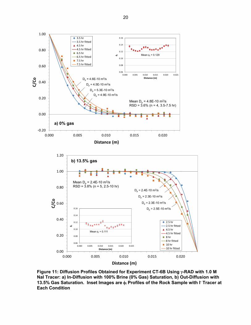
Figure 10: Diffusion Profiles Obtained for Experiment CT-6A Using γ-RAD with 1.0 M NaI Tracer: a) In-Diffusion with 100% Brine (0% Gas) Saturation, b) Out-Diffusion with 15.2% Gas Saturation, and c) In-Diffusion following b). Inset Images are φI Profiles of the Rock Sample with I- Tracer at Each Condition .................................................................................. 19 Figure 11: Diffusion Profiles Obtained for Experiment CT-6B Using γ-RAD with 1.0 M NaI Tracer: a) In-Diffusion with 100% Brine (0% Gas) Saturation, b) Out-Diffusion with 13.5% Gas Saturation. Inset Images are φI Profiles of the Rock Sample with I- Tracer at Each Condition ........................................ 20 Figure 12: Diffusion Profiles Obtained for Sample DGR3-472 Using γ-RAD with 2.0 M NaI Tracer: a) In-Diffusion with 100% Brine (0% Gas) Saturation, b) Out-

Diffusion with 14.6% Gas Saturation. Inset Images are φI Profiles of the Rock Sample with I- Tracer at Each Condition ................................................... 22 Figure 13: Schematic Example of a Modern Harned Cell, Based on the Diagram of

Maksimov et al. (2008) ......................................................................................... 24 Figure 14: Glass Combination pH Electrode ....................................................................... 26 Figure 15: Absorbance Spectra with Changing pH for Phenol Red in L-SPW Tris Buffer Solutions ................................................................................................... 27 Figure 16: Tris Buffer Data: a) Comparison of the pK’a for Tris in Electrolyte Solutions Calculated Using PHREEQC (pitzerUNB Database) with Measured Values for Seawater and the Dead Sea from Millero et al. (1987,

1993). “MacInnes Convention” Means it was Used for Calculating pH in PHREEQC. The Filled Symbols Represent Measured Values and the

Hollow Symbols Represent the Corresponding Calculated Values (Millero et al. 1987); (b) The Modelled pH of a 0.02 mol/kg Tris Buffer in the Same

Solutions Shown in (a) ........................................................................................ 32 Figure 17: Acetate Buffer Data: (a) Comparison Between the Acetate pK’a Calculated

Using PHREEQC (pitzerUNB Database) and Values from Published Literature; (b) The Modelled pH of a 0.002 mol/kg Acetate Buffer in NaCl

Solutions of Varying Ionic Strength. “MacInnes Convention” Means the MacInnes Convention was Used for Calculating pH in PHREEQC ................... 33

Figure 18: Electrode Response to Changing pH for Selected Tris and HCl Buffer Solutions. Modelled pH Values Assume no Equilibrium with Atmospheric CO2(g). Inset: Filled Symbols Represent L-SPW Tris Buffer with No CO2(g)

and Hollow Symbols Represent Modelled pH Assuming Solution Equilibration with CO2(g) (log PCO2 = -3.4) .......................................................... 38 Figure 19: Modelled Versus Measured pH for the Tris Buffer Data Set. Modelled pH

Values Assume no Equilibrium with Atmospheric CO2(g). Data Series with the Identifier “Sureflow” were Measured with the Sureflow Electrode.

Otherwise, the pH was Measured Using the Ross 815600 Electrode ............... 39 Figure 20: The Difference Between Modelled pH and Potentiometrically Measured pH with Changing Ionic Strength and Solution Composition. Modelled Values Do Not Include Equilibration With Atmospheric CO2(g). Vertical Error Bars Represent the Standard Error in Potentiometric pH Measurements, ±0.03 pH Units. Horizontal Error Bars Represent the Standard Deviation in Ionic Strength Across a Buffer Series; Where Not

Visible, the Variation is Smaller than the Symbol .............................................. 40 Figure 21: Measured pH of a L-SPW Tris Buffer Series Over Time. The Data Have

ix

Been Normalized to 25 °C. Error Bars Represent the Standard Error in Potentiometric pH Measurements, ±0.03 pH Units ............................................ 41

Figure 22: Plot of the Phenol Red Absorbance Ratio Versus pH in L-SPW. Filled Symbols Represent Modelled pH Assuming no Equilibrium with Atmospheric CO2(g); Hollow Symbols Represent Modelled pH with Solutions at Equilibrium with Atmospheric CO2(g) (log PCO2 = -3.4) ................ 43 Figure 23: Variation in Phenol Red pK'a with Ionic Strength and Solution Composition. Vertical Error Bars Represent 1σ. Horizontal Error Bars

Represent the Standard Deviation in Ionic Strength Across a Tris Buffer Series; Where Not Visible, the Variation is Smaller than the Symbol .............. 44

x

LIST OF ABBREVIATIONS CT Carbon Tan sandstone Dp Pore diffusion coefficient: Dp=(δ/τ)·D0, where δ is constrictivity, τ is tortuosity,

and D0 is the free water diffusion coefficient De Effective diffusion coefficient: De=ϕDp. DGR Deep geological repository ER Edge Response IUPAC International Union of Pure and Applied Chemistry L-SPW DGR limestone synthetic porewater MIN3P Multicomponent reactive transport code NIST Nation Institute of Standards and Technology NWMO Nuclear Waste Management Organization ODR Optical Density Ratio PHREEQC A computer program for speciation, batch-reaction, one-dimensional transport,

and inverse geochemical calculations pKa Thermodynamic disassociation constant pK’a Conditional disassociation constant RAD Radiography γ-RAD Gamma-radiography RSD Relative Standard Deviation SNR Signal-to-noise ratio SP Spatial Resolution S-SPW DGR shale synthetic porewater TD Through-diffusion Tris Tris-[hydroxymethyl]aminomethane TrisHCl Tris-[hydroxymethyl]aminomethane hydrochloride UNB University of New Brunswick URL Underground research laboratory φI Iodide-accessible porosity φw Water-loss porosity ∆μ Change in attenuation coefficient µbrine Attenuation coefficient of brine–saturated rock µPS Attenuation coefficient for the partially brine-saturated sample µPS-tracer Attenuation coefficient for the partially tracer-saturated sample µtracer Attenuation coefficient of the tracer–saturated rock

1

1. INTRODUCTION This technical report documents activities and outcomes of research performed at the University of New Brunswick between March, 2012 and March, 2014 for the Nuclear Waste Management Organization. The research is intended to continue the development of new methodologies for laboratory measurements of diffusion properties in low permeability rocks and to gain a better understanding of the mechanisms controlling solute transport in diffusion-dominated sedimentary and crystalline rock systems. Such systems are under consideration in Canada as potential host and barrier rocks for a deep geological repository for the long-term management of radioactive waste. The research is grouped into four projects that are presented separately in this report. The first involved improvement of the radiography method of tracer measurement in the estimation of diffusion properties in low permeability rocks by using a monochromatic γ-ray source (γ-RAD) instead of X-rays. One of the main advantages of the γ-RAD technique is to eliminate the beam hardening that occurs with a polychromatic X-ray source. A second advantage of the γ-RAD technique is that it allows for measurements on larger samples and provides greater flexibility in the experimental design. The second project involved development of methods for simultaneous measurement of diffusive tracer profiles in low permeability rocks using both γ-RAD and through-diffusion (TD) methods. This was tested for the first time using a granite sample. In the third project, a method was developed to create partial gas saturation conditions in porous sedimentary rock followed by the measurement of effective diffusion coefficient (De) values. The effect of partial gas saturation on diffusion coefficients was assessed by comparing the De values measured at full brine saturation with those measured at different degrees of partial gas saturation. The fourth project involved development of improved methods for pH measurement in high salinity natural porewaters. Accurate and precise measurement of pH at high ionic strength is important for a range of research activities that seek to quantify water-rock reaction processes (e.g. ion exchange, speciation, surface complexation, and mineral precipitation and dissolution), most of which are sensitive to pH.

2. γ-RADIOGRAPHY METHOD A γ-RAD technique was first developed by Subudhi (2009) and Subudhi et al. (2010) for measurement of porosity and diffusion coefficients of porous media. The method is similar in principle to the X-ray RAD technique (Al et al. 2010; Cavé et al. 2009, Cavé et al. 2010) except that it uses monochromatic gamma radiation from an Am-241 source. This has some advantages over the use of X-rays in that it minimizes or eliminates artefacts from beam hardening and X-ray-beam geometry and there are no restrictions on the sample size. New sample cells were designed and constructed as shown in Figure 1. The cell shown in Figure 1a was used for simultaneous diffusion measurements with γ-RAD and TD methods, and the cell in Figure 1b was used for quantifying the degree of partial gas saturation and for measuring De on rock samples with variable brine-gas saturation states.

The circumference of the cylindrical sample (nominal 20 mm diameter, 13-25 mm height) was wrapped with a thin Teflon® tape (0.02 mm thickness, Green Belting Industries). The seam was sealed with a thin bead of silicone. The sample was pressed into the Delrin® sleeve

2

(Figure 1) and then saturated with a background brine solution (Appendix A). After sample saturation, the diffusion cell was assembled by installing Delrin® caps at each end (Figure 1).

a)

X

Connected to 1/8” OD tubing then to pump


Delrin cap

O-ring

Delrin sleeve

Fluoropolymer tape (0.02 mm thick)

Rock sample (20 mm dia, 25 mm h max)

Internal standard (20 mm thick Mycalex ceramic)

Reservoir

PTFE connector (1/8” OD tubing)

®

®

Gamma ray scan upwards

b)

X



Delrin cap

Reservoir

Delrin sleeve

Fluoropolymer tape (0.02 mm thick)

Rock sample (20 mm dia, 25 mm h max)

Internal standard (20 mm thick Mycalex ceramic)

Position pinO-ring (3/32 thick, 1 3/16 ID viton dash#123)

PTFE connector (1/16” OD tubing, 1/16 NPT thread)

®

®

Gamma ray scan upwards

Figure 1: Sample Cell Designs for γ-RAD Experiments: (a) Sample Cell for Simultaneous Measurements Using γ-RAD and TD Techniques, (b) Sample Cell Used for Partial Saturation Experiments

3

Mycalex® ceramic was used for an internal standard because it has similar density and γ attenuation to the experimental rock materials (Loomer et al. 2013a). The internal standard was fixed to the side of the cell. The radiation path along the rock sample is shown in Figure 1. The length of the radiation path is 20 mm for both the rock samples and for the ceramic standard. The diffusion cell was mounted on a stage controlled by an automated stepping motor (BiSlide® Velmex Inc.; Figure 2). Positioning pins were constructed on the stage so that the cell can be removed and replaced in the same position during the experiments.

Figure 2: Photograph of the γ-RAD System: The Am-241 γ-Ray Source is Visible at Left (Yellow), the Sample Cell is Mounted on a Computer-Controlled Stage in the Middle, and the Tl-NaI Detector is Encased in a Painted (Beige) Pb Brick at Right. Note that the Source Collimator was Removed for the Photo but the Detector Collimator is in Place

The system employs an Am-241 sealed source (11.1 GBq), a Tl-NaI detector (Canberra model 802) powered by a Tennelec model TC950 detector bias supply, and a Tennelec model TC246 amplifier and single channel analyzer. The source and detector collimation, and the source-detector alignment are described by Subudhi et al. (2010). The operating parameters are presented in Table 1. The spatial resolution of the measurements (1.4 to 1.5 mm diameter) was determined using an Edge Response (ER) technique (Smith 2003; Hussein 2011). The ER measures how an instrument responds to a sharp discontinuity and involves collecting a line profile across the boundary of two sharply contrasting materials or media (such as the edge of a solid material and air). The spatial resolution is taken to be the distance required for the profile to rise from 10% to 90% of the difference in the values of the two contrasting materials or media. In this case the spatial resolution was determined by scanning (0.25 mm step size) across the sharp edge of a 3-mm-thick steel bar positioned on the sample stage (Figure 3).

4

Table 1: Am-241 γ-RAD Operating Parameters

Collimator diameter 3.0 mm

Sample thickness 20 mm

Source-detector distance 10 mm

Detector-sample distance 4 mm

Source collimator length 10.0 mm

Detector collimator length 95 mm

Detector Output voltage 1700 V

Coarse gain 50

Fine gain 8

Overall gain 50 x 0.8 = 40

Stage increments (X,Z) 200 per 1.0 mm

Spatial resolution (diameter) 1.4 - 1.5 mm

Measurement step size (mm) 0.5 - 1.0

Scan time/point (s) 35 – 60

0

5000

10000

15000

20000

25000

30000

35000

0 2 4 6 8 10 12

Cou

nts

per s

econ

d (C

PS)

Distance (mm)

SR=1.5 mm

Figure 3: Estimation of Spatial Resolution (SR) for γ-RAD Technique

5

The radiography method for measuring diffusion coefficients uses a blank subtraction approach (Al et al. 2010; Cavé et al. 2009; Cavé et al. 2010) to remove the constant background attenuation effects of the porous matrix. Time-series radiographs (samples with tracer at t > 0) are subtracted from a reference radiograph (sample without tracer at t = 0) to determine the change in attenuation due to tracer mass in the pores, which we define as the parameter Δµ:

∆µx = ln(Iref)x – ln(It)x = (µp t=0 – µp t>0)x φx (1) where: t is time, (Iref)x is the transmitted γ-ray intensity at distance x on the t = 0 (reference) profile, (It)x is the transmitted γ-ray intensity at the same distance on one of the time-series profiles (t > 0), µp t=0 and µp t>0 are the attenuation coefficients of the pore fluids in the reference and time-series radiographs, respectively. The parameter ∆µ is a function of the mass of tracer along the γ-ray path and is used to determine quantitative measurements of tracer concentration (Al et al. 2010; Cavé et al. 2009; Cavé et al. 2010). There is significant ambiguity in the literature in terms of diffusion-related terms, so the following definitions are provided for clarity:

(2) where: D0 is the free-water diffusion coefficient and τf is the tortuosity factor,

(3) where: φ is porosity.

2.1 CALIBRATION Calibration curves for ∆µ as a function of I- concentration were generated by the method reported by Cavé et al. (2009) using the sample cell (Figure 1) filled with a series of brine/tracer standard solutions. The ∆µ values were normalized to the diameter of the rock samples, which is slightly smaller than the inner diameter of the Delrin® sleeve. Results of the calibration in a 1.0 M NaNO3 matrix and in a much more saline S-SPW matrix (shale synthetic porewater, see Table 4) are presented in Figure 4. This relationship is linear over a range of ∆µ up to approximately 2 and the slope is almost independent of the background matrix. In contrast, calibration curves obtained with X-ray radiation are affected by beam hardening which results in non-linear relationships and matrix dependency.

6

y = 1.7858xR² = 0.9991

0.0

0.5

1.0

1.5

2.0

0.0 0.2 0.4 0.6 0.8 1.0 1.2

∆ µ

I- Concentration (mol/L)

NaNO3 matrixS-SPW matrix

Figure 4: Calibration between ∆µ and I- Concentration Using the γ-RAD Technique

2.2 SUMMARY The use of monochromatic Am-241 γ radiation eliminates beam hardening, providing a precise calibration function. Results of calibration indicate a linear function over a large range in ∆µ that is not sensitive to the background matrix. The method is appropriate for measurements of tracer concentration in cases where spatial resolution on the order of 1 mm or greater is satisfactory.

7

3. DIFFUSION MEASUREMENTS WITH GRANITE

3.1 METHODS A test was conducted to determine the potential for using the γ-RAD method for measuring diffusion coefficients of crystalline rocks such as granite. The testing was conducted on archived granite sample from the Atomic Energy of Canada Limited Whiteshell Research Area, specifically a segment of borehole 209-069-PH3 (sample OPG-10 from Cavé and Al 2006). A subsample, 20 mm in diameter, was prepared by diamond coring and then the sample was mounted in the modified diffusion cell (Figure 1a) which allows for simultaneous measurements by TD and by γ-RAD methods. The sample was saturated with NaNO3 (4 mol/L) solution by immersion (mounted in the Delrin® sleeve) under vacuum for 3 days (Appendix A). The cell was then assembled and 4 mol/L NaNO3 solution was circulated through both ends for 8 additional days. The concentration of the I- tracer and the scanning parameters (Table 2) were selected to provide sufficient contrast for the γ-RAD method. The TD measurements were conducted according to the methods previously described by Cavé et al. (2010) and Xiang et al. (2013).

Table 2: γ-RAD Experimental Conditions

Sample Carbon Tan Queenston shale Granite Scan time/point (s) 35 35 60 Measurement Step Size (mm) 1.0 0.75 0.5 Synthetic Pore Fluid 1.0 M NaNO3 S-SPWa 4.0 M NaNO3 Tracer 1.0 M NaI 2.0 M I- in S-SPWb 4.0 M NaI a Shale synthetic porewater, Table 4; b Equal moles of NaCl were substituted by NaI in S-SPW.

3.2 RESULTS The γ-RAD measurements (Figure 5) display a large degree of scatter due to the low porosity and the resulting small mass of tracer contained in the sample. Efforts to enhance the signal to noise ratio (SNR) included the use of long counting times and high tracer concentration (Table 2). Despite the scatter in the data it is possible to identify tracer profiles that advance with time, and an average pore diffusion coefficient (Dp) value of 7.2×10-11 m2/s is obtained. For the purpose of comparison, this Dp value can be multiplied by φI (0.0043) (iodide accessible porosity) to obtain a De value of 3.1×10-13 m2/s which is consistent with measured diffusion coefficients for crystalline rocks from Manitoba Canada, Sweden and Finland (Table 3). A through-diffusion (TD) experiment was conducted simultaneously, and the early-time trends in the tracer flux and cumulative mass data (<13 days; Figure 6) evolved according to expectations. However, beyond 13 days the tracer flux decreases in a way that is inconsistent with steady-state diffusion. This behaviour is thought to result from gradual occlusion of diffusion pathways due to mineral-water reactions. Although the early time data (<13 days) indicate a De value of 3.0×10-13 m2/s which is very close to the value obtained by γ-RAD,

8

confidence in this result is low because of the unexpected decline in the tracer flux after 13 days.

-0.20

0.00

0.20

0.40

0.60

0.80

1.00

0.000 0.002 0.004 0.006 0.008 0.010 0.012 0.014

Distance (m)

3.5 hr3.5 hr fitted26 hr26 hr fitted37 hr37 hr fitted

0.000

0.002

0.004

0.006

0.008

0.010

0.000 0.005 0.010 0.015

Distance (m)

C/C 0

φI

D = 1.0 x 10 m /sp-10 2

D = 5.5 x 10 m /sp-11 2

D = 6.0 x 10 m /sp-11 2

Average D = 7.2 x 10Average D = 3.1 x 10 m /s

p-11

e-13 2

m /s2

Average = 0.0043 (0.43%)

Figure 5: Diffusion Profiles in Granite Obtained by γ-RAD with 4.0 M NaI Tracer. Inset: φI Profile of the Rock Sample

0.01.02.03.04.05.06.07.08.09.0

10.0

0 5 10 15 20 25 30

Flux

of I

-(m

mol

m-2

d-1

)

Time (d)

a)

0

0.01

0.02

0.03

0.04

0.05

0.06

0 5 10 15 20 25 30

Cum

ulat

ive

I-(m

mol

)

Time (d)

b)

De = 3.0x10-13 m2/sφI = 0.27 %

Figure 6: Results of Through-diffusion Experiment with Granite: (a) Flux of I- Tracer and (b) Cumulative I- Quantity as a Function of Time. This Experiment was Conducted Simultaneously with the γ-RAD Experiment (Figure 5)

9

Table 3: Literature Values of Diffusion Properties Obtained by Through-diffusion Experiments for Crystalline Rocks

Location Rock type Porosity De (m2/s) Exp. condition Ref.

Canada, URL Manitoba

Granite, granodiorite

0.22-0.28% (H2O immersion), 0.46 - 0.94% (I-; TD)

2.1x10-12 to 1.9x10-13 in situ, I- a

2.2x10-12 to 2.7x10-12 Lab, I-

Sweden central, east coast

Granite, granodiorite

7.0x10-12 to 1.3x10-13 lab, I- b

1.3x10-13 to 1.8x10-13 lab, HTO

Sweden, Aspo lab Diorite and granite 0.36 - 0.84% 1x10-13 to 9x10-13 lab, I-, HTO c

Finland Tonalite and mica gneiss

0.1 - 3% (tonalite) 0.2% (mica gneiss)

3.0x10-12 to 9x10-13 1.0x10-12 to 6x10-13

lab, TD, HTO lab, TD, Cl- d

a Vilks et al. 2003; b Skagius and Neretnieks 1986; c Xu et al. 2001 and Johansson et al. 1998; d Siitari-Kauppi et al 1997.

10

3.3 SUMMARY The γ-RAD method has been tested for potential use in measurement of De values for crystalline rock samples. The result is consistent with the range of values obtained for crystalline rocks elsewhere. The result is also in good agreement with the De value obtained with simultaneous measurement by TD on the same sample (3.0×10-13 m2·s-1 and 3.1×10-13 m2·s-1, respectively). However, there is low confidence in the TD measurement. This is the first and only test of the radiography method on low-porosity crystalline rocks and, although further improvements are possible, the results suggest that it is a viable approach.

4. EFFECT OF PARTIAL GAS SATURATION ON DIFFUSION Results of site characterization studies at the Bruce nuclear site suggest that at some depths in the Ordovician shales and limestones the porewater saturation may be less than 100% and the pore volume may be occupied by a mixture of porewater and gas (Intera, 2011). Partial gas saturation may result from the formation of methane by thermogenic or biogenic mechanisms. Pore-scale changes in the volume ratio of gas and porewater are expected to affect De for both aqueous solutes and gases (Savoye et al. 2010). In this study, our objectives are: • to develop a method to create partial saturation in rock samples for use in testing of the γ-

RAD technique; • to determine the degree of the partial saturation using the γ-RAD technique; and, • to investigate the effect of partial saturation on De in low permeability rocks. Sedimentary rocks may contain highly saline porewater, and experimental methods for generating partial saturation must not cause dewatering which could lead to the precipitation of salts, occlusion of porosity and artefacts in De measurements.

4.1 BACKGROUND: CREATING PARTIAL GAS SATURATION The approach to creating partial-gas-saturated conditions in rock samples uses N2 gas and takes advantage of the variability of N2 solubility versus pressure. The solubility of a gas in aqueous solution at a given temperature is proportional to its partial pressure. This is known as Henry’s law:

Si = KH • Pi (4)

where Si is the solubility of gas i (mol/L) in an aqueous solution; KH is the Henry’s law constant (mol•L-1•atm-1 or M/atm) for gas i in the solution; Pi is the partial pressure of gas i (atm). The constant KH is dependent on the gas, the temperature and the solution composition. The partial saturation experiments described herein are conducted at 25 ºC using N2 gas and synthetic porewater solution (1.0 mol/L NaNO3 solution for the Carbon Tan sandstone and shale synthetic porewater, S-SPW, for the Queenston Formation shale, Table 2). The composition of S-SPW (Table 4) was adapted from previous work on shale samples (Al et al. 2010, 2012; Cavé et al. 2010; Loomer et al. 2013b; Xiang et al. 2013). The solubility of N2 at 25 ºC as a

11

function of partial pressure (PN2; Figure 7) was calculated with the empirical model reported by Mao and Duan (2006) for N2 solubility in NaCl solutions up to 5.3 mol/L. Model calculations were conducted using 1.0 mol/L NaCl solution as a proxy for the 1.0 mol/L NaNO3 Carbon Tan sandstone porewater. Model calculations for the Queenston shale porewater were conducted at the 5.3 mol/L (NaCl solution) limit of the model although the S-SPW is actually a Na-Ca-Cl solution with 5.8 mol/L Cl-. As a result, the model calculations do not fully represent the experimental system, and particularly for the S-SPW case, it is expected that the N2 solubility in S-SPW will be overestimated by the model.

Table 4: Composition of Synthetic Porewater (SPW) Solutions Used at UNB

S-SPW L-SPW

(mol/kg) (mol/kg)

Na+ 2.71 2.18 K+ 0.56 0.49 Ca2+ 1.36 0.53 Mg2+ 0.28 0.22 Cl- 6.55 4.16 SO4

2- 0.001 0.005 Ionic Strength 8.2 4.9

y = 0.000602 x

y = 0.000163 x

y = 0.000473x

0.00

0.01

0.02

0.03

0.04

0.05

0.06

0.07

0.08

0.09

0.10

0 20 40 60 80 100 120 140

N2

gas

solu

bilit

y (m

ol/L

)

PN2 (atm)

25 C water

25 C 1.0 mol/L NaCl

25 C 5.3 mol/L NaCl

Figure 7: Henry’s Law Plots for N2 Gas at 25 ˚C in Water, 1.0 mol/L NaCl and 5.3 mol/L NaCl Solutions Calculated Using the Empirical Model Reported by Mao and Duan (2006). The Slopes Correspond to the Henry’s Law Constants (KH)

12

Data in Figure 7 indicate that N2 solubility in 1.0-5.3 mol/L NaCl brines obeys Henry’s law up to a partial pressure of 60-70 atm (filled symbols), after which (open symbols) there is a slight departure from linearity. The KH values determined are 0.000473 M/atm for 1.0 mol/L NaCl brine and 0.000163 M/atm for 5.3 mol/L NaCl. When a brine system undergoes a change in N2 partial pressure from high (P1) to low (P2), the solubility of N2 decreases correspondingly from S1 to S2. As a result, gas bubbles will form in the solution. For the brine solution occupying the pore spaces in a rock sample, gas bubbles should form in the pore spaces, causing partial brine saturation. Assuming equilibrium is established at P2, the moles of N2 bubbles, n, can be calculated according to:

nbubble = KHVp(P1-P2) (5)

where Vp is the volume of the rock pores (L) initially occupied by brine. The volume of the gas bubbles (Vbubble) formed at P2 can be calculated using the ideal gas law:

Vbubble = nbubbleRT/P2 = KHVp(P1-P2)RT/P2 (6)

The bubble volume calculated by this method was compared to the bubble volume calculated using Van der Waal’s equation for non-ideal gases. A maximum difference between two methods of 0.07% was noted under the experimental conditions. Assuming bubbles are formed and remain in the rock pores (the volume change is accounted for by expulsion of brine from the pores), the relative pore volume occupied by gas (% gas saturation) will be:

% gas saturation = [KH(P1-P2)RT/P2] x 100% (7)

Experiments were designed so that P2 was equal to 1 atm of N2 (moisturized). Values for the % gas saturation as a function of P1 (Table 5) were calculated using Equation 7. The calculations included P1 values beyond the linear region in Figure 7 (>60-70 atm) assuming Henry’s law still applies.

13

Table 5: Relationship between % Gas Saturation and Initial N2 Pressure (P1)

1.0 M NaCl 5.3 M NaCl % gas sat. P1 P1 P1 P1 (atm) (kPa) (atm) (kPa)

2 2.6 268 5.8 591 5 5.2 522 13.1 1329 10 9.3 947 25.3 2560 20 17.7 1795 49.6 5022 25 21.9 2219 61.7 6253 30 26.1 2643 73.9 7484 35 30.3 3068 86.0 8715 40 34.5 3492 98.2 9946 45 38.6 3916 110.3 11177 50 42.8 4340 122.5 12408 55 47.0 4765 134.6 13639 60 51.2 5189 146.8 14870 70 59.6 6037 171.1 17332 80 68.0 6886 195.4 19794 90 76.3 7734 219.7 22256

aData were calculated using Equation 7 under the following conditions: T = 25 °C, P2 = 1.0 atm N2, 1.0 mol/L or 5.3 mol/L NaCl brine with a KH constant of 0.000473 mol L-1 atm-1 or 0.000163 mol L-1 atm-1 (Figure 7), respectively.

Estimates of % gas saturation from Equation 7 represent the maximum attainable values. The actual degree of partial saturation achieved by experiment is expected to be lower because some N2 may be lost from the system by diffusion while the system re-equilibrates from P1 to P2. The actual degree of partial saturation is determined by the γ-RAD method.

4.2 EXPERIMENTAL PROCEDURES Samples used in the investigation of partial gas saturation include one sample of Carbon Tan sandstone that was used in two experiments, one after the other (CT-6A and CT-6B) and a sample of Queenston Formation shale (DGR3-472). The experimental procedures are as follows:

• The samples were saturated according to the methods described in Appendix A using a synthetic pore fluid (1.0 mol/L NaNO3 for the Carbon Tan sandstone and S-SPW for the Queenston Formation shale), installed in a Delrin® diffusion cell (Figure 1b).

• The initial reference scan was conducted prior to the introduction of tracer, which provides a measure of the γ attenuation properties of the brine–saturated rock (µbrine).

• The samples were submerged in the tracer solution (Table 2) and allowed to saturate with I- tracer after which γ-RAD scans were conducted to measure the γ attenuation properties of the tracer–saturated rock (µtracer).

14

• The solution containing the samples was then placed in a chamber pressurized with N2 gas (P1, Table 6). The system was allowed to equilibrate for up to 27 days, after which time the N2 pressure in the chamber was decreased to one atmosphere (P2), the sample was removed from the tracer solution and the diffusion cell was quickly re-assembled (<15 minutes).

• Moisturized N2 gas (~1 atm) was pumped through both reservoirs (~15 mL/min) and radiography scans were recorded to monitor the displacement of tracer solution from the sample due to formation of N2 gas bubbles. It took between five and ten hours for this process to stabilize in the Carbon Tan sandstone sample, and 48 hours in the Queenston shale sample.

• Fresh tracer solution (1.0 M I- for Carbon Tan sandstone and 2.0 M I- for Queenston Formation shale) was then allowed to circulate through both reservoirs for up to eleven days to ensure that the brine/gas saturation states had stabilized. Three scans were conducted before starting the diffusion experiment and the average of these scans (µPS-

tracer) provides a reference for the diffusion experiment to measure De for the partially saturated sample. This measurement was conducted as an “out-diffusion” experiment whereby synthetic pore fluid was introduced to one reservoir and tracer was allowed to diffuse out of the sample.

• After the out-diffusion measurement, the remaining I- tracer was removed by circulating synthetic pore fluid through both reservoirs while recording radiography scans periodically to confirm complete removal.

• After tracer removal, three final scans were recorded (µPS-brine) to complete the multi-step experiment.

A quantitative measure of the degree of partial gas saturation is obtained as:

(8)

Where subscripts ps and S indicate partially-saturated and saturated conditions respectively. For the purpose of comparison, an in-diffusion experiment was conducted following the out-diffusion experiment (CT-6A and CT-6B respectively).

Table 6: Experimental Conditions Used for Partial Gas Saturation Experiments

Experiment ID CT-6A CT-6B DGR3-472

P1 (kPa) 4400 6600 7000 T (oC) 23 ± 2 22.5 ± 0.5 23 ± 1 Predicted % gas saturation (from Table 5) 50 80 28

15

4.3 RESULTS AND DISCUSSION

4.3.1 Partial Gas Saturation

4.3.1.1 Carbon Tan Sandstone One-dimensional profiles of ∆µ that reflect the distribution of I- tracer mass in the rock samples are compared before and after establishment of partial gas saturation (Figure 8a). The concentration of I- in the porewater remains constant so the systematic shift of the profiles to lower ∆µ values is consistent with a decrease in porewater volume. Profiles of ∆µ have been converted to that of φI (Figure 8b) using the calibration function of the γ-RAD method (Section 2.1). These results demonstrate that there is a near-uniform displacement of pore fluid due to formation of a discrete gas phase. Measurements indicate that the average partial gas saturation is 15.2% (84.8% brine) for experiment CT-6A and 13.5% (86.5% brine) for experiment CT-6B calculated by equation 8 (Table 7). These percentages are much lower than the predictions (50% and 80% respectively; Table 6). The discrepancy between predicted and measured values may be explained by non-ideal effects that are not accounted for in the ideal-gas law or the Van der Waal equation. Perhaps most importantly, the tendency to form a discrete gas phase in the pore space will be limited by the permeability, which controls the rate of pore fluid displacement by the expanding gas bubbles.

0.12

0.14

0.16

0.18

0.20

0.22

0.24

0.26

0.28

0.000 0.005 0.010 0.015 0.020

∆µ

Distance (m)

CT-6A 100% Brine CT-6B 100% BrineCT-6A 15.2% Gas CT-6B 13.5% Gas

a)

0.06

0.08

0.10

0.12

0.14

0.16

0.000 0.005 0.010 0.015 0.020

φ I

Distance (m)

CT-6A 100% Brine CT-6B 100% BrineCT-6A 15.2% Gas CT-6B 13.5% Gas

b)

Figure 8: One Dimensional Profiles of a) ∆µ and b) φI of 1 M I- Tracer in Carbon Tan Sandstone (Experiments CT-6A and CT-6B) before and after Establishment of Partial Gas Saturation. Error Bars Represent the Standard Deviation Measured on Replicate Scans over a Period of up to 7 Days

16

Table 7: Properties of Variably Saturated Carbon Tan Sandstone

Experiment CT-6A CT-6A-PSa CT-6B CT-6B-PSa

Δμ (1 M I-) 0.231 0.196 0.230 0.199

φI (brine)b 0.129 0.110 0.129 0.111

% Brine Saturation 100 84.8 100 86.5

% Gas Saturation 0 15.2 0 13.5

Dp (m2/s) 4.1E-10 3.9E-10c 4.8E-10 2.4E-10

De (m2/s) 5.3E-11 4.2E-11c 6.2E-11 2.7E-11 a PS indicates samples with partial gas saturation; b brine-filled porosity determined by γ-RAD; c average of values determined by in- and out-diffusion experiments.

4.3.1.2 Queenston Formation Shale Profiles representing the distribution of I- tracer in the shale sample before and after establishment of partial gas saturation (Figure 9) indicate a general shift to lower I- mass, in a similar manner to the sandstone samples. Unfortunately, data in Figure 9 also indicate that sample breakage occurred at a distance of 0.015 m. The sample separated along the bedding plane, presumably due to the build-up of gas pressure that could not be relieved by pore fluid displacement because of the low permeability of the rock. This problem can be avoided with some minor modifications to the diffusion cell design. Results of measurements reported in Table 8 for this partially-gas saturated sample were obtained from the data collected in the 0-0.015 m portion of the sample. Measurement of the degree of partial gas saturation indicates 14.6% (85.4% brine). Once again, this percentage is lower than predicted (28%, Table 6).

0.10

0.15

0.20

0.25

0.30

0.35

0.40

0.000 0.005 0.010 0.015 0.020

∆µ

Distance (m)

0% Gas14.6% Gas

a)

0.03

0.05

0.07

0.09

0.11

0.000 0.005 0.010 0.015 0.020

φ I

Distance (m)

0% Gas14.6% Gas

b)

Figure 9: One Dimensional Profiles of a) ∆µ and b) φI of 2 M I- Tracer in Queenston Shale Sample (DGR3-472) before and after Establishment of Partial Gas Saturation. Error Bars Represent the Standard Deviation Measured on Replicate Scans over a Period of 4 Days

17

Table 8: Properties of Variably Saturated Queenston Formation Shale

Sample DGR3-472 DGR3-472-PSa

Δμ (2 M I-) 0.261 0.223

φI (brine)b 0.073 0.063

% Brine Saturation 100 85.4

% Gas Saturation 0 14.6

Dp (m2/s) 4.4E-11 2.3E-11

De (m2/s) 3.2E-12 1.5E-12

a PS indicates samples with partial gas saturation; b brine-filled porosity determined by γ-RAD.

4.3.2 Effect of Partial Gas Saturation on Diffusion Coefficients

4.3.2.1 Carbon Tan Sandstone Measurements for experiment CT-6A indicate that Dp for I- tracer in a 100% brine-saturated sample is 4.1 x 10-10 m2/s (Figure 10a), and at 15.2% gas saturation the Dp value decreases to 3.9 x 10-10 m2/s (average of results from out-diffusion and in-diffusion experiments; Figure 10b,c). These results suggest that the effect of approximately 15% gas is small - only a 5% decrease in Dp. In contrast, data for experiment CT-6B indicate a 50% decrease in Dp for the same sample at a slightly lower gas saturation (13.5%; Figure 11a, b). The large difference between two measurements using the same rock sample is surprising and suggests an unidentified source of error or a difference in the gas distribution at the pore scale that is not apparent in the φI profiles (Figures 8, 10 and 11). For example, a predominance of gas bubbles in the pore throats for experiment CT-6B could contribute to a relative decrease in the tortuosity factor (τf) and explain the lower Dp value observed for the partially saturated sandstone. The De values for aqueous solutes are further affected by the decrease in brine-filled porosity (Table 7) such that partial gas saturation resulted in decreases in De of 21% and 56% for experiments CT-6A and CT-6B respectively. The addition of a gas phase to the pores is also expected to cause an increase in diffusion coefficients for gases (Reardon and Moddle 1985), but this effect has not been quantified in these experiments.

18

0.06

0.08

0.10

0.12

0.14

0.16

0.000 0.005 0.010 0.015 0.020 0.025

I

Distance (m)

‐0.20

0.00

0.20

0.40

0.60

0.80

1.00

0.000 0.005 0.010 0.015 0.020

C/Co

Distance (m)

3.5 hr3.5 hr fitted5 hr5 hr fitted7 hr7 hr fitted8.5 hr8.5 hr fitted

Mean Dp = 4.1E-10 m2/sRSD = 8.7% (n = 4, 3.5-8.5 hr)

a) 0% gas

Dp = 3.8E-10 m2/s

Dp = 3.8E-10 m2/s

Dp = 4.5E-10 m2/s

Dp = 4.3E-10 m2/s

Mean I = 0.129

0.06

0.08

0.10

0.12

0.14

0.16

0.000 0.005 0.010 0.015 0.020 0.025

I

Distance (m)

0.00

0.20

0.40

0.60

0.80

1.00

1.20

0.000 0.005 0.010 0.015 0.020

C/Co

Distance (m)

1.5 hr 1.5 hr fitted3 hr 3 hr fitted4.5 hr 4.5 hr fitted5.5 hr 5.5 fitted7 hr 7 hr fitted10.5 hr 10.5 hr fitted

Mean I = 0.110

b) 15.2% gas


Dp = 3.6E-10 m2/s

Dp = 2.9E-10 m2/s

Dp = 3.7E-10 m2/s

Dp =3.3E-10 m2/s

Dp =4.3E-10 m2/s

Dp = 4.0E-10 m2/s

19

-0.20

0.00

0.20

0.40

0.60

0.80

1.00

0.000 0.005 0.010 0.015 0.020

C/Co

Distance (m)

2 hr2 hr fitted3 hr3 hr fitted4 hr4 hr fitted6 hr6 hr fitted

c) 15.2% gas

Mean Dp = 3.9E-10 m2/sRSD = 4.7% (n = 4, 2-6 hr)Dp = 4.0E-10 m2/s

Dp = 3.8E-10 m2/s

Dp = 4.1E-10 m2/s

Dp = 3.7E-10 m2/s

Figure 10: Diffusion Profiles Obtained for Experiment CT-6A Using γ-RAD with 1.0 M NaI Tracer: a) In-Diffusion with 100% Brine (0% Gas) Saturation, b) Out-Diffusion with 15.2% Gas Saturation, and c) In-Diffusion following b). Inset Images are φI Profiles of the Rock Sample with I- Tracer at Each Condition

20

0.06

0.08

0.10

0.12

0.14

0.16

0.000 0.005 0.010 0.015 0.020 0.025

I

Distance (m)

‐0.20

0.00

0.20

0.40

0.60

0.80

1.00

0.000 0.005 0.010 0.015 0.020

C/Co

Distance (m)

3.5 hr3.5 hr fitted4.5 hr4.5 hr fitted6.5 hr6.5 hr fitted7.5 hr7.5 hr fitted


Dp = 4.5E-10 m2/s

Dp = 4.6E-10 m2/s

Dp = 5.3E-10 m2/s

Dp = 4.9E-10 m2/s

a) 0% gas

Mean I = 0.129

0.06

0.08

0.10

0.12

0.14

0.16

0.000 0.005 0.010 0.015 0.020 0.025

I

Distance (m)0.00

0.20

0.40

0.60

0.80

1.00

1.20

0.000 0.005 0.010 0.015 0.020

C/Co

Distance (m)

2.5 hr2.5 hr fitted4.5 hr4.5 hr fitted8 hr8 hr fitted10 hr10 hr fitted

Mean Dp = 2.4E-10 m2/sRSD = 3.8% (n = 5, 2.5-10 hr)

b) 13.5% gas

Dp = 2.4E-10 m2/s

Dp = 2.3E-10 m2/s

Dp = 2.3E-10 m2/s

Dp = 2.5E-10 m2/s

Mean I = 0.111

Figure 11: Diffusion Profiles Obtained for Experiment CT-6B Using -RAD with 1.0 M NaI Tracer: a) In-Diffusion with 100% Brine (0% Gas) Saturation, b) Out-Diffusion with 13.5% Gas Saturation. Inset Images are I Profiles of the Rock Sample with I- Tracer at Each Condition

21

4.3.2.2 Queenston Formation Shale Measurements with the Queenston Formation shale (DGR3-472) are preliminary and must be viewed with caution because the problems experienced with sample breakage. The results indicate that Dp for I- tracer at 100% brine-saturation is 4.4 x 10-11 m2/s (Figure 12a) which is consistent with the range of values obtained by previous studies (Al et al. 2010, 2012; Cavé et al. 2010; Xiang et al. 2013). Measurements on the intact portion of the broken sample indicate that Dp decreases to 2.3 x 10-11 m2/s at 14.6% gas saturation (Figure 12b). In terms of De, 14.6% gas saturation causes a decrease of 53%, from 3.2 x 10-12 m2/s to 1.5 x 10-12 m2/s (Table 8). This decrease is lower than that observed by Savoye et al. (2010) who report a 96.5% decrease in De for I- in the Callovo-Oxfordian argillite at 14% gas saturation. Assuming these results can be supported by further work, it is apparent that the degree of partial saturation is one of the more important controls on the magnitude of aqueous diffusion coefficients. For comparison, previous work studying the effect of changes in confining pressure on De noted a maximum decrease in De of 44% for Georgian Bay Formation shale measured at ambient laboratory pressure versus a confining pressure of 15.1 MPa (Loomer et al. 2013a).

4.4 SUMMARY A new method has been developed to generate partial gas and brine saturated conditions in rock samples containing highly concentrated brine without causing changes to the porosity and pore structure from precipitation of salts. The method is based on the relationship between N2 gas solubility and pressure. The porewater system is equilibrated with N2 gas at high pressure and then the pressure is rapidly decreased to atmospheric pressure. This causes a corresponding decrease in gas solubility, resulting in exsolution of N2 to form gas bubbles in the pore spaces. The actual degree of partial gas saturation cannot be predicted accurately by calculations using theoretical P-V-T relationships for gases, but it can be quantified by γ-RAD. Results of De measurements for I- tracer on partially saturated sandstone with gas fractions of 15.2% and 13.5% indicate decreases of 21% and 56% respectively. Preliminary results of measurements on the low-permeability Queenston Formation shale indicate a decrease in De from 3.2 x 10-12 m2/s at 100% brine saturation to 1.5 x 10-12 m2/s at 14.6% gas (85.4% brine) for an overall decrease of 53%.

22

0.02

0.04

0.06

0.08

0.10

0.000 0.005 0.010 0.015 0.020 0.025

I

Distance (m)

‐0.20

0.00

0.20

0.40

0.60

0.80

1.00

0.000 0.005 0.010 0.015 0.020

C/Co

Distance (m)

4.5 hr4.5 hr fitted17 hr17 hr fitted29 hr29 hr fitted45 hr45 hr fitted

Mean Dp = 4.4E-11 m2/s; De = 3.2E-12 m2/sRSD = 4.7% (n = 11, 4.5-45 hr)

Mean I = 0.073

Dp = 4.5E-11 m2/s

Dp = 4.2E-11 m2/s

Dp = 4.5E-11 m2/s

Dp = 4.6E-11 m2/s

a) 0% gas

0.03

0.05

0.07

0.09

0.11

0.000 0.005 0.010 0.015 0.020

I

Distance (m)

0.00

0.20

0.40

0.60

0.80

1.00

1.20

0.000 0.005 0.010 0.015 0.020

C/Co

Distance (m)

9 hr9 hr fitted20.5 hr20.5 hr fitted24.5 hr24.5 hr fitted42 hr42 hr fitted

b) 14.6% gas

Mean I = 0.063

Mean Dp = 2.3E-11 m2/s; De = 1.5E-12 m2/sRSD = 18% (n = 6, 7-42 hr)

Dp = 2.0E-11 m2/s

Dp = 2.2E-11 m2/s

Dp = 2.8E-11 m2/s

Dp = 2.9E-11 m2/s

Figure 12: Diffusion Profiles Obtained for Sample DGR3-472 Using -RAD with 2.0 M NaI Tracer: a) In-Diffusion with 100% Brine (0% Gas) Saturation, b) Out-Diffusion with 14.6% Gas Saturation. Inset Images are I Profiles of the Rock Sample with I- Tracer at Each Condition

23

5. PH MEASUREMENT IN HIGH IONIC STRENGTH BRINE SOLUTIONS Solution pH is a fundamental parameter for understanding the geochemical behaviour of many solutes in groundwater. Reliable pH measurements are important to support studies of speciation, solubility and sorption of radionuclides related to a deep geological repository (DGR) for radioactive nuclear waste. In Canada, Ordovician rocks in the Michigan Basin have been evaluated as possible host rocks for a DGR for low- and intermediate-level waste, and similar rocks are also under consideration as the possible host for a spent nuclear fuel repository. The porewater in these formations is highly saline (up to 28 wt% salinity), with ionic strengths up to 8 mol/kg or higher. The conventional potentiometric method for pH measurement is commonly used for dilute solutions (0.1 m or less), and there is a need for an evaluation of available methods for pH measurements in high salinity brine solutions. Originally, pH was defined simply as the negative logarithm of the hydrogen ion concentration (mH) without consideration of ion interactions in the solution (Equation 9; Jensen 2004). The definition was subsequently modified to the negative logarithm of the H+ activity (aH), but in practice, mH is easier to work with. Many researchers then created application-specific pH scales by adjusting mH to account for certain known interactions between anions and the H+ ion in concentrated solutions (Covington and Ferra 1994; Dickson 1984; Hansson et al. 1973; Millero et al. 1993). This has led to multiple alternative pH scales and some confusion when comparing pH values reported in the published literature. Three common pH scales include the free hydrogen ion scale (pHF), which is simply based on the concentration of free, or uncomplexed, H+ ions (mH; Equation 9); the total hydrogen ion scale (pHT), which accounts for hydrogen ion complexation with sulphate (Equation 10); and the seawater scale (pHSWS), which accounts for H+ interactions with both sulphate and fluoride ions (Equation 11) (Millero et al. 1993).

pHF = −log mH (9)

pHT = −log mH* , where mH* = mH + mHSO4- (10)

pHSWS = −log mH**, where mH** = mH + mHSO4- + mHF- (11)

In 2002, the International Union of Pure and Applied Chemistry (IUPAC; Buck et al. 2002) provided an official definition of pH based on the activity of H+:

pH = −log aH = −log(mHγH/m°) (12)

where γH is the molal activity coefficient of the hydrogen ion, H+, and m° is the standard molality (1 mol/kg). In dilute solutions γH approaches 1 and, therefore mH ≈ aH. However, as solutions become more saline and ion interactions become more important, γH changes and the difference between mH and aH increases. The following discussion provides a brief introduction to the definition and measurement of pH as it was described by Buck et al. (2002).

24

The activity of the single H+ ion in water cannot be measured. Instead, it is estimated from measurements of the combined activity of H+ and Cl-. The Harned cell (Harned and Owen 1958) is the only method for pH measurement that meets the IUPAC criteria for a primary method. The Harned cell is made up of the standard hydrogen electrode (SHE) coupled with a silver/silver-chloride electrode. It contains a standard buffer and chloride ions – in the form of potassium or sodium chloride (Figure 13). The Harned cell does not involve a liquid junction and, therefore, is not subject to the uncertainty resulting from variable liquid junction potentials.

Figure 13: Schematic Example of a Modern Harned Cell, Based on the Diagram of Maksimov et al. (2008)

Potentiometrically, pH is determined according to the Nernst Equation:

E = Eo – 2.3RT/F log aH (13)

where E is the voltage of the cell, Eo is the standard voltage of the cell, R is the universal gas constant, F is the Faraday constant, and T is the temperature in degrees Kelvin. In the Harned cell, the Nernst equation is modified to:

E = E° – 2.3(RT/F) log[(mHγH/m°)(mClγCl/m°)] (14)

The standard potential difference of the silver/silver-chloride electrode, E°, is determined from a Harned cell in which only HCl is present at a fixed molality (e.g., m = 0.01 mol/kg).

25

Pt | H2 | mHCl | AgCl | Ag Application of the Nernst equation to the HCl cell, written in a form convenient for pH determination is:

(15)

To obtain a pH value, it is necessary to evaluate log γCl by independent means. This is done in two steps: (i) determination of the value of log(aH γCl) at zero chloride molality, log(aHγCl)°, and (ii) calculation of a value for the activity coefficient of the chloride ion at zero Cl molality, γ°Cl. The activity coefficient of chloride is also an immeasurable quantity. However, in solutions of low ionic strength (I < 0.1 mol/kg), it is possible to calculate the activity coefficient of the chloride ion using the Debye–Hückel theory. This assumes that γ°Cl is given by the expression:

(16)

where A and B are solvent parameters that are dependent on density, dielectric constant and temperature; z is the ionic charge, å is the mean distance of closest approach of the ions (ion size parameter), and I is the ionic strength of the buffer. In practice, Bå is set equal to 1.5 (mol/kg)–1/2 at all temperatures in the range of 5–50 °C. While recognizing the importance of ion interaction approaches (e.g., Pitzer 1991) for determining pH (Covington and Ferra 1994; Buck et al. 2002), the IUPAC uses the Debye-Hückle ion-association approach because it has very small experimental uncertainty while the Pitzer ion-interaction approach involves more uncertainty that is difficult to assess in practical applications (Meinrath 2002; Spitzer et al. 2011). By employing the Debye-Hückle approach, the IUPAC (Buck et al. 2002) has limited the standard measurement of pH to solutions with ionic strengths less than 0.1 mol/kg. Institutes worldwide, such as the National Institute of Standards and Technology (NIST), use the Harned cell to develop primary pH buffers. Chemical companies then use the primary buffers to make secondary, NIST-traceable, commercial pH buffers (NIST buffers) for general laboratory use. The Harned cell is not practical for everyday laboratory pH measurements and more convenient methods are typically used. One conventional method is potentiometric measurement using glass combination electrodes (Figure 14). The potentiometric cell consists of a pH-sensitive glass electrode, a reference electrode (Ag/AgCl) and an inert filling solution (3.0 M KCl) that functions as a salt bridge connecting the two cells. The glass membrane responds to the H+ activity in a solution (Pehrsson et al. 1976). The presence of the salt bridge introduces a liquid junction potential between the reference cell and the solution being measured. The magnitude of this potential is a function of the solution composition, temperature and ionic mobilities (Mesmer and Holmes 1992).

26

Figure 14: Glass Combination pH Electrode

The electrode is connected to a high impedance voltmeter. If the electrode behavior is Nernstian, for every unit change in pH, there should be a 59.16 mV response from the electrode. The conversion from millivolts to pH units is typically done internally by the meter based on calibration with standard, NIST-traceable buffers. The experimental uncertainty for a typical primary pH (Harned Cell) measurement is of the order of ±0.004 pH units, while the uncertainty arising from the use of the Debye-Hückle approach to determine γCl is ±0.01 pH units (Buck et al. 2002). It is acknowledged that typical pH measurement using a glass electrode can have an error of up to ±0.03 pH units. Sources of error that contribute to this uncertainty include the uncertainty in the NIST calibration buffers (±0.01–0.02 pH units), the precision and accuracy of the electrode (±0.02 and ±0.03 pH units, respectively) and the error in the meter (±0.01 pH units). An additional source of error depends on the resolution of the temperature adjustment for the meter. When measuring pH with a glass electrode, it is assumed that the liquid junction potential between the reference cell and the buffer is the same as the potential between the reference cell and the solution to be measured. However, this assumption is violated if there is a significant difference in the ionic strengths of the buffer solutions and the solution to be measured. Ionic strengths as high as 8 mol/kg have been reported for porewaters in Ordovician rocks in the Michigan Basin in southern Ontario (Hobbs et al. 2011). At the University of New Brunswick (UNB), two synthetic porewater (SPW) formulations are commonly used when working with Michigan Basin drill core samples (Al et al. 2010, 2012; Cavé et al. 2010). The Shale SPW (S-SPW) has ionic strength (I) equal to 8.2 mol/kg and the Limestone SPW (L-SPW) has ionic strength equal to 4.9 mol/kg (Table 4). There must then be a difference in liquid junction potential for measurements in the SPW versus the NIST buffers that would add systematic error to potentiometric pH measurements in these solutions. One alternative to the use of NIST buffers for measuring pH in high ionic strength solutions is to calibrate the electrode in terms of

27

mH rather than aH using a Gran plot (Gran 1950, 1952; Hansson 1973). In this application, the Gran plot involves the titration of a solution of known strong-acid concentration with a solution of known strong base concentration in the presence of a relatively high concentration of background electrolyte. The background electrolyte allows the assumption of constant γH+ during the titration. The Gran plot provides a calibration for an electrode that can be used for pH measurements in solutions with the same electrolyte composition as the calibration solution, assuming negligible electrode drift between the titration and the measurements. However, this method is time consuming and impractical for everyday laboratory and field applications, and it is prone to complication in the presence of weak acids (Pehrsson et al. 1976). Furthermore, if defining pH in terms of mH rather than aH, the measured pH would not be consistent with geochemical models that are employed within the DGR context such as PHREEQC (Parkhurst and Appelo 1999, 2013) or MIN3P (Mayer et al. 2002; Bea et al. 2010, 2011). For this study, it was decided to evaluate pH measurement in brine solutions as a function of aH, consistent with IUPAC recommendations (Buck et al. 2002) and standard geochemical practice. Solution pH can also be measured spectrophotometrically. Spectrophotometric measurements using colorimetric indicators have been used as an alternative to potentiometric measurements by a variety of researchers (King and Kester 1989; Martz et al. 2003; Millero et al. 2009; Raghuraman et al. 2006a,b). Colorimetric pH indicators are weak acids or bases – analogous to pH buffers – and are sensitive to the activity, rather than the concentration of H+. With colorimetric indicators such as phenol red, the acid (A) and base (B) forms of the indicator, absorb light at different wavelengths (Figure 15). Spectrophotometric pH measurements take advantage of the change in absorbance ratio, or optical density ratio (ODR), between the basic and acidic peaks as pH changes. Raghuraman et al. (2006a) have applied the spectrophotometric method to the measurement of pH in NaCl brines up to an ionic strength of 3.0 mol/kg. In this work, we follow their approach, but extend the range of pK’a measurements to higher ionic strengths and more complex solutions.

Figure 15: Absorbance Spectra with Changing pH for Phenol Red in L-SPW Tris Buffer Solutions

28

In spectrometry, the pH of a solution can be determined based on: (1) the thermodynamic disassociation constant (pKa) of the indicator, a weak acid (HA) or base (A-) and its disassociation equilibrium is represented as HA⇔A-+H+; and (2) the ratio of basic to acid peaks in the spectra (Figure 15).

[A][B]log

][γ][γlogpKpH

A

Ba ++= (17)

where γA and γB are the activity coefficients of the acid (A) and base (B) forms of the indicator. Equation 17 can be rewritten such that pH is a function of the measured concentration ratio for the acid (A) and base (B) forms of the indicator, and the conditional disassociation constant pK’a which varies with γA and γB.

[A][B]logpKpH a

' += (18)

The pK’a is therefore a function of ionic strength, temperature and pressure (King and Kester 1989; Raghuraman et al. 2006a). Pitzer ion interaction coefficients for the phenol red indicator are not available in the published literature and its pK’a values in high ionic strength solutions can not be determined by geochemical modelling. Therefore, it is necessary to empirically determine the variation of pK’a with ionic strength and solution composition. A common method involves the collection of spectra to measure log [B]/[A] over a range of pH. The pK’a of an indicator is then determined at the pH value where log [B]/[A] = 0 in a straight-line plot of log [B]/[A] versus pH. This method was described in detail by Raghuraman et al. (2006a). The objectives of this work were to: 1) characterize the glass electrode response in increasingly saline solutions; 2) evaluate a spectrophotometric approach as a possible alternative method for pH measurements in brine solutions; and 3) present an approach for improved confidence in pH determination when working with brine solutions. The approach developed to meet these objectives was to create high-ionic-strength buffers with known pH to: a) test the glass electrode response in solutions of varying ionic strength; and b) determine the ionic-strength dependence of the association constant (pK’a) for a colorimetric pH indicator.

5.1 HIGH-IONIC-STRENGTH BUFFERS The standard NIST buffers have low ionic strength (<0.1 mol/kg) and there are no NIST-certified high-ionic-strength pH buffers commercially available. A pH buffer is an aqueous solution consisting of a mixture of a weak acid (HA) and its conjugate base (A-) or a weak base and its conjugate acid. The equilibrium between the acid and base (Equation 19) resists changes in pH in response to minor changes in solution composition.

AHHA -+↔ + and aHA

aAaHK-

a⋅

=+

(19)

As noted above, determination of single-ion activity coefficients with the Debye-Hückle ion-association model makes it possible to assign a pH value to a buffer solution, but that method is not suitable for solutions with ionic strength much greater than 0.1 mol/kg. In order to extend pH measurement to high-ionic-strength solutions, the ion interaction approach (Pitzer 1991), is

29

required. Several geochemical speciation codes (e.g. PHREEQC, MIN3P-THCm) implement the Pitzer equations for ion activity calculations (Bea et al. 2011; Parkhurst and Appelo 1999, 2013; Wall et al. 2006). The publicly available geochemical code PHREEQC (Parkhurst and Appelo 1999, 2013; USGS 2013) includes the numerical implementation of the Pitzer equations of Plummer et al. (1988) and a limited thermodynamic database containing virial Pitzer coefficients. PHREEQC Interactive, version 3.0.6.7757, was used in this work. The buffer protonation-deprotonation reaction is an association-disassociation reaction. The geochemical equilibrium code is used to calculate a conditional disassociation constant (pK’a) according to Equation 20.

(products))(reactantspKpK namic)a(thermodya

'

γγ

⋅= (20)

Two pH buffers were chosen for this work: acetate – acetic acid (acetate; pH ≈ 4) and Tris-[hydroxymethyl]aminomethane – Tris-[hydroxymethyl]aminomethane hydrochloride (Tris and TrisHCl; pH ≈ 8). The Pitzer ion interaction coefficients for these buffer components were added to the PHREEQC-Pitzer database (pitzer.dat). The choice of these buffers was constrained by the need to avoid buffers that react with the components of the brine. For example, citrate and phosphate buffers are not recommended for solutions with significant concentrations of Ca because of the significant complexation with Ca and the insolubility of Ca-phosphate complexes. Tris is known to be compatible with Ca- and Mg- containing solutions (ANGUS Chemical Company 2000; McFarland and Norris 1958; Mohan 2006). Tris is also highly soluble in aqueous solutions, chemically stable and readily available in purified form. Furthermore, Tris has low hygroscopicity, does not readily absorb CO2(g) from the atmosphere and has insignificant light absorbance characteristics between 240 nm and 700 nm, so its use will not interfere in colorimetric measurements (ANGUS Chemical Company 2000). Another benefit to using Tris is that the base and acid forms are both salts, and therefore, there is no dilution from adding acidic or basic solutions to adjust the pH of a buffer. However, the Tris association reaction is such that changing the relative Tris:TrisHCl concentrations results in variable ionic strength for a given buffer series. In addition, the Tris buffer is temperature sensitive. In dilute buffer solutions the pH changes ±0.03 pH units/°C inversely with temperature (AppliChem 2008). Foti et al. (1999) and Millero et al. (2009) reported the same temperature dependency of the Tris buffer system (±0.03 pH unit/°C) in the temperature range 0-100 °C for ionic strengths ranging from 0-5 mol/kg NaCl solution. Because of the limitations in the availability of verifiable Pitzer parameters in the peer-reviewed literature, the Pitzer ion interaction coefficients added to the PHREEQC-Pitzer database for Tris buffer are limited to a temperature of 25 °C. Multiple references were considered and included in the modified Pitzer database (pitzerUNB; Appendix B.1) and the modified database was verified against published pK’a data (Figure 16a; Figure 17a). The parameters (or combination of parameters) that could best reproduce the published pK’a data have been activated in the database (Table 9). The maximum difference between the PHREEQC-calculated and the literature values (Millero et al. 1987) for the pK’a of Tris was 0.02 units. Novak et al. (1996) reported Pitzer coefficients for the acetate-NaCl system and was the main source used for model calculations involving the acetate buffer. The maximum difference in the pK’a of acetate calculated with PHREEQC and the values reported by Novak et al. (1996) was 0.03 units (Figure 16). Mesmer et al. (1989) and Mizera et al. (1999) also measured the pK’a of acetate in NaCl solutions and their results were included in

30

the model verification. The pK’a values calculated using PHREEQC were similar to those from Mesmer et al. (1989) and Mizera et al. (1999) (Figure 17) with a maximum difference in pK’a of 0.06 units. The MacInnes convention for scaling activity coefficients is the default in PHREEQC. It was not used in this work, either for verification of results against literature values or for any other PHREEQC calculations. The MacInnes convention (MacInnes 1919) assumes that γK+ = γCl- = γ±KCl. With this assumption one can determine the single-ion activity coefficients of other salts in a KCl solution by substitution. While the MacInnes convention is recognized as being convenient and is widely used, the IUPAC (Bates and Robinson 1974) have stated that the assumption that Cl- will have a constant activity coefficient at a given ionic strength across a range of solution compositions is implausible. There is a considerable difference in calculated pH if the MacInnes convention is used in PHREEQC (Nordstrom et al., 2000; Figure 16b; Figure 17b), highlighting the sensitivity of the calculated pH values to the convention used. The Pitzer interaction parameters for the acetate buffer are well characterized in NaCl solutions (up to an ionic strength of 5 mol/kg) and for the Tris buffer in NaCl, KCl, CaCl2 and MgCl2 solutions (up to an ionic strength of 6 mol/kg). However, Millero et al. (1987) indicated that for solutions with ≥1 mol/kg Ca there is increasing uncertainty in the Pitzer parameters for Tris, and that additional parameters may be required. These ionic strength and Ca-concentration limitations place constraints on the use of Tris buffer in pH measurement for brine from the Michigan Basin which commonly contains Ca2+ in excess of 1 mol/kg, and in some cases has ionic strength greater than 6 mol/kg (Al et al. 2010; Hobbs et al. 2011; Koroleva et al. 2009). There are few data for Pitzer parameters in Ca-acetate buffer solutions, and none were found for Mg-acetate solutions, which limits the use of PHREEQC to calculate the pH of acetate buffer solutions at high ionic strength. Loos et al. (2004) determined interaction parameters for Ca with acetate but they did not report pH values, therefore modelled pH values for Ca-acetate buffer solutions cannot be verified. Because of these limitations, it was decided not to use the acetate buffer for this work, but it is recognized that the acetate buffer can be used reliably in NaCl solutions.

31

Table 9: Additions Made to the PHREEQC v. 3.0.6 PITZER Database (pitzerUNB)

Name Master Species Alkalinity FWT (Formula Weight) Tris Tris 1 121.138

Acetate Acetate- 1 59.045

Solution Species pKa1 Temperature (˚C) Delta H (kcal) Ref

Tris + H+ = (Tris)H+ 8.075 25 11.36 kcal 1

H+ + Acetate- = H(Acetate) 4.757 25 0.098 2

Na+ + Acetate- = Na(Acetate) -0.18 25 2.87 2

K+ + Acetate- = K(Acetate) -0.1955 25 1 2

Ca+2 + Acetate- = Ca(Acetate)+ 1.18 25 0.96 2

Mg+2 + Acetate- = Mg(Acetate)+ 1.27 25 0 2

Binary Pitzer ion-interaction coefficients: Ion-pair B0 B1 C0 θ λ Ref

(Tris)H+ Cl- 0.0395 0.20978 -0.00236 - - 3

(Tris)H+ SO42- 0.09393 0.59829 -0.004316 - - 3

(Tris)H+ H+ - - - 0.0027 - 3

Na+ Tris - - - - 0.0239 8

K+ Tris - - - - 0.0262 8

Mg2+ Tris - - - - -0.0594 8

Ca2+ Tris - - - - -0.2327 8

H+ Acetate- 0 0 0 - - 4

Na+ Acetate- 0.1426 0.3237 -0.00629 - - 4/5

K+ Acetate- 0.155 0.3 -0.005 - - 6

Ca+2 Acetate- 0.269 1.134 -0.031 - - 7

Acetate- Cl- - - - -0.09 - 4

Ternary Pitzer ion-interaction coefficients: Ion group ζ ψ Ref

Tris Na+ Cl- 0 - 8

H+ (Tris)H+ Cl- - -0.013 8

Na+ H+ Acetate- - 0 4

Na+ Acetate- Cl- - 0.01029 4 1Zero ionic strength pKa; PHREEQC calculates pK’a internally. References: 1. Foti et al. (1999); 2. PHREEQC v. 3.0.6 minteq.v4 database (Parkhurst and Appelo 2013); 3. Bates and Macaskill (1985); 4. Novak et al. (1996); 5. Pitzer and Mayorga (1973); 6. Spitzer et al. (2011); 7. Loos et al. (2004); 8. Millero et al. (1987).

32

7.9

8.1

8.3

8.5

8.7

8.9

9.1

9.3

9.5

7.9 8.1 8.3 8.5 8.7 8.9 9.1 9.3 9.5

This

Wor

k-M

odel

led

pK'a

Literature pK'a

NaCl solutions of varying INaCl solultions of varing I using the Macinnes convention3m NaCl + 1m MgCl23m NaCl + 1m CaCl23m KCl + 1m MgCl23m KCl + 1m CaCl2Seawater 1987Dead Sea 1987Seawater 1993

a)

7.8

8.0

8.2

8.4

8.6

8.8

0 1 2 3 4 5 6 7

This

Wor

k -M

odel

led

pH

I (mol/kg)

b)

Figure 16: Tris Buffer Data: a) Comparison of the pK’a for Tris in Electrolyte Solutions Calculated Using PHREEQC (pitzerUNB Database) with Measured Values for Seawater and the Dead Sea from Millero et al. (1987, 1993). “MacInnes Convention” Means it was Used for Calculating pH in PHREEQC. The Filled Symbols Represent Measured Values and the Hollow Symbols Represent the Corresponding Calculated Values (Millero et al. 1987); (b) The Modelled pH of a 0.02 mol/kg Tris Buffer in the Same Solutions Shown in (a)

33

3.5

3.7

3.9

4.1

4.3

4.5

4.7

4.9

5.1

5.3

5.5

0 1 2 3 4 5 6 7

pK'a

I (mol/kg)

This work - modelled (0 to 5 m NaCl)

Novak et al. 1996

Mizera et al. 1999

Mesmer et al. 1989

a)

3.5

3.7

3.9

4.1

4.3

4.5

4.7

4.9

5.1

5.3

5.5

0 1 2 3 4 5 6

This

wor

k -M

odel

led

pH

I (mol/kg)

This work (0 to 5 m NaCl)

This work (0 to 5 m NaCl) using the Macinnes convention

b)

Figure 17: Acetate Buffer Data: (a) Comparison Between the Acetate pK’a Calculated Using PHREEQC (pitzerUNB Database) and Values from Published Literature; (b) The Modelled pH of a 0.002 mol/kg Acetate Buffer in NaCl Solutions of Varying Ionic Strength. “MacInnes Convention” Means the MacInnes Convention was Used for Calculating pH in PHREEQC

34

5.2 EXPERIMENTAL METHODS

5.2.1 Preparation of High Ionic Strength Buffers Buffered solutions at varying ionic strengths and solution compositions were developed by using PHREEQC with the pitzerUNB database. The buffer solutions were designed to simultaneously test the glass electrode response (potentiometric pH measurements) and collect the spectral data necessary to determine the pK’a of the phenol red indicator for spectrophotometric pH measurements. The pKa (infinite dilution) at 25 °C for the Tris buffer is 8.075 (Foti et al. 1999). The pKa (infinite dilution) at 25 °C for the phenol red (phenolsulfonphthalein) indicator is 8.0 (Drummond et al. 1989). The MERK Index (MERK 2014) lists a pKa of 7.9 for phenolsulfonphthalein, but does not specify a temperature and the relevant references in the monograph date back to the late 1800’s or early 1900’s. Therefore, the Drummond et al. (1989) value is considered the more reliable of the two. Both pH buffers and pH-sensitive colorimetric indicators are reliable within ±1 pH unit of their pKa. Therefore, it is appropriate to use Tris and phenol red in the pH range 7 to 9, and in this work we extended the working range down to pH 6.5. Tris buffers were prepared with total Tris concentrations of 0.05 or 0.06 mol/kg which is near the lower limit of Tris concentrations that are reliable for maintaining the desired pH (Millero et al. 2009). The range of pH values was achieved by varying the relative proportions of Tris and TrisHCl. A series of 5-8 Tris buffers were prepared for each ionic strength. On average, the effect of the Tris on ionic strength across a series of Tris buffers was 0.03 mol/kg, with a maximum effect of 0.06 mol/kg. The Tris buffers were prepared in 4 types of aqueous media: pure water, NaCl solutions of varying ionic strength, concentrated and diluted forms of L-SPW solution with varying ionic strength, and S-SPW dilutions of varying ionic strength. All salts used for the buffer solutions were ACS grade: NaCl, KCl, CaCl2·2H2O, MgCl2·6H2O, CaSO4, Tris and TrisHCl. The range in difference between the measured and calculated Tris pK’a in mixed electrolyte solutions reported by Millero et al. (1987) was 0.01 to 0.1 unit, with the maximum discrepancy reported from a solution of 3 mol/kg NaCl + 1 mol/kg CaCl2 (Figure 16a). Millero et al. (1987) suggested that Ca2+-Tris-Na+ and Ca2+-Trish+-Na+ ternary Pitzer coefficients would be necessary to account for the Ca2+-Tris interactions. Such ternary Pitzer coefficients are not available in the published literature. However, there is debate in the literature about whether the ternary Pitzer coefficients are statistically different from zero (Meinrath 2002; Spitzer et al. 2011). Without the ternary Pitzer parameters it was decided that this work would focus on L-SPW solution because of its relatively low Ca content relative to that of the S-SPW (Table 4). One goal of the work was to extend the colorimetric pK’a determinations and potentiometric pH measurements from ionic strength of ≈0.1 mol/kg to 8.2 mol/kg, the ionic strength of the S-SPW. To do this, the L-SPW matrix was either diluted or concentrated while maintaining the relative proportions of the major ions. The one exception is the SO4

2- concentration which was held to a maximum of 0.001 mol/kg to prevent gypsum precipitation. The L-SPW-based pH buffers covered a wide range of ionic strengths, from 0.09-7.67 mol/kg. At most, the buffer was 1.6 times more concentrated than L-SPW, with a Ca concentration of

35

0.81 mol/kg, less than the 1 mol/kg limitation discussed by Millero et al. (1987). The Ca concentration in S-SPW is higher than the measurements reported by Millero et al. (1987) and, therefore, greater uncertainty in the modelled pH values for S-SPW is unavoidable. Four buffer series based on dilutions of S-SPW were also prepared. All buffers were undersaturated with respect to halite and gypsum. Example PHREEQC input and output files are provided in Appendices B.2 and B.3. The solution compositions, modelled pH values and ionic strengths are provided in Appendix B.4. In the modelling, the pH of the solutions was calculated by assuming that there was no effect from CO(2) in the solutions and also by equilibrating the solutions with CO2(g) (log PCO2 = -3.4; equivalent to the 2012 global average atmospheric concentration of 393 ppm; Dlugokencky and Tans 2014). The solutions were prepared in deionized water (18 MΩ•cm) which had been bubbled vigorously with N2(g) for 1.5 to 3.0 hours to remove CO2(g). The Tris buffers were made by adding the appropriate amounts of Tris and TrisHCl to the solution. This approach ensured that the only difference within a series of Tris buffers was the relative proportions of Tris and TrisHCl. Each buffer series consisted of 5-8 buffer solutions of varying pH. A series of Tris buffers made up in pure deionized water (Just Tris; ionic strength = 0.04 ± 0.01 mol/kg) was also prepared. After the Tris buffers were made, a phenol red indicator solution (made from phenol red sodium salt, ACS grade; Amresco®) was added. Because the colorimetric method is based on the ratio of base to acid peaks in the spectra, measurements are independent of the concentration of the indicator (King and Kester 1989; Raghuraman 2006b). However, low indicator concentrations (2-3 x 10-6 mol/L) were used in order to stay within the linear range of the spectrophotometer, to prevent changes in the pH of the solutions from the indicator itself, and to reduce the risk of indicator dimerization (King and Kester 1989). The same stock indicator solution, 3.2x10-3 mol/L, was used for most of the pK’a determinations which were performed over a period of 6 months. The stock solution was stored in a double-sealed amber glass bottle at room temperature. Replicate pK’a measurements using both freshly made and 6-month-old phenol red indicator stock solution gave the same value, within the uncertainty of the pK’a measurements. The buffer solutions were made, the indicator added, spectra collected and pH measured potentiometrically on the same day. The buffers were then measured at least twice more at 1 to 3 day intervals. The pH of one set of L-SPW buffers was monitored potentiometrically over a period of 2 months to assess buffer stability with time. The buffer solutions were capped and stored at room temperature between measurements. Replicate solutions were prepared as part of the quality assurance/quality control (QAQC) protocol. Three complete Tris buffer series were prepared in duplicate. Eight individual solutions within buffer series were prepared in either duplicate or triplicate and 15 phenol red additions to the buffer solutions were performed in duplicate. To test the range in linearity of the potentiometric electrodes, five sets of low pH (pH = 1.4-3.4) HCl buffers were prepared in high-ionic-strength matrices (Appendix B.4). The buffering capacity of HCl is strongest below a pH of 2. The pH of the solutions was adjusted using either standardized 0.0101 mol/kg hydrochloric acid (HCl) or concentrated HCl (≈16.6 mol/kg) as the buffering agent. The Pitzer coefficients for ions in HCl systems have been well characterized

36

and are included in the standard PHREEQC-PITZER database. Dilution of high ionic strength solutions with the 0.0101 mol/kg HCl solution was accounted for in the modelling.

5.2.2 Potentiometric pH Measurements pH measurements were made with two electrode/meter combinations: an Orion Ross 815600 electrode (Ross 815600) with a Barnant 20 meter and a Ross Sureflow 8165BNWP electrode (Sureflow) with a Jenco M-5005 meter. Both electrodes have low-sodium error and are suitable for use with the Tris buffer. The Sureflow electrode is recommended by the manufacturer for pH measurements in high ionic strength solutions because the flowing junction should reduce the liquid junction potential compared to a standard porous-plug junction (Ross 815600). The meters were calibrated using low-ionic strength pH 4 and pH 7 NIST buffers immediately before each set of measurements. The linear range of the calibration was checked using a pH 9.18 commercial buffer. The stability of calibration was checked by re-measuring the calibration buffers after the measurements were completed. In all cases, both the pH and the mV reading were recorded. Ambient laboratory temperature was recorded and the pH measurements were made with manual temperature compensation.

5.2.3 Spectrophotometric pH Measurements Absorbance measurements were made using an Ocean Optics USB4000 spectrophotometer coupled with an Ocean Optics deuterium-halogen light source. The spectrophotometric measurements were in a FIAlab® Instruments SMA Z-flow cell with a 10-cm path length. Dark spectra and reference spectra were collected immediately prior to each set of measurements. For a consistent background matrix between reference and test solution spectra, the reference spectrum for each series of measurements was collected using one of the test solutions without the addition of the phenol red indicator. Spectra were collected in triplicate for all of the Tris buffer solutions. The spectrophotometer operating conditions are summarized in Table 10.

Table 10: Spectrophotometer Operating Conditions

Integration Time (μsec): 15000 Spectra Averaged: 10 Boxcar Smoothing: 2 Correct for Electrical Dark: No Strobe/Lamp Enabled: No Correct for Detector Non-linearity: No Correct for Stray Light: No Number of Pixels in Processed Spectrum: 3648

The phenol red molal absorption coefficients, ε, for the acid and base forms were measured at their maximum absorbance wavelengths 431 nm (λ1) and 559 nm (λ2), respectively. To do this, spectra were acquired for phenol red when it was 99.9% in its acid form (3 pH units below pK’a)

37

and also 99.9% in its base form (3 pH units above pK’a) (King and Kester 1989). In L-SPW and S-SPW, an increase of 3 pH units resulted in the formation of precipitates and the ε measurements are not possible. As a result, ε measurements were determined in NaCl solutions only, at three ionic strengths: 0.05, 1.0, and 5.0 mol/kg. The maximum difference in a calculated pK’a, if based on ε values determined at either the 0.05, 1.0 or 5.0 mol/kg ionic strength solutions, was small (0.03 units). Therefore, the average values of the ε measurements (acid and base forms) were used for the pK’a calculations at all ionic strengths. This approach is consistent with that of King and Kester (1989) and Raghuraman et al. (2006b).

5.3 RESULTS AND DISCUSSION The mean ambient laboratory temperature for all measurements was 24.9 °C, and ranged between 23.5 and 25.8 °C. The mean variation in ambient temperature over the course of a single experiment was 0.4 °C and the maximum variation was 1.5 °C. Any change in the solution temperature during an experiment would be less than these values. For both the potentiometric pH measurements and the phenol red pK’a determinations, the modelled pH values were corrected (±0.03 unit/°C; Millero et al. 2009) by post modelling to account for the difference between the mean laboratory temperature and 25.0 °C.

5.3.1 Potentiometric pH Measurements The glass electrode is linear across a modelled pH range of 1.4 to 9.1 (Figure 18) and the linearity of the electrode response is consistent over the range of ionic strengths tested (Figure 19). The measured pH values from the Ross 815600 and the Sureflow electrodes are the same within error, ±0.03 units (Figure 19; Appendix B.5). Despite the expectation that uncertainty increases with Ca concentration (Section 5.2.1), the linear response observed for the S-SPW across the pH range suggests that the modelled values are reasonable. There is a linear relationship between mV and modelled pH (R2 = 0.9997) when CO2 is not included in the model calculations. In contrast, if equilibration with CO2(g) is accounted for, the relationship is nonlinear (Figure 18 Inset) because of the increase in CO2 solubility at high pH. The linearity observed in the experimental data across the pH range of 1.4 to 9.1 suggests that any influence on the solution pH from atmospheric CO2(g) in these solutions over the course of the experiments was negligible. Although the electrode response is linear, an offset from the NIST buffer calibration line is observed with increasing ionic strength for all solutions (Figure 19, Figure 20). Measured pH values are either equal to (within error) or lower than modelled values. The 0.2 pH unit offset for the 5 mol/kg NaCl buffers is consistent with the finding of Hinds et al. (2009), who compared glass electrode pH measurements against the standard hydrogen electrode (SHE) in NaCl solutions. The magnitude of the offset is not only affected by ionic strength, but also by the solution composition. For example, the offset in the 4.89 mol/kg L-SPW solution is 0.39 units, double that of the NaCl solution of similar ionic strength. The offset is even greater, 0.45 units, with the S-SPW diluted to an ionic strength of 4.95 mol/kg. These differences indicate that the offset is a function of both ionic strength and solution composition.

38

-160

-95

-30

35

100

165

230

295

360

0 1 2 3 4 5 6 7 8 9 10

mV

Modelled pH

NIST Buffer Calibration

Just Tris

L-SPW

1.34 x L-SPW

1.45 x L-SPW

1.57 x L-SPW

S-SPW

-120

-70

-20

30

6.5 7.5 8.5 9.5

mV

Modelled pH

Figure 18: Electrode Response to Changing pH for Selected Tris and HCl Buffer Solutions. Modelled pH Values Assume no Equilibrium with Atmospheric CO2(g). Inset: Filled Symbols Represent L-SPW Tris Buffer with No CO2(g) and Hollow Symbols Represent Modelled pH Assuming Solution Equilibration with CO2(g) (log PCO2 = -3.4)

39

6.4

6.7

7.0

7.3

7.6

7.9

8.2

8.5

8.8

9.1

6.4 6.7 7.0 7.3 7.6 7.9 8.2 8.5 8.8 9.1

Mea

sure

d pH

Modelled pH

Calibration Just TrisJust Tris Sureflow 0.1m NaCl1.0m NaCl 5.0m NaCl0.01 x L-SPW 0.01 x L-SPW Sureflow0.09 x L-SPW 0.09 x L-SPW Sureflow0.24 x L-SPW 0.24 x L-SPW Sureflow0.48 x L-SPW 0.48 x L-SPW Sureflow0.75 x L-SPW 0.75x L-SPW SureflowL-SPW L-SPW2L-SPW2 Sureflow 1.22 x L-SPW1.22 x L-SPWb 1.22 x L-SPW Sureflow1.34 x L-SPW 1.34 x L-SPW Sureflow1.45 x L-SPW 1.45 x L-SPW Sureflow1.57 x L-SPW 1.57 x L-SPW SureflowS-SPW S-SPW Sureflow

Figure 19: Modelled Versus Measured pH for the Tris Buffer Data Set. Modelled pH Values Assume no Equilibrium with Atmospheric CO2(g). Data Series with the Identifier “Sureflow” were Measured with the Sureflow Electrode. Otherwise, the pH was Measured Using the Ross 815600 Electrode

40

-0.1

0.0

0.1

0.2

0.3

0.4

0.5

0.6

0.7

0 1 2 3 4 5 6 7 8 9

Diff

eren

ce (M

odel

led

pH -

Mea

sure

d pH

)

I (mol/kg)

Just Tris

NaCl Series

L-SPW Series

S-SPW Series

Figure 20: The Difference Between Modelled pH and Potentiometrically Measured pH with Changing Ionic Strength and Solution Composition. Modelled Values Do Not Include Equilibration With Atmospheric CO2(g). Vertical Error Bars Represent the Standard Error in Potentiometric pH Measurements, ±0.03 pH Units. Horizontal Error Bars Represent the Standard Deviation in Ionic Strength Across a Buffer Series; Where Not Visible, the Variation is Smaller than the Symbol

Periodic pH measurements for a Tris buffer series stored over a period of 60 days display very little change (standard deviation = 0.02; Figure 21), indicating that the Tris buffers are stable over that amount of time. Millero et al. (1993) also reported that the Tris buffer is stable over similar time periods.

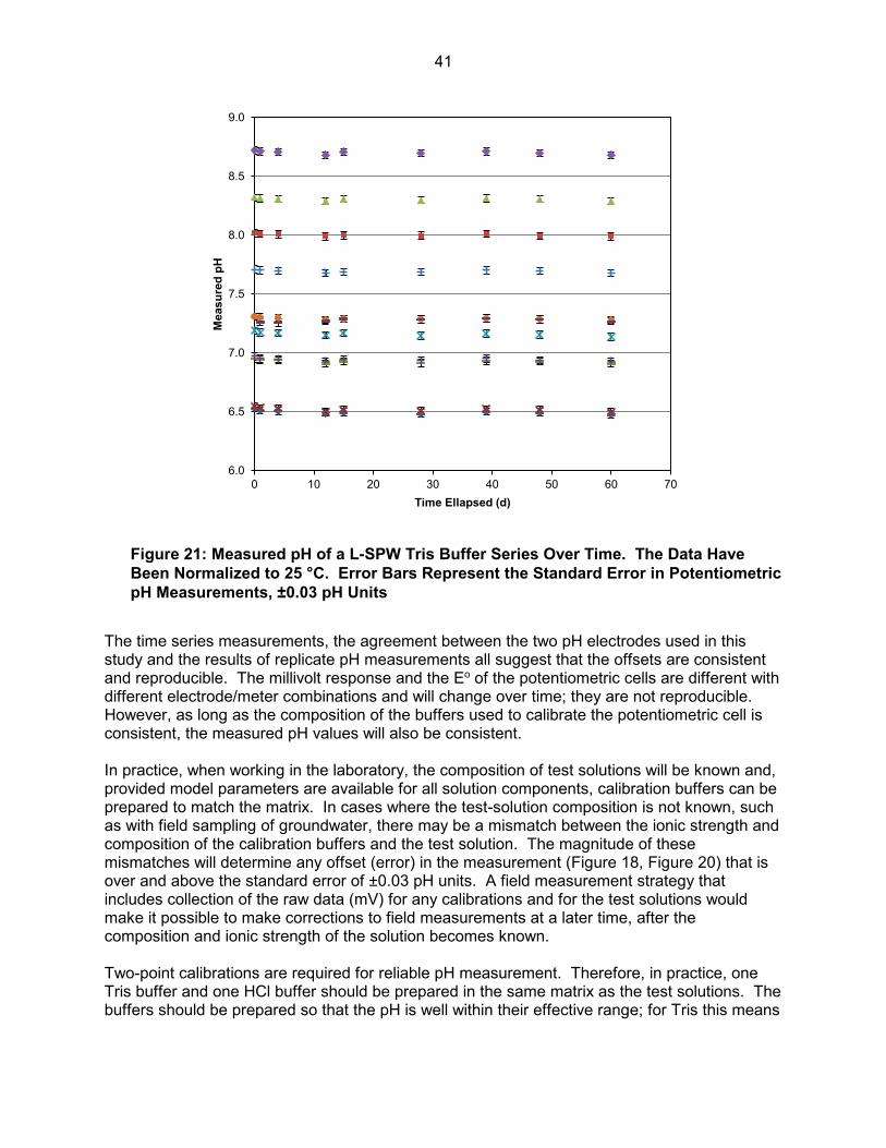
41

6.0

6.5

7.0

7.5

8.0

8.5

9.0

0 10 20 30 40 50 60 70

Mea

sure

d pH

Time Ellapsed (d)

Figure 21: Measured pH of a L-SPW Tris Buffer Series Over Time. The Data Have Been Normalized to 25 °C. Error Bars Represent the Standard Error in Potentiometric pH Measurements, ±0.03 pH Units

The time series measurements, the agreement between the two pH electrodes used in this study and the results of replicate pH measurements all suggest that the offsets are consistent and reproducible. The millivolt response and the Eo of the potentiometric cells are different with different electrode/meter combinations and will change over time; they are not reproducible. However, as long as the composition of the buffers used to calibrate the potentiometric cell is consistent, the measured pH values will also be consistent. In practice, when working in the laboratory, the composition of test solutions will be known and, provided model parameters are available for all solution components, calibration buffers can be prepared to match the matrix. In cases where the test-solution composition is not known, such as with field sampling of groundwater, there may be a mismatch between the ionic strength and composition of the calibration buffers and the test solution. The magnitude of these mismatches will determine any offset (error) in the measurement (Figure 18, Figure 20) that is over and above the standard error of ±0.03 pH units. A field measurement strategy that includes collection of the raw data (mV) for any calibrations and for the test solutions would make it possible to make corrections to field measurements at a later time, after the composition and ionic strength of the solution becomes known. Two-point calibrations are required for reliable pH measurement. Therefore, in practice, one Tris buffer and one HCl buffer should be prepared in the same matrix as the test solutions. The buffers should be prepared so that the pH is well within their effective range; for Tris this means

42

using Tris and TrisHCl salts at or near equal molar quantities. This would give, for example, a pH of 8.25 in S-SPW (Appendix B.4). The HCl buffer should have a pH <2.0.

5.3.2 Spectrophotometric pH Measurements The measured molar absorptivities for the phenol red indicator (Table 11) are not the same as those reported by Raghuraman et al. (2006b) because different wavelengths were used. Raghuraman et al. (2006b) used 445 nm and 570 nm wavelengths, and 431 nm and 559 nm wavelengths were used in this work. Furthermore, Raghuraman (2006b) used different instrumentation and it has also been reported that impurities in indicators, which can vary by manufacture and even by batch, can affect the molar absorptivities of the indicator and result in differences in measured pH by up to 0.01 unit (Yao et al. 2007). To put it in context, that magnitude of error from indicator impurities is similar to the magnitude of error associated with commercial NIST pH buffers. If required, the error from indicator impurities can be reduced by taking extra steps to purify each dye batch used (Liu et al. 2011), or molar absorptivities can be measured each time a new batch of indicator is used. The pK’a for phenol red in 0.1 mol/kg NaCl was recalculated at the wavelengths used by Raghuraman et al. (2006b) and with the molar absorptivities they reported. Raghuraman et al. (2006b) reported a pK’a of 7.79 at 20 °C and the corresponding pK’a measured in this study would be 7.74 at 25 °C. The uncertainty in the method developed by Raghuraman et al. (2006b) is ±0.1 unit. Therefore, the effect of differences in measured ε values between the studies is considered negligible.

Table 11: Measured Molar Absorptivities for Phenol Red in NaCl Solutions

0.05 mol/kg NaCl 1.0 mol/kg NaCl 5.0 mol/kg NaCl All Measurements

Mean σ Mean σ Mean σ Mean σ

ε559,B 59,975 279 59,170 1,477 55,823 583 58,323 2,039 ε559,A 74 29 -11 63 66 75 43 69 ε431,B 4,077 78 3,529 135 3,771 201 3,792 269 ε431,A 19,303 205 20,246 1,367 19,393 440 19,647 914

ε in units of (mol/kg)-1cm-1; σ is standard deviation The effect of equilibration with atmospheric CO2(g) on plots of log[B]/[A] versus modelled pH is presented in (Figure 22). The addition of CO2(g) adds a small degree of nonlinearity at the higher pH values, and this in-turn would contribute to error on the order of 0.02 to 0.03 in the pK’a measurement (intercept with the X axis). However, on the basis of arguments presented in Section 5.3.1, any effect from the presence of CO2(g) is expected to be negligible and all pK’a determinations were made with pH values obtained from the model without equilibrating with atmospheric CO2(g) (Appendix B.6).

43

y = 0.9968x - 7.6841R² = 0.9998

-0.8

-0.6

-0.4

-0.2

0.0

0.2

0.4

0.6

0.8

6.5 7.0 7.5 8.0 8.5

log

[B]/[

A]

pH

Figure 22: Plot of the Phenol Red Absorbance Ratio Versus pH in L-SPW. Filled Symbols Represent Modelled pH Assuming no Equilibrium with Atmospheric CO2(g); Hollow Symbols Represent Modelled pH with Solutions at Equilibrium with Atmospheric CO2(g) (log PCO2 = -3.4)

The pK’a of phenol red is sensitive to the ionic strength of the solution, but the data indicate that it is not sensitive to solution composition (Figure 23; Appendix B.6). With increasing ionic strength there is a rapid drop from the pK’a of 8.0 (Drummond et al. 1989) to a pK’a of 7.8 at 0.04 mol/kg. There is a minimum (pK’a = 7.6) in the ionic strength range of 1.0 to 2.5 mol/kg and then a gradual increase back to a pK’a of 7.8 at 8.2 mol/kg. This indicates that the maximum possible error in measured pH would be 0.2 units if the ionic strength of the test solution did not match the ionic strength of the buffer solutions. Therefore, the maximum error in pH measured spectrophotometrically is lower than that from potentiometric measurements (Section 5.3.1). Furthermore, there is an advantage in that the spectrophotometric measurements are not sensitive to variations in ionic composition. In this case, the difference in the measured pK’a for three solutions of similar ionic strength (~5.0 mol/kg) but different composition ranged from 0.01 to 0.04 (Figure 23). The useful range for the phenol red indicator is approximately ±1 pH unit from the pK’a value (Figure 22) and the measurement is therefore a function of ionic strength. The pH range for the spectrophotometric method in high-ionic-strength solutions could be extended by developing similar datasets for pK’a for multiple indicators that cover a broad pH range. Raghuraman (2006b) used a combination of colorimetric indicators in NaCl solutions, however NaCl buffer solutions limit the upper end of ionic strength to approximately 6 mol/kg. To extend the ionic strength range beyond 6 mol/kg requires the use of divalent cation salts, but this is only possible for a limited range of conditions because the Pitzer ion interaction parameters are not available to model pH for all buffers and for solutions with high Ca and Mg concentrations (Section 5.1, Figure 20). For DGR-related work it is desirable to have the ability to measure pH

44

in the range 4 to 9 and, until additional spectrophotometric datasets become available, the only available option is to use the potentiometric approach as outlined in Section 5.3.1.

7.4

7.5

7.6

7.7

7.8

7.9

8.0

8.1

8.2

8.3

8.4

0 1 2 3 4 5 6 7 8 9

Phen

ol R

ed p

K' a

Ionic Strength (mol/kg)

Infinite Dilution Reported Range

Just Tris

NaCl Series

L-SPW Series

S-SPW Series

Figure 23: Variation in Phenol Red pK'a with Ionic Strength and Solution Composition. Vertical Error Bars Represent 1σ. Horizontal Error Bars Represent the Standard Deviation in Ionic Strength Across a Tris Buffer Series; Where Not Visible, the Variation is Smaller than the Symbol

5.3.3 Uncertainty Assessment To evaluate what effect weighing errors could have had on the buffer pH, and therefore on the measured pK’a, a sensitivity analysis was conducted. The L-SPW2 buffer series was modelled for an additional 4 times considering:

• The maximum discrepancy that could occur if the actual mass of Tris and TrisHCl was in error by a factor of 5 times the precision of the balances used to weigh the Tris salts; and

• +5% and -5% of the molal values for the components of the L-SPW2 matrix (Na+, K+, Ca2+, Mg2+, Cl- and SO4

2-). The differences in both buffer pH and pK’a were apparent at the third decimal point, less than the resolution of the glass electrodes, ± 0.01 unit. The pK’a for phenol red in L-SPW2 ranged from 7.705 to 7.709 – a difference of 0.004 units. This is almost an order of magnitude smaller

45

than the standard deviation from replicate pK’a measurements, which was up to 0.03 units. Therefore, effects from possible errors in solution preparation are considered negligible.

5.4 SUMMARY Pitzer coefficients for two buffers, Tris and acetate, were added to the PHREEQC-Pitzer database and the model-calculated pK’a values were verified against literature data. The Pitzer coefficient data were more complete and considered more reliable for the Tris buffer – effective pH range of 6.5-9.0 – than for the acetate data – effective pH range of 3.0-5.6 units. pH buffers were also prepared using HCl. The Pitzer coefficients for the HCl system are well known and included in the standard PHREEQC-Pitzer database. It was decided to use Tris and HCl buffers to evaluate two methods for pH (-log aH) measurement in brine solutions: potentiometric measurements with glass electrodes, and spectrophotometric measurements using the colorimetric indicator phenol red (pKa = 8.0). The experiments involved a range of ionic strengths from 0.04 to 8.2 mol/kg, and solution compositions ranging from NaCl to the more complex S-SPW. Uncertainty in the modelled pH values for the buffer solutions increases for ionic strengths >6.0 mol/kg and for solutions that are more complex than just NaCl because Pitzer parameters for the Tris and acetate buffers have not been measured in such conditions. Extrapolation beyond these conditions could result in errors in modelled pH of up to 0.1 pH unit. The potentiometric pH electrode response is linear over a pH range from 1.4 to 9.1 and for ionic strengths up to 8.2 mol/kg. However, there is a systematic offset with increasing ionic strength such that an electrode calibrated with low ionic strength buffers will underestimate the pH of the highest ionic strength solution tested (8.2 mol/kg) by 0.6 to 0.7 pH units. For any given ionic strength, the potentiometric measurement is also sensitive to the ionic composition of the solution. Despite these effects, accurate potentiometric measurements are possible if the composition of the calibration buffers is similar to the test solution. The results of spectrophotometric measurements indicate that the stoichiometric disassociation constant (pK’a) of the phenol red indicator is sensitive to ionic strength but virtually insensitive to the composition of the solution. A maximum error of 0.2 units is possible for pH measured spectrophotometrically, if the ionic strength of the buffers does not match the ionic strength of the test solution. Because of the lower sensitivity of the spectrophotometric data to both ionic strength and solution composition, spectrophotometric measurements may prove more reliable than potentiometric measurements in unknown solutions, e.g., for pH measured in the field. However, the measurement range of phenol red is limited to pH ≈7-9. Additional indicators can be combined to increase the effective range of the spectrophotometric approach. The choice in additional indicators must be considered in the context of the availability and reliability of the appropriate Pitzer ion interaction coefficient data for the buffer as well as the logical combination of indicators to extract unique pH values from multi-indicator spectra (Raghuraman et al. 2006b). Both methods for pH measurement, potentiometric and spectrophotometric, can be adapted to reliably measure pH in high ionic strength solutions. The two methods offer distinct advantages and limitations. Therefore, the selection of which method to use will depend on the application.

46

6. CONCLUDING REMARKS A γ-RAD technique has been established for use in measurement of De and φI values for low-permeability sedimentary and crystalline rock samples. The γ-RAD method is free of beam-hardening artefacts and a linear calibration function is obtained that is essentially independent of background matrix. The γ-RAD method has been tested for measurement of porosity and diffusion coefficients of granite (<1% porosity; De = 3.1×10-13 m2/s) using an experimental design that allows for simultaneous TD (through-diffusion) measurements (De = 3.0×10-13 m2/s). Only one test has been conducted to date and the results of the two techniques are in good agreement, but there were problems identified in the TD experiment probably due to gradual occlusion of diffusion pathways by mineral-water reactions and the SNR (signal to noise ratio) is low for the γ-RAD measurements. These results demonstrate that the γ-RAD technique will be viable for crystalline rocks but further method development is required to demonstrate full confidence. A new method has been developed to generate partial gas saturation conditions in low-permeability rocks. The method is based on the relationship between gas solubility and pressure, whereby a rock sample that is initially 100% brine saturated is equilibrated with N2 gas at high pressure (up to 7000 kPa), and then the pressure is rapidly decreased to atmospheric pressure. This causes a corresponding decrease in gas solubility, resulting in exsolution of N2 to form gas bubbles in the pore spaces. The degree of partial saturation is determined by γ-RAD. During method development, the initial partial saturation work has been conducted on sandstone (13.0% porosity). Results of repeat experiments on the same sandstone sample display decrease in De values ranging from 21-56% for very similar degrees of partial saturation (15% and 13.5%, respectively). This is an unexpected result and it suggests that there is either an unidentified source of error in the measurements, or an effect from pore-scale variations in the distribution of the gas phase that cannot be resolved in the γ-RAD measurements. A preliminary result from Queenston Formation shale indicates a 53% decrease in De as a result of 14.6% partial gas saturation. This method shows great potential for evaluating the effect of partial saturation on diffusion in the Michigan Basin rocks that contain very high salinity porewater. However, these are challenging, multistep experiments and the technique requires further testing and development in order to gain full confidence in the results. Two techniques for measuring pH were evaluated – potentiometric and spectrophotometric pH measurement – in the context of high-ionic-strength brines. As part of the study, Pitzer coefficients for two buffers, Tris and acetate, were added to the PHREEQC-Pitzer database to calculate the pH of high-ionic-strength buffers. Using these buffers, it was found that the potentiometric measurement is sensitive to both the ionic strength and the ionic composition of the solution. Despite these effects, accurate potentiometric measurements are possible if the composition of the calibration buffers is similar to the test solution. The results of spectrophotometric measurements indicate that the association constant (pK’a) of the phenol red indicator is sensitive to ionic strength but virtually insensitive to the composition of the solution. The magnitude of the possible error in pH measurement using unmatched calibration buffers is larger for the potentiometric method than the spectrophotometric method. However, the range of pH that can be measured using the spectrophotometric method is limited by the narrow working range of the colorimetric indicators, whereas the potentiometric method is

47

applicable across the pH range. From this work, we have determined that both methods for pH measurement can be adapted to reliably measure pH in high ionic strength solutions. The two methods offer certain advantages and limitations. Therefore, the selection of which method to use will depend on the application. ACKNOWLEDGEMENTS We thank Professor Sean McGrady, Department of Chemistry, UNB, who provided access to a high-pressure chamber, and Sandra Riley for assisting with its operation.

48

REFERENCES Al, T., Y. Xiang and L. Cavé. 2010. Measurement of Diffusion Properties by X-ray Radiography

and by Through-Diffusion Techniques Using Iodide and Tritium Tracers: Core Samples from OS-1 and DGR-2. Intera Engineering Ltd., Technical Report TR-07-17 Revision 3. (Available at www.nwmo.ca)

Al, T., Y. Xiang, L. Cavé and D. Loomer. 2012. Measurement of Diffusion Properties by X-Ray

Radiography and by Through-Diffusion Techniques Using Iodide and Tritium Tracers: Core Samples from DGR-3 and DGR-4. Geofirma Engineering Ltd., Technical Report TR-08-27 Revision 2. (Available at www.nwmo.ca)

ANGUS Chemical Company. 2000. ANGUS Chemical Company Technology Review:

Biotechnology applications of Tris Amino® (Tris Buffer). TR 10, 12 p. AppliChem. 2008. Biological Buffers. A brochure providing information on biological buffers.

www.applichem.com. Bates, R.G. and J.B. Macaskill. 1985. Activity and osmotic coefficients of t-butylammonium

chloride; Activity coefficients of HCI in mixtures with Tris hydrochloride or t-butylammonium chloride at 25 ˚C. Journal of Solution Chemistry 14, 723-734.

Bates, R.G. and R.A. Robinson. 1974. An approach to conventional scales of ionic activity for

the standardization of ion-selective electrodes. Pure and Applied Chemistry 37, 573-577.

Bea, S.A., J. Carrera, C. Ayora, F. Batlle. 2010. Pitzer Algorithm: efficient implementation of

Pitzer equations in geochemical and reactive transport models. Computers & Geosciences 36, 526-538.

Bea Jofré, S.A., K.U. Mayer and K.T.B. MacQuarrie. 2011. Modelling Reactive Transport in

Sedimentary Rock Environments - Phase II MIN3P code enhancements and illustrative simulations for a glaciation scenario. Nuclear Waste Management Organization Report NWMO TR-2011-13. Toronto, Canada. (Available at www.nwmo.ca)

Buck, R.P., S. Rondinini, A.K. Covington, F.G.K. Bauke, C.M.A. Brett, M.F. Camoes, M.J.T.

Milton, T. Mussini, R. Naumann, K.W. Pratt, P. Spitzer and G.S. Wilson. 2002. Measurement of pH. Definition, standards, and procedures – IUPAC Recommendations 2002. Pure and Applied Chemistry 74, 2169-2200.

Cavé, L. and T. Al. 2006. Paleohydrogeology – Analytical TEM investigation of mineral

weathering in the Whiteshell research area. OPG Nuclear Waste Management Division, Report No: 06819-REP-01200-10156-R00.

Cavé, L., T. Al, Y. Xiang and P. Vilks. 2009. A technique for estimating one-dimensional

diffusion coefficients in low permeability sedimentary rock using X-ray radiography: Comparison with through-diffusion measurements. Journal of Contaminant Hydrology 103, 1-12.

http://www.nwmo.ca/

http://www.nwmo.ca/

http://www.applichem.com/

http://www.nwmo.ca/

49

Cavé, L., T. Al, Y. Xiang and D. Loomer. 2010. Investigations of Diffusive Transport Processes in Sedimentary Rock. Nuclear Waste Management Organization Report NWMO TR-2010-04. Toronto, Canada. (Available at www.nwmo.ca)

Covington, A.K. and M.I.A. Ferra. 1994. A Pitzer mixed electrolyte solution theory approach to

assignment of pH to standard buffer solutions. Journal of Solution Chemistry 23, 1-10. Dickson, A.G. 1984. pH scales and proton-transfer reactions in saline media such as sea water.

Geochimica et Cosmochimica Acta 48, 2299-2308. Dlugokencky, E. and P. Tans. 2014. Recent global monthly mean carbon dioxide

concentrations over marine surface sites. NOAA/ESRL (www.esrl.noaa.gov/gmd/ccgg/trends/).

Drummond, C.J., F. Grieser and T.W. Healy. 1989. Acid-base equilibria in aqueous micellar

solutions. Part 2: Sulphonephthalein indicators. Journal of the Chemical Society, Faraday Transactions 1 85, 537-550.

Foti, C., C. Rigano and S. Sammartano. 1999. Analysis of thermodynamic data for complex

formation: Protonation of tham and fluoride ion at different temperature and ionic strengths. Annali di Chimica 89, 87-98.

Gran, G. 1950. Determination of the equivalence point in potentiometric titrations. Acta

Chemica Scandinavica 4, 559-577. Gran, G. 1952. Determination of the equivalence point in potentiometric titrations. Part II.

Analyst 77, 661-671. Hansson, I. 1973. A new set of pH-scales and standard buffers for sea water. Deep-Sea

Research 20, 479-491. Harned, H.S. and B.B. Owen. 1958. The Physical Chemistry of Electrolytic Solutions, Reinhold,

New York, 803p. Hinds, G, P. Cooling, A. Wain, S. Zhou and A. Turnbill. 2009. Technical Note: Measurement of

pH in Concentrated Brines. Corrosion 65, 635-638. Hobbs, M., A. de Haller, M. Koroleva, M. Mazurek, J. Spangenberg, U. Mäder and D. Meier.

2011. Borehole DGR-3 and DGR-4 Porewater Investigations, R0. Geofirma Engineering Ltd. Technical Report TR-08-40, Toronto, Canada.

Hussein, E. M. A. 2011. Computer Radiation Imaging: Physics and Mathematics of Forward

and Inverse Problems, Elsevier, Amsterdam. Intera 2011. Descriptive Geosphere Site Model. Intera Engineering Ltd. report for the Nuclear

Waste Management Organization NWMO DGR-TR-2011-24 R000. Toronto, Canada. (available at www.nwmo.ca/dgrgeoscientificsitecharacterization)

Jensen, W.B. 2004. The symbol for pH. Journal of Chemical Education 81, 21.

http://www.nwmo.ca/

http://www.esrl.noaa.gov/gmd/ccgg/trends/

http://www.nwmo.ca/dgrgeoscientificsitecharacterization

50

Johansson, H., M. Siitari-Kauppi, M. Skalberg and E.L. Tullborg. 1998. Diffusion pathways in crystalline rock – examples from Aspo-diorite and fine-grained granite. Journal of Contaminant Hydrology 35, 41-53.

King, D.W. and D.R. Kester. 1989. Determination of seawater pH from 1.5 to 8.5 using

colorimetric indicators. Marine Chemistry 26, 5-20. Koroleva, M., A. de Haller, U. Mader, H.N. Waber and M. Mazurek. 2009. Borehole DGR-2:

Pore-water investigations. Intera Engineering Ltd., Technical Report TR-08-06, August 4, Institute of Geological Sciences, University of Bern, Switzerland.

Liu, X., M.C Patsavas and R.H. Byrne. 2011. Purification and characterization of meta-cresol

purple for spectrophotometric seawater pH measurements. Environmental Science & Technology 45, 4862-4868.

Loomer, D., Y. Xiang and T. Al. 2013a. Investigations of methods for quantifying diffusive

transport processes in sedimentary rock. Nuclear Waste Management Organization Report NWMO TR-2013-18. Toronto, Canada.

Loomer, D., L. Scott, T. Al, K.U. Mayer and S. Bea. 2013b. Diffusion–reaction studies in low

permeability shale using X-ray radiography with cesium. Applied Geochemistry 39, 49-58.

Loos, D., C. Pasel, M. Luckas, K.G. Schmidt and J.-D. Herbell. 2004. Experimental

investigation and modelling of the solubility of calcite and gypsum in aqueous systems at higher ionic strength. Fluid Phase Equilibria 219, 219-229.

MacInnes, D.A. 1919. The activities of the ions of strong electrolytes. Journal of the American

Chemical Society, 41, 1086-1092. Maksimov, I., M. Ohata, S. Nakamura, A. Hioki, K. Chiba and P. Spitzer. 2008. pH

determination on a carbonate buffer by Harned cells of different designs. Accreditation and Quality Assurance 13, 381-387.

Mao, S. and Z. Duan. 2006. A thermodynamic model for calculating nitrogen solubility, gas

phase composition and density of the N2-H2O-NaCl system. Liquid Phase Equilibria 248, 103-114.

Martz, T.R., J.J. Carr, C.R. French and M.D. DeGrandpre. 2003. A submersible autonomous

sensor for spectrophotometric pH measurements of natural waters. Analytical Chemistry 75, 1844-1850.

Mayer, K.U., E.O. Frind and D.W. Blowes. 2002. Multicomponent reactive transport modeling

in variably saturated porous media using a generalized formulation for kinetically controlled reactions. Water Resource Research 38, 1174, doi:10.1029/2001WR000862.

McFarland, W.N. and K.S. Norris. 1958. The control of pH by buffers in fish transport. California

Fish and Game 44, 4291.

51

Meinrath, G. 2002. Extended traceability of pH: an evaluation of the role of Pitzer’s equations. Analytical and Bioanalytical Chemistry, 374, 796-805.

MERK. 2014. The MERK Index, 14th Ed. Merck Sharp & Dohme Corp., a subsidiary of Merck &

Co., Inc., Whitehouse Station, NJ, USA. Mesmer, R.E., C. S. Patterson, R. H. Busey and H. F. Holmes. 1989. Ionization of acetic acid in

NaCl(aq) media: A potentiometric study to 573 K and 130 bar. The Journal of Physical Chemistry 93, 7483-7490.

Mesmer, R.E. and H.F. Holmes. 1992. pH, definition and measurement at high temperatures.

Journal of Solution Chemistry 21, 725-744. Millero, F.J., J.P. Hershey and M. Fernandez. 1987. The pK* of TRISH+ in Na-K-Mg-Ca-Cl-SO4

brines – pH scales. Geochimica et Cosmochimica Acta 51, 707-711. Millero, F.J., J.-Z. Zhang, S. Fiol, S. Sotolongo, R.N. Roy, K. Lee and S. Mane. 1993. The use

of buffers to measure the pH of seawater. Marine Chemistry 44, 143-152. Millero, F.J., B. DiTrolio, A.F. Suarez and G. Lando. 2009. Spectroscopic measurements of the

pH in NaCl brines. Geochimica et Cosmochimica Acta 73, 3109-3114. Mizera, J., A.H. Bond, G.R. Choppin and R.C. Moore. 1999. Dissociation constants of

carboxylic acids at high ionic strengths. In Actinide Speciation in High Ionic Strength Media: Experimental and Modeling Approaches to Predicting Actinide Speciation and Migration in the Subsurface, Reed, D.T.; Clark, S. B.; Linfeng R. (Eds.). Proceedings of an American Chemical Society Symposium, August 26-28, 1996, Orlando, Florida, Kluwer Academic/Plenum Publishers, New York, 113-124.

Mohan, C. 2006. Calbiochem®: A guide for the preparation and use of buffers in biological

systems, CB0052-2006 USD Buffers Booklet., EMD, San Diego, California. Nordstrom, D.K., C.N. Alpers, C.J. Ptacek and D. W. Blowes. 2000. Negative pH and extremely

acidic mine waters from Iron Mountain, California. Environmental Science & Technology 34, 254-258.

Novak, C.F., M. Borkowski and G.R. Choppin. 1996. Thermodynamic modeling of

Neptunium(V)-acetate complexation in concentrated NaCl media. Radiochimica Acta 74, 111-116.

Parkhurst, D.L. and C.A.J. Appelo. 1999. User’s Guide to PHREEQC (Version 2) – A

Computer Program for Speciation, Batch-Reaction, One-Dimensional Transport and Inverse Geochemical Calculations. Water-Resources Investigations Report 99-4259. U.S. Department of the Interior, U.S. Geological Survey, Denver, Colorado.

Parkhurst, D.L. and C.A.J. Appelo. 2013. Description of input and examples for PHREEQC

version 3 — A computer program for speciation, batch-reaction, one-dimensional transport, and inverse geochemical calculations. In: U.S. Geological Survey Techniques and Methods, book 6, chap. A43, 497 p., available online at http://pubs.usgs.gov/tm/06/a43.

http://pubs.usgs.gov/tm/06/a43

52

Pehrsson, L., F. Ingman and A. Johansson. 1976. Acid-base titrations by stepwise additions of

equal volumes of titrant with special reference to automatic titrations I: Theory, discussion of the Gran functions, the Hofstee method and two proposed methods for calculating equivalence volumes. Talanta 23, 769-780.

Plummer, L.N., D.L. Parkhurst, G.W. Fleming and S.A. Dunkle. 1988. A computer program

incorporating Pitzer’s equations for calculation of geochemical reactions in brines. USGS Water-Resources Investigations Report 88-4153, Reston, Virginia.

Pitzer, K.S. 1991. Ion interaction approach: theory and data correlation. In Activity Coefficients

in Electrolyte Solutions (2nd ed.), Pitzer, K.S. (ed). C.R.C. Press., Boca Raton, Florida, 542p.

Pitzer, K.S. and G. Mayorga. 1973. Thermodynamics of electrolytes. II. Activity and osmotic

coefficients for strong electrolytes with one or both ions univalent. The Journal of Physical Chemistry 77, 2300-2308.

Raghuraman, B., G. Gustavson, O. C. Mullins and P. Rabbito. 2006a. Spectroscopic pH

measurement for high temperatures, pressures and ionic strength. AIChE Journal 52, 3257-3265.

Raghuraman, B., G. Gustavson, R.E.G. van Hal, E. Dressaire and O. Zhdaneev. 2006b.

Extended-range spectroscopic pH measurement using optimized mixtures of dyes. Applied Spectroscopy 60, 1461-1469.

Reardon, E.J. and P.M. Moddle. 1985. Gas diffusion coefficient measurements on uranium mill

tailings: implications to cover layer design. Uranium 2, 111-131. Savoye, S., J. Page, C. Puente, C. Imbert and D. Coelho. 2010. New experimental approach for

studying diffusion through an intact and unsaturated medium: A case study with Callovo-Oxfordian argillite. Environmental Science and Technology 44, 3698–3704.

Siitari-Kauppi, M., A. Lindberg, K.H. Hellmuth, J. Timonen, K. Vaatainen, J. Hartikainen and K.

Hartikainen. 1997. The effect of microscale pore structure on matrix diffusion – a site-specific study on tonalite. Journal of Contaminant Hydrology 26, 147-158.

Skagius, K. and I. Neretnieks. 1986. Porosities and diffusivities of some nonsorbing species in

crystalline rocks. Water Resources Research 22, 389-398. Smith, S.W. 2003. The Scientist and Engineer’s Guide to Digital Signal Processing, California

Technical Publishing, San Diego. Spitzer, P., P. Fisicaro, G. Meinrath and D. Stoica. 2011. pH buffer assessment and Pitzer’s

equations. Accreditation and Quality Assurance 16, 191-198. Subudhi, R.K. 2009. A radiation transmission technique for the spatially-resolved

measurement of porosity and diffusion properties of porous media. M. Sc. Thesis, University of New Brunswick.

53

Subudhi, R.K., E.A. Hussein and T. Al. 2010. Measurement of spatial distribution of total and accessible porosity in sedimentary rocks using isotopic radiation transmission: Device design and testing. Applied Radiation and Isotopes 68, 496-504.

USGS. 2013. PHREEQC Interactive v. 3.0.6, June 2013.

http://wwwbrr.cr.usgs.gov/projects/GWC_coupled/phreeqc/. Vilks, P., J.J. Cramer, M. Jensen and N.H. Miller. 2003. In situ diffusion experiment in granite:

Phase I. Journal of Contaminant Hydrology 61, 191-202. Wall, D.E., N.A. Wall and L.H. Brush. 2006. Speciation and Solubility Modeling of Actinides in

the Waste Isolation Pilot Plant. In Separations for the Nuclear Fuel Cycle in the 21st Century, Chapter 20, 313–334. ACS Symposium Series 933.

Xiang, Y., T. Al, L. Scott and D. Loomer. 2013. Diffusive anisotropy in low-permeability

Ordovician sedimentary rocks from the Michigan Basin in southwest Ontario. Journal of Contaminant Hydrology 155, 31-45.

Xiang, Y. and T. Al. in prep. Effect of confining pressure on diffusion coefficients in low-

permeability Ordovician sedimentary rocks from the Michigan Basin in southwest Ontario. Manuscript in preparation.

Xu, S., A. Worman and B. Dverstorp. 2001. Heterogeneous matrix diffusion in crystalline rock

– implications for geosphere retardation of migrating radionuclides. Journal of Contaminant Hydrology 47, 365-378.

Yao, W., X. Liu and R. H. Byrne. 2007. Impurities in indicator used for spectrophotometric

seawater pH measurements: Assessment and remedies. Marine Chemistry 107, 167-172.

http://wwwbrr.cr.usgs.gov/projects/GWC_coupled/phreeqc/

55

APPENDIX A: METHOD FOR ENSURING 100% BRINE SATURATION

CONTENTS

Page A.1 SAMPLE DESCRIPTION............................................................................................... 57 A.1.1 Sandstones ................................................................................................................... 57 A.1.2 Queenston Formation Shale .......................................................................................... 57 A.2 IMPROVED EXPERIMENTAL PROCEDURES FOR ENSURING 100% BRINE SATURATION ............................................................................................................... 57 A.2.1 Sandstones ................................................................................................................... 58 A.2.2 Queenston Formation Shale .......................................................................................... 58 A.3 RESULTS ...................................................................................................................... 59

LIST OF TABLES Page

Table A.1: Water-Loss Porosity Data ....................................................................................... 59

LIST OF FIGURES Page

Figure A.1: Carbon Tan Sandstone Sample Partially Immersed in Water in a Vacuum Chamber: a) Immediately after Adding Water; and b) 30 min later ......................... 58

57

APPENDIX A: METHOD FOR ENSURING 100% BRINE SATURATION In conducting measurements of diffusion coefficients under partially brine-saturated conditions, the 100% brine-saturated condition represents a baseline against which all data will be compared. Saturation of a rock sample with a background brine solution is required for measurements of water-accessible porosity (φw) and De. The method for brine saturation used in previous work (Al et al. 2010, 2012; Cavé et al. 2009; Loomer et al. 2013b; Xiang et al. 2013; Xiang and Al, in prep.) involves submersing the sample in a brine solution followed by evacuation of the head space in a large (5 L) desiccator. This step is intended to remove the gas (air) initially present in the system, including dissolved air in the aqueous phase and trapped air in the rock pore spaces, and thereby maximize brine saturation of the sample. A.1 SAMPLE DESCRIPTION A.1.1 Sandstones Well characterized natural sandstone (Carbon Tan from Utah from Ohio) was purchased from Kocurek Industries, Inc. (Caldwell, TX). The porosities of the sandstone were reported to be 12.2-17.7% for Carbon Tan at purchase. They were used previously in our research lab as calibration matrices for the X-ray radiography method (Loomer et al. 2013a). The water-loss porosity measured at UNB was 12.8% for Carbon Tan , which is in the reported range. A.1.2 Queenston Formation Shale The Queenston Formation shale sample (DGR3-472) used in this study was prepared from a preserved core segment obtained during a drilling and coring program for characterization of the Deep Geologic Repository (DGR) site for low- and intermediate-level waste at the Bruce nuclear site near Tiverton, Ontario. Samples from the Queenston Formation are dominantly red-brown shale with minor green and grey shale. Clay minerals comprise 50-60% of these shales, 70-80% of which are illite and illite-smectite mixed layers. Chlorite is also present. Carbonates (calcite and dolomite, 30-40%) and quartz (approximately 10%) are the other major mineral components in these shales (Koroleva et al., 2009). The previously measured φw value for sample DGR3-472 was 8.6%. A.2 IMPROVED EXPERIMENTAL PROCEDURES FOR ENSURING 100% BRINE SATURATION Modification of the saturation procedure involves use of a smaller (approximately 100 mL) vacuum chamber to minimize water mass lost to evaporation (Figure A.1). Such a system allows the following two equilibria to be established and maintained.

1) Air(aq) ↔ Air(g, head space) 2) Air(g, rock pores) ↔ Air(aq)

If a vacuum is maintained in the headspace by removal of Air(g, head space) these coupled equilibria lead to removal of pore gas from the rock.

58

A.2.1 Sandstones The first step was to replace air in the rock pore space with a water soluble gas, CO2. Dry sandstone samples were placed in the vacuum chamber and the system was evacuated to approximately 90 kPa below atmospheric pressure (capacity of the pump) for an hour, after which CO2 gas was introduced and allowed to flow through the chamber for 10-20 min. The CO2 source was removed and the rock samples were allowed to equilibrate with the CO2 atmosphere for approximately 30 min. The chamber was then evacuated. This procedure of adding CO2 followed by evacuation of the chamber was repeated 3 times to ensure complete replacement of the air. After CO2 treatment, tap water was introduced into the chamber under vacuum to a level approximately 1/4 of the sample height (Figure A.1a), following which the chamber was evacuated. Within 30 minutes, the sandstone samples appeared wet as a result of capillary rise of water in the pores (Figure A.1b). Additional water was added under vacuum to completely submerge the samples, and then the system was allowed to sit in vacuum for 7 days. After water saturation, the φw values for the replicates of Carbon Tan sample were measured using the method outlined in Al et al. (2010, 2012) and Loomer et al. (2013a).

a) b)

Figure A.1: Carbon Tan Sandstone Sample Partially Immersed in Water in a Vacuum Chamber: a) Immediately after Adding Water; and b) 30 min Later

A.2.2 Queenston Formation Shale Triplicates of DGR3-472 were prepared from preserved drill cores. During the preparation it is expected that some water loss occurs from the surface of the samples. In order to resaturate them they were placed in the 100-mL vacuum chamber and the chamber was evacuated to approximately 90 kPa below atmospheric pressure for 1 hour. Shale synthetic porewater (S-SPW, Table 4) was introduced into the chamber under vacuum to reach approximately 1/4 of

59

the sample height. Partially immersed samples were allowed to sit in vacuum until samples were visibly wet – this commonly required 5-6 hours. Additional S-SPW was added under vacuum to submerse the samples completely. Submerged samples were allowed to sit in vacuum for 19 days, during which time the S-SPW solution was replaced 3-4 times with fresh solution to ensure constant concentration. After brine saturation, the φw values were measured using the method outlined in Al et al. (2010, 2012); Xiang and Al (in prep). A.3 RESULTS Measurements of φw, using this method are 9.0% for Queenston Formation shale, and 13.0% for Carbon Tan sandstone. Comparison of these values with those previously reported (Al et al. 2010, 2012; Loomer et al. 2013a; Xiang and Al, in prep.) indicates that the new porosity values are 2-4 % higher (Table A.1). The fact that the present results consistently display higher values suggests some improvement in the method of saturating samples.

Table A.1: Water-Loss Porosity Data

Sample ID DGR3-472 Carbon Tan Description Queenston shale Sandstone Method Refa This work Refb This work

Porosity, φw (%) 8.6 ± 0.1 9.0 ± 0.03 12.8 ± 0.2 13.0 ± 0.1

φw (Ref)/φw (This work) 0.96 0.98 a Xiang and Al, in prep.; b Loomer et al. 2013a.

61

APPENDIX B: PH MEASUREMENT IN BRINE SOLUTIONS

CONTENTS

Page B.1 MODIFIED PHREEQC-PITZER DATABASE ................................................................. 63 B.2 EXAMPLE PHREEQC INPUT FILE FOR pH BUFFER SOLUTIONS ............................ 79 B.3 EXAMPLE PHREEQC OUTPUT FILE FOR pH BUFFER SOLUTIONS ........................ 80 B.4 pH BUFFER SOLUTIONS ........................................................................................... 109 B.5 POTENTIOMETRIC pH MEASUREMENTS ................................................................ 118 B.6 PHENOL RED pK’a DETERMINATION RESULTS ...................................................... 129

63

B.1 MODIFIED PHREEQC-PITZER DATABASE The PHREEQC-PITZER database as modified at UNB (pitzerUNB.dat). “#” marks in front of an entry indicate that the entry is inactive (ignored) in the file. # PHREEQCI v.3.0.0-7430 PITZER database modified to include the Tris and Acetate buffer system and Cesium Pitzer parameters # Date: 22 March 2013 # Personnel: Diana Loomer (DL), UNB Fredericton # Parameter values listed after a "#" were considered and are included here for reference but the parameters (or combination of) # that resulted in the best fit and/or could be verified best are set as active in the file. # Data were verified with literature using "macinnes=false" which must be specified in input file. # The Pitzer parameters for TRISHCl and TRIS are only known at 25 °C(Millero 2009). # Millero et al. 1987 indicate reduced reliability in the Ca+2 and Mg+2 Pitzer parameters and/or that additional parameters # are required to fully define a solution with 1(or greater) mol/kg Ca or Mg. # For Millero's SO4 considerations, his calculations included using Harvie et al. 1984 values which are the same used in the # PHREEQC-Pitzer database. # Generally, Millero's data could be best reproduced for Tris and is considered the best for use. # Tishchenko 2000 determined several temp dependant Tris Pitzer parameters (included here) based on the same eqn PHREEQC # uses, but did not extend to the last 2 PHREEQC coefficients so PHREEQC would assume are zero. # Generally, it was found Novak's acetate data could be reproduced best for acetate. # # Using "analytic" instead of delta h for Tris pK temperature dependence # # Pitzer.DAT for calculating pressure dependence of reactions, with # molal volume of aqueous species and of minerals, and # critical temperatures and pressures of gases used in Peng-Robinson's EOS. # Details are given at the end of this file. SOLUTION_MASTER_SPECIES Tris Tris 1.0 121.138 121.138#DL Acetate Acetate- 1.0 59.045 59.045 #DL - From minteq.v4 Cs Cs+ 0.0 132.91 132.91 #DL H H+ -1. H 1.008 H(1) H+ -1. 0.0 E e- 0.0 0.0 0.0 O H2O 0.0 O 16.00 O(-2) H2O 0.0 0.0 Ca Ca+2 0.0 Ca 40.08 Mg Mg+2 0.0 Mg 24.305 Na Na+ 0.0 Na 22.9898 K K+ 0.0 K 39.0983 Fe Fe+2 0.0 Fe 55.847 Mn Mn+2 0.0 Mn 54.938 Ba Ba+2 0.0 Ba 137.33 Sr Sr+2 0.0 Sr 87.62 Cl Cl- 0.0 Cl 35.453 C CO3-2 2.0 HCO3 12.0111 C(4) CO3-2 2.0 HCO3 12.0111 Alkalinity CO3-2 1.0 Ca0.5(CO3)0.5 50.05 S SO4-2 0.0 SO4 32.064 S(6) SO4-2 0.0 SO4 B B(OH)3 0.0 B 10.81 Li Li+ 0.0 Li 6.941 Br Br- 0.0 Br 79.904 # redox-uncoupled gases Hdg Hdg 0 Hdg 2.016 # H2 gas Oxg Oxg 0 Oxg 32 # Oxygen gas Mtg Mtg 0.0 Mtg 16.032 # CH4 gas Sg H2Sg 1.0 H2Sg 34.08 Ntg Ntg 0 Ntg 28.0134 # N2 gas SOLUTION_SPECIES Tris = Tris #DL log_k 0.0 #DL Tris + H+ = (Tris)H+ #DL # log_k 8.075 #DL - zero ionic strength pKa @ 25 deg C - Bates and Hetzer 1961: J. Phys. Chem. 65.667-67 1 log_k 8.070 #DL - zero ionic stregth pKa @ 25 deg C - Foti et al. 1999: Ann. di Chim. 89, 87-98 (recommended value from compiled references)

64

# delta_h 11.377 kcal #DL - zero ionic strength delta h @ 25 deg C = 47,600 J/mol valid 0-50 deg C - Bates and Hetzer 1961: J. Phys. Chem. 65.667-67 1 delta_h 11.36 kcal #DL - zero ionic stregth pKa @ 25 deg C - Foti et al. 1999: Ann. di Chim. 89, 87-98 (recommended value from compiled references) # delta_h 11.395 kcal #DL - Tishchenko 2000 # -analytic 75.6853 0.0153422 -4884.31 -29.0765 Acetate- = Acetate- #DL - From minteq.v4 log_k 0.0 #DL - From minteq.v4 H+ + Acetate- = H(Acetate) #DL - acetic acid log_k 4.757 #DL - From minteq.v4 (zero ionic strength pKa for acetate/acetic acid (0.001m)) # log_k 4.756 #DL - From Handbook of Chemistry and Physics, 93rd Ed., 2012-2013 delta_h 0.098 kcal #DL - From minteq.v4 -gamma 0.0 0.0 #DL - From minteq.v4 (Debye-Hückel a, Debye-Hückel b coefficients - not relevant here) #DL - Id: 3309921 #DL - log K source: NIST46.4 #DL - Delta H source: NIST46.4 #DL - T and ionic strength: 0.00 25.0 # log_k 4.757 #DL - From Mesmer et al.: J. Phys. Chem. 1989, 93, 7483-7490(ionic strength 0 m NaCl; 25 deg C) # delta_h -0.12 kcal #DL - From Mesmer et al.: J. Phys. Chem. 1989, 93, 7483-7490(ionic strength 0 m NaCl; 25 deg C - different at different temperatures) Na+ + Acetate- = Na(Acetate) #DL - From minteq.v4 log_k -0.18 #DL - From minteq.v4 -0.18: corrected to zero ionic strength, if necessary. Original NIST database now discontinued delta_h 2.87 kcal #DL - From minteq.v4 #DL - Id: 5009920 #DL - log K source: NIST46.4 #DL - Delta H source: NIST46.4 #DL - T and ionic strength: 0.00 25.0 K+ + Acetate- = K(Acetate) #DL - From minteq.v4 log_k -0.1955 #DL - From minteq.v4 delta_h 1 kcal #DL - From minteq.v4 -gamma 0 0 #DL - From minteq.v4 #DL - Id: 4109921 #DL - log K source: NIST46.4 #DL - Delta H source: NIST46.2 #DL - T and ionic strength: 0.10 25.0 Ca+2 + Acetate- = Ca(Acetate)+ #DL - From minteq.v4 log_k 1.18 #DL - From minteq.v4 delta_h 0.96 kcal #DL - From minteq.v4 -gamma 0 0 #DL - From minteq.v4 #DL - Id: 1509920 #DL - log K source: NIST46.4 #DL - Delta H source: NIST46.4 #DL - T and ionic strength: 0.00 25.0 Mg+2 + Acetate- = Mg(Acetate)+ #DL - From minteq.v4 log_k 1.27 #DL - From minteq.v4 delta_h 0 kcal #DL - From minteq.v4 -gamma 0 0 #DL - From minteq.v4 #DL - Id: 4609920 #DL - log K source: NIST46.4 #DL - Delta H source: NIST46.2 #DL - T and ionic strength: 0.00 25.0 Cs+ = Cs+ #DL log_k 0.000 #DL -gamma 1.81 0.01 #DL - a,b parameters from Parkhurst 1990 cited in Langmuir 1997 p 133 H+ = H+ -dw 9.31e-9 e- = e- H2O = H2O Li+ = Li+ -dw 1.03e-9 -Vm -.0237 -.0690 11.5800 -2.7761 .4862 6 # supcrt Na+ = Na+ -dw 1.33e-9 -Vm 1.403 -2.285 4.419 -2.726 -5.125e-5 4.0 0.162 47.67 -3.09e-3 0.725 # supcrt modified # for calculating densities (rho) when I > 3... # -Vm 1.403 -2.285 4.419 -2.726 -5.125e-5 2.0 0.162 47.67 -3.09e-3 0.4 K+ = K+ -dw 1.96e-9

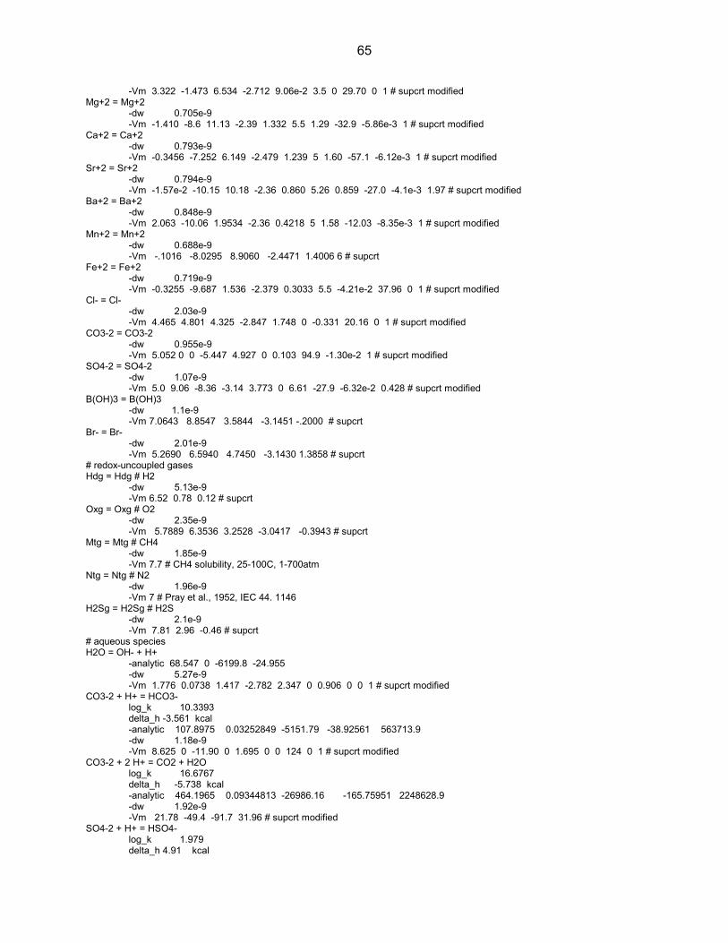
65

-Vm 3.322 -1.473 6.534 -2.712 9.06e-2 3.5 0 29.70 0 1 # supcrt modified Mg+2 = Mg+2 -dw 0.705e-9 -Vm -1.410 -8.6 11.13 -2.39 1.332 5.5 1.29 -32.9 -5.86e-3 1 # supcrt modified Ca+2 = Ca+2 -dw 0.793e-9 -Vm -0.3456 -7.252 6.149 -2.479 1.239 5 1.60 -57.1 -6.12e-3 1 # supcrt modified Sr+2 = Sr+2 -dw 0.794e-9 -Vm -1.57e-2 -10.15 10.18 -2.36 0.860 5.26 0.859 -27.0 -4.1e-3 1.97 # supcrt modified Ba+2 = Ba+2 -dw 0.848e-9 -Vm 2.063 -10.06 1.9534 -2.36 0.4218 5 1.58 -12.03 -8.35e-3 1 # supcrt modified Mn+2 = Mn+2 -dw 0.688e-9 -Vm -.1016 -8.0295 8.9060 -2.4471 1.4006 6 # supcrt Fe+2 = Fe+2 -dw 0.719e-9 -Vm -0.3255 -9.687 1.536 -2.379 0.3033 5.5 -4.21e-2 37.96 0 1 # supcrt modified Cl- = Cl- -dw 2.03e-9 -Vm 4.465 4.801 4.325 -2.847 1.748 0 -0.331 20.16 0 1 # supcrt modified CO3-2 = CO3-2 -dw 0.955e-9 -Vm 5.052 0 0 -5.447 4.927 0 0.103 94.9 -1.30e-2 1 # supcrt modified SO4-2 = SO4-2 -dw 1.07e-9 -Vm 5.0 9.06 -8.36 -3.14 3.773 0 6.61 -27.9 -6.32e-2 0.428 # supcrt modified B(OH)3 = B(OH)3 -dw 1.1e-9 -Vm 7.0643 8.8547 3.5844 -3.1451 -.2000 # supcrt Br- = Br- -dw 2.01e-9 -Vm 5.2690 6.5940 4.7450 -3.1430 1.3858 # supcrt # redox-uncoupled gases Hdg = Hdg # H2 -dw 5.13e-9 -Vm 6.52 0.78 0.12 # supcrt Oxg = Oxg # O2 -dw 2.35e-9 -Vm 5.7889 6.3536 3.2528 -3.0417 -0.3943 # supcrt Mtg = Mtg # CH4 -dw 1.85e-9 -Vm 7.7 # CH4 solubility, 25-100C, 1-700atm Ntg = Ntg # N2 -dw 1.96e-9 -Vm 7 # Pray et al., 1952, IEC 44. 1146 H2Sg = H2Sg # H2S -dw 2.1e-9 -Vm 7.81 2.96 -0.46 # supcrt # aqueous species H2O = OH- + H+ -analytic 68.547 0 -6199.8 -24.955 -dw 5.27e-9 -Vm 1.776 0.0738 1.417 -2.782 2.347 0 0.906 0 0 1 # supcrt modified CO3-2 + H+ = HCO3- log_k 10.3393 delta_h -3.561 kcal -analytic 107.8975 0.03252849 -5151.79 -38.92561 563713.9 -dw 1.18e-9 -Vm 8.625 0 -11.90 0 1.695 0 0 124 0 1 # supcrt modified CO3-2 + 2 H+ = CO2 + H2O log_k 16.6767 delta_h -5.738 kcal -analytic 464.1965 0.09344813 -26986.16 -165.75951 2248628.9 -dw 1.92e-9 -Vm 21.78 -49.4 -91.7 31.96 # supcrt modified SO4-2 + H+ = HSO4- log_k 1.979 delta_h 4.91 kcal

66

-analytic -5.3585 0.0183412 557.2461 -dw 1.33e-9 -Vm 8.2 9.2590 2.1108 -3.1618 1.1748 0 -0.3 15 0 1 # supcrt modified H2Sg = HSg- + H+ log_k -6.994 delta_h 5.30 kcal -analytical 11.17 -0.02386 -3279.0 -dw 2.1e-9 -Vm 5.0119 4.9799 3.4765 -2.9849 1.4410 # supcrt B(OH)3 + H2O = B(OH)4- + H+ log_k -9.239 delta_h 0 kcal 3B(OH)3 = B3O3(OH)4- + 2H2O + H+ log_k -7.528 delta_h 0 kcal 4B(OH)3 = B4O5(OH)4-2 + 3H2O + 2H+ log_k -16.134 delta_h 0 kcal Ca+2 + B(OH)3 + H2O = CaB(OH)4+ + H+ log_k -7.589 delta_h 0 kcal Mg+2 + B(OH)3 + H2O = MgB(OH)4+ + H+ log_k -7.840 delta_h 0 kcal #Ca+2 + CO3-2 = CaCO3 # log_k 3.151 # delta_h 3.547 kcal # -analytic -1228.806 -0.299440 35512.75 485.818 # -dw 4.46e-10 # complexes: calc'd with the Pikal formula # -Vm -.2430 -8.3748 9.0417 -2.4328 -.0300 # supcrt Mg+2 + H2O = MgOH+ + H+ log_k -11.809 delta_h 15.419 kcal Mg+2 + CO3-2 = MgCO3 log_k 2.928 delta_h 2.535 kcal -analytic -32.225 0.0 1093.486 12.72433 -dw 4.21e-10 -Vm -.5837 -9.2067 9.3687 -2.3984 -.0300 # supcrt PHASES CsCl #DL CsCl = Cs+ + Cl- #DL log_k 1.515 #DL - Hu et al 2007 CCPDTC 31:541-544 (note: they give solubility as ln Ksp, not log K - to convert: log K = ln K/2.303 = 3.488/2.303 = 1.515) CsBr #DL CsBr = Cs+ + Br- #DL log_k 0.817 #DL - Hu et al 2007 CCPDTC 31:541-544 (note: they give solubility as ln Ksp, not log K - to convert: log K = ln K/2.303 = 1.881/2.303 = 0.817) Anhydrite CaSO4 = Ca+2 + SO4-2 log_k -4.362 -anal 87.836 0 -3136.79 -32.953 # 50 - 160oC, 1 - 1e3 atm, anhydrite dissolution, Blount and Dickson, 1973, Am. Mineral. 58, 323. -Vm 46.1 # 136.14 / 2.95 Aragonite CaCO3 = CO3-2 + Ca+2 log_k -8.336 delta_h -2.589 kcal -analytic -171.8607 -.077993 2903.293 71.595 -Vm 34.04 Arcanite K2SO4 = + 1.0000 SO4-- + 2.0000 K+ log_k -1.776 -analytic 2.823 0.0 -1371.2 -Vm 65.5 Bischofite MgCl2:6H2O = + 1.0000 Mg++ + 2.0000 Cl- + 6.0000 H2O log_k 4.455 -analytic 3.524 0.0 277.6

67

Vm 127.1 Bloedite Na2Mg(SO4)2:4H2O = + 1.0000 Mg++ + 2.0000 Na+ + 2.0000 SO4-- + 4.0000 H2O log_k -2.347 -delta_H 0 # Not possible to calculate enthalpy of reaction Bloedite Vm 147 Brucite Mg(OH)2 = + 1.0000 Mg++ + 2.0000 OH- log_k -10.88 -delta_H 4.85 kcal/mol # -analytic -1.0280e+002 -1.9759e-002 9.0180e+003 3.8282e+001 1.4075e+002 # -Range: 0-300 Vm 24.6 Burkeite Na6CO3(SO4)2 = + 1.0000 CO3-2 + 2.0000 SO4-- + 6.0000 Na+ log_k -0.772 Vm 152 Calcite CaCO3 = CO3-2 + Ca+2 log_k -8.406 delta_h -2.297 kcal -analytic -171.8329 -0.077993 2839.319 71.595 -Vm 36.9 Carnallite KMgCl3:6H2O = K+ + Mg++ + 3Cl- + 6H2O log_k 4.330 Vm 173.7 Celestite SrSO4 = Sr+2 + SO4-2 log_k -6.630 -analytic -7.14 6.11E-03 75 0 0 -1.79E-05 # Howell et al., 1992, JCED 37, 464. -Vm 46.4 Dolomite CaMg(CO3)2 = Ca+2 + Mg+2 + 2 CO3-2 log_k -17.083 delta_h -9.436 kcal -Vm 64.5 Epsomite MgSO4:7H2O = Mg+2 + SO4-2 + 7 H2O log_k -1.881 -analytical 1.718 0.0 -1073. Vm 147 Gaylussite CaNa2(CO3)2:5H2O = Ca+2 + 2 CO3-2 + 2 Na+ + 5 H2O log_k -9.421 Glaserite NaK3(SO4)2 = Na+ + 3K+ + 2SO4-2 log_k -3.803 Glauberite Na2Ca(SO4)2 = Ca+2 + 2 Na+ + 2 SO4-2 log_k -5.245 Vm 99 Gypsum CaSO4:2H2O = Ca+2 + SO4-2 + 2 H2O log_k -4.581 delta_h -0.109 kcal -analytic 90.318 0.0 -4213. -32.641 -Vm 73.9 Barite BaSO4 = Ba+2 + SO4-2 log_k -9.97 delta_h 6.35 kcal -analytic 136.035 0.0 -7680.41 -48.595 -Vm 51.9 Halite NaCl = Cl- + Na+ log_k 1.570 -analytic -713.4616 -.1201241 37302.21 262.4583 -2106915. -Vm 27.1 Hexahydrite

68

MgSO4:6H2O = Mg+2 + SO4-2 + 6 H2O log_k -1.635 -analytic -62.666 0.0 1828. 22.187 Vm 132 Kainite KMgClSO4:3H2O = Cl- + K+ + Mg+2 + SO4-2 + 3 H2O log_k -0.193 Kalicinite KHCO3 = K+ + H+ + CO3-2 log_k -10.058 Kieserite MgSO4:H2O = Mg+2 + SO4-2 + H2O log_k -0.123 Vm 53.8 Labile_S Na4Ca(SO4)3:2H2O = 4Na+ + Ca+2 + 3SO4-2 + 2H2O log_k -5.672 Leonhardite MgSO4:4H2O = Mg+2 + SO4-2 + 4H2O log_k -0.887 Leonite K2Mg(SO4)2:4H2O = Mg+2 + 2 K+ + 2 SO4-2 + 4 H2O log_k -3.979 Magnesite MgCO3 = CO3-2 + Mg+2 log_k -7.834 delta_h -6.169 Vm 28.3 Mirabilite Na2SO4:10H2O = SO4-2 + 2 Na+ + 10 H2O log_k -1.214 -analytic -3862.234 -1.19856 93713.54 1577.756 0. Vm 216 Misenite K8H6(SO4)7 = 6 H+ + 7 SO4-2 + 8 K+ log_k -10.806 Nahcolite NaHCO3 = CO3-2 + H+ + Na+ log_k -10.742 Natron Na2CO3:10H2O = CO3-2 + 2 Na+ + 10.0000 H2O log_k -0.825 Nesquehonite MgCO3:3H2O = CO3-2 + Mg+2 + 3 H2O log_k -5.167 Pentahydrite MgSO4:5H2O = Mg+2 + SO4-2 + 5 H2O log_k -1.285 Pirssonite Na2Ca(CO3)2:2H2O = 2Na+ + Ca+2 + 2CO3-2 + 2 H2O log_k -9.234 Polyhalite K2MgCa2(SO4)4:2H2O = 2K+ + Mg+2 + 2 Ca+2 + 4SO4-2 + 2 H2O log_k -13.744 Vm 218 Portlandite Ca(OH)2 = Ca+2 + 2 OH- log_k -5.190 Schoenite K2Mg(SO4)2:6H2O = 2K+ + Mg+2 + 2 SO4-2 + 6H2O log_k -4.328 Sylvite KCl = K+ + Cl- log_k 0.900 -analytic 3.984 0.0 -919.55 Vm 37.5 Syngenite K2Ca(SO4)2:H2O = 2K+ + Ca+2 + 2SO4-2 + H2O log_k -7.448 Trona

69

Na3H(CO3)2:2H2O = 3 Na+ + H+ + 2CO3-2 + 2H2O log_k -11.384 Vm 106 Borax Na2(B4O5(OH)4):8H2O + 2 H+ = 4 B(OH)3 + 2 Na+ + 5 H2O log_k 12.464 Vm 223 Boric_acid,s B(OH)3 = B(OH)3 log_k -0.030 KB5O8:4H2O KB5O8:4H2O + 3H2O + H+ = 5B(OH)3 + K+ log_k 4.671 K2B4O7:4H2O K2B4O7:4H2O + H2O + 2H+ = 4B(OH)3 + 2K+ log_k 13.906 NaBO2:4H2O NaBO2:4H2O + H+ = B(OH)3 + Na+ + 3H2O log_k 9.568 NaB5O8:5H2O NaB5O8:5H2O + 2H2O + H+ = 5B(OH)3 + Na+ log_k 5.895 Teepleite Na2B(OH)4Cl + H+ = B(OH)3 + 2Na+ + Cl- + H2O log_k 10.840 CO2(g) CO2 = CO2 log_k -1.468 delta_h -4.776 kcal -analytic 119.87356 2.185434e-2 -7337.8 -44.7652 669371 -T_c 304.2 # critical T, K -P_c 72.80 # critical P, atm -Omega 0.225 # acentric factor H2O(g) H2O = H2O log_k 1.506; delta_h -44.03 kJ -T_c 647.3 # critical T, K -P_c 217.60 # critical P, atm -Omega 0.344 # acentric factor -analytic -16.5066 -2.0013E-3 2710.7 3.7646 0 2.24E-6 # redox-uncoupled gases Oxg(g) Oxg = Oxg -analytic -7.5001 7.8981e-003 0.0 0.0 2.0027e+005 T_c 154.6 ; -P_c 49.80 ; -Omega 0.021 Hdg(g) Hdg = Hdg -analytic -9.3114e+000 4.6473e-003 -4.9335e+001 1.4341e+000 1.2815e+005 -T_c 33.2 ; -P_c 12.80 ; -Omega 0.225 Ntg(g) Ntg = Ntg -analytic -58.453 1.81800E-03 3199 17.909 -27460 T_c 126.2 ; -P_c 33.50 ; -Omega 0.039 Mtg(g) Mtg = Mtg -analytic -2.4027e+001 4.7146e-003 3.7227e+002 6.4264e+000 2.3362e+005 T_c 190.6 ; -P_c 45.40 ; -Omega 0.008 H2Sg(g) H2Sg = H+ + HSg- -analytic -9.7354e+001 -3.1576e-002 1.8285e+003 3.7440e+001 2.8560e+001 T_c 373.2 ; -P_c 88.20 ; -Omega 0.1 PITZER -B0 (Tris)H+ Cl- 0.0395 #DL - Bates and Macaskill 1985: J. Solution Chem. 1985, 14, 723–734. (Tris)H+ SO4-2 0.09393 #DL - Bates and Macaskill 1986: J. Chem. Eng. Data 31, 416-418. # (Tris)H+ Cl- 0.03574 0 0 0.00013 #DL - Tishchenko 2000: Russ. Chem. Bull. 49, No 4, April, 2000 # H+ Cl- 0.17527 #DL - Bates and Macaskill 1985: J. Solution Chem. 14, 723–734 (Tris) # Na+ Cl- 0.075373 #DL - Manohar and Ananthaswamy 1991: CAN. J. CHEM. 69, 111-115 (acetate)

70

H+ OH- 0 #DL - not litsted, so same in PHREEQC Pitzer database, Novak et al 1996: Radiochimica Acta 74, 111-116 (acetate) H+ Acetate- 0 #DL - Novak et al 1996: Radiochimica Acta 74, 111-116 Na+ Acetate- 0.1426 #DL - Novak et al 1996: Radiochimica Acta 74, 111-116/Pitzer and Mayorga 1973: J. Phys. Chem. 77, 2300-2307/Pitzer 1991: Activity Coefficients in Electrolyte Solutions # Na+ Acetate- 0.13723 #DL - Manohar and Ananthaswamy 1991: CAN. J. CHEM. 69, 111-115 # K+ Acetate- 0.1587 #DL - Pitzer and Mayorga 1973: J. Phys. Chem. 77, 2300-2307/Pitzer 1991: Activity Coefficients in Electrolyte Solutions # K+ Acetate- 0.15343 #DL - (+/-0.00204)Marshall et al 1995: J. Chem. Eng. Data 40, 1041–1052 # K+ Acetate- 0.15283 #DL - Kim and Frederick 1988: J. Chem. Eng. Data 33, 177–184 # K+ Acetate- 0.161 #DL - Ferra et al 2011: J. Chem. Eng. Data 56, 3673–3678 # K+ Acetate- 0.228 #DL - DeRobertis et al (1999) J. Chem. Eng. Data 1999, 44, 262–270 K+ Acetate- 0.155 #DL - (+/-0.005)Spitzer et al 2011: Accred. Qual. Assur. 16, 191–198 Ca+2 Acetate- 0.269 #DL - Loos et al. 2004: Fluid Phase Equilibria 219, 219–229 # Ca+2 HCO3- -0.104 #DL - different than PHREEQC Pitzer database: Loos et al 2004: Fluid Phase Equilibria 219, 219–229 (acetate) # Ca+2 SO4-2 0.128 #DL - different in PHREEQC Pitzer database: Loos et al 2004: Fluid Phase Equilibria 219, 219–229 (acetate) Cs+ Cl- 0.030 #DL - Pitzer and Mayorga 1973: J Phys Chem 77, 2300-2307 Cs+ Br- 0.0279 #DL - Pitzer and Mayorga 1973: J Phys Chem 77, 2300-2307 Cs+ SO4-2 0.0888 #DL - Pitzer and Mayorga 1973: J Phys Chem 77, 2300-2307 Cs+ OH- 0.150 #DL - Pitzer and Mayorga 1973: J Phys Chem 77, 2300-2307 Na+ Cl- 0.0765 -777.03 -4.4706 0.008946 -3.3158E-6 K+ Cl- 0.04835 0 0 5.794E-4 Mg+2 Cl- 0.35235 0 0 -1.943E-4 Ca+2 Cl- 0.3159 0 0 -1.725E-4 MgOH+ Cl- -0.1 H+ Cl- 0.1775 0 0 -3.081E-4 Li+ Cl- 0.1494 0 0 -1.685E-4 Sr+2 Cl- 0.2858 0 0 0.717E-3 Fe+2 Cl- 0.335925 Mn+2 Cl- 0.327225 Ba+2 Cl- 0.2628 0 0 0.6405E-3 CaB(OH)4+ Cl- 0.12 MgB(OH)4+ Cl- 0.16 Na+ Br- 0.0973 0 0 7.692E-4 K+ Br- 0.0569 0 0 7.39E-4 H+ Br- 0.1960 0 0 -2.049E-4 Mg+2 Br- 0.4327 0 0 -5.625E-5 Ca+2 Br- 0.3816 0 0 -5.2275E-4 Li+ Br- 0.1748 0 0 -1.819E-4 Sr+2 Br- 0.331125 0 0 -0.32775E-3 Ba+2 Br- 0.31455 0 0 -0.33825E-3 Na+ SO4-2 0.01958 0 0 2.367E-3 K+ SO4-2 0.04995 0 0 1.44E-3 Mg+2 SO4-2 0.221 0 0 -0.69E-3 Ca+2 SO4-2 0.2 H+ SO4-2 0.0298 Li+ SO4-2 0.136275 0 0 0.5055E-3 Sr+2 SO4-2 0.200 0 0 -2.9E-3 Fe+2 SO4-2 0.2568 Mn+2 SO4-2 0.2065 Na+ HSO4- 0.0454 K+ HSO4- -0.0003 Mg+2 HSO4- 0.4746 Ca+2 HSO4- 0.2145 H+ HSO4- 0.2065 Fe+2 HSO4- 0.4273 Na+ OH- 0.0864 0 0 7.00E-4 K+ OH- 0.1298 Ca+2 OH- -0.1747 Li+ OH- 0.015 Ba+2 OH- 0.17175 Na+ HCO3- 0.0277 0 0 1.00E-3 K+ HCO3- 0.0296 0 0 0.996E-3 Mg+2 HCO3- 0.329 Ca+2 HCO3- 0.4 Sr+2 HCO3- 0.12 Na+ CO3-2 0.0399 0 0 1.79E-3 K+ CO3-2 0.1488 0 0 1.788E-3

71

Na+ B(OH)4- -0.0427 Na+ B3O3(OH)4- -0.056 Na+ B4O5(OH)4-2 -0.11 K+ B(OH)4- 0.035 K+ B3O3(OH)4- -0.13 K+ B4O5(OH)4-2 -0.022 -B1

(Tris)H+ Cl- 0.20978 #DL - Bates and Macaskill 1985: J. Solution Chem. 1985 14, 723–734. (Tris)H+ SO4-2 0.59829 #DL - Bates and Macaskill 1986: J. Chem. Eng. Data 31, 416-418.

# (Tris)H+ Cl- 0.21452 -5875.10 -36.291 0.05613 #DL - The A0 coeff is a different value in the temp dependance table than for the value listed at 25 deg C (0.21488), Tishchenko 2000 Russ.Chem.Bull. 49, No 4, April, 2000 # H+ Cl- 0.30197 #DL - Bates and Macaskill 1985: J. Solution Chem. 1985 14, 723–734 (Tris) # Na+ Cl- 0.277031 #DL - Manohar and Ananthaswamy 1991: CAN. J. CHEM. 69, 111-115 (acetate) H+ OH- 0 #DL - not listed, so same in PHREEQC Pitzer database, Novak et al 1996: Radiochimica Acta 74, 111-116 (acetate) H+ Acetate- 0 #DL - Novak et al 1996: Radiochimica Acta 74, 111-116/Mesmer et al 1989: J. Phys. Chem. 93, 7483-7490 # Na+ Acetate- 0.22 #DL - Novak et al 1996: Radiochimica Acta 74, 111-116/Mesmer et al 1989: J. Phys. Chem. 93, 7483-7490 Na+ Acetate- 0.3237 #DL - Pitzer and Mayorga 1973: J. Phys. Chem. 77, 2300-2307/Pitzer 1991: Activity Coefficients in Electrolyte Solutions # Na+ Acetate- 0.34915 #DL - Manohar and Ananthaswamy 1991: CAN. J. CHEM. 69, 111-115 # K+ Acetate- 0.3251 #DL - Pitzer and Mayorga 1973: J. Phys. Chem. 77, 2300-2307/Pitzer 1991: Activity Coefficients in Electrolyte Solutions # K+ Acetate- 0.34323 #DL - (+/-0.01102)Marshall et al 1995: J. Chem. Eng. Data 40, 1041–1052 # K+ Acetate- 0.35513 #DL - Kim and Frederick 1988: J. Chem. Eng. Data 33, 177–184 # K+ Acetate- 0.143 #DL - DeRobertis et al 1999: J. Chem. Eng. Data 44, 262–270 # K+ Acetate- 0.342 #DL - Ferra et al 2011: J. Chem. Eng. Data 56, 3673–3678 K+ Acetate- 0.3 #DL - Spitzer et al 2011: Accred. Qual. Assur. 16, 191–198 Ca+2 Acetate- 1.134 #DL - Loos et al 2004: Fluid Phase Equilibria 219, 219–229 # Ca+2 HCO3- 1.68 #DL - different in PHREEQC Pitzer database: Loos et al 2004: Fluid Phase Equilibria 219, 219–229 (acetate) # Ca+2 SO4-2 2.76 #DL - different in PHREEQC Pitzer database: Loos et al 2004: Fluid Phase Equilibria 219, 219–229 (acetate) Cs+ Cl- 0.0558 #DL - Pitzer and Mayorga 1973: J. Phys. Chem. 77, 2300-2307 Cs+ Br- 0.0139 #DL - Pitzer and Mayorga 1973: J. Phys. Chem. 77, 2300-2307 Cs+ SO4-2 1.11075 #DL - Pitzer and Mayorga 1973: J. Phys. Chem. 77, 2300-2307 Cs+ OH- 0.30 #DL - Pitzer and Mayorga 1973: J. Phys. Chem. 77, 2300-2307 Na+ Cl- 0.2664 0 0 6.1608E-5 1.0715E-6 K+ Cl- 0.2122 0 0 10.71E-4 Mg+2 Cl- 1.6815 0 0 3.6525E-3 Ca+2 Cl- 1.614 0 0 3.9E-3 MgOH+ Cl- 1.658 H+ Cl- 0.2945 0 0 1.419E-4 Li+ Cl- 0.3074 0 0 5.366E-4 Sr+2 Cl- 1.667 0 0 2.8425E-3 Fe+2 Cl- 1.53225 Mn+2 Cl- 1.55025 Ba+2 Cl- 1.49625 0 0 3.2325E-3 Na+ Br- 0.2791 0 0 10.79E-4 K+ Br- 0.2212 0 0 17.40E-4 H+ Br- 0.3564 0 0 4.467E-4 Mg+2 Br- 1.753 0 0 3.8625E-3 Ca+2 Br- 1.613 0 0 6.0375E-3 Li+ Br- 0.2547 0 0 6.636E-4 Sr+2 Br- 1.7115 0 0 6.5325E-3 Ba+2 Br- 1.56975 0 0 6.78E-3 Na+ SO4-2 1.113 0 0 5.6325E-3 K+ SO4-2 0.7793 0 0 6.6975E-3 Mg+2 SO4-2 3.343 0 0 1.53E-2 Ca+2 SO4-2 3.1973 0 0 5.46E-2 Li+ SO4-2 1.2705 0 0 1.41E-3 Sr+2 SO4-2 3.1973 0 0 27.0E-3 Fe+2 SO4-2 3.063 Mn+2 SO4-2 2.9511 Na+ HSO4- 0.398 K+ HSO4- 0.1735 Mg+2 HSO4- 1.729 Ca+2 HSO4- 2.53

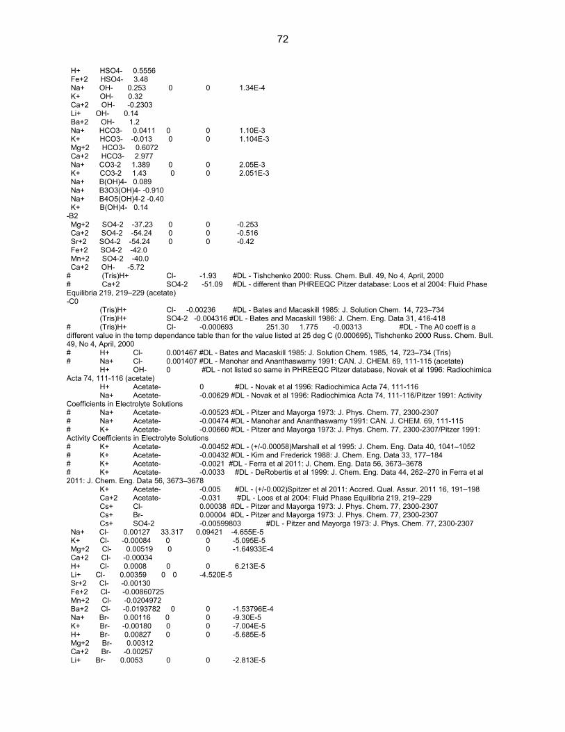
72

H+ HSO4- 0.5556 Fe+2 HSO4- 3.48 Na+ OH- 0.253 0 0 1.34E-4 K+ OH- 0.32 Ca+2 OH- -0.2303 Li+ OH- 0.14 Ba+2 OH- 1.2 Na+ HCO3- 0.0411 0 0 1.10E-3 K+ HCO3- -0.013 0 0 1.104E-3 Mg+2 HCO3- 0.6072 Ca+2 HCO3- 2.977 Na+ CO3-2 1.389 0 0 2.05E-3 K+ CO3-2 1.43 0 0 2.051E-3 Na+ B(OH)4- 0.089 Na+ B3O3(OH)4- -0.910 Na+ B4O5(OH)4-2 -0.40 K+ B(OH)4- 0.14 -B2 Mg+2 SO4-2 -37.23 0 0 -0.253 Ca+2 SO4-2 -54.24 0 0 -0.516 Sr+2 SO4-2 -54.24 0 0 -0.42 Fe+2 SO4-2 -42.0 Mn+2 SO4-2 -40.0 Ca+2 OH- -5.72 # (Tris)H+ Cl- -1.93 #DL - Tishchenko 2000: Russ. Chem. Bull. 49, No 4, April, 2000 # Ca+2 SO4-2 -51.09 #DL - different than PHREEQC Pitzer database: Loos et al 2004: Fluid Phase Equilibria 219, 219–229 (acetate) -C0 (Tris)H+ Cl- -0.00236 #DL - Bates and Macaskill 1985: J. Solution Chem. 14, 723–734 (Tris)H+ SO4-2 -0.004316 #DL - Bates and Macaskill 1986: J. Chem. Eng. Data 31, 416-418 # (Tris)H+ Cl- -0.000693 251.30 1.775 -0.00313 #DL - The A0 coeff is a different value in the temp dependance table than for the value listed at 25 deg C (0.000695), Tishchenko 2000 Russ. Chem. Bull. 49, No 4, April, 2000 # H+ Cl- 0.001467 #DL - Bates and Macaskill 1985: J. Solution Chem. 1985, 14, 723–734 (Tris) # Na+ Cl- 0.001407 #DL - Manohar and Ananthaswamy 1991: CAN. J. CHEM. 69, 111-115 (acetate) H+ OH- 0 #DL - not listed so same in PHREEQC Pitzer database, Novak et al 1996: Radiochimica Acta 74, 111-116 (acetate) H+ Acetate- 0 #DL - Novak et al 1996: Radiochimica Acta 74, 111-116 Na+ Acetate- -0.00629 #DL - Novak et al 1996: Radiochimica Acta 74, 111-116/Pitzer 1991: Activity Coefficients in Electrolyte Solutions # Na+ Acetate- -0.00523 #DL - Pitzer and Mayorga 1973: J. Phys. Chem. 77, 2300-2307 # Na+ Acetate- -0.00474 #DL - Manohar and Ananthaswamy 1991: CAN. J. CHEM. 69, 111-115 # K+ Acetate- -0.00660 #DL - Pitzer and Mayorga 1973: J. Phys. Chem. 77, 2300-2307/Pitzer 1991: Activity Coefficients in Electrolyte Solutions # K+ Acetate- -0.00452 #DL - (+/-0.00058)Marshall et al 1995: J. Chem. Eng. Data 40, 1041–1052 # K+ Acetate- -0.00432 #DL - Kim and Frederick 1988: J. Chem. Eng. Data 33, 177–184 # K+ Acetate- -0.0021 #DL - Ferra et al 2011: J. Chem. Eng. Data 56, 3673–3678 # K+ Acetate- -0.0033 #DL - DeRobertis et al 1999: J. Chem. Eng. Data 44, 262–270 in Ferra et al 2011: J. Chem. Eng. Data 56, 3673–3678 K+ Acetate- -0.005 #DL - (+/-0.002)Spitzer et al 2011: Accred. Qual. Assur. 2011 16, 191–198 Ca+2 Acetate- -0.031 #DL - Loos et al 2004: Fluid Phase Equilibria 219, 219–229 Cs+ Cl- 0.00038 #DL - Pitzer and Mayorga 1973: J. Phys. Chem. 77, 2300-2307 Cs+ Br- 0.00004 #DL - Pitzer and Mayorga 1973: J. Phys. Chem. 77, 2300-2307 Cs+ SO4-2 -0.00599803 #DL - Pitzer and Mayorga 1973: J. Phys. Chem. 77, 2300-2307 Na+ Cl- 0.00127 33.317 0.09421 -4.655E-5 K+ Cl- -0.00084 0 0 -5.095E-5 Mg+2 Cl- 0.00519 0 0 -1.64933E-4 Ca+2 Cl- -0.00034 H+ Cl- 0.0008 0 0 6.213E-5 Li+ Cl- 0.00359 0 0 -4.520E-5 Sr+2 Cl- -0.00130 Fe+2 Cl- -0.00860725 Mn+2 Cl- -0.0204972 Ba+2 Cl- -0.0193782 0 0 -1.53796E-4 Na+ Br- 0.00116 0 0 -9.30E-5 K+ Br- -0.00180 0 0 -7.004E-5 H+ Br- 0.00827 0 0 -5.685E-5 Mg+2 Br- 0.00312 Ca+2 Br- -0.00257 Li+ Br- 0.0053 0 0 -2.813E-5

73

Sr+2 Br- 0.00122506 Ba+2 Br- -0.0159576 Na+ SO4-2 0.00497 0 0 -4.87904E-4 Mg+2 SO4-2 0.025 0 0 0.523E-3 H+ SO4-2 0.0438 Li+ SO4-2 -0.00399338 0 0 -2.33345E-4 Fe+2 SO4-2 0.0209 Mn+2 SO4-2 0.01636 Na+ OH- 0.0044 0 0 -18.94E-5 K+ OH- 0.0041 K+ HCO3- -0.008 Na+ CO3-2 0.0044 K+ CO3-2 -0.0015 Na+ B(OH)4- 0.0114 -THETA # H+ Na+ 0.0289 #DL - Different than PHREEQC Pitzer database: used in Millero 2009 - ref Campell et al 1993: Mar. Chem. 44, 221–234: (0.0342-0.000209*25degC =0.0290)(Tris) (Tris)H+ H+ 0.0027 #DL - Bates and Macaskill 1985: J. Solution Chem. 14, 723–734. Can't tell is higher-order electrostatic terms were considered, but is from same paper as B and C values # (Tris)H+ Na+ -0.00055 -17353.52 -118.9707 0.2031 #DL - The A0 coeff is a different value in the temp dependance table than for the value listed at 25 deg C (-0.00086), Tishchenko 2000 Russ. Chem. Bull. 49, No 4, April, 2000 Acetate- Cl- -0.09 #DL - Novak et al 1996: Radiochimica Acta 74, 111-116 # Acetate- Cl- -0.00545 #DL - Manohar and Ananthaswamy 1991: CAN. J. CHEM. 69, 111-115/Ferra et al 2011: J. Chem. Eng. Data 56, 3673–3678 OH- Acetate- 0 #DL - Novak et al 1996: Radiochimica Acta 74, 111-116 Na+ Cs+ -0.033 #DL - Pitzer and Kim 1974: J. Am. Chem. Soc. 96, 5701-5707 K+ Cs+ 0.0 #DL - Pitzer and Kim 1974: J. Am. Chem. Soc. 96, 5701-5707 H+ Cs+ -0.044 #DL - Pitzer and Kim 1974: J. Am. Chem. Soc. 96, 5701-5707 K+ Na+ -0.012 Mg+2 Na+ 0.07 Ca+2 Na+ 0.07 Sr+2 Na+ 0.051 H+ Na+ 0.036 Ca+2 K+ 0.032 H+ K+ 0.005 Ca+2 Mg+2 0.007 H+ Mg+2 0.1 H+ Ca+2 0.092 SO4-2 Cl- 0.02 HSO4- Cl- -0.006 OH- Cl- -0.05 HCO3- Cl- 0.03 CO3-2 Cl- -0.02 B(OH)4- Cl- -0.065 B3O3(OH)4- Cl- 0.12 B4O5(OH)4-2 Cl- 0.074 OH- Br- -0.065 OH- SO4-2 -0.013 HCO3- SO4-2 0.01 CO3-2 SO4-2 0.02 B(OH)4- SO4-2 -0.012 B3O3(OH)4- SO4-2 0.10 B4O5(OH)4-2 SO4-2 0.12 CO3-2 OH- 0.1 CO3-2 HCO3- -0.04 B3O3(OH)4- HCO3- -0.10 B4O5(OH)4-2 HCO3- -0.087 -LAMDA Tris Na+ 0.0239 #DL - Millero et al 1987: Geochim. Cosmochim. Acta 51, 707–711 Tris Cl- 0 #DL - Millero et al 1987: Geochim. Cosmochim. Acta 51, 707–711 Tris K+ 0.0262 #DL - Millero et al 1987: Geochim. Cosmochim. Acta 51, 707–711 Tris Mg+2 -0.0594 #DL - Lower reliability indicated, Millero et al 1987: Geochim. Cosmochim. Acta 51, 707–711 Tris Ca+2 -0.2327 #DL - Lower reliability indicated, Millero et al 1987: Geochim. Cosmochim. Acta 51, 707–711 # Tris Tris 0.02617 -1692.47 -10.151 0.01524 #DL - The A0 coeff is a different value in the temp dependance table than for the value listed at 25 deg C (0.02591), Tishchenko 2000: Russ. Chem. Bull. 49, No 4, April, 2000 # H+ H(Acetate) 0.08 #DL - Partanen 1998: Acta Chem. Scand. 52, 985-994

74

# Na+ H(Acetate) 0.087 #DL - Partanen 1998: Acta Chem. Scand. 52, 985-994 # Cl- H(Acetate) 0 #DL - Partanen 1998: Acta Chem. Scand. 52, 985-994 # Acetate- H(Acetate) -0.09 #DL - Partanen 1998: Acta Chem. Scand. 52, 985-994 # H(Acetate) H(Acetate) -0.06 #DL - Partanen 1998: Acta Chem. Scand. 52, 985-994 # K+ H(Acetate) 0.044 #DL - Partanen 1998: Acta Chem. Scand. 52, 985-994/Ferra et al 2011: J. Chem. Eng. Data 56, 3673–3678 # K+ H(Acetate) 0.094 #DL - DeRobertis et al 1999: J. Chem. Eng. Data 44, 262–270 in Ferra et al 2011: J. Chem. Eng. Data 56, 3673–3678 Na+ CO2 0.085 K+ CO2 0.051 Mg+2 CO2 0.183 Ca+2 CO2 0.183 Cl- CO2 -0.005 SO4-2 CO2 0.097 HSO4- CO2 -0.003 Na+ B(OH)3 -0.097 K+ B(OH)3 -0.14 Cl- B(OH)3 0.091 SO4-2 B(OH)3 0.018 B3O3(OH)4- B(OH)3 -0.20 -ZETA Tris Na+ Cl- 0 #DL - Millero et al 1987: Geochim. Cosmochim. Acta 51, 707–711 # Tris (Tris)H+ Cl- -0.02747 2899.40 20.379 -0.03546 #DL - The A0 coeff is a different value in the temp dependance table than for the value listed at 25 deg C (-0.02741), Tishchenko 2000: Russ. Chem. Bull. 49, No 4, April, 2000 # Tris Na+ Cl- 0.02067 2475.34 17.384 -0.03045 #DL - The A0 coeff is a different value in the temp dependance table than for the value listed at 25 deg C (0.02097), Tishchenko 2000: Russ. Chem. Bull. 49, No 4, April, 2000 H+ Cl- B(OH)3 -0.0102 Na+ SO4-2 B(OH)3 0.046 Na+ SO4-2 CO2 -0.015 -PSI # H+ Na+ Cl- 0.0002 #DL - Different than PHREEQC Pitzer database: used in Millero 2009 ref Campell et al. 1993: Mar. Chem. 44, 221–234: psi HNaCl = 0? (Tris) # H+ Na+ Cl- -0.004 #DL - as listed in PHREEQC Pitzer database: Millero 1983: Geochim. Cosmochimm. Acta 41, 2121-2129 (Tris) H+ (Tris)H+ Cl- -0.013 #DL - Bates and Macaskill 1985: J. Solution Chem. 14, 723–734. Can't tell if higher-order electrostatic terms were considered, but is from same paper as B and C values # Na+ (Tris)H+ Cl- -0.00095 3920.1 27.114 -0.04657 #DL - The A0 coeff is a different value in the temp dependance table than for the value listed at 25 deg C (-0.000405), Tishchenko 2000: Russ. Chem. Bull. 49, No 4, April, 2000 Na+ H+ OH- 0 #DL - not listed so same in PHREEQC Pitzer database, Novak et al 1996: Radiochimica Acta 74, 111-116 Na+ H+ Acetate- 0 # DL - Novak et al 1996: Radiochimica Acta 74, 111-116 Na+ Acetate- Cl- 0.01029 #DL - Novak et al 1996: Radiochimica Acta 74, 111-116 # Na+ Acetate- Cl- -0.00205#DL - Manohar and Ananthaswamy 1991: CAN. J. CHEM. 69, 111-115 H+ Acetate- Cl- 0 #DL - Novak et al 1996: Radiochimica Acta 74, 111-116 H+ Cl- OH- 0 #DL - not listed so same in PHREEQC Pitzer database, Novak et al 1996: Radiochimica Acta 74, 111-116 Na+ Cs+ Cl- -0.003 #DL - Pitzer and Kim 1974: J. Am. Chem. Soc. 96, 5701-5707 K+ Cs+ Cl- -0.0013 #DL - Pitzer and Kim 1974: J. Am. Chem. Soc. 96, 5701-5707 H+ Cs+ Cl- -0.019 #DL - Pitzer and Kim 1974: J. Am. Chem. Soc. 96, 5701-5707 Na+ K+ Cl- -0.0018 Na+ K+ Br- -0.0022 Na+ K+ SO4-2 -0.010 Na+ K+ HCO3- -0.003 Na+ K+ CO3-2 0.003 Na+ Ca+2 Cl- -0.007 Na+ Sr+2 Cl- -0.0021 Na+ Ca+2 SO4-2 -0.055 Na+ Mg+2 Cl- -0.012 Na+ Mg+2 SO4-2 -0.015 Na+ H+ Cl- -0.004 Na+ H+ Br- -0.012 Na+ H+ HSO4- -0.0129 K+ Ca+2 Cl- -0.025 K+ Mg+2 Cl- -0.022 K+ Mg+2 SO4-2 -0.048 K+ H+ Cl- -0.011 K+ H+ Br- -0.021

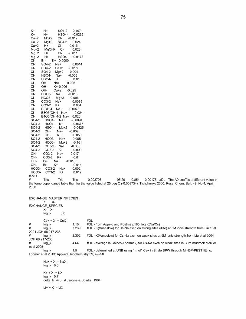
75

K+ H+ SO4-2 0.197 K+ H+ HSO4- -0.0265 Ca+2 Mg+2 Cl- -0.012 Ca+2 Mg+2 SO4-2 0.024 Ca+2 H+ Cl- -0.015 Mg+2 MgOH+ Cl- 0.028 Mg+2 H+ Cl- -0.011 Mg+2 H+ HSO4- -0.0178 Cl- Br- K+ 0.0000 Cl- SO4-2 Na+ 0.0014 Cl- SO4-2 Ca+2 -0.018 Cl- SO4-2 Mg+2 -0.004 Cl- HSO4- Na+ -0.006 Cl- HSO4- H+ 0.013 Cl- OH- Na+ -0.006 Cl- OH- K+ -0.006 Cl- OH- Ca+2 -0.025 Cl- HCO3- Na+ -0.015 Cl- HCO3- Mg+2 -0.096 Cl- CO3-2 Na+ 0.0085 Cl- CO3-2 K+ 0.004 Cl- B(OH)4- Na+ -0.0073 Cl- B3O3(OH)4- Na+ -0.024 Cl- B4O5(OH)4-2 Na+ 0.026 SO4-2 HSO4- Na+ -0.0094 SO4-2 HSO4- K+ -0.0677 SO4-2 HSO4- Mg+2 -0.0425 SO4-2 OH- Na+ -0.009 SO4-2 OH- K+ -0.050 SO4-2 HCO3- Na+ -0.005 SO4-2 HCO3- Mg+2 -0.161 SO4-2 CO3-2 Na+ -0.005 SO4-2 CO3-2 K+ -0.009 OH- CO3-2 Na+ -0.017 OH- CO3-2 K+ -0.01 OH- Br- Na+ -0.018 OH- Br- K+ -0.014 HCO3- CO3-2 Na+ 0.002 HCO3- CO3-2 K+ 0.012 #-MU # Tris Tris Tris -0.003707 -95.29 -0.854 0.00175 #DL - The A0 coeff is a different value in the temp dependance table than for the value listed at 25 deg C (-0.003734), Tishchenko 2000: Russ. Chem. Bull. 49, No 4, April, 2000 EXCHANGE_MASTER_SPECIES X X- EXCHANGE_SPECIES X- = X- log_k 0.0 Cs+ + X- = CsX #DL # log_k 1.10 #DL - from Appelo and Postma p160, log K(Na/Cs) # log_k 7.239 #DL - K(Vaneslow) for Cs-Na exch on strong sites (illite) at 5M ionic strength from Liu et al 2004 JCH 68 217-238 # log_k 2.302 #DL - K(Vaneslow) for Cs-Na exch on weak sites at 5M ionic strength from Liu et al 2004 JCH 68 217-238 # log_k 4.64 #DL - average K(Gaines-Thomas?) for Cs-Na exch on weak sites in Bure mudrock Melkior et al 2005 log_k 1.5 #DL - determined at UNB using 1 mol/l Cs+ in Shale SPW through MIN3P-PEST fitting, Loomer et al 2013: Applied Geochemistry 39, 49–58 Na+ + X- = NaX log_k 0.0 K+ + X- = KX log_k 0.7 delta_h -4.3 # Jardine & Sparks, 1984 Li+ + X- = LiX

76

log_k -0.08 delta_h 1.4 # Merriam & Thomas, 1956 Ca+2 + 2X- = CaX2 log_k 0.8 delta_h 7.2 # Van Bladel & Gheyl, 1980 Mg+2 + 2X- = MgX2 log_k 0.6 delta_h 7.4 # Laudelout et al., 1968 Sr+2 + 2X- = SrX2 log_k 0.91 delta_h 5.5 # Laudelout et al., 1968 Ba+2 + 2X- = BaX2 log_k 0.91 delta_h 4.5 # Laudelout et al., 1968 Mn+2 + 2X- = MnX2 log_k 0.52 Fe+2 + 2X- = FeX2 log_k 0.44 SURFACE_MASTER_SPECIES Hfo_s Hfo_sOH Hfo_w Hfo_wOH SURFACE_SPECIES # All surface data from # Dzombak and Morel, 1990 # # # Acid-base data from table 5.7 # # strong binding site--Hfo_s, Hfo_sOH = Hfo_sOH log_k 0.0 Hfo_sOH + H+ = Hfo_sOH2+ log_k 7.29 # = pKa1,int Hfo_sOH = Hfo_sO- + H+ log_k -8.93 # = -pKa2,int # weak binding site--Hfo_w Hfo_wOH = Hfo_wOH log_k 0.0 Hfo_wOH + H+ = Hfo_wOH2+ log_k 7.29 # = pKa1,int Hfo_wOH = Hfo_wO- + H+ log_k -8.93 # = -pKa2,int ############################################### # CATIONS # ############################################### # # Cations from table 10.1 or 10.5 # # Calcium Hfo_sOH + Ca+2 = Hfo_sOHCa+2 log_k 4.97 Hfo_wOH + Ca+2 = Hfo_wOCa+ + H+ log_k -5.85 # Strontium

77

Hfo_sOH + Sr+2 = Hfo_sOHSr+2 log_k 5.01 Hfo_wOH + Sr+2 = Hfo_wOSr+ + H+ log_k -6.58 Hfo_wOH + Sr+2 + H2O = Hfo_wOSrOH + 2H+ log_k -17.60 # Barium Hfo_sOH + Ba+2 = Hfo_sOHBa+2 log_k 5.46 Hfo_wOH + Ba+2 = Hfo_wOBa+ + H+ log_k -7.2 # table 10.5 # # Derived constants table 10.5 # # Magnesium Hfo_wOH + Mg+2 = Hfo_wOMg+ + H+ log_k -4.6 # Manganese Hfo_sOH + Mn+2 = Hfo_sOMn+ + H+ log_k -0.4 # table 10.5 Hfo_wOH + Mn+2 = Hfo_wOMn+ + H+ log_k -3.5 # table 10.5 # Iron # Hfo_sOH + Fe+2 = Hfo_sOFe+ + H+ # log_k 0.7 # LFER using table 10.5 # Hfo_wOH + Fe+2 = Hfo_wOFe+ + H+ # log_k -2.5 # LFER using table 10.5 # Iron, strong site: Appelo, Van der Weiden, Tournassat & Charlet, subm. Hfo_sOH + Fe+2 = Hfo_sOFe+ + H+ log_k -0.95 # Iron, weak site: Liger et al., GCA 63, 2939, re-optimized for D&M Hfo_wOH + Fe+2 = Hfo_wOFe+ + H+ log_k -2.98 Hfo_wOH + Fe+2 + H2O = Hfo_wOFeOH + 2H+ log_k -11.55 ############################################### # ANIONS # ############################################### # # Anions from table 10.6 # # # Anions from table 10.7 # # Borate Hfo_wOH + B(OH)3 = Hfo_wH2BO3 + H2O log_k 0.62 # # Anions from table 10.8 # # Sulfate Hfo_wOH + SO4-2 + H+ = Hfo_wSO4- + H2O log_k 7.78 Hfo_wOH + SO4-2 = Hfo_wOHSO4-2 log_k 0.79 # # Carbonate: Van Geen et al., 1994 reoptimized for HFO # 0.15 g HFO/L has 0.344 mM sites == 2 g of Van Geen's Goethite/L # # Hfo_wOH + CO3-2 + H+ = Hfo_wCO3- + H2O # log_k 12.56

78

# # Hfo_wOH + CO3-2 + 2H+= Hfo_wHCO3 + H2O # log_k 20.62 END MEAN GAM CaCl2 CaSO4 CaCO3 Ca(OH)2 MgCl2 MgSO4 MgCO3 Mg(OH)2 NaCl Na2SO4 NaHCO3 Na2CO3 NaOH KCl K2SO4 KHCO3 K2CO3 KOH HCl H2SO4 HBr END # For the reaction aA + bB = cC + dD, # with delta_v = c*Vm(C) + d*Vm(D) - a*Vm(A) - b*Vm(B), # PHREEQC adds the pressure term to log_k: -= delta_v * (P - 1) / (2.3RT). # Vm(A) is volume of A, cm3/mol, P is pressure, atm, R is the gas constant, T is Kelvin. # Gas-pressures and fugacity coefficients are calculated with Peng-Robinson's EOS. # Binary interaction coefficients from Soreide and Whitson, 1992, FPE 77, 217 are # hard-coded in calc_PR(): # kij CH4 CO2 H2S N2 # H2O 0.49 0.19 0.19 0.49 # ============================================================================================= # The molar volumes of solids are entered with # -Vm vm cm3/mol # vm is the molar volume, cm3/mol (default), but dm3/mol and m3/mol are permitted. # Data for minerals' vm (= MW (g/mol) / rho (g/cm3)) are defined using rho from # Deer, Howie and Zussman, The rock-forming minerals, Longman. # -------------------- # Temperature- and pressure-dependent volumina of aqueous species are calculated with a Redlich- # type equation (cf. Redlich and Meyer, Chem. Rev. 64, 221), from parameters entered with # -Vm a1 a2 a3 a4 W a0 i1 i2 i3 i4 # The volume (cm3/mol) is # Vm(T, pb, I) = 41.84 * (a1 * 0.1 + a2 * 100 / (2600 + pb) + a3 / (T - 228) + # a4 * 1e4 / (2600 + pb) / (T - 228) - W * QBrn) # + z^2 / 2 * Av * f(I^0.5) # + (i1 + i2 / (T - 228) + i3 * (T - 228)) * I^i4 # Volumina at I = 0 are obtained using supcrt92 formulas (Johnson et al., 1992, CG 18, 899). # 41.84 transforms cal/bar/mol into cm3/mol. # pb is pressure in bar. # W * QBrn is the Born volume, calculated from Wref and the pressure dependence of the # dielectric constant of water (f(P, T), see below). # z is charge of the solute species. # Av is the Debye-Hueckel limiting slope. # a0 is the ion-size parameter in the extended Debye-Hueckel paramter: # f(I^0.5) = I^0.5) / (1 + a0 * DH_B * I^0.5), # a0 = -gamma x for cations, = 0 for anions. # Av (P, T) is calculated using the dielectric constant of water from Bradley and Pitzer, 1979, JPC 83, 1599, # and the compressibility of pure water. # The density of pure water at water saturation pressure is calculated with eqn 2.6 from # Wagner and Pruss, 2002, J. Phys. Chem. Ref. Data 31, 387. At higher P,T with polynomials # interpolated from IAPWS table 3 (2007).

79

# # Data for species' parameters, commented with ‘# supcrt modified’, were fitted from data # compiled by Laliberte, 2009, J. Chem. Eng. Data 54, 1725, + additions, see Appelo, Parkhurst and Post (in prep.) # H+ has the reference volume of 0 at all P, T and I. # For Cl-, parameters were obtained from densities of HCl solutions up to 176 oC, 1 - 280 atm. # The numbers for cations were extracted from the densities of cation-Cl-solutions. # Other anions and OH- then follow from the measured densities of cation-anion solutions. # Water dissociation was fitted from Bandura and Lvov, 2006, J. Phys. Chem. Ref. Data, 35, 15, 0-200 oC, 1-2000 atm. # -------------------- # If -Vm is not defined, the a-f values from -Millero a b c d e f (if available) will be used for calculating # Vm(t, I) = a + b * t + c * t^2 + z^2 / 2 * Av * I^0.5 + (d + e * t + f * t^2) * I # t is temperature in oC. # # redox-uncoupled gases have been added for H2 (Hdg), O2 (Oxg), CH4 (Mtg), N2 (Ntg), # H2S (H2Sg, species HSg-, etc.). # # ============================================================================================= # It remains the responsibility of the user to check the calculated results, for example with # measured solubilities as a function of (P, T). B.2 EXAMPLE PHREEQC INPUT FILE FOR pH BUFFER SOLUTIONS TITLE Tris Buffer solutions (ionic strength 6 m) #Part of a series of L-SPW based solutions to cover a large range of ionic strengths SELECTED_OUTPUT -file 12xLSPWBuffersAsMade20131203.csv -reset false -solution true -ionic_strength true -percent_error true -pH true -totals Na K Ca Mg Cl S(6) Tris -saturation_indices halite gypsum END PITZER -macinnes false SOLUTION_SPREAD -pe 11 -units mol/kgw Number Na K Ca Mg Cl S(6) Tris pH charge 1 2.64240 0.59453 0.62866 0.26424 5.0775349 0.00110 0.0600 7.00000 2 2.64240 0.59453 0.62866 0.26424 5.0755069 0.00110 0.0600 7.00000 3 2.64240 0.59453 0.62866 0.26424 5.0725195 0.00110 0.0600 7.00000 4 2.64240 0.59453 0.62866 0.26424 5.0695803 0.00110 0.0601 7.00000 5 2.64240 0.59453 0.62866 0.26424 5.0655326 0.00110 0.0600 7.00000 6 2.64240 0.59453 0.62866 0.26424 5.0585272 0.00110 0.0600 7.00000 7 2.64240 0.59453 0.62866 0.26424 5.0505570 0.00110 0.0600 7.00000 Save Solution 1-7 END Solution 8 Just 1.2x's LSPW (no Tris) -pe 11 -units mol/L -pH 7 charge -density 1.17505 Na 2.40000 K 0.54000 Ca 0.5710 Mg 0.24000 Cl 4.56000

80

S(6) 0.00100 Save Solution 8 END USE solution 1 EQUILIBRIUM_PHASES 1 CO2(g) -3.4 10 END USE solution 2 EQUILIBRIUM_PHASES 2 CO2(g) -3.4 10 END USE solution 3 EQUILIBRIUM_PHASES 3 CO2(g) -3.4 10 END USE solution 4 EQUILIBRIUM_PHASES 4 CO2(g) -3.4 10 END USE solution 5 EQUILIBRIUM_PHASES 5 CO2(g) -3.4 10 END USE solution 6 EQUILIBRIUM_PHASES 6 CO2(g) -3.4 10 END USE solution 7 EQUILIBRIUM_PHASES 7 CO2(g) -3.4 10 END USE solution 8 EQUILIBRIUM_PHASES 8 CO2(g) -3.4 10 B.3 EXAMPLE PHREEQC OUTPUT FILE FOR pH BUFFER SOLUTIONS Input file: D:\NWMO\pH measurement\PRpKa\PHREEQC\12xLSPWBuffersAsMade20131203.pqi Output file: D:\NWMO\pH measurement\PRpKa\PHREEQC\12xLSPWBuffersAsMade20131203.pqo Database file: C:\Program Files\USGS\Phreeqc Interactive 3.0.0-7430\database\pitzerUNB.dat ------------------ Reading data base. ------------------ SOLUTION_MASTER_SPECIES SOLUTION_SPECIES PHASES PITZER EXCHANGE_MASTER_SPECIES EXCHANGE_SPECIES SURFACE_MASTER_SPECIES SURFACE_SPECIES END ------------------------------------ Reading input data for simulation 1. ------------------------------------

81

DATABASE C:\Program Files\USGS\Phreeqc Interactive 3.0.0-7430\database\pitzerUNB.dat TITLE Tris Buffer solutions (ionic strength 6 m) SELECTED_OUTPUT file 12xLSPWBuffersAsMade20131203.csv reset false solution true ionic_strength true percent_error true ph true totals Na K Ca Mg Cl S(6) Tris saturation_indices halite gypsum END ----- TITLE ----- Tris Buffer solutions (ionic strength 6 m) ------------------ End of simulation. ------------------ ------------------------------------ Reading input data for simulation 2. ------------------------------------ PITZER macinnes false SOLUTION_SPREAD pe 11 units mol/kgw Number Na K Ca Mg Cl S(6) Tris pH charge 1 2.64240 0.59453 0.62866 0.26424 5.0775349 0.00110 0.0600 7.00000 2 2.64240 0.59453 0.62866 0.26424 5.0755069 0.00110 0.0600 7.00000 3 2.64240 0.59453 0.62866 0.26424 5.0725195 0.00110 0.0600 7.00000 4 2.64240 0.59453 0.62866 0.26424 5.0695803 0.00110 0.0601 7.00000 5 2.64240 0.59453 0.62866 0.26424 5.0655326 0.00110 0.0600 7.00000 6 2.64240 0.59453 0.62866 0.26424 5.0585272 0.00110 0.0600 7.00000 7 2.64240 0.59453 0.62866 0.26424 5.0505570 0.00110 0.0600 7.00000 Save Solution 1-7 END ------------------------------------------- Beginning of initial solution calculations. ------------------------------------------- Initial solution 1. -----------------------------Solution composition------------------------------ Elements Molality Moles Ca 6.287e-001 6.287e-001 Cl 5.078e+000 5.078e+000 K 5.945e-001 5.945e-001 Mg 2.642e-001 2.642e-001 Na 2.642e+000 2.642e+000 S(6) 1.100e-003 1.100e-003 Tris 6.000e-002 6.000e-002 ----------------------------Description of solution---------------------------- pH = 7.087 Charge balance pe = 11.000 Specific Conductance (uS/cm, 25 oC) = 511867 Density (g/cm3) = 1.18218 Volume (L) = 1.10231 Activity of water = 0.808 Ionic strength = 5.974e+000 Mass of water (kg) = 1.000e+000 Total alkalinity (eq/kg) = 2.995e-003

82

Total carbon (mol/kg) = 0.000e+000 Total CO2 (mol/kg) = 0.000e+000 Temperature (deg C) = 25.00 Electrical balance (eq) = 7.034e-016 Percent error, 100*(Cat-|An|)/(Cat+|An|) = 0.00 Iterations = 12 Gamma iterations = 5 Osmotic coefficient = 1.27364 Density of water = 0.99704 Total H = 1.110695e+002 Total O = 5.551063e+001 ----------------------------Distribution of species---------------------------- Unscaled Unscaled Unscaled log log log Species Molality Activity Molality Activity Gamma cm3/mol OH- 3.968e-007 9.957e-008 -6.401 -7.002 -0.600 3.81 H+ 3.290e-008 8.180e-008 -7.483 -7.087 0.396 0.00 H2O 5.551e+001 8.084e-001 1.744 -0.092 0.000 18.07 Ca 6.287e-001 Ca+2 6.287e-001 3.118e-001 -0.202 -0.506 -0.305 -14.28 Cl 5.078e+000 Cl- 5.078e+000 5.850e+000 0.706 0.767 0.062 20.09 K 5.945e-001 K+ 5.945e-001 2.470e-001 -0.226 -0.607 -0.381 12.11 Mg 2.642e-001 Mg+2 2.642e-001 1.983e-001 -0.578 -0.703 -0.125 -17.78 MgOH+ 8.228e-006 3.042e-006 -5.085 -5.517 -0.432 (0) Na 2.642e+000 Na+ 2.642e+000 2.016e+000 0.422 0.304 -0.118 1.41 S(6) 1.100e-003 SO4-2 1.100e-003 2.412e-005 -2.959 -4.618 -1.659 26.83 HSO4- 2.131e-010 1.880e-010 -9.671 -9.726 -0.055 42.04 Tris 6.000e-002 (Tris)H+ 5.701e-002 2.430e-002 -1.244 -1.614 -0.370 (0) Tris 2.987e-003 2.528e-003 -2.525 -2.597 -0.072 (0) ------------------------------Saturation indices------------------------------- Phase SI log IAP log K(298 K, 1 atm) Anhydrite -0.90 -5.12 -4.22 CaSO4 Arcanite -4.06 -5.83 -1.78 K2SO4 Bischofite -4.18 0.28 4.46 MgCl2:6H2O Bloedite -7.35 -9.70 -2.35 Na2Mg(SO4)2:4H2O Brucite -3.83 -14.71 -10.88 Mg(OH)2 Carnallite -3.89 0.44 4.33 KMgCl3:6H2O Epsomite -4.09 -5.97 -1.88 MgSO4:7H2O Glaserite -6.95 -10.75 -3.80 NaK3(SO4)2 Glauberite -3.89 -9.13 -5.25 Na2Ca(SO4)2 Gypsum -0.73 -5.31 -4.58 CaSO4:2H2O H2O(g) -1.60 -0.09 1.50 H2O Halite -0.50 1.07 1.57 NaCl Hexahydrite -4.24 -5.87 -1.63 MgSO4:6H2O Kainite -5.24 -5.44 -0.19 KMgClSO4:3H2O Kieserite -5.29 -5.41 -0.12 MgSO4:H2O Labile_S -7.65 -13.33 -5.67 Na4Ca(SO4)3:2H2O Leonhardite -4.80 -5.69 -0.89 MgSO4:4H2O Leonite -7.54 -11.52 -3.98 K2Mg(SO4)2:4H2O Mirabilite -3.72 -4.93 -1.21 Na2SO4:10H2O Misenite -68.90 -79.71 -10.81 K8H6(SO4)7 Pentahydrite -4.50 -5.78 -1.28 MgSO4:5H2O Polyhalite -7.84 -21.58 -13.74 K2MgCa2(SO4)4:2H2O Portlandite -9.32 -14.51 -5.19 Ca(OH)2 Schoenite -7.38 -11.71 -4.33 K2Mg(SO4)2:6H2O Sylvite -0.74 0.16 0.90 KCl Syngenite -3.60 -11.05 -7.45 K2Ca(SO4)2:H2O

83

Initial solution 2. -----------------------------Solution composition------------------------------ Elements Molality Moles Ca 6.287e-001 6.287e-001 Cl 5.076e+000 5.076e+000 K 5.945e-001 5.945e-001 Mg 2.642e-001 2.642e-001 Na 2.642e+000 2.642e+000 S(6) 1.100e-003 1.100e-003 Tris 6.000e-002 6.000e-002 ----------------------------Description of solution---------------------------- pH = 7.327 Charge balance pe = 11.000 Specific Conductance (uS/cm, 25 oC) = 511605 Density (g/cm3) = 1.18216 Volume (L) = 1.10227 Activity of water = 0.808 Ionic strength = 5.972e+000 Mass of water (kg) = 1.000e+000 Total alkalinity (eq/kg) = 5.023e-003 Total carbon (mol/kg) = 0.000e+000 Total CO2 (mol/kg) = 0.000e+000 Temperature (deg C) = 25.00 Electrical balance (eq) = -5.523e-014 Percent error, 100*(Cat-|An|)/(Cat+|An|) = -0.00 Iterations = 11 Gamma iterations = 5 Osmotic coefficient = 1.27350 Density of water = 0.99704 Total H = 1.110674e+002 Total O = 5.551063e+001 ----------------------------Distribution of species---------------------------- Unscaled Unscaled Unscaled log log log Species Molality Activity Molality Activity Gamma cm3/mol OH- 6.897e-007 1.731e-007 -6.161 -6.762 -0.600 3.81 H+ 1.893e-008 4.705e-008 -7.723 -7.327 0.395 0.00 H2O 5.551e+001 8.085e-001 1.744 -0.092 0.000 18.07 Ca 6.287e-001 Ca+2 6.287e-001 3.113e-001 -0.202 -0.507 -0.305 -14.29 Cl 5.076e+000 Cl- 5.076e+000 5.848e+000 0.705 0.767 0.062 20.09 K 5.945e-001 K+ 5.945e-001 2.470e-001 -0.226 -0.607 -0.381 12.11 Mg 2.642e-001 Mg+2 2.642e-001 1.980e-001 -0.578 -0.703 -0.125 -17.79 MgOH+ 1.428e-005 5.283e-006 -4.845 -5.277 -0.432 (0) Na 2.642e+000 Na+ 2.642e+000 2.016e+000 0.422 0.304 -0.118 1.41 S(6) 1.100e-003 SO4-2 1.100e-003 2.413e-005 -2.959 -4.618 -1.659 26.83 HSO4- 1.226e-010 1.081e-010 -9.912 -9.966 -0.054 42.04 Tris 6.000e-002 (Tris)H+ 5.499e-002 2.344e-002 -1.260 -1.630 -0.370 (0) Tris 5.008e-003 4.240e-003 -2.300 -2.373 -0.072 (0) ------------------------------Saturation indices------------------------------- Phase SI log IAP log K(298 K, 1 atm)

84

Anhydrite -0.90 -5.12 -4.22 CaSO4 Arcanite -4.06 -5.83 -1.78 K2SO4 Bischofite -4.18 0.28 4.46 MgCl2:6H2O Bloedite -7.35 -9.70 -2.35 Na2Mg(SO4)2:4H2O Brucite -3.35 -14.23 -10.88 Mg(OH)2 Carnallite -3.89 0.44 4.33 KMgCl3:6H2O Epsomite -4.09 -5.97 -1.88 MgSO4:7H2O Glaserite -6.95 -10.75 -3.80 NaK3(SO4)2 Glauberite -3.89 -9.13 -5.25 Na2Ca(SO4)2 Gypsum -0.73 -5.31 -4.58 CaSO4:2H2O H2O(g) -1.60 -0.09 1.50 H2O Halite -0.50 1.07 1.57 NaCl Hexahydrite -4.24 -5.87 -1.63 MgSO4:6H2O Kainite -5.25 -5.44 -0.19 KMgClSO4:3H2O Kieserite -5.29 -5.41 -0.12 MgSO4:H2O Labile_S -7.65 -13.33 -5.67 Na4Ca(SO4)3:2H2O Leonhardite -4.80 -5.69 -0.89 MgSO4:4H2O Leonite -7.54 -11.52 -3.98 K2Mg(SO4)2:4H2O Mirabilite -3.72 -4.93 -1.21 Na2SO4:10H2O Misenite -70.34 -81.15 -10.81 K8H6(SO4)7 Pentahydrite -4.50 -5.78 -1.28 MgSO4:5H2O Polyhalite -7.84 -21.59 -13.74 K2MgCa2(SO4)4:2H2O Portlandite -8.84 -14.03 -5.19 Ca(OH)2 Schoenite -7.38 -11.71 -4.33 K2Mg(SO4)2:6H2O Sylvite -0.74 0.16 0.90 KCl Syngenite -3.60 -11.05 -7.45 K2Ca(SO4)2:H2O Initial solution 3. -----------------------------Solution composition------------------------------ Elements Molality Moles Ca 6.287e-001 6.287e-001 Cl 5.073e+000 5.073e+000 K 5.945e-001 5.945e-001 Mg 2.642e-001 2.642e-001 Na 2.642e+000 2.642e+000 S(6) 1.100e-003 1.100e-003 Tris 6.000e-002 6.000e-002 ----------------------------Description of solution---------------------------- pH = 7.554 Charge balance pe = 11.000 Specific Conductance (uS/cm, 25 oC) = 511221 Density (g/cm3) = 1.18213 Volume (L) = 1.10220 Activity of water = 0.809 Ionic strength = 5.969e+000 Mass of water (kg) = 1.000e+000 Total alkalinity (eq/kg) = 8.011e-003 Total carbon (mol/kg) = 0.000e+000 Total CO2 (mol/kg) = 0.000e+000 Temperature (deg C) = 25.00 Electrical balance (eq) = -1.444e-013 Percent error, 100*(Cat-|An|)/(Cat+|An|) = -0.00 Iterations = 12 Gamma iterations = 5 Osmotic coefficient = 1.27330 Density of water = 0.99704 Total H = 1.110645e+002 Total O = 5.551064e+001 ----------------------------Distribution of species---------------------------- Unscaled Unscaled Unscaled log log log Species Molality Activity Molality Activity Gamma cm3/mol

85

OH- 1.162e-006 2.919e-007 -5.935 -6.535 -0.600 3.81 H+ 1.124e-008 2.791e-008 -7.949 -7.554 0.395 0.00 H2O 5.551e+001 8.086e-001 1.744 -0.092 0.000 18.07 Ca 6.287e-001 Ca+2 6.287e-001 3.105e-001 -0.202 -0.508 -0.306 -14.29 Cl 5.073e+000 Cl- 5.073e+000 5.844e+000 0.705 0.767 0.062 20.09 K 5.945e-001 K+ 5.945e-001 2.470e-001 -0.226 -0.607 -0.381 12.11 Mg 2.642e-001 Mg+2 2.642e-001 1.977e-001 -0.578 -0.704 -0.126 -17.79 MgOH+ 2.403e-005 8.892e-006 -4.619 -5.051 -0.432 (0) Na 2.642e+000 Na+ 2.642e+000 2.015e+000 0.422 0.304 -0.118 1.41 S(6) 1.100e-003 SO4-2 1.100e-003 2.413e-005 -2.959 -4.617 -1.659 26.83 HSO4- 7.270e-011 6.416e-011 -10.138 -10.193 -0.054 42.04 Tris 6.000e-002 (Tris)H+ 5.201e-002 2.217e-002 -1.284 -1.654 -0.370 (0) Tris 7.985e-003 6.761e-003 -2.098 -2.170 -0.072 (0) ------------------------------Saturation indices------------------------------- Phase SI log IAP log K(298 K, 1 atm) Anhydrite -0.90 -5.13 -4.22 CaSO4 Arcanite -4.06 -5.83 -1.78 K2SO4 Bischofite -4.18 0.28 4.46 MgCl2:6H2O Bloedite -7.35 -9.70 -2.35 Na2Mg(SO4)2:4H2O Brucite -2.89 -13.77 -10.88 Mg(OH)2 Carnallite -3.89 0.44 4.33 KMgCl3:6H2O Epsomite -4.09 -5.97 -1.88 MgSO4:7H2O Glaserite -6.95 -10.75 -3.80 NaK3(SO4)2 Glauberite -3.89 -9.13 -5.25 Na2Ca(SO4)2 Gypsum -0.73 -5.31 -4.58 CaSO4:2H2O H2O(g) -1.60 -0.09 1.50 H2O Halite -0.50 1.07 1.57 NaCl Hexahydrite -4.24 -5.88 -1.63 MgSO4:6H2O Kainite -5.25 -5.44 -0.19 KMgClSO4:3H2O Kieserite -5.29 -5.41 -0.12 MgSO4:H2O Labile_S -7.66 -13.33 -5.67 Na4Ca(SO4)3:2H2O Leonhardite -4.80 -5.69 -0.89 MgSO4:4H2O Leonite -7.54 -11.52 -3.98 K2Mg(SO4)2:4H2O Mirabilite -3.72 -4.93 -1.21 Na2SO4:10H2O Misenite -71.70 -82.51 -10.81 K8H6(SO4)7 Pentahydrite -4.50 -5.78 -1.28 MgSO4:5H2O Polyhalite -7.84 -21.59 -13.74 K2MgCa2(SO4)4:2H2O Portlandite -8.39 -13.58 -5.19 Ca(OH)2 Schoenite -7.38 -11.71 -4.33 K2Mg(SO4)2:6H2O Sylvite -0.74 0.16 0.90 KCl Syngenite -3.60 -11.05 -7.45 K2Ca(SO4)2:H2O Initial solution 4. -----------------------------Solution composition------------------------------ Elements Molality Moles Ca 6.287e-001 6.287e-001 Cl 5.070e+000 5.070e+000 K 5.945e-001 5.945e-001 Mg 2.642e-001 2.642e-001 Na 2.642e+000 2.642e+000 S(6) 1.100e-003 1.100e-003 Tris 6.010e-002 6.010e-002 ----------------------------Description of solution----------------------------

86

pH = 7.719 Charge balance pe = 11.000 Specific Conductance (uS/cm, 25 oC) = 510842 Density (g/cm3) = 1.18211 Volume (L) = 1.10214 Activity of water = 0.809 Ionic strength = 5.966e+000 Mass of water (kg) = 1.000e+000 Total alkalinity (eq/kg) = 1.105e-002 Total carbon (mol/kg) = 0.000e+000 Total CO2 (mol/kg) = 0.000e+000 Temperature (deg C) = 25.00 Electrical balance (eq) = -2.426e-013 Percent error, 100*(Cat-|An|)/(Cat+|An|) = -0.00 Iterations = 13 Gamma iterations = 5 Osmotic coefficient = 1.27310 Density of water = 0.99704 Total H = 1.110616e+002 Total O = 5.551065e+001 ----------------------------Distribution of species---------------------------- Unscaled Unscaled Unscaled log log log Species Molality Activity Molality Activity Gamma cm3/mol OH- 1.698e-006 4.267e-007 -5.770 -6.370 -0.600 3.80 H+ 7.696e-009 1.909e-008 -8.114 -7.719 0.395 0.00 H2O 5.551e+001 8.086e-001 1.744 -0.092 0.000 18.07 Ca 6.287e-001 Ca+2 6.287e-001 3.097e-001 -0.202 -0.509 -0.307 -14.29 Cl 5.070e+000 Cl- 5.070e+000 5.841e+000 0.705 0.766 0.062 20.09 K 5.945e-001 K+ 5.945e-001 2.470e-001 -0.226 -0.607 -0.381 12.11 Mg 2.642e-001 Mg+2 2.642e-001 1.973e-001 -0.578 -0.705 -0.127 -17.79 MgOH+ 3.504e-005 1.297e-005 -4.455 -4.887 -0.432 (0) Na 2.642e+000 Na+ 2.642e+000 2.015e+000 0.422 0.304 -0.118 1.41 S(6) 1.100e-003 SO4-2 1.100e-003 2.414e-005 -2.959 -4.617 -1.659 26.83 HSO4- 4.974e-011 4.391e-011 -10.303 -10.357 -0.054 42.04 Tris 6.010e-002 (Tris)H+ 4.909e-002 2.092e-002 -1.309 -1.679 -0.370 (0) Tris 1.101e-002 9.324e-003 -1.958 -2.030 -0.072 (0) ------------------------------Saturation indices------------------------------- Phase SI log IAP log K(298 K, 1 atm) Anhydrite -0.90 -5.13 -4.22 CaSO4 Arcanite -4.06 -5.83 -1.78 K2SO4 Bischofite -4.18 0.27 4.46 MgCl2:6H2O Bloedite -7.35 -9.70 -2.35 Na2Mg(SO4)2:4H2O Brucite -2.56 -13.44 -10.88 Mg(OH)2 Carnallite -3.90 0.43 4.33 KMgCl3:6H2O Epsomite -4.09 -5.97 -1.88 MgSO4:7H2O Glaserite -6.95 -10.75 -3.80 NaK3(SO4)2 Glauberite -3.89 -9.14 -5.25 Na2Ca(SO4)2 Gypsum -0.73 -5.31 -4.58 CaSO4:2H2O H2O(g) -1.60 -0.09 1.50 H2O Halite -0.50 1.07 1.57 NaCl Hexahydrite -4.24 -5.88 -1.63 MgSO4:6H2O Kainite -5.25 -5.44 -0.19 KMgClSO4:3H2O Kieserite -5.29 -5.41 -0.12 MgSO4:H2O Labile_S -7.66 -13.33 -5.67 Na4Ca(SO4)3:2H2O Leonhardite -4.80 -5.69 -0.89 MgSO4:4H2O Leonite -7.54 -11.52 -3.98 K2Mg(SO4)2:4H2O

87

Mirabilite -3.72 -4.93 -1.21 Na2SO4:10H2O Misenite -72.69 -83.49 -10.81 K8H6(SO4)7 Pentahydrite -4.50 -5.78 -1.28 MgSO4:5H2O Polyhalite -7.85 -21.59 -13.74 K2MgCa2(SO4)4:2H2O Portlandite -8.06 -13.25 -5.19 Ca(OH)2 Schoenite -7.38 -11.71 -4.33 K2Mg(SO4)2:6H2O Sylvite -0.74 0.16 0.90 KCl Syngenite -3.60 -11.05 -7.45 K2Ca(SO4)2:H2O Initial solution 5. -----------------------------Solution composition------------------------------ Elements Molality Moles Ca 6.287e-001 6.287e-001 Cl 5.066e+000 5.066e+000 K 5.945e-001 5.945e-001 Mg 2.642e-001 2.642e-001 Na 2.642e+000 2.642e+000 S(6) 1.100e-003 1.100e-003 Tris 6.000e-002 6.000e-002 ----------------------------Description of solution---------------------------- pH = 7.889 Charge balance pe = 11.000 Specific Conductance (uS/cm, 25 oC) = 510323 Density (g/cm3) = 1.18206 Volume (L) = 1.10205 Activity of water = 0.809 Ionic strength = 5.962e+000 Mass of water (kg) = 1.000e+000 Total alkalinity (eq/kg) = 1.500e-002 Total carbon (mol/kg) = 0.000e+000 Total CO2 (mol/kg) = 0.000e+000 Temperature (deg C) = 25.00 Electrical balance (eq) = -3.915e-013 Percent error, 100*(Cat-|An|)/(Cat+|An|) = -0.00 Iterations = 14 Gamma iterations = 5 Osmotic coefficient = 1.27283 Density of water = 0.99704 Total H = 1.110575e+002 Total O = 5.551067e+001 ----------------------------Distribution of species---------------------------- Unscaled Unscaled Unscaled log log log Species Molality Activity Molality Activity Gamma cm3/mol OH- 2.508e-006 6.309e-007 -5.601 -6.200 -0.599 3.80 H+ 5.211e-009 1.292e-008 -8.283 -7.889 0.394 0.00 H2O 5.551e+001 8.088e-001 1.744 -0.092 0.000 18.07 Ca 6.287e-001 Ca+2 6.287e-001 3.087e-001 -0.202 -0.511 -0.309 -14.29 Cl 5.066e+000 Cl- 5.066e+000 5.836e+000 0.705 0.766 0.062 20.09 K 5.945e-001 K+ 5.945e-001 2.471e-001 -0.226 -0.607 -0.381 12.11 Mg 2.642e-001 Mg+2 2.642e-001 1.968e-001 -0.578 -0.706 -0.128 -17.79 MgOH+ 5.165e-005 1.913e-005 -4.287 -4.718 -0.431 (0) Na 2.642e+000 Na+ 2.642e+000 2.014e+000 0.422 0.304 -0.118 1.41 S(6) 1.100e-003 SO4-2 1.100e-003 2.415e-005 -2.959 -4.617 -1.658 26.82 HSO4- 3.364e-011 2.972e-011 -10.473 -10.527 -0.054 42.04

88

Tris 6.000e-002 (Tris)H+ 4.506e-002 1.920e-002 -1.346 -1.717 -0.371 (0) Tris 1.494e-002 1.265e-002 -1.826 -1.898 -0.072 (0) ------------------------------Saturation indices------------------------------- Phase SI log IAP log K(298 K, 1 atm) Anhydrite -0.90 -5.13 -4.22 CaSO4 Arcanite -4.06 -5.83 -1.78 K2SO4 Bischofite -4.18 0.27 4.46 MgCl2:6H2O Bloedite -7.35 -9.70 -2.35 Na2Mg(SO4)2:4H2O Brucite -2.23 -13.11 -10.88 Mg(OH)2 Carnallite -3.90 0.43 4.33 KMgCl3:6H2O Epsomite -4.09 -5.97 -1.88 MgSO4:7H2O Glaserite -6.95 -10.75 -3.80 NaK3(SO4)2 Glauberite -3.89 -9.14 -5.25 Na2Ca(SO4)2 Gypsum -0.73 -5.31 -4.58 CaSO4:2H2O H2O(g) -1.60 -0.09 1.50 H2O Halite -0.50 1.07 1.57 NaCl Hexahydrite -4.24 -5.88 -1.63 MgSO4:6H2O Kainite -5.25 -5.44 -0.19 KMgClSO4:3H2O Kieserite -5.29 -5.42 -0.12 MgSO4:H2O Labile_S -7.66 -13.33 -5.67 Na4Ca(SO4)3:2H2O Leonhardite -4.80 -5.69 -0.89 MgSO4:4H2O Leonite -7.54 -11.52 -3.98 K2Mg(SO4)2:4H2O Mirabilite -3.72 -4.93 -1.21 Na2SO4:10H2O Misenite -73.70 -84.51 -10.81 K8H6(SO4)7 Pentahydrite -4.50 -5.78 -1.28 MgSO4:5H2O Polyhalite -7.85 -21.59 -13.74 K2MgCa2(SO4)4:2H2O Portlandite -7.72 -12.91 -5.19 Ca(OH)2 Schoenite -7.38 -11.71 -4.33 K2Mg(SO4)2:6H2O Sylvite -0.74 0.16 0.90 KCl Syngenite -3.60 -11.05 -7.45 K2Ca(SO4)2:H2O Initial solution 6. -----------------------------Solution composition------------------------------ Elements Molality Moles Ca 6.287e-001 6.287e-001 Cl 5.059e+000 5.059e+000 K 5.945e-001 5.945e-001 Mg 2.642e-001 2.642e-001 Na 2.642e+000 2.642e+000 S(6) 1.100e-003 1.100e-003 Tris 6.000e-002 6.000e-002 ----------------------------Description of solution---------------------------- pH = 8.128 Charge balance pe = 11.000 Specific Conductance (uS/cm, 25 oC) = 509425 Density (g/cm3) = 1.18200 Volume (L) = 1.10189 Activity of water = 0.809 Ionic strength = 5.955e+000 Mass of water (kg) = 1.000e+000 Total alkalinity (eq/kg) = 2.200e-002 Total carbon (mol/kg) = 0.000e+000 Total CO2 (mol/kg) = 0.000e+000 Temperature (deg C) = 25.00 Electrical balance (eq) = -7.137e-013 Percent error, 100*(Cat-|An|)/(Cat+|An|) = -0.00 Iterations = 15 Gamma iterations = 5 Osmotic coefficient = 1.27236 Density of water = 0.99704

89

Total H = 1.110506e+002 Total O = 5.551071e+001 ----------------------------Distribution of species---------------------------- Unscaled Unscaled Unscaled log log log Species Molality Activity Molality Activity Gamma cm3/mol OH- 4.347e-006 1.095e-006 -5.362 -5.961 -0.599 3.79 H+ 3.009e-009 7.446e-009 -8.522 -8.128 0.393 0.00 H2O 5.551e+001 8.090e-001 1.744 -0.092 0.000 18.07 Ca 6.287e-001 Ca+2 6.287e-001 3.069e-001 -0.202 -0.513 -0.311 -14.29 Cl 5.059e+000 Cl- 5.059e+000 5.828e+000 0.704 0.766 0.062 20.09 K 5.945e-001 K+ 5.945e-001 2.471e-001 -0.226 -0.607 -0.381 12.11 Mg 2.642e-001 Mg+2 2.642e-001 1.960e-001 -0.578 -0.708 -0.130 -17.79 MgOH+ 8.911e-005 3.306e-005 -4.050 -4.481 -0.431 (0) Na 2.642e+000 Na+ 2.642e+000 2.013e+000 0.422 0.304 -0.118 1.40 S(6) 1.100e-003 SO4-2 1.100e-003 2.417e-005 -2.959 -4.617 -1.658 26.81 HSO4- 1.938e-011 1.714e-011 -10.713 -10.766 -0.053 42.04 Tris 6.000e-002 (Tris)H+ 3.809e-002 1.623e-002 -1.419 -1.790 -0.371 (0) Tris 2.191e-002 1.855e-002 -1.659 -1.732 -0.072 (0) ------------------------------Saturation indices------------------------------- Phase SI log IAP log K(298 K, 1 atm) Anhydrite -0.90 -5.13 -4.22 CaSO4 Arcanite -4.05 -5.83 -1.78 K2SO4 Bischofite -4.18 0.27 4.46 MgCl2:6H2O Bloedite -7.35 -9.70 -2.35 Na2Mg(SO4)2:4H2O Brucite -1.75 -12.63 -10.88 Mg(OH)2 Carnallite -3.90 0.43 4.33 KMgCl3:6H2O Epsomite -4.09 -5.97 -1.88 MgSO4:7H2O Glaserite -6.95 -10.75 -3.80 NaK3(SO4)2 Glauberite -3.89 -9.14 -5.25 Na2Ca(SO4)2 Gypsum -0.73 -5.31 -4.58 CaSO4:2H2O H2O(g) -1.59 -0.09 1.50 H2O Halite -0.50 1.07 1.57 NaCl Hexahydrite -4.24 -5.88 -1.63 MgSO4:6H2O Kainite -5.25 -5.44 -0.19 KMgClSO4:3H2O Kieserite -5.29 -5.42 -0.12 MgSO4:H2O Labile_S -7.66 -13.33 -5.67 Na4Ca(SO4)3:2H2O Leonhardite -4.81 -5.69 -0.89 MgSO4:4H2O Leonite -7.54 -11.52 -3.98 K2Mg(SO4)2:4H2O Mirabilite -3.72 -4.93 -1.21 Na2SO4:10H2O Misenite -75.14 -85.94 -10.81 K8H6(SO4)7 Pentahydrite -4.50 -5.78 -1.28 MgSO4:5H2O Polyhalite -7.86 -21.60 -13.74 K2MgCa2(SO4)4:2H2O Portlandite -7.24 -12.43 -5.19 Ca(OH)2 Schoenite -7.38 -11.71 -4.33 K2Mg(SO4)2:6H2O Sylvite -0.74 0.16 0.90 KCl Syngenite -3.60 -11.05 -7.45 K2Ca(SO4)2:H2O Initial solution 7. -----------------------------Solution composition------------------------------ Elements Molality Moles Ca 6.287e-001 6.287e-001 Cl 5.051e+000 5.051e+000

90

K 5.945e-001 5.945e-001 Mg 2.642e-001 2.642e-001 Na 2.642e+000 2.642e+000 S(6) 1.100e-003 1.100e-003 Tris 6.000e-002 6.000e-002 ----------------------------Description of solution---------------------------- pH = 8.363 Charge balance pe = 11.000 Specific Conductance (uS/cm, 25 oC) = 508405 Density (g/cm3) = 1.18193 Volume (L) = 1.10171 Activity of water = 0.809 Ionic strength = 5.947e+000 Mass of water (kg) = 1.000e+000 Total alkalinity (eq/kg) = 2.997e-002 Total carbon (mol/kg) = 0.000e+000 Total CO2 (mol/kg) = 0.000e+000 Temperature (deg C) = 25.00 Electrical balance (eq) = -1.229e-012 Percent error, 100*(Cat-|An|)/(Cat+|An|) = -0.00 Iterations = 16 Gamma iterations = 5 Osmotic coefficient = 1.27181 Density of water = 0.99704 Total H = 1.110428e+002 Total O = 5.551078e+001 ----------------------------Distribution of species---------------------------- Unscaled Unscaled Unscaled log log log Species Molality Activity Molality Activity Gamma cm3/mol OH- 7.456e-006 1.880e-006 -5.128 -5.726 -0.598 3.78 H+ 1.756e-009 4.336e-009 -8.756 -8.363 0.393 0.00 H2O 5.551e+001 8.092e-001 1.744 -0.092 0.000 18.07 Ca 6.287e-001 Ca+2 6.287e-001 3.048e-001 -0.202 -0.516 -0.314 -14.30 Cl 5.051e+000 Cl- 5.051e+000 5.819e+000 0.703 0.765 0.061 20.09 K 5.945e-001 K+ 5.945e-001 2.472e-001 -0.226 -0.607 -0.381 12.10 Mg 2.642e-001 Mg+2 2.641e-001 1.950e-001 -0.578 -0.710 -0.132 -17.80 MgOH+ 1.521e-004 5.650e-005 -3.818 -4.248 -0.430 (0) Na 2.642e+000 Na+ 2.642e+000 2.012e+000 0.422 0.304 -0.118 1.40 S(6) 1.100e-003 SO4-2 1.100e-003 2.419e-005 -2.959 -4.616 -1.658 26.80 HSO4- 1.128e-011 9.990e-012 -10.948 -11.000 -0.053 42.04 Tris 6.000e-002 (Tris)H+ 3.019e-002 1.286e-002 -1.520 -1.891 -0.371 (0) Tris 2.981e-002 2.524e-002 -1.526 -1.598 -0.072 (0) ------------------------------Saturation indices------------------------------- Phase SI log IAP log K(298 K, 1 atm) Anhydrite -0.91 -5.13 -4.22 CaSO4 Arcanite -4.05 -5.83 -1.78 K2SO4 Bischofite -4.19 0.27 4.46 MgCl2:6H2O Bloedite -7.36 -9.70 -2.35 Na2Mg(SO4)2:4H2O Brucite -1.28 -12.16 -10.88 Mg(OH)2 Carnallite -3.90 0.43 4.33 KMgCl3:6H2O Epsomite -4.09 -5.97 -1.88 MgSO4:7H2O Glaserite -6.95 -10.75 -3.80 NaK3(SO4)2 Glauberite -3.90 -9.14 -5.25 Na2Ca(SO4)2 Gypsum -0.74 -5.32 -4.58 CaSO4:2H2O

91

H2O(g) -1.59 -0.09 1.50 H2O Halite -0.50 1.07 1.57 NaCl Hexahydrite -4.24 -5.88 -1.63 MgSO4:6H2O Kainite -5.25 -5.44 -0.19 KMgClSO4:3H2O Kieserite -5.30 -5.42 -0.12 MgSO4:H2O Labile_S -7.66 -13.33 -5.67 Na4Ca(SO4)3:2H2O Leonhardite -4.81 -5.69 -0.89 MgSO4:4H2O Leonite -7.55 -11.52 -3.98 K2Mg(SO4)2:4H2O Mirabilite -3.72 -4.93 -1.21 Na2SO4:10H2O Misenite -76.54 -87.35 -10.81 K8H6(SO4)7 Pentahydrite -4.50 -5.79 -1.28 MgSO4:5H2O Polyhalite -7.86 -21.61 -13.74 K2MgCa2(SO4)4:2H2O Portlandite -6.78 -11.97 -5.19 Ca(OH)2 Schoenite -7.38 -11.71 -4.33 K2Mg(SO4)2:6H2O Sylvite -0.74 0.16 0.90 KCl Syngenite -3.61 -11.05 -7.45 K2Ca(SO4)2:H2O ------------------ End of simulation. ------------------ ------------------------------------ Reading input data for simulation 3. ------------------------------------ Solution 8 Just 1.2x's LSPW (no Tris) pe 11 units mol/L ph 7 charge density 1.17505 Na 2.40000 K 0.54000 Ca 0.5710 Mg 0.24000 Cl 4.56000 S(6) 0.00100 Save Solution 8 END ------------------------------------------- Beginning of initial solution calculations. ------------------------------------------- Initial solution 8. Just 1.2x's LSPW (no Tris) -----------------------------Solution composition------------------------------ Elements Molality Moles Ca 6.287e-001 6.287e-001 Cl 5.020e+000 5.020e+000 K 5.945e-001 5.945e-001 Mg 2.642e-001 2.642e-001 Na 2.642e+000 2.642e+000 S(6) 1.101e-003 1.101e-003 ----------------------------Description of solution---------------------------- pH = 5.889 Charge balance pe = 11.000 Specific Conductance (uS/cm, 25 oC) = 505299 Density (g/cm3) = 1.17504 Volume (L) = 1.10105 Activity of water = 0.811 Ionic strength = 5.917e+000 Mass of water (kg) = 1.000e+000 Total alkalinity (eq/kg) = 7.689e-016 Total carbon (mol/kg) = 0.000e+000 Total CO2 (mol/kg) = 0.000e+000 Temperature (deg C) = 25.00

92

Electrical balance (eq) = 7.859e-014 Percent error, 100*(Cat-|An|)/(Cat+|An|) = 0.00 Iterations = 12 Gamma iterations = 5 Osmotic coefficient = 1.27274 Density of water = 0.99704 Total H = 1.110124e+002 Total O = 5.551062e+001 ----------------------------Distribution of species---------------------------- Unscaled Unscaled Unscaled log log log Species Molality Activity Molality Activity Gamma cm3/mol H+ 5.261e-007 1.290e-006 -6.279 -5.889 0.389 0.00 OH- 2.497e-008 6.333e-009 -7.603 -8.198 -0.596 3.75 H2O 5.551e+001 8.107e-001 1.744 -0.091 0.000 18.07 Ca 6.287e-001 Ca+2 6.287e-001 3.056e-001 -0.202 -0.515 -0.313 -14.31 Cl 5.020e+000 Cl- 5.020e+000 5.785e+000 0.701 0.762 0.062 20.08 K 5.945e-001 K+ 5.945e-001 2.465e-001 -0.226 -0.608 -0.382 12.09 Mg 2.642e-001 Mg+2 2.642e-001 1.930e-001 -0.578 -0.714 -0.136 -17.81 MgOH+ 5.045e-007 1.884e-007 -6.297 -6.725 -0.428 (0) Na 2.642e+000 Na+ 2.642e+000 2.001e+000 0.422 0.301 -0.121 1.39 S(6) 1.101e-003 SO4-2 1.101e-003 2.429e-005 -2.958 -4.615 -1.656 26.78 HSO4- 3.354e-009 2.985e-009 -8.474 -8.525 -0.051 42.03 ------------------------------Saturation indices------------------------------- Phase SI log IAP log K(298 K, 1 atm) Anhydrite -0.90 -5.13 -4.22 CaSO4 Arcanite -4.05 -5.83 -1.78 K2SO4 Bischofite -4.19 0.26 4.46 MgCl2:6H2O Bloedite -7.36 -9.71 -2.35 Na2Mg(SO4)2:4H2O Brucite -6.23 -17.11 -10.88 Mg(OH)2 Carnallite -3.91 0.42 4.33 KMgCl3:6H2O Epsomite -4.09 -5.97 -1.88 MgSO4:7H2O Glaserite -6.95 -10.75 -3.80 NaK3(SO4)2 Glauberite -3.90 -9.14 -5.25 Na2Ca(SO4)2 Gypsum -0.73 -5.31 -4.58 CaSO4:2H2O H2O(g) -1.59 -0.09 1.50 H2O Halite -0.51 1.06 1.57 NaCl Hexahydrite -4.24 -5.88 -1.63 MgSO4:6H2O Kainite -5.26 -5.45 -0.19 KMgClSO4:3H2O Kieserite -5.30 -5.42 -0.12 MgSO4:H2O Labile_S -7.66 -13.34 -5.67 Na4Ca(SO4)3:2H2O Leonhardite -4.81 -5.69 -0.89 MgSO4:4H2O Leonite -7.55 -11.52 -3.98 K2Mg(SO4)2:4H2O Mirabilite -3.71 -4.92 -1.21 Na2SO4:10H2O Misenite -61.70 -72.50 -10.81 K8H6(SO4)7 Pentahydrite -4.50 -5.78 -1.28 MgSO4:5H2O Polyhalite -7.86 -21.60 -13.74 K2MgCa2(SO4)4:2H2O Portlandite -11.72 -16.91 -5.19 Ca(OH)2 Schoenite -7.38 -11.71 -4.33 K2Mg(SO4)2:6H2O Sylvite -0.75 0.15 0.90 KCl Syngenite -3.60 -11.05 -7.45 K2Ca(SO4)2:H2O ------------------ End of simulation. ------------------ ------------------------------------

93

Reading input data for simulation 4. ------------------------------------ USE solution 1 EQUILIBRIUM_PHASES 1 CO2(g) -3.4 10 END ----------------------------------------- Beginning of batch-reaction calculations. ----------------------------------------- Reaction step 1. Using solution 1. Using pure phase assemblage 1. -------------------------------Phase assemblage-------------------------------- Moles in assemblage Phase SI log IAP log K(T, P) Initial Final Delta CO2(g) -3.40 -4.86 -1.46 1.000e+001 1.000e+001 -8.234e-005 -----------------------------Solution composition------------------------------ Elements Molality Moles C 8.234e-005 8.234e-005 Ca 6.287e-001 6.287e-001 Cl 5.078e+000 5.078e+000 K 5.945e-001 5.945e-001 Mg 2.642e-001 2.642e-001 Na 2.642e+000 2.642e+000 S 1.100e-003 1.100e-003 Tris 6.000e-002 6.000e-002 ----------------------------Description of solution---------------------------- pH = 7.074 Charge balance pe = 11.000 Adjusted to redox equilibrium Specific Conductance (uS/cm, 25 oC) = 511871 Density (g/cm3) = 1.18218 Volume (L) = 1.10232 Activity of water = 0.808 Ionic strength = 5.974e+000 Mass of water (kg) = 1.000e+000 Total alkalinity (eq/kg) = 2.995e-003 Total CO2 (mol/kg) = 8.234e-005 Temperature (deg C) = 25.00 Electrical balance (eq) = -5.591e-015 Percent error, 100*(Cat-|An|)/(Cat+|An|) = -0.00 Iterations = 16 Gamma iterations = 4 Osmotic coefficient = 1.27364 Density of water = 0.99704 Total H = 1.110695e+002 Total O = 5.551079e+001 ----------------------------Distribution of species---------------------------- Unscaled Unscaled Unscaled log log log Species Molality Activity Molality Activity Gamma cm3/mol OH- 3.850e-007 9.661e-008 -6.415 -7.015 -0.600 3.81 H+ 3.391e-008 8.430e-008 -7.470 -7.074 0.396 0.00 H2O 5.551e+001 8.084e-001 1.744 -0.092 0.000 18.07 C(4) 8.234e-005 HCO3- 6.737e-005 6.027e-005 -4.172 -4.220 -0.048 37.58 CO2 6.287e-006 1.380e-005 -5.202 -4.860 0.341 30.26

94

MgCO3 5.501e-006 5.501e-006 -5.260 -5.260 0.000 -17.09 CO3-2 3.183e-006 3.274e-008 -5.497 -7.485 -1.988 8.69 Ca 6.287e-001 Ca+2 6.287e-001 3.118e-001 -0.202 -0.506 -0.304 -14.28 Cl 5.078e+000 Cl- 5.078e+000 5.850e+000 0.706 0.767 0.062 20.09 K 5.945e-001 K+ 5.945e-001 2.470e-001 -0.226 -0.607 -0.381 12.11 Mg 2.642e-001 Mg+2 2.642e-001 1.983e-001 -0.578 -0.703 -0.125 -17.78 MgOH+ 7.984e-006 2.952e-006 -5.098 -5.530 -0.432 (0) MgCO3 5.501e-006 5.501e-006 -5.260 -5.260 0.000 -17.09 Na 2.642e+000 Na+ 2.642e+000 2.016e+000 0.422 0.304 -0.118 1.41 S(6) 1.100e-003 SO4-2 1.100e-003 2.412e-005 -2.959 -4.618 -1.659 26.83 HSO4- 2.197e-010 1.937e-010 -9.658 -9.713 -0.055 42.04 Tris 6.000e-002 (Tris)H+ 5.710e-002 2.434e-002 -1.243 -1.614 -0.370 (0) Tris 2.902e-003 2.457e-003 -2.537 -2.610 -0.072 (0) ------------------------------Saturation indices------------------------------- Phase SI log IAP log K(298 K, 1 atm) Anhydrite -0.90 -5.12 -4.22 CaSO4 Aragonite 0.23 -7.99 -8.22 CaCO3 Arcanite -4.06 -5.83 -1.78 K2SO4 Bischofite -4.18 0.28 4.46 MgCl2:6H2O Bloedite -7.35 -9.70 -2.35 Na2Mg(SO4)2:4H2O Brucite -3.85 -14.73 -10.88 Mg(OH)2 Burkeite -14.12 -14.89 -0.77 Na6CO3(SO4)2 Calcite 0.42 -7.99 -8.41 CaCO3 Carnallite -3.89 0.44 4.33 KMgCl3:6H2O CO2(g) -3.40 -4.86 -1.46 CO2 Pressure 0.0 atm, phi 1.000 Dolomite 0.90 -16.18 -17.08 CaMg(CO3)2 Epsomite -4.09 -5.97 -1.88 MgSO4:7H2O Gaylussite -5.91 -15.33 -9.42 CaNa2(CO3)2:5H2O Glaserite -6.95 -10.75 -3.80 NaK3(SO4)2 Glauberite -3.89 -9.13 -5.25 Na2Ca(SO4)2 Gypsum -0.73 -5.31 -4.58 CaSO4:2H2O H2O(g) -1.60 -0.09 1.50 H2O Halite -0.50 1.07 1.57 NaCl Hexahydrite -4.24 -5.87 -1.63 MgSO4:6H2O Kainite -5.24 -5.44 -0.19 KMgClSO4:3H2O Kalicinite -5.11 -15.17 -10.06 KHCO3 Kieserite -5.29 -5.41 -0.12 MgSO4:H2O Labile_S -7.65 -13.33 -5.67 Na4Ca(SO4)3:2H2O Leonhardite -4.80 -5.69 -0.89 MgSO4:4H2O Leonite -7.54 -11.52 -3.98 K2Mg(SO4)2:4H2O Magnesite -0.35 -8.19 -7.83 MgCO3 Mirabilite -3.72 -4.93 -1.21 Na2SO4:10H2O Misenite -68.82 -79.63 -10.81 K8H6(SO4)7 Nahcolite -3.51 -14.25 -10.74 NaHCO3 Natron -6.97 -7.80 -0.82 Na2CO3:10H2O Nesquehonite -3.30 -8.46 -5.17 MgCO3:3H2O Pentahydrite -4.50 -5.78 -1.28 MgSO4:5H2O Pirssonite -5.82 -15.05 -9.23 Na2Ca(CO3)2:2H2O Polyhalite -7.84 -21.58 -13.74 K2MgCa2(SO4)4:2H2O Portlandite -9.35 -14.54 -5.19 Ca(OH)2 Schoenite -7.38 -11.71 -4.33 K2Mg(SO4)2:6H2O Sylvite -0.74 0.16 0.90 KCl Syngenite -3.60 -11.05 -7.45 K2Ca(SO4)2:H2O Trona -9.93 -21.32 -11.38 Na3H(CO3)2:2H2O ------------------ End of simulation. ------------------

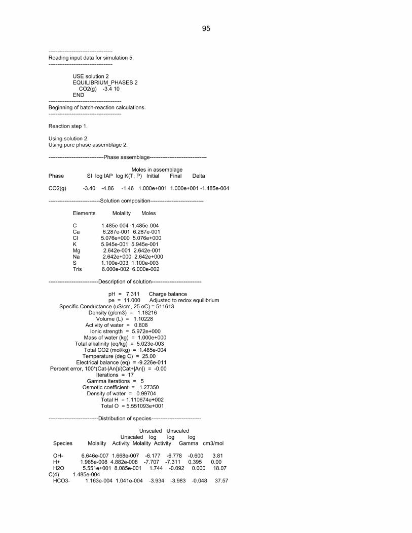
95

------------------------------------ Reading input data for simulation 5. ------------------------------------ USE solution 2 EQUILIBRIUM_PHASES 2 CO2(g) -3.4 10 END ----------------------------------------- Beginning of batch-reaction calculations. ----------------------------------------- Reaction step 1. Using solution 2. Using pure phase assemblage 2. -------------------------------Phase assemblage-------------------------------- Moles in assemblage Phase SI log IAP log K(T, P) Initial Final Delta CO2(g) -3.40 -4.86 -1.46 1.000e+001 1.000e+001 -1.485e-004 -----------------------------Solution composition------------------------------ Elements Molality Moles C 1.485e-004 1.485e-004 Ca 6.287e-001 6.287e-001 Cl 5.076e+000 5.076e+000 K 5.945e-001 5.945e-001 Mg 2.642e-001 2.642e-001 Na 2.642e+000 2.642e+000 S 1.100e-003 1.100e-003 Tris 6.000e-002 6.000e-002 ----------------------------Description of solution---------------------------- pH = 7.311 Charge balance pe = 11.000 Adjusted to redox equilibrium Specific Conductance (uS/cm, 25 oC) = 511613 Density (g/cm3) = 1.18216 Volume (L) = 1.10228 Activity of water = 0.808 Ionic strength = 5.972e+000 Mass of water (kg) = 1.000e+000 Total alkalinity (eq/kg) = 5.023e-003 Total CO2 (mol/kg) = 1.485e-004 Temperature (deg C) = 25.00 Electrical balance (eq) = -9.226e-011 Percent error, 100*(Cat-|An|)/(Cat+|An|) = -0.00 Iterations = 17 Gamma iterations = 5 Osmotic coefficient = 1.27350 Density of water = 0.99704 Total H = 1.110674e+002 Total O = 5.551093e+001 ----------------------------Distribution of species---------------------------- Unscaled Unscaled Unscaled log log log Species Molality Activity Molality Activity Gamma cm3/mol OH- 6.646e-007 1.668e-007 -6.177 -6.778 -0.600 3.81 H+ 1.965e-008 4.882e-008 -7.707 -7.311 0.395 0.00 H2O 5.551e+001 8.085e-001 1.744 -0.092 0.000 18.07 C(4) 1.485e-004 HCO3- 1.163e-004 1.041e-004 -3.934 -3.983 -0.048 37.57

96

MgCO3 1.638e-005 1.638e-005 -4.786 -4.786 0.000 -17.09 CO3-2 9.484e-006 9.761e-008 -5.023 -7.010 -1.987 8.69 CO2 6.287e-006 1.380e-005 -5.202 -4.860 0.341 30.26 Ca 6.287e-001 Ca+2 6.287e-001 3.113e-001 -0.202 -0.507 -0.305 -14.29 Cl 5.076e+000 Cl- 5.076e+000 5.848e+000 0.705 0.767 0.062 20.09 K 5.945e-001 K+ 5.945e-001 2.470e-001 -0.226 -0.607 -0.381 12.11 Mg 2.642e-001 Mg+2 2.642e-001 1.980e-001 -0.578 -0.703 -0.125 -17.79 MgCO3 1.638e-005 1.638e-005 -4.786 -4.786 0.000 -17.09 MgOH+ 1.376e-005 5.091e-006 -4.861 -5.293 -0.432 (0) Na 2.642e+000 Na+ 2.642e+000 2.016e+000 0.422 0.304 -0.118 1.41 S(6) 1.100e-003 SO4-2 1.100e-003 2.413e-005 -2.959 -4.618 -1.659 26.83 HSO4- 1.272e-010 1.122e-010 -9.895 -9.950 -0.054 42.04 Tris 6.000e-002 (Tris)H+ 5.516e-002 2.351e-002 -1.258 -1.629 -0.370 (0) Tris 4.841e-003 4.098e-003 -2.315 -2.387 -0.072 (0) ------------------------------Saturation indices------------------------------- Phase SI log IAP log K(298 K, 1 atm) Anhydrite -0.90 -5.12 -4.22 CaSO4 Aragonite 0.70 -7.52 -8.22 CaCO3 Arcanite -4.06 -5.83 -1.78 K2SO4 Bischofite -4.18 0.28 4.46 MgCl2:6H2O Bloedite -7.35 -9.70 -2.35 Na2Mg(SO4)2:4H2O Brucite -3.38 -14.26 -10.88 Mg(OH)2 Burkeite -13.65 -14.42 -0.77 Na6CO3(SO4)2 Calcite 0.89 -7.52 -8.41 CaCO3 Carnallite -3.89 0.44 4.33 KMgCl3:6H2O CO2(g) -3.40 -4.86 -1.46 CO2 Pressure 0.0 atm, phi 1.000 Dolomite 1.85 -15.23 -17.08 CaMg(CO3)2 Epsomite -4.09 -5.97 -1.88 MgSO4:7H2O Gaylussite -4.96 -14.38 -9.42 CaNa2(CO3)2:5H2O Glaserite -6.95 -10.75 -3.80 NaK3(SO4)2 Glauberite -3.89 -9.13 -5.25 Na2Ca(SO4)2 Gypsum -0.73 -5.31 -4.58 CaSO4:2H2O H2O(g) -1.60 -0.09 1.50 H2O Halite -0.50 1.07 1.57 NaCl Hexahydrite -4.24 -5.87 -1.63 MgSO4:6H2O Kainite -5.25 -5.44 -0.19 KMgClSO4:3H2O Kalicinite -4.87 -14.93 -10.06 KHCO3 Kieserite -5.29 -5.41 -0.12 MgSO4:H2O Labile_S -7.65 -13.33 -5.67 Na4Ca(SO4)3:2H2O Leonhardite -4.80 -5.69 -0.89 MgSO4:4H2O Leonite -7.54 -11.52 -3.98 K2Mg(SO4)2:4H2O Magnesite 0.12 -7.71 -7.83 MgCO3 Mirabilite -3.72 -4.93 -1.21 Na2SO4:10H2O Misenite -70.24 -81.05 -10.81 K8H6(SO4)7 Nahcolite -3.28 -14.02 -10.74 NaHCO3 Natron -6.50 -7.32 -0.82 Na2CO3:10H2O Nesquehonite -2.82 -7.99 -5.17 MgCO3:3H2O Pentahydrite -4.50 -5.78 -1.28 MgSO4:5H2O Pirssonite -4.87 -14.10 -9.23 Na2Ca(CO3)2:2H2O Polyhalite -7.84 -21.59 -13.74 K2MgCa2(SO4)4:2H2O Portlandite -8.87 -14.06 -5.19 Ca(OH)2 Schoenite -7.38 -11.71 -4.33 K2Mg(SO4)2:6H2O Sylvite -0.74 0.16 0.90 KCl Syngenite -3.60 -11.05 -7.45 K2Ca(SO4)2:H2O Trona -9.22 -20.60 -11.38 Na3H(CO3)2:2H2O ------------------ End of simulation. ------------------

97

------------------------------------ Reading input data for simulation 6. ------------------------------------ USE solution 3 EQUILIBRIUM_PHASES 3 CO2(g) -3.4 10 END ----------------------------------------- Beginning of batch-reaction calculations. ----------------------------------------- Reaction step 1. Using solution 3. Using pure phase assemblage 3. -------------------------------Phase assemblage-------------------------------- Moles in assemblage Phase SI log IAP log K(T, P) Initial Final Delta CO2(g) -3.40 -4.86 -1.46 1.000e+001 1.000e+001 -2.715e-004 -----------------------------Solution composition------------------------------ Elements Molality Moles C 2.715e-004 2.715e-004 Ca 6.287e-001 6.287e-001 Cl 5.073e+000 5.073e+000 K 5.945e-001 5.945e-001 Mg 2.642e-001 2.642e-001 Na 2.642e+000 2.642e+000 S 1.100e-003 1.100e-003 Tris 6.000e-002 6.000e-002 ----------------------------Description of solution---------------------------- pH = 7.533 Charge balance pe = 11.000 Adjusted to redox equilibrium Specific Conductance (uS/cm, 25 oC) = 511233 Density (g/cm3) = 1.18214 Volume (L) = 1.10222 Activity of water = 0.809 Ionic strength = 5.969e+000 Mass of water (kg) = 1.000e+000 Total alkalinity (eq/kg) = 8.011e-003 Total CO2 (mol/kg) = 2.715e-004 Temperature (deg C) = 25.00 Electrical balance (eq) = -2.200e-010 Percent error, 100*(Cat-|An|)/(Cat+|An|) = -0.00 Iterations = 17 Gamma iterations = 5 Osmotic coefficient = 1.27329 Density of water = 0.99704 Total H = 1.110645e+002 Total O = 5.551118e+001 ----------------------------Distribution of species---------------------------- Unscaled Unscaled Unscaled log log log Species Molality Activity Molality Activity Gamma cm3/mol OH- 1.106e-006 2.779e-007 -5.956 -6.556 -0.600 3.81 H+ 1.181e-008 2.932e-008 -7.928 -7.533 0.395 0.00 H2O 5.551e+001 8.086e-001 1.744 -0.092 0.000 18.07

98

C(4) 2.715e-004 HCO3- 1.936e-004 1.733e-004 -3.713 -3.761 -0.048 37.57 MgCO3 4.534e-005 4.534e-005 -4.344 -4.344 0.000 -17.09 CO3-2 2.627e-005 2.707e-007 -4.580 -6.568 -1.987 8.68 CO2 6.287e-006 1.380e-005 -5.202 -4.860 0.341 30.26 Ca 6.287e-001 Ca+2 6.287e-001 3.106e-001 -0.202 -0.508 -0.306 -14.29 Cl 5.073e+000 Cl- 5.073e+000 5.844e+000 0.705 0.767 0.062 20.09 K 5.945e-001 K+ 5.945e-001 2.470e-001 -0.226 -0.607 -0.381 12.11 Mg 2.642e-001 Mg+2 2.642e-001 1.977e-001 -0.578 -0.704 -0.126 -17.79 MgCO3 4.534e-005 4.534e-005 -4.344 -4.344 0.000 -17.09 MgOH+ 2.287e-005 8.462e-006 -4.641 -5.073 -0.432 (0) Na 2.642e+000 Na+ 2.642e+000 2.015e+000 0.422 0.304 -0.118 1.41 S(6) 1.100e-003 SO4-2 1.100e-003 2.413e-005 -2.959 -4.617 -1.659 26.83 HSO4- 7.638e-011 6.741e-011 -10.117 -10.171 -0.054 42.04 Tris 6.000e-002 (Tris)H+ 5.235e-002 2.231e-002 -1.281 -1.652 -0.370 (0) Tris 7.650e-003 6.476e-003 -2.116 -2.189 -0.072 (0) ------------------------------Saturation indices------------------------------- Phase SI log IAP log K(298 K, 1 atm) Anhydrite -0.90 -5.13 -4.22 CaSO4 Aragonite 1.14 -7.08 -8.22 CaCO3 Arcanite -4.06 -5.83 -1.78 K2SO4 Bischofite -4.18 0.28 4.46 MgCl2:6H2O Bloedite -7.35 -9.70 -2.35 Na2Mg(SO4)2:4H2O Brucite -2.94 -13.82 -10.88 Mg(OH)2 Burkeite -13.20 -13.98 -0.77 Na6CO3(SO4)2 Calcite 1.33 -7.08 -8.41 CaCO3 Carnallite -3.89 0.44 4.33 KMgCl3:6H2O CO2(g) -3.40 -4.86 -1.46 CO2 Pressure 0.0 atm, phi 1.000 Dolomite 2.74 -14.35 -17.08 CaMg(CO3)2 Epsomite -4.09 -5.97 -1.88 MgSO4:7H2O Gaylussite -4.07 -13.50 -9.42 CaNa2(CO3)2:5H2O Glaserite -6.95 -10.75 -3.80 NaK3(SO4)2 Glauberite -3.89 -9.13 -5.25 Na2Ca(SO4)2 Gypsum -0.73 -5.31 -4.58 CaSO4:2H2O H2O(g) -1.60 -0.09 1.50 H2O Halite -0.50 1.07 1.57 NaCl Hexahydrite -4.24 -5.88 -1.63 MgSO4:6H2O Kainite -5.25 -5.44 -0.19 KMgClSO4:3H2O Kalicinite -4.65 -14.71 -10.06 KHCO3 Kieserite -5.29 -5.41 -0.12 MgSO4:H2O Labile_S -7.66 -13.33 -5.67 Na4Ca(SO4)3:2H2O Leonhardite -4.80 -5.69 -0.89 MgSO4:4H2O Leonite -7.54 -11.52 -3.98 K2Mg(SO4)2:4H2O Magnesite 0.56 -7.27 -7.83 MgCO3 Mirabilite -3.72 -4.93 -1.21 Na2SO4:10H2O Misenite -71.57 -82.38 -10.81 K8H6(SO4)7 Nahcolite -3.05 -13.80 -10.74 NaHCO3 Natron -6.06 -6.88 -0.82 Na2CO3:10H2O Nesquehonite -2.38 -7.55 -5.17 MgCO3:3H2O Pentahydrite -4.50 -5.78 -1.28 MgSO4:5H2O Pirssonite -3.98 -13.22 -9.23 Na2Ca(CO3)2:2H2O Polyhalite -7.84 -21.59 -13.74 K2MgCa2(SO4)4:2H2O Portlandite -8.43 -13.62 -5.19 Ca(OH)2 Schoenite -7.38 -11.71 -4.33 K2Mg(SO4)2:6H2O Sylvite -0.74 0.16 0.90 KCl Syngenite -3.60 -11.05 -7.45 K2Ca(SO4)2:H2O Trona -8.56 -19.94 -11.38 Na3H(CO3)2:2H2O ------------------

99

End of simulation. ------------------ ------------------------------------ Reading input data for simulation 7. ------------------------------------ USE solution 4 EQUILIBRIUM_PHASES 4 CO2(g) -3.4 10 END ----------------------------------------- Beginning of batch-reaction calculations. ----------------------------------------- Reaction step 1. Using solution 4. Using pure phase assemblage 4. -------------------------------Phase assemblage-------------------------------- Moles in assemblage Phase SI log IAP log K(T, P) Initial Final Delta CO2(g) -3.40 -4.86 -1.46 1.000e+001 1.000e+001 -4.329e-004 -----------------------------Solution composition------------------------------ Elements Molality Moles C 4.329e-004 4.329e-004 Ca 6.287e-001 6.287e-001 Cl 5.070e+000 5.070e+000 K 5.945e-001 5.945e-001 Mg 2.642e-001 2.642e-001 Na 2.642e+000 2.642e+000 S 1.100e-003 1.100e-003 Tris 6.010e-002 6.010e-002 ----------------------------Description of solution---------------------------- pH = 7.691 Charge balance pe = 11.000 Adjusted to redox equilibrium Specific Conductance (uS/cm, 25 oC) = 510860 Density (g/cm3) = 1.18213 Volume (L) = 1.10216 Activity of water = 0.809 Ionic strength = 5.966e+000 Mass of water (kg) = 1.000e+000 Total alkalinity (eq/kg) = 1.105e-002 Total CO2 (mol/kg) = 4.329e-004 Temperature (deg C) = 25.00 Electrical balance (eq) = -3.834e-010 Percent error, 100*(Cat-|An|)/(Cat+|An|) = -0.00 Iterations = 18 Gamma iterations = 5 Osmotic coefficient = 1.27308 Density of water = 0.99704 Total H = 1.110616e+002 Total O = 5.551152e+001 ----------------------------Distribution of species---------------------------- Unscaled Unscaled Unscaled log log log Species Molality Activity Molality Activity Gamma cm3/mol OH- 1.591e-006 3.998e-007 -5.798 -6.398 -0.600 3.80 H+ 8.212e-009 2.038e-008 -8.086 -7.691 0.395 0.00

100

H2O 5.551e+001 8.086e-001 1.744 -0.092 0.000 18.07 C(4) 4.329e-004 HCO3- 2.786e-004 2.494e-004 -3.555 -3.603 -0.048 37.56 MgCO3 9.370e-005 9.370e-005 -4.028 -4.028 0.000 -17.09 CO3-2 5.434e-005 5.605e-007 -4.265 -6.251 -1.987 8.68 CO2 6.286e-006 1.380e-005 -5.202 -4.860 0.341 30.26 Ca 6.287e-001 Ca+2 6.287e-001 3.099e-001 -0.202 -0.509 -0.307 -14.29 Cl 5.070e+000 Cl- 5.070e+000 5.841e+000 0.705 0.766 0.061 20.09 K 5.945e-001 K+ 5.945e-001 2.470e-001 -0.226 -0.607 -0.381 12.11 Mg 2.642e-001 Mg+2 2.641e-001 1.973e-001 -0.578 -0.705 -0.127 -17.79 MgCO3 9.370e-005 9.370e-005 -4.028 -4.028 0.000 -17.09 MgOH+ 3.283e-005 1.215e-005 -4.484 -4.915 -0.432 (0) Na 2.642e+000 Na+ 2.642e+000 2.015e+000 0.422 0.304 -0.118 1.41 S(6) 1.100e-003 SO4-2 1.100e-003 2.414e-005 -2.959 -4.617 -1.659 26.83 HSO4- 5.308e-011 4.686e-011 -10.275 -10.329 -0.054 42.04 Tris 6.010e-002 (Tris)H+ 4.966e-002 2.116e-002 -1.304 -1.674 -0.370 (0) Tris 1.044e-002 8.839e-003 -1.981 -2.054 -0.072 (0) ------------------------------Saturation indices------------------------------- Phase SI log IAP log K(298 K, 1 atm) Anhydrite -0.90 -5.13 -4.22 CaSO4 Aragonite 1.46 -6.76 -8.22 CaCO3 Arcanite -4.06 -5.83 -1.78 K2SO4 Bischofite -4.18 0.27 4.46 MgCl2:6H2O Bloedite -7.35 -9.70 -2.35 Na2Mg(SO4)2:4H2O Brucite -2.62 -13.50 -10.88 Mg(OH)2 Burkeite -12.89 -13.66 -0.77 Na6CO3(SO4)2 Calcite 1.65 -6.76 -8.41 CaCO3 Carnallite -3.90 0.43 4.33 KMgCl3:6H2O CO2(g) -3.40 -4.86 -1.46 CO2 Pressure 0.0 atm, phi 1.000 Dolomite 3.37 -13.72 -17.08 CaMg(CO3)2 Epsomite -4.09 -5.97 -1.88 MgSO4:7H2O Gaylussite -3.44 -12.86 -9.42 CaNa2(CO3)2:5H2O Glaserite -6.95 -10.75 -3.80 NaK3(SO4)2 Glauberite -3.89 -9.13 -5.25 Na2Ca(SO4)2 Gypsum -0.73 -5.31 -4.58 CaSO4:2H2O H2O(g) -1.60 -0.09 1.50 H2O Halite -0.50 1.07 1.57 NaCl Hexahydrite -4.24 -5.88 -1.63 MgSO4:6H2O Kainite -5.25 -5.44 -0.19 KMgClSO4:3H2O Kalicinite -4.49 -14.55 -10.06 KHCO3 Kieserite -5.29 -5.41 -0.12 MgSO4:H2O Labile_S -7.66 -13.33 -5.67 Na4Ca(SO4)3:2H2O Leonhardite -4.80 -5.69 -0.89 MgSO4:4H2O Leonite -7.54 -11.52 -3.98 K2Mg(SO4)2:4H2O Magnesite 0.88 -6.96 -7.83 MgCO3 Mirabilite -3.72 -4.93 -1.21 Na2SO4:10H2O Misenite -72.52 -83.32 -10.81 K8H6(SO4)7 Nahcolite -2.90 -13.64 -10.74 NaHCO3 Natron -5.74 -6.57 -0.82 Na2CO3:10H2O Nesquehonite -2.07 -7.23 -5.17 MgCO3:3H2O Pentahydrite -4.50 -5.78 -1.28 MgSO4:5H2O Pirssonite -3.35 -12.59 -9.23 Na2Ca(CO3)2:2H2O Polyhalite -7.85 -21.59 -13.74 K2MgCa2(SO4)4:2H2O Portlandite -8.12 -13.31 -5.19 Ca(OH)2 Schoenite -7.38 -11.71 -4.33 K2Mg(SO4)2:6H2O Sylvite -0.74 0.16 0.90 KCl Syngenite -3.60 -11.05 -7.45 K2Ca(SO4)2:H2O Trona -8.08 -19.47 -11.38 Na3H(CO3)2:2H2O

101

------------------ End of simulation. ------------------ ------------------------------------ Reading input data for simulation 8. ------------------------------------ USE solution 5 EQUILIBRIUM_PHASES 5 CO2(g) -3.4 10 END ----------------------------------------- Beginning of batch-reaction calculations. ----------------------------------------- Reaction step 1. Using solution 5. Using pure phase assemblage 5. -------------------------------Phase assemblage-------------------------------- Moles in assemblage Phase SI log IAP log K(T, P) Initial Final Delta CO2(g) -3.40 -4.86 -1.46 1.000e+001 9.999e+000 -7.130e-004 -----------------------------Solution composition------------------------------ Elements Molality Moles C 7.130e-004 7.130e-004 Ca 6.287e-001 6.287e-001 Cl 5.066e+000 5.066e+000 K 5.945e-001 5.945e-001 Mg 2.642e-001 2.642e-001 Na 2.642e+000 2.642e+000 S 1.100e-003 1.100e-003 Tris 6.000e-002 6.000e-002 ----------------------------Description of solution---------------------------- pH = 7.849 Charge balance pe = 11.000 Adjusted to redox equilibrium Specific Conductance (uS/cm, 25 oC) = 510349 Density (g/cm3) = 1.18209 Volume (L) = 1.10208 Activity of water = 0.809 Ionic strength = 5.962e+000 Mass of water (kg) = 1.000e+000 Total alkalinity (eq/kg) = 1.500e-002 Total CO2 (mol/kg) = 7.130e-004 Temperature (deg C) = 25.00 Electrical balance (eq) = -5.752e-010 Percent error, 100*(Cat-|An|)/(Cat+|An|) = -0.00 Iterations = 18 Gamma iterations = 5 Osmotic coefficient = 1.27279 Density of water = 0.99704 Total H = 1.110575e+002 Total O = 5.551210e+001 ----------------------------Distribution of species---------------------------- Unscaled Unscaled Unscaled log log log Species Molality Activity Molality Activity Gamma cm3/mol OH- 2.288e-006 5.755e-007 -5.641 -6.240 -0.599 3.80

102

H+ 5.713e-009 1.416e-008 -8.243 -7.849 0.394 0.00 H2O 5.551e+001 8.088e-001 1.744 -0.092 0.000 18.07 C(4) 7.130e-004 HCO3- 4.008e-004 3.590e-004 -3.397 -3.445 -0.048 37.55 MgCO3 1.935e-004 1.935e-004 -3.713 -3.713 0.000 -17.09 CO3-2 1.124e-004 1.161e-006 -3.949 -5.935 -1.986 8.67 CO2 6.286e-006 1.380e-005 -5.202 -4.860 0.341 30.26 Ca 6.287e-001 Ca+2 6.287e-001 3.089e-001 -0.202 -0.510 -0.309 -14.29 Cl 5.066e+000 Cl- 5.066e+000 5.836e+000 0.705 0.766 0.061 20.09 K 5.945e-001 K+ 5.945e-001 2.471e-001 -0.226 -0.607 -0.381 12.11 Mg 2.642e-001 Mg+2 2.640e-001 1.967e-001 -0.578 -0.706 -0.128 -17.79 MgCO3 1.935e-004 1.935e-004 -3.713 -3.713 0.000 -17.09 MgOH+ 4.708e-005 1.744e-005 -4.327 -4.758 -0.431 (0) Na 2.642e+000 Na+ 2.642e+000 2.014e+000 0.422 0.304 -0.118 1.41 S(6) 1.100e-003 SO4-2 1.100e-003 2.415e-005 -2.959 -4.617 -1.659 26.82 HSO4- 3.688e-011 3.257e-011 -10.433 -10.487 -0.054 42.04 Tris 6.000e-002 (Tris)H+ 4.607e-002 1.963e-002 -1.337 -1.707 -0.371 (0) Tris 1.394e-002 1.180e-002 -1.856 -1.928 -0.072 (0) ------------------------------Saturation indices------------------------------- Phase SI log IAP log K(298 K, 1 atm) Anhydrite -0.90 -5.13 -4.22 CaSO4 Aragonite 1.77 -6.45 -8.22 CaCO3 Arcanite -4.06 -5.83 -1.78 K2SO4 Bischofite -4.18 0.27 4.46 MgCl2:6H2O Bloedite -7.35 -9.70 -2.35 Na2Mg(SO4)2:4H2O Brucite -2.31 -13.19 -10.88 Mg(OH)2 Burkeite -12.57 -13.34 -0.77 Na6CO3(SO4)2 Calcite 1.96 -6.45 -8.41 CaCO3 Carnallite -3.90 0.43 4.33 KMgCl3:6H2O CO2(g) -3.40 -4.86 -1.46 CO2 Pressure 0.0 atm, phi 1.000 Dolomite 4.00 -13.09 -17.08 CaMg(CO3)2 Epsomite -4.09 -5.97 -1.88 MgSO4:7H2O Gaylussite -2.81 -12.23 -9.42 CaNa2(CO3)2:5H2O Glaserite -6.95 -10.75 -3.80 NaK3(SO4)2 Glauberite -3.89 -9.14 -5.25 Na2Ca(SO4)2 Gypsum -0.73 -5.31 -4.58 CaSO4:2H2O H2O(g) -1.60 -0.09 1.50 H2O Halite -0.50 1.07 1.57 NaCl Hexahydrite -4.24 -5.88 -1.63 MgSO4:6H2O Kainite -5.25 -5.44 -0.19 KMgClSO4:3H2O Kalicinite -4.33 -14.39 -10.06 KHCO3 Kieserite -5.29 -5.42 -0.12 MgSO4:H2O Labile_S -7.66 -13.33 -5.67 Na4Ca(SO4)3:2H2O Leonhardite -4.81 -5.69 -0.89 MgSO4:4H2O Leonite -7.54 -11.52 -3.98 K2Mg(SO4)2:4H2O Magnesite 1.19 -6.64 -7.83 MgCO3 Mirabilite -3.72 -4.93 -1.21 Na2SO4:10H2O Misenite -73.46 -84.27 -10.81 K8H6(SO4)7 Nahcolite -2.74 -13.48 -10.74 NaHCO3 Natron -5.42 -6.25 -0.82 Na2CO3:10H2O Nesquehonite -1.75 -6.92 -5.17 MgCO3:3H2O Pentahydrite -4.50 -5.78 -1.28 MgSO4:5H2O Pirssonite -2.72 -11.96 -9.23 Na2Ca(CO3)2:2H2O Polyhalite -7.85 -21.59 -13.74 K2MgCa2(SO4)4:2H2O Portlandite -7.80 -12.99 -5.19 Ca(OH)2 Schoenite -7.38 -11.71 -4.33 K2Mg(SO4)2:6H2O Sylvite -0.74 0.16 0.90 KCl Syngenite -3.60 -11.05 -7.45 K2Ca(SO4)2:H2O Trona -7.61 -18.99 -11.38 Na3H(CO3)2:2H2O

103

------------------ End of simulation. ------------------ ------------------------------------ Reading input data for simulation 9. ------------------------------------ USE solution 6 EQUILIBRIUM_PHASES 6 CO2(g) -3.4 10 END ----------------------------------------- Beginning of batch-reaction calculations. ----------------------------------------- Reaction step 1. Using solution 6. Using pure phase assemblage 6. -------------------------------Phase assemblage-------------------------------- Moles in assemblage Phase SI log IAP log K(T, P) Initial Final Delta CO2(g) -3.40 -4.86 -1.46 1.000e+001 9.999e+000 -1.447e-003 -----------------------------Solution composition------------------------------ Elements Molality Moles C 1.447e-003 1.447e-003 Ca 6.287e-001 6.287e-001 Cl 5.059e+000 5.059e+000 K 5.945e-001 5.945e-001 Mg 2.642e-001 2.642e-001 Na 2.642e+000 2.642e+000 S 1.100e-003 1.100e-003 Tris 6.000e-002 6.000e-002 ----------------------------Description of solution---------------------------- pH = 8.057 Charge balance pe = 11.000 Adjusted to redox equilibrium Specific Conductance (uS/cm, 25 oC) = 509468 Density (g/cm3) = 1.18206 Volume (L) = 1.10195 Activity of water = 0.809 Ionic strength = 5.956e+000 Mass of water (kg) = 1.000e+000 Total alkalinity (eq/kg) = 2.200e-002 Total CO2 (mol/kg) = 1.447e-003 Temperature (deg C) = 25.00 Electrical balance (eq) = -3.454e-010 Percent error, 100*(Cat-|An|)/(Cat+|An|) = -0.00 Iterations = 19 Gamma iterations = 5 Osmotic coefficient = 1.27224 Density of water = 0.99704 Total H = 1.110506e+002 Total O = 5.551361e+001 ----------------------------Distribution of species---------------------------- Unscaled Unscaled Unscaled log log log Species Molality Activity Molality Activity Gamma cm3/mol

104

OH- 3.691e-006 9.294e-007 -5.433 -6.032 -0.599 3.79 H+ 3.544e-009 8.769e-009 -8.450 -8.057 0.393 0.00 H2O 5.551e+001 8.089e-001 1.744 -0.092 0.000 18.07 C(4) 1.447e-003 HCO3- 6.469e-004 5.798e-004 -3.189 -3.237 -0.048 37.54 MgCO3 5.020e-004 5.020e-004 -3.299 -3.299 0.000 -17.09 CO3-2 2.924e-004 3.028e-006 -3.534 -5.519 -1.985 8.66 CO2 6.287e-006 1.380e-005 -5.202 -4.860 0.341 30.26 Ca 6.287e-001 Ca+2 6.287e-001 3.073e-001 -0.202 -0.512 -0.311 -14.29 Cl 5.059e+000 Cl- 5.059e+000 5.826e+000 0.704 0.765 0.061 20.09 K 5.945e-001 K+ 5.945e-001 2.471e-001 -0.226 -0.607 -0.381 12.11 Mg 2.642e-001 Mg+2 2.637e-001 1.956e-001 -0.579 -0.709 -0.130 -17.79 MgCO3 5.020e-004 5.020e-004 -3.299 -3.299 0.000 -17.09 MgOH+ 7.555e-005 2.802e-005 -4.122 -4.553 -0.431 (0) Na 2.642e+000 Na+ 2.642e+000 2.013e+000 0.422 0.304 -0.118 1.40 S(6) 1.100e-003 SO4-2 1.100e-003 2.416e-005 -2.959 -4.617 -1.658 26.81 HSO4- 2.284e-011 2.018e-011 -10.641 -10.695 -0.054 42.04 Tris 6.000e-002 (Tris)H+ 4.031e-002 1.717e-002 -1.395 -1.765 -0.371 (0) Tris 1.969e-002 1.667e-002 -1.706 -1.778 -0.072 (0) ------------------------------Saturation indices------------------------------- Phase SI log IAP log K(298 K, 1 atm) Anhydrite -0.90 -5.13 -4.22 CaSO4 Aragonite 2.19 -6.03 -8.22 CaCO3 Arcanite -4.05 -5.83 -1.78 K2SO4 Bischofite -4.19 0.27 4.46 MgCl2:6H2O Bloedite -7.36 -9.70 -2.35 Na2Mg(SO4)2:4H2O Brucite -1.89 -12.77 -10.88 Mg(OH)2 Burkeite -12.16 -12.93 -0.77 Na6CO3(SO4)2 Calcite 2.37 -6.03 -8.41 CaCO3 Carnallite -3.90 0.43 4.33 KMgCl3:6H2O CO2(g) -3.40 -4.86 -1.46 CO2 Pressure 0.0 atm, phi 1.000 Dolomite 4.82 -12.26 -17.08 CaMg(CO3)2 Epsomite -4.09 -5.97 -1.88 MgSO4:7H2O Gaylussite -1.98 -11.40 -9.42 CaNa2(CO3)2:5H2O Glaserite -6.95 -10.75 -3.80 NaK3(SO4)2 Glauberite -3.89 -9.14 -5.25 Na2Ca(SO4)2 Gypsum -0.73 -5.31 -4.58 CaSO4:2H2O H2O(g) -1.59 -0.09 1.50 H2O Halite -0.50 1.07 1.57 NaCl Hexahydrite -4.24 -5.88 -1.63 MgSO4:6H2O Kainite -5.25 -5.44 -0.19 KMgClSO4:3H2O Kalicinite -4.12 -14.18 -10.06 KHCO3 Kieserite -5.29 -5.42 -0.12 MgSO4:H2O Labile_S -7.66 -13.33 -5.67 Na4Ca(SO4)3:2H2O Leonhardite -4.81 -5.69 -0.89 MgSO4:4H2O Leonite -7.55 -11.52 -3.98 K2Mg(SO4)2:4H2O Magnesite 1.61 -6.23 -7.83 MgCO3 Mirabilite -3.72 -4.93 -1.21 Na2SO4:10H2O Misenite -74.71 -85.52 -10.81 K8H6(SO4)7 Nahcolite -2.53 -13.27 -10.74 NaHCO3 Natron -5.01 -5.83 -0.82 Na2CO3:10H2O Nesquehonite -1.34 -6.50 -5.17 MgCO3:3H2O Pentahydrite -4.50 -5.79 -1.28 MgSO4:5H2O Pirssonite -1.89 -11.13 -9.23 Na2Ca(CO3)2:2H2O Polyhalite -7.86 -21.60 -13.74 K2MgCa2(SO4)4:2H2O Portlandite -7.39 -12.58 -5.19 Ca(OH)2 Schoenite -7.38 -11.71 -4.33 K2Mg(SO4)2:6H2O Sylvite -0.74 0.16 0.90 KCl Syngenite -3.60 -11.05 -7.45 K2Ca(SO4)2:H2O Trona -6.98 -18.37 -11.38 Na3H(CO3)2:2H2O

105

------------------ End of simulation. ------------------ ------------------------------------- Reading input data for simulation 10. ------------------------------------- USE solution 7 EQUILIBRIUM_PHASES 7 CO2(g) -3.4 10 END ----------------------------------------- Beginning of batch-reaction calculations. ----------------------------------------- Reaction step 1. Using solution 7. Using pure phase assemblage 7. -------------------------------Phase assemblage-------------------------------- Moles in assemblage Phase SI log IAP log K(T, P) Initial Final Delta CO2(g) -3.40 -4.86 -1.46 1.000e+001 9.997e+000 -2.747e-003 -----------------------------Solution composition------------------------------ Elements Molality Moles C 2.747e-003 2.747e-003 Ca 6.287e-001 6.287e-001 Cl 5.051e+000 5.051e+000 K 5.946e-001 5.945e-001 Mg 2.643e-001 2.642e-001 Na 2.643e+000 2.642e+000 S 1.100e-003 1.100e-003 Tris 6.000e-002 6.000e-002 ----------------------------Description of solution---------------------------- pH = 8.232 Charge balance pe = 11.000 Adjusted to redox equilibrium Specific Conductance (uS/cm, 25 oC) = 508471 Density (g/cm3) = 1.18204 Volume (L) = 1.10182 Activity of water = 0.809 Ionic strength = 5.949e+000 Mass of water (kg) = 1.000e+000 Total alkalinity (eq/kg) = 2.997e-002 Total CO2 (mol/kg) = 2.747e-003 Temperature (deg C) = 25.00 Electrical balance (eq) = 2.213e-009 Percent error, 100*(Cat-|An|)/(Cat+|An|) = 0.00 Iterations = 20 Gamma iterations = 5 Osmotic coefficient = 1.27153 Density of water = 0.99704 Total H = 1.110428e+002 Total O = 5.551627e+001 ----------------------------Distribution of species---------------------------- Unscaled Unscaled Unscaled log log log Species Molality Activity Molality Activity Gamma cm3/mol

106

OH- 5.521e-006 1.392e-006 -5.258 -5.856 -0.598 3.78 H+ 2.372e-009 5.855e-009 -8.625 -8.232 0.393 0.00 H2O 5.551e+001 8.092e-001 1.744 -0.092 0.000 18.07 C(4) 2.747e-003 MgCO3 1.118e-003 1.118e-003 -2.952 -2.952 0.000 -17.09 HCO3- 9.685e-004 8.686e-004 -3.014 -3.061 -0.047 37.52 CO3-2 6.540e-004 6.792e-006 -3.184 -5.168 -1.984 8.65 CO2 6.288e-006 1.380e-005 -5.202 -4.860 0.341 30.26 Ca 6.287e-001 Ca+2 6.287e-001 3.056e-001 -0.202 -0.515 -0.313 -14.29 Cl 5.051e+000 Cl- 5.051e+000 5.815e+000 0.703 0.765 0.061 20.09 K 5.946e-001 K+ 5.946e-001 2.472e-001 -0.226 -0.607 -0.381 12.10 Mg 2.643e-001 Mg+2 2.630e-001 1.942e-001 -0.580 -0.712 -0.132 -17.80 MgCO3 1.118e-003 1.118e-003 -2.952 -2.952 0.000 -17.09 MgOH+ 1.122e-004 4.167e-005 -3.950 -4.380 -0.430 (0) Na 2.643e+000 Na+ 2.643e+000 2.012e+000 0.422 0.304 -0.118 1.40 S(6) 1.100e-003 SO4-2 1.100e-003 2.417e-005 -2.959 -4.617 -1.658 26.81 HSO4- 1.525e-011 1.348e-011 -10.817 -10.870 -0.054 42.04 Tris 6.000e-002 (Tris)H+ 3.466e-002 1.476e-002 -1.460 -1.831 -0.371 (0) Tris 2.534e-002 2.146e-002 -1.596 -1.668 -0.072 (0) ------------------------------Saturation indices------------------------------- Phase SI log IAP log K(298 K, 1 atm) Anhydrite -0.91 -5.13 -4.22 CaSO4 Aragonite 2.54 -5.68 -8.22 CaCO3 Arcanite -4.05 -5.83 -1.78 K2SO4 Bischofite -4.19 0.27 4.46 MgCl2:6H2O Bloedite -7.36 -9.71 -2.35 Na2Mg(SO4)2:4H2O Brucite -1.54 -12.42 -10.88 Mg(OH)2 Burkeite -11.81 -12.58 -0.77 Na6CO3(SO4)2 Calcite 2.72 -5.68 -8.41 CaCO3 Carnallite -3.91 0.42 4.33 KMgCl3:6H2O CO2(g) -3.40 -4.86 -1.46 CO2 Pressure 0.0 atm, phi 1.000 Dolomite 5.52 -11.56 -17.08 CaMg(CO3)2 Epsomite -4.09 -5.97 -1.88 MgSO4:7H2O Gaylussite -1.28 -10.70 -9.42 CaNa2(CO3)2:5H2O Glaserite -6.95 -10.75 -3.80 NaK3(SO4)2 Glauberite -3.90 -9.14 -5.25 Na2Ca(SO4)2 Gypsum -0.73 -5.32 -4.58 CaSO4:2H2O H2O(g) -1.59 -0.09 1.50 H2O Halite -0.50 1.07 1.57 NaCl Hexahydrite -4.25 -5.88 -1.63 MgSO4:6H2O Kainite -5.25 -5.45 -0.19 KMgClSO4:3H2O Kalicinite -3.95 -14.01 -10.06 KHCO3 Kieserite -5.30 -5.42 -0.12 MgSO4:H2O Labile_S -7.66 -13.33 -5.67 Na4Ca(SO4)3:2H2O Leonhardite -4.81 -5.70 -0.89 MgSO4:4H2O Leonite -7.55 -11.53 -3.98 K2Mg(SO4)2:4H2O Magnesite 1.95 -5.88 -7.83 MgCO3 Mirabilite -3.72 -4.93 -1.21 Na2SO4:10H2O Misenite -75.76 -86.57 -10.81 K8H6(SO4)7 Nahcolite -2.35 -13.10 -10.74 NaHCO3 Natron -4.66 -5.48 -0.82 Na2CO3:10H2O Nesquehonite -0.99 -6.16 -5.17 MgCO3:3H2O Pentahydrite -4.50 -5.79 -1.28 MgSO4:5H2O Pirssonite -1.19 -10.43 -9.23 Na2Ca(CO3)2:2H2O Polyhalite -7.86 -21.61 -13.74 K2MgCa2(SO4)4:2H2O Portlandite -7.04 -12.23 -5.19 Ca(OH)2 Schoenite -7.38 -11.71 -4.33 K2Mg(SO4)2:6H2O Sylvite -0.74 0.16 0.90 KCl Syngenite -3.61 -11.05 -7.45 K2Ca(SO4)2:H2O

107

Trona -6.46 -17.84 -11.38 Na3H(CO3)2:2H2O ------------------ End of simulation. ------------------ ------------------------------------- Reading input data for simulation 11. ------------------------------------- USE solution 8 EQUILIBRIUM_PHASES 8 CO2(g) -3.4 10 END ----------------------------------------- Beginning of batch-reaction calculations. ----------------------------------------- Reaction step 1. Using solution 8. Just 1.2x's LSPW (no Tris) Using pure phase assemblage 8. -------------------------------Phase assemblage-------------------------------- Moles in assemblage Phase SI log IAP log K(T, P) Initial Final Delta CO2(g) -3.40 -4.86 -1.46 1.000e+001 1.000e+001 -7.723e-006 -----------------------------Solution composition------------------------------ Elements Molality Moles C 7.723e-006 7.723e-006 Ca 6.287e-001 6.287e-001 Cl 5.020e+000 5.020e+000 K 5.945e-001 5.945e-001 Mg 2.642e-001 2.642e-001 Na 2.642e+000 2.642e+000 S 1.101e-003 1.101e-003 ----------------------------Description of solution---------------------------- pH = 5.404 Charge balance pe = 11.000 Adjusted to redox equilibrium Specific Conductance (uS/cm, 25 oC) = 505300 Density (g/cm3) = 1.17504 Volume (L) = 1.10105 Activity of water = 0.811 Ionic strength = 5.917e+000 Mass of water (kg) = 1.000e+000 Total alkalinity (eq/kg) = 1.696e-014 Total CO2 (mol/kg) = 7.723e-006 Temperature (deg C) = 25.00 Electrical balance (eq) = 1.808e-014 Percent error, 100*(Cat-|An|)/(Cat+|An|) = 0.00 Iterations = 15 Gamma iterations = 4 Osmotic coefficient = 1.27274 Density of water = 0.99704 Total H = 1.110124e+002 Total O = 5.551064e+001 ----------------------------Distribution of species---------------------------- Unscaled Unscaled Unscaled log log log Species Molality Activity Molality Activity Gamma cm3/mol

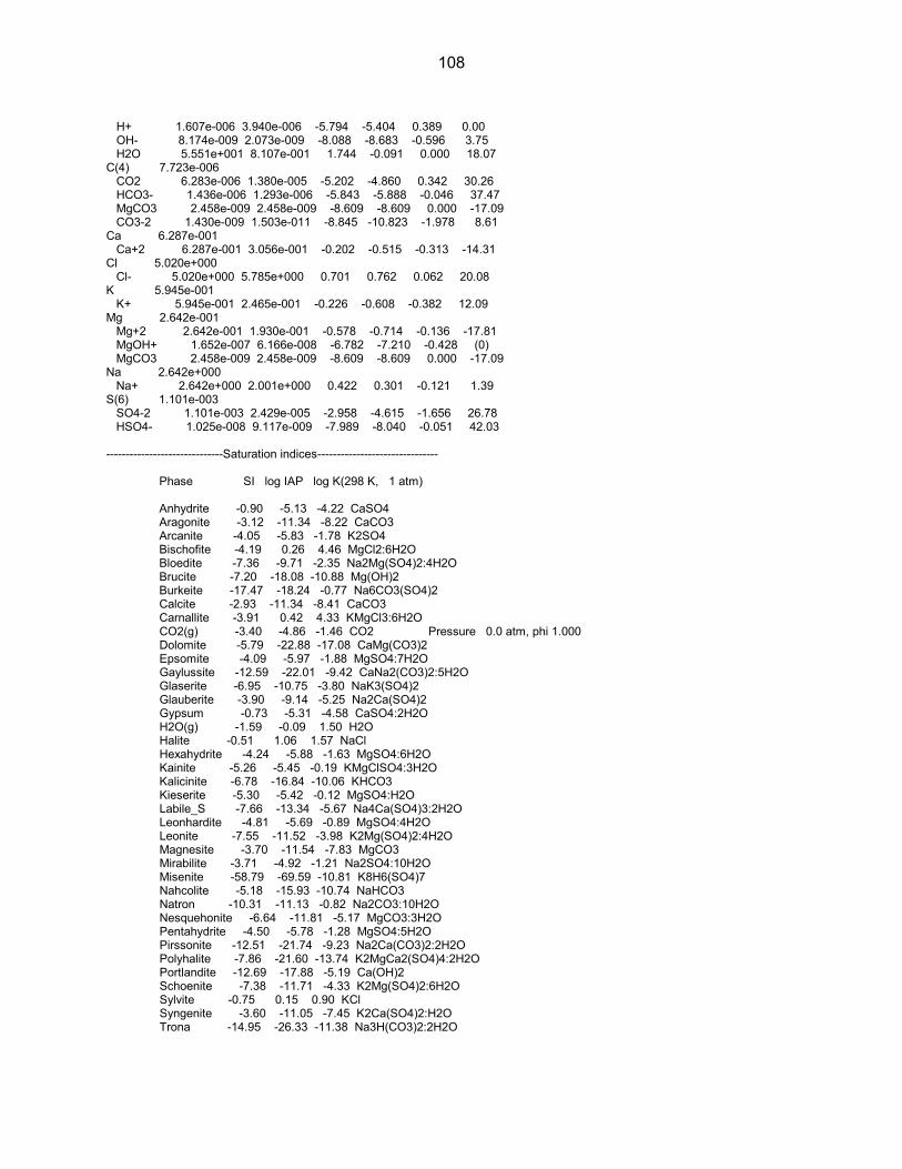
108

H+ 1.607e-006 3.940e-006 -5.794 -5.404 0.389 0.00 OH- 8.174e-009 2.073e-009 -8.088 -8.683 -0.596 3.75 H2O 5.551e+001 8.107e-001 1.744 -0.091 0.000 18.07 C(4) 7.723e-006 CO2 6.283e-006 1.380e-005 -5.202 -4.860 0.342 30.26 HCO3- 1.436e-006 1.293e-006 -5.843 -5.888 -0.046 37.47 MgCO3 2.458e-009 2.458e-009 -8.609 -8.609 0.000 -17.09 CO3-2 1.430e-009 1.503e-011 -8.845 -10.823 -1.978 8.61 Ca 6.287e-001 Ca+2 6.287e-001 3.056e-001 -0.202 -0.515 -0.313 -14.31 Cl 5.020e+000 Cl- 5.020e+000 5.785e+000 0.701 0.762 0.062 20.08 K 5.945e-001 K+ 5.945e-001 2.465e-001 -0.226 -0.608 -0.382 12.09 Mg 2.642e-001 Mg+2 2.642e-001 1.930e-001 -0.578 -0.714 -0.136 -17.81 MgOH+ 1.652e-007 6.166e-008 -6.782 -7.210 -0.428 (0) MgCO3 2.458e-009 2.458e-009 -8.609 -8.609 0.000 -17.09 Na 2.642e+000 Na+ 2.642e+000 2.001e+000 0.422 0.301 -0.121 1.39 S(6) 1.101e-003 SO4-2 1.101e-003 2.429e-005 -2.958 -4.615 -1.656 26.78 HSO4- 1.025e-008 9.117e-009 -7.989 -8.040 -0.051 42.03 ------------------------------Saturation indices------------------------------- Phase SI log IAP log K(298 K, 1 atm) Anhydrite -0.90 -5.13 -4.22 CaSO4 Aragonite -3.12 -11.34 -8.22 CaCO3 Arcanite -4.05 -5.83 -1.78 K2SO4 Bischofite -4.19 0.26 4.46 MgCl2:6H2O Bloedite -7.36 -9.71 -2.35 Na2Mg(SO4)2:4H2O Brucite -7.20 -18.08 -10.88 Mg(OH)2 Burkeite -17.47 -18.24 -0.77 Na6CO3(SO4)2 Calcite -2.93 -11.34 -8.41 CaCO3 Carnallite -3.91 0.42 4.33 KMgCl3:6H2O CO2(g) -3.40 -4.86 -1.46 CO2 Pressure 0.0 atm, phi 1.000 Dolomite -5.79 -22.88 -17.08 CaMg(CO3)2 Epsomite -4.09 -5.97 -1.88 MgSO4:7H2O Gaylussite -12.59 -22.01 -9.42 CaNa2(CO3)2:5H2O Glaserite -6.95 -10.75 -3.80 NaK3(SO4)2 Glauberite -3.90 -9.14 -5.25 Na2Ca(SO4)2 Gypsum -0.73 -5.31 -4.58 CaSO4:2H2O H2O(g) -1.59 -0.09 1.50 H2O Halite -0.51 1.06 1.57 NaCl Hexahydrite -4.24 -5.88 -1.63 MgSO4:6H2O Kainite -5.26 -5.45 -0.19 KMgClSO4:3H2O Kalicinite -6.78 -16.84 -10.06 KHCO3 Kieserite -5.30 -5.42 -0.12 MgSO4:H2O Labile_S -7.66 -13.34 -5.67 Na4Ca(SO4)3:2H2O Leonhardite -4.81 -5.69 -0.89 MgSO4:4H2O Leonite -7.55 -11.52 -3.98 K2Mg(SO4)2:4H2O Magnesite -3.70 -11.54 -7.83 MgCO3 Mirabilite -3.71 -4.92 -1.21 Na2SO4:10H2O Misenite -58.79 -69.59 -10.81 K8H6(SO4)7 Nahcolite -5.18 -15.93 -10.74 NaHCO3 Natron -10.31 -11.13 -0.82 Na2CO3:10H2O Nesquehonite -6.64 -11.81 -5.17 MgCO3:3H2O Pentahydrite -4.50 -5.78 -1.28 MgSO4:5H2O Pirssonite -12.51 -21.74 -9.23 Na2Ca(CO3)2:2H2O Polyhalite -7.86 -21.60 -13.74 K2MgCa2(SO4)4:2H2O Portlandite -12.69 -17.88 -5.19 Ca(OH)2 Schoenite -7.38 -11.71 -4.33 K2Mg(SO4)2:6H2O Sylvite -0.75 0.15 0.90 KCl Syngenite -3.60 -11.05 -7.45 K2Ca(SO4)2:H2O Trona -14.95 -26.33 -11.38 Na3H(CO3)2:2H2O

109

------------------ End of simulation. ------------------ ------------------------------------- Reading input data for simulation 12. ------------------------------------- ------------------------------- End of Run after 0.348 Seconds. ------------------------------- B.4 pH BUFFER SOLUTIONS

Table B.1: As-Made Buffer Solutions for pH and pK’a Measurements (Units are mol/kg water)

Details Solution pH mu Na K Ca Mg Cl SO4 Tris si_

halite si_

gypsum

NaCl solutions for molar absorptivity coefficient (ε) determinations no CO2 0.05 3.22 0.05 0.050 - - - 0.050 - - -4.35 -

log PCO2 = -3.4 0.05m 3.22 0.05 0.050 - - - 0.050 - - -4.35 -

no CO2 0.05m 11.11 0.12 0.101 - - - 0.050 - - -4.11 -

log PCO2 = -3.4 0.05m 9.61 0.11 0.101 - - - 0.050 - - -4.10 -

no CO2 1.0m 3.10 1.01 1.005 - - - 1.005 - - -1.93 -

log PCO2 = -3.4 1.0m 3.10 1.01 1.005 - - - 1.005 - - -1.93 -

no CO2 1.0m 10.87 1.07 1.050 - - - 1.000 - - -1.92 -

log PCO2 = -3.4 1.0m 9.38 1.06 1.050 - - - 1.000 - - -1.92 -

no CO2 5.0m 2.66 5.04 5.041 - - - 5.041 - - -0.28 -

log PCO2 = -3.4 5.0m 2.66 5.04 5.041 - - - 5.041 - - -0.28 -

no CO2 5.0m 10.69 5.07 5.046 - - - 4.996 - - -0.29 -

log PCO2 = -3.4 5.0m 9.19 5.06 5.047 - - - 4.997 - - -0.29 -

Buffer solutions containing only Tris/TrisHCl buffer (Just Tris) no CO2 1 7.10 0.05 - - - - 0.046 - 0.0500 - -

no CO2 2 7.29 0.04 - - - - 0.044 - 0.0500 - -

no CO2 3 7.43 0.04 - - - - 0.042 - 0.0500 - -

no CO2 4 7.43 0.04 - - - - 0.042 - 0.0500 - -

no CO2 5 7.65 0.04 - - - - 0.038 - 0.0500 - -

no CO2 6 7.86 0.03 - - - - 0.033 - 0.0500 - -

no CO2 7 8.04 0.03 - - - - 0.028 - 0.0500 - -

log PCO2 = -3.4 1 7.09 0.05 - - - - 0.046 - 0.0500 - -

log PCO2 = -3.4 2 7.28 0.04 - - - - 0.044 - 0.0500 - -

log PCO2 = -3.4 3 7.42 0.04 - - - - 0.042 - 0.0500 - -

log PCO2 = -3.4 4 7.42 0.04 - - - - 0.042 - 0.0500 - -

log PCO2 = -3.4 5 7.63 0.04 - - - - 0.038 - 0.0500 - -

log PCO2 = -3.4 6 7.84 0.03 - - - - 0.033 - 0.0500 - -

log PCO2 = -3.4 7 8.01 0.03 - - - - 0.028 - 0.0500 - -

NaCl buffer solutions for pH and pka measurements

0.1 m NaCl

no CO2 1 7.15 0.10 0.045 - - - 0.100 - 0.0600 -4.14 -

no CO2 2 7.49 0.10 0.050 - - - 0.100 - 0.0601 -4.09 -

no CO2 3 7.71 0.10 0.055 - - - 0.100 - 0.0599 -4.05 -

110



halite si_

gypsum

no CO2 4 7.95 0.10 0.062 - - - 0.100 - 0.0599 -4.00 -

no CO2 5 8.13 0.10 0.068 - - - 0.100 - 0.0600 -3.96 -

no CO2 6 8.33 0.10 0.075 - - - 0.100 - 0.0598 -3.91 -

no CO2 7 8.49 0.10 0.080 - - - 0.100 - 0.0599 -3.89 -

no CO2 8 8.89 0.10 0.090 - - - 0.100 - 0.0598 -3.83 -

log PCO2 = -3.4 1 7.13 0.10 0.045 - - - 0.100 - 0.0600 -4.14 -

log PCO2 = -3.4 2 7.47 0.10 0.050 - - - 0.100 - 0.0601 -4.09 -

log PCO2 = -3.4 3 7.70 0.10 0.055 - - - 0.100 - 0.0599 -4.05 -

log PCO2 = -3.4 4 7.93 0.10 0.062 - - - 0.100 - 0.0599 -4.00 -

log PCO2 = -3.4 5 8.10 0.10 0.068 - - - 0.100 - 0.0600 -3.96 -

log PCO2 = -3.4 6 8.29 0.10 0.075 - - - 0.100 - 0.0598 -3.92 -

log PCO2 = -3.4 7 8.42 0.10 0.080 - - - 0.100 - 0.0599 -3.89 -

log PCO2 = -3.4 8 8.69 0.10 0.090 - - - 0.100 - 0.0598 -3.84 -

1.0 m NaCl

no CO2 1 7.04 1.02 0.962 - - - 1.019 - 0.0600 -1.95 -

no CO2 2a 7.29 1.02 0.965 - - - 1.020 - 0.0599 -1.95 -

no CO2 2b 7.28 1.02 0.967 - - - 1.022 - 0.0600 -1.95 -

no CO2 3 7.51 1.03 0.975 - - - 1.027 - 0.0600 -1.94 -

no CO2 4 7.85 1.03 0.982 - - - 1.027 - 0.0600 -1.94 -

no CO2 5 8.02 1.03 0.988 - - - 1.028 - 0.0599 -1.93 -

no CO2 6 8.18 1.03 0.995 - - - 1.030 - 0.0599 -1.93 -

log PCO2 = -3.4 1 7.03 1.02 0.962 - - - 1.019 - 0.0600 -1.95 -

log PCO2 = -3.4 2a 7.27 1.02 0.965 - - - 1.020 - 0.0599 -1.95 -

log PCO2 = -3.4 2b 7.26 1.02 0.967 - - - 1.022 - 0.0600 -1.95 -

log PCO2 = -3.4 3 7.49 1.03 0.975 - - - 1.027 - 0.0600 -1.94 -

log PCO2 = -3.4 4 7.82 1.03 0.982 - - - 1.027 - 0.0600 -1.94 -

log PCO2 = -3.4 5 7.99 1.03 0.988 - - - 1.028 - 0.0599 -1.93 -

log PCO2 = -3.4 6 8.13 1.03 0.995 - - - 1.030 - 0.0599 -1.93 -

1.0 m NaCl

no CO2 1 6.86 0.99 0.936 - - - 0.994 - 0.0600 -1.97 -

no CO2 2 7.18 1.00 0.944 - - - 1.000 - 0.0600 -1.96 -

no CO2 3 7.44 1.00 0.947 - - - 1.000 - 0.0600 -1.96 -

no CO2 4 7.62 1.00 0.950 - - - 1.000 - 0.0600 -1.96 -

no CO2 5 7.84 1.00 0.955 - - - 1.000 - 0.0600 -1.96 -

no CO2 6 8.02 1.00 0.960 - - - 1.000 - 0.0600 -1.96 -

log PCO2 = -3.4 1 6.84 0.99 0.936 - - - 0.994 - 0.0600 -1.97 -

log PCO2 = -3.4 2 7.16 1.00 0.944 - - - 1.000 - 0.0600 -1.96 -

log PCO2 = -3.4 3 7.42 1.00 0.947 - - - 1.000 - 0.0600 -1.96 -

log PCO2 = -3.4 4 7.60 1.00 0.950 - - - 1.000 - 0.0600 -1.96 -

log PCO2 = -3.4 5 7.81 1.00 0.955 - - - 1.000 - 0.0600 -1.96 -

log PCO2 = -3.4 6 7.98 1.00 0.960 - - - 1.000 - 0.0600 -1.96 -

5.0 m NaCl

no CO2 1 6.87 5.00 4.942 - - - 5.000 - 0.0595 -0.30 -

no CO2 2 7.18 5.00 4.942 - - - 4.999 - 0.0600 -0.30 -

no CO2 3 7.41 5.00 4.944 - - - 4.999 - 0.0600 -0.30 -

111



halite si_

gypsum

no CO2 4 7.64 5.00 4.948 - - - 5.000 - 0.0600 -0.30 -

no CO2 5 7.98 5.00 4.953 - - - 4.998 - 0.0600 -0.30 -

no CO2 6 8.16 5.00 4.959 - - - 4.999 - 0.0600 -0.30 -

log PCO2 = -3.4 1 6.84 5.00 4.942 - - - 5.000 - 0.0595 -0.30 -

log PCO2 = -3.4 2 7.15 5.00 4.942 - - - 4.999 - 0.0600 -0.30 -

log PCO2 = -3.4 3 7.38 5.00 4.944 - - - 4.999 - 0.0600 -0.30 -

log PCO2 = -3.4 4 7.61 5.00 4.948 - - - 5.000 - 0.0600 -0.30 -

log PCO2 = -3.4 5 7.93 5.00 4.953 - - - 4.998 - 0.0600 -0.30 -

log PCO2 = -3.4 6 8.09 5.00 4.959 - - - 4.999 - 0.0600 -0.30 -

L-SPW series buffer solutions for pH and pka measurements

1.57x's L-SPW

no CO2 1 6.94 7.67 3.405 0.766 0.810 0.341 6.520 0.0011 0.052 -0.11 -0.50

no CO2 2 7.12 7.67 3.405 0.766 0.810 0.341 6.520 0.0011 0.053 -0.11 -0.50

no CO2 3 7.26 7.67 3.405 0.766 0.810 0.341 6.519 0.0011 0.053 -0.11 -0.50

no CO2 4 7.45 7.67 3.405 0.766 0.810 0.341 6.517 0.0011 0.053 -0.11 -0.50

no CO2 5 7.65 7.67 3.405 0.766 0.810 0.341 6.514 0.0011 0.053 -0.11 -0.50

no CO2 6 7.94 7.66 3.405 0.766 0.810 0.341 6.508 0.0011 0.053 -0.11 -0.51

no CO2 7 8.45 7.65 3.405 0.766 0.810 0.341 6.493 0.0011 0.053 -0.11 -0.51

log PCO2 = -3.4 1 6.92 7.67 3.405 0.766 0.810 0.341 6.520 0.0011 0.052 -0.11 -0.50

log PCO2 = -3.4 2 7.11 7.67 3.405 0.766 0.810 0.341 6.520 0.0011 0.053 -0.11 -0.50

log PCO2 = -3.4 3 7.24 7.67 3.405 0.766 0.810 0.341 6.519 0.0011 0.053 -0.11 -0.50

log PCO2 = -3.4 4 7.42 7.67 3.405 0.766 0.810 0.341 6.517 0.0011 0.053 -0.11 -0.50

log PCO2 = -3.4 5 7.62 7.67 3.405 0.766 0.810 0.341 6.514 0.0011 0.053 -0.11 -0.50

log PCO2 = -3.4 6 7.87 7.66 3.405 0.766 0.810 0.341 6.508 0.0011 0.053 -0.11 -0.51

log PCO2 = -3.4 7 8.22 7.65 3.405 0.766 0.810 0.341 6.493 0.0011 0.053 -0.11 -0.51

no CO2 HCl 1 2.74 6.51 2.908 0.654 0.691 0.291 5.524 0.0010 - -0.37 -0.69

1.45x's L-SPW

no CO2 unbuffered 5.70 7.03 3.143 0.707 0.746 0.314 5.969 0.0011 0.000 -0.25 -0.58

no CO2 unbuffered 5.62 7.03 3.143 0.707 0.746 0.314 5.969 0.0011 0.000 -0.25 -0.59

no CO2 3 7.08 7.09 3.143 0.707 0.746 0.314 6.026 0.0011 0.060 -0.24 -0.58

no CO2 4 7.31 7.09 3.143 0.707 0.746 0.314 6.024 0.0011 0.060 -0.24 -0.58

no CO2 5 7.48 7.09 3.143 0.707 0.746 0.314 6.022 0.0011 0.060 -0.24 -0.58

no CO2 6 7.60 7.08 3.143 0.707 0.746 0.314 6.020 0.0011 0.060 -0.24 -0.58

no CO2 7 7.87 7.08 3.143 0.707 0.746 0.314 6.014 0.0011 0.060 -0.24 -0.58

no CO2 8 8.05 7.07 3.143 0.707 0.746 0.314 6.009 0.0011 0.060 -0.24 -0.59

no CO2 9 8.35 7.06 3.143 0.707 0.746 0.314 5.999 0.0011 0.060 -0.24 -0.59

log PCO2 = -3.4 3 7.06 7.09 3.143 0.707 0.746 0.314 6.026 0.0011 0.060 -0.24 -0.58

log PCO2 = -3.4 4 7.30 7.09 3.143 0.707 0.746 0.314 6.024 0.0011 0.060 -0.24 -0.58

log PCO2 = -3.4 5 7.46 7.09 3.143 0.707 0.746 0.314 6.022 0.0011 0.060 -0.24 -0.58

log PCO2 = -3.4 6 7.58 7.08 3.143 0.707 0.746 0.314 6.020 0.0011 0.060 -0.24 -0.58

log PCO2 = -3.4 7 7.83 7.08 3.143 0.707 0.746 0.314 6.014 0.0011 0.060 -0.24 -0.58

log PCO2 = -3.4 8 7.98 7.07 3.143 0.707 0.746 0.314 6.009 0.0011 0.060 -0.24 -0.59

log PCO2 = -3.4 9 8.19 7.06 3.143 0.707 0.746 0.314 6.000 0.0011 0.060 -0.24 -0.59

no CO2 HCl 1 2.64 7.26 3.244 0.730 0.771 0.324 6.162 0.0011 - -0.20 -0.58

1.34x's L-SPW

112



halite si_

gypsum

no CO2 1 6.90 6.53 2.890 0.650 0.687 0.289 5.548 0.0011 0.060 -0.37 -0.65

no CO2 2 7.32 6.53 2.890 0.650 0.687 0.289 5.546 0.0011 0.060 -0.37 -0.66

no CO2 3a 7.55 6.52 2.890 0.650 0.687 0.289 5.542 0.0011 0.060 -0.37 -0.66

no CO2 3b 7.55 6.52 2.890 0.650 0.687 0.289 5.543 0.0011 0.060 -0.37 -0.66

no CO2 3c 7.55 6.52 2.890 0.650 0.687 0.289 5.543 0.0011 0.060 -0.37 -0.66

no CO2 4 7.71 6.52 2.890 0.650 0.687 0.289 5.539 0.0011 0.060 -0.37 -0.66

no CO2 5 7.99 6.51 2.890 0.650 0.687 0.289 5.532 0.0011 0.060 -0.37 -0.66

no CO2 6 8.36 6.50 2.890 0.650 0.687 0.289 5.520 0.0011 0.060 -0.37 -0.66

no CO2 7 8.71 6.49 2.890 0.650 0.687 0.289 5.509 0.0011 0.060 -0.37 -0.67

no CO2 unbuffered 5.78 6.47 2.890 0.650 0.687 0.289 5.491 0.0011 0.000 -0.38 -0.66

log PCO2 = -3.4 1 6.89 6.53 2.890 0.650 0.687 0.289 5.549 0.0011 0.060 -0.37 -0.65

log PCO2 = -3.4 2 7.31 6.53 2.890 0.650 0.687 0.289 5.546 0.0011 0.060 -0.37 -0.66

log PCO2 = -3.4 3a 7.53 6.52 2.890 0.650 0.687 0.289 5.543 0.0011 0.060 -0.37 -0.66

log PCO2 = -3.4 3b 7.52 6.52 2.890 0.650 0.687 0.289 5.543 0.0011 0.060 -0.37 -0.66

log PCO2 = -3.4 3c 7.52 6.52 2.890 0.650 0.687 0.289 5.543 0.0011 0.060 -0.37 -0.66

log PCO2 = -3.4 4 7.68 6.52 2.890 0.650 0.687 0.289 5.540 0.0011 0.060 -0.37 -0.66

log PCO2 = -3.4 5 7.94 6.51 2.890 0.650 0.687 0.289 5.533 0.0011 0.060 -0.37 -0.66

log PCO2 = -3.4 6 8.22 6.50 2.890 0.650 0.687 0.289 5.521 0.0011 0.060 -0.37 -0.66

log PCO2 = -3.4 7 8.40 6.49 2.890 0.650 0.687 0.289 5.509 0.0011 0.060 -0.37 -0.66

no CO2 HCl 1a 1.42 6.48 2.887 0.650 0.687 0.289 5.499 0.0011 0.000 -0.37 -0.70

no CO2 HCl 1a 1.41 6.48 2.887 0.650 0.687 0.289 5.499 0.0011 0.000 -0.37 -0.70

1.22x's L-SPW

no CO2 1 7.09 5.97 2.642 0.595 0.629 0.264 5.078 0.0011 0.060 -0.50 -0.73

no CO2 2 7.33 5.97 2.642 0.595 0.629 0.264 5.076 0.0011 0.060 -0.50 -0.73

no CO2 3 7.55 5.97 2.642 0.595 0.629 0.264 5.073 0.0011 0.060 -0.50 -0.73

no CO2 4 7.72 5.97 2.642 0.595 0.629 0.264 5.070 0.0011 0.060 -0.50 -0.73

no CO2 5 7.89 5.96 2.642 0.595 0.629 0.264 5.066 0.0011 0.060 -0.50 -0.73

no CO2 6 8.13 5.95 2.642 0.595 0.629 0.264 5.059 0.0011 0.060 -0.50 -0.73

no CO2 7 8.36 5.95 2.642 0.595 0.629 0.264 5.051 0.0011 0.060 -0.50 -0.74

no CO2 unbuffered 5.89 5.92 2.642 0.595 0.629 0.264 5.021 0.0011 0.000 -0.51 -0.73

log PCO2 = -3.4 1 7.07 5.97 2.642 0.595 0.629 0.264 5.078 0.0011 0.060 -0.50 -0.73

log PCO2 = -3.4 2 7.31 5.97 2.642 0.595 0.629 0.264 5.076 0.0011 0.060 -0.50 -0.73

log PCO2 = -3.4 3 7.53 5.97 2.642 0.595 0.629 0.264 5.073 0.0011 0.060 -0.50 -0.73

log PCO2 = -3.4 4 7.69 5.97 2.642 0.595 0.629 0.264 5.070 0.0011 0.060 -0.50 -0.73

log PCO2 = -3.4 5 7.85 5.96 2.642 0.595 0.629 0.264 5.066 0.0011 0.060 -0.50 -0.73

log PCO2 = -3.4 6 8.06 5.96 2.643 0.595 0.629 0.264 5.059 0.0011 0.060 -0.50 -0.73

log PCO2 = -3.4 7 8.23 5.95 2.643 0.595 0.629 0.264 5.051 0.0011 0.060 -0.50 -0.73

log PCO2 = -3.4 unbuffered 5.40 5.92 2.642 0.595 0.629 0.264 5.021 0.0011 0.000 -0.51 -0.73

1.22x's L-SPWb

no CO2 1 7.09 5.97 2.642 0.595 0.629 0.264 5.078 0.0011 0.060 -0.50 -0.73

no CO2 2 7.33 5.97 2.642 0.595 0.629 0.264 5.076 0.0011 0.060 -0.50 -0.73

no CO2 3 7.55 5.97 2.642 0.595 0.629 0.264 5.073 0.0011 0.060 -0.50 -0.73

no CO2 4 7.72 5.97 2.642 0.595 0.629 0.264 5.070 0.0011 0.060 -0.50 -0.73

no CO2 5 7.89 5.96 2.642 0.595 0.629 0.264 5.066 0.0011 0.060 -0.50 -0.73

no CO2 6 8.13 5.95 2.642 0.595 0.629 0.264 5.059 0.0011 0.060 -0.50 -0.73

no CO2 7 8.36 5.95 2.642 0.595 0.629 0.264 5.051 0.0011 0.060 -0.50 -0.74

113



halite si_

gypsum

no CO2 unbuffered 5.89 5.92 2.642 0.595 0.629 0.264 5.021 0.0011 0.000 -0.51 -0.73

log PCO2 = -3.4 1 7.08 5.97 2.642 0.595 0.629 0.264 5.078 0.0011 0.060 -0.50 -0.73

log PCO2 = -3.4 2 7.31 5.97 2.642 0.595 0.629 0.264 5.076 0.0011 0.060 -0.50 -0.73

log PCO2 = -3.4 3 7.53 5.97 2.642 0.595 0.629 0.264 5.073 0.0011 0.060 -0.50 -0.73

log PCO2 = -3.4 4 7.69 5.97 2.642 0.595 0.629 0.264 5.070 0.0011 0.060 -0.50 -0.73

log PCO2 = -3.4 5 7.85 5.96 2.642 0.595 0.629 0.264 5.066 0.0011 0.060 -0.50 -0.73

log PCO2 = -3.4 6 8.06 5.96 2.643 0.595 0.629 0.264 5.059 0.0011 0.060 -0.50 -0.73

log PCO2 = -3.4 7 8.23 5.95 2.643 0.595 0.629 0.264 5.051 0.0011 0.060 -0.50 -0.73


L-SPW2 (less CaSO4 than LSPW)

no CO2 1 6.92 4.90 2.163 0.487 0.515 0.216 4.167 0.0011 0.060 -0.77 -0.87

no CO2 2 7.23 4.90 2.163 0.487 0.515 0.216 4.165 0.0011 0.060 -0.77 -0.87

no CO2 3 7.50 4.90 2.163 0.487 0.515 0.216 4.162 0.0011 0.060 -0.77 -0.87

no CO2 4 7.68 4.89 2.163 0.487 0.515 0.216 4.159 0.0011 0.060 -0.77 -0.87

no CO2 5 7.90 4.89 2.163 0.487 0.515 0.216 4.154 0.0011 0.060 -0.77 -0.87

no CO2 6 8.14 4.88 2.163 0.487 0.515 0.216 4.147 0.0011 0.060 -0.77 -0.87

no CO2 7 8.37 4.87 2.163 0.487 0.515 0.216 4.139 0.0011 0.060 -0.77 -0.87

no CO2 unbuffered 6.11 4.84 2.163 0.487 0.515 0.216 4.109 0.0011 0.000 -0.78 -0.87

log PCO2 = -3.4 1 6.90 4.90 2.163 0.487 0.515 0.216 4.167 0.0011 0.060 -0.77 -0.87

log PCO2 = -3.4 2 7.22 4.90 2.163 0.487 0.515 0.216 4.165 0.0011 0.060 -0.77 -0.87

log PCO2 = -3.4 3 7.48 4.90 2.163 0.487 0.515 0.216 4.162 0.0011 0.060 -0.77 -0.87

log PCO2 = -3.4 4 7.65 4.89 2.163 0.487 0.515 0.216 4.159 0.0011 0.060 -0.77 -0.87

log PCO2 = -3.4 5 7.86 4.89 2.163 0.487 0.515 0.216 4.154 0.0011 0.060 -0.77 -0.87

log PCO2 = -3.4 6 8.08 4.88 2.163 0.487 0.515 0.216 4.147 0.0011 0.060 -0.77 -0.87

log PCO2 = -3.4 7 8.26 4.88 2.163 0.487 0.515 0.216 4.139 0.0011 0.060 -0.77 -0.87


L-SPW

no CO2 1a 6.92 4.95 2.163 0.487 0.525 0.216 4.188 0.0054 0.069 -0.76 -0.16

no CO2 1b 6.91 4.88 2.098 0.492 0.525 0.216 4.119 0.0054 0.060 -0.79 -0.17

no CO2 2a 7.33 4.94 2.163 0.487 0.525 0.216 4.185 0.0054 0.069 -0.77 -0.16

no CO2 2b 7.33 4.88 2.107 0.487 0.524 0.216 4.119 0.0054 0.060 -0.79 -0.17

no CO2 3 7.56 4.94 2.163 0.487 0.525 0.216 4.181 0.0054 0.069 -0.77 -0.16

no CO2 4 7.68 4.94 2.163 0.487 0.525 0.216 4.179 0.0054 0.069 -0.77 -0.16

no CO2 4b 7.68 4.94 2.163 0.487 0.525 0.216 4.179 0.0054 0.069 -0.77 -0.16

no CO2 5 8.07 4.93 2.163 0.487 0.525 0.216 4.168 0.0054 0.069 -0.77 -0.17

no CO2 6 8.37 4.91 2.163 0.487 0.525 0.216 4.156 0.0054 0.069 -0.77 -0.17

no CO2 7 8.67 4.90 2.163 0.487 0.525 0.216 4.145 0.0054 0.069 -0.77 -0.17

no CO2 8 9.06 4.89 2.163 0.487 0.525 0.216 4.133 0.0054 0.069 -0.77 -0.17

log PCO2 = -3.4 1a 6.91 4.95 2.163 0.487 0.525 0.216 4.188 0.0054 0.069 -0.76 -0.16

log PCO2 = -3.4 1b 6.90 4.88 2.098 0.492 0.525 0.216 4.119 0.0054 0.060 -0.79 -0.17

log PCO2 = -3.4 2a 7.32 4.94 2.163 0.487 0.525 0.216 4.185 0.0054 0.069 -0.77 -0.16

log PCO2 = -3.4 2b 7.32 4.88 2.107 0.487 0.524 0.216 4.119 0.0054 0.060 -0.79 -0.17

log PCO2 = -3.4 3 7.55 4.94 2.163 0.487 0.525 0.216 4.182 0.0054 0.069 -0.77 -0.16

log PCO2 = -3.4 4 7.66 4.94 2.163 0.487 0.525 0.216 4.179 0.0054 0.069 -0.77 -0.16

log PCO2 = -3.4 4b 7.66 4.94 2.163 0.487 0.525 0.216 4.179 0.0054 0.069 -0.77 -0.16

log PCO2 = -3.4 5 8.03 4.93 2.163 0.487 0.525 0.216 4.168 0.0054 0.069 -0.77 -0.17

114



halite si_

gypsum

log PCO2 = -3.4 6 8.27 4.92 2.163 0.487 0.525 0.216 4.156 0.0054 0.069 -0.77 -0.17

log PCO2 = -3.4 7 8.45 4.91 2.163 0.487 0.525 0.216 4.145 0.0054 0.069 -0.77 -0.17

log PCO2 = -3.4 8 8.59 4.90 2.164 0.487 0.525 0.216 4.134 0.0054 0.069 -0.77 -0.17

no CO2 HCl 1 3.43 4.78 2.120 0.477 0.515 0.212 4.040 0.0053 - -0.80 -0.18

no CO2 HCl 2 3.06 4.64 2.055 0.462 0.499 0.206 3.916 0.0051 - -0.84 -0.21

no CO2 HCl 3 1.61 4.89 2.161 0.486 0.524 0.216 4.131 0.0054 0.000 -0.77 -0.19

0.73x's L-SPW

no CO2 1 6.91 3.61 1.588 0.357 0.378 0.159 3.075 0.0008 0.060 -1.14 -1.15

no CO2 2 7.23 3.61 1.588 0.357 0.378 0.159 3.073 0.0008 0.060 -1.14 -1.15

no CO2 3 7.50 3.61 1.588 0.357 0.378 0.159 3.070 0.0008 0.060 -1.14 -1.15

no CO2 4 7.68 3.61 1.588 0.357 0.378 0.159 3.067 0.0008 0.060 -1.14 -1.15

no CO2 5 7.90 3.60 1.588 0.357 0.378 0.159 3.062 0.0008 0.060 -1.14 -1.15

no CO2 6 8.14 3.59 1.588 0.357 0.378 0.159 3.055 0.0008 0.060 -1.14 -1.15

no CO2 7 8.38 3.59 1.588 0.357 0.378 0.159 3.047 0.0008 0.060 -1.14 -1.16

no CO2 unbuffered 6.36 3.56 1.588 0.357 0.378 0.159 3.017 0.0008 0.000 -1.15 -1.15

log PCO2 = -3.4 1 6.90 3.61 1.588 0.357 0.378 0.159 3.075 0.0008 0.060 -1.14 -1.15

log PCO2 = -3.4 2 7.22 3.61 1.588 0.357 0.378 0.159 3.073 0.0008 0.060 -1.14 -1.15

log PCO2 = -3.4 3 7.48 3.61 1.588 0.357 0.378 0.159 3.070 0.0008 0.060 -1.14 -1.15

log PCO2 = -3.4 4 7.66 3.61 1.588 0.357 0.378 0.159 3.067 0.0008 0.060 -1.14 -1.15

log PCO2 = -3.4 5 7.87 3.60 1.588 0.357 0.378 0.159 3.062 0.0008 0.060 -1.14 -1.15

log PCO2 = -3.4 6 8.09 3.60 1.588 0.357 0.378 0.159 3.055 0.0008 0.060 -1.14 -1.15

log PCO2 = -3.4 7 8.28 3.59 1.588 0.357 0.378 0.159 3.047 0.0008 0.060 -1.14 -1.16


0.48x's L-SPW

no CO2 1 6.90 2.38 1.038 0.234 0.247 0.104 2.030 0.0005 0.060 -1.58 -1.46

no CO2 2 7.22 2.38 1.038 0.234 0.247 0.104 2.028 0.0005 0.060 -1.58 -1.46

no CO2 3 7.41 2.38 1.038 0.234 0.247 0.104 2.026 0.0005 0.060 -1.58 -1.46

no CO2 4 7.67 2.37 1.038 0.234 0.247 0.104 2.022 0.0005 0.060 -1.58 -1.46

no CO2 5 7.89 2.37 1.038 0.234 0.247 0.104 2.017 0.0005 0.060 -1.58 -1.46

no CO2 6 8.07 2.36 1.038 0.234 0.247 0.104 2.012 0.0005 0.060 -1.59 -1.46

no CO2 7 8.37 2.35 1.038 0.234 0.247 0.104 2.002 0.0005 0.060 -1.59 -1.46

no CO2 unbuffered 6.58 2.32 1.038 0.234 0.247 0.104 1.972 0.0005 0.000 -1.60 -1.45

log PCO2 = -3.4 1 6.89 2.38 1.038 0.234 0.247 0.104 2.030 0.0005 0.060 -1.58 -1.46

log PCO2 = -3.4 2 7.21 2.38 1.038 0.234 0.247 0.104 2.028 0.0005 0.060 -1.58 -1.46

log PCO2 = -3.4 3 7.39 2.38 1.038 0.234 0.247 0.104 2.026 0.0005 0.060 -1.58 -1.46

log PCO2 = -3.4 4 7.65 2.37 1.038 0.234 0.247 0.104 2.022 0.0005 0.060 -1.58 -1.46

log PCO2 = -3.4 5 7.86 2.37 1.038 0.234 0.247 0.104 2.017 0.0005 0.060 -1.58 -1.46

log PCO2 = -3.4 6 8.03 2.37 1.038 0.234 0.247 0.104 2.012 0.0005 0.060 -1.59 -1.46

log PCO2 = -3.4 7 8.29 2.36 1.038 0.234 0.247 0.104 2.002 0.0005 0.060 -1.59 -1.46


0.24x's L-SPW

no CO2 1 6.87 1.20 0.510 0.115 0.121 0.051 1.026 0.0003 0.060 -2.22 -1.87

no CO2 2 7.19 1.20 0.510 0.115 0.121 0.051 1.024 0.0003 0.060 -2.22 -1.87

no CO2 3 7.38 1.20 0.510 0.115 0.121 0.051 1.022 0.0003 0.060 -2.22 -1.87

no CO2 4a 7.52 1.19 0.510 0.115 0.121 0.051 1.020 0.0003 0.060 -2.22 -1.87

115



halite si_

gypsum

no CO2 4b 7.52 1.19 0.510 0.115 0.121 0.051 1.020 0.0003 0.060 -2.22 -1.87

no CO2 4c 7.52 1.19 0.510 0.115 0.121 0.051 1.020 0.0003 0.060 -2.22 -1.87

no CO2 5 7.73 1.19 0.510 0.115 0.121 0.051 1.016 0.0003 0.060 -2.22 -1.87

no CO2 6 8.03 1.18 0.510 0.115 0.121 0.051 1.008 0.0003 0.060 -2.23 -1.87

no CO2 unbuffered 6.77 1.14 0.510 0.115 0.121 0.051 0.968 0.0003 0.000 -2.24 -1.85

log PCO2 = -3.4 1 6.85 1.20 0.510 0.115 0.121 0.051 1.026 0.0003 0.060 -2.22 -1.87

log PCO2 = -3.4 2 7.18 1.20 0.510 0.115 0.121 0.051 1.024 0.0003 0.060 -2.22 -1.87

log PCO2 = -3.4 3 7.36 1.20 0.510 0.115 0.121 0.051 1.022 0.0003 0.060 -2.22 -1.87

log PCO2 = -3.4 4a 7.50 1.19 0.510 0.115 0.121 0.051 1.020 0.0003 0.060 -2.22 -1.87

log PCO2 = -3.4 4b 7.51 1.19 0.510 0.115 0.121 0.051 1.020 0.0003 0.060 -2.22 -1.87

log PCO2 = -3.4 4c 7.50 1.19 0.510 0.115 0.121 0.051 1.020 0.0003 0.060 -2.22 -1.87

log PCO2 = -3.4 5 7.71 1.19 0.510 0.115 0.121 0.051 1.016 0.0003 0.060 -2.22 -1.87

log PCO2 = -3.4 6 8.00 1.18 0.510 0.115 0.121 0.051 1.008 0.0003 0.060 -2.23 -1.87


0.09x's L-SPW

no CO2 1a 6.89 0.50 0.202 0.0454 0.0480 0.0202 0.432 0.0001 0.050 -2.96 -2.34

no CO2 1b 6.90 0.50 0.202 0.0454 0.0480 0.0202 0.432 0.0001 0.050 -2.96 -2.34

no CO2 2 7.21 0.50 0.202 0.0454 0.0480 0.0202 0.429 0.0001 0.050 -2.97 -2.34

no CO2 3 7.41 0.50 0.202 0.0454 0.0480 0.0202 0.427 0.0001 0.050 -2.97 -2.34

no CO2 4 7.56 0.49 0.202 0.0454 0.0480 0.0202 0.425 0.0001 0.050 -2.97 -2.33

no CO2 5 7.78 0.49 0.202 0.0454 0.0480 0.0202 0.422 0.0001 0.050 -2.97 -2.33

no CO2 6 8.10 0.48 0.202 0.0454 0.0480 0.0202 0.413 0.0001 0.050 -2.98 -2.33

no CO2 unbuffered 6.87 0.45 0.202 0.0454 0.0480 0.0202 0.383 0.0001 0.000 -3.01 -2.30

log PCO2 = -3.4 1a 6.87 0.50 0.202 0.0454 0.0480 0.0202 0.432 0.0001 0.050 -2.96 -2.34

log PCO2 = -3.4 1b 6.88 0.50 0.202 0.0454 0.0480 0.0202 0.432 0.0001 0.050 -2.96 -2.34

log PCO2 = -3.4 2 7.20 0.50 0.202 0.0454 0.0480 0.0202 0.429 0.0001 0.050 -2.97 -2.34

log PCO2 = -3.4 3 7.39 0.50 0.202 0.0454 0.0480 0.0202 0.427 0.0001 0.050 -2.97 -2.34

log PCO2 = -3.4 4 7.54 0.49 0.202 0.0454 0.0480 0.0202 0.425 0.0001 0.050 -2.97 -2.33

log PCO2 = -3.4 5 7.75 0.49 0.202 0.0454 0.0480 0.0202 0.422 0.0001 0.050 -2.97 -2.33

log PCO2 = -3.4 6 8.06 0.48 0.202 0.0454 0.0480 0.0202 0.413 0.0001 0.050 -2.98 -2.33


0.01x's L-SPW

no CO2 1 6.81 0.09 0.020 0.0045 0.0049 0.0020 0.086 0.0001 0.050 -4.55 -2.69

no CO2 2 7.13 0.09 0.020 0.0045 0.0049 0.0020 0.084 0.0001 0.050 -4.56 -2.69

no CO2 3 7.32 0.09 0.020 0.0045 0.0049 0.0020 0.082 0.0001 0.050 -4.57 -2.68

no CO2 4 7.47 0.09 0.020 0.0045 0.0049 0.0020 0.080 0.0001 0.050 -4.58 -2.67

no CO2 5 7.68 0.08 0.020 0.0045 0.0049 0.0020 0.076 0.0001 0.050 -4.59 -2.66

no CO2 6 7.68 0.08 0.020 0.0045 0.0049 0.0020 0.076 0.0001 0.050 -4.59 -2.66

no CO2 7 8.00 0.07 0.020 0.0045 0.0049 0.0020 0.068 0.0001 0.049 -4.64 -2.63

no CO2 unbuffered 6.97 0.05 0.020 0.0045 0.0049 0.0020 0.038 0.0001 0.000 -4.85 -2.49

log PCO2 = -3.4 1 6.80 0.09 0.020 0.0045 0.0049 0.0020 0.086 0.0001 0.050 -4.55 -2.69

log PCO2 = -3.4 2 7.12 0.09 0.020 0.0045 0.0049 0.0020 0.084 0.0001 0.050 -4.56 -2.69

log PCO2 = -3.4 3 7.30 0.09 0.020 0.0045 0.0049 0.0020 0.082 0.0001 0.050 -4.57 -2.68

log PCO2 = -3.4 4 7.45 0.09 0.020 0.0045 0.0049 0.0020 0.080 0.0001 0.050 -4.58 -2.68

log PCO2 = -3.4 5 7.66 0.08 0.020 0.0045 0.0049 0.0020 0.076 0.0001 0.050 -4.59 -2.66

log PCO2 = -3.4 6 7.66 0.08 0.020 0.0045 0.0049 0.0020 0.076 0.0001 0.050 -4.59 -2.66

116



halite si_

gypsum

log PCO2 = -3.4 7 7.97 0.08 0.020 0.0045 0.0049 0.0020 0.068 0.0001 0.049 -4.64 -2.63


S-SPW buffer solutions for pH and pka measurements

S-SPW

no CO2 1 6.97 8.22 2.702 0.563 1.352 0.282 6.588 0.0011 0.060 -0.14 -0.33

no CO2 2 7.31 8.22 2.702 0.563 1.352 0.282 6.585 0.0011 0.060 -0.14 -0.33

no CO2 3 7.50 8.22 2.702 0.563 1.352 0.282 6.582 0.0011 0.060 -0.14 -0.33

no CO2 4a 7.70 8.21 2.702 0.563 1.352 0.282 6.578 0.0011 0.060 -0.14 -0.33

no CO2 4b 7.70 8.21 2.702 0.563 1.352 0.282 6.578 0.0011 0.060 -0.14 -0.33

no CO2 5 7.89 8.21 2.702 0.563 1.352 0.282 6.573 0.0011 0.060 -0.14 -0.33

no CO2 6 8.05 8.20 2.702 0.563 1.352 0.282 6.568 0.0011 0.060 -0.14 -0.33

no CO2 7 8.25 8.20 2.702 0.563 1.352 0.282 6.561 0.0011 0.060 -0.14 -0.33

no CO2 unbuffered 5.57 8.17 2.702 0.563 1.352 0.282 6.531 0.0011 0.000 -0.15 -0.33

log PCO2 = -3.4 1 6.97 8.22 2.702 0.563 1.352 0.282 6.588 0.0011 0.060 -0.14 -0.33

log PCO2 = -3.4 2 7.29 8.22 2.702 0.563 1.352 0.282 6.585 0.0011 0.060 -0.14 -0.33

log PCO2 = -3.4 3 7.49 8.22 2.702 0.563 1.352 0.282 6.582 0.0011 0.060 -0.14 -0.33

log PCO2 = -3.4 4 7.67 8.21 2.702 0.563 1.352 0.282 6.578 0.0011 0.060 -0.14 -0.33

log PCO2 = -3.4 5 7.67 8.22 2.702 0.563 1.352 0.282 6.578 0.0011 0.060 -0.14 -0.33

log PCO2 = -3.4 6 7.84 8.21 2.702 0.563 1.352 0.282 6.573 0.0011 0.060 -0.14 -0.33

log PCO2 = -3.4 7 7.98 8.21 2.703 0.563 1.352 0.282 6.568 0.0011 0.060 -0.14 -0.33

log PCO2 = -3.4 8 8.13 8.20 2.703 0.563 1.352 0.282 6.561 0.0011 0.060 -0.14 -0.33


no CO2 HCl 1 3.16 8.01 2.649 0.552 1.326 0.276 6.402 0.0011 0.000 -0.18 -0.36

log PCO2 = -3.4 HCl 1 3.16 8.01 2.649 0.552 1.326 0.276 6.402 0.0011 0.000 -0.18 -0.36

no CO2 HCl 2 2.88 7.85 2.598 0.541 1.300 0.271 6.278 0.0011 0.000 -0.21 -0.39

log PCO2 = -3.4 HCl 2 2.88 7.85 2.598 0.541 1.300 0.271 6.28 0.0011 0.000 -0.21 -0.39

0.81x's S-SPW

no CO2 1 7.14 6.68 2.190 0.4563 1.0961 0.2282 5.350 0.00091 0.060 -0.48 -0.60

no CO2 2 7.34 6.67 2.190 0.4563 1.0961 0.2282 5.348 0.00091 0.060 -0.48 -0.60

no CO2 3 7.54 6.67 2.190 0.4563 1.0961 0.2282 5.345 0.00091 0.060 -0.48 -0.60

no CO2 4 7.74 6.67 2.190 0.4563 1.0961 0.2282 5.341 0.00091 0.060 -0.48 -0.60

no CO2 5 7.93 6.66 2.190 0.4563 1.0961 0.2282 5.335 0.00091 0.060 -0.48 -0.60

no CO2 unbuffered 5.24 6.62 2.190 0.4563 1.0961 0.2282 5.294 0.00091 0.000 -0.49 -0.60

log PCO2 = -3.4 1 7.14 6.68 2.190 0.4563 1.0961 0.2282 5.350 0.00091 0.060 -0.48 -0.60

log PCO2 = -3.4 2 7.33 6.67 2.190 0.4563 1.0961 0.2282 5.348 0.00091 0.060 -0.48 -0.60

log PCO2 = -3.4 3 7.52 6.67 2.190 0.4563 1.0961 0.2282 5.345 0.00091 0.060 -0.48 -0.60

log PCO2 = -3.4 4 7.71 6.67 2.190 0.4563 1.0961 0.2282 5.341 0.00091 0.060 -0.48 -0.60

log PCO2 = -3.4 5 7.89 6.66 2.190 0.4563 1.0961 0.2282 5.336 0.00091 0.060 -0.48 -0.60


0.60x's S-SPW

no CO2 1 7.05 4.96 1.620 0.338 0.812 0.169 3.974 0.0007 0.060 -0.90 -0.92

no CO2 2 7.38 4.95 1.620 0.338 0.812 0.169 3.971 0.0007 0.060 -0.90 -0.92

no CO2 3 7.58 4.95 1.620 0.338 0.812 0.169 3.968 0.0007 0.060 -0.90 -0.92

no CO2 4 7.77 4.95 1.620 0.338 0.812 0.169 3.964 0.0007 0.060 -0.90 -0.93

no CO2 5a 7.96 4.94 1.620 0.338 0.812 0.169 3.959 0.0007 0.060 -0.90 -0.93

117



halite si_

gypsum

no CO2 5b 7.96 4.94 1.620 0.338 0.812 0.169 3.959 0.0007 0.060 -0.90 -0.93

no CO2 6 8.18 4.93 1.620 0.338 0.812 0.169 3.952 0.0007 0.060 -0.91 -0.93

no CO2 unbuffered 6.19 4.90 1.620 0.338 0.812 0.169 3.917 0.0007 0.000 -0.91 -0.93

log PCO2 = -3.4 1 7.04 4.96 1.620 0.338 0.812 0.169 3.974 0.0007 0.060 -0.90 -0.92

log PCO2 = -3.4 2 7.36 4.95 1.620 0.338 0.812 0.169 3.971 0.0007 0.060 -0.90 -0.92

log PCO2 = -3.4 3 7.56 4.95 1.620 0.338 0.812 0.169 3.968 0.0007 0.060 -0.90 -0.92

log PCO2 = -3.4 4 7.75 4.95 1.620 0.338 0.812 0.169 3.964 0.0007 0.060 -0.90 -0.93

log PCO2 = -3.4 5a 7.93 4.94 1.620 0.338 0.812 0.169 3.959 0.0007 0.060 -0.90 -0.93

log PCO2 = -3.4 5b 7.93 4.94 1.620 0.338 0.812 0.169 3.960 0.0007 0.060 -0.90 -0.93

log PCO2 = -3.4 6 8.12 4.94 1.620 0.338 0.812 0.169 3.953 0.0007 0.060 -0.91 -0.93


0.36x's S-SPW

soln

pH

mu

Na

K

Ca

Mg

Cl

S(6)

Tris

si_halite

si_gypsum

no CO2 1 7.15 2.96 0.974 0.1591 0.4875 0.1015 2.367 0.00041 0.060 -1.50 -1.35

no CO2 2 7.44 2.95 0.974 0.1591 0.4875 0.1015 2.364 0.00041 0.060 -1.50 -1.35

no CO2 3 7.63 2.95 0.974 0.1591 0.4875 0.1015 2.360 0.00041 0.059 -1.50 -1.35

no CO2 4 7.82 2.95 0.974 0.1591 0.4875 0.1015 2.357 0.00041 0.060 -1.50 -1.35

no CO2 5 7.99 2.94 0.974 0.1591 0.4875 0.1015 2.352 0.00041 0.060 -1.51 -1.36

no CO2 6 8.22 2.94 0.974 0.1591 0.4875 0.1015 2.345 0.00041 0.060 -1.51 -1.36

no CO2 unbuffered 7.12 2.90 0.974 0.1591 0.4875 0.1015 2.310 0.00041 0.000 -1.51 -1.35

log PCO2 = -3.4 1 7.14 2.96 0.974 0.1591 0.4875 0.1015 2.367 0.00041 0.060 -1.50 -1.35

log PCO2 = -3.4 2 7.42 2.95 0.974 0.1591 0.4875 0.1015 2.364 0.00041 0.060 -1.50 -1.35

log PCO2 = -3.4 3 7.62 2.95 0.974 0.1591 0.4875 0.1015 2.360 0.00041 0.059 -1.50 -1.35

log PCO2 = -3.4 4 7.79 2.95 0.974 0.1591 0.4875 0.1015 2.357 0.00041 0.060 -1.50 -1.35

log PCO2 = -3.4 5 7.96 2.94 0.974 0.1591 0.4875 0.1015 2.352 0.00041 0.060 -1.51 -1.36

log PCO2 = -3.4 6 8.17 2.94 0.974 0.1591 0.4875 0.1015 2.345 0.00041 0.060 -1.51 -1.36


0.03x's S-SPW

no CO2 1 7.04 0.28 0.076 0.0158 0.0381 0.0079 0.231 0.00003 0.050 -3.62 -2.73

no CO2 2 7.38 0.27 0.076 0.0158 0.0381 0.0079 0.228 0.00003 0.050 -3.63 -2.73

no CO2 3 7.58 0.27 0.076 0.0158 0.0381 0.0079 0.225 0.00003 0.050 -3.63 -2.73

no CO2 4 7.79 0.27 0.076 0.0158 0.0381 0.0079 0.221 0.00003 0.050 -3.64 -2.72

no CO2 5 7.99 0.26 0.076 0.0158 0.0381 0.0079 0.216 0.00003 0.050 -3.64 -2.72

no CO2 6 8.24 0.25 0.076 0.0158 0.0381 0.0079 0.209 0.00003 0.050 -3.66 -2.71

no CO2 unbuffered 7.05 0.23 0.076 0.0158 0.0381 0.0079 0.184 0.00003 0.000 -3.70 -2.68

log PCO2 = -3.4 1 7.03 0.28 0.076 0.0158 0.0381 0.0079 0.231 0.00003 0.050 -3.62 -2.73

log PCO2 = -3.4 2 7.36 0.27 0.076 0.0158 0.0381 0.0079 0.228 0.00003 0.050 -3.63 -2.73

log PCO2 = -3.4 3 7.57 0.27 0.076 0.0158 0.0381 0.0079 0.225 0.00003 0.050 -3.63 -2.73

log PCO2 = -3.4 4 7.76 0.27 0.076 0.0158 0.0381 0.0079 0.221 0.00003 0.050 -3.64 -2.73

log PCO2 = -3.4 5 7.96 0.26 0.076 0.0158 0.0381 0.0079 0.216 0.00003 0.050 -3.64 -2.72

log PCO2 = -3.4 6 8.19 0.26 0.076 0.0158 0.0381 0.0079 0.209 0.00003 0.050 -3.66 -2.71


118

B.5 POTENTIOMETRIC pH MEASUREMENTS

Table B.2: Results from Potentiometric pH Measurements of HCl and Tris Buffer Series

Just Tris Ross 815600 + Barnant 20 meter

1 2 3 4 5a 5b 6 ° C

I (mol/kg) 0.05 0.04 0.04 0.04 0.04 0.03 0.03

modelled pH, no CO2 7.10 7.29 7.43 7.43 7.65 7.86 8.04 25.00 modelled pH, log PCO2 = -3.4 7.09 7.28 7.42 7.42 7.63 7.84 8.01 25.00 measured pH 9-Jan-14 7.08 7.28 7.42 7.42 7.64 7.86 8.04 24.88 measured pH 10-Jan-14 7.08 7.28 7.42 7.42 7.64 7.86 8.04 24.48 measured pH 10-Jan-14 7.06 7.26 7.41 7.41 7.63 7.85 8.03 24.98 measured pH Mean 7.07 7.27 7.42 7.42 7.64 7.86 8.04 24.78 measured pH σ 0.01 0.01 0.01 0.01 0.01 0.01 0.01 0.26 mV 9-Jan-14 -18 -30 -38 -38 -51 -63 -74

mV 10-Jan-14 -18 -30 -38 -38 -51 -64 -74 mV 10-Jan-14 -17 -29 -38 -38 -51 -63 -74 mV Mean -18 -30 -38 -38 -51 -63 -74 mV σ 1 1 0 0 0 1 0

SureFlow + Jenco Model-5005 meter

1 2 3 4 5a 5b 6 measured pH 9-Jan-14 7.08 7.28 7.42 7.43 7.65 7.86 8.05 measured pH 10-Jan-14 7.08 7.28 7.43 7.43 7.65 7.87 8.06 measured pH 10-Jan-14 7.06 7.26 7.41 7.41 7.63 7.85 8.03 measured pH Mean 7.07 7.27 7.42 7.42 7.64 7.86 8.05 measured pH σ 0.01 0.01 0.01 0.01 0.01 0.01 0.02 mV 9-Jan-14 1 -10 -18 -18 -31 -44 -54 mV 10-Jan-14 1 -10 -18 -18 -31 -44 -55 mV 10-Jan-14 2 -9 -18 -18 -31 -43 -54 mV Mean 1 -10 -18 -18 -31 -44 -54 mV σ 1 1 0 0 0 1 1

0.1m NaCl

Ross 815600 + Barnant 20 meter

1 2 3 4 5 6 7 8 ° C

I (mol/kg) 0.10 0.10 0.10 0.10 0.10 0.10 0.10 0.10 modelled pH, no CO2 7.15 7.49 7.71 7.95 8.13 8.33 8.49 8.89 25.00

modelled pH, log PCO2 = -3.4 7.13 7.48 7.69 7.93 8.10 8.29 8.42 8.69 25.00 measured pH 9-Sep-13 7.14 7.49 7.71 7.95 8.14 8.34 8.50 8.91 24.00 measured pH 11-Sep-13 7.12 7.47 7.70 7.94 8.13 8.33 8.49 8.90 24.80 measured pH 13-Sep-13 7.10 7.44 7.68 7.92 8.10 8.31 8.47 - 25.50 measured pH Mean 7.12 7.47 7.70 7.94 8.12 8.33 8.49 8.91 24.77 measured pH σ 0.02 0.03 0.02 0.02 0.02 0.02 0.02 0.01 0.75 mV 9-Sep-13 -13 -33 -46 -60 -70 -83 -92 -115

mV 11-Sep-13 -13 -33 -46 -60 -70 -83 -92 -115 mV 13-Sep-13 -11 -32 -44 -59 -69 -81 -91 - mV Mean -12 -33 -45 -60 -70 -82 -92 -115 mV σ 1 1 1 1 1 1 1 0

1.0m NaCl


1 2 3 4 5 6 ° C

I (mol/kg) 1.02 1.02 1.03 1.03 1.03 1.03 modelled pH, no CO2 7.04 7.28 7.51 7.85 8.02 8.18 25.00

modelled pH, log PCO2 = -3.4 7.03 7.26 7.49 7.82 7.99 8.13 25.00

119


measured pH 18-Sep-13 6.98 7.24 7.47 7.81 7.99 8.14 23.70 measured pH 24-Sep-13 6.94 7.19 7.42 7.77 7.95 8.11 25.10 measured pH 24-Sep-13 6.94 7.19 7.42 7.77 7.95 8.11 24.60 measured pH Mean 6.95 7.21 7.44 7.78 7.96 8.12

measured pH σ 0.02 0.03 0.03 0.02 0.02 0.02 mV 18-Sep-13 -5 -20 -33 -52 -63 -72 mV 24-Sep-13 -2 -16 -30 -50 -61 -70 mV 24-Sep-13 -3 -17 -30 -50 -60 -70 mV Mean -3 -18 -31 -51 -61 -71 mV σ 2 2 2 1 2 1

1.0m NaCl


1 2 3 4 5 6 ° C

I (mol/kg) 0.99 1.00 1.00 1.00 1.00 1.00 modelled pH, no CO2 6.86 7.18 7.44 7.62 7.84 8.02 25.00

modelled pH, log PCO2 = -3.4 6.84 7.16 7.42 7.60 7.81 7.98 25.00 measured pH 13-Jan-14 6.77 7.10 7.37 7.55 7.78 7.96 24.61 measured pH 13-Jan-14 6.76 7.08 7.36 7.54 7.77 7.95 24.69 measured pH 14-Jan-14 6.75 7.08 7.35 7.53 7.76 7.94 24.64 measured pH Mean 6.76 7.09 7.36 7.54 7.77 7.95 24.65 measured pH σ 0.01 0.01 0.01 0.01 0.01 0.01 0.04 mV 18-Sep-13 0 -19 -35 -46 -59 -69

mV 24-Sep-13 1 -18 -34 -45 -58 -68 mV 24-Sep-13 1 -18 -34 -45 -58 -68 mV Mean 1 -18 -34 -45 -58 -68 mV σ 1 1 1 1 1 1


measured pH 13-Jan-14 6.84 7.16 7.42 7.60 7.81 7.98 measured pH 13-Jan-14 6.76 7.09 7.36 7.54 7.76 7.94 measured pH 14-Jan-14 6.75 7.07 7.35 7.53 7.76 7.93 measured pH Mean 6.73 7.07 7.34 7.52 7.75 7.93 measured pH σ 6.75 7.08 7.35 7.53 7.76 7.93 mV 18-Sep-13 0.02 0.01 0.01 0.01 0.01 0.01 mV 24-Sep-13 19 0 -15 -25 -39 -49 mV 24-Sep-13 20 1 -14 -25 -38 -48 mV Mean 20 1 -14 -27 -38 -48 mV σ 20 1 -14 -26 -38 -48

1 1 1 1 1 1

5.0m NaCl


I (mol/kg) 5.00 5.00 5.00 5.00 5.00 5.00 ° C modelled pH, no CO2 6.87 7.18 7.41 7.64 7.98 8.15 25.00 modelled pH, log PCO2 = -3.4 6.84 7.15 7.38 7.61 7.93 8.09 25.00 measured pH 27-Sep-13 6.63 6.94 7.18 7.42 7.76 7.94 25.55 measured pH 30-Sep-13 6.62 6.93 7.17 7.41 7.75 7.93 25.32 measured pH 1-Oct-13 6.63 6.94 7.18 7.41 7.76 7.94 25.20 measured pH Mean 6.63 6.94 7.18 7.41 7.76 7.94 25.36 measured pH σ 0.01 0.01 0.01 0.01 0.01 0.01 0.18 mV 27-Sep-13 15 -3 -17 -31 -51 -61

mV 30-Sep-13 16 -3 -17 -30 -50 -61 mV 1-Oct-13 15 -3 -17 -31 -50 -61 mV Mean 15 -3 -17 -31 -50 -61 mV σ 1 0 0 1 1 0

120


L-SPW


HCl 1 HCl 2 HCl 3 1a 1b 2a 2b 3 4 4b 5 6 7 8 ° C

I (mol/kg) 4.78 4.64 4.89 4.95 4.88 4.94 4.88 4.94 4.94 4.94 4.93 4.91 4.90 4.89

modelled pH, no CO2 3.43 3.06 1.61 6.92 6.91 7.33 7.33 7.56 7.68 7.68 8.07 8.37 8.67 9.06 25.00 modelled pH, log PCO2 = -3.4 3.43 3.06 1.61 6.91 6.90 7.32 7.32 7.55 7.66 7.66 8.03 8.27 8.45 8.59 25.00 measured pH 24-Oct-13 - - - 6.53 6.55 6.95 6.97 7.19 7.31 - 7.71 8.02 8.32 8.72 25.01 measured pH 25-Oct-13 - - - 6.50 6.52 6.93 6.94 7.16 7.29 7.25 7.69 8.00 8.30 8.70 24.60 measured pH 28-Oct-13 - - - 6.50 6.52 6.93 6.94 7.16 7.29 7.25 7.69 8.00 8.30 8.70 24.70 measured pH 30-Oct-13 3.13 2.66 - - - - - - - - - - - - 25.18 measured pH 5-Nov-13 3.19 2.69 - 6.50 6.51 6.92 6.94 7.16 7.29 7.28 7.69 8.00 8.30 8.69 25.30 measured pH 8-Nov-13 3.19 2.68 - 6.50 6.52 6.93 6.95 7.17 7.29 7.29 7.69 8.00 8.31 8.71 25.05 measured pH 21-Nov-13 3.19 2.68 - 6.49 6.51 6.92 6.94 7.15 7.29 7.29 7.69 8.00 8.30 8.70 25.09 measured pH 2-Dec-13 3.21 2.69 - 6.50 6.52 6.93 6.95 7.16 7.29 7.29 7.70 8.01 8.31 8.71 24.90 measured pH 11-Dec-13 3.21 2.69 - 6.49 6.51 6.92 6.93 7.15 7.28 7.28 7.69 7.99 8.30 8.69 24.78 measured pH 23-Dec-13 - - - 6.48 6.50 6.91 6.93 7.14 7.28 7.27 7.68 7.99 8.29 8.68 25.00 measured pH 3-Feb-14 - - 1.22 - - - - - - - - - - - 25.18 measured pH 4-Feb-14 - - 1.23 - - - - - - - - - - - 24.96 measured pH 4-Feb-14 - - 1.23 - - - - - - - - - - - 25.18 measured pH Mean 3.19 2.68 1.23 6.50 6.52 6.93 6.94 7.16 7.29 7.28 7.69 8.00 8.30 8.70 24.96 measured pH σ 0.03 0.01 0.01 0.01 0.01 0.01 0.01 0.01 0.01 0.02 0.01 0.01 0.01 0.01 0.13 mV 24-Oct-13 - - - 19 18 -5 -6 -19 -26

-49 -67 -84 -107

mV 25-Oct-13 - - - 21 20 -4 -5 -17 -25 -24 -48 -66 -84 -107 mV 28-Oct-13 - - - 21 20 -4 -5 -17 -25 -24 -48 -66 -84 -107 mV 30-Oct-13 217 244 - - - - - - - - - - - - mV 5-Nov-13 213 242 - 20 20 -4 -5 -18 -25 -25 -49 -67 -84 -107 mV 8-Nov-13 213 242 - 20 19 -5 -6 -18 -26 -25 -49 -67 -85 -108 mV 21-Nov-13 211 241 - 19 18 -5 -7 -19 -27 -27 -50 -68 -86 -109 mV 2-Dec-13 210 240 - 19 18 -6 -7 -19 -27 -27 -51 -68 -86 -109 mV 11-Dec-13 209 239 - 19 18 -7 -7 -20 -28 -28 -51 -69 -87 -109 mV 23-Dec-13 - - - 18 17 -7 -8 -20 -28 -28 -52 -70 -87 -110 mV 3-Feb-14 - - 321 - - - - - - - - - - - mV 4-Feb-14 - - 320 - - - - - - - - - - - mV 4-Feb-14 - - 321 - - - - - - - - - - - mV Mean 212 241 321 20 19 -5 -6 -19 -26 -26 -50 -68 -85 -108 mV σ 3 2 1 1 1 1 1 1 1 2 1 1 1 1

SureFlow 8165BNWP + Hanna HI 8014 meter measured pH 8-Nov-13 3.19 2.69 - 6.50 6.51 6.92 6.94 7.15 7.28 7.28 7.68 7.99 8.30 8.70 25.05

mV 8-Nov-13 231 260 - 39 38 14 13 1 -5 -4 -28 -46 -64 -87 SureFlow + Jenco Model 5005 meter

measured pH 21-Nov-13 3.19 -

6.49 6.51 6.92 6.94 7.15 7.28 7.28 7.68 7.99 8.30 8.69 24.79 measured pH 3-Feb-14 - - 1.21 - - - - - - - - - - - 25.18 measured pH 4-Feb-14 - - 1.23 - - - - - - - - - - - 24.96 measured pH 4-Feb-14 - - 1.23 - - - - - - - - - - - 25.18 mV 21-Nov-13 231 - - 38 37 14 12 0 -7 -6 -30 -48 -66 -88

mV 3-Feb-14 - - 339 - - - - - - - - - - - mV 4-Feb-14 - - 339 - - - - - - - - - - - mV 4-Feb-14 - - 340 - - - - - - - - - - -

1.57x's L-SPW Ross 815600 + Barnant 20 meter

HCl 1 2 3a 3b 4 5 6 7a 7b ° C

I (mol/kg) 7.26 7.67 7.67 7.67 7.67 7.67 7.67 7.66 7.65 7.65 modelled pH, no CO2 2.64 6.94 7.12 7.26 7.26 7.45 7.65 7.94 8.45 8.45 25.00

modelled pH, log PCO2 = -3.4 2.64 6.92 7.11 7.24 7.24 7.42 7.62 7.87 8.22 8.22 25.00 measured pH 13-Nov-13 - 6.4 6.58 6.72 6.72 6.91 7.12 7.41 7.94 7.94 25.07 measured pH 14-Nov-13 - 6.38 6.56 6.69 6.69 6.89 7.1 7.39 7.92 7.92 25.08 measured pH 15-Nov-13 - 6.36 6.55 6.7 6.7 6.9 7.11 7.4 7.93 7.93 25.09 measured pH 21-Nov-13 2.14 - - - - - - - - -

measured pH Mean 2.14 6.38 6.56 6.70 6.70 6.90 7.11 7.40 7.93 7.93 25.08 measured pH σ NA 0.02 0.02 0.02 0.02 0.01 0.01 0.01 0.01 0.01 0.01 mV 13-Nov-13 - 26 16 8 8 -4 -16 -32 -63 -63

mV 14-Nov-13 - 27 17 9 9 -3 -15 -32 -63 -63 mV 15-Nov-13 - 28 18 9 9 -3 -15 -32 -63 -63 mV Mean 272 27 17 9 9 -3 -15 -32 -63 -63 mV σ NA 1 1 1 1 1 1 0 0 0


121


HCl 1 2 3a 3b 4 5 6 7a 7b

measured pH 13-Nov-13 - 6.39 6.57 6.70 6.70 6.90 7.10 7.39 7.92 7.92 measured pH 14-Nov-13 - 6.38 6.55 6.69 6.69 6.89 7.1 7.39 7.92 7.92 measured pH 15-Nov-13 - 6.34 6.53 6.68 6.68 6.88 7.09 7.38 7.9 7.91 measured pH 21-Nov-13 2.15 - - - - - - - - - measured pH Mean 2.15 6.37 6.55 6.69 6.69 6.89 7.10 7.39 7.91 7.92 measured pH σ NA 0.03 0.02 0.01 0.01 0.01 0.01 0.01 0.01 0.01 mV 13-Nov-13 - 45 34 27 27 15 3 -13 -43 -43 mV 14-Nov-13 - 45 35 27 27 16 4 -12 -43 -43 mV 15-Nov-13 - 47 36 28 28 16 4 -12 -43 -43 mV Mean 291 46 35 27 27 16 4 -12 -43 -43 mV σ NA 1 1 1 1 1 1 1 0 0


HCl 1 2 3 4 5 6 7a ° C


modelled pH, log PCO2 = -3.4 2.74 7.06 7.30 7.46 7.58 7.83 7.98 8.19 25.00 measured pH 19-Nov-13 - 6.55 6.80 6.96 7.09 7.37 7.55 7.86 24.64 measured pH 20-Nov-13 - 6.54 6.79 6.95 7.08 7.36 7.54 7.85 25.19 measured pH 20-Nov-13 - 6.55 6.80 6.96 7.09 7.38 7.56 7.86 24.34 measured pH 21-Nov-13 2.23 - - - - - - -

measured pH Mean 2.23 6.55 6.80 6.96 7.09 7.37 7.55 7.86 24.72 measured pH σ NA 0.01 0.01 0.01 0.01 0.01 0.01 0.01 0.43 mV 19-Nov-13 - 16 3 -7 -15 -31 -41 -59

mV 20-Nov-13 - 17 3 -7 -14 -30 -41 -59 mV 20-Nov-13 - 16 3 -7 -15 -31 -42 -60 mV 21-Nov-13 267 - - - - - - - mV Mean 267 16 3 -7 -15 -31 -41 -59 mV σ NA 1 0 0 1 1 1 1


HCl 1 2 3 4 5 6 7 measured pH 19-Nov-13 - 6.55 6.79 6.95 7.08 7.36 7.54 7.84 measured pH 20-Nov-13 - 6.53 6.77 6.94 7.06 7.33 7.52 7.83 measured pH 20-Nov-13 - 6.54 6.78 6.95 7.08 7.36 7.54 7.85 measured pH 21-Nov-13 2.24 - - - - - - - measured pH Mean 2.24 6.54 6.78 6.95 7.07 7.35 7.53 7.84 measured pH σ NA 0.01 0.01 0.01 0.01 0.02 0.01 0.01 mV 19-Nov-13 - 35 21 12 5 -11 -21 -39 mV 20-Nov-13 - 36 22 13 5 -10 -20 -38 mV 20-Nov-13 - 36 22 12 5 -11 -21 -39 mV Mean 286 36 22 12 5 -11 -21 -39 mV σ NA 1 1 1 0 1 1 1


HCl1a HCl1b 1 2 3a 3b 3c 4 5 6 7 ° C

I (mol/kg) 6.48 6.48 6.53 6.53 6.52 6.52 6.52 6.52 6.51 6.50 6.49 ### modelled pH, no CO2 1.42 1.41 6.90 7.32 7.55 7.55 7.55 7.71 7.99 8.36 8.71 25.00 modelled pH, log PCO2 = -3.4 1.42 1.41 6.89 7.31 7.53 7.52 7.52 7.68 7.94 8.22 8.40 25.00 measured pH 27-Nov-13 - - 6.40 6.83 7.07 7.07 7.07 7.23 7.52 7.90 8.27 24.73 measured pH 28-Nov-13 - - 6.41 6.84 7.08 7.08 7.07 7.25 7.53 7.91 8.28 24.88 measured pH 28-Nov-13 - - 6.40 6.83 7.07 7.07 7.06 7.23 7.52 7.90 8.27 24.87 measured pH 3-Feb-14 0.94 0.94 - - - - - - - - - 25.18 measured pH 4-Feb-14 0.95 0.95 - - - - - - - - - 24.96 measured pH 4-Feb-14 0.95 0.95 - - - - - - - - - 25.18 measured pH Mean 0.95 0.95 6.40 6.83 7.07 7.07 7.07 7.24 7.52 7.90 8.27 24.83 measured pH σ 0.01 0.01 0.01 0.01 0.01 0.01 0.01 0.01 0.01 0.01 0.01 0.18 mV 27-Nov-13 - - 24 0 -14 -14 -14 -24 -41 -62 -84

mV 28-Nov-13 - - 25 0 -14 -14 -13 -24 -40 -62 -84 mV 28-Nov-13 - - 25 0 -14 -14 -14 -24 -40 -62 -84 mV 3-Feb-14 337 337 - - - - - - - - - mV 4-Feb-15 337 337 - - - - - - - - - mV 4-Feb-15 337 337 - - - - - - - - - mV Mean 337 337 25 0 -14 -14 -14 -24 -40 -62 -84 mV σ 0 0 1 0 0 0 1 0 1 0 0


HCl1a HCl1b 1 2 3a 3b 3c 4 5 6 7 measured pH 27-Nov-13 - - 6.40 6.83 7.06 7.06 7.06 7.23 7.52 7.89 8.27

122


measured pH 28-Nov-13 - - 6.39 6.83 7.06 7.06 7.06 7.24 7.54 7.92 8.31 measured pH 28-Nov-13 - - 6.39 6.81 7.05 7.05 7.05 7.22 7.51 7.80 8.25 measured pH 3-Feb-14 0.93 0.93 - - - - - - - - - measured pH 4-Feb-14 0.95 0.95 - - - - - - - - - measured pH 4-Feb-14 0.95 0.96 - - - - - - - - - measured pH Mean 0.94 0.95 6.39 6.82 7.06 7.06 7.06 7.23 7.52 7.87 8.28 measured pH σ 0.01 0.02 0.01 0.01 0.01 0.01 0.01 0.01 0.02 0.06 0.03 mV 27-Nov-13 - - 44 19 6 5 6 -3 -20 -42 -64 mV 28-Nov-13 - - 44 19 6 6 6 -4 -20 -42 -64 mV 28-Nov-13 - - 44 19 6 6 6 -3 -20 -42 -63 mV 3-Feb-14 356 356 - - - - - - - - - mV 4-Feb-14 355 355 - - - - - - - - - mV 4-Feb-14 356 355 - - - - - - - - - mV Mean 356 355 44 19 6 6 6 -3 -20 -42 -64 mV σ 1 1 0 0 0 1 0 1 0 0 1


1 2 3 4 5 6 7 ° C

I (mol/kg) 5.97 5.97 5.97 5.97 5.96 5.95 5.95 modelled pH, no CO2 7.09 7.33 7.55 7.72 7.89 8.13 8.36 25.00

modelled pH, log PCO2 = -3.4 7.07 7.31 7.53 7.69 7.85 8.06 8.23 25.00 measured pH 3-Dec-13 6.64 6.88 7.11 7.28 7.45 7.70 7.94 24.36 measured pH 4-Dec-13 6.63 6.87 7.10 7.27 7.44 7.69 7.93 24.87 measured pH 4-Dec-13 6.63 6.87 7.10 7.27 7.45 7.69 7.93 24.83 measured pH 6-Dec-13 6.63 6.87 7.11 7.28 7.45 7.70 7.94 24.57 measured pH Mean 6.63 6.87 7.11 7.28 7.45 7.70 7.94 24.69 measured pH σ 0.00 0.00 0.01 0.01 0.00 0.01 0.01 0.24 mV 3-Dec-13 10 -4 -17 -27 -37 -51 -65

mV 4-Dec-13 11 -3 -17 -26 -37 -51 -65 mV 4-Dec-13 11 -3 -17 -27 -37 -51 -65 mV 6-Dec-13 11 -3 -17 -27 -37 -51 -65 mV Mean 11 -3 -17 -27 -37 -51 -65 mV σ 1 1 0 1 0 0 0


1 2 3 4 5 6 7 measured pH 3-Dec-13 6.63 6.87 7.10 7.27 7.45 7.69 7.93 measured pH 4-Dec-13 6.62 6.86 7.10 7.26 7.44 7.68 7.93 measured pH 4-Dec-13 6.62 6.86 7.09 7.26 7.43 7.68 7.92 measured pH 6-Dec-13 6.62 6.86 7.09 7.26 7.44 7.69 7.94 measured pH Mean 6.62 6.86 7.10 7.26 7.44 7.68 7.93 measured pH σ 0.00 0.00 0.01 0.00 0.01 0.01 0.01 mV 3-Dec-13 30 16 2 -7 -17 -31 -45 mV 4-Dec-13 30 16 3 -6 -16 -30 -45 mV 4-Dec-13 30 16 3 -6 -16 -30 -44 mV 6-Dec-13 30 16 3 -6 -17 -31 -45 mV Mean 30 16 3 -6 -17 -31 -45 mV σ 0 0 1 1 1 1 1

1.22x's L-SPWb Ross 815600 + Barnant 20 meter

1 2 3 4 5 6 7 temp


modelled pH, log PCO2 = -3.4 7.08 7.31 7.53 7.69 7.85 8.06 8.23 25.00 measured pH 4-Mar-14 6.63 6.87 7.11 7.27 7.45 7.69 7.94 25.07 measured pH 5-Mar-14 6.61 6.86 7.09 7.26 7.44 7.68 7.92 24.95 measured pH 5-Mar-14 6.61 6.86 7.09 7.26 7.43 7.68 7.92 25.00 measured pH Mean 6.62 6.86 7.10 7.26 7.44 7.68 7.93 25.01 measured pH σ 0.01 0.01 0.01 0.01 0.01 0.01 0.01 0.06 mV 4-Mar-14 5 -9 -23 -32 -42 -57 -71

mV 5-Mar-14 6 -9 -22 -32 -42 -57 -70 mV 5-Mar-14 6 -9 -22 -32 -42 -57 -70 mV Mean 6 -9 -22 -32 -42 -57 -70 mV σ 1 0 1 0 0 0 1

L-SPW2


1 2 3 4 5 6 7 ° C


123


modelled pH, log PCO2 = -3.4 6.91 7.22 7.48 7.65 7.86 8.08 8.26 25.00 measured pH 9-Dec-13 6.52 6.84 7.11 7.29 7.52 7.76 8.00 24.87 measured pH 10-Dec-13 - - - - - - - 24.91 measured pH 10-Dec-13 6.52 6.84 7.11 7.30 7.52 7.77 8.01 24.58 measured pH Mean 6.52 6.84 7.11 7.30 7.52 7.77 8.01 24.79 measured pH σ 0.00 0.00 0.00 0.01 0.00 0.01 0.01 0.18 mV 9-Dec-13 16 -2 -18 -29 -42 -56 -70

mV 10-Dec-13 - - - - - - - mV 10-Dec-13 17 -2 -18 -29 -41 -56 -70 mV Mean 17 -2 -18 -29 -42 -56 -70

mV σ 1 0 0 0 1 0 0


1 2 3 4 5 6 7 measured pH 9-Dec-13 6.51 6.84 7.11 7.29 7.52 7.76 8.00 measured pH 10-Dec-13 6.50 6.83 7.10 7.28 7.51 7.75 7.99 measured pH 10-Dec-13 6.51 6.83 7.10 7.28 7.51 7.76 8.00 measured pH Mean 6.51 6.83 7.10 7.28 7.51 7.76 8.00 measured pH σ 0.01 0.01 0.01 0.01 0.01 0.01 0.01 mV 9-Dec-13 36 17 2 -8 -21 -35 -49 mV 10-Dec-13 37 18 2 -8 -21 -35 -49 mV 10-Dec-13 36 18 2 -8 -21 -35 -49 mV Mean 36 18 2 -8 -21 -35 -49 mV σ 1 1 0 0 0 0 0

0.75x L-SPW


1 2 3 4 5 6 7 ° C


modelled pH, log PCO2 = -3.4 6.90 7.22 7.48 7.66 7.87 8.09 8.28 25.00 measured pH 12-Dec-13 6.61 6.93 7.20 7.39 7.61 7.86 8.10 24.87 measured pH 13-Dec-13 6.60 6.92 7.20 7.38 7.61 7.85 8.09 24.49 measured pH 13-Dec-13 6.59 6.91 7.19 7.37 7.60 7.84 8.08 24.86 measured pH Mean 6.60 6.92 7.20 7.38 7.61 7.85 8.09 24.74 measured pH σ 0.01 0.01 0.01 0.01 0.01 0.01 0.01 0.22 mV 12-Dec-13 12 -7 -23 -34 -47 -61 -75

mV 13-Dec-13 12 -7 -23 -34 -47 -61 -75 mV 13-Dec-13 13 -7 -23 -33 -46 -61 -75 mV Mean 12 -7 -23 -34 -47 -61 -75 mV σ 1 0 0 1 1 0 0


1 2 3 4 5 6 7 measured pH 12-Dec-13 6.59 6.92 7.19 7.37 7.60 7.84 8.08 measured pH 13-Dec-13 6.60 6.92 7.19 7.38 7.61 7.86 8.11 measured pH 13-Dec-13 6.58 6.90 7.18 7.37 7.59 7.84 8.08 measured pH Mean 6.59 6.91 7.19 7.37 7.60 7.85 8.09 measured pH σ 0.01 0.01 0.01 0.01 0.01 0.01 0.02 mV 12-Dec-13 31 12 -2 -13 -26 -40 -54 mV 13-Dec-13 31 12 -3 -13 -26 -41 -55 mV 13-Dec-13 32 13 -2 -13 -26 -40 -54 mV Mean 31 12 -2 -13 -26 -40 -54 mV σ 1 1 1 0 0 1 1


1 2 3 4 5 6 7 ° C


modelled pH, log PCO2 = -3.4 6.89 7.21 7.39 7.65 7.86 8.03 8.29 25.00 measured pH 17-Dec-13 6.68 7.00 7.20 7.46 7.68 7.86 8.16 24.17 measured pH 18-Dec-13 6.66 6.97 7.17 7.43 7.66 7.84 8.14 24.90 measured pH 18-Dec-13 6.65 6.97 7.17 7.43 7.66 7.84 8.15 25.04 measured pH 27-Dec-13 6.68 7.01 7.20 7.46 7.68 7.86 8.17 24.91 measured pH Mean 6.67 6.99 7.19 7.45 7.67 7.85 8.16 24.70 measured pH σ 0.01 0.02 0.02 0.02 0.01 0.01 0.01 0.40 mV 17-Dec-13 6 -12 -24 -39 -52 -62 -80

mV 18-Dec-13 8 -11 -22 -38 -51 -61 -79 mV 18-Dec-13 9 -10 -22 -37 -51 -61 -79 mV 27-Dec-13 6 -13 -24 -39 -52 -62 -80 mV Mean 7 -12 -23 -38 -52 -62 -80

124


mV σ 2 1 1 1 1 1 1


1 2 3 4 5 6 7 measured pH 17-Dec-13 6.67 7.00 7.19 7.45 7.67 7.85 8.16 measured pH 18-Dec-13 6.65 6.97 7.17 7.43 7.66 7.84 8.14 measured pH 18-Dec-13 6.64 6.96 7.16 7.43 7.65 7.83 8.14 measured pH 27-Dec-13 6.66 6.99 7.18 7.44 7.66 7.84 8.15 measured pH Mean 6.65 6.98 7.17 7.44 7.66 7.84 8.15 measured pH σ 0.01 0.02 0.01 0.01 0.01 0.01 0.01 mV 17-Dec-13 26 7 -3 -18 -31 -42 -59 mV 18-Dec-13 27 9 -2 -17 -30 -41 -59 mV 18-Dec-13 28 9 -2 -17 -30 -40 -58 mV 27-Dec-13 26 7 -3 -18 -31 -42 -60 mV Mean 27 8 -3 -18 -31 -41 -59 mV σ 1 1 1 1 1 1 1


1 2 3 4a 4b 4c 5 6 ° C


modelled pH, log PCO2 = -3.4 6.85 7.18 7.36 7.50 7.51 7.50 7.71 8.00 25.00 measured pH 19-Dec-13 6.73 7.05 7.24 7.38 7.38 7.38 7.60 7.90 24.89 measured pH 20-Dec-13 6.71 7.03 7.23 7.37 7.37 7.37 7.58 7.89 24.96 measured pH 20-Dec-13 6.70 7.03 7.22 7.37 7.37 7.37 7.59 7.89 25.02 measured pH Mean 6.71 7.04 7.23 7.37 7.37 7.37 7.59 7.89 24.96 measured pH σ 0.02 0.01 0.01 0.01 0.01 0.01 0.01 0.01 0.07 mV 19-Dec-13 4 -15 -26 -34 -34 -34 -46 -64

mV 20-Dec-13 6 -13 -25 -33 -33 -34 -46 -64 mV 20-Dec-13 6 -13 -25 -33 -33 -34 -46 -64 mV Mean 5 -14 -25 -33 -33 -34 -46 -64 mV σ 1 1 1 1 1 0 0 0


1 2 3 4a 4b 4c 5 6 measured pH 19-Dec-13 6.71 7.04 7.23 7.37 7.37 7.36 7.58 7.89 measured pH 20-Dec-13 6.69 7.02 7.22 7.36 7.36 7.36 7.57 7.88 measured pH 20-Dec-13 6.68 7.02 7.21 7.36 7.36 7.36 7.58 7.88 measured pH Mean 6.69 7.03 7.22 7.36 7.36 7.36 7.58 7.88 measured pH σ 0.02 0.01 0.01 0.01 0.01 0.00 0.01 0.01 mV 19-Dec-13 23 5 -6 -14 -14 -14 -26 -44 mV 20-Dec-13 25 6 -5 -13 -13 -13 -26 -43 mV 20-Dec-13 25 6 -4 -13 -13 -13 -26 -43 mV Mean 24 6 -5 -13 -13 -13 -26 -43 mV σ 1 1 1 1 1 1 0 1


1a 1b 2 3 4 5 6 ° C


modelled pH, log PCO2 = -3.4 6.87 6.88 7.20 7.39 7.54 7.75 8.06 25.00 measured pH 2-Jan-14 6.80 6.81 7.13 7.33 7.48 7.70 8.03 25.26 measured pH 3-Jan-14 6.79 6.78 7.11 7.32 7.46 7.69 8.02 25.08 measured pH 3-Jan-14 6.78 6.79 7.12 7.31 7.46 7.69 8.02 24.97 measured pH Mean 6.79 6.79 7.12 7.32 7.47 7.69 8.02 25.10 measured pH σ 0.01 0.02 0.01 0.01 0.01 0.01 0.01 0.15 mV 2-Jan-14 -2 -2 -21 -32 -41 -54 -73

mV 3-Jan-14 -1 -1 -20 -31 -40 -53 -72 mV 3-Jan-14 -1 -1 -20 -32 -40 -53 -73 mV Mean -1 -1 -20 -32 -40 -53 -73 mV σ 1 1 1 1 1 1 1


1a 1b 2 3 4 5 6 measured pH 2-Jan-14 6.80 6.81 7.13 7.33 7.48 7.70 8.03 measured pH 3-Jan-14 6.78 6.78 7.11 7.31 7.46 7.69 8.02 measured pH 3-Jan-14 6.78 6.78 7.11 7.31 7.46 7.68 8.02 measured pH Mean 6.79 6.79 7.12 7.32 7.47 7.69 8.02 measured pH σ 0.01 0.02 0.01 0.01 0.01 0.01 0.01 mV 2-Jan-14 18 17 0 -12 -21 -34 -53 mV 3-Jan-14 19 19 0 -11 -20 -33 -52

125


mV 3-Jan-14 19 19 0 -11 -20 -33 -52 mV Mean 19 18 0 -11 -20 -33 -52 mV σ 1 1 0 1 1 1 1


1 2 3 4 5a 5b 6 ° C


modelled pH, log PCO2 = -3.4 6.80 7.12 7.30 7.45 7.66 7.66 7.97 25.00 measured pH 7-Jan-14 6.78 7.10 7.30 7.44 7.67 7.67 8.00 24.83 measured pH 8-Jan-14 6.77 7.10 7.29 7.44 7.66 7.66 7.99 24.78 measured pH 8-Jan-14 6.76 7.08 7.28 7.43 7.66 7.66 7.99 24.97 measured pH Mean 6.77 7.09 7.29 7.44 7.66 7.66 7.99 24.86 measured pH σ 0.01 0.01 0.01 0.01 0.01 0.01 0.01 0.10 mV 7-Jan-14 0 -19 -31 -39 -52 -52 -71

mV 8-Jan-14 1 -19 -30 -39 -52 -52 -71 mV 8-Jan-14 1 -18 -30 -38 -51 -51 -70 mV Mean 1 -19 -30 -39 -52 -52 -71 mV σ 1 1 1 1 1 1 1


1 2 3 4 5a 5b 6 measured pH 7-Jan-14 6.77 7.10 7.30 7.44 7.67 7.67 8.00 measured pH 8-Jan-14 6.76 7.09 7.28 7.43 7.65 7.65 7.98 measured pH 8-Jan-14 6.75 7.07 7.27 7.42 7.65 7.65 7.97 measured pH Mean 6.76 7.09 7.28 7.43 7.66 7.66 7.98 measured pH σ 0.01 0.02 0.02 0.01 0.01 0.01 0.02 mV 7-Jan-14 19 0 -11 -19 -32 -32 -51 mV 8-Jan-14 19 0 -10 -19 -32 -32 -51 mV 8-Jan-14 20 1 -10 -18 -31 -31 -51 mV Mean 19 0 -10 -19 -32 -32 -51 mV σ 1 1 1 1 1 1 0

S-SPW


HCl1 HCl2 1 2 3 4a 4b 5 6 7 ° C

I (mol/kg) 8.01 7.85 8.22 8.22 8.22 8.21 8.21 8.21 8.20 8.20 modelled pH, no CO2 3.16 2.88 6.97 7.31 7.50 7.70 7.70 7.89 8.05 8.25 25.00

modelled pH, log PCO2 = -3.4 3.16 2.88 6.97 7.29 7.49 7.67 7.67 7.84 7.98 8.13 25.00 measured pH 15-Jan-14 - - 6.30 6.63 6.84 7.04 7.04 7.23 7.40 7.61 24.76 measured pH 16-Jan-14 - - 6.30 6.63 6.84 7.04 7.04 7.24 7.40 7.61 24.70 measured pH 17-Jan-14 2.6 2.25 6.30 6.63 6.83 7.04 7.03 7.23 7.40 7.61 24.79 measured pH Mean 2.60 2.25 6.30 6.63 6.84 7.04 7.04 7.23 7.40 7.61 24.75 measured pH σ NA NA 0.00 0.00 0.01 0.00 0.01 0.01 0.00 0.00 0.05 mV 15-Jan-14 - - 26 7 -5 -16 -16 -28 -37 -49

mV 16-Jan-14 - - 26 7 -4 -16 -16 -28 -37 -49 mV 17-Jan-14 242 262 27 8 -4 -16 -16 -28 -37 -49 mV Mean 242 262 26 7 -4 -16 -16 -28 -37 -49 mV σ NA NA 1 1 1 0 0 0 0 0


HCl1 HCl2 1 2 3 4a 4b 5 6 7 measured pH 15-Jan-14 - - 6.31 6.64 6.84 7.04 7.04 7.24 7.40 7.61 measured pH 16-Jan-14 - - 6.31 6.64 6.84 7.04 7.04 7.24 7.40 7.61 measured pH 17-Jan-14 2.61 2.27 6.3 6.62 6.83 7.04 7.03 7.23 7.39 7.60 measured pH Mean 2.61 2.27 6.31 6.63 6.84 7.04 7.04 7.24 7.40 7.61 measured pH σ NA NA 0.01 0.01 0.01 0.00 0.01 0.01 0.01 0.01 mV 15-Jan-14 - - 45 26 14 2 3 -8 -17 -30 mV 16-Jan-14 - - 45 26 14 2 3 -8 -18 -30 mV 17-Jan-14 260 280 46 27 15 3 3 -8 -17 -29 mV Mean 260 280 45 26 14 2 3 -8 -17 -30 mV σ NA NA 1 1 1 1 0 0 1 1

0.81x's S-SPW using 6m old (a) or freshly made (b) phenol red stock solution


1a 1b 2a 2b 3a 3b 4a 4b 5a 5b ° C

I (mol/kg) 6.68 6.68 6.67 6.67 6.67 6.67 6.67 6.67 6.66 6.66

modelled pH, no CO2 7.14 7.14 7.34 7.34 7.54 7.54 7.74 7.74 7.93 7.93 25.00 modelled pH, PCO2 = -3.4 7.14 7.14 7.33 7.33 7.52 7.52 7.71 7.71 7.89 7.89 25.00 measured pH 27-Feb-14 6.56 6.56 6.76 6.75 6.96 6.96 7.16 7.16 7.36 7.36 25.08 measured pH 28-Feb-14 6.57 6.56 6.76 6.76 6.96 6.96 7.17 7.17 7.36 7.36 25.10

126


measured pH 28-Feb-14 6.56 6.56 6.76 6.75 6.96 6.96 7.16 7.17 7.36 7.36 25.26 measured pH Mean 6.56 6.56 6.76 6.75 6.96 6.96 7.16 7.17 7.36 7.36 25.15 measured pH σ 0.01 0.00 0.00 0.01 0.00 0.00 0.01 0.01 0.00 0.00 0.10 mV 27-Feb-14 9 9 -2 -2 -14 -14 -26 -26 -37 -37

mV 28-Feb-14 9 9 -2 -2 -14 -14 -26 -26 -38 -38 mV 28-Feb-14 9 9 -2 -2 -14 -14 -26 -26 -37 -37 mV Mean 9 9 -2 -2 -14 -14 -26 -26 -37 -37 mV σ 0 0 0 0 0 0 0 0 1 1


1a 1b 2a 2b 3a 3b 4a 4b 5a 5b measured pH 27-Feb-14 6.56 6.56 6.76 6.75 6.96 6.96 7.16 7.16 7.36 7.36 measured pH 28-Feb-14 6.56 6.56 6.75 6.75 6.96 6.96 7.16 7.16 7.35 7.35 measured pH 28-Feb-14 6.55 6.55 6.74 6.74 6.95 6.95 7.15 7.15 7.35 7.35 measured pH Mean 6.56 6.56 6.75 6.75 6.96 6.96 7.16 7.16 7.35 7.35 measured pH STD 0.01 0.01 0.01 0.01 0.01 0.01 0.01 0.01 0.01 0.01 mV 27-Feb-14 27 27 15 15 3 3 -7 -7 -19 -19 mV 28-Feb-14 27 27 15 15 3 3 -8 -7 -19 -19 mV 28-Feb-14 27 27 16 16 3 4 -7 -7 -18 -18 mV Avg 27 27 15 15 3 3 -7 -7 -19 -19 mV STD 0 0 1 1 0 1 1 0 1 1

0.60x's S-SPW


1 2 3 4 5a 5b 6 ° C

I (mol/kg) 4.96 4.95 4.95 4.95 4.94 4.94 4.93

modelled pH, no CO2 7.05 7.38 7.58 7.77 7.96 7.96 8.18 25.00 modelled pH, PCO2 = -3.4 7.04 7.36 7.56 7.75 7.93 7.93 8.12 25.00 measured pH 18-Feb-14 6.58 6.92 7.12 7.31 7.51 7.51 7.74 24.98 measured pH 19-Feb-14 6.57 6.92 7.11 7.31 7.50 7.50 7.73 25.24 measured pH 19-Feb-14 6.56 6.91 7.11 7.31 7.50 7.50 7.73 25.41 measured pH Mean 6.57 6.92 7.11 7.31 7.50 7.50 7.73 25.21 measured pH σ 0.01 0.01 0.01 0.00 0.01 0.01 0.01 0.22 mV 19-Feb-14 9 -12 -23 -34 -46 -46 -59

mV 19-Feb-14 9 -11 -23 -34 -45 -45 -59 mV 19-Feb-14 10 -11 -22 -34 -45 -45 -58 mV Mean 9 -11 -23 -34 -45 -45 -59 mV σ 1 1 1 0 1 1 1


1 2 3 4 5a 5b 6 measured pH 19-Feb-14 6.58 6.92 7.12 7.31 7.51 7.51 7.74 measured pH 19-Feb-14 6.56 6.92 7.11 7.31 7.51 7.51 7.74 measured pH 19-Feb-14 6.55 6.91 7.10 7.30 7.49 7.49 7.72 measured pH Mean 6.56 6.92 7.11 7.31 7.50 7.50 7.73 measured pH σ 0.02 0.01 0.01 0.01 0.01 0.01 0.01 mV 19-Feb-14 27 7 -4 -15 -27 -27 -40 mV 19-Feb-14 28 7 -3 -15 -26 -26 -39 mV 19-Feb-14 28 8 -3 -14 -25 -25 -39 mV Mean 28 7 -3 -15 -26 -26 -39 mV σ 1 1 1 1 1 1 1

0.36x's S-SPW Note: there were unusual laboratory temperature fluctuations during the measurements


1 2 3 4 5 6 ° C

I (mol/kg) 2.96 2.95 2.95 2.95 2.94 2.94 modelled no CO2 7.15 7.44 7.63 7.82 7.99 8.22 25.00

modelled PCO2 = -3.4 7.14 7.42 7.62 7.79 7.96 8.17 25.00 measured pH 11-Mar-14 6.74 7.07 7.28 7.48 7.67 7.90 25.36 measured pH 12-Mar-14 6.74 7.07 7.28 7.48 7.68 7.90 25.45 measured pH 12-Mar-14 6.76 7.10 7.30 7.50 7.70 7.93 24.14 pH Mean 6.75 7.08 7.29 7.49 7.68 7.91 24.98 pH σ 0.01 0.02 0.01 0.01 0.02 0.02 0.73 mV 11-Mar-14 -2 -21 -33 -45 -56 -69

mV 12-Mar-14 -3 -22 -34 -46 -57 -70 mV 12-Mar-14 -4 -23 -35 -47 -58 -71 mV Avg -3 -22 -34 -46 -57 -70 mV STD 1 1 1 1 1 1


1 2 3 4 5a 6

127


measured pH 11-Mar-14 6.73 7.06 7.26 7.46 7.65 7.88 measured pH 12-Mar-14 6.72 7.05 7.26 7.46 7.65 7.88 measured pH 12-Mar-14 6.74 7.07 7.28 7.48 7.67 7.90 pH Mean 6.73 7.06 7.27 7.47 7.66 7.89 pH σ 0.01 0.01 0.01 0.01 0.01 0.01 mV 11-Mar-14 15 -3 -15 -26 -38 -51 mV 12-Mar-14 15 -3 -15 -27 -38 -51 mV 12-Mar-14 14 -4 -16 -28 -39 -53 mV Avg 15 -3 -15 -27 -38 -52 mV STD 1 1 1 1 1 1

0.03x's S-SPW


1 2 3 4 5 6 ° C

I (mol/kg) 0.28 0.27 0.27 0.27 0.26 0.25

modelled pH, no CO2 7.04 7.38 7.58 7.79 7.99 8.24 25.00 modelled pH, PCO2 = -3.4 7.03 7.36 7.57 7.76 7.96 8.19 25.00 measured pH 20-Feb-14 6.97 7.31 7.52 7.73 7.94 8.19 24.37 measured pH 21-Feb-14 6.96 7.30 7.51 7.72 7.93 8.18 25.16 measured pH 21-Feb-14 6.95 7.29 7.5 7.71 7.92 8.18 25.46 measured pH Avg 6.96 7.30 7.51 7.72 7.93 8.18 25.00 measured pH STD 0.01 0.01 0.01 0.01 0.01 0.01 0.56 mV 20-Feb-14 -14 -34 -46 -58 -70 -85

mV 21-Feb-14 -13 -33 -46 -58 -70 -85 mV 21-Feb-14 -13 -33 -45 -57 -69 -84 mV Mean -13 -33 -46 -58 -70 -85 mV σ 1 1 1 1 1 1


1 2 3 4 5 6 measured pH 20-Feb-14 6.97 7.31 7.52 7.73 7.93 8.19 measured pH 21-Feb-14 6.95 7.28 7.5 7.71 7.91 8.17 measured pH 21-Feb-14 6.94 7.28 7.49 7.7 7.91 8.16 measured pH Mean 6.95 7.29 7.50 7.71 7.92 8.17 measured pH σ 0.02 0.02 0.02 0.02 0.01 0.02 mV 20-Feb-14 4 -15 -27 -39 -52 -66 mV 21-Feb-14 5 -14 -26 -38 -50 -66 mV 21-Feb-14 5 -13 -26 -38 -50 -65 mV Mean 5 -14 -26 -38 -51 -66 mV σ 1 1 1 1 1 1

" - " means not measured; NA mean Not Applicable

128

B.6 PHENOL RED pK’a DETERMINATION RESULTS

Table B.3: pK'a Measurement Results Based on Modelled pH Assuming No Effect from Atmospheric CO2(g)

pK'a

pK'a

°C Measured Temperature Corrected °C Measured Temperature

Corrected

Just Tris

0.1m NaCl Mean I = 0.04 mol/kg

Mean I = 0.10 mol/kg

9-Jan-14 24.88 7.80 7.80

9-Sep-13 24.0 7.69 7.72 10-Jan-14 24.48 7.79 7.81

11-Sep-13 24.8 7.72 7.72

10-Jan-14 24.98 7.81 7.81

13-Sep-13 25.5 7.73 7.72 Mean 24.78 7.80 7.81

Mean 24.8 7.71 7.72

σ 0.26 0.01 0.004

σ 0.8 0.02 0.004 RSD 1.07% 0.11% 0.05%

RSD 3% 0.25% 0.05%

1.0m NaCl

1.0m NaCl Mean I = 1.02 mol/kg


18-Sep-13 23.70 7.55 7.59

13-Jan-14 24.61 7.59 7.60 24-Sep-13 25.10 7.59 7.59

13-Jan-14 24.69 7.61 7.61

24-Sep-13 24.60 7.59 7.60

14-Jan-14 24.64 7.59 7.60 Mean 24.47 7.58 7.59

Mean 24.65 7.60 7.60

σ 0.71 0.02 0.008

σ 0.04 0.01 0.01 RSD 3% 0.29% 0.11%

RSD 0.16% 0.11% 0.12%

5.0m NaCl

L-SPW Mean I = 5.00 mol/kg


27-Sep-13 25.55 7.68 7.67

24-Oct-13 25.01 7.73 7.73 30-Sep-13 25.32 7.68 7.67

25-Oct-13 24.60 7.70 7.71

1-Oct-13 25.20 7.69 7.69

28-Oct-13 24.70 7.70 7.71 Mean 25.36 7.69 7.67

Mean

7.71 7.71

σ 0.18 0.00 0.01

σ

0.02 0.01 RSD 0.70% 0.06% 0.13%

RSD

0.25% 0.17%

1.57x's L-SPW

1.45x's L-SPW Mean I = 7.66 mol/kg


13-Nov-13 25.07 7.79 7.79

19-Nov-13 24.64 7.79 7.80 14-Nov-13 25.08 7.78 7.78

20-Nov-13 25.19 7.77 7.77

15-Nov-13 25.09 7.79 7.79

15-Nov-13 24.34 7.75 7.77 Mean 25.08 7.79 7.79

Mean 24.72 7.77 7.78

σ 0.01 0.01 0.01

σ 0.43 0.02 0.02 RSD 0.04% 0.09% 0.09%

RSD 1.75% 0.30% 0.27%

1.34x's L-SPW



27-Nov-13 24.73 7.77 7.78

3-Dec-13 24.21 na na 28-Nov-13 24.88 7.75 7.75

4-Dec-13 24.93 na na

15-Nov-13 24.87 7.77 7.78

4-Dec-13 24.86 7.73 7.74 Mean 24.83 7.76 7.77

6-Dec-13 24.52 na na

σ 0.09 0.01 0.01

Mean 24.63 7.73 7.74 RSD 0.35% 0.15% 0.17%

σ 0.33 na na

RSD 1.35% na na

("na" means there were issues with the flow through)

129


pK'a

pK'a


Corrected

1.22x's L-SPWb

LSPW2


Mean I = 4.89 mol/kg 4-Mar-14 25.07 7.74 7.74

9-Dec-13 24.87 7.70 7.71

5-Mar-14 24.95 7.73 7.73

10-Dec-13 24.91 7.67 7.68 5-Mar-14 25.00 7.73 7.73

10-Dec-13 24.58 7.72 7.73

Mean 25.01 7.73 7.73

Mean 24.79 7.70 7.71 σ 0.06 0.01 0.01

σ 0.18 0.02 0.03

RSD 0.24% 0.10% 0.08%

RSD 0.72% 0.29% 0.35%

0.73x's L-SPW



12-Dec-13 24.87 7.64 7.64

17-Dec-13 24.17 7.59 7.62 13-Dec-13 24.49 7.64 7.66

18-Dec-13 24.90 7.60 7.61

13-Dec-13 24.86 7.66 7.66

18-Dec-13 25.04 7.62 7.62 Mean 24.74 7.65 7.65

27-Dec-13 24.91 7.61 7.61

σ 0.22 0.01 0.01

Mean 24.75 7.61 7.61 RSD 0.88% 0.12% 0.11%

σ 0.40 0.01 0.005

RSD 1.60% 0.16% 0.06%

0.24x's L-SPW



19-Dec-13 24.89 7.60 7.61

2-Jan-14 25.26 7.61 7.60 20-Dec-13 24.96 7.62 7.62

3-Jan-14 25.08 7.63 7.63

20-Dec-13 25.02 7.62 7.62

3-Jan-14 24.97 7.64 7.64 Mean 24.96 7.61 7.61

Mean 25.10 7.63 7.62

σ 0.07 0.01 0.01

0.15 0.01 0.02 RSD 0.27% 0.11% 0.08%

RSD 0.58% 0.16% 0.22%

0.01x's L-SPW

S-SPW Mean I = 0.09 mol/kg


7-Jan-14 24.83 7.74 7.74

15-Jan-14 24.76 7.80 7.80 8-Jan-14 24.78 7.75 7.76

16-Jan-14 24.70 7.82 7.83

8-Jan-14 24.97 7.75 7.75

17-Jan-14 24.79 7.82 7.83 Mean 24.86 7.75 7.75

Mean 24.75 7.81 7.82

σ 0.10 0.01 0.01

σ 0.05 0.01 0.01 RSD 0.40% 0.11% 0.11%

RSD 0.19% 0.17% 0.17%

0.81x's S-SPWa (using 6m old phenol red indicator stock)

0.81x's S-SPWb (using freshly made phenol red indicator stock)


Mean I = 4.95 mol/kg 27-Feb-14 25.08 7.74 7.74

27-Feb-14 25.08 7.75 7.74

28-Feb-14 25.10 7.76 7.76

28-Feb-14 25.10 7.76 7.76 28-Feb-14 25.26 7.77 7.76

28-Feb-14 25.26 7.77 7.76

Mean 25.22 7.76 7.75

Mean 25.22 7.76 7.76 σ 0.20 0.01 0.01

σ 0.20 0.01 0.01

RSD 0.81% 0.18% 0.15%

RSD 0.81% 0.18% 0.15%

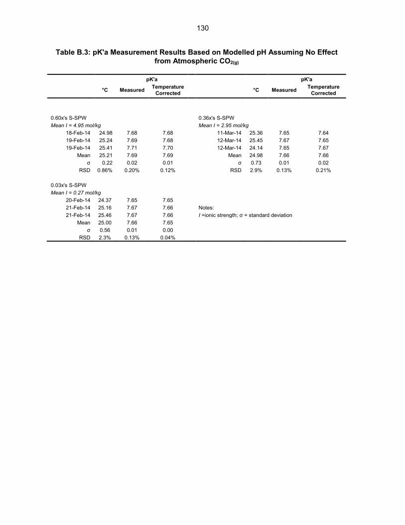
130


pK'a

pK'a


Corrected

0.60x's S-SPW

0.36x's S-SPW


Mean I = 2.95 mol/kg 18-Feb-14 24.98 7.68 7.68

11-Mar-14 25.36 7.65 7.64

19-Feb-14 25.24 7.69 7.68

12-Mar-14 25.45 7.67 7.65 19-Feb-14 25.41 7.71 7.70

12-Mar-14 24.14 7.65 7.67

Mean 25.21 7.69 7.69

Mean 24.98 7.66 7.66 σ 0.22 0.02 0.01

σ 0.73 0.01 0.02

RSD 0.86% 0.20% 0.12%

RSD 2.9% 0.13% 0.21%

0.03x's S-SPW Mean I = 0.27 mol/kg

20-Feb-14 24.37 7.65 7.65 21-Feb-14 25.16 7.67 7.66

Notes: 21-Feb-14 25.46 7.67 7.66

I =ionic strength; σ = standard deviation

Mean 25.00 7.66 7.65 σ 0.56 0.01 0.00 RSD 2.3% 0.13% 0.04%

improvements in methodologies for radiographic measurement

Documents