improved failure detection with higher degree of

Improved failure detection with higher degree of statistical confidence

JOSEFINE TARVAINEN

Master of Science Thesis

Stockholm, Sweden 2015

Examensarbete MMK 2015:109 MKN 156

Förbättrad utfallsdetektering med hög konfidensgrad

Josefine Tarvainen

Godkänt

2015-06-11

Examinator

Ulf Sellgren

Handledare

Ulf Sellgren

Uppdragsgivare

Scania CV AB

Kontaktperson

Mats Furukrona

Sammanfattning Detta examensarbete har utförts på uppdrag av Scania CV AB i Södertälje. Scania CV AB är ett

globalt företag som tillverkar tunga fordon, såsom lastbilar och bussar. Vid utveckling av en

växellåda, är ett livslängdsprov genomfört för att upptäcka typiska fel, t.ex. skadade kugghjul eller

lager. Idag används två system, STP och delta-ANALYSER, för att upptäcka fel.

STP har utvecklats av Scania CV AB, och det används för att mäta vibration, oljetryck, temperatur,

etc. Delta-ANALYSER är framtaget av Reilhofer. Det är ett mätsystem som detekterar fel i

växellådan genom att jämföra vibrationer med en referens. Det största problemet är att dessa

system är tidskrävande. Målet är att förkorta provtiden men fortfarande erhålla tydliga resultat och

i ett tidigt stadium erhålla en rapportering av skador på lager och kugghjul. Det är inte möjligt att

accelerera proven eftersom provriggarna redan är kraftigt accelererad.

Målet med examensarbetet är att göra en undersökning av befintliga system som kan tänkas vara

användbara för tidig detektering av utfall kopplat till en viss storlek och kunna isolera felkällan till

en viss del av växellådan.

I detta examensarbete har flera tekniker för detektering av skador identifierats: vibration,

termografi, akustisk emission, ultraljud, oljeanalys, etc. Efter en intern diskussion så valdes det att

kombinera två olika tekniker, oljeanalys och vibration. Flera olika företag som jobbar med

oljeanalys demonstrerade sina system. Fördelar och nackdelar diskuterades och det valdes att gå

vidare med en oljepartikelsensor, OPCom FerroS, från ARGO HYTOS, som med hjälp av en

magnet i oljeflödet kan detekterar oljepartiklar.

Det slutgiltiga systemet för detektering av skador blev en kombination av OPCom FerroS och

Scanias nuvarande system: delta-ANALYSER och STP. Det utvecklade detekteringssystemet

utvärderades med de ställda kraven och det påvisade att systemet uppfyller 22 av de 33

testade kraven. Alla krav kunde inte verifieras och kräver vidare undersökningar och tester.

Nyckelord: växellåda, vibration, kugghjul, lastbil

Master of Science Thesis MMK 2015:109 MKN 156

Improved failure detection with higher degree of statistical confidence

Josefine Tarvainen

Approved

2015-06-11

Examiner

Ulf Sellgren

Supervisor

Ulf Sellgren

Commissioner

Scania CV AB

Contact person

Mats Furukrona

Abstract This master thesis has been performed by a request from Scania CV AB in Södertälje. Scania CV

AB is a global company manufacturing heavy vehicles, such as busses and trucks. When

developing a gearbox, an endurance test is made that shows failures, such as damaged gears or

bearings. STP and delta-ANALYSER are used to discover this kind of failure.

STP is developed by Scania CV AB, and it measures the vibration, oil pressure, temperature, etc.

delta-ANALYSER is developed by Reilhofer. It is a measuring system that detects failures in the

gearbox by comparing the vibrations with a reference. The main issue is that these tests are time

consuming. The goal is to cut time and still be able to follow the results more accurately and in an

early stage receive failure reports from bearings and gears. Accelerate the tests is not possible,

because the test-rig is already heavily accelerated.

The purpose of the thesis is to investigate existing methods for a more precise detection of a

damage that has reached a certain size, also be able to isolate the source of a defect to a specific

gear.

In this thesis project different methods for detection of damages has been identified: vibration,

thermography, acoustic emission, ultrasonic, oil analysis, etc. After an internal discussion, a

combination of two methods: oil analysis and vibration, were chosen. Companies demonstrated

their oil analysis systems. Advantages and disadvantages were discussed and it was decided to

continue with an oil particle sensor, OPCom FerroS, from ARGO HYTOS, that detect the oil

particles with a magnet in the flow of oil.

The final system for detection of damages is a combination of OPCom FerroS and Scania’s current

system: delta-ANALYSER and STP. The developed detection system was evaluated by the set

system requirements, showing that the system meet 22 of the 33 tested requirements. All

requirements could not be verified and needs more investigation and tests.

Keywords: Gearbox, Vibration, Gear, Truck

FOREWORD

This master thesis has been carried out for 20 weeks. The project is limited to a period that starts

the 13th of April until the 30th of August and it will take place at the transmission development,

gearbox, department (NTBG) at Scania CV AB in Södertälje. I would like to use this section to

thank all the people who have helped and supported me during the thesis.

I would like to thank my supervisor at KTH, Ulf Sellgren, for his support and expertise, and also

the NTBG department at Scania for providing me with the opportunity of conducting my master

thesis. I would like to give a special thanks to my supervisor at Scania, Mats Furucrona, who has

supported me with information, feedback, direction and ideas during the thesis project. I also

would like to thank the interviewees who provided me with background information which

enabled me to develop a process for early detection of failure.

Another thanks to my family, who has supported and encourage me during the thesis work.

Josefine Tarvainen

Stockholm, August 2015

NOMENCLATURE

This part of the report consist of the abbreviations used in this master thesis.

Abbreviations

AE Acoustic Emission

APC Automated Particle Counting

CAD Computer Aided Design

CAE Computer Aided Engineering

CAN Control Area Network

CM Condition monitoring

CPS Creative Problem Solving

cps cycles per second

DFT Discrete Fourier Transform

EMD Empirical Mode Decomposition

EMF Electromotive Force

FFT Fast Fourier Transformation

FMEA Failure Mode Effect Analysis

FT Fourier Transformation

Hz Hertz

ICE Internal Combustion Engine

IMF Intrinsic Mode Function

IR Infrared

kHz Kilohertz

MHz MegaHertz

MPI Magnetic Particle Inspection

NDE Nondestructive Evaluation

NDT Nondestructive Testing

OPC OptiCruise

OSHA Occupational Safety and Health Administration

PLM Product Lifecycle Management

rpm Revolutions per minute

STFT Short Time Fourier Transform

STP Scania Test Plattform

TAN Total Acid Number

TBN Total Base Number

TCU Transmission Control Unit

TE Transmission Error

TEDS Transducer Electronic Data Sheet

THT Teager-Huang transform

TKEO Teager Kaiser Energy Operator

WT Wavelet Transform

WVD Wigner-Ville distribution

TABLE OF CONTENTS

INTRODUCTION ............................................................................................................................................ 1

1.1 BACKGROUND ..................................................................................................................................................... 1

1.2 PURPOSE AND DELIVERABLES .................................................................................................................................. 2

1.3 DELIMITATIONS ................................................................................................................................................... 2

1.4 METHOD ............................................................................................................................................................ 3

FRAME OF REFERENCE ................................................................................................................................. 7

2.1 GEARBOX ........................................................................................................................................................... 7

2.2 TEST-RIG .......................................................................................................................................................... 17

2.3 WEIBULL ANALYSIS ............................................................................................................................................. 21

2.4 CONDITION MONITORING (CM) ........................................................................................................................... 22

2.5 VIBRATION ....................................................................................................................................................... 23

2.6 THERMOGRAPHY ............................................................................................................................................... 44

2.7 OIL ANALYSIS .................................................................................................................................................... 46

2.8 EDDY CURRENT TESTING ...................................................................................................................................... 54

2.9 ULTRASONIC ..................................................................................................................................................... 57

2.10 RADIOGRAPHY TESTING .................................................................................................................................. 59

2.11 ACOUSTIC EMISSION ...................................................................................................................................... 60

2.12 MAGNETIC PARTICLE INSPECTION ..................................................................................................................... 63

THE PROCESS .............................................................................................................................................. 65

3.1 PHASE 1 - PROJECT PLANNING .............................................................................................................................. 65

3.2 PHASE 2 – RESEARCH ......................................................................................................................................... 76

3.3 PHASE 3 - SYSTEM EVALUATION ............................................................................................................................ 85

3.4 PHASE 4 - DETAIL DESIGN .................................................................................................................................... 98

RESULTS .................................................................................................................................................... 102

4.1 FINAL SYSTEM ................................................................................................................................................. 102

4.2 OPCOM FERROS – ARGO HYTOS..................................................................................................................... 102

4.3 MEASURING PRINCIPLE ..................................................................................................................................... 102

4.4 DESIGN CHARACTERISTICS .................................................................................................................................. 104

4.5 SENSOR CONNECTION ....................................................................................................................................... 104

4.6 DATA DISPLAY AND PROCESSING ......................................................................................................................... 105

4.7 TECHNICAL SPECIFICATION ................................................................................................................................. 107

DISCUSSION AND CONCLUSION ................................................................................................................ 109

5.1 DISCUSSION .................................................................................................................................................... 109

5.2 CONCLUSION .................................................................................................................................................. 111

FUTURE WORK .......................................................................................................................................... 112

6.1 FUTURE WORK ................................................................................................................................................ 112

REFERENCES ....................................................................................................................................................... 113

APPENDICES ....................................................................................................................................................... 121

TABLE OF FIGURES

Figure 1. The CPS process (Puccio, et al., 2011) ............................................................................ 3

Figure 2. The project process .......................................................................................................... 4

Figure 3. Gearbox location (Scania, 2011) ..................................................................................... 7

Figure 4. Gearbox GR905 cutaway (Scania, 2015) ........................................................................ 8

Figure 5. The route of transmission power through the gearbox .................................................... 8

Figure 6. Gears (Scania, 2012) ........................................................................................................ 9

Figure 7. The external components of a gearbox without retarder: 1: Front part, 2a: Middle part

for GR 875, GRS 895 and GRSO 895, 2b: Middle part for GR 905, GRS 905, GRSO 905 and

GRSO 925, 3a: End part, 4b: End part with retarder (Karlsson, 2015) .......................................... 9

Figure 8. Synchronizing parts (Karlsson, 2015) ........................................................................... 10

Figure 9. Synchronizing process, 1: The gearbox, 2: Synchronization, 3: The route of power

transmission (Karlsson, 2015) ....................................................................................................... 10

Figure 10. Range. 1: Main shaft, 2: Main shaft gear, 3: Ring gear, 4: Planetary gear, 5: Clutch

pack, 6: Locking gear, 7: Planet carrier, 8: synchronizing cones, 9: Sun gear (Karlsson, 2015) . 11

Figure 11. Low and high range (Karlsson, 2015) ......................................................................... 11

Figure 12. The routes of transmission power for low and high split for each gear (Karlsson, 2015)

....................................................................................................................................................... 12

Figure 13. Lubrication system, 1: Oil pump, 2: Dump valve, 3: Oil filter, 4: Suction strainer

(Karlsson, 2015) ............................................................................................................................ 13

Figure 14. Filter (Ringholm, 2004) ............................................................................................... 13

Figure 15. Oil filter middle part, Red line: Oil (out), Green line: Oil (in) .................................... 14

Figure 16. The amount of metal particle in the gearbox after an endurance test .......................... 14

Figure 17. Different types of misalignments (Mobley, 2001, p. 797)........................................... 15

Figure 18. Spur Gear - Pressure angle (Randall, 2010, p. 41) ...................................................... 16

Figure 19. The test-rig (Prytz, 2008) ............................................................................................. 17

Figure 20. Test-rig: T17 ................................................................................................................ 18

Figure 21. Clamping device (Prytz, 2008) .................................................................................... 19

Figure 22. A schematic illustration of the oil system: 1: Heat-exchanger, 2: Quick connection, 3:

Temperature sensor, 4: Temperature sensor, 5: Pressure sensor, 6: Quick connection, 7: Level

sensor. (Gustavsson, 2006) ............................................................................................................ 20

Figure 23. Oil system: 1: Quick connection, 2: Oil plug, 3: Oil temperature sensor (TV01), 4: Oil

level sensor, 5: Temperature sensor, Pump for waste oil: 6: Valve 1, 7: Valve 2, 8: Valve 3.

(Gustavsson, 2006) ........................................................................................................................ 20

Figure 24. The Weibull analysis process (Abernethy, et al., 1983, p. 3) ...................................... 21

Figure 25. Description of the result (Abernethy, et al., 1983, p. 4) .............................................. 21

Figure 26. The condition monitoring process ............................................................................... 22

Figure 27. Single degree-of-freedom (Undamped system) (Mohanty, 2015, p. 14) ..................... 24

Figure 28. Single degree-of freedom (Damped system) (Mohanty, 2015, p. 14) ......................... 24

Figure 29. Diagram a) illustrates the magnitude response of a harmonically forced damped

oscillation, diagram b) illustrates the phase between response and force of a damped oscillator

(Mohanty, 2015, pp. 16-17) .......................................................................................................... 26

Figure 30. Simple theoretical vibration curve (Mobley, 2002, p. 117) ......................................... 27

Figure 31. An example of a time-domain vibration profile (Mobley, 2002, p. 119) .................... 27

Figure 32. An example of a frequency-domain vibration profile (Mobley, 2002, p. 120) ........... 28

Figure 33. The relationship between the time-domain and the frequency-domain (Mobley, 2002,

p. 150) ............................................................................................................................................ 28

Figure 34. Difference between the local fault and the distributed fault (Randall, 2010, p. 45). ... 33

Figure 35. Frequency Spectrum and Order Spectrum for a Gear Wheel (Discom, 2012) ............ 35

Figure 36. Common Defects of a Gear Wheel (Discom, 2012) .................................................... 36

Figure 37. FFT plot of a bearing with a first order damage frequency (Vibrationschool, 2015) .. 37

Figure 38. Outer race damage (Ludeca, 2011) .............................................................................. 37

Figure 39. Bearing symbol definition (Lindholm, 1995, p. 47) .................................................... 38

Figure 40. Displacement probe and the system of the signal condition (Mobley, 2001, p. 50) .... 39

Figure 41. Schematic Diagram of a measurement device for the velocity: 1. Pickup case, 2. Wire

out, 3. Damper, 4. Mass, 5. Spring, 6. Magnet. (Mobley, 2001, p. 52) ........................................ 40

Figure 42. A piezoelectric accelerometer (PCB, 2015) ................................................................ 40

Figure 43. Cymbal piezoelectric composite transducer (Denghua, et al., 2010) .......................... 41

Figure 44. Permanent transducer mounting (Mobley, 2002, p. 158). ........................................... 42

Figure 45. Thermography (Supervision, 2014) ............................................................................. 44

Figure 46. The process of Infrared Scanning (Saeed, 2008) ......................................................... 45

Figure 47. Wear particles (Peng & T.B, 1999) ............................................................................. 46

Figure 48. Relationship between the generated particles and the condition of the component

(Bogue, 2013) ................................................................................................................................ 47

Figure 49. Difference between online, inline and offline monitoring (Gebarin, 2003) ................ 48

Figure 50. A schematic illustration of the light blockage particle count (Lubrication, 2002) ...... 49

Figure 51. A schematic illustration of the light scattering particle count (Lubrication, 2002) ..... 49

Figure 52. The pore blockage particle counting technique (Williamson, 2009) ........................... 50

Figure 53. Emission spectrometry (Dahunsi, 2008) ...................................................................... 51

Figure 54. Atomic absorption spectrographic (Dahunsi, 2008) .................................................... 51

Figure 55. Direct-Reading Ferrograph monitor (Laboratories, 2003) .......................................... 52

Figure 56. Oil Classification table (CJC, 2015) ............................................................................ 53

Figure 57. An eddy current probe used for detection of the character of conductive materials.

Figure (a) show the response of the probe in the absence of conductive material and figure (b)

show the response of the probe in the presence of conductive material (Shull, 2002, p. 260). .... 54

Figure 58. A diagram of the EC system (DeVries, 2013). ............................................................ 55

Figure 59. Shape of the response curve (Shull, 2002, p. 227) ...................................................... 55

Figure 60. EC inspection system (Shull, 2002, p. 221) ................................................................. 56

Figure 61. The process of ultrasonic testing (MaterialsScience2000, 2014) ................................ 57

Figure 62. A schematic illustration of radiographic testing (Davies, 1998, p. 121) ..................... 59

Figure 63. Values of the electromagnetic spectrum (Shull, 2002, p. 345) .................................... 59

Figure 64. The process of Acoustic Emission monitoring (Hellier, 2003, p. 536) ....................... 61

Figure 65. Illustration of the response of the AE sensor (Shull, 2002, p. 375) ............................. 62

Figure 66. The magnetic inspection process (MaterialScience2000, 2014) ................................. 63

Figure 67. Magnetic particle inspection of a gear wheel (MaterialScience2000, 2014) ............... 63

Figure 68. Circular magnet (Shull, 2002, p. 194) ......................................................................... 64

Figure 69. Phase 1 – Project Planning ........................................................................................... 65

Figure 70. The sensors for the control/measuring and regulation system ..................................... 66

Figure 71. Control panel in the control room: 1: Emergency stop, 2: Gear shifting unit, 3:

Watchdog, 4: RPM rear machine, 5: Torque rear machine, 6: RPM front machine, 7: Torque front

machine. ........................................................................................................................................ 67

Figure 72. The STP-states (Einarsson, 2011) ................................................................................ 67

Figure 73. Test information window (Einarsson, 2011) ............................................................... 68

Figure 74. User specified monitoring ............................................................................................ 69

Figure 75. Test results for the third gear high split: MPPT01 = Oil temperature into the gearbox,

TV01 = Oil temperature out of the gearbox, PV01 = Oil pressure, NX01 = Vibration, NX01 gräns

= Vibration limit ............................................................................................................................ 70

Figure 76. Propagation of the sound (Reilhofer, 2014) ................................................................. 71

Figure 77. Piezoelectric sensor ...................................................................................................... 71

Figure 78. A schematic illustration of the system ......................................................................... 71

Figure 79. Trendindex (Reilhofer, 2014) ...................................................................................... 72

Figure 80. Waterfall diagram (Reilhofer, 2014) ........................................................................... 73

Figure 81. Trendindex: Planetary gear test, third gear high split damage progression ................. 73

Figure 82. Waterfall diagram: Planetary gear test, third gear high split ....................................... 74

Figure 83. Order Calculator .......................................................................................................... 74

Figure 84. Phase 2 – Research ...................................................................................................... 76

Figure 85. Function tree ................................................................................................................ 78

Figure 86. Simplified Pugh Matrix ............................................................................................... 83

Figure 87. Condition monitoring methods’ pre-warning time of failure (Parker, 2014) .............. 84

Figure 88. Phase 3 – System evaluation ........................................................................................ 85

Figure 89. SKF - Multilog Online System IMx-W (SKF, 2003) .................................................. 86

Figure 90. eMDSS (e-Maintenance Decision Support System) .................................................... 88

Figure 91. The icountOS (IOS) particle counter (Parker, 2014) ................................................... 89

Figure 92. The laser diode optical detection measuring process (Parker, 2014) .......................... 89

Figure 93. Metallic Wear Debris Sensor (Kittiwake, 2015) ......................................................... 90

Figure 94. Metallic Wear Debris Sensor in action (Kittiwake, 2015) ........................................... 90

Figure 95. Number of particles (Kittiwake, 2015) ........................................................................ 90

Figure 96. Wearscanner (Prüftechnik, 2009) ................................................................................ 91

Figure 97. The eddy current principal (Prüftechnik, 2008) ........................................................... 91

Figure 98. OPCom Ferros (ARGO-HYTOS, 2015) ...................................................................... 92

Figure 99. OPCom Particle Monitor (ARGO-HYTOS, 2015) ...................................................... 92

Figure 100. PCM400 Cleanliness monitor and an example of a test result (Colly, 2011) ............ 93

Figure 101. Trender software (Colly, 2011) ................................................................................. 93

Figure 102. QFD ........................................................................................................................... 95

Figure 103. Oil analysis systems (QFD results) ............................................................................ 96

Figure 104. Oil particles distribution ............................................................................................ 97

Figure 105. Diagram of the oil particle distribution ...................................................................... 97

Figure 106. Phase 4 – Detail design .............................................................................................. 98

Figure 107. Concept 1 – Oil flow chart ......................................................................................... 98

Figure 108. Oil temperature results from endurance test .............................................................. 99

Figure 109. Concept 2 – Oil flow chart ......................................................................................... 99

Figure 110. Concept 3 – Oil flow chart ....................................................................................... 100

Figure 111. FMEA ...................................................................................................................... 100

Figure 112. Final failure detection process ................................................................................. 102

Figure 113. OPCom FerroS (ARGO-HYTOS, 2015) ................................................................. 102

Figure 114. Measuring principal (Fredenwall, 2015) ................................................................. 103

Figure 115. Cleaning process (Fredenwall, 2015) ...................................................................... 103

Figure 116. Measurements (ARGO-HYTOS, 2015) .................................................................. 104

Figure 117. Oil cooling system ................................................................................................... 104

Figure 118. Flow chart ................................................................................................................ 105

Figure 119. LubMon PClight (ARGO-HYTOS, 2015) ............................................................... 105

Figure 120. A schematic illustration of the communication between sensor and software (ARGO-

HYTOS, 2015) ............................................................................................................................ 106

Figure 121. LubMon Connect (ARGO-HYTOS, 2015) ............................................................. 106

TABLE OF TABLES

Table 1. The Purpose of the Four Stages (Puccio, et al., 2011) ...................................................... 3

Table 2. Scania’s gearboxes ............................................................................................................ 7

Table 3. Specifications of the front machine and the rear machine (Prytz, 2008) ........................ 18

Table 4. Weibull Risk Forecast (Abernethy, et al., 1983, p. 7) ..................................................... 22

Table 5. Failure modes and its features (phmsociety, 2009) ......................................................... 32

Table 6. Items’ sizes (CJC, 2015) ................................................................................................. 53

Table 7. System Requirements ...................................................................................................... 76

Table 8. Advantages and disadvantages of the methods ............................................................... 79

Table 9. Suppliers and their condition monitoring methods ......................................................... 81

Table 10. Chosen suppliers and their systems............................................................................... 85

Table 11. SKF vs. delta-ANALYSER .......................................................................................... 87

Table 12. Comparison of Systems ................................................................................................. 93

Table 13. Technical data (ARGO-HYTOS, 2015) ...................................................................... 106

Table 14. OPCom FerroS properties ........................................................................................... 107

Table 15. System Requirements .................................................................................................. 109

TABLE OF APPENDICES

APPENDIX A: THESAURUS........................................................................................................ 1

APPENDIX B: RISK-ANALYSIS ................................................................................................. 2

APPENDIX C: INTERVIEWEES .................................................................................................. 3

APPENDIX D: PERSONA ............................................................................................................. 4

APPENDIX E: SYSTEM REQUIREMENTS ................................................................................ 5

1

INTRODUCTION

The following report is a part of a master thesis project (30 credits) at advanced level within

machine design. The thesis project is performed at the transmission development, gearbox,

department (NTBG) at Scania CV AB in Södertälje. It is performed by a student at the Royal

Institute of Technology (KTH), during the period April-August. The project is supervised by Mats

Furukrona at Scania CV AB and Ulf Sellgren who is responsible for the master’s track in Machine

Design. This chapter describes the background, the purpose, the limitations and the method used

in the presented project.

1.1 Background

Scania CV AB is a manufacture of heavy trucks and buses, founded in Sweden 1891. With its

presence in 100 countries around the world it is a global company. The head office is located in

Södertälje. Scania CV AB offers many different gear changing variants: fully manual, automatic

gear changing system with clutch pedal, fully automatic gear changing system without clutch pedal

and finally an automatic gearbox.

A gearbox is an important component of the heavy trucks, because of its effect on the vehicle. It

is a technical advanced system, which must be able to operate in tough environments so quality

and functionality are very important.

When developing a gearbox, a functionality verification is made to guarantee that the new gearbox

meet the requirements. When validating the gearbox, it is endurance tested in a test-rig, where the

gearbox is connected to two electrical motors. The endurance test is designed to test the life of the

gearbox during operating conditions.

The operating conditions are similar to the ones that the gearbox is subjected to in the truck, such

as lubrication, temperature, incline angle etc. The environmental factors such as dust, road induced

vibrations, water spray are not implemented because they are not considered to impact test life.

The testing time for the gearboxes differ, but some are tested up to 1800 hours. The tests are

heavily accelerated by removing load levels and corresponding load time that does not contribute

to failure according to Palmgren-Miner linear damage hypothesis, it is not feasible to accelerate

them further without risking irrelevant failure modes.

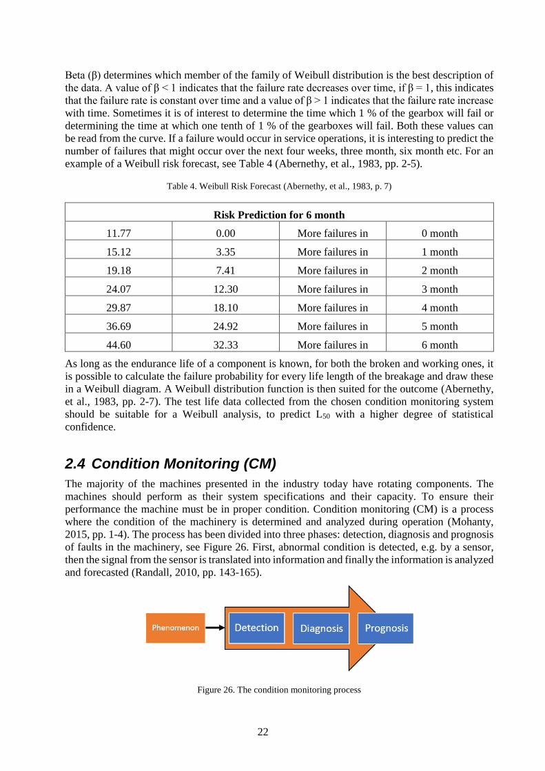
Condition monitoring (CM) is a process of monitoring a parameter of condition in the machinery

to receive an indication of a developing fault, such as a crack in a gear, so appropriate action can

be taken before it causes catastrophic failure. Scania CV AB is using STP and delta-ANALYSER

to analyze the result from the endurance test in real-time. The STP system is developed by Scania

CV AB and measures vibrations, temperature and torque etc.

The latest system installed is delta-ANALYSER, developed by Reilhofer, which measure the

structure-born noise by using a piezoelectric sensor mounted on the gearbox. It detects failure by

comparing the gearbox vibration with a developed reference. The main objective with delta-

ANALYSER was to be able to stop the test when a damage on the gears or/and bearings have

reached a size defined by Scania CV AB. This would shorten the test time and more precise

detection surface fatigue failures. It has been shown that this is difficult to accomplish, and the

results are not accurate enough.

2

1.2 Purpose and deliverables

The purpose of the thesis project is to reduce the testing time for development projects by

investigating methods that have potential for early detection of failures. This means that the

endurance test should stop in an earlier stage of a damage of a component, e.g. spalling or pitting,

has reached a specified size of the surface. Through experience, Scania CV AB has been able to

set acceptance criteria levels for the gears and bearings.

The failure detection should be precise enough to indicate a failure according to the acceptance

criteria and the results should be suitable for Weibull Analysis.

The purpose of the project has been divided into two sub goals:

Investigate and present different condition monitoring methods.

Choose the best solution on how to improve detection of failures.

1.3 Delimitations

The master thesis (30 credits) lasts for 20 weeks, about 40 hours per week. The project is limited

to a period that starts the 13th of April until the 30th of August and it take place at the transmission

development, gearbox, department (NTBG) at Scania CV AB in Södertälje.

Limitations were made in the beginning of the project, in order to meet the allowed timeframe of

the thesis project.

The thesis is limited to investigate and study existing failure detection systems.

The research is not narrowed to only systems for truck gearboxes, to make the research as

wide as possible.

Only manual gearboxes is studied during the project, because the testing procedure is

different for a manual gearbox and an automatic and there is not enough time to investigate

both.

The integrity of the gearbox must be unaffected in terms of function and strength.

Tooth breakage is not taken in account, because this is not considered as a normal failure

mode at the used torque levels and are usually caused by material defects such as inclusion

or incorrect hardness.

The failure detection should be precise enough to indicate a failure according to acceptance

criterias set by Scania CV AB through experience.

Only online and inline systems are investigated, not offline systems.

The results from the failure detection solution should be suitable for Weibull analysis.

No tests of different condition monitoring methods is performed during the thesis and the

result is therefore only derived from theoretical basis. Meeting with the suppliers and

studying of the data sheet of the different system is performed as a complement.

The result of the thesis project is presented, both as a written technical report and an oral

presentation.

3

1.4 Method

The initial methodology of the thesis work consists of a thorough research in order to secure a

broad base of knowledge of the subject. The information from the research are then used for

formulate limitations and goals which is the base of the system requirements specification.

Condition monitoring methods and solutions on the market are investigated and studied and with

support of development tools, evaluated internally which results in a final solution. The process,

methodology and tools used to ensure the quality of this thesis project is described below.

1.4.1 General method

The approach used for this project is based on the model for Creative Problem Solving (CPS),

which is a method developed by Alex Osborn and Dr. Sidney J. Parnes. This approach has been

used since it was developed in the 1950s to generate solutions to problems in a more structured

way. The process of problem solving consists of four stages and these stages starts with a broad

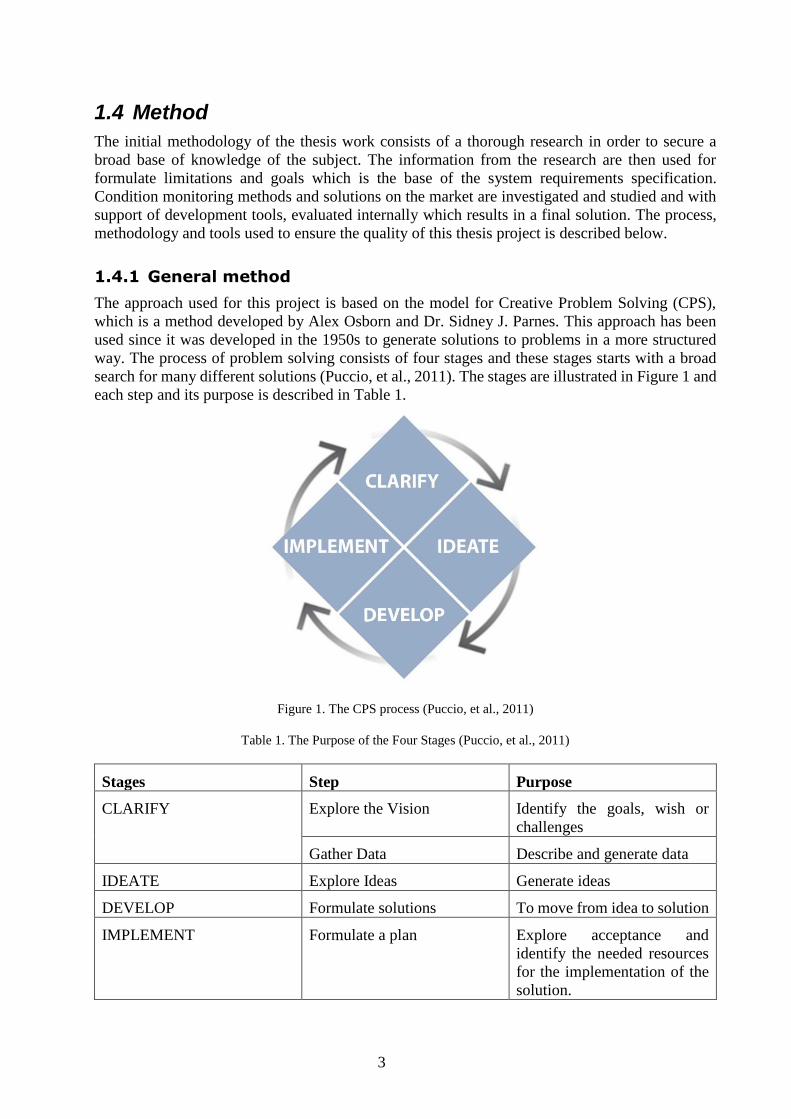
search for many different solutions (Puccio, et al., 2011). The stages are illustrated in Figure 1 and

each step and its purpose is described in Table 1.

Figure 1. The CPS process (Puccio, et al., 2011)

Table 1. The Purpose of the Four Stages (Puccio, et al., 2011)

Stages Step Purpose

CLARIFY Explore the Vision Identify the goals, wish or

challenges

Gather Data Describe and generate data

IDEATE Explore Ideas Generate ideas

DEVELOP Formulate solutions To move from idea to solution

IMPLEMENT Formulate a plan Explore acceptance and

identify the needed resources

for the implementation of the

solution.

4

Some modifications of the CPS process have been done to fit this project. The thesis project is

divided into four phases, to guide the development of the failure detection solution. Every phase

consist of general methods and development tools, to ensure the quality of the result. The tools

and methods follow the guidelines presented by Ulrich & Eppinger (2012) and Ullman (2010).

These methods are designed for product development, but are also applicable for system

development. Figure 2 describe the process of the project and also the content of each phase.

Figure 2. The project process

1.4.2 The data collection methodology

Most of the data are gathered by different internet sources and several unstructured interviews,

sources, which are described further below.

LITERATURE

The first part of the thesis consists of an extensive study of literature. A lot of the information is

collected through various data bases, such as KTHB Primo, IEEE Xplore and Scopus, and

information from supplier and interviews. During the literature study it is important to only use

information from reliable sources, e.g. books and articles where the author is trustworthy not use

secondary sources if possible and try to not use sources older than fifteen years. It is important to

understand that the suppliers from the companies are selling, which means that they are unlikely

to present the downsides of the systems.

INTERVIEWS

Interviews are not following a strict list of questions, more like a conversation. The respondent of

the interviews have the possibility to explain their thoughts and views and also talk about subject

that they finds relevant for this subject during the interview. For the interviewees see Appendix C.

QUANTITATIVE AND QUALITATIVE METHOD

Gathering, sorting and analyzing a large amount of data is called quantitative research. While

qualitative research is when focusing on a small amount of information (Kaplan & Duchon, 1988).

The main focus is to find information about systems for condition monitoring and to gather

information and analyze it deeply. During the collecting of information about the suppliers and

information about other companies and their solution, a quantitative research is done.

5

1.4.3 The process development methodology

The methodology of the development of a process that can improve the failure detection illustrated

in Figure 2 is described below.

PHASE 1 – PROJECT PLANNING

Phase 1 is the planning phase and the purpose of this phase is to understand the aim of the project.

Planning

A Gantt chart is established for the scheduling of the project, because it gives a good overview of

the project, and to be aware of the risk and to know how to solve these a risk analysis is written,

see Appendix B.

Literature Study

The project planning is based on the literature study, to increase the knowledge of the manual

gearbox, test-rig, current system used by Scania CV AB and general about condition monitoring.

The literature study is important to gain knowledge to improve the methodology of the thesis

project.

Pre-study

A pre-study is appropriate to understand the problem and to define the limitations of the project.

In the pre-study, the current systems used by Scania CV AB, delta-ANALYSER and STP, are

investigated.

PHASE 2 - RESEARCH

The research phase consists of searching for methods that can detect failures in a gearbox. All

methods are investigated, and the search is not narrowed to only truck gearboxes, to make the

research as wide as possible. The information from phase 1 is used as a base for the research. The

second phase consists of interviews with the staff at Scania CV AB office in Södertälje. This is

made to understand the specifications needed of the system and the advantages and disadvantages

of current system, delta-ANALYSER and STP. It results in a system specification, which the

system must fulfil to be considered implementable. A research of existing product on the market

and also possible solution are investigated during this phase.

Persona

A persona is made to understand the need of the customer, which is a representation of a specific

group of people with common product requirements, a market segment. Doing a persona gives a

better understanding of the chosen target. The information to the persona is gathered from

interviews with the employees at Scania.

System Requirements Specification

The system requirements specification list the requirements of the system set by the user, costumer

and the supplier. According to Ullman (2010), most of the requirements should be measureable to

avoid subjective definitions. The final system requirements specification is used as a base for the

evaluation of the systems (Ulrich & Eppinger, 2012).

Function tree

The purpose and the functions of the systems must be clarified before the identification of existing

condition monitoring solutions can begin. A convenient method to clarify it, is to divide the

6

function into sub-functions in a function tree (Ulrich & Eppinger, 2012). A function tree is

established from the specified requirements.

Benchmarking

A benchmarking is performed to identify the systems that exist on the market. The advantages and

the disadvantages of the systems are studied and evaluated. These are identified by interviews with

suppliers and employees at Scania.

Pugh Matrix

The Pugh matrix allows a comparison of how well each condition monitoring method meet the

requirements set in the beginning of the project. Each method is compared to a reference, which

in this case is the current solution, used by Scania: delta-ANALYSER and STP. The methods are

listed in a table and were weighted: (+) if the method is better than the reference, (0) the same and

(-) if the reference is better than the method. The purpose of the matrix is to evaluate different

methods. The result from the Pugh matrix and the opinions of Scania is used for deciding the most

appropriate condition monitoring method (Ulrich & Eppinger, 2012).

PHASE 3 – SYSTEM EVALUATION

In phase 3 the economical and functional aspects are considered when choosing the most

appropriate system within the chosen method. The supplier of the systems are contacted for a

demonstration of their systems. The systems are evaluated in an evaluation matrix, by the

knowledge gained from interviews and the literature study. The aim of phase 3 is to have at least

one final system. The systems are evaluated in a QFD, to ensure the final result.

QFD – Quality Function Deployment

The Quality Function Deployment (QFD) is established from the customer requirements, the

vertical factors, and the functional requirements, the vertical factors. The functional and the

customer requirements are related in the QFD. The matrix also allows a comparison of the found

systems (Ulrich & Eppinger, 2012).

PHASE 4 – DETAIL DESIGN

When the final system is decided and verified, then the development of the system is continued in

detail. A proposal of a layout of the final system is made.

Risk analysis

The safety risks of the system are evaluated in a Failure Mode Effect Analysis (FMEA). The tool

is used for investigating potential failures of the system, the reason of these and also the effects.

The result of the FMEA is then be used for deciding recommended actions for each potential

failure (Ulrich & Eppinger, 2012).

7

FRAME OF REFERENCE

This chapter presents the theoretical reference frame that is necessary for the performed research.

2.1 Gearbox

The main purpose of the gearbox is to change the gear ratio, depending on the requirements of

speed and power, which is achieved by using different combinations of gears. A gearbox is a torque

or rotational speed converter. The gearbox is positioned between the front wheels and behind the

engine, see Figure 3 (Scania, 2012).

Figure 3. Gearbox location (Scania, 2011)

In the transmission of vehicles the gearbox controls the power transferred from the engine to the

wheels of the vehicle. The transmission system control the fuel and power in the vehicle. The

performance of the transmission is dependable of gear efficiency, noise and shift comfort during

gear change. The three different types of transmission systems are manual, automatic and electro-

mechanical transmission system (Bedmar, 2013). Scania CV AB offers four different kinds of

gearboxes: fully manual, automatic gear changing system with clutch pedal called Scania

OptiCruise, fully automatic gear changing system without clutch pedal called Scania OptiCruise

and an automatic gearbox (Scania, 2012). Scania has a module system, which makes it possible to

combine the components of a gearbox based on the customers’ needs and desires. A list of the

gearboxes manufactured at Scania is presented in Table 2, where G stands for gearbox, GR stands

for Gearbox Range and GRS for Gearbox Range Split. The gearbox called GRSO is an overdrive

gearbox, which means that it has a gear with a gear ratio less than 1. For an example of a manual

gearbox from Scania see Figure 4 (Karlsson, 2015).

Table 2. Scania’s gearboxes

Name Number of gears

GR 875 8

GR 905 9

GRS 895, GRSO 895 12

GRS 905, GRSO 905, GRSO925 14

8

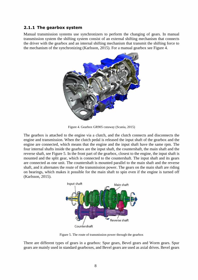
2.1.1 The gearbox system

Manual transmission systems use synchronizers to perform the changing of gears. In manual

transmission system the shifting system consist of an external shifting mechanism that connects

the driver with the gearbox and an internal shifting mechanism that transmit the shifting force to

the mechanism of the synchronizing (Karlsson, 2015). For a manual gearbox see Figure 4.

Figure 4. Gearbox GR905 cutaway (Scania, 2015)

The gearbox is attached to the engine via a clutch, and the clutch connects and disconnects the

engine and transmission. When the clutch pedal is released the input shaft of the gearbox and the

engine are connected, which means that the engine and the input shaft have the same rpm. The

four internal shafts inside the gearbox are the input shaft, the countershaft, the main shaft and the

reverse shaft, see Figure 5. In the front part of the gearbox, closest to the engine, the input shaft is

mounted and the split gear, which is connected to the countershaft. The input shaft and its gears

are connected as one unit. The countershaft is mounted parallel to the main shaft and the reverse

shaft, and it alternates the route of the transmission power. The gears on the main shaft are riding

on bearings, which makes it possible for the main shaft to spin even if the engine is turned off

(Karlsson, 2015).

Figure 5. The route of transmission power through the gearbox

There are different types of gears in a gearbox: Spur gears, Bevel gears and Worm gears. Spur

gears are mainly used in standard gearboxes, and Bevel gears are used as axial drives. Bevel gears

9

enable deflection of the transferred torque by 90°. While Worm gears often is used as axial drives

in special vehicles (Scania, 2012). For all the different types, see Figure 6.

Figure 6. Gears (Scania, 2012)

The spur gear is most common of these gears and it is the least expensive to manufacture. The

main idea of the spur gear is to make a connection between parallel shafts, where the rotation is in

opposite direction. The advantage of these gears is that they can be manufactured to close

tolerances. The bevel gear is mostly used for 90° drives, but also for other angles. A bevel gear is

always conical in shape, while the spur gear is typically cylindrical. Sets of bevel gears must have

the same angle pressure, tooth length and diametric pitch, which mean that they have to be

manufactured in pairs. Worm gears are used when a high-ratio speed reduction is needed. The

advantage of the worm gear is low wear. The wheel in a typical set of worm gears is often made

of bronze and the worm of hardened steel (Mobley, 2001, pp. 631-635).

The housing of the gearbox consist of three joined components: a front part attached to the engine,

an end part where the range is mounted and a middle part where the remaining gears are mounted.

The front and end part are made of aluminum, while the middle part is made of cast iron. The

external components is based on a module system and for a presentation of the components see

Figure 7. The middle part can be altered depending on the choice of gearbox, and some of the

gearboxes have a retarder mounted with the middle housing part instead of the end part. The

retarder is a brake that work as a complement to the ordinary braking system to increase the life

of the wheels’ breaking pads. A retarder is e.g. necessary for a truck driving in the Alps (Karlsson,

2015).

Figure 7. The external components of a gearbox without retarder: 1: Front part, 2a: Middle part for GR 875, GRS

895 and GRSO 895, 2b: Middle part for GR 905, GRS 905, GRSO 905 and GRSO 925, 3a: End part, 4b: End part

with retarder (Karlsson, 2015)

10

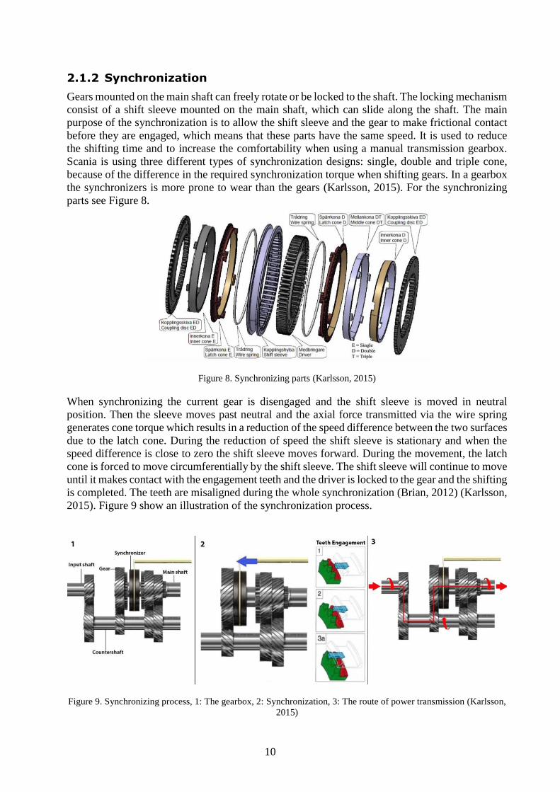
2.1.2 Synchronization

Gears mounted on the main shaft can freely rotate or be locked to the shaft. The locking mechanism

consist of a shift sleeve mounted on the main shaft, which can slide along the shaft. The main

purpose of the synchronization is to allow the shift sleeve and the gear to make frictional contact

before they are engaged, which means that these parts have the same speed. It is used to reduce

the shifting time and to increase the comfortability when using a manual transmission gearbox.

Scania is using three different types of synchronization designs: single, double and triple cone,

because of the difference in the required synchronization torque when shifting gears. In a gearbox

the synchronizers is more prone to wear than the gears (Karlsson, 2015). For the synchronizing

parts see Figure 8.

Figure 8. Synchronizing parts (Karlsson, 2015)

When synchronizing the current gear is disengaged and the shift sleeve is moved in neutral

position. Then the sleeve moves past neutral and the axial force transmitted via the wire spring

generates cone torque which results in a reduction of the speed difference between the two surfaces

due to the latch cone. During the reduction of speed the shift sleeve is stationary and when the

speed difference is close to zero the shift sleeve moves forward. During the movement, the latch

cone is forced to move circumferentially by the shift sleeve. The shift sleeve will continue to move

until it makes contact with the engagement teeth and the driver is locked to the gear and the shifting

is completed. The teeth are misaligned during the whole synchronization (Brian, 2012) (Karlsson,

2015). Figure 9 show an illustration of the synchronization process.

Figure 9. Synchronizing process, 1: The gearbox, 2: Synchronization, 3: The route of power transmission (Karlsson,

2015)

11

2.1.3 Range

The main shaft is connected to a planetary gear system, which is mounted on the output shaft. The

planetary gear system is known as the range. A planetary gear system consists of a sun gear in the

center, a ring gear and also several planet gears which rotate between these (Rohloff, 2015)

(Karlsson, 2015). For an illustration of the range and its position see Figure 10.

Figure 10. Range. 1: Main shaft, 2: Main shaft gear, 3: Ring gear, 4: Planetary gear, 5: Clutch pack, 6: Locking gear,

7: Planet carrier, 8: synchronizing cones, 9: Sun gear (Karlsson, 2015)

The range can be connected as high range and low range, see Figure 11. The main purpose of

construction is to gain extra torque out of the gearbox. When the range is in low range, the ring

gear is locked to the gearbox housing, and the power transmission travel via the sun gear, which

drives the planetary gears in ring gear. Therefore the outgoing shaft will gain torque, and the

amount depends on the construction of the range. In low range 3.75 revolutions into the planetary

gear system is equal to 1 revolution out of the planetary gear system. While in high range the ring

gear is locked to the main shaft, which means that 1 revolution in is equal to 1 revolution out

(Karlsson, 2015).

Figure 11. Low and high range (Karlsson, 2015)

12

2.1.4 Split gear

The split gear is also connected as high split and low split, similar to the range. Scania’s gearbox

called GRS 905 has 14 gears, and it is equipped with both split gear and range. The routes of the

transmission power for low and high split for each gear is described in Figure 12 (Karlsson, 2015).

The aim of the usage of split gear is to transform the combination of e.g. three gears into six

different combinations: first gear low split, first gear high split, second gear low split, second gear

high split, third gear low split and third gear high split. For the first gear low split the split is

connected as low split, and the gear mounted on the input shaft will firstly forward the transmission

power down to the low split gear of the countershaft. The transmission power is then forwarded to

one of three base wheels mounted on the main shaft and then out through the output shaft, see the

first gear low split presented in Figure 12. It is only possible for one of the base gears mounted on

the main shaft to be locked to the main shaft at a time (Karlsson, 2015).

When the split is connected as high split the mechanical shifter will lock the third base gear

mounted on the main shaft. The third base gear will then forward the transmission power through

the high split gear of the countershaft and back to the main shaft and then through the output shaft.

The ability to change between low split and high split results in 10 different combinations out of

three base gears, creeper gear and the reverse gear (Karlsson, 2015).

Figure 12. The routes of transmission power for low and high split for each gear (Karlsson, 2015)

2.1.5 Lubrication

The lubrication in the gearbox is a combination of oil force feed lubrication and splash lubrication,

see Figure 13. Splash lubrication is accomplished by the gears of the countershaft that reach down

below the oil level in the gearbox and works as a paddles wheel. The shafts have drilled oil

channels to secure that the parts are oil force feed lubricated, which increase the life length of the

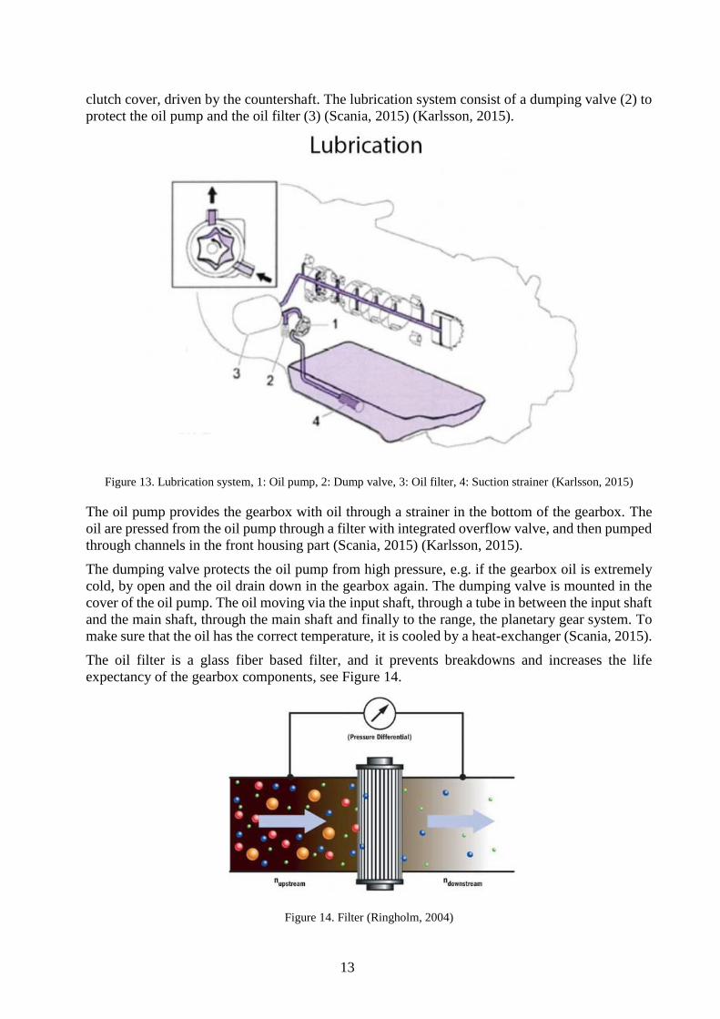
components (Scania, 2015). The oil pump (1) in Figure 13 is a rotor pump that is mounted in the

13

clutch cover, driven by the countershaft. The lubrication system consist of a dumping valve (2) to

protect the oil pump and the oil filter (3) (Scania, 2015) (Karlsson, 2015).

Figure 13. Lubrication system, 1: Oil pump, 2: Dump valve, 3: Oil filter, 4: Suction strainer (Karlsson, 2015)

The oil pump provides the gearbox with oil through a strainer in the bottom of the gearbox. The

oil are pressed from the oil pump through a filter with integrated overflow valve, and then pumped

through channels in the front housing part (Scania, 2015) (Karlsson, 2015).

The dumping valve protects the oil pump from high pressure, e.g. if the gearbox oil is extremely

cold, by open and the oil drain down in the gearbox again. The dumping valve is mounted in the

cover of the oil pump. The oil moving via the input shaft, through a tube in between the input shaft

and the main shaft, through the main shaft and finally to the range, the planetary gear system. To

make sure that the oil has the correct temperature, it is cooled by a heat-exchanger (Scania, 2015).

The oil filter is a glass fiber based filter, and it prevents breakdowns and increases the life

expectancy of the gearbox components, see Figure 14.

Figure 14. Filter (Ringholm, 2004)

14

Figure 15 illustrate the filter middle part that connect the gearbox, filter and heat-exchanger. The

oil flow from the gearbox, to the filter, to the heat-exchanger and then back to the gearbox again.

Figure 15. Oil filter middle part, Red line: Oil (out), Green line: Oil (in)

There is not a lot of wear particle when endurance testing the gearbox and the amount of oil passing

through the filter is high. For the amount of wear particle after an endurance test of a flawless

gearbox, see Figure 16.

Figure 16. The amount of metal particle in the gearbox after an endurance test

As seen in Figure 16, the amount of particles is larger for the first 32 million revolutions and it

depends on the running-in effect of the gearbox. If a component is defected in the gearbox, the

wear particles will increase. Therefore the amount of wear particles in the lubricant can be used as

indicator to identify defected components.

15

2.1.6 Gearbox faults

Gears, bearings and shafts are the main components in a gearbox. The main purpose of the gear is

to change the speed of rotation, the bearing supports the rotating shafts and the shafts are

transmitting the torque (phmsociety, 2009). The main purpose of the gearbox is to transfer the

power from the engine to the wheels, which means that the forces will be transferred between the

shafts. The best possible condition would be if all the components are perfectly balanced during

power transmission, which is not the case. The main reasons for shortening of the gearbox life are

unbalance, misalignment and/or poor lubrication, which lead to bearing failures, gear

misalignment and particles in the lubrication (Mohanty, 2015, pp. 94-112).

UNBALANCE

There are two different types of unbalance in the gearbox: static and dynamic unbalance. Static

unbalance occur when the center of mass is not coincident with the center of rotation and dynamic

unbalance, e.g. when a component is welded to a plate with an angle. The result of the

consequences of unbalance will vary, because it depends on the cause, position, type of unbalance,

etc. (Mohanty, 2015, pp. 98-100) (Lindholm, 1995, pp. 14-20).

MISALIGNMENT

Misalignment is caused by two shafts that are displaced in relation to each other, which can cause

faults in the gears, bearings, seals, etc. Another result of misalignment is bending of the shafts and

fatigue, leakage of the lubrication, heating, energy loss, etc. The misalignment occurs manly by

poor assembly work, changing of temperatures, load changes, changes of the rotational speed and

also outer forces. There are three different types of misalignment: internal misalignment, offset

misalignment and angular misalignment, see Figure 17 (Mobley, 2001, p. 797) (Lindholm, 1995,

pp. 21-27).

Figure 17. Different types of misalignments (Mobley, 2001, p. 797)

GEARS

The profile of the gear is designed to give a constant output speed for a constant input speed. A

common gear profile is an involute profile, because with this profile the speed ratio become less

sensitive to small variations of the center distance, even if the pressure angle, see Figure 18,

changes. In real life, the situation is not ideal for gears because of teeth deformation under loading.

The deformation leads to a meshing error or transmission error (TE), because of geometric

deviations. The deviations can both be intentional and unintentional. The intentional deviations

16

can e.g. be “tip relief”, where metal removed from the tip of each tooth. This makes it easier for

the teeth to come into mesh, without any kind of impact. While unintentional can lead to surface

fatigue failure or even gear-tooth fatigue (Randall, 2010, pp. 40-41).

Figure 18. Spur Gear - Pressure angle (Randall, 2010, p. 41)

Gear tooth failure

Failure of the gear tooth is generally a result from a crack originating in the root section of the

tooth. The strength of the material for gear-tooth failure can be affected by the surface finish, the

level of silicon, the shot peening or/and the hardening (Shipley, 1967) (Olsson, 1997).

Surface fatigue failure

There are different types of surface fatigue failure, and some of these are described below (Shipley,

1967).

Pitting – There are two types of pitting: initial pitting and destructive pitting. Initial pitting

is characterized by small pits on the surface. While destructive pitting is larger than initial

pitting.

Spalling – Spalling is similar to destructive pitting, the difference is that the pits are usually

larger in diameter. The area of spalling does not usually has a uniform diameter.

Scoring – There is different types of scoring: moderate scoring and destructive scoring.

Moderate Scoring show a characteristic wear pattern. While destructive scoring shows

definite indications of radial scratch in the sliding direction.

Abrasive wear – Abrasive wear occur when contact between surfaces has led to scratch

marks or grooves on the surface.

Corrosive wear – This failure is caused by a chemical action. It is often because of

ingredients from the lubricating oil.

The result of surface fatigue failure is not as dramatic as a gear tooth failure, but the level of

vibrations and the losses of the effect can lead to shortening of the life of the gear. The strength of

the material for surface fatigue failure and the life length can be affected by a lot of different

factors. The material should be homogeny and no micro defects approximately 0.5 mm from the

surface. The lubrication is important because it affects the gear life length. The oil thickness is

only about 2-3 µm where the highest pressure is, and even a particle of only 10 µm can increase

the tension. The temperature of the oil can affect the properties of the lubrication (Olsson, 1997).

17

BEARINGS

The damage of bearings is caused by the forces that is passing the bearings from the inside of the

gearbox and out, or the surrounding forces. This can be a result from by e.g. unbalance,

misalignment, bent shafts, defects, poor lubrication etc. The failures of the bearings are:

Wear – Result of poor lubrication. There are different types of wear, such as pitting,

flaking, scoring, etc. (SKF, 1994).

Corrosion – Chemical attack to the metal of the bearing. Corrosion can cover both a large

and a small area and it is often a result of oxidation (Torrington, 2000).

Misalignment – A misaligned bearing can lead to a lot of damage and it will probably lead

to breakage (Torrington, 2000).

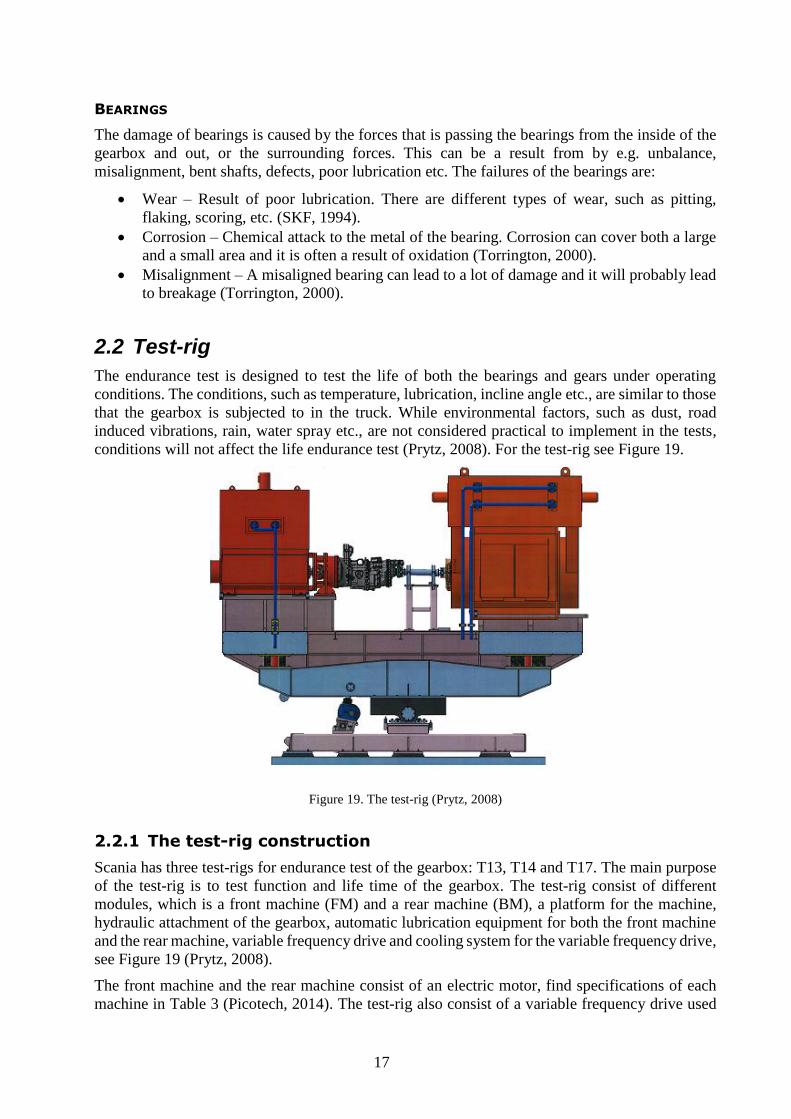
2.2 Test-rig

The endurance test is designed to test the life of both the bearings and gears under operating

conditions. The conditions, such as temperature, lubrication, incline angle etc., are similar to those

that the gearbox is subjected to in the truck. While environmental factors, such as dust, road

induced vibrations, rain, water spray etc., are not considered practical to implement in the tests,

conditions will not affect the life endurance test (Prytz, 2008). For the test-rig see Figure 19.

Figure 19. The test-rig (Prytz, 2008)

2.2.1 The test-rig construction

Scania has three test-rigs for endurance test of the gearbox: T13, T14 and T17. The main purpose

of the test-rig is to test function and life time of the gearbox. The test-rig consist of different

modules, which is a front machine (FM) and a rear machine (BM), a platform for the machine,

hydraulic attachment of the gearbox, automatic lubrication equipment for both the front machine

and the rear machine, variable frequency drive and cooling system for the variable frequency drive,

see Figure 19 (Prytz, 2008).

The front machine and the rear machine consist of an electric motor, find specifications of each

machine in Table 3 (Picotech, 2014). The test-rig also consist of a variable frequency drive used

18

for controlling the speed of the motors, instead of using the motor at a fixed speed. The variable

frequency drive consist of an ASi-system with emergency stop functions (Prytz, 2008).

Table 3. Specifications of the front machine and the rear machine (Prytz, 2008)

Specifications of the machines

The front machine The rear machine

900 kW 1900 kW

6500 Nm form 0 – 1320 rpm 27 000 Nm from 0 – 700 rpm

1320 rpm at continuous drive 700 rpm at continuous drive

3400 Nm at 2500 rpm 3100 Nm at 3200 rpm

Weight = 6 ton Weight = 12 ton

The gears are shifted automatically during the test by an OptiCruise-technique (OPC), which is an

automatic gear shifting system for manual gearboxes, and a transmission control unit (TCU),

which is an electronic OPC-control unit for the gearbox. During the shifting CAN (Control Area

Network), which is serial communication protocols between different control units, sends

messages between the control systems. When the gears are shifted, the gearbox stops and after the

gear shifting procedure it continues. The operator do not have to be present during the gear shifting

(Einarsson, 2011). Figure 20 show a gearbox that is mounted in one of the test-rigs called T17.

Figure 20. Test-rig: T17

19

2.2.2 Tilting device

The tilting device, see Figure 19, consist of two parts: a bottom part and a tilting plate. The bottom

part is mounted on the base frame of the rig. Bearing houses enable mounting of the tilting plate.

The tilting plate consists of electric motors mounted 1000 mm over the ground level. The changing

of the angle is accomplished by an electric driven spindle. The outer level is +/- 9° measured from

the reference angle, which is 5°. The spindles are equipped with a safety nut and the rotation of

the spindle is controlled. The electric motor driving the spindles is equipped with an electric brake.

The tilting device also consist of a caption ring, that is protecting the device if e.g. the cardan shaft

would break (Prytz, 2008).

2.2.3 Clamping device

The clamping device of the test-rig consists of twelve hydraulic cylinders, see Figure 21. The

construction is adaptable on the gearbox with a height of the flange of 35 mm. A ring with cylinders

is mounted on the front electric motor. It is possible to disassemble the ring by disconnecting the

screws. There are different types of rings, depending on the gearbox. Every cylinder consists of a

sensor, which indicates the correct clamping. The correct position of the gearbox is controlled by

a laser sensor. If the sensor detects any kind of movement of the gearbox, then the test will be

stopped. The hydraulic system consists of a redundant pressure sensor, which is connected to the

Scania ASi-system, a safety system. The clamping of the gearboxes is only possible if the base

frame of the test-rig is horizontal (Prytz, 2008).

Figure 21. Clamping device (Prytz, 2008)

2.2.4 Oil system

The oil system provide the gearbox with oil, and the main component of the system is the

filling/draining system, which is an “oil bar”. The oil, 75W90 GL5, is manually refilled by the

operator, and the wasted oil is collected in a stainless steel plate under the gearbox. The wasted oil

can be sucked up from the stainless steel plate by using a suction hose from an oil bar. A level

sensor mounted on the steel plate indicates when 1 litre of the oil has been collected, and if so the

test will be stopped (Gustavsson, 2006).

During the endurance test it is important that the oil has a temperature of about 100 C. Therefore

the oil temperature in and out are measured by sensors. For the temperature sensors that measuring

the temperature out of the gearbox see component 3 Figure 23. To measure the oil pressure during

the endurance test a pressure sensor is used. It is important that the pressure of the oil is 2.3 bar –

2.8 bar (Gustavsson, 2006).

20

In Figure 23 the oil level sensor is connected to an electrical connector (4) and if needed there is

also a connection for a temperature sensor (5) (Gustavsson, 2006). For a schematic illustration of

the oil system see Figure 22.

Figure 22. A schematic illustration of the oil system: 1: Heat-exchanger, 2: Quick connection, 3: Temperature

sensor, 4: Temperature sensor, 5: Pressure sensor, 6: Quick connection, 7: Level sensor. (Gustavsson, 2006)

Figure 23. Oil system: 1: Quick connection, 2: Oil plug, 3: Oil temperature sensor (TV01), 4: Oil level sensor, 5:

Temperature sensor, Pump for waste oil: 6: Valve 1, 7: Valve 2, 8: Valve 3. (Gustavsson, 2006)

21

2.3 Weibull analysis

Weibull analysis, also called “In life data analysis”, is widely used in reliability engineering. The

purpose of the Weibull analysis is to make predictions about the life of a product by fitting a

statistical distribution to life data from a representative sample of units. The statistical distribution

can be used for estimation of e.g. reliability or probability of failure at a specified time, the mean

life and failure rate. The requirements for a Weibull analysis are described below (Weibull, 2015).

Gathered life data for the product.

Selection of a lifetime distribution that fit the data and also model the life of the product.

Estimation of the parameters that will fit the distribution to the data.

Generation of plots and results. These will estimate the life characteristics of the product,

e.g. the reliability or mean life.

The Weibull analysis provides a simple graphical solution, where the horizontal scale is the life

length scale, e.g. the operating time or start/stop cycles, and the vertical scale is the probability of

failure, see Figure 24 (Abernethy, et al., 1983, pp. 1-2).

Figure 24. The Weibull analysis process (Abernethy, et al., 1983, p. 3)

The slope of the Weibull distribution can describe more than the probability of failure, it can also

provide an idea of the source of failure, such as corrosion or the bearings. In Figure 25 the

relationship between the failure modes and values of the slope are presented. In these cases the

slope of the line is called Beta (β) (Abernethy, et al., 1983, p. 2).

Figure 25. Description of the result (Abernethy, et al., 1983, p. 4)

22

Beta (β) determines which member of the family of Weibull distribution is the best description of

the data. A value of β < 1 indicates that the failure rate decreases over time, if β = 1, this indicates

that the failure rate is constant over time and a value of β > 1 indicates that the failure rate increase

with time. Sometimes it is of interest to determine the time which 1 % of the gearbox will fail or

determining the time at which one tenth of 1 % of the gearboxes will fail. Both these values can

be read from the curve. If a failure would occur in service operations, it is interesting to predict the

number of failures that might occur over the next four weeks, three month, six month etc. For an

example of a Weibull risk forecast, see Table 4 (Abernethy, et al., 1983, pp. 2-5).

Table 4. Weibull Risk Forecast (Abernethy, et al., 1983, p. 7)

Risk Prediction for 6 month

11.77 0.00 More failures in 0 month







As long as the endurance life of a component is known, for both the broken and working ones, it

is possible to calculate the failure probability for every life length of the breakage and draw these

in a Weibull diagram. A Weibull distribution function is then suited for the outcome (Abernethy,

et al., 1983, pp. 2-7). The test life data collected from the chosen condition monitoring system

should be suitable for a Weibull analysis, to predict L50 with a higher degree of statistical

confidence.

2.4 Condition Monitoring (CM)

The majority of the machines presented in the industry today have rotating components. The

machines should perform as their system specifications and their capacity. To ensure their

performance the machine must be in proper condition. Condition monitoring (CM) is a process

where the condition of the machinery is determined and analyzed during operation (Mohanty,

2015, pp. 1-4). The process has been divided into three phases: detection, diagnosis and prognosis

of faults in the machinery, see Figure 26. First, abnormal condition is detected, e.g. by a sensor,

then the signal from the sensor is translated into information and finally the information is analyzed

and forecasted (Randall, 2010, pp. 143-165).

Figure 26. The condition monitoring process

23

It is important to know the baseline (normal) condition and the trend of a specific part to determine

the condition of the machinery. When the behavior of a part is known and how its behavior change

over time it is possible to determine when the performance of the machinery has reached an

alarming level. Trending is the behavior of the machinery, from baseline condition until the

machinery is turned off. The condition is monitored in five steps (Forsthoffer, 2011, p. 553):

Definition of each component

List condition monitoring parameters

Obtaining of baseline data

Obtaining trend data

Establishment of threshold limits.

Transducers can be installed to measure signals from the gearbox, such as vibration, noise,

temperature, lubricating oil condition etc. The signals are converted by analog/digital converters

and then analyzed by computers. The data can then be used in algorithms to detect faults. Measures

can be adjusted after fault detection via this data. The advantages with using condition monitoring

processes are stated below (Mohanty, 2015, pp. 1-4).

Elimination of unnecessary maintenance

Reduction of rework costs

Reduction of repair parts inventory

Increase the efficiency of the process

Improve the quality of the product

Increase overall profit

Transducers, instrumentation, signal analysis software and a decision-making system are the most

important aspects when condition monitoring a machine, and these are continually being

developed. The most common system is vibration monitoring. The vibrations are often measured

by contact piezoelectric accelerometers, or laser-based systems for noncontact. The advantage of

the laser-based systems is that they can measure both transverse and rotational vibration of a

rotating machine. Wear debris monitoring and oil analysis are often performed in dedicated third-

party laboratories. Motor current signature analysis is mostly used to determine faults in an

electrical motor driving machine (Mohanty, 2015, pp. 2-3).

Many non-destructive methods (NDT) have become available for determination of internal defects

in machine components, and about 10 % of the condition monitoring methods is NDT methods

(Mohanty, 2015, p. 157). The most common non-destructive method is ultrasonic testing, where a

three-dimensional view of the inside of a part is collected. This is obtained by a surface scan, which

is quick. The second most common method is infrared thermal imaging, which detect defects by

analyzing the temperature (Mohanty, 2015, pp. 2-3).

2.5 Vibration

Vibration monitoring is the most common condition monitoring system used today, and it is

probably because of its diversity. This system is applicable to both nonlinearly and linearly moving

equipment. Vibration monitoring can be used for controlling the quality, detect cracks and to

analyze the flow of a fluid. It is important to be able to separate the characteristic vibration from

the uncharacteristic to analyze the result from the vibrations measuring. A shaft e.g. is supposed

to rotate, while some faults, such as loose gears, misalignment of shafts, worn bearings, etc. this

result in a typical vibration and it is important to be able to distinguish these vibrations (Mohanty,

2015, p. 93).

24

2.5.1 Fundamentals of machinery vibration

The motion of a body is represented by a vibration and it is essentially oscillatory about a mean

position of the body. The vibration can be periodic or aperiodic can be described in all the different

directions. The degree of freedom is the number of independent coordinates and it is used to

describe the motion of a rigid body, e.g. a rigid body in space has 6 degrees of freedom and the

rigid body consist of three translator motions and also three rotational motions about the axes

(Mohanty, 2015, p. 13).

A body of mass (m) is supported with a linear spring stiffness k, see Figure 27 (Mohanty, 2015, p.

13).

Figure 27. Single degree-of-freedom (Undamped system) (Mohanty, 2015, p. 14)

It is only possible for the body in Figure 27 to have motion in one direction, and the formula for

the motion of the body is given in Equation (1), a linear differential equation of the first order

(Mohanty, 2015, p. 13).

𝑚

𝑑2𝑥

𝑑𝑡2+ 𝑘𝑥 = 0

(1)

A solution to Equation (1) is the response 𝑋(𝑡) of the form 𝑥(𝑡) = 𝑋𝑒𝑖𝜔𝑡. With initial conditions

the constant called X can be found, such a response of the body is called the undamped free

vibration response of an oscillator that is harmonic. The frequency of this kind of systems is 𝜔𝑛 =

√𝑘 𝑚⁄ . In real life there is no undamped system, therefore a damped oscillator is illustrated in

Figure 28. Both Figure 27 and Figure 28 illustrate a scenario where the body is not subjected to

any external force or torque (Mohanty, 2015, p. 14).

Figure 28. Single degree-of freedom (Damped system) (Mohanty, 2015, p. 14)

25

The formula of a damped system with a single degree-of freedom is given in equation (2)

(Mohanty, 2015, p. 14).

𝑚

𝑑2𝑥

𝑑𝑡2+ 𝑐

𝑑𝑥

𝑑𝑡+ 𝑘𝑥 = 0

(2)

The coefficient of damping is C, which is known as viscous damping, which means that the

damping force is proportional to the body velocity. The factor of damping is given as 𝜁 =

𝐶 2√𝑘𝑚⁄ . The response of this kind of damped oscillator is given in Equation (3) (Mohanty, 2015,

p. 14).

𝑥(𝑡) = 𝐴−𝜁𝜔𝑡sin (𝜔𝑑𝑡 + 𝜙) (3)

where, 𝜔𝑑 = 𝜔𝑛√1 − 𝜁2

Figure 27 and Figure 28 represent a linear motion, but similar systems can also represent

oscillatory motions in rotation, as in a gearbox. Oscillatory motion in rotation is known as torsional

vibrations. The formula for the motion representing the free vibration response of a single degree-

of-freedom with damped torsional vibration is given in Equation (4) (Mohanty, 2015, p. 15).

𝐼

𝑑2𝜃

𝑑𝑡2+ 𝐶𝑡

𝑑𝜃

𝑑𝑡+ 𝑘𝑡𝜃 = 0

(4)

where,

𝐼 = The rotary mass moment of inertia

𝐶𝑡 = The torsional viscous damping coefficient

𝑘𝑡 = The torsional stiffness given in N-m/rad

θ = The rotational displacement

𝑑𝜃

𝑑𝑡= The rotational velocity

𝑑2𝜃

𝑑𝑡2 = The rotational velocity

To describe the motion and the vibrations in gearboxes the equations of motion are used. In rotating

machines, such as gearboxes, there are many different forms of excitation, such as forces as

couplings due to misalignment of the shaft, dynamic forces at the location of the bearings because

of movement of loose components, etc. Equation (5) describes the motion of a damped single

degree-of-freedom system that is subjected to an external force (Mohanty, 2015, p. 15).

𝑚

𝑑2𝑥

𝑑𝑡2+ 𝑐

𝑑𝑥

𝑑𝑡+ 𝑘𝑥 = 𝐹(𝑡)

(5)

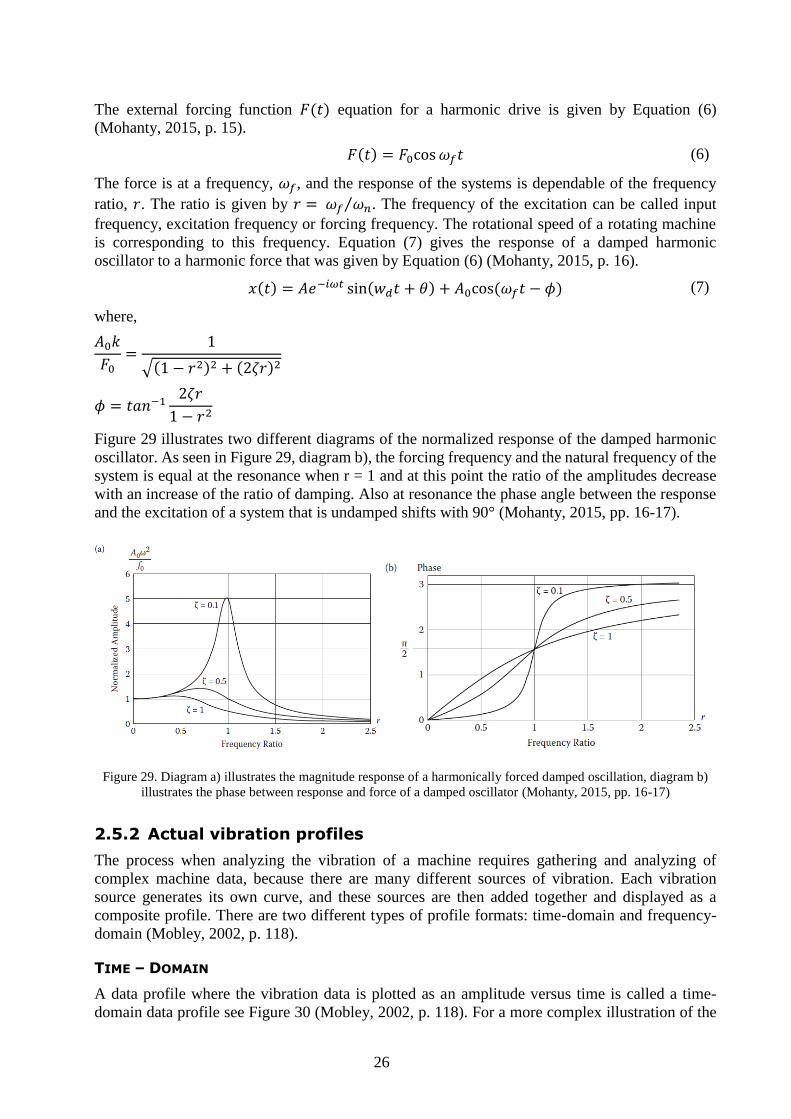
26

The external forcing function 𝐹(𝑡) equation for a harmonic drive is given by Equation (6)

(Mohanty, 2015, p. 15).

𝐹(𝑡) = 𝐹0cos 𝜔𝑓𝑡 (6)

The force is at a frequency, 𝜔𝑓, and the response of the systems is dependable of the frequency

ratio, 𝑟. The ratio is given by 𝑟 = 𝜔𝑓 𝜔𝑛⁄ . The frequency of the excitation can be called input

frequency, excitation frequency or forcing frequency. The rotational speed of a rotating machine

is corresponding to this frequency. Equation (7) gives the response of a damped harmonic

oscillator to a harmonic force that was given by Equation (6) (Mohanty, 2015, p. 16).

𝑥(𝑡) = 𝐴𝑒−𝑖𝜔𝑡 sin(𝑤𝑑𝑡 + 𝜃) + 𝐴0cos (𝜔𝑓𝑡 − 𝜙) (7)

where,

𝐴0𝑘

𝐹0=

1

√(1 − 𝑟2)2 + (2𝜁𝑟)2

𝜙 = 𝑡𝑎𝑛−12𝜁𝑟

1 − 𝑟2

Figure 29 illustrates two different diagrams of the normalized response of the damped harmonic

oscillator. As seen in Figure 29, diagram b), the forcing frequency and the natural frequency of the

system is equal at the resonance when r = 1 and at this point the ratio of the amplitudes decrease

with an increase of the ratio of damping. Also at resonance the phase angle between the response

and the excitation of a system that is undamped shifts with 90° (Mohanty, 2015, pp. 16-17).

Figure 29. Diagram a) illustrates the magnitude response of a harmonically forced damped oscillation, diagram b)

illustrates the phase between response and force of a damped oscillator (Mohanty, 2015, pp. 16-17)

2.5.2 Actual vibration profiles

The process when analyzing the vibration of a machine requires gathering and analyzing of

complex machine data, because there are many different sources of vibration. Each vibration

source generates its own curve, and these sources are then added together and displayed as a

composite profile. There are two different types of profile formats: time-domain and frequency-

domain (Mobley, 2002, p. 118).

TIME – DOMAIN

A data profile where the vibration data is plotted as an amplitude versus time is called a time-

domain data profile see Figure 30 (Mobley, 2002, p. 118). For a more complex illustration of the

27

time-domain for a piece of machinery see Figure 31, where the displacement is describe in mils

and 1 mil = 0.0254 mm (Newport, 2015).

Figure 30. Simple theoretical vibration curve (Mobley, 2002, p. 117)

Figure 31. An example of a time-domain vibration profile (Mobley, 2002, p. 119)

FREQUENCY - DOMAIN

The first step when analyzing the operating condition of a machine is to determine the circular

frequencies. The simple harmonic vibration functions are related to the circular frequencies of

rotating or moving components in a machine. The frequencies are expressed in revolutions per

minute (rpm) or sometimes cycles per minute (cpm). Frequency-domain data is obtained when

converting time-domain data (Mobley, 2002, pp. 119-120). Figure 32 illustrate an example of a

28

frequency-domain vibration profile, and the relationship between time-domain and frequency-

domain is illustrated in Figure 33.

Figure 32. An example of a frequency-domain vibration profile (Mobley, 2002, p. 120)

Figure 33. The relationship between the time-domain and the frequency-domain (Mobley, 2002, p. 150)

There are a lot of different mathematical techniques for converting time-domain data, such as Fast

Fourier transform (FFT), Hilbert-Huang transform (HHT), Teager-Huang transform (THT), Short

Time Fourier Transform (STFT), Wigner-Ville Distribution (WVD), Wavelet Transform (WT)

and Multiwavelet Transform.

Fast Fourier Transform (FFT)

The main problem addressed by the Fourier analysis is the analyzing of a function 𝑓 or

decomposing it into elementary components, which means that coefficients of 𝑓 are computed by

29

the mean of the inner product (𝑓, 𝑒𝑖𝑛𝑥) and to recover the function 𝑓, the products of the

coefficients are multiplied by the exponentials 𝑒𝑖𝑛𝑥 (Grünbaum, 1992).

One way used to convert time-based spectra to frequency-based is called Fast Fourier Transform

(FFT). The traditional analysis of the vibration signal relies upon the spectrum analysis via the

Fourier Transform, and it is a tool used to connect the time domain with the frequency domain

(Al-Badour, et al., 2011). The Fast Fourier Transform (FFT) accelerated the computation speed of

the transform in the 1960s (Mastro, 2013, p. 397). A signal 𝑓(𝑡) is transformed from a time-based

domain to a frequency-based one, by using the Fourier analysis, and generating the spectrum F(ω).

This spectrum includes all the signal’s constituent frequencies, see Equation (8) (Al-Badour, et al.,

2011). A disadvantage with the FFT is that it cannot provide any information about the time

dependence of the signal analyzed spectrum, and this become a problem for non-stationary signals.

𝐹(𝜔) = ∫ 𝑓(𝑡)𝑒−𝑖𝜔𝑡𝑑𝑡

∞

−∞

(8)

Hilbert-Huang Transform (HHT)

Hilbert-Huang transform is an empirically based data analysis method, and this kind of method

can produce a representation of data from a nonlinear and non-stationary process. The method

decomposes a signal into intrinsic mode functions (IMF), which lead to obtaining of instantaneous

frequency data. This method is similar to Fourier transform, but the IMF method is more like an

algorithm, an empirical approach, instead of a theoretical method. The result of the HHT is the

empirical mode decomposition (EMD). The HHT consist of two parts, which is Empirical Mode

Decomposition (EMD) and Hilbert Spectral Analysis (HSA). With this method it is possible to

deal with both non-stationary and non-linearity signals, and especially for time-frequency

representations (Shen & Huang, 2005, pp. 1-6). According to Huang et al. (1998) the intrinsic

mode function (IMF) is a function that satisfies the following two conditions.

1) In the whole data set, the number of extrema and the number of zero crossings must either

equal or differ at most by one.

2) At any point, the mean value of the envelope defined by the local maxima and the envelope

defined by the local minima is zero.

Condition one is equal to a traditional narrow band requirements for a stationary Gaussian process,

which mean that every point in some input space is associated with a normal distributed random

variable (Rasmussen & Williams, 2006). While the second condition make a modification of the

classical global requirement to a local one. All of the data are not IMFs and the collected data

involves more than one oscillatory mode, which means that Hilbert transform cannot provide full

description of the content of the frequency for general data (Huang, et al., 1998).

According to Huang et al. the empirical mode decomposition is based on the following three

assumptions.

1) The signal has at least two extrema, one minimum and one maximum.

2) The characteristic time scale is defined by the time lapse between the extrema

3) If the data were totally devoid of extrema but contained only inflection points, then it can

be differentiated once or more times to reveal the extrema. Final results can be obtained by

integration of the components.

30

Teager-Huang transform (THT)

The EMD is combined with a nonlinear operator called Teager Kaiser Energy Operator (TKEO)

to estimate the instantaneous frequency and also the instantaneous amplitude, and the name of the

association of the EMD and the TKEO is Teager-Huang transform (THT) (Li, et al., 2010).

Short Time Fourier Transform (STFT)

The limitations of the FFT have led to new methods, such as Short Time Fourier Transform

(STFT). With the STFT method a signal is mapped into a two-dimensional, 2D, function of time

and frequency. The method handle both non-stationary and non-linearity signals (Ai & Hui Li,

2009).

The disadvantage of this method is the limitation between the time and frequency resolution. It is

also difficult to use this method, because of the accuracy of extracting frequency information is

limited by the window length relative to the signal duration. This becomes a problem because

when the window is defined, the area remains fixed and this means that it is not possible for the

time and frequency resolution to increase simultaneously.

Wigner-Ville Distribution (WVD)

The method both handle non-stationary and non-linearity signals (Ai & Hui Li, 2009). While the

Wigner-Ville Distribution’s energy concentration in the time frequency plane is good. WVD is a

basic time-frequency representation. The disadvantage of this method is that interference terms

appear in the same plane, and this often misleads the analysis of the signal (Al-Badour, et al.,

2011).

Wavelet Transform (WT)

Wavelet transform method works in time and frequency domains. The graphs generated by this

technique are three dimensional time-frequency graphs that illustrate the vibration of the gear. It

shows the evolution with time, of the frequency spectrum of a signal. The wavelet map of the

residual vibration signal show a better indication of a crack, than the map of actual signal (Singh,

et al., 1999).

The wavelet transform is a powerful tool in the field of signal processing, and this method can be

used when having non-stationary signals. With the WT method it is possible to use both long and

shorter time intervals. When using long intervals precise low-frequency information is desired,

while using shorter time intervals accurate high frequency information is desired. The extraction

of the narrow-band frequency signal is more accurate when using this method. The disadvantage

with the WT is the possibility to perform a local signal analysis. It is also possible to zoom on any

specific interval of time, without losing the information of the spectral. By using the WT method

it is possible to reveal hidden aspects of the data, which is impossible for other techniques. One

limitation with this method is that the resolution of the frequency can be poor in the high frequency

regions, but with this method it is possible to achieve high frequency resolution with sharper

resolution than for the STFT method (Li, et al., 2005). A wavelet ψ(t), which is a waveform of

effectively limited duration with an average value of zero, is showed in Equation (9) (Al-Badour,

et al., 2011). The advantage of the Wavelet Transform compared to the Fourier analysis is that it

is possible to locate the analysis of a signal in both time and frequency (Grünbaum, 1992).

∫ 𝜓(𝑡)𝑑𝑡 = 0

∞

−∞

(9)

31

Multiwavelet transform

The Multiwavelet method is used for analyzing the experimental signal. The wavelet transform

uses vector scaling functions and wavelet functions when diagnose the machine. The first

polynomial multiwavelet transform was introduced by Alpert, 1993 (Sun, et al., 2014). The

applications of the method are video and image processing, data compression, coding, fault

diagnosis, etc. The main problem solved by wavelet theory is analyzing of a function or

decomposing the function 𝑓 into elementary components, is similar to the Fourier analysis.

Physical phenomena, such as vibrating sting, has to be studied to decomposing a function into

harmonics, but it is quite similar to analyzing a signal 𝑓 that has no connection to vibrating strings

(Grünbaum, 1992).

According to Sun, et al. (2013) the Multiwavelet transforms has received more attention in both

theory and in application from the wavelet. The main goal of the method for diagnosis of

mechanical fault is searching for the optimal basis function that is most similar to the fault features

in a given signal. Jaffard et al. (2001) describe how to choose the most optimal basis functions:

“Each algorithm is presented in terms of a particular orthogonal basis. We can compare

searching for the optimal algorithm to searching for the best point of view, or best perspective, to

look at a statue in a museum. Each point of view reveals certain parts of the statue and obscures

others. We change our point of view to find the best one by going around the statue. In effect, we

make a rotation; we change the orthonormal basis of reference to find the optimal basis” - (Jaffard,

et al., 2001, p. 11)

2.5.3 Source of vibration

Theoretical, all the forces acting on machines are equilibrium, but not in real life and this cause

vibration, such as small differences between the input shaft and the output shaft. The peaks in the

frequency-domain plots are the signature vibrations. When the components in a gearbox is not

perfectly balanced, it leads to vibrations. The vibrations are caused by both unstable media flowing

through the machine and the rotation of elements, such as gears, bearings and shafts. The result of

unstable flow is, e.g. deflection for the rotating parts from their center-line. When there are any

deviations from the condition the gearbox is designed for, it can lead to unstable flow. The load

change vibration is bigger compared to the vibration profile of flow, but it still creates a peak in a

frequency-domain plot (Mohanty, 2015, pp. 94-112).

Failure in one gear tooth will lead to disturbance one time per revolution and if two gear teeth are

damaged this will result in disturbances twice per revolution and so on. The measurement of the

vibrations can be done on the gearbox housing, because it amplifies the noise. A damaged gear

tooth will result in a change in the level of vibrations, e.g. a crack in a gear tooth will lead to a

sudden change of the vibration and a decrease in the amplitude of the disturbance limit can be

noticed. Non damaged gear teeth will also result in vibrations at the number of gear teeth times the

speed of rotation. Therefore it is important to make a comparison between the resulted spectrum

of vibrations and the reference spectrum where the gear was new (Mohanty, 2015, pp. 94-112).

The damage of bearings can cause vibrations, which can be a result from unbalanced shafts,

misalignment, bent shaft, poor lubrication, etc. The vibrations from a gear tooth failure can also

cause faults in the bearings.

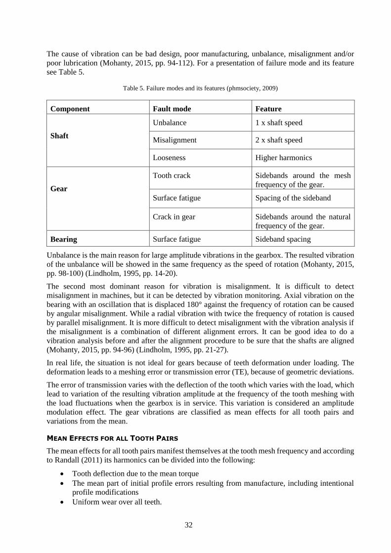
32

The cause of vibration can be bad design, poor manufacturing, unbalance, misalignment and/or

poor lubrication (Mohanty, 2015, pp. 94-112). For a presentation of failure mode and its feature

see Table 5.

Table 5. Failure modes and its features (phmsociety, 2009)

Component Fault mode Feature

Shaft

Unbalance 1 x shaft speed

Misalignment 2 x shaft speed

Looseness Higher harmonics

Gear

Tooth crack Sidebands around the mesh

frequency of the gear.

Surface fatigue Spacing of the sideband

Crack in gear Sidebands around the natural

frequency of the gear.

Bearing Surface fatigue Sideband spacing

Unbalance is the main reason for large amplitude vibrations in the gearbox. The resulted vibration

of the unbalance will be showed in the same frequency as the speed of rotation (Mohanty, 2015,

pp. 98-100) (Lindholm, 1995, pp. 14-20).

The second most dominant reason for vibration is misalignment. It is difficult to detect

misalignment in machines, but it can be detected by vibration monitoring. Axial vibration on the

bearing with an oscillation that is displaced 180° against the frequency of rotation can be caused

by angular misalignment. While a radial vibration with twice the frequency of rotation is caused

by parallel misalignment. It is more difficult to detect misalignment with the vibration analysis if

the misalignment is a combination of different alignment errors. It can be good idea to do a

vibration analysis before and after the alignment procedure to be sure that the shafts are aligned

(Mohanty, 2015, pp. 94-96) (Lindholm, 1995, pp. 21-27).

In real life, the situation is not ideal for gears because of teeth deformation under loading. The

deformation leads to a meshing error or transmission error (TE), because of geometric deviations.

The error of transmission varies with the deflection of the tooth which varies with the load, which

lead to variation of the resulting vibration amplitude at the frequency of the tooth meshing with

the load fluctuations when the gearbox is in service. This variation is considered an amplitude

modulation effect. The gear vibrations are classified as mean effects for all tooth pairs and

variations from the mean.

MEAN EFFECTS FOR ALL TOOTH PAIRS

The mean effects for all tooth pairs manifest themselves at the tooth mesh frequency and according

to Randall (2011) its harmonics can be divided into the following:

Tooth deflection due to the mean torque

The mean part of initial profile errors resulting from manufacture, including intentional

profile modifications

Uniform wear over all teeth.

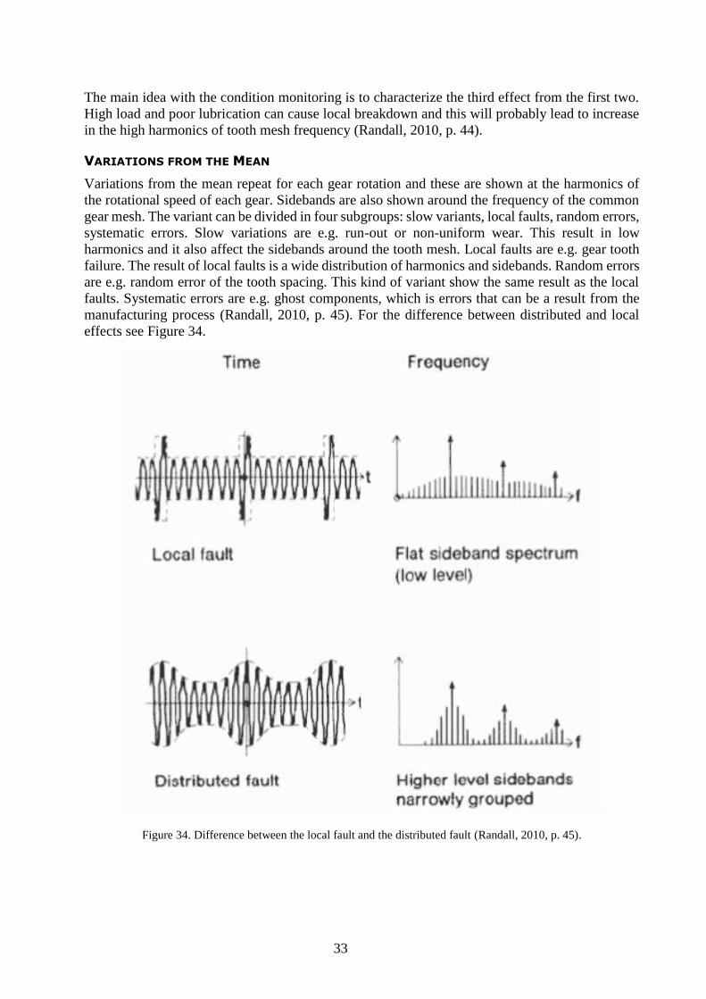
33

The main idea with the condition monitoring is to characterize the third effect from the first two.

High load and poor lubrication can cause local breakdown and this will probably lead to increase

in the high harmonics of tooth mesh frequency (Randall, 2010, p. 44).

VARIATIONS FROM THE MEAN

Variations from the mean repeat for each gear rotation and these are shown at the harmonics of

the rotational speed of each gear. Sidebands are also shown around the frequency of the common

gear mesh. The variant can be divided in four subgroups: slow variants, local faults, random errors,

systematic errors. Slow variations are e.g. run-out or non-uniform wear. This result in low

harmonics and it also affect the sidebands around the tooth mesh. Local faults are e.g. gear tooth

failure. The result of local faults is a wide distribution of harmonics and sidebands. Random errors

are e.g. random error of the tooth spacing. This kind of variant show the same result as the local

faults. Systematic errors are e.g. ghost components, which is errors that can be a result from the

manufacturing process (Randall, 2010, p. 45). For the difference between distributed and local

effects see Figure 34.

Figure 34. Difference between the local fault and the distributed fault (Randall, 2010, p. 45).

34

2.5.4 Detection of damages

To detect fault in the gearbox, it is important to be able to distinguish the vibration in the spectrum

of frequency caused by a damaged part from the normal vibration caused by an undamaged part,

which can be difficult. Therefore techniques has been developed to help with this problem and

also to distinguish vibrations from the background noise, which is scaling, filtering, envelop, SEE,

SPM and kurtosis (Mohanty, 2015, pp. 93-112).

SCALING

This is a scaling technique, which makes it possible to zoom the frequency of interest, by e.g. using

a log-scale. Access to the frequency of the bearings and drawing them as line in the spectrum of

frequency can make it easier to use the scaling technique.

FILTERING

It is important to distinguish a normal vibration from a vibration from a damaged component, and

this technique filtering out the frequencies from the normal vibration. This makes the frequencies

of interest more clear.

ENVELOPING

Enveloping is a computer based system. The base of the envelope detection method is the fact that

a crack in a tooth will result in an amplitude and phase modulation of the resulted vibration signal

when there is a damage in a tooth. This method has a sequential collection of data. The theory of

the enveloping method is to move the frequency band to be analyzed to higher frequencies, with a

maximum of 80 kHz, and then eliminate the normal frequencies (Singh, et al., 1999).

SEE

The method is similar to the Enveloping technique, but with the SEE it is possible to move the

frequency band to higher frequencies, with a maximum of 340 – 400 kHz. The SEE technique also

utilizes an acoustic transducer to measure the bearings.

THE SHOCK PULSE METHOD (SPM)

The shock pulse method (SPM) was developed in the 1969 and is mostly used to detect the short

duration shock waves that damages of rolling bearing cause, but it can also be used for identifying

loose parts, misalignment and also cavitation. This method utilizes a logarithmic scale to analyze

the resulted shock pulse from faults in bearings. PE sensors, similar to accelerometers but these

sensors are operated at their resonant frequency (32 kHz), are used for detection of the waves. This

means that even weak shock pulses can give large output signals. 32 kHz is chosen because it is a

compromise, which means that it is above the interfering low frequency signals from e.g.

unbalance or misalignment and it is below the ultrasonic frequencies. Otherwise the ultrasonic

frequencies can affect the signal. The vibration of components that have a lower frequency will

also be filtered out. The instruments used for the SPM method give both readings of the magnitude

of the shock peaks, the maximum dBm value, and the signal level between the peaks, the carpet

dBc value. These two values describe the condition of the bearing. A FFT analysis on the signals

can also result in information of the nature of the fault (Bogue, 2013).

35

KURTOSIS

The Kurtosis method is defined as the normalized fourth statistical moment of the vibration image

and Kurtosis is a dimensionless number. It is the dimensionless number that indicates the health

of the gear. If a gear is healthy, then it generates a reasonably uniform vibration pattern at the

frequency of the gear. It also generates a low kurtosis value. While a tooth that has a crack or if it

is damaged result in a signal that is modulated, where the kurtosis value is a measure of the

peakiness of the vibration signal (Singh, et al., 1999).

2.5.5 Identification of vibrations

When identifying the source of the vibration in the frequency-domain plot, the vibration frequency

of the parts must be known, and also the amount of periodic peaks. If a round wheel is unbalanced

then it will cause vibration peaks one time per revolution. If the wheel rotate with a speed of 1000

rpm and the vibrations are one time per revolution, then there will be 1000 cycle per minute and

this result in a frequency of approximately 1000/60 = 16.67 Hz. It makes it easier to determine the

cause of the vibration if the plot is transferred from the time-domain to the frequency-domain plot.

This results in an easier way of looking at the amplitudes for different frequencies. The peaks in

the frequency-domain plot are related to a certain fault in the component (Mohanty, 2015, pp. 93-

112).

It is possible to deduce defects if the spectrum is different compared to the standard. In some cases

a line appears in the frequency spectrum at 160 Hz, if a component with 160 oscillations per second

occurs in the signal of time. While if a component occurs with 16 oscillations per revolution in the

time signal, this lead to a line at 16. This means the 16th order. Therefor the spectrum of the

rotationally synchronous time signal is called the order spectrum. When analyzing a gear wheel

with 16 teeth, 16 “clicks” will be heard per revolution. This is heard when the teeth of the gear

wheel mesh with the paired gear wheel. It is the “clicks” that produce a line in the order spectrum

at the 16th order, see Figure 35 (Discom, 2012).

Figure 35. Frequency Spectrum and Order Spectrum for a Gear Wheel (Discom, 2012)

The most dominating noise source is when the teeth of gear and wheel engage. The basic

frequency, e.g. the 16th order if a gear wheel has 16 teeth, is found in the spectrum with multiples,

which in this case are 32nd, 48th, 64th order etc. The base order is called the “first harmonic” or

“H1” and the double base order is called “second harmonic” or “H2”. In a gear wheel spectrum

the harmonics is recognizable, which means that no general defaults can be set for harmonic

patterns. Therefore the circumstances of a test have to act as a guideline instead. Sidebands can

36

also appear as a result from testing the gearbox. If the sidebands are high, then this can refer to

eccentricity or ovality. Different characteristic noses and noise patterns can occur for each test,

which means that the aggregate has the same defect as a previous test even if the noise or the

pattern look the same. For some common defects and its spectrum see Figure 36 (Discom, 2012).

Figure 36. Common Defects of a Gear Wheel (Discom, 2012)

37

If the gear wheel is good then only the orders H1, H2, H3 etc. will be seen in the synchronous

rotor spectrum. If there are nick or similar this will mainly be expressed in the time signal and it

is Crest value that record this. For nick that are really bad a “crest” will be seen in all whole orders.

While if the surface is defected, e.g. ripples or circular pitch errors, this will be expressed by

additional spectral lines. If ovality and eccentricity occur this lead to a modification of the meshing

noise, which lead to increased sidebands near the meshing orders. Features called “Hats” are used

to find sidebands. These are used for spectral limit curves (Discom, 2012).

Using a computer software that consist of the vibration data, the rotational speed and other

component and machine properties it is possible for the software to determine alarming for the

vibrations levels in the components. The resulted spectra when measuring vibrations can be

analyzed by using the software to calculate frequencies of the damages in a specific component

and show them as lines in the spectra. This makes it easier to observe peaks of vibrations that is

coincident with the frequencies of the damage (Mohanty, 2015, pp. 93-112). Figure 37 show a

spectra of a damaged bearing.

Figure 37. FFT plot of a bearing with a first order damage frequency (Vibrationschool, 2015)

Large vibrations from a damaged bearing only occur occasionally during the development of a

damage, and the vibrations can also decrease in a final stage, when a rolling bearing may have

become a kind of sliding bearing instead. A damaged bearing is discovered through various kinds

of frequency analysis, usually based on the shock pulses or shock waves generated by the damage

(Lindholm, 1995, pp. 45-46). There can e.g. be one or more of the balls that have been damages,

the inner or outer race or even the cage can be damaged, see Figure 38.

Figure 38. Outer race damage (Ludeca, 2011)

38

The four different bearing fundamental frequencies are a function of the pitch diameter, ball

diameter and the relative speed between the raceways, which is shown in the equations below

(Lindholm, 1995, pp. 45-48) (Graney & Starry, 2011) (Felten, 2003) (Ganeriwala, 2010).

𝐵𝑎𝑙𝑙 𝑝𝑎𝑠𝑠𝑖𝑛𝑔 𝑓𝑟𝑒𝑞𝑢𝑒𝑛𝑐𝑦 𝑜𝑢𝑡𝑒𝑟 𝑟𝑎𝑐𝑒 𝐵𝑃𝐹𝑂 =

𝑧 ∗ 𝑛

2 ∗ 60(1 −

𝑑

𝐷𝑐𝑜𝑠 𝜙)

(10)

𝐵𝑎𝑙𝑙 𝑝𝑎𝑠𝑠𝑖𝑛𝑔 𝑓𝑟𝑒𝑞𝑢𝑒𝑛𝑐𝑦 𝑖𝑛𝑛𝑒𝑟 𝑟𝑎𝑐𝑒 𝐵𝑃𝐹𝐼 =

𝑧 ∗ 𝑛

2 ∗ 60(1 +

𝑑

𝐷𝑐𝑜𝑠 𝜙)

(11)

𝐵𝑎𝑙𝑙 𝑠𝑝𝑖𝑛 𝑓𝑟𝑒𝑞𝑢𝑒𝑛𝑐𝑦 𝐵𝑆𝐹 =

𝐷 ∗ 𝑛

2𝑑 ∗ 60(1 − (

𝑑

𝐷)

2

𝑐𝑜𝑠2 𝜙) (12)

𝐹𝑢𝑛𝑑𝑎𝑚𝑒𝑛𝑡𝑎𝑙 𝑡𝑟𝑎𝑖𝑛 𝑓𝑟𝑒𝑞𝑢𝑒𝑛𝑐𝑦 𝐹𝑇𝐹 = 1 ∗ 𝑛 (1 −

𝑑

𝐷 𝑐𝑜𝑠 𝜙)

(13)

Where:

D = pitch diameter

d = ball diameter

z = number of balls

= contact angle

(For a definition of the symbols see Figure 39.)

Figure 39. Bearing symbol definition (Lindholm, 1995, p. 47)

2.5.6 Data acquisition

The most important when using the vibration monitoring is to have data that is reliable, accurate

and repeatable. It is important to keep records of historical key parameters to be able to compare

the result from the vibration analysis to earlier testing results to identify changes. The point of

measurement has to be at exactly the same point for the measurement to be repeatable (Mobley,

2001, p. 49).

Transducers are used to measure the vibrations in real-time, and these can be mounted at the

locations of interest. The device converts one form of energy to another form of energy, usually

39

an electrical signal. The most common transducer is the accelerometer with piezoelectric films,

which converts the compressions into measurable electric signals, and to collect and store the data

a portable vibration analyzer can be used. The portable vibration analyzer can convert the data and

perform e.g. a FFT. The instrument can also be programmed to set alarms and display the collected

data, but the results can also be transferred to a computer, which consists of more refined functions

(Mobley, 2001, p. 49).

When using the portable vibration equipment the vibrations from test-object is measured from

three different directions: horizontal, vertical and axial. The equipment for the measurement is

then removed to transfer and analyze the collected data and information about the test-object.

Transducers with a vibration analyzer that is portable can be called a semi-online system. A semi-

online system is a system that is online and it consist of accelerometers that continuously transfer

data and information to a computer whit an analyzing software system (Mobley, 2001, pp. 49-50).

TRANSDUCERS

There are different kinds of transducers for measuring vibrations, the major ones are displacement

probes, velocity transducers and accelerometers (Mobley, 2001, pp. 49-50).

Displacement probes

Displacement probes, or eddy-current probes, measuring the actual movement, or displacement,

of a component relative to the probe. The data is normally recorded as peak-to-peak in mils, and

this value is the maximum deflection or displacement for the component from the true centreline.

This kind of device must be attached to a stationary structure to obtain accurate and also repeatable

data. For an illustration of the displacement probe, see Figure 40. The most accurate data for a

machine with a rotor weight that is lower compared to the casing is provided by permanently

attached probes. It is more accurate for a turbine or large compressors to have the probes mounted

at key measurement location. The most useful frequency interval for the probes is between 10-

1000 Hz (600-60 000 rpm). If a component has a frequency lower or higher than the interval it

will be distorted, because this frequency is not reliable to determine the condition of the machine.

According to Keith Mobley (2001), the limitation of this technique is the cost, one probe costs

about $1000 and for accurate measurement about 10 probes are needed for a gearbox (Mobley,

2001, pp. 50-51).

Figure 40. Displacement probe and the system of the signal condition (Mobley, 2001, p. 50)

40

Velocity transducers

A velocity transducer is an electromechanical sensor and the transducer is designed to monitor

casing, or relative the vibration. The different between a displacement probe and the velocity

transducer is that the velocity transducer measures the displacement rate and not the moving

distance. Velocity is often described as millimeters per second (mm/sec) peak or inches per second

(in/sec), which according to Keith Mobley (2001) is the best method to express the machine

vibration energy. Figure 41 illustrate a schematic diagram of how the velocity is picked up. The

effective frequency range for the velocity transducers is 10-1000 Hz. These transducers should not

be used if the frequency is below or above this limit. A disadvantage with the velocity transducers

is that they are sensitive to mechanical and thermal damage. Normal use can also cause a loss of

calibration, therefore it is required to use a recalibration program to prevent errors of the resulted

data, and these should be recalibrated after 6 months. Even if they are calibrated every 6 months,

the transducers can provide misrepresented data (Mobley, 2001, pp. 51-52).

Figure 41. Schematic Diagram of a measurement device for the velocity: 1. Pickup case, 2. Wire out, 3. Damper, 4.

Mass, 5. Spring, 6. Magnet. (Mobley, 2001, p. 52)

Piezoelectric Accelerometers

Acceleration is probably the best methods to determining the resulted force from the vibration of

a machinery. The accelerometer consists of piezoelectric crystals or films that convert the

mechanical energy into electrical signals, and the generated electrical output is proportional to the

applied acceleration, see Figure 42 for a schematic drawing of a piezoelectric accelerometer

(Mobley, 2002, p. 155).

Figure 42. A piezoelectric accelerometer (PCB, 2015)

The effective frequency interval for the general accelerometers is 1 – 10 000 Hz, and for an

ultrasonic accelerometers it is even up to 1 MHz. If the vibration data is above 1000 Hz for a

general accelerometer, this should be analyzed in acceleration. The advantage of the accelerometer

compared to the velocity transducers is that no calibration program is needed. However, an

accelerometer is sensitive to thermal damage, which means that if heat radiates into one of the

piezoelectric films it can be damaged or in worst case destroyed. This kind of problem is rare if a

temporary mounting technique is used, because of the short data acquisition time (Mobley, 2001,

pp. 52-53).

41

Cymbal Piezoelectric Composite transducer

The transducer consist of a piezoelectric ceramic disk between two “cymbal” shaped metal end

caps, see Figure 43 for a schematic drawing of the transducer. The cymbal piezoelectric composite

transducer is similar to the piezoelectric accelerometer. The difference between these devices is

that the cymbal transducer has a higher piezoelectric charge coefficient and also faster response

time, which improve the detection of damaged components (Denghua, et al., 2010) (Sun, et al.,

2006).

Figure 43. Cymbal piezoelectric composite transducer (Denghua, et al., 2010)

CHOOSING TRANSDUCERS

When determine the most appropriate vibration analysis system it is important to take the

transducer’s characteristics into account. None of the described transducers above is suitable for

every application. The factors influencing the choice of transducer are measuring range, sensitivity

range, resolution range, dynamic range, frequency response, environmental factors, mass loading

effect and the cost (Gatti, 2003, pp. 639-642).

Measuring range

The piezoelectric sensors are usually used when measuring high-level acceleration, while for

medium-level accelerations all different kinds of transducers described above can be used. The

medium-level accelerations are encountered in most vibrations measurements (Gatti, 2003, pp.

639-640).

Sensitivity, resolution and dynamic range

The sensitivity, resolution and the dynamic range have been grouped together, because they are

correlated. If the sensitivity is high it result in a large amplitude force a measured level, but it is

the resolution limit that set the minimum level that is detectable. The dynamic range is equal to

the range of input levels measurable by the transducer. Both the piezoelectric accelerometer and

the dynamic piezoelectric composite transducer have a wide dynamic range (Gatti, 2003, p. 640).

Frequency response

When the frequency is low, the sensors must have a significant sensitivity. It is possible for the

piezoelectric accelerometer to extend their frequency limit below 1 Hz (Gatti, 2003, p. 640).

Environmental factors

The environmental factors can e.g. be the temperature, sound and dust. The piezoelectric

accelerometers have a temperature range of from -269 to 750C. If the transducers will operating

in high magnetic fields, special transducers are needed (Gatti, 2003, p. 641).

42

Mass loading effect

If the effective mass of vibration is low, then mass loading can become a problem. Therefore light

weighted transducers have to be used in these cases. It is difficult to know the structural mass, but

it can be tested. The signal from the accelerometer at a specific point of the structure is compared

with the obtained signal from identical sensor that is positioned close to the first one. The

measurement will result in errors if there is a significant different between the two responses from

the sensors (Gatti, 2003, pp. 641-642).

Cost

The cost becomes an important factor if a large amount of transducers are needed. The low-cost

piezoelectric transducers is perfect for modal analysis of structures, while smart accelerometers

with an onboard memory have become more common, because it is possible to store calibrations

and also identify parameters in an electronic data sheet developed for transducers, called TEDS

(Gatti, 2003, p. 642).

TRANSDUCER MOUNTING TECHNIQUES

The placement of the transducers are of great importance to achieve accurate measuring results. It

is important to make sure that the transducers are mounted correctly so they do not move

independently, which can lead to misleading signals. A link between the gearbox housing and the

transducer is necessary to obtain accurate measuring data. There are different techniques for

mounting the transducers: permanent, quick disconnect or magnets. How the transducers are

mounted depends on the monitored vibrations (Mobley, 2002, pp. 157-158).

Permanent

The permanent mounting technique is a good method to ensure that the point of measurement, its

orientations and the compressive load are the same for each test. The transducer can e.g. be glued,

stud mounted or double stud mounted, see Figure 44 (Mobley, 2002, pp. 157-158).

Figure 44. Permanent transducer mounting (Mobley, 2002, p. 158).

Quick Disconnect

A quick-disconnect stud is permanently mounted at each measuring point, and by using a mating

sleeve built into the transducer the pieces are connected. The quick disconnect mounting technique

is less expensive than permanent mounting, and it can almost provide the same accuracy and

repeatability (Mobley, 2002, p. 158).

Magnets

The transducer can also be attached with a magnet. The disadvantage with the magnet mounting

technique is that the resonant frequency of the transducer/magnet can lead to distortion of the data.

43

The magnet can be attached anywhere on the magnetic area of the machine, and it is important

that the area is fully magnetic. When using magnets attachment it is difficult to ensure that the

location of the transducer is maintained with each measurement (Mobley, 2002, p. 158).

2.5.7 Vibration analysis techniques

There are different techniques for analyzing vibrations: trending, comparative analysis and

signature analysis (Mobley, 2002, pp. 161-165).

TRENDING

The most common analysis tool for vibration-monitoring programs is trending, and the programs

often rely on historical vibration-level amplitude trends. Trend data that are valid can show change

over time within the condition of the machine (Mobley, 2002, p. 161).

Broadband

The overall machine condition is analyzed by the broadband by measuring the vibrations. The base

of the broadband technique is the overall vibration or energy from a frequency interval, 0 – the

maximum frequency chosen by the user. The broadband analysis is used for long term trending of

the overall condition of the machine (Mobley, 2002, p. 161).

Narrowband

The broadband and the narrowband analysis have the same function, but the advantage of the

narrowband analysis is the possibility for the user to select a specific group of frequencies. The

frequency selection makes it easier to monitor, trend and alarm specific machine components, e.g.

a specific set of gears (Mobley, 2002, p. 162).

COMPARATIVE ANALYSIS

The purpose of the comparative analysis is to compare two or more data sets to detect changes in

the condition of the machinery. It is not possible to determine the dynamics of the system, instead

the analysis method is limited to the comparison of frequency-domain signature, which is

generated by the machinery. The data generated is used for baseline data (Mobley, 2002, p. 162).

SIGNATURE ANALYSIS

A machine has a unique signature and it can be broken down into peaks. Each peak is a

representation of a specific component in the machinery. For a full-signature spectra analysis a

tremendous amount of microprocessor memory is needed, which is impractical and costly. An

optimum system is a system that can optimize the trending, preform a failure analysis of the root-

cause and at the same time maintain minimum data management to keep the memory costs low. A

full-signature spectrum is only needed when identification of a damaged component demands

further examination (Mobley, 2002, p. 163).

2.5.8 Advantages and disadvantages

The advantages of the vibration monitoring technique is that it is applicable for both linearly and

nonlinearly moving equipment and it can be used for controlling the quality, detect cracks and to

analyze the flow of fluid. The main disadvantage is the background noise, which makes it difficult

to detect faults because the signal-to-noise ratio (SNR) of the fault signal is low when damage

firstly appears. There are filtering techniques available to remove the background noise, so it is

possible to detect a fault in an early stage and avoid catastrophic failure.

44

According to Randall (2010, p. 6) the vibration analysis is the most prevalent method for

machinery condition monitoring, because of its advantages compared to other techniques available

on the market. Randall describes that vibration immediately reacts to changes, and compared to

oil analysis it is more likely to point to the damaged component.

2.6 Thermography

The main idea of the thermography system is that objects that have a temperature above zero will

emit energy or radiation. Infrared radiation is a form of emitted energy and the emission of infrared

energy, e.g. temperature, is monitored by special instrument design to determine the operation

condition of the machinery, see Figure 45. The infrared emission is invisible without special

instrumentation. The system detects thermal anomalies, areas which are hotter or colder than they

should be. The components in a gearbox have an operating temperature limit which is suitable to

use as a baseline when detecting thermal changes and vibrations. With a stationary system it is

possible to follow the development of the temperature continuously, which means that it is possible

to early detect arising of failures. It is complicated to use the infrared methods to measure the

temperature, because of the possible detection of three sources of thermal energy: energy emitted

from the test-object, energy reflected from the test-object and the energy that the object transmits.

It is only the emitted energy that is important for condition monitoring of the object. While the

reflected and transmitted energy will lead to misrepresentation of the raw infrared data. Therefore

it has to be filtered out before the analyzing of the data. The emitted and reflected energy is decided

by the surface of the test-object. A non-emitting surface is called Blackbody, and has an emissivity

of 1.0, while a surface that reflects energy is called Graybody, with an emissivity less than 1.0

(Saeed, 2008) (Mobley, 2001, p. 872).

Figure 45. Thermography (Supervision, 2014)

When using a thermography, it is important to consider the atmosphere between the test-object

and the measuring instrument, because the test can be distorted by water vapour, dust and some

lighting. Extreme care is needed, because the atmosphere is changing. Special filter can be used to

avoid the effects of the atmospheric changes, but it is important to know the factors that can affect

the accuracy of the infrared data to be able to apply a correct filter. The detection of thermal

anomalies has a wide range of applications in different machines, such as gearboxes, motors,

electric generators. There are different kinds of infrared instrument, but the most common

instrument is infrared imaging (Mobley, 2001, p. 872) (Saeed, 2008).

2.6.1 Infrared imaging

Infrared imaging makes it possible to scan the infrared emissions of machines in a short time,

which is not possible for other infrared techniques. The function of the imaging system is almost

45

like a video camera and it is possible to see the thermal emission profile by looking through the

optics of the instrument. There are different types of sensors used for infrared imaging: Infrared

IR sensors with one pixel and high resolution IR-cameras with many pixels. The IR temperature

transmitter has a field of view of about 10 degrees, which is rather wide. The advantage with the

sensors is that they do not need to be in contact with the test-object, but the IR temperature

transmitter has to be mounted close to the test-object (Anjar, et al., 2011).

THE PROCESS OF INFRARED IMAGING

An infrared thermal imaging camera and an IR scan are used when scanning the test-object. The

scan process can be set by appropriate time intervals that are predefined. When the scan starts it

takes thermal images of the defined object to find out the thermal anomalies in the system. The

thermal anomalies is defined by comparing the taken images with the baseline images of the object.

If no deviation is found, then the rescanning will start after a time interval set by the user. If the

scan has found any abnormality, then it will continue to the next step, which is to investigate the

problem using IR thermal imaging software (Saeed, 2008).

An identification of the nature of the problem is the first step of the diagnosis. When the fault is

identified, the priority of the problem is defined. This is done by using the priority and alarm list

that is predefined by the maintenance planner. If the result shows that the problem is in sever and

inadequate condition an IR report is generated for the information about the problem, such as

temperature gradient details and thermal patterns for detail investigation and for necessary

corrective actions that have to be made. If the result shows that there is not high priority for the

problem, then it is added to waiting stack until the rescanning starts again. If abnormality of the

problem is found, but it cannot be identified, then it will be further investigated by using vibration

and ultrasonic testing for the object (Saeed, 2008). The process is illustrated in Figure 46.

Figure 46. The process of Infrared Scanning (Saeed, 2008)


The advantage of thermography is that the point-of-use infrared thermometers are inexpensive. An

infrared instrument cost less than $1000. The cost of a black and white scanner is about $8000,

while a microprocessor based and a full color scanner cost about $60 000. Another advantage is

that the test-object and the component do not have to be in contact (Mobley, 2001, pp. 872-873).

46

The main disadvantage with the method is the atmosphere between the tested component and the

measuring instrument, because there are gases that can absorb infrared radiation. Filters can be

used to minimize the effect from the atmosphere. Therefore it is important that the user of the

imaging system knows the atmospherically effect (Mobley, 2001, pp. 872-873). Water vapor,

particles and light can also distort infrared radiation. Another problem with this method is that the

components in the gearbox both emit and absorb the transmitted infrared energy. Only the emitted

energy is needed for determine the condition of the component, which mean that the other energy

has to be filtered out before analyzing. Different factors can affect the component’s infrared energy

emitting ability, e.g. surface conditions and coatings, but there are tables for the emissivity for

most materials (Mobley, 2002, pp. 172-173).

2.7 Oil analysis

During operation the moving components in the gearbox rub against each other, and the friction

between the parts lead to energy dissipated as heat. The surfaces are often heat treated to become

more resistant to wear, but it does not matter how wear resistant the components are, because with

time particles will be dislodged from the surface. The particles will be deposited in the lubricating

oil. The size, shape, composition and quantity of the wear particles in the lubricant can give

information about the condition of the component (Mohanty, 2015, p. 147). Particles in the

lubricant can lead to changes of physical and chemical properties of the lubricating oil (Mohanty,

2015, p. 147). The different types of wear particles are described in Figure 47.

Figure 47. Wear particles (Peng & T.B, 1999)

47

Compared to vibration or any other method, oil analysis can provide an early warning of

impending failure (Mohanty, 2015, p. 147). Figure 48 show an illustration of the relationship

between the particles and the condition of the component.

Figure 48. Relationship between the generated particles and the condition of the component (Bogue, 2013)

There are many different techniques used to monitor wear particles. All manner of proprietary

product has been developed by the manufacturers to measure the true condition of the oil. The

magnetic plug is the simplest device, and it is located in a lubrication system. The main purpose

of the device is to attract and retain particles of ferromagnetic wear. These particles are then

removed and analyzed on a regular basis. The wear debris can be investigated both visually and

microscopically. Fine particles often arising from normal wear and the larger particles often is an

indication of accelerated process of wear. The disadvantage with traditional wear debris analysis

techniques, where the oil is taken and sent to a lab, is that the analysis can take several weeks and

while it is analyzed the component may have already failed. Therefore, new real-time wear particle

analyzing techniques have been developed, which makes it possible to immediately detect a

damaged component. The wear particle analysis techniques are applicable for gas turbine engines,

helicopter gearboxes, marine engines, wind turbine gearboxes, hydraulic systems, etc. (Bogue,

2013) (Mobley, 2002, pp. 205-206) (Gebarin, 2003).

2.7.1 Wear mechanisms

The wear between surfaces that rub against each other is classified into the following four

categories.

ADHESIVE WEAR

Adhesive wear occurs when two surfaces rub against each other, because there will always be

asperities on the surface at submicron level. Under compressive loads, the asperities on the two

mating surfaces will lock each other and become welded due to the high pressure, which will be

sheared of during the sliding motion and it can result in large pits (Mohanty, 2015, p. 148).

ABRASIVE WEAR

Abrasive wear occurs when there are two surfaces of materials with different hardness that rub

against each other. The harder material cuts into the softer material and it will pull of wear

particles. Abrasive can also occur when there is a third material, such as dirt or impurity, that is

trapped between the two moving surfaces (Mohanty, 2015, p. 148).

48

CORROSIVE WEAR

Corrosive wear occurs when a hard particle, such as oxides or hydrates, is trapped between the

two surfaces that sliding against each other (Mohanty, 2015, pp. 148-149).

FATIGUE WEAR

Fatigue is associated with cyclic loading, which mean that the force acting on the surfaces is loaded

and unloaded continuously in cycles. This lead to stress of the material and if the stress level of

the material exceed a certain level repeatedly, it will result in cracks in the material (Mohanty,

2015, p. 149).

2.7.2 Difference between offline, inline and online systems

There are three different monitoring systems: online, inline and offline monitoring, see Figure 49.

The most common used monitoring system is offline monitoring, where a physical sample is taken

from the oil and analyzed in e.g. a lab or by a wear debris monitor. Online and inline monitoring

automatically monitor the wear debris. One advantage of these monitoring systems is that the

environment has a little impact on the systems. The difference between online and inline

monitoring is that online continuously analyzing only a portion of the flow, while for inline all the

flowing oil is continuously analyzed. The disadvantage with the online monitoring is that it can be

misrepresentative, because sometimes the sampled portion is too small relative to the system flow.

The problem with small portions is that they may not indicate problems, even if the oil is

contaminated, which also can be a problem with the offline monitoring. Inline monitoring systems

provide the user with real-time data, which makes it possible for companies to implement trending.

It also reduce the oil sampling cost and the laboratory analysis cost.

Figure 49. Difference between online, inline and offline monitoring (Gebarin, 2003)

2.7.3 Lubricating oil analysis techniques

The lubricating oil analysis has been relatively slow and expensive, but it has recently become

more developed. Instead of using traditional laboratory techniques, microprocessor-based systems

are now available. One of the most common applications for lubricating oil analysis is quality

control. There are several wear particle techniques, such as particle count, spectrography analysis

and ferrography (Mobley, 2002, pp. 202-203).

49

PARTICLE COUNT

Particle counters are instrument that detect and count the particles in the oil. There are different

types of methods for detection of particles, e.g. automated particle counting and pore blockage

particle counting.

Automated Particle Counting (APC)

In the 1960s the automated particle counting technique called light blockage particle counting

technology was developed. The main idea of the technique is that a beam of light is projected

through the sample fluid. When a particle blocks the beam of light it results in a measurable energy

drop, which has approximately the same size as the particle (Lubrication, 2002). For a schematic

illustration of the process see Figure 50.

Figure 50. A schematic illustration of the light blockage particle count (Lubrication, 2002)

Another automated particle counting technique is the light scattering APC, see Figure 51. The

particles in the fluid produce a measurable interference in the light scattering cell when light is

projected. The main difference between light blockage particle counting and light scattering

particle counting is that laser is used instead of white light. The emitted light is disturbed by a

particle, which result in a scattering effect and the energy will increase across the area of sampling.

The increased energy is measured by a light scattering APC counter (Lubrication, 2002).

Figure 51. A schematic illustration of the light scattering particle count (Lubrication, 2002)

The disadvantage with the light scattering particle count and the light blockage particle count is

the problem with identifying the difference between an air bubble or water and a particle. With

50

optical counters it is possible to estimate the size of each particle, while the pore blockage counter

does not count each particle individually. Instead it measure the influence that the particles have

on the fluid (Lubrication, 2002).

The optical particle counting technique can be influenced by water, aeration and the sample

preparation. Most of these factors can be avoided by preparation of the procedure (Lubrication,

2002).

Pore Blockage Particle Counting

Another automated particle counting technique is a light scattering APC, and it is widely used

because of its ability to automatically count particles. The main idea of the method is that a smaller

volume of the machinery fluid is passing through a mesh screen. During the flowing of the fluid

the particles greater than 10 microns will be collected by the mesh screen, and when the screen is

plugged the smaller particles will fill in around the larger particles, see Figure 52. Two types of

instruments are available for pore blockage particle counting. The difference between the

instruments is that during the collecting of particles the pressure is constant for one of the

instrument, while for the second one the flow rate is held constant during the plugging of the

screen. The advantage with the pore blockage particle counting is that the instruments are not

affected of air, water or dark fluid like the optical particle counter (Williamson, 2009) (Noria,

2002).

Figure 52. The pore blockage particle counting technique (Williamson, 2009)

SPECTROGRAPHIC ANALYSIS

Spectrographic, or spectrometric, analysis is an accurate analysis, with rapid measurements of the

elements, such as wear metals, contaminants, additives, etc., present in the lubrication. The

spectrographic analysis procedure is based on the following phases (Dahunsi, 2008).

Oil sampling

Spectrometric analysis

Diagnosis – data analysis

Validation of the diagnosis

51

It exist two types of Spectrographic oil analysis: Emission spectrometry and Atomic absorption

spectrometry. Both systems are based on the same technology, which is the principle of the atomic

physics. The spectrographic systems control if an atom admitting or absorbing light of a specific

wavelength within the ultraviolet and visible field, because then there is a disturbance in the energy

balance within the structure of the atom (Dahunsi, 2008). For an illustration of Emission

spectrometry see Figure 53, and for the Atomic absorption spectrometry see Figure 54.

The main difference of the different systems is that when using the emission spectrometry

technique the test-object is subjected to direct high-voltage, while for atomic absorption

spectrometry oxy-acetylene flame is used to atomize the metallic elements (Dahunsi, 2008).

Figure 53. Emission spectrometry (Dahunsi, 2008)

Figure 54. Atomic absorption spectrographic (Dahunsi, 2008)

FERROGRAPHY

Ferrography is a technique that has been used since 1970, and it is similar to spectrography. The

main difference between the systems is that ferrography use a magnetic field to separate particles,

while in spectrographic analysis a sample is burned. It is possible to microscopic examination and

analysis of particles separated from all different kinds of fluids. The method has been used for

monitoring engines, military aircraft and gearboxes. The success of the ferrography has led to a

modification of the method to precipitate non-magnetic particles from the lubricant. There are

three types of equipment used in ferrography analysis: Direct-Reading (DR) Ferrograph, the

Analytical ferrograph system and the Ferrogram scanner (Mobley, 2002, p. 207) (Lovicz & Dalley,

2005).

The disadvantage with using a magnetic field is that this technique is limited to magnetic or ferrous

particles. The difference between ferrography and spectrography is that with the ferrography

technique it is possible to separate and analyze particles larger than 10 microns. It is possible for

normal ferrography to capture particles up to 100 microns, and with the ferrography, the oil

contamination is better represented compared to spectrographic systems (Mobley, 2002, p. 207).

52

Direct-Reading (DR) Ferrograph

The Direct-Reading ferrograph monitor is a trending instrument. The instrument measure the

quantity of ferrous wear particles in the lubricating oil. The fluid is examined on a scheduled basis.

The process of the DR ferrograph technique start with precipitating particles onto the bottom of a

clean glass tube. The glass tube is subjected to a strong magnetic field. The light source is fiber

optic bundles that direct light through the glass tube at two locations. Small and large particles are

collected by the magnet. The amount of particles deposited in the tube reduces the light. The

reduction of light is then monitored and showed on a LCD panel. For the process see Figure 55.

There are two different sets of readings obtained from the method: one set for Direct Large > 5

microns (DL) and also one set for Direct Small < 5 microns (DS) particles. The Wear Particle

Concentration is then calculated by adding the two sets (DL+DS) and divides it by the volume of

sample. This calculation result in a machine wear trend baseline (Lovicz & Dalley, 2005).

Figure 55. Direct-Reading Ferrograph monitor (Laboratories, 2003)

The Analytical Ferrograph

The Analytical Ferrograph system instrument can provide analytical information about the

obtained wear particles. It can also save the wear sample in a permanent record. The system is

used to prepare a Ferrogram, which is a slide of particles and the slide is analyzed and documented.

It is easy to provide wear patterns of particular pieces of equipment by using Ferrogram (Lovicz

& Dalley, 2005).

2.7.4 ISO Classification table

The International Organization for Standardization (ISO) has made it easier to classify the

cleanliness of the oil by the development of a cleanliness code. The ISO code can also be used for

setting target alarms for the cleanliness levels of the system. ISO 4406/1999 is a method for coding

the level of contamination in the fluid. The particles in the fluid are assigned to three different

micron levels: greater than 4, 6 and 14 microns, and then the ISO class can be decided by using

the ISO classification table, see Figure 56. In the ISO classification table in Figure 56 the

contamination of the oil sample is 19/17/14. The ISO class is a logarithmic scale and if the amount

of particles are doubled, then the ISO class is increased by one (CJC, 2015) (Noria, 2012). The

levels for microscope counting are greater than 5 microns and greater than 15 microns. The sizes

of objects are described in Table 6 to give an idea of the particle size. The transmission and shaft

53

lubrication cleanliness for “factory fill”-oil at Scania is set to 18/13 (ISO 4406), in which the size

distribution is 5 µm/ 15 µm.

Figure 56. Oil Classification table (CJC, 2015)

Table 6. Items’ sizes (CJC, 2015)

Item Size

Grain of salt 100 µm

Human hair 70 µm

Pollen 25 µm

Bacteria 3 µm

Tobacco smoke 1 µm


The advantages with the oil analysis method is that it gives an early indication that something has

happen in in the gearbox and early detection of a damage, such as an early beginning of pitting or

spalling. It is also easier to keep the oil clean, even the oil from the supplier can be distorted. The

limitations of using oil analysis as a condition monitoring system are the equipment costs, accurate

oil sample is acquired and the analysis of data. A microprocessor-based spectrographic system

cost about $30 000 - $60 000. A simplified analysis of the lubricating oil performed by a testing

laboratory will cost about $20-$50/sample, and such as viscosity, flash point, total acid number

(TAN), total base number (TBN), water content are included. While a more detailed analysis,

where spectrographic or ferrographic techniques are used, will cost about $150/sample, and it

includes metal scans and particle distribution. Another disadvantages is that accurate samples of

the lubricating oil in the machine is very important for an oil analysis, which means that the user

has to be extremely careful to receive results that truly represent the lubricant. Proper systems and

frequency of sampling lubricating oil are critical to achieve an accurate result (Mobley, 2001, p.

875). The most serious limiting factor of the oil analysis is the understanding of the analysis result.

It is difficult to understand the true meaning of the results and therefore it is a benefit to have a

good background in chemistry (Mobley, 2002, pp. 207-208).

54

2.8 Eddy Current testing

Eddy current is an electromagnetic, non-destructive testing method, and it is used for detecting

surface cracks or corrosion (Mohanty, 2015, pp. 157-158). The Eddy current probes measuring a

response of a material to electromagnetic fields over a frequency range and by using this response

the condition of the component can be clarified (Shull, 2002, pp. 257-260). According to Shull

(2002) there are two basic electromagnetic concepts:

Current flow in a wire generates a magnetic field that encircles the wire (current flow) and

points tangentially to the circles.

A magnetic field in proximity to a conductor produces a voltage, or electromotive force

(EMF), in the conductor. If we assume a closed circuit, a current will flow.

EC was developed for testing and evaluating of tubes, advances of electronics, automation and the

coil design has also made it possible to test critical components such as crack in gears (DeVries,

2013).

2.8.1 Theory

The eddy current technology consists of four steps: Excitation of the signal, Interaction of the

material, Pickup of the signal and Condition and display of the signal

A scanning probe can be developed by using several coils placed beside each other in a unit

(Mohanty, 2015, pp. 157-158). The probe is an AC transformer, and the probe can be imagined as

a pair of coils. Figure 57 illustrates two different coils, one coil, called the excitation coil, is excited

with an AC signal, while the second coil is linked to a voltmeter. First a primary magnetic field is

produced by the excitation coil, and a part of this magnetic field passes through the pickup coil,

which produce a voltage (EMF). The voltage from the pickup coil will remain the same, until the

material that is ferromagnetic or conductive is brought near the probe (Shull, 2002, pp. 257-260).

The material that is ferromagnetic will perturb a magnetic field, while a current in the conductor

will be produced if a conductive material is brought into the magnetic field, and eddy currents are

generated on the surface of the component. A secondary magnetic field is then produced by the

eddy currents, and this field opposes the primary field. The reduction of the total magnetic field,

the primary and the secondary, is monitored by the pickup coil. The frequency of the electrical

voltage in the coil and the magnetic ability affect the strength of the eddy currents. If the eddy

currents are disturbed and change their flow, then a defect has occurred. The difference caused by

e.g. a crack is detected by an eddy current instrument (Mohanty, 2015, pp. 157-158) (Shull, 2002,

pp. 257-260).

Figure 57. An eddy current probe used for detection of the character of conductive materials. Figure (a) show the

response of the probe in the absence of conductive material and figure (b) show the response of the probe in the

presence of conductive material (Shull, 2002, p. 260).

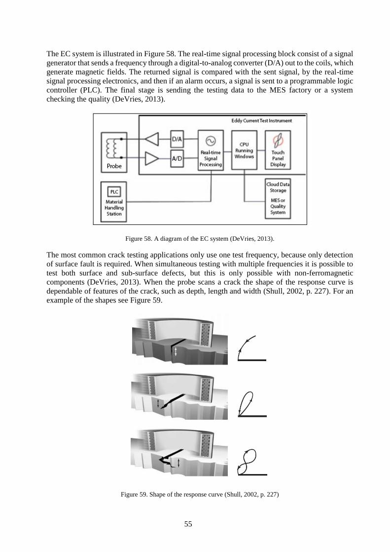
55

The EC system is illustrated in Figure 58. The real-time signal processing block consist of a signal

generator that sends a frequency through a digital-to-analog converter (D/A) out to the coils, which

generate magnetic fields. The returned signal is compared with the sent signal, by the real-time

signal processing electronics, and then if an alarm occurs, a signal is sent to a programmable logic

controller (PLC). The final stage is sending the testing data to the MES factory or a system

checking the quality (DeVries, 2013).

Figure 58. A diagram of the EC system (DeVries, 2013).

The most common crack testing applications only use one test frequency, because only detection

of surface fault is required. When simultaneous testing with multiple frequencies it is possible to

test both surface and sub-surface defects, but this is only possible with non-ferromagnetic

components (DeVries, 2013). When the probe scans a crack the shape of the response curve is

dependable of features of the crack, such as depth, length and width (Shull, 2002, p. 227). For an

example of the shapes see Figure 59.

Figure 59. Shape of the response curve (Shull, 2002, p. 227)

56

2.8.2 Equipment

There are a lot of different types of EC equipment, from handheld units to costume-designed

scanning systems. The handheld units showed in are used for measuring the conductivity thickness

of the material and to measure fault, such as cracks, pitting, corrosion, etc. The handheld devices

can have a variable frequency interval of 50 Hz – 8MHz. The device has a display that shows the

discontinuity response on a stripe chart. It is also possible to use a more complex EC system with

multiple probes for inspection of mass-produced parts. An automated EC crack system that detects

cracks is illustrated in Figure 60, which is used for automotive steering push rods (Shull, 2002, pp.

220-221).

Figure 60. EC inspection system (Shull, 2002, p. 221)

An instrument that offers high sensitivity, multi-frequency, direct measurement and versatility in

programming is the network/impedance analyzer. The disadvantages with this system are that it

can easily be damaged, it is expansive and experience is required (Shull, 2002, pp. 221-222).


Eddy current testing is a non-contacting method, which is a major advantage over e.g. ultrasonic,

dye penetrate and magnetic particle, which mean that no surface preparation is needed. The system

cost is relatively low compared to the X-ray system. Another advantage is that the method can be

used when the temperature is high. The system is portable and light weighted and there is no

concerns about the safety is needed. The resulting testing data can be stored and re-analyzed (Shull,

2002, pp. 264-265).

The disadvantages of the method is that the investigated material must be a conductor and that the

method is sensitive to a wide range of parameters, which increase the complexity of the analysis.

Eddy current testing is not applicable for ceramic gears (Shull, 2002, pp. 264-265).

57

2.9 Ultrasonic

The technique for ultrasonic monitoring is similar to the vibration monitoring, because both

systems monitor the noise generated by plant machinery or systems to determine the actual

operation condition of e.g. a gearbox. The difference between these systems is that ultrasonic

monitors the higher frequencies, e.g. ultrasound, produced by unique dynamics in the gearbox.

The normal monitoring range for vibration monitoring is lower than 1 Hz and up to 30 000 Hz.

The frequency range between 20 000 Hz and 100 kHz is monitored for the ultrasonic monitoring

(Mobley, 2002, p. 256).

The basic principal of ultrasonic testing of materials is the propagation and reflection of sound

waves. When using ultrasonic testing a probe is installed on the surface of the test-object. The

probe both transmit and receive the ultrasonic pulse. The probe transmit a short ultrasonic pulse

and the pulse is reflected and recorded as an echo, and if there is a cavity the returned echo will be

changed (MaterialsScience2000, 2014). For an illustration of the ultrasonic testing process see

Figure 61.

Figure 61. The process of ultrasonic testing (MaterialsScience2000, 2014)

2.9.1 Applications

Ultrasonic is primary used for airborne noise analysis, leak detection or material testing. These

applications are described below (Mobley, 2002, pp. 256-257).

AIRBORNE NOISE ANALYSIS

All plants are required by Occupational Safety and Health Administration (OSHA) regulations,

because ambient noise levels have to be met throughout the facilities. The primary used tool to

monitor the ambient noise levels and to ensure that the OSHA regulations are met is Ultrasonic

meters.

LEAK DETECTION

Leak detection is the most common application for ultrasonic monitoring. A leakage, i.e. turbulent

flow of e.g. liquids or gases through a restricted orifice, produces a high frequency signature. This

signature can be identified by using ultrasonic monitoring. Ultrasonic techniques are used when

detecting leaks in valves, steam traps, piping, and other process system.

58

MATERIAL TESTING

The ultrasonic technique is a primary test system for material testing. Test frequencies often start

at 250 kHz, or 250 000 cps (cycles per second), and up to 25 MHz, or 25 million cps. Testing of

materials consist of introducing of an energy source into the tested material. Then the

characteristics of the response are recorded by using ultrasonic instruments, e.g. striking a material

with a hammer and then the result is recorded with an accelerometer and ultrasonic meter. The

ultrasonic method relies on the measurement of time and amplitude or sometimes strength of a

signal between emission and reception. The sound will partly reflect at interfaces, this is because

of the mismatch of the acoustic properties between materials, e.g. the sound transmitted from steel

and reach a steel/air boundary will cause 99.9 % internal reflection, while if there is a steel/water

boundary only 88 % will be reflected within the material and then 12 % will be transmitted into

the water. A small crack in a compressive stress field that does not have faces that are oxidized

will lead to a steel/steel boundary, and therefore it is impossible to detect the crack using this

system. The steel/steel impedance ratios are the same and these must be different, otherwise it will

not be registered with ultrasonic.

2.9.2 System types

There are two different types of ultrasonic systems: structural and airborne. These systems provide

fast, accurate diagnosis of abnormal operations and leaks. The airborne ultrasonic detectors can be

used in both scanning and contact mode. When detecting a gas pressure leaks the scanners are

used, because these instruments are only sensitive to ultrasound and the user is not limited to just

one specific gas. For the contact mode it is a metal rod that acts as a waveguide. When the surface

is touched it is stimulated by high frequencies, ultrasound. These frequencies are stimulated on the

opposite side of the surface. The main idea of the system is to locate turbulent flow and restriction

in process piping. There is some of the ultrasonic systems that include transmitters that can be

mounted inside plant piping. Using this type of systems makes it possible for the monitors to detect

areas of sonic penetration along the container’s surface (Mobley, 2002, pp. 257-258).


The advantage with the method is that there are both contacting and non-contacting approaches,

e.g. laser generated/detected ultrasound can have a standoff distance of a couple of meters, but the

most common is transducer that must be in contact with the object. Ultrasonic is a flexible, portable

and robust method, and it can reveal subsurface flaw in the material of the test-object. Another

important advantage is that there are no environmental risk or health of the operator. Complex

geometries can be tested with an ultrasonic probe, but not all geometries (Shull, 2002, pp. 67-68).

The main disadvantage is that many ultrasonic systems are used as bearing condition monitors.

Unfortunately, it is not a valid method to determine the condition of rolling bearing, even if the

natural frequencies of rolling-element bearings will fall within the bandwidth of ultrasonic

instruments. The problem is that gear-meshing frequencies and other components will create

energy that cannot be separated from the bearing frequencies (Mobley, 2002, p. 258). Another

disadvantages is that the ultrasonic waves cannot report planar flaws, e.g. cracks that have its

length parallel to the wave travel direction. The method requires an experienced technician and in

some cases it can be expensive to operate (Shull, 2002, pp. 67-68).

59

2.10 Radiography testing

The radiographic testing is the oldest NDT method, and it was developed 1895 by Wilhelm

Röntgen. He found out that it was possible to see through a solid body, and named the method X-

ray because he used a form of radiation or rays. The radiography testing techniques makes it

possible to detect internal defects by subjecting the surface of the test-object to an X-ray, which

are high energy waves. If a defect, e.g. a void or an intrusion occurs, this will lead to a difference

of the density. Obtaining a digital image or an image on X-ray-sensitive film, can result in an

obtained radiograph of the structure. The attenuation of radiation differs for different materials,

and it is possible for shorter wavelengths to penetrate more through a material than longer

wavelength. Therefore it is important to know the density and the thickness of the material to

calculate how much exposure is needed for the production of a radiographic image of the test-

object. A thicker test-object needs more energy and a longer exposure time. For a schematic

illustration of radiographic testing see Figure 62. The technique is used to find internal cracks in

machine components (Mohanty, 2015, p. 162) (TWI, 2015) (Davies, 1998, pp. 120-121).

Figure 62. A schematic illustration of radiographic testing (Davies, 1998, p. 121)

2.10.1 Description of X-rays

X-rays are waves that are electromagnetic, and their energy is 100-100 000 times higher than

visible light. For the properties of the X-rays compared to other electromagnetic spectrum see

Figure 63. X-rays can be both absorbed and scattered by a material, but it is possible for rays to

pass through some materials because of its high energy. When using X-rays it is possible to yield

data in one-dimension (1-D), gauge measurement, two-dimensions (2-D), radiograph, two-

dimensional slices or three spatial dimensions (3-D), computed tomography. When measuring the

attenuation along a straight beam path is often called X-ray gauging, this results in a single data

point. With this system it is possible to define the thickness of a material if both the composition

and the mass density of the material are known, while the two-dimensional projection radiography

is used within medicine and NDE (Shull, 2002, pp. 344-347).

Figure 63. Values of the electromagnetic spectrum (Shull, 2002, p. 345)

60


The advantages with radiographic testing is that is works on almost all materials and it is a fast

area inspection. With this method it is possible to examine the interior of the test-object, which

mean that the system can reveal subsurface flaw in the material of the test-object and it is visual.

The testing method can give information about the composition of the material, e.g. density,

volume, mass and thickness (Shull, 2002, pp. 511-512).

The main disadvantage is that the method creates serous safety concerns, because the radiation is

dangerous and the operator has to be highly skilled and be experienced. It is an expensive method

and it is not possible to detect closed cracks (Shull, 2002, pp. 511-512).

2.11 Acoustic Emission

Acoustic emissions are small vibration pulses, elastic waves that are emitted from a variety of

mechanisms, e.g. crack formation and propagation, fretting, plastic deformation and phase

transforms. These emission pulses have a frequency in the range of 20 kHz to 1 MHz. Acoustic

Emission (AE) is a system used to examine these emissions, by recording and analyzing them.

This method is used in material research and when testing and inspecting different structures. AE

can be divided into different areas: material research, inspection and testing of components and

structures, continuous monitoring of structures and production quality control (Bindt, 2013)

(Gupta & Karma, 2014) (Almkvist, 2015). The difference between AE and other NDE methods is

that the measured signals are produced within the material of the tested component (Shull, 2002,

p. 366).

A sudden change in stress and displacement of material occur with a propagation of a crack, and

the variation of the stresses and strains act as stress wave sources. If the change of stress is large

and rapid, elastic waves will radiate away from the crack. The elastic waves carrying a portion of

the energy from the source. The acoustic emission waves can be detectable by using piezo-electric

transducers mounted on the machine. The waves can provide an early warning of impending failure

if the waves are efficiently detected. Acoustic emission has been used for many different

applications: detect flaws in nuclear vessels and chemical tanks, condition monitoring and also

when studying fatigue failures in gears (Singh, et al., 1999).

2.11.1 Potential of AE

AE monitoring is applicable for a variety of applications: damage activity monitoring, damage

mechanism identification, damage location and strength predictions (Shull, 2002, p. 372).

DAMAGE ACTIVITY MONITORING

When monitoring the damage activity an indication of the acoustic emission activity, e.g. the

number of signals or RMS voltage output from a sensor is recorded, which means that individual

signals are not analyzed and documented. The activity of the AE indicate if a damage has occurred.

The best measuring result is accomplished if there are little or no background noise, e.g. EMI or

structural vibrations. The monitoring can be used when determining a maximum load or stress

applied to a structure (Shull, 2002, p. 372).

DAMAGE LOCATION

To locate a damage the acoustic activity is monitored by an array of sensors. The location of the

sensors are important to collect the signals from the damage. Using sensors can lead to cost savings

in comparison to e.g. fully scanning where point sensors are used (Shull, 2002, p. 378).

61

DAMAGE MECHANISM IDENTIFICATION

The damage mechanism, identification is the most difficult task when it comes to AE analysis,

because of the present of multiple damage mechanism and noise sources. It is difficult to identify

the source when the AE signal changes when it propagate. The identification of the source aids in

noise discrimination and rejection, which result in an improvement of the AE data quality. To

attempt identification of the source it is important to have knowledge about the test structure’s

characteristics, e.g. the geometry and the material elastic properties, sensors and measurement

system and also knowledge about the effects of the wave propagation (Shull, 2002, p. 378).

STRENGTH PREDICTIONS

The AE monitoring method results in estimated information about the strength or life of a structure.

However, the disadvantage with the estimation is that there are no direct physical connection

between strength and AE. Most of the strength assessments from the AE monitoring are based on

empirical correlations. These correlations comes from failure tests of identical structures (Shull,

2002, pp. 378-379).

2.11.2 The principal of acoustic emission

The process of acoustic emission starts with a force acting on a body, and the stresses causes

deformation which lead to acoustic emission. The stresses acting on the test-object results in plastic

deformations, which lead to breakdown of the material. The breakdown produces acoustic

emission, an elastic wave that travel from the source, moving through the body and to an AE

sensor. Then the sensor produce an electrical signal that travels to electronic equipment, where it

is processed. The sensors are the most vital part of an acoustic emission system (Hellier, 2003, p.

536).

The sensors are connected to the data acquisition system. The main purpose of the sensors is to

convert the mechanical motion of the surface of the test-object into an electrical signal. This signal

is then recorded and analyzed. When converting the motion the sensors using a phenomenon called

piezoelectric effect. When some materials are subjected to a force they will redistribute the charge

in the material, and it will result in voltage across the material. A connection between the sides of

the material to an electrical system means that this voltage can be measured. Therefore, it is

possible for the material’s acceleration can be turned into an electrical signal (Singh, et al., 1999).

For a schematic of the acoustic emission process see Figure 64.

Figure 64. The process of Acoustic Emission monitoring (Hellier, 2003, p. 536)

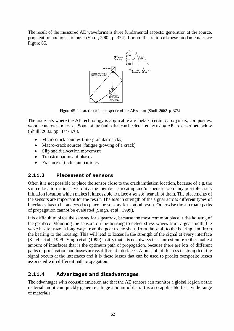
62

The result of the measured AE waveforms is three fundamental aspects: generation at the source,

propagation and measurement (Shull, 2002, p. 374). For an illustration of these fundamentals see

Figure 65.

Figure 65. Illustration of the response of the AE sensor (Shull, 2002, p. 375)

The materials where the AE technology is applicable are metals, ceramic, polymers, composites,

wood, concrete and rocks. Some of the faults that can be detected by using AE are described below

(Shull, 2002, pp. 374-376).

Micro-crack sources (intergranular cracks)

Macro-crack sources (fatigue growing of a crack)

Slip and dislocation movement

Transformations of phases

Fracture of inclusion particles.

2.11.3 Placement of sensors

Often it is not possible to place the sensor close to the crack initiation location, because of e.g. the

source location is inaccessibility, the member is rotating and/or there is too many possible crack

initiation location which makes it impossible to place a sensor near all of them. The placements of

the sensors are important for the result. The loss in strength of the signal across different types of

interfaces has to be analyzed to place the sensors for a good result. Otherwise the alternate paths

of propagation cannot be evaluated (Singh, et al., 1999).

It is difficult to place the sensors for a gearbox, because the most common place is the housing of

the gearbox. Mounting the sensors on the housing to detect stress waves from a gear tooth, the

wave has to travel a long way: from the gear to the shaft, from the shaft to the bearing, and from

the bearing to the housing. This will lead to losses in the strength of the signal at every interface

(Singh, et al., 1999). Singh et al. (1999) justify that it is not always the shortest route or the smallest

amount of interfaces that is the optimum path of propagation, because there are lots of different

paths of propagation and losses across different interfaces. Almost all of the loss in strength of the

signal occurs at the interfaces and it is these losses that can be used to predict composite losses

associated with different path propagation.


The advantages with acoustic emission are that the AE sensors can monitor a global region of the

material and it can quickly generate a huge amount of data. It is also applicable for a wide range

of materials.

63

The disadvantages is that the implementation of acoustic emission analysis is quite difficult,

because the propagation of acoustic wave in solids is complicated and the occurrence of multiple

modes that propagate with different velocities, reflection, etc. can affect the measured signal.

Another limitation is that the emitted acoustic signal depends on the characteristics of the source

within the material, and the characteristics differ. Even the same AE source can result in different

received signals, because of the transportation path of the signal to the measuring instrument

(Singh, et al., 1999).

2.12 Magnetic Particle Inspection

When choosing to use the magnetic particle inspection (MPI) three further decisions have to be

made, and these are described below (Shull, 2002, p. 191).

Which magnetizing method is the most appropriate?

Which type of current should be used?

Whether to use wet particles or dry ones?

The system of magnetic particle inspection is quite simple, see Figure 66. The test-object is

magnetized by placing it between two electro magnets. If the test-object is free from defects the

magnetic field lines run within the test-object and parallel to its surface, and if the test-object is

defected the magnetic field lines will locally leave the surface and a leakage field occurs. When a

suspension of ferromagnetic particles are applied over the surface of the test-object the

ferromagnetic particles will run off at defect free areas and they are attracted and clustered near

defects. After the ferromagnetic particles have been applied the cracks can be seen as dark lines

on the surface of the test-object, but with UV-light the lines become more visible

(MaterialScience2000, 2014).

Figure 66. The magnetic inspection process (MaterialScience2000, 2014)

The sample must be magnetized before magnetic particle inspection, which mean that this system

is limited to components that are easy to magnetize. The components that have a high relative

permeability of 100 or over 100 can be used, which is e.g. copper, brass, aluminum, titanium and

austenitic stainless steel (Shull, 2002, pp. 191-192). For a magnetic particle inspection of a gear

wheel see Figure 67.

Figure 67. Magnetic particle inspection of a gear wheel (MaterialScience2000, 2014)

64

2.12.1 Theory

The ability of a magnet that attracts or repels other magnets or pieces of metal is called magnetic

effect. A bar magnet consist of two points of concentrated effect: north and south poles. Opposite

poles attract each other, while like poles repel. There is no poles if the bar magnetic is bend into a

circle, but a small crack will make the magnetic field leave the circle at a north pole and return at

a south pole, see Figure 68 (Shull, 2002, pp. 194-195).

Figure 68. Circular magnet (Shull, 2002, p. 194)


Magnetic particle inspection is a reliable system for finding cracks of surfaces and especially if

the cracks are very fine and shallow, the method is easy to operate and it produces indications that

are easy to understand. A skilled and experienced operator can easily detect the depth of cracks

with high accuracy. With this testing method there is no limitations when it comes to size and

shape of the test-object, and it is possible to detect limited sub-surfaces defects to a maximum

depth of about 6.35 mm (Shull, 2002, pp. 193-194).

The disadvantages are that it can only be used on ferromagnetic parts, it only detects surface or

near-surface cracks and electrical arcing or burning can occur at the contact points during the

testing of the machine. Another limitation with this method is that the object must be demagnetized

after the process and some of the parts need individual handling. When using this method it is

sometimes required that the test-object and the testing instrument is in contact and it is not enough

with just one inspection (Shull, 2002, pp. 193-194).

65

THE PROCESS

In this chapter the working process is described. The process of the project is divided in four

phases and the chapter begins with the first phase, which is the planning where Scania’s current

solution is described. During the second phase, the specification of requirements where developed

and the methods available on the market where examine. The third phase consist of the system

evaluation. This chapter ends with a detailed design of the final system.

3.1 Phase 1 - Project planning

This section of the report present the result of the pre-study performed during the project planning

phase and also describe Scania’s current solution. The sub-phases for phase 1 are shown in Figure

69.

Figure 69. Phase 1 – Project Planning

3.1.1 Planning

The first phase of the project was to plan and make a schedule of the different parts of the project.

The schedule used in this project was a Gantt chart. A Gantt chart display the activities in a project

against time. Each activity and its duration is showed in the chart, which gives a good overview of

a project (Gantt, 2015).

3.1.2 Scania’s current solution

Today Scania is using two different systems to detect damages in the gearbox: A control/measuring

and regulation system from Scania that is integrated in the test-rigs and delta-ANALYSER from

Reilhofer.

THE CONTROL/MEASURING AND REGULATION SYSTEM

The system consist of a central control-PC with a STP-application, a Labview based control

system, that communicate with the object via PROFIBUS (PROFIBUS = Process Field Bus) and

CAN-bus (CAN = Controller Area Network). The PROFIBUS has functions for the variable

frequency drive control system, cooling/heating system, safety system, ventilation and distributed

I/O nodes. CAN-bus is a bus-system for data exchange which is designed for use in the vehicle,

and it is controlling the OPC-system of the gearbox.

66

The sensors connected to the measuring plint are thermocouple (TC), temperature sensor (PT100),

external revolution sensor, oil pressure sensor and vibration sensor (Prytz, 2008). For the sensors

see Figure 70.

Figure 70. The sensors for the control/measuring and regulation system

STP controlling system

Scania CV AB has developed a Labview based control system called STP (Scania Test Platform).

The main purpose of the system is to control the components of the test-rig and also make it easier

for the operator. With this system it is possible to measure the vibration, temperature, input and

output torque, oil pressure, etc. (Prytz, 2008).

There are different states of the STP: off, monitor, manual and auto. The test-rig is in state off

when it is in start-up and after any faults. This is not a normal operating mode. The entire software

will reboot itself if the STP is in off mode. In monitor mode, the rig is completely shut off but the

control system software is running (Einarsson, 2011.

67

In manual mode, the rig can be operated manually, which mean that both ventilation and oil

condition systems is running in this mode. All of the control system critical alarm limits are

monitored, and the engines and the tilting device can be started by the operator (Einarsson, 2011).

For the control panel used in manual mode see Figure 71.

Figure 71. Control panel in the control room: 1: Emergency stop, 2: Gear shifting unit, 3: Watchdog, 4: RPM rear

machine, 5: Torque rear machine, 6: RPM front machine, 7: Torque front machine.

In auto mode, the test sequence that is specified in the test protocol will be run. The system will

only enter the auto mode if the operator is in manual mode, and the system will return to manual

when the test sequence is finished (Einarsson, 2011). The states of the STP and its transitions are

presented in Figure 72.

Figure 72. The STP-states (Einarsson, 2011)

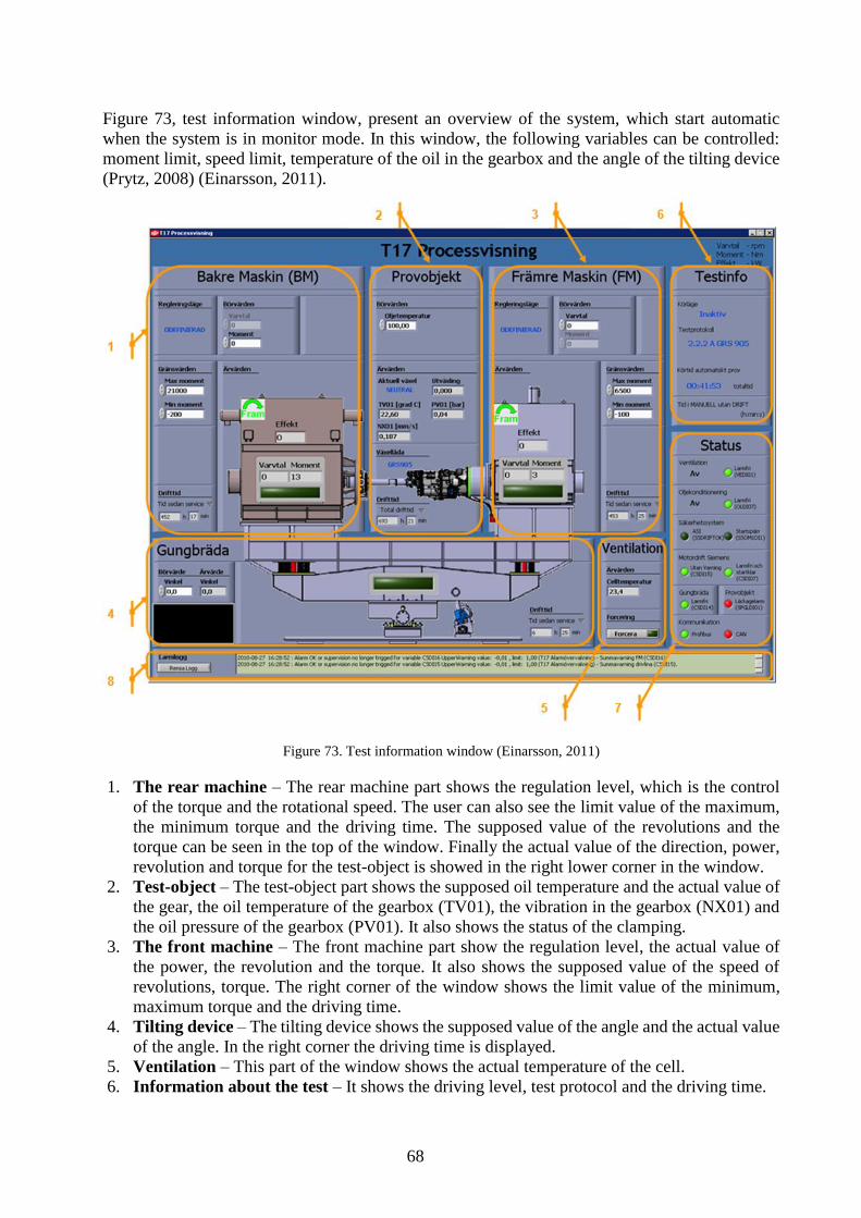
68

Figure 73, test information window, present an overview of the system, which start automatic

when the system is in monitor mode. In this window, the following variables can be controlled:

moment limit, speed limit, temperature of the oil in the gearbox and the angle of the tilting device

(Prytz, 2008) (Einarsson, 2011).

Figure 73. Test information window (Einarsson, 2011)

1. The rear machine – The rear machine part shows the regulation level, which is the control

of the torque and the rotational speed. The user can also see the limit value of the maximum,

the minimum torque and the driving time. The supposed value of the revolutions and the

torque can be seen in the top of the window. Finally the actual value of the direction, power,

revolution and torque for the test-object is showed in the right lower corner in the window.

2. Test-object – The test-object part shows the supposed oil temperature and the actual value of

the gear, the oil temperature of the gearbox (TV01), the vibration in the gearbox (NX01) and

the oil pressure of the gearbox (PV01). It also shows the status of the clamping.

3. The front machine – The front machine part show the regulation level, the actual value of

the power, the revolution and the torque. It also shows the supposed value of the speed of

revolutions, torque. The right corner of the window shows the limit value of the minimum,

maximum torque and the driving time.

4. Tilting device – The tilting device shows the supposed value of the angle and the actual value

of the angle. In the right corner the driving time is displayed.

5. Ventilation – This part of the window shows the actual temperature of the cell.

6. Information about the test – It shows the driving level, test protocol and the driving time.

69

7. Status – It shows the status of the test-object, information about the ventilation, oil, safety,

motor, the tilting device and the communication (Profibus and CAN).

8. Logging of the Alarm – Shows the alarms of the test-object.

Great forces will be developed during the test, therefore it is important that the test-rig stop when

something goes wrong. In the STP it is possible to create parallel monitoring processes and to

monitor the same variable in several places. Figure 74 show an example of the limits for the

temperature of the oil out of the gearbox, where the upper limit is 155, and the upper warning is

150. There are five different permanent monitoring systems: alarm monitoring, safety monitoring,

OptiCruise monitoring, secure operation monitoring and user specified monitoring (Einarsson,

2011).

Alarm monitoring – Stops the test-rig when something critical occur.

Safety monitoring – Stops the test when the motors or the test-object are overloaded.

OptiCruise monitoring – Stops the test-rig when there is something wrong with the

communication to the OptiCruise-unit.

Secure operation monitoring – Stops the test-rig if it is not possible to insure a safe

operation.

User specified monitoring – Stop the rig to protect the test-object and it is based on the

limits set by the operator, where the test-object’s absolute maximum limits for torque,

speed, pressure, temperature and vibration are set. When the test-rig stop because the limits

are exceeded it is possible to see what happened before the stop by using the post-mortem,

which dumps the last minute’s values for selected variables to a text file.

Figure 74. User specified monitoring

The variables, such as the oil temperature in and out of the gearbox, the oil pressure, the moment

and the speed, are plotted in real time during the test, see Figure 75. The power losses are also

measured during the test, by measuring the power in and out. The losses can also indicate that the

gearbox is defected. The operator specifies the measurement variables to be monitored and if any

of the measured variables exceed the motors will automatically be shut off and the test will be

stopped, e.g. the oil pressure should be about 2.3 bar to 2.8 bar during the test and if the test is

70

stopped the operator will get a text message with information about the test and the exceeded

measurement variables.

Figure 75. Test results for the third gear high split: MPPT01 = Oil temperature into the gearbox, TV01 = Oil

temperature out of the gearbox, PV01 = Oil pressure, NX01 = Vibration, NX01 gräns = Vibration limit

DELTA-ANALYSER FROM REILHOFER

Delta-ANALYSER is a measuring system developed by Reilhofer, which is used for early stage

detection of acoustic noise emitting machines, such as gearboxes. It detects failure of a machine

by comparing the tested gearbox vibration behavior to a previously built reference (Reilhofer,

2014).

The system consists of a measuring system and a PC which visualizes the collected data. Measured

signals, such as structure-born noise and rotational speed, are recorded by the system (Reilhofer,

2014).

Every test run with the system is defined by a test-list, a collection of the different load-steps.

These load-steps are defined by a valid range of the signal, such as rotational speed, torque,

temperature, gear information etc. and also settings, such as the alarm threshold (Reilhofer, 2014).

Delta-ANALYSER provides the user with two software modules: setting and monitoring software

and evaluation software. The setting and monitoring software control and measuring the device,

while the evaluation software analyze and evaluate the measured data (Reilhofer, 2014).

Measuring

The noise collected by the measuring system evolves inside the gearbox by intertwining of the

rotating parts, e.g. gear wheels or bearings. The noise is transmitted over the shaft and the bearings

to the sensor, in form of structure-born noise, the sound generated from a vibrating source, see

Figure 76 (Reilhofer, 2014) (Head-acoustics, 2015).

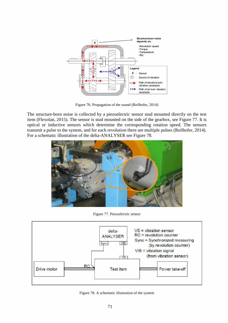
71

Figure 76. Propagation of the sound (Reilhofer, 2014)

The structure-born noise is collected by a piezoelectric sensor stud mounted directly on the test

item (Flexolan, 2015). The sensor is stud mounted on the side of the gearbox, see Figure 77. It is

optical or inductive sensors which determine the corresponding rotation speed. The sensors

transmit a pulse to the system, and for each revolution there are multiple pulses (Reilhofer, 2014).

For a schematic illustration of the delta-ANALYSER see Figure 78.

Figure 77. Piezoelectric sensor

Figure 78. A schematic illustration of the system

72

Analyzing and evaluation

A spectrum is calculated from the measured signal of the structure-born noise. This is made via

Fast Fourier Transformation (FFT), which is an algorithm to compute the Discrete Fourier

Transform (DFT) and its inverse, which means that the FFT method converts time-based spectra

to frequency-based. The system consists of two different analysis methods: frequency analysis and

order analysis. The order analysis determines how often an event occurs per revolution, and for

the frequency analysis it is crucial how often an event occurs per second. An order spectrum is

independent of speed, and when analyzing the order spectrum it is easier to obtain side bands using

only the Frequency Analysis (Reilhofer, 2014).

When testing a gearbox there is a learning phase in the beginning of each measurement. The first

step of the measurement consists of developing a reference for each spectral line, and also an upper

and lower tolerance is calculated by means of a statistical procedure. The second phase is called

the Mix phase, where the reference and the tolerances are refined. The monitoring of the test items

starts at the same time. In both the mixed phase and also the monitoring state, the current spectrum,

showed in Figure 79 diagram a), is an average of a number of single measurements. Continuously

the current spectrum is compared to the reference. An entry is made in the Deviation spectrum,

see Figure 79 diagram c), if the amplitude of a spectral line not meets the tolerance range. Then

the deviation spectrum is summed up to a trendindex, see Figure 79 diagram d). The trendindex is

compared to an alarm threshold, and if the alarm value exceeds the test bench will be switched off.

According to Reilhofer the system will switch off early enough to analyze the defects and also the

original cause of the damage (Reilhofer, 2014).

Figure 79. Trendindex (Reilhofer, 2014)

73

The test item, e.g. gear wheel, bearing etc. can be assigned to an order and also the specific line of

the order spectrum can be calculated accurately and therefore it is possible to locate the cause. An

example of how bearing changes and also the gear defects are illustrated in a waterfall diagram,

see Figure 80 (Reilhofer, 2014).

Figure 80. Waterfall diagram (Reilhofer, 2014)

Figure 81 represent the trendindex of a defected sun gear for a planetary gear test from Scania and

in Figure 82 a waterfall diagram of the same gear is presented.

Figure 81. Trendindex: Planetary gear test, third gear high split damage progression

74

Figure 82. Waterfall diagram: Planetary gear test, third gear high split

The damage orders for each transmission components are pre-calculated and saved to a database,

by using a program called Order calculator. In the Order calculator a transmission definition is

created by using a graphical user interface, and for a heavy tipper gearbox transmission definition,

see Figure 83. The created transmission definition is then used during tests of the “pattern

recognition”, an advanced analysis method, to calculate the probability of error for each

component.

Figure 83. Order Calculator

75

Advantages and disadvantages

The advantages and disadvantages of delta-ANALYSER is described below:

Advantages Disadvantages

The order calculation, where a gearbox

is schematically drawn with e.g. the

order of the gears, can be connected

with the waterfall diagram. This makes

it easier to distinguish the order of a

fault.

Delta-ANALYSER has an alarming

system.

The waterfall diagram is detailed,

which makes it possible to examine

every minute of the test.

An engineer from Reilhofer is coming

about 3 times per year to check the

system.

The database-files can be send to

Reilhofer in Germany for examination.

The algorithms for the trendindex is not

accessible for Scania.

Knowledge about how the gearbox

works, to able to understand the lines.

Every gearbox does not act the same,

there are always some differences.

Therefore the result of the

measurements can be false. Probability

of correct measurements ~70 %.

No virus protection for the PC.

It is not possible to make an exact copy

of the gearbox in the order calculation

program, there are some deviations

from reality.

Assistance from Reilhofer is needed.

Delta-ANALYSER’s alarming system

is not used by Scania.

If the hardware is upgraded, Scania has

to pay to continue with the system.

Overlapping orders, which makes it

difficult to find the damage because

bearings and gears have the same

orders.

3.1.3 Phase 1 - Conclusion

The main disadvantage with the current system used by Scania, delta-ANALYSER and the STP,

is their unreliability. It is not possible to use delta-ANALYSER’s alarming ability, because the

system is not accurate enough and it is difficult for the operator to distinguish a defect by using

these systems. Scania needs a more accurate and reliable system to stop the endurance test in the

right time and a system that can predict the development of the defect.

76

3.2 Phase 2 – Research

This section of the report present the result of the research, and evaluation of the condition

monitoring methods. The sub-phases for phase 2 are shown in Figure 84.

Figure 84. Phase 2 – Research

3.2.1 Persona

The information for the persona was gathered by interviews with the employees. The chosen target

group was men between 30-65 years old, who working as test engineers and operate the test-rigs

at Scania. The persona gave a better understanding of the customer’s needs. For the persona see

Appendix D.

3.2.2 System requirements

The first step when selecting the most appropriate technique for Scania CV AB was to develop a

list of specific features or capabilities of the system. The requirements of the system have been set

through meetings and discussions with Scania CV AB, and by investigating the capabilities that a

chosen system must have according to Keith Mobley, 2001, p.877-879. A document of the system

requirements has been specified, and it was used when evaluating the different systems, see Table

7. For a description of each requirement, see Appendix E.

Table 7. System Requirements

Row # Requirements Weight

Per

form

an

ce

1 The system shall be easy to access in the test-rig, 10 min 3

2 The system shall be easy to maintain and service 3

3 The system shall have a user-friendly software and hardware 5

4 The system shall provide the user with accurate result 4

5 The system should provide the user with automated data acquisition 4

6 The system shall be reliable 5

7 The system shall provide the user with automated data management

and trending 5

8 The system shall be flexible 4

9 No expertise shall be needed to operate the system 3

10 The system shall be alert and alarm if a limit is reached. 5

77

11 The system shall have a data storage 5

12 The system shall be user-friendly to operate 4

13 The system shall have automatic trending 4

14 The system shall be able to handle high temperatures (oil

temperature = 100°C) 4

15 The system shall simplify diagnostic of the gearbox 4

Com

pan

y c

on

stra

ints

16 The test shall stop if a damage of a bearing has reached a specific

size specified by Scania 5

17 The test shall stop if a damage of a gear has reached a specific size

specified by Scania 5

18 The system shall be able to use for all the different types of

gearboxes at Scania 4

19 The gearbox must be unaffected in terms of function and strength 5

Main

ten

an

ce

20 The system shall provide the user with easy access to the parts that

require maintenance, less than an hour 3

21

No need for special tools 3

Syst

em

Lif

e S

pan

22 The system shall be in production for 10 years

3

Safe

ty

23 The system shall protect the safety of the employees 5

24 No heavy lifting > 8 kg 4

Inst

all

ati

on

25 Installation Instructions 3

26 Scania standards for the components (TFP - Technical regulations

for machinery production equipment) - 2011-12-29 5

Docu

men

tati

on

27 Training and technical support shall be provided 4

28 Operation instructions shall be provided 5

29 Instruction on how to disassembly the system shall be provided 2

30 Instructions on how to recycle the parts shall be provided 3

31 The system shall provide the user with an automatic report 4

Co

st

32 Operating cost 4

33 System cost 4

78

3.2.3 Function tree

In the function tree the main function was divided into four groups: hardware, software, company

and the whole system and these groups were divided into sub-functions and then every sub-

function was divided into new sub-functions. The function tree was based on the system

requirements, see Figure 85.

Figure 85. Function tree

79

3.2.4 Research results

Table 8 summaries the advantages and disadvantages of the condition monitoring methods on the

market. The condition monitoring methods found during the research part of the project is

described in chapter 2, frame of references.

Table 8. Advantages and disadvantages of the methods

Method Advantages Disadvantages

Vibration The vibration analysis reacts

directly to changes.

Applicable to both linearly and

nonlinearly moving equipment.

Used for controlling the quality,

detect cracks and to analyze the

flow of fluid.

Possible to locate the source of

the defect.

Background noise

Installation

Thermography The test-object and the

component do not have to be in

contact.

Cost

Atmospherically effects

Components both emit and

absorb the transmitted

infrared energy.

Factors can affect the

component’s infrared

energy emitting ability,

e.g. surface conditions and

coatings.

Difficult to measure the

temperature inside the

gearbox.

Oil analysis Easier to keep the oil clean.

Early indication that something

has happened.

Early detection of a damage,

such as an early beginning of

pitting or spalling.

Expensive

Understanding the analysis

result.

Difficult to locate the

failing component.

Acoustic

Emission AE sensors can monitor a global

region of the material.

Can generate a huge amount of

data quickly.

It is applicable for a wide range

of materials.

Installation

The occurrence of multiple

modes that propagate with

different velocities,

reflection, etc. can affect

the measured signal.

Ultrasonic There are both contacting and

non-contacting approaches

Requires an experienced

technician.

The ultrasonic waves

cannot report planar flaws.

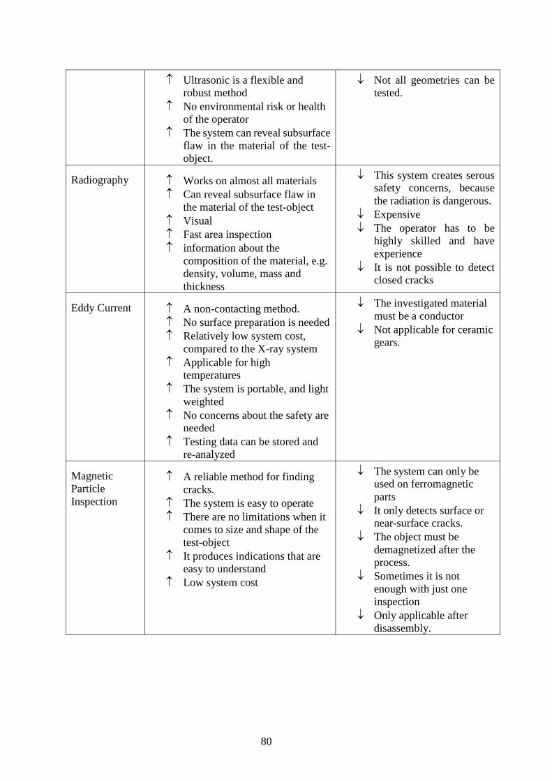
80

Ultrasonic is a flexible and

robust method

No environmental risk or health

of the operator

The system can reveal subsurface

flaw in the material of the test-

object.

Not all geometries can be

tested.

Radiography Works on almost all materials

Can reveal subsurface flaw in

the material of the test-object

Visual

Fast area inspection

information about the

composition of the material, e.g.

density, volume, mass and

thickness

This system creates serous

safety concerns, because

the radiation is dangerous.

Expensive

The operator has to be

highly skilled and have

experience

It is not possible to detect

closed cracks

Eddy Current A non-contacting method.

No surface preparation is needed

Relatively low system cost,

compared to the X-ray system

Applicable for high

temperatures

The system is portable, and light

weighted

No concerns about the safety are

needed

Testing data can be stored and

re-analyzed

The investigated material

must be a conductor

Not applicable for ceramic

gears.

Magnetic

Particle

Inspection

A reliable method for finding

cracks.

The system is easy to operate

There are no limitations when it

comes to size and shape of the

test-object

It produces indications that are

easy to understand

Low system cost

The system can only be

used on ferromagnetic

parts

It only detects surface or

near-surface cracks.

The object must be

demagnetized after the

process.

Sometimes it is not

enough with just one

inspection

Only applicable after

disassembly.

81

3.2.5 Benchmarking

There are many online condition monitoring systems on the market, and most of these systems

within each condition monitoring method are fairly the same. In Table 9 the companies and their

techniques are presented. The main purpose of the benchmarking was to found companies that

offer systems based on the different methods described in chapter 2.

Table 9. Suppliers and their condition monitoring methods

Suppliers Method Short description

ABB Vibration ABB provide companies with solutions

for monitoring and diagnose the condition

of the machinery. They have products that

can measure the vibration data and

diagnose the system. The company has

experience of condition monitoring of

mostly rotating machinery (ABB, 2014).

ARGO HYTOS Oil analysis ARGO HYTOS offer solutions for fluid

power technology. They have a wide

modular product range, which makes it

possible for design specialized the

systems for each customer (ARGO-

HYTOS, 2014).

Askalon AB Vibration Askalon can offer different systems for

condition monitoring of rotating

machinery. They help the customer to

build the system and to procedure the

analyzing for monitoring the machinery

(Askalon, 2014).

CREO Dynamic Ultrasonic/Acoustic

Emission

CREO Dynamics was started 2010 in

Linköping, Sweden. They offer NDT

methods and solutions, and they have their

root in the aerospace industry (CREO,

2014).

Colly Filtreringsteknik

AB

Oil analysis Colly Filtreringsteknik AB offer their

customers oil analyzing solutions (Colly,

2015).

Dekra NDT Systems (Eddy

Current testing, Magnetic

Particle Inspection,

Ultrasonic testing and X-

ray Inspection)

Dekra is specialized in non-destructive

methods for examine the condition of the

machinery, which will lead to prevention

of catastrophic failures (Dekra, 2014).

DISCOM Vibration Discom is offers vibrations systems for

industrial machinery. Their system has

been used for testing automobile

components, such as gearboxes and

engines (DISCOM, 2012).

82

eMaintenance Vibration and

Thermography

eMaintenance is a small company that has

developed a decision system called

eMDSS for condition monitoring. The

system is applicable for both vibration and

thermography systems.

FLIR Thermography FLIR is a world leading company in

thermal imaging and infrared cameras.

They offer cameras for industrial

machinery applications (FLIR, 2015).

Fluke Thermography Fluke offers infrared cameras and

thermometers for condition monitoring of

industrial machinery (Fluke, 2014).

Hydac Oil analysis Hydac offers a wide range of products,

such as fluid control products, valves,

hydraulic accumulators, etc. for all

different kind of industries (Hydac, 2015).

Mistras Acoustic Emission Mistras provides their customers with

non-destructive testing systems, software,

NDT measuring instrument, etc. (Mistras,

2014).

MLT Eddy Current/Vibration MLT (Maskin & Laserteknik AB) is a

reseller of Prüftechnik, an international

company. They offer systems for vibration

monitoring (MLT, 2015).

MTS Systems Norden

AB

Oil analysis MTS offers products for monitoring and

analyzing the fluid in the machinery. They

design product for a wide range of

applications: automobile, aircraft, bridges

and buildings (MTS, 2014).

NORELLS

Termografi AB

Thermography NORELLS Termografi AB offers IR

cameras for condition monitoring

(NORELLS, 2007).

Parker Hannifin Oil analysis Parker Hannifin is a world leading

company that offer control technologies

and systems. They provide their customers

with condition monitoring systems for

industrial and aerospace markets (Parker,

2015).

SKF Acoustic Emission/

Vibration

SKF is a worldwide manufacturer of

bearings, but they also offer systems for

condition monitoring. The company offers

acoustic emission systems and vibration

systems (SKF, 2015).

After contacting the companies it was verified that not all of the companies had systems that were

suitable when monitor the gearbox. The current thermography systems is not suitable, because it

83

is not possible to mount cameras inside the gearbox during the testing, and if the cameras are

mounted outside it will only be possible to measure the temperature of the gearbox housing.

According to CREO, ultrasonic is difficult to use when monitoring gearboxes, because of the

background signals, and it is more difficult to install the ultrasonic sensors than the vibration

system sensors.

Dekra have non-destructive methods, such as Eddy Current testing, Magnetic Particle Inspection,

Ultrasonic testing and X-ray Inspection. The disadvantages with their eddy current system is that

it is not applicable when testing the gearbox in the test-rig, but it is possible to use the method

when testing gears and bearings after the disassembly of the gearbox. The magnetic particle

inspection is also a method that can be used after disassembly. The X-ray Inspection can create

serious health concerns for the operator, which mean that a lot of preparation have to be done

before installation.

One of the systems used by Scania, delta-ANALYSER, is based on vibration. Ultrasonic, acoustic

emission and vibration are all based on noise, and the systems are similar. According to Daniel

Bäckström, Scania, it is possible that the same problems as with delta-ANALYSER will remain if

Scania start using acoustic emission and ultrasonic.

SKF presented a vibration system, used for testing truck gearboxes by Volvo in Eskilstuna, and

according to SKF the system can detect damages in an early stage.

eMaintenance described their decision system, that is based on an algorithm developed by Basim

Al-Najjar. According to eMaintenance the decision system would be applicable for the existing

system used by Scania. Their system called eMDSS would make it easier to locate the source of a

defect and it can also predict the development of the source.

3.2.6 Pugh matrix

The current condition monitoring methods and systems were evaluated in a simplified Pugh

matrix, because more information is needed to accomplish a more detailed Pugh matrix. The

methods were compared with the system currently used by Scania, delta-ANALYSER and STP.

For the Pugh matrix see Figure 86.

Figure 86. Simplified Pugh Matrix

84

3.2.7 Phase 2 - Conclusion

After an internal discussion, where the system requirements, benchmarking and the result of the

Pugh matrix were taken in account, it was decided to continue investigating the oil analysis

systems, compare the vibration system from SKF with the current measuring system, delta-

ANALYSER, from Reilhofer and also continue investigating the system from eMaintenance.

A combination of vibration and oil analysis is required, because one single method does not

support all needed requirements, e.g. it is not possible to locate the source of the defect with the

oil analysis systems available today if the components is made of the same material, which is an

important requirement of the system, see Table 7.

In Figure 87 a chart is presented that show the condition monitoring methods’ pre-warning time

of failure. The y-axis is the the condition of the test-object and the x-axis is the time. The black

line describe the condition of the machinery, where the condition is perfect on the far left, and then

moving to damage initiation and finally failure. By combining a vibration system and the oil

analysis system, the earliest warning of damage initiation can be given.

Figure 87. Condition monitoring methods’ pre-warning time of failure (Parker, 2014)

85

3.3 Phase 3 - System evaluation

This section of the report present the evaluation of the chosen systems. The sub-phases for phase

3 are shown in Figure 88.

Figure 88. Phase 3 – System evaluation

3.3.1 Evaluation of chosen system

Vibration and oil analysis where chosen after an internal discussion at Scania. Oil analysis

companies, SKF and eMaintenance were contacted and they presented their systems that were

applicable for a gearbox. Most of the oil analysis companies had systems based on oil particle

counting. The companies and their systems are presented in Table 10. The purpose of the

benchmarking was to find online or inline systems, which means that offline system has been

discarded.

Table 10. Chosen suppliers and their systems

Supplier Method System Online or Inline

SKF Vibration Vibration Online

eMaintenance Vibration Decision system for

vibration

measurement

Online

ARGO HYTOS Oil analysis Oil particle counting/

magnet

Online/Inline

Colly

Filtreringsteknik

AB

Oil analysis Visual check with a

membrane/ Oil

particle counting

Online/Inline

MLT Eddy Current (Oil

analysis)

Oil particle counting Online

Parker Oil analysis Oil particle counting Online

3.3.2 SKF – Multilog Online System IMx-W

SYSTEM DESCRIPTION

The multilog online system IMX-W is a measurement unit equipped with 16 analogue signal inputs

and together with the SKF @ptitude Observer software the system provide the user with an early

detection and prevention of faults. For the system see Figure 89. The dynamic signal inputs are

configurable with different kinds of sensors. The system can adopt signals such as acceleration,

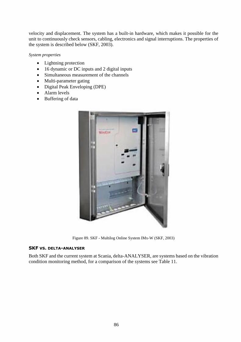
86

velocity and displacement. The system has a built-in hardware, which makes it possible for the

unit to continuously check sensors, cabling, electronics and signal interruptions. The properties of

the system is described below (SKF, 2003).

System properties

Lightning protection

16 dynamic or DC inputs and 2 digital inputs

Simultaneous measurement of the channels

Multi-parameter gating

Digital Peak Enveloping (DPE)

Alarm levels

Buffering of data

Figure 89. SKF - Multilog Online System IMx-W (SKF, 2003)

SKF VS. DELTA-ANALYSER

Both SKF and the current system at Scania, delta-ANALYSER, are systems based on the vibration

condition monitoring method, for a comparison of the systems see Table 11.

87

Table 11. SKF vs. delta-ANALYSER

Companies SKF Reilhofer

Method Vibration Vibration

System Multilog Online System

IMx-W

Delta-ANALYSER

Conversion of time-domain

data technique

FFT FFT

Number of sensors 1-2 sensors 1 sensor

Measuring channels Up to 32 channels per unit -

Training and technical

support

Yes Yes

Upgrading software cost - No

Upgrading hardware cost - Yes (Have to upgrade it every

4 years)

Cost (SEK) 115 000 SEK 500 000 SEK

Provides education Yes Yes

Help with the installation and

configuration

Yes Yes

Service and support Yes Yes

88

Possibility to use both

vibration and oil analysis

Yes Yes

3.3.3 eMaintenance Sweden AB

eMaintenance Sweden AB is a small company that have developed a decision system called

eMDSS for condition monitoring (eMaintenance, 2013).

EMDSS (E-MAINTENANCE DECISION SUPPORT SYSTEM)

eMDSS is based on new theories to improve the condition monitoring results from current

monitoring solution. This mean that the system will not replace the vibration analysis system at

Scania, instead it is used as a complement to clarify the vibration analysis results. The system is a

stand-alone system in Windows-environment, which mean that the system only is accessible by

Scania. The system cost approximately 150 000 :- (SEK).

eMDSS consist of four different tools, shown in Figure 90 and described below (eMaintenance,

2013):

PreVib (Prediction of vibration level) – Used for prediction of vibration level for a unit.

The purpose of the tool is to forecast the deviation of a unit.

ProLife (Probability of failure and remaining life) – Used for statically predict the

possibility of failure and to calculate the remaining lifetime.

AltSim (Alternative Simulations) – Makes it possible to simulate different maintenance

solutions, and choose the most cost effective solution.

MainSave (Maintenance Savings) – A tool to analyze both the technical and economical

state.

Figure 90. eMDSS (e-Maintenance Decision Support System)

89

3.3.4 Parker Hannifin

Parker Hannifin is a world leading company that offer control technologies and systems. They

provide their customers with condition monitoring systems for industrial and aerospace markets

(Parker, 2015). Parker presented two different oil particle analysis systems: icount Oil Sampler

(IOS) and Metallic Wear Debris Sensor. These systems are described in more detail below.

ICOUNT OIL SAMPLER (IOS)

Icount oil sampler is a portable condition monitoring system for measurement of particles in oil

and also fuel, see Figure 91. The application areas of the device are manufacturing, agriculture,

military and aerospace. IOS is a compact system that is both lightweight and robust, which makes

it easier to perform field analysis. The device measure particles with a laser detection particle

counter technique and it is possible to measure particles down to 4 microns and to measure the

amount of dissolved water in the oil, and the results can be downloaded onto a PC or it can be seen

on the built-in OLED display on the device (Parker, 2014). The process of the laser technique is

described in Figure 92.

Figure 91. The icountOS (IOS) particle counter (Parker, 2014)

Figure 92. The laser diode optical detection measuring process (Parker, 2014)

METALLIC WEAR DEBRIS SENSOR

The online Metallic wear debris sensor can alarm in an early stage if gears and bearings are

damaged, for the device see Figure 93. The most common application for the metallic wear debris

90

sensor is gearboxes. The advantage of the device is that it can detect both ferrous and non-ferrous

metals, which makes it blind for air-bubbles.

Figure 93. Metallic Wear Debris Sensor (Kittiwake, 2015)

The particles in the oil are detected by using an inductive coil technology, and both the amount

and size of the particles are displayed. The outputs are both digital and analogue, which means

that it easily can be integrated into existing condition monitoring systems. For an illustration of

the measuring process see Figure 94 and for the result see Figure 95.

Figure 94. Metallic Wear Debris Sensor in action (Kittiwake, 2015)

Figure 95. Number of particles (Kittiwake, 2015)

91

3.3.5 MLT

MLT (Maskin & Laserteknik AB) is a reseller of Prüftechnik, an international company. They

offer systems for vibration monitoring (MLT, 2015). MLT presented a particle counter called

Wearscanner, which is described below.

WEARSCANNER

Wearscanner is a sensor that measure the amount and size of electrically conductive particles, see

Figure 96. The particles are counted in real-time and the size is classified according to ISO 16232.

The measured data is transferred via ModBus or via online CMS (Prüftechnik, 2009).

Figure 96. Wearscanner (Prüftechnik, 2009)

The sensor using a technique based on the eddy current principal with a coil, see Figure 97, which

mean that the device works independently of oil temperature, flow rate, viscosity, air contents,

water contents and the colour of the oil. It is only possible to measure particles larger than 50 µm

and maximum measuring speed is 100 particles/second (Prüftechnik, 2009).

Figure 97. The eddy current principal (Prüftechnik, 2008)

3.3.6 ARGO HYTOS

ARGO HYTOS offer solutions for fluid power technology. They have a wide modular product

range, which makes it possible for design specialized the systems for each customer (ARGO-

HYTOS, 2014).

OPCOM FERROS

OPCom FerroS is a sensor that can determine the condition of lubrication systems, see Figure 98.

The sensor is a screw-in device, which detect ferromagnetic contamination in the lubrication. The

device has a magnet at the sensor head that record the ferromagnetic particles accumulating, and

it can distinguish between fine particles and coarse ferromagnetic fragments. The sensor has a G1”

thread and can be integrated in the gearbox. The sensor communicate over a serial RS232 interface

92

or CAN (ARGO-HYTOS, 2015). The sensor has a lot of different application areas: dump trucks,

excavator, straddle carrier, loader, milling machines, gearboxes, Forrest harvester, etc.

Figure 98. OPCom Ferros (ARGO-HYTOS, 2015)

OPCOM PARTICLE MONITOR

The OPCom Particle Monitor is a device that measure the particles in the lubrication by using

laser, see Figure 99. The device display the contamination and react quickly if the particles

increase. A digital alarm will warn when the limits have exceeded, and the readings can run time-

controlled or manually by the user. The data can be stored on an integrated memory unit during

the test, which allow recording of data over a longer period. The device has two Minimess

connections to connect the sensor (ARGO-HYTOS, 2015).

Figure 99. OPCom Particle Monitor (ARGO-HYTOS, 2015)

3.3.7 Colly Filtreringsteknik AB

Colly Filtreringsteknik AB offer their customers oil analyzing solutions, form idea to solution,

installation and service (Colly, 2015).

PCM400 CLEANLINESS MONITOR

PCM400 is a diagnostic monitoring device, which measure the cleanliness of the lubrication. For

the device see Figure 100. The device can be both be permanently installed and used as a portable

device. PCM400 use a mesh blockage technique, and the measurement results are not affected by

93

water or air. The system has a hand held touch screen programmer, which display test data in real-

time. The data are stored for trending and evaluation (Colly, 2011). The results are also graphically

reported in the trender software, see Figure 101.

Figure 100. PCM400 Cleanliness monitor and an example of a test result (Colly, 2011)

Figure 101. Trender software (Colly, 2011)

3.3.8 Comparison of the oil analysis systems

For a comparison of the oil analysis systems, see Table 12.

Table 12. Comparison of Systems

Companies Parker MLT ARGO HYTOS Colly

System

icountOS

(IOS)

Metallic

Wear

Debris

Sensor

Wearscanner

OPCom

FerroS

OPCom

Particle

Monitor

PCM400

Measuring

method

Laser

diode

Inductive

coil

Eddy

Current,

Ferro-

magnetic

sensor

Laser

diode

Proven

mesh

94

optical

detection

technolo

gy

differential

coil principle

optical

detection

blockage

technology

Fluid Flow 0,040

l/min to

0.14

l/min

1,3 l/min

to 9

l/min

1 l/min to 40

l/min

- 50 l/min to

400 l/min

-

Cost (SEK) 45 000 42 000 35 000 7 500 15 000 200 000

Upgrading

software

cost

No No - No No No

Upgrading

hardware

cost

No No - No No No

Oil

pressure

2.5 to

350 bar

0 to 20

bar

0 to 16 bar 20 bar Dynamic =

420 bar

Static = 600

bar

0 to 315

bar

Temperatu

re

+5ºC to

+80ºC

-40ºC to

+90ºC

-20ºC to

+80ºC

-40ºC to

+85 ºC

-20ºC to

+85ºC

0ºC to

+80ºC

Fluid

Viscosity

Max.

300cSt

Max.

500cSt at

40ºC

- Max.

500 cSt

- 1.5 to 450

cSt

Weight 10 kg 2.2 kg 3.5 kg 0.190 kg 0.720 kg 10.8 kg

Maintenan

ce

Maintenan

ce-free

Maintenan

ce-free

Maintenance-

free

Maintenan

ce

Maintenance -

Detection

limits

4µm-16µm

(Results

are

affected by

water or

air.)

>40

micron

Ferrous

Metal

>135

micron

Non-

Ferrous

Metal

50µm – 1000µm

(Only magnetic

particles)

4µm-

100µm

4µm - 21µm 4µm -16µm

(Every test

takes 5

minutes)

Service and

support

Yes Yes Yes Yes Yes Yes

Alarm

limits

Yes Yes Yes Yes Yes Yes

Standard ISO

4406

- ISO 16232 - ISO 4406 ISO 4406: -

/9/7 to

-/21/17

95

3.3.9 QFD – Quality Function Deployment

A QFD was made to relate customer requirements and functional requirements, and to compare

the oil analysis systems and vibration systems. As mentioned in chapter 3.2.7. oil analysis will be

used in a combination with vibration analysis, but in the QFD the oil analysis and the vibration

analysis systems have been evaluated as individual systems.

In the QFD, the upper horizontal factors are the functional requirements, while the vertical factors

are the customer requirements. The middle part of the QFD-chart is used for relating the customer-

and the functional requirements. For the QFD see Figure 102.

eMaintenance’s system called eMDSS has not been included in the QFD, because it is a decision

system, more like a software, which is applicable for the existing solution and it is not a stand-

alone system. Therefore, it was not possible to compare eMDSS with the oil analysis and vibration

systems.

Figure 102. QFD

96

Four of the highest weighted requirements are:

The system shall have a user-friendly software and hardware

The test shall stop if a damage of a bearing has reached a specific size specified by Scania

The test shall stop if a damage of a gear has reached a specific size specified by Scania

The system shall be reliable

According to the suppliers of the vibration and oil analysis system, all the systems have a user-

friendly software and hardware. The Multilog Online System IMx-W from SKF will also alarm if

a damage of a bearing or a gear has reached a specific size, but as know from using delta-

ANALYSER it can sometimes be difficult to understand the results. The oil analysis systems

cannot alarm when a specific size of a damage is reached, but the advantages of the oil analysis

system not based on laser diode optical detection, OPCom FerroS, PCM400, Metallic wear debris

sensor and Wearscanner, compared to the current system, delta-ANALYSER and STP, are their

reliability.

The systems based on laser technique, OPCom Particle Monitor and icountOS IOS, cannot

distinguish wear particles from air bubbles or water and the oil almost get whipped in the gearbox,

which results in a lot of air bubbles. Therefore, these systems are not as accurate and reliable. The

system from SKF is also accurate and reliable, according to the supplier, but it was decided to not

continue evaluating it because of lack of information. Therefore only the oil analysis systems were

further evaluated.

According to the QFD, OPCom FerroS, Metallic Wear Debris Sensor and the Wearscanner meet

the customer requirements best, see Figure 103.

Figure 103. Oil analysis systems (QFD results)

The particle detection limit differ between the systems. Therefore oil samples were sent to Exova,

providers of testing, calibration and advisory service for evaluate the cleanliness of the oil in the

gearbox during an endurance test. The oil samples were taken from the gearbox during different

times of the endurance test and sent to Exova for oil analysis. For the result of the test see Figure

104 and Figure 105. The results from Exova show that most of the particles in the oil is bigger

than 4, 6, 14 and 21 m and a little less of particles bigger than 38 and 70 m.

97

Figure 104. Oil particles distribution

Figure 105. Diagram of the oil particle distribution

Unfortunately, the systems Wearscanner and Metallic wear debris can only detect particles greater

than 50 m and 40 m, and the lab results from Exova, show that most of the particles in the oil

is greater than 4, 6, 14 and 21 m, which mean that these two systems cannot detect these particle

sizes. Therefore the OPCom FerroS sensor from ARGO HYTOS was chosen.

It will not be possible to only use oil analysis, as mentioned, therefore it was decided to continue

with a combination of current system (delta-ANALYSER and STP) and OPCom FerroS, which is

further investigated in phase 4.

3.3.10 Phase 3 – Conclusion

The third phase included demonstrations and meetings with suppliers, were the systems where

evaluated after an internal discussion. The result from the evaluation was to further investigate the

OPCom FerroS sensor system from ARGO HYTOS. Current system used by Scania was chosen

as the final vibration analysis system because SKF did not have time to demonstrate their system

during the thesis time limit. SKF only described their system.

None of the oil analysis systems found have a maximum oil temperature of 100 C, which mean

that this has to be further evaluated in phase 4.

98

3.4 Phase 4 - Detail design

A final system has been chosen and the system was evaluated in detail in phase 4. The sub-phases

for phase 4 are shown in Figure 106.

Figure 106. Phase 4 – Detail design

3.4.1 Detail design

The OPCom FerroS sensor allowas a maximum oil temperature of 85 C and the gearbox running

oil temperature is about 100 C. To solve this three different concepts of oil cooling systems for

the test-rig were developed.

CONCEPT 1

The first concept consist of a water based heat-exchanger, mounted before the oil filter on the

gearbox with quick connections. Then the flow will go through a housing including the particle

counter. The oil is filtered after passing the particle counter. The whole system is connected

together with hoses. For concept 1 see Figure 107.

Figure 107. Concept 1 – Oil flow chart

CONCEPT 2

Figure 108 show the oil temperature from an endurance test, where TV01 is the oil temperature

(heat-exchanger in) and TO01 is the oil temperature (heat-exchanger out). TV01 is approximately

99

100ºC during the test, while TO01 pedaling from approximately 82ºC to 88ºC. Therefore, it was

decided to develop a concept where the current heat-exchanger is used, instead of adding a new

one as in concept 1.

Figure 108. Oil temperature results from endurance test

The oil will flow from the gearbox, through a pressure adapter, to the heat-exchanger, then passing

the particle counter, through the filter and finally through the pressure adapter and to the gearbox,

see Figure 109. The components, pressure adapter, heat exchanger, particle counter, filter, are

connected with hoses. While the pressure adapter is mounted on the gearbox, and it has the same

interfaces and dimensions as the middle part of the filter, where the hoses are connected. The

disadvantage with this concept is that unfiltered oil is flowing through the heat-exchanger.


CONCEPT 3

Concept 3 consist of the current heat-exchanger, but the filtering device is different. The oil flow

through a pressure adapter, down to the heat-exchanger to the particle counter, then to the oil filter

100

and finally back to the gearbox. The pressure adapter consist of a bypass, which prevent too high

oil pressure for the heat-exchanger, see Figure 110. None of the current connections to the heat-

exchanger will be used. For the connections see Figure 107.


3.4.2 FMEA – Failure Mode Effect Analysis

The purpose of the Failure Mode Effect Analysis (FMEA) was to define more potential risks of

the system and recommend how these risks can be avoided. For the FMEA see Figure 111. The

oil temperature is still a risk with the final concept, because the temperature is pedaling and it can

rise to 100 C when the gearbox is unloaded.

Figure 111. FMEA

101

3.4.3 Phase 4 – Conclusion

After an internal discussion, where the concepts were discussed it was decided to choose concept

3, because of the simplicity. The only different from the current solution and concept 3 is the

pressure adapter placed between the gearbox and the middle part of the filter, which makes it easy

for Scania to develop the final solution, concept 3.

102

RESULTS

In the results chapter the results that are obtained with the methods described in the method

chapter are compiled, and analyzed and compared with the existing knowledge and theory

presented in the frame of reference chapter.

4.1 Final system

The final system is an oil contamination sensor, OPCom FerroS, from ARGO HYTOS and it will

be combined with the current system used by Scania, delta-ANALYSER and STP, see Figure 112.

A combination of oil and vibration analysis.

Figure 112. Final failure detection process

4.2 OPCom FerroS – ARGO HYTOS

OPCom FerroS is a sensor for automated condition monitoring of ferromagnetic contamination in

the lubrication, see Figure 113. OPCom FerroS is an inline system that continuously measuring

and evaluate the number of wear particles by an inductive measuring principle, and transfer is

effected via digital and analog interface. The sensor can recognize wear and damage in an early

stage, which makes it easier to distinguish the primary cause of failure. The sensor is robust against

disturbances, such as air, water and vibration.

Figure 113. OPCom FerroS (ARGO-HYTOS, 2015)

4.3 Measuring principle

The sensor determine the condition of the lubrication by recording the number of ferromagnetic

particles that stick on the magnet at the sensor head, see Figure 114. The device can distinguish

between fine particles and coarse ferromagnetic fragment, both in micrometer range and

103

millimeter range. The output signal describe the distribution of ferromagnetic particles at the

sensor surface, which is a value from 0 to 100%. The maximum amount of particles is 250 mg.

Figure 114. Measuring principal (Fredenwall, 2015)

4.3.1 Cleaning process

The sensor has an automatic cleaning process, whereupon the wear particles are released from the

sensor head. When the time interval between two cleaning processes decreases, it can be assumed

that the wear has changed, see Figure 115. The cleaning intervals can be set by the operator in the

beginning of the test.

Figure 115. Cleaning process (Fredenwall, 2015)

104

4.4 Design characteristics

The sensor has a G1 thread, and it can be integrated in the gearbox but because of the oil

temperature limit of 85 C it is not possible to integrate it in Scania’s gearboxes. Therefore, a

housing for the sensor is needed, see Figure 117. The measurements of the sensor is showed in

Figure 116.

Figure 116. Measurements (ARGO-HYTOS, 2015)

4.5 Sensor connection

A cooling oil system decrease the gearbox oil temperature when it passing the sensor. The cooling

system consist of a filter, pressure adapter, the current heat exchanger, sensor, sensor housing and

hoses, see Figure 117.

Figure 117. Oil cooling system

105

4.5.1 Flow chart

The oil flows from the gearbox to the heat-exchanger via a bypass pressure adapter, to the particle

counter, back to the pressure adapter, from the pressure adapter to the oil filter and then back to

the gearbox, see Figure 118. The pressure adapter protects the heat-exchanger pressure.

Figure 118. Flow chart

4.6 Data display and processing

A software called LubMon PClight will process and display data, and how it is working and

communicating is described further below.

4.6.1 LubMon PClight

LubMon PClight is a software that recording, storing and visualizing the incoming data from the

sensor OPCom FerroS and it is based on National Instruments’ (NI) LabView, see Figure 119. The

software can be download at ARGO HYTOS’s webpage.

Figure 119. LubMon PClight (ARGO-HYTOS, 2015)

106

COMMUNICATION

There are two different ways for the communication with the sensor: serial COM interface (RS232)

or Ethernet via TCP/IP, see Figure 120.

Figure 120. A schematic illustration of the communication between sensor and software (ARGO-HYTOS, 2015)

4.6.2 LubMon Connect

The LubMon connect is a remote gateway and will be connected with the particle sensor, OPCom

FerroS via a CANopen interface and for the device see Figure 121. During the test, the device

communicates with an internet server that store all the incoming data, and the data can directly be

visible in form of diagrams and tables. For the technical data of the LubMon Connect see Table

13.

Figure 121. LubMon Connect (ARGO-HYTOS, 2015)

Table 13. Technical data (ARGO-HYTOS, 2015)

Data Size

Temperature +5 to +50ºC

Humidity 0 to 95 % r.H.

Power supply 12 to 28 VDC

Power input Max. 0.3 A

CAN interface

Plug SUB-D9

Bus speeds 100/125/250 kBaud

107

Protocol 500 CANopen

Ethernet interface

Connection type RJ45

Speed 10/100

Protocol UDP

GSM

Aerial Stub Antenna FME

Frequencies 850 / 900 / 1800 / 1900 MHz§

4.7 Technical specification

The technical specifications for OPCom FerroS is described in Table 14.

Table 14. OPCom FerroS properties

Data Size

System OPCom FerroS

Measuring method Ferromagnetic sensor

Oil pressure 20 bar

Temperature -40 to +85 ºC

Humidity 0 to 100 % r.H.

Minimum distance to attract fine particles (1g) in lubrication with

Kinematic viscosity < 100 mm2/2 9 mm

Kinematic viscosity 300 mm2/2 7.5 mm

Kinematic viscosity 500 mm2/2 7.0 mm

Minimum flow velocity for the self-cleaning

process

0.05 m/s

Maximum flow velocity 0.1 m/s

Fluid Viscosity Max. 500 cSt

Power supply 9 to 33 VDC%

Power input Max. 0.5 A

Output

Output analog 4 to 20 mA

Accuracy of power output ± 2 %

108

Interface digital RS232/CAN

Connection

Threaded connection G1 inch

Tightening torque thread 50 ±5 Nm

Electrical Connection M12x1, 8-pole

Tightening torque M12-plug 0.1 Nm

Weight 0.190 kg

Maintenance Maintenance

Detection limits 4 to 100µm

Service and support Yes

Alarm limits Yes

Cost (SEK) 7 500

Accessories

Complete data cable set, 5 m length SCSO 100-5030

Data cable with open ends, 5 m length SCSO 100-5020

Contact box for connection of a data cable SCSO 100-5010

USB adapter – RS232 serial PPCO 100-5420

Power supply SCSO 100-5080

Ethernet – RS232 gateway SCSO 100-5100

Display and storage device LubMon Visu SCSO 900-1000

109

DISCUSSION AND CONCLUSION

In this chapter the results are discussed, the results are verified and concluded.

5.1 Discussion

The purpose of the project included two sub goals, firstly find different condition monitoring

methods and secondly choose the best solution on how to improve detection of failures.

The project resulted in a wide research of existing condition monitoring methods and solutions.

Offline testing of the oil was made with the oil analysis systems during the project, where an oil

sample of “clean oil” and oil from an already tested gearbox. The disadvantage of this method is

that the oil is filtered before analyzing. Therefore, online testing of the gearbox oil must be made

to ensure the capacity of the combination of Scania’s current system, delta-ANALYSER and STP,

and OPCom FerroS from ARGO HYTOS, which mean that the evaluation of the system

requirements in Table 15 is only based on assumptions.

Table 15. System Requirements

Row # Requirements Outcome

Per

form

an

ce

1 The system shall be easy to access in the test-rig, 10 min

2 The system shall be easy to maintain and service

3 The system shall have a user-friendly software and hardware

4 The system shall provide the user with accurate result

5 The system should provide the user with automated data

acquisition

6 The system shall be reliable

7 The system shall provide the user with automated data

management and trending

8 The system shall be flexible

9 No expertise shall be needed to operate the system

10 The system shall be alert and alarm if a limit is reached.

11 The system shall have a data storage

12 The system shall be user-friendly to operate

13 The system shall have automatic trending

14 The system shall be able to handle high temperatures (oil

temperature = 100°C)

15 The system shall simplify diagnostic of the gearbox

110

Com

pan

y c

on

stra

ints

16 The test shall stop if a damage of a bearing has reached a specific

size specified by Scania

17 The test shall stop if a damage of a gear has reached a specific

size specified by Scania

18 The system shall be able to use for all the different types of

gearboxes at Scania

19 The gearbox must be unaffected in terms of function and strength

Main

ten

an

ce

20 The system shall provide the user with easy access to the parts

that require maintenance, less than an hour

21 No need for special tools

Syst

em

Lif

e S

pan

22

The system shall be in production for 10 years

Safe

ty

23 The system shall protect the safety of the employees

24 No heavy lifting > 8 kg

Inst

all

ati

on

25 Installation Instructions

26 Scania standards for the components (TFP - Technical

regulations for machinery production equipment) - 2011-12-29

Docu

men

tati

on

27 Training and technical support shall be provided

28 Operation instructions shall be provided

29 Instruction on how to disassembly the system shall be provided

30 Instructions on how to recycle the parts shall be provided

31 The system shall provide the user with an automatic report

Cost

32 Operating cost

33 System cost

Oil and vibration analysis are natural partners when condition monitoring machines. Combination

of these two systems enables control of balance alignment and looseness. The oil analysis system,

OPCom FerroS, will enable control over the lubricant quality and contamination. The advantage

with both systems is that the strength of vibration analysis counteract the limitation of the oil

analysis and vice versa, to ensure the health of the gearbox. A gearbox is complex, so two different

solutions will make the result more reliable. The contaminations will weaken the lubrication

strength. Other risks are misalignment, unbalance and looseness. These failures will shorten the

life of a gearbox.

111

The oil analysis system can early detect contamination in the oil, a component is probably damaged

if delta-ANALYSER and STP also indicates a failure. An early warning from the analysis systems

will make it easier to determine the root cause of a failure.

Detecting wear-related faults can be challenging, because of background noise, especially at slow

speed where the amplitude of the vibration signal is not strong enough. Therefore oil analysis is a

good complement, it can early detect contact fatigue, abrasion and adhesive wear. The

disadvantage is that oil analysis cannot distinguish the location of the failure, this will be possible

with vibration analysis. Unfortunately, delta-ANALYSER cannot exactly locate the source of the

defect because of overlapping orders. Another disadvantage with the final solution is that it cannot

alarm if a damage of a component has reached a specific size, see requirements 16-18 in Table 15.

This has to be further investigated, but together vibration and oil analysis will make a good

combination for early detection of failures in the gearbox.

5.2 Conclusion

The chosen method was structured, detailed and well planned for this project. It created a natural

flow in the work process, and it was easy to follow the method through the whole project. The

modification of the CPS process was suitable for the thesis work, and having decided the tools and

methods in the beginning brought the project forward. Unfortunately, working too long with each

phase was a problem and also the summer holiday of the employees at Scania and suppliers of the

systems. Therefore, the Gantt chart should have been more detailed and the summer holiday should

have been taken in account when making the schedule.

The thesis work resulted in a combination of two systems: Scania’s current solution, delta-

ANALYSER and STP, and OPCom FerroS oil particle sensor from ARGO HYTOS. The purpose

of the thesis work can be considered fulfilled since an investigation of existing condition

monitoring methods were accomplished and after internal discussions, where methods and tools

were conducted, the most appropriate system was chosen. If the final system improve detecting of

failures has to be tested.

The delimitations made in the beginning of the project, was not concrete enough. These should

have been more detailed, because it was difficult to distinguish the scope of the project, but the

detailed methodology made it easier to accomplish a good flow of the project process.

It is assumed that the final system will meet 22 of the 33 requirements, but this has to be tested.

The final system still consist of delta-ANALYSER, which mean that the hardware and software

will not be user-friendly, even if the OPCom FerroS has it. Therefore, some expertise will be

needed to use the final combination of systems. It is impossible to say if the result will meet the

company constraints, because it has to be tested. The final result will become more expensive,

because the current systems used by Scania will be kept.

There have been some limitations during the project, such as the summer holiday which shorten

the planned time of demonstrations, and it would have been interesting to compare the vibration

system from SKF with delta-ANALYSER, but there was not enough time. There have not been

any in-depth development of the final cooling oil system, because of the time limitation.

112

FUTURE WORK

In this chapter the recommendations and suggestions for future work to improve the detection of

failures are presented.

6.1 Future work

It is recommended that the final combination of systems is tested in the test-rig and further

investigated. The maximum temperature of the sensor is 85C and with the developed oil cooling

system the temperature range is approximately 82ºC to 88ºC, and sometimes the temperature can

rise to 100 C. The oil cooling system described in the report is only a sketch of the system, and

this has to be evaluated further. In the final oil cooling system the oil will not be filtered before it

goes through the heat-exchanger, which can affect it, and also evaluate if the oil pressure will

decrease, because it must should be around 2.3 and 2.8 bar. Another solution would be to continue

to search and try to find an oil analysis sensor that has a maximum temperature of 100 ºC.

Maybe adding a sensor from ARGO HYTOS, called LubCos H20plus II, which can measure the

conductivity and the permittivity in the oil to improve the condition of the oil. This sensor can be

place next to the OPCom FerroS sensor, see Figure 117.

The delta-ANALYSER is not accurate enough, and it would therefore be a good idea to further

investigate delta-ANALYSER and maybe the amount of sensors. Today Scania is using one

sensor, which mean that the sound has to travel a long way before it is collected. It would be good

to analyze if adding more sensors would improve the results.

Investigate a new vibration system, such as Multilog Online System IMx-W from SKF, would also

be a good idea or continue with the eMaintenance project and investigate if the their system can

improve the results from STP. If eMaintenance’s decision system is working as good as the

company says, then Scania can stop using delta-ANALYSER and only use STP. One of the

disadvantages with delta-ANALYSER is that the company is located in Germany, which makes it

more difficult for the company to check the system if Scania have any problems, while both

eMaintenance and SKF is located in Sweden.

113

REFERENCES

ABB, 2014. Condition Monitoring. [Online]

Available at: http://new.abb.com/power-generation/instrumentation/Condition-

Monitoring

[Använd 26 06 2015].

Abernethy, R. B., Breneman, J. E., Medin, C. H. & Reinman, G., 1983. Weibull Analysis

Handbook. Florida: Pratt & Whitney Aircraft.

Ai, S. & Hui Li, L. F., 2009. Gear Fault Diagnosis Based on EMD and AR Spectrum Analysis.

International Conference on Measuring Technology and Mechatronics Automation,

Volume 1, pp. 673-676.

Al-Badour, F., Sunar, M. & Cheded, L., 2011. Vibration analysis of rotating machinery using

time-frequency analysis and wavelet techniques. Mechanical Systems and Signal

Processing, 25(6), pp. 2083-2101.

Almkvist, A. L., 2015. Acoustic emission methods in fatigue testing, Stockholm: KTH Industrial

Engineering and Management.

Anjar, B., Dalberg, M. & Uppsäll, M., 2011. Feasibility study of thermal condition monitoring

and condition based maintenance in wind turbines, Kalmar: Elforsk.

ARGO-HYTOS, 2014. About us. [Online]

Available at: http://www.argo-hytos.com/company/about-us.html

[Använd 26 06 2015].

ARGO-HYTOS, 2015. LubMon PClight. [Online]

Available at: http://www.argo-hytos.com/products/sensors-

measurement/software/lubmon-pclight.html

[Använd 24 08 2015].

ARGO-HYTOS, 2015. LucMon Connect. [Online]

Available at: http://www.argo-hytos.com/products/sensors-measurement/data-

handling/lubmon-connect.html

[Använd 20 08 2015].

ARGO-HYTOS, 2015. OPCom Particle Monitor. [Online]

Available at: http://www.argo-hytos.com/products/sensors-measurement/stationary-

particle-monitor/opcom-particle-monitor.html

[Använd 10 08 2015].

ARGO-HYTOS, 2015. Wear Sensor - OPCom FerroS. [Online]

Available at: http://www.argo-hytos.com/products/sensors-measurement/stationary-

particle-monitor/opcom-ferros.html

[Använd 14 08 2015].

114

Askalon, 2014. Condition based maintenance with AMS suite. [Online]

Available at: http://www.askalon.com/en/businessarea/AssetManagement

[Använd 26 06 2015].

Bedmar, A. P., 2013. Synchronization processes and synchronizer mechanisms in manual

transmission, Göterborg: Department of Applied Mechanics, Chalmer University of

Technology.

Bindt, 2013. Acoustic Emission. [Online]

Available at: http://www.bindt.org/What-is-NDT/Acoustic-emission-AE/

[Accessed 23 04 2015].

Bogue, R., 2013. Sensors for condition monitoring: a review of technologie and applications.

Sensor Review, 33(4), pp. 295-299.

Brian, M., 2012. “How Manual Transmission work”. [Online]

Available at: http://auto.howstuffworks.com/transmission2.htm.

[Accessed 16 04 2015].

CJC, 2015. Clean Oil Guide, Svendborg: C.C.JENSEN A/S.

Colly, 2011. Pall PCM400 Series fluid cleanliness monitor, u.o.: Pall corporation.

Colly, 2015. Om oss. [Online]

Available at: http://www.collyfiltreringsteknik.se/om-oss/

[Använd 10 08 2015].

CREO, 2014. About Us. [Online]

Available at: http://www.creodynamics.com/home/about-creo-dynamics

[Använd 26 06 2015].

Dahunsi, O., 2008. Spectrometric Oil Analysis - An Untrapped Resource for Condition

Monitoring. Research gate, 12(2), pp. 107-114.

Davies, A., 1998. Handbook of condition monitoring: techniques and methodology. 1st red.

u.o.:Chapman & Hall.

Dekra, 2014. Non-Destructive Testing - NDT. [Online]

Available at: http://www.dekra-industrial.se/en/tjanster/non-destructive-testing-ndt

[Använd 26 06 2015].

Denghua, L., Xiangyu, G., Feng, Z. & Zhixin, Z., 2010. Research on nonlinearity property of

piezoelectric vibration accelerometer based on cymbal transducer. International

conference on information and automation, pp. 930-934.

DeVries, D., 2013. Crack Testing and Heat Treat Verification of Gears Using Eddy Current

Technology. American Gear Manufacturers Association, pp. 50-55.

115

DISCOM, 2012. Products for acoustic quality analysis. [Online]

Available at: http://www.discom.de/DiscomWebSite/en/ProductOverview.htm

[Använd 26 06 2015].

Discom, 2012. Rotas Noise Analysis System - Manual and Introduction, Göttingen: Discom

Industrial Measurement and Test Systems.

Einarsson, H., 2011. Bruksanvisning för Scania provcell T17 - STP Styrsystem, Södertälje:

Scania.

eMaintenance, 2013. eMDSS - besultssystemet för att omvandla förlust till vinst. [Online]

Available at: http://www.e-maintenance.se/?page_id=892

[Använd 10 08 2015].

Felten, D., 2003. Understanding bearing vibration frequencies, Wiconsin: L&S Electric, Inc.

Flexolan, 2015. Structure-borne sound and airborne sound. [Online]

Available at: http://www.flexolan.com/cms/lng/en/structure-borne-sound-and-airborne-

sound.html

[Accessed April 2015].

FLIR, 2015. Vårt Företag. [Online]

Available at: http://www.flir.se/cs/display/?id=41529

[Använd 26 06 2015].

Fluke, 2014. Produkter. [Online]

Available at: http://www.fluke.com/fluke/sesv/products/default.htm

[Använd 26 06 2015].

Forsthoffer, W. E., 2011. Forsthoffer's best practice handbook for rotating machinery. 1st red.

u.o.:Elsevier.

Fredenwall, L., 2015. Oil Condition Monitoring with sensors in the hydraulic fluid. Södertälje:

ARGO HYTOS.

Ganeriwala, S., 2010. Review of techniques for bearings and gearbox diagnostics. Richmond:

SpectraQuest, Inc.

Gantt, 2015. What is a Gantt chart?. [Online]

Available at: http://www.gantt.com/

[Använd 28 07 2015].

Gatti, P. L., 2003. Applied Structural and Mechanical Vibrations: Theory Methods ans

Measuring Instrumentation. 1st red. London: E & FN Spon.

Gebarin, S., 2003. Machinery Lubrication. [Online]

Available at: http://www.machinerylubrication.com/Read/521/in-line-wear-debris-

detectors

[Använd 08 07 2015].

116

Graney, B. P. & Starry, K., 2011. Rolling element bearing analysis. The american society for

nondestructive testing, 70(1), pp. 78-85.

Grünbaum, A. F., 1992. Ten Lectures on Wavelets. Science, 257(5071), pp. 821-822.

Gupta, A. & Karma, V., 2014. Fault analysis of two stage gearbox using acoustic emission

signal: Effect of spalling. International journal of engineering sciences & research

technology, 7(3), pp. 716-721.

Gustavsson, G., 2006. Bruksanvisning för Scania provcell T17, Södertälje: Scania.

Head-acoustics, 2015. Vehicle Acoustic - Powertrain NVH - Structure-Borne Sound Transfer.

[Online]

Available at: https://www.head-

acoustics.de/eng/nvh_consulting_automotive_applications_powertrain_structure-

borne.htm

[Använd 14 04 2015].

Hellier, C., 2003. Handbook of Nondestructive Evaluation. 1st red. New York: McGraw-Hill.

Holloway, M. & Nwaoha, C., 2013. Dictionary of Industrial Terms. s.l.:John Wiley & Sons, Inc.

Huang, N. E. o.a., 1998. The empirical mode decomposition and the Hilbert spectrum for

nonlinear and non-stationary time series analysis. Proceedings of the Royal Society:

Mathematical, Physical and Engineering Science, 454(1971), pp. 903-995.

Hydac, 2015. Products. [Online]

Available at: http://www.hydac.com/uk-en/start.html

[Använd 26 06 2015].

Jaffard, S., Meyer, Y. & Ryan, R. D., 2001. Wavelets: Tools for Science & Technology. 1st red.

Philadelphia: Society for Industrial and Applied Mathematics.

Kaplan, B. & Duchon, D., 1988. Combining Qualitative and Quantitative Methods in

Information SYstems Research: A Case Study. Management Information Systems

Research Center, 12(4), pp. 571-586.

Karlsson, J., 2015. Course - Transmission. Södertälje: Scania.

Kittiwake, 2015. On-Line Metallic Wear Debris Sensor. [Online]

Available at: http://www.kittiwake.com/metallic-wear-debris-sensor

[Använd 02 07 2015].

Laboratories, M., 2003. Direct Read Ferrograph. [Online]

Available at: http://www.mrtlaboratories.com/direct_read_ferrography.htm

[Använd 09 06 2015].

Li, H., Zheng, H. & Tang, L., 2005. Hilbert-Huang transform and its application in gear faults

diagnosis. Key Engineering Materials, Volume 291-292, pp. 655-660.

117

Li, H., Zheng, H. & Tang, L., 2010. Gear Fault Detection Based on Teager-Huang Transform.

International Journal of Rotating Machinery, Volume 2010, pp. 1-9.

Lindholm, G., 1995. Vibrationer i maskiner, Del 6 av 10 (Vibrationsorsaker). 1st red.

Norrköping: Mentor Communications AB.

Lovicz, R. & Dalley, R., 2005. Wear Particle Analysis - A Predictive Maintenance Tool.

[Online]

Available at: http://www.reliabilityweb.com/art05/wear_particle-analysis.htm

[Använd 09 06 2015].

Lubrication, M., 2002. The Low-Down on Particle Counters. [Online]

Available at: http://www.machinerylubrication.com/Read/351/particle-counters

[Använd 15 06 2015].

Ludeca, 2011. Machinery fault diagnosis. u.o.: Prüftechnik.

Mastro, M., 2013. Financial Derivative and Energy Market Valuation: Theory and

Implementation in Matlab. 1st ed. s.l.:John Wiley & Sons.

MaterialScience2000, 2014. Magnetic particle inspection. [Online]

Available at: https://www.youtube.com/watch?v=qpgcD5k1494

[Använd 28 07 2015].

MaterialsScience2000, 2014. Ultrasonic Testing. [Online]

Available at: https://www.youtube.com/watch?v=UM6XKvXWVFA

[Använd 27 07 2015].

Mistras, 2014. Mistras Products & System Division. [Online]

Available at: http://www.mistrasgroup.com/products/

[Använd 26 06 2015].

MLT, 2015. Produkter från MLT. [Online]

Available at: http://www.mlt.se/produkter

[Använd 26 06 2015].

Mobley, K. R., 2001. Plant Engineer's Handbook. 1st red. Woburn: Butterworth-Heinemann.

Mobley, K. R., 2001. Vibration Fundamentals. s.l.:Elsevier.

Mobley, K. R., 2002. Introduction to predictive maintenance. 2nd ed. Woburn: Elsevier Science.

Mohanty, A. R., 2015. Machinery Condition Monitoring. In: New York: Taylor and Francis

Group, pp. 1-17.

MTS, 2014. Fluid Assessment. [Online]

Available at: https://www.mts.com/en/services/maintain/fluid-assessment/index.htm

[Använd 26 06 2015].

118

Newport, 2015. Vibration Control. [Online]

Available at: http://www.newport.com/Unit-Conversion-Charts-and-Constants-Vibration-

Co/168093/1033/content.aspx

[Använd 15 11 2015].

NORELLS, 2007. Termografi. [Online]

Available at: http://www.termografi.se/termografi.html

[Använd 26 06 2015].

Noria, 2002. Particle Counting - Oil analysis 101. [Online]

Available at: http://www.machinerylubrication.com/Read/353/particle-counting-oil-

analysis

[Använd 27 07 2015].

Noria, 2012. How important is the ISO cleanliness code in oil analysis?. [Online]

Available at: http://www.machinerylubrication.com/Read/28979/iso-cleanliness-code

[Använd 27 07 2015].

Olsson, C., 1997. Utmattning av lastbilskomponenter, Södertälje: Scania.

Olsson, C., 1997. Utmattning av lastbilskomponenter, Södertälje: Scania.

Parker, 2014. icount Oil Sampler (IOS), u.o.: Parker Hannifi.

Parker, 2015. About us. [Online]

Available at:

http://www.parker.com/portal/site/PARKER/menuitem.f830ba32f37af5fe2c5c8810427ad

1ca/?vgnextoid=7de94bad565e4310VgnVCM10000014a71dacRCRD&vgnextfmt=defau

lt

[Använd 26 06 2015].

PCB, 2015. Introduction to Piezoelectric Accelerometers. [Online]

Available at: https://www.pcb.com/techsupport/tech_accel.aspx

[Använd 12 05 2015].

Peng, Z. & T.B, K., 1999. Wear particle classification in fuzzy grey system. Wear, Volym 225,

pp. 1238-1247.

phmsociety, 2009. Domain Fundamentals. [Online]

Available at: http://www.phmsociety.org/competition/PHM/09/fundamentals

[Accessed 29 04 2015].

Picotech, 2014. PT100 platinum resistance thermometers. [Online]

Available at: https://www.picotech.com/library/application-note/pt100-platinum-

resistance-thermometers

[Accessed 17 04 2015].

Polak, S., 1999. Gearbox and Gear System problems. [Online]

Available at: http://tribology.co.uk/publish/p004.htm

[Använd 10 07 2015].

119

Prüftechnik, 2008. Wearscanner - Online particle distribution counter monitors wear debris in

oil, Ismaning: Prüftechnik.

Prüftechnik, 2009. Wearscanner, Ismaning: Prüftechnik.

Prytz, U., 2008. Konceptbeskrivning T17, Södertälje: Scania.

Puccio, G. et al., 2011. The CPS Process. [Online]

Available at: http://www.creativeeducationfoundation.org/creative-problem-solving/the-

cps-process/

[Accessed 27 04 2015].

Randall, R. B., 2010. Vibration-based condition monitoring: industrial, aerospace and

automotive applications. 1st ed. United Kingdom: John Wiley & Sons.

Rasmussen, C. E. & Williams, C. K., 2006. Gaussian Processes for Machine Learning. In: T.

Dietterich, ed. London: MIT press, pp. 1-2.

Reilhofer, 2014. Delta Analyser v2 - Manual, München: Reilhofer.

Ringholm, E., 2004. Understanding filter beta ratios. [Online]

Available at: http://www.machinerylubrication.com/Read/564/filter-beta-ratios

[Använd 06 08 2015].

Rohloff, 2015. Planetary Gear System. [Online]

Available at: http://www.rohloff.de/en/technology/speedhub/planetary_gear_system/

[Accessed 06 05 2015].

Saeed, A., 2008. Online Condition Monitoring System for Wind Turbine, Blekinge: Blekinge

Institute of Technology.

Scania, 2011. Pressroom: New global engine range. [Online]

Available at:

http://www.scania.com/%28S%28lv3lzx55wgsfyzzfdjz32v55%29%29/media/calendar/2

011/pressroom-new-global-scania-engine-range/index.aspx?tab=5

[Använd 25 06 2015].

Scania, 2012. CombaT Basic. [Online]

Available at: http://combat.scania.com/basic/

[Accessed 16 04 2015].

Scania, 2015. 05-00 GRS905, Södertälje: Scania.

Scania, 2015. Scania Image Archive. [Online]

Available at:

https://scaniaimagearchive.scania.com/fotoweb/Grid.fwx?position=9&archiveId=5010&c

olumns=4&rows=2&sorting=ModifiedTimeAsc&search=(IPTC020%20contains(Compo

nents%20and%20Powertrain%20and%20Gearbox))

[Använd 16 06 2015].

120

Shen, S. S. & Huang, N. E., 2005. Hilbert-Huang Transform and Its Applications. s.l.:s.n.

Shipley, E. E., 1967. Gear Failures. Co., Cleveland, Ohio, p. 12.

Shull, P. J., 2002. Nondestructive Evaluation: Theory, Techniques and Applications. 1st red.

u.o.:Marcel Dekker.

Singh, A., Houser, D. R. & Vijayakar, S., 1999. Detecting Gear Tooth Breakage Using Acoustic

Emission: a Feasibility and Sensor Placement Study. Journal of Mechanical Design,

Volume 121, pp. 587-593.

SKF, 1994. Bearing failures and their causes, Sverige: Palmeblads Tryckeri AB.

SKF, 2003. SKF Multilog On-line system IMx-W, Luleå: SKF.

SKF, 2015. Om oss. [Online]

Available at: http://www.skf.com/se/our-company/index.html

[Använd 26 06 2015].

Sun, C.-L.o.a., 2006. High sensitivity cymbal-based accelerometer. Scientific instruments, 77(3),

pp. 1-3.

Sun, H. o.a., 2014. Multiwavelet transform and its applications in mechanical fault diagnosis - A

review. Mechanical Systems and Signal Processing , 43(1-2), pp. 1-24.

Supervision, 2014. Thermal Imaging. [Online]

Available at: http://www.supervision.co.nz/wp-content/uploads/Gearbox.jpg

[Använd 28 07 2015].

Torrington, T., 2000. Bearing failures prevention guide, s.l.: Ingersoll-Rand.

TWI, 2015. Radiography Testing. [Online]

Available at: http://www.twi-global.com/capabilities/integrity-management/non-

destructive-testing/ndt-techniques/radiography-testing/

[Använd 28 07 2015].

Ullman, D., 2010. The mechanical design process. 4 red. Boston: McGraw-Hill.

Ulrich, K. & Eppinger, S., 2012. Product Design and Development. 5 red. Boston: McGraw-

Hill/Irwin.

Vibrationschool, 2015. Rolling element bearings. [Online]

Available at: http://www.vibrationschool.com/mans/SpecInter/SpecInter24.htm

[Använd 17 07 2015].

Weibull, 2015. Life Data Analysis (Weibull Analysis). [Online]

Available at: http://www.weibull.com/basics/lifedata.htm

[Accessed 22 04 2015].

121

Williamson, M., 2009. Mesh blockage particle monitoring. [Online]

Available at: http://www.machinerylubrication.com/Read/2018/mesh-blockage

[Använd 27 07 2015].

Appendix A. Page 1(1)

1

APPENDIX A: Thesaurus

Abrasive Wear: The wear between two surfaces in relative motion, and the reason for this type

of wear can be particles (three bodies) or surface roughness (two bodies) (Holloway & Nwaoha,

2013, p. 3).

Acceleration: When the velocity of a body or particle change with respect to the time (Holloway

& Nwaoha, 2013, p. 6).

Accelerometers: A device used for measuring the acceleration. The parameter measured by the

accelerometer is 𝑑𝑣/𝑑𝑡 (Holloway & Nwaoha, 2013, p. 7).

Amplitude: The amplitude is a measurement of the distance from the highest to the lowest

excursion of motion, e.g. a mechanical body in oscillation or for an electrical waveform, it can be

the peak-to-peak swing (Holloway & Nwaoha, 2013, p. 32).

Debris: Particles

Fast Fourier Transform (FFT): A method used to convert time based spectra to frequency based.

Frequency: The number repeating events occur per unit time (Holloway & Nwaoha, 2013, p.

265).

Gaussian Process: In a Gaussian process every point in space is associated with a normally

distributed random variable, which means that a finite dimensional distribution has a multivariate

normal distribution, a generalization of the one-dimensional normal distribution to dimensions that

are higher (Rasmussen & Williams, 2006).

Stress: Stress is like an internal force field within a structure, and it is the stress that transmit and

balance the external load (Shull, 2002, p. 536).

Planetary transmission system: A planetary gear system consists of a sun gear in the center, a

ring gear and also several planet gears which rotate between these (Rohloff, 2015).

Piezoelectric sensor: It is an optical or inductive sensor which determines the corresponding

rotation speed (Reilhofer, 2014).

Vibration: It is a mechanical phenomenon, and it happens when oscillations occur about an

equilibrium point. Then the vibration transducer, a sensor, converts this movement into an

electrical signal (Holloway & Nwaoha, 2013, p. 647).

Appendix B. Page 1(1)

2

APPENDIX B: Risk-analysis

Appendix C. Page 1(1)

3

APPENDIX C: Interviewees

Appendix D. Page 1(1)

4

APPENDIX D: Persona

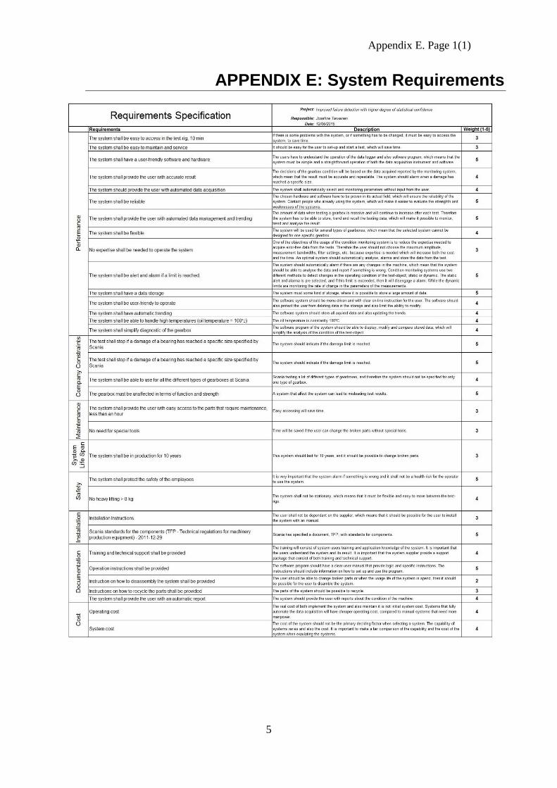
Appendix E. Page 1(1)

5

APPENDIX E: System Requirements

improved failure detection with higher degree of

Documents