improved energy modelling of wireless personal area network
TRANSCRIPT

Improved Energy Modelling of Wireless Personal Area Network
1
Technical Report, IDE 0945, May 2009
Improved Energy Modelling of Wireless Personal Area Network
Master’s thesis in Computer System / Electrical Engineering
Junaid Wahab and Zubair Ali
Supervisors
Nicholas Wickström
Wagner de Morais
_______________________________________________________________________
_______________________________________________________________________
School of information sciences, Computer and Electrical Engineering Halmtad University

Improved Energy Modelling of Wireless Personal Area Network
2

Improved Energy Modelling of Wireless Personal Area Network
3
Title
Master’s thesis in Computer System / Electrical Engineering
School of Information Science, Computer and Electrical Engineering Halmstad University
Box 823, S-301 18 Halmstad, Sweden
May, 2009

Improved Energy Modelling of Wireless Personal Area Network
4

Improved Energy Modelling of Wireless Personal Area Network
5
Preface In the name of the Lord, “ALLAH”, who is our GOD.
Taking advantage of this opportunity I pay my sincere gratitude to my family for there help
and support thought-out my stay in Sweden. I would like to say special thanks to my elder
brother and younger sister for there continuous encouragement.
I do want to mention that due to the technical support of my supervisors especially Wagner de
Morais, made it possible to achieve this milestone.
At the end I would like to thank my friend Mirza Aamir Mehmood for his kind advices during
the span of this thesis.
Zubair Ali Taking advantage of this opportunity I pay my sincere gratitude to my family for there help
and support thought-out my stay in Sweden. I would like to extend my gratitude to our
supervisors for there technical support and encouragement.
Junaid Wahab Halmstad University, May 2009

Improved Energy Modelling of Wireless Personal Area Network
6

Improved Energy Modelling of Wireless Personal Area Network
7
Abstract Wireless sensors networks are used in a variety of environments ranging from environment
monitoring such as humidity and temperature, to environments like patient monitoring, habitat
monitoring etc. Sometimes sensors are deployed in inaccessible or hazardous places, and they
are battery operated; recharging or changing the sensor’s battery is almost impossible.
In such scenarios, where the battery can not be recharged or changed, it is crucial to know in
advance how long the battery will last so that the old sensor node can be replaced by a new
one. Normally, in order to effectively utilize the battery the components of a wireless sensor
node are turned off when not needed.
This paper presents an in-depth analysis of the importance of switching sensor node
components, and its impact on the life time prediction. A new energy model is presented
which caters for the current and time consumed in switching from one mode to another. A
comparison is made between scenarios where current consumption while switching is catered
with the one where it is not catered. This was achieved by using on chip fuel gauge, with
some limitation, which was verified by using digital multimeter.

Improved Energy Modelling of Wireless Personal Area Network
8

Improved Energy Modelling of Wireless Personal Area Network
9
Table of contents
1. Introduction ...................................................................................................................... 13
1.1. Goal .......................................................................................................................... 13
1.2. Limitation ................................................................................................................. 14
2. Background ...................................................................................................................... 17
2.1. Wireless sensor network........................................................................................... 17
2.2. Hardware Components ............................................................................................. 17
2.2.1. Power Source........................................................................................................ 18
2.3. Software Components .............................................................................................. 18
2.3.1. Operating Systems................................................................................................ 18
2.3.2. TinyOS ................................................................................................................. 19
2.3.3. Middleware........................................................................................................... 19
2.4. Power Consumption in Wireless Sensor Node ........................................................19
3. Related Work.................................................................................................................... 23
3.1. Power Management in Embedded System............................................................... 23
3.2. Event Driven Approach............................................................................................ 23
3.3. Power Management in Embedded Medical System................................................. 24
3.4. Power management in wireless sensor network....................................................... 25
3.5. An Application-driven Approach............................................................................. 25
3.6. Middle ware for Distributed Sensor Environment...................................................26
4. Proposed Implementation................................................................................................. 29
4.1. Dynamic Energy Modeling Scheme ........................................................................ 29
4.2. System modes........................................................................................................... 29
4.2.1. Low Power Mode ................................................................................................. 29
4.2.2. Sensing Mode....................................................................................................... 30
4.2.3. Communication Mode.......................................................................................... 30
4.2.4. Full Power Mode.................................................................................................. 30
5. Methodology .................................................................................................................... 33
5.1. Hardware .................................................................................................................. 33
5.1.1. Microchip PIC18F25K20 Flash Microcontroller ................................................. 34
5.1.2. VTI Technologies SCA3000-E04 3-Axis Ultra low Power Accelerometer ........ 34
5.1.3. Free2move Low power Audio Bluetooth™ Module with antenna F2M03ALA. 35
5.1.4. Maxim DS2756 High-Accuracy Battery Fuel Gauge .......................................... 36
5.1.5. Battery .................................................................................................................. 36
Improved Energy Modelling of Wireless Personal Area Network
10
5.2. Software ................................................................................................................... 36
5.2.1. MPLAB IDE ........................................................................................................ 36
5.2.2. MPLAB ICD 2 ..................................................................................................... 37
5.2.3. BoostC Compiler.................................................................................................. 37
5.3. Implementation......................................................................................................... 37
5.3.1. Experimental Setup .............................................................................................. 37
5.4. Node Level Current Consumption ........................................................................... 40
5.4.1. Measurement through Agilent 34410 A 6 ½ Digit Multimeter............................ 40
5.4.2. Measurement through DS2756 fuel gauge........................................................... 47
5.5. Model level Current Consumption........................................................................... 49
5.5.1. Low Power Mode – Sensing ................................................................................ 50
5.5.2. Sensing ................................................................................................................. 51
5.5.3. Communication .................................................................................................... 51
5.5.4. Low Power Mode – Communication ................................................................... 51
6. Summary .......................................................................................................................... 55
6.1. Better Life Time Prediction...................................................................................... 55
6.2. Better Threshold Prediction ..................................................................................... 55
7. Discussion ........................................................................................................................ 57
8. Conclusion........................................................................................................................ 59
9. References ........................................................................................................................ 61

Improved Energy Modelling of Wireless Personal Area Network
11
List of Figures
Figure 1: Block diagram of a sensor node................................................................................ 17
Figure 2: Tranzition from one system sate to another ............................................................ 21
Figure 3: Sensor states of a power-aware node........................................................................ 27
Figure 4: States of sensor node. ............................................................................................... 31
Figure 5: Body area sensor node with battery.......................................................................... 34
Figure 6: Microchip PIC18F25K20 flash microcontroller....................................................... 34
Figure 7: VTI Technologies SCA3000-E04 3-Axis accelerometer ......................................... 35
Figure 8: Audio Bluetooth™ module with antenna F2M03ALA ............................................ 35
Figure 9: Bluetooth™ Serial Port Plug - F2M01C1................................................................. 38
Figure 10: Flow chart. .............................................................................................................. 39
Figure 11: PIC in differnt Fequencies ...................................................................................... 41
Figure 12: Shows the current and time consumed while transitioning from sleep to active ... 42
Figure 13: Current consumed and time spend while sensing hundred samples....................... 43
Figure 14: Current consumption of the sensor node while Bluetooth module is turned on..... 44
Figure 15: Current consumed and time taken by the sensor node in connecting and. ............. 45
Figure 16: Current consumed by the sensor node while Bluetooth module is kept on............ 46
Figure 17: Current consumption by sensor node while in Low power mode to. ..................... 50
Figure 18: Current consumption while the sensor node is in LMP, Communication. ............. 52
Figure 19: Life time prediction ................................................................................................ 56

Improved Energy Modelling of Wireless Personal Area Network
12
Improved Energy Modelling of Wireless Personal Area Network
13
1. Introduction
Moore's law describes a central drift in the electronic hardware where the number of
transistors that can be placed on an electronic circuit doubles approximately every two years.
This trend has continued now for more than half a century. Different aspects of electronic
devices, like processing, memory and functionality like the resolution of digital cameras are
improved at exponential rates. Similarly, the size of wireless sensor nodes is getting smaller
and they are becoming much more efficient. Wireless sensor nodes can be powered either
with wired power cables or with batteries but, in some situations, it may not be physically
possible or desirable to change or recharge these batteries. An obvious solution to this is to
use batteries with more charge but, unfortunately, the size of the battery is directly
proportional to the charge. This means that more the battery capacity the bigger the battery,
due to which the full advantage of minimization may not be taken.
Power in sensor nodes is used for sensing, computing, and communicating. Modern sensor
nodes try to shut down these components or, regulate processing frequency, whenever
possible to save power, though the energy utilization rate for every type of process is sensor
and function specific. Research has shown that a sensor node's energy utilization for
communication activities exceeds that necessary for sensing and computation. Dropping
communication frequency was one method used to preserve energy.
The sensor node is composed mainly of four, high-level components, namely microprocessor,
sensor, communication module and power supply. The sensor, communication module and
microprocessor can be in different modes, with different energy consumptions. The sensor
and communication components can switch between ACTIVE, SLEEP and OFF modes.
Different techniques can be used to save power. One of them is dynamic power management.
Switching between different modes can be dynamically managed by the power manager [6].
1.1. Goal
In the past, different approaches have been followed to make a sensor node power
efficient. The radio is the most power consuming component in a wireless sensor network.
One straight forward answer to this is to turn on the radio to transmit or receive, and then turn
it off.

Improved Energy Modelling of Wireless Personal Area Network
14
Components such as the microcontroller, and the sensor itself, can not be disregarded; they
can also be used in a similar fashion in order to reduce the power consumption, but this
approach can be the cause of more power consumption in some cases. If it takes more power
to turn off and on these components, and it is more efficient to keep these components on all
the time. Another important aspect of this is the time taken to change the mode of these
components. One more thing that needs to be considered is that, if it is desired to have a
sensor with sampling rate of 10 Hz but in order to change the state of the sensor to sleep and
then back to active, it takes 110 milliseconds, and then the requirements of sampling at the
desired rate cannot be fulfilled if the sensor changes its state.
In this research, how the energy consumption and time delay, while switching between
operation modes for each component, influence the decision of the power manager is
investigated. The life time of a wireless sensor node is predicted.
In order to schedule the state of a node precisely, how the energy consumption and time
delay, while switching between operation modes for each component, influence the decision
of the power manager, is investigated. The life time of a wireless sensor node is to be
predicted. An actual sensor node is intended to have the actual data, and then it compares two
dynamic power management schemes, the one that caters for transition time and energy
consumed during transition, and the one that is independent of it. So the dynamic power
management scheme will cover this aspect of switching between different states. This way,
the energy conservation, or prevention of loss, can be predicted and the better battery life time
prediction can be done.
1.2. Limitation
The thesis is done with some limitations since a thesis can not cover each and every
aspect. So, in this section, the limitations associated with the work are mentioned in brief.
A battery can be defined on the basis of either it is chargeable or not chargeable. The
characteristics of the battery vary, depending upon its internal chemistry, temperature and
current drain. This work is restricted to a 3.7 volt 330mAh Lithium-Ion Polymer battery, and
the battery is not molded. Other batteries may behave differently while using this design.

Improved Energy Modelling of Wireless Personal Area Network
15
There are two important properties of a radio signal which are: as the distance between two
communicating devices increases, so the current consumption increases and, secondly, a radio
signal is also affected by the environmental changes like obstacles in the environment,
temperature, humidity etc. The experiments were conducted by maintaining a fixed distance
between the two communicating devices and at room temperature.
This work is applicable where the distance between the radios is fixed, in this case it is 3
meters; there is no change in the distance between the two communicating devices, room
temperature is maintained and only one type of battery is used.

Improved Energy Modelling of Wireless Personal Area Network
16

Improved Energy Modelling of Wireless Personal Area Network
17
2. Background
2.1. Wireless sensor network
A wireless sensor network (WSN) is a wireless network consisting of spatially
distributed autonomous devices using sensors to cooperatively monitor physical or
environmental conditions, such as temperature, sound, vibration, pressure, motion or
pollutants, at different locations[1][2].
2.2. Hardware Components
Basic components of a sensor node are presented in Figure 1.
Figure 1: Block diagram of a sensor node
These components are hardware devices that responses to changes in conditions like
temperature etc. Figure 1 shows the block diagram of a sensor node, its different components
and their interconnection. The sensor digitizes analog data by analog-to-digital converter, and
forwarded to a micro-controller for further processing. The sensor node should be small in
size, low in consumption, able to operate in high volumetric densities, autonomous, and can
be adaptive to the changes in environment. As wireless sensor nodes are micro-electronic
sensor devices, with a limited source of power.
Two types of sensor nodes are used in sensor networks.
� Node that senses phenomenon
� Node that server as a gateways for wireless sensor network.

Improved Energy Modelling of Wireless Personal Area Network
18
The main components of a sensor node are
� Microcontroller
� Transceiver
� Memory
� Power source
� Sensor(s)
2.2.1. Power Source
The sources of power consumption in the sensor node are sensing,
communication and data processing. Most of the energy is required for data communication.
Power consumption is less for sensing and data processing, but it can not be ignored.
The main sources of power supply for most sensor nodes are batteries, which can be either
rechargeable or non-rechargeable. Some sensors are developed with built-in capability to
renew their energy by means of solar, thermal, or vibration energy. Some examples of power
saving policies are
� Dynamic Power Management (DPM).
� Dynamic Voltage Scaling (DVS)[3].
� Dynamic Frequency Scaling (DFS).
DPM shuts down sensor components which are not active. Through DVS the power level is
varied. Through voltage variation, reduction in power can be obtained. In DFS, the power
saving is achieved by switching between different frequencies. Since increase in frequency
has a direct impact on the power consumed by the processor, so increasing the frequency
increases the power consumption and vice versa.
2.3. Software Components
2.3.1. Operating Systems
Sensor nodes are less complex when compared to general-purpose operating
systems because of the requirements of sensor network applications, and because of the
limited available resources. i.e., sensor applications are not interactive, such as personal
computers. That is why there is no need for the sensor nodes to include support for user
interfaces. The resource constraints, in terms of memory and memory mapping hardware, and

Improved Energy Modelling of Wireless Personal Area Network
19
support mechanisms such as virtual memory, are either unnecessary or impossible to
implement.
2.3.2. TinyOS
This is specifically designed for wireless sensor networks. It is based on an
event-driven programming model. TinyOS programs are composed of event handlers and
tasks. When an event occurs, such as incoming data packet or a sensor reading, TinyOS calls
the appropriate event handler to handle the event. Tasks that are scheduled by the TinyOS
kernel can be postponed by the event handlers. This operating system is written in a special
programming language which is an extension of C, called NesC.
2.3.3. Middleware
Quite a large research effort is currently invested in the design of middleware
for wireless sensor networks[4] .There can be different approaches in designing middleware;
they can be classified as distributed database, event-based, mobile agents etc[5] .
2.4. Power Consumption in Wireless Sensor Node
Sensors are acquiring power from the attached battery, and different components
(sensor, microprocessor and radio) use this for computing, sensing and communicating.
Nowadays, a sensor has the ability to shutdown these components, or to regulate processing
frequency whenever it is possible. Table 1 shows the power consumption of CPU sensor and
radio of mica2 platform.

Improved Energy Modelling of Wireless Personal Area Network
20
Table 1: Current measured with 3V power supply [8].
In contradiction to radio being the most power consuming component is some cases, an active
CPU consumes more power than a radio as shown in Table 1. It is better to transition the CPU
from active to power-save mode, or power-down mode, when it is not required to be in the
active mode.
In order to observe the power consumption when the sensor states are switched, it may be
necessary to shut down or turn off certain components, which may take considerable amount
of power. The power consumption depends upon the characteristics of the hardware. Another
important issue related to observing the behavior of the system is to consider the time taken to
switch from one state to another.
Figure 2 shows the power consumption during the transitions for the Meerkats node [12].
Device/Mode Current Device/Mode Current
CPU
Active
Idle
ADC Acquire
Extended Standby
Standby
Power-Save
Power-Down
8.0 mA
3.2 mA
1.0 mA
0.223 mA
0.216 mA
0.110 mA
0.103 mA
Radio
Rx
Tx(-20dBm)
Tx(-8dBm)
Tx (0dBm)
Tx(10dBm)
Sensors
Typical Board
7.0 mA
3.7 mA
6.5 mA
8.5 mA
21.5 mA
0.7 mA

Improved Energy Modelling of Wireless Personal Area Network
21
Figure 2: Transition for one systems state to another [12].

Improved Energy Modelling of Wireless Personal Area Network
22
Improved Energy Modelling of Wireless Personal Area Network
23
3. Related Work
3.1. Power Management in Embedded System
To optimize the design of the system a Real time embedded systems could consider
the application constraints along with the environment [7]. In order to reduce the energy
consumption in a real time embedded system, the computation state and events that are
external to the system along with the power management schemes is considered [6]. The state
of the computation is considered when the system either turns off or turns on a component to
reduce power.
Extended Power State Machine (EPSM) states are dependent upon the program state while the
transitions are dependent on external events. The reduction in power consumption was based
on the quality of service. Every state has a different quality of service [7].
In order to implement this model, a middleware was developed. The middleware implements
the power management policy through which the access to the hardware and software is
controller by the application. The management of exchange of data between the application
and interface is done, according to the power management policy. It is incorporated in both
client and server. Using middleware, the implementation of the application becomes
simplified.
3.2. Event Driven Approach
The general purpose nature of the microcontroller used in the nodes is one of the
causes of inefficient power usage [8]. An event driven system is introduced, in which some
components are involved in event handling and the others are used to support those
components.
For monitoring applications, the functionality of a general purpose microcontroller is replaced
by an event driven architecture. Components are divided into categories of master and slave.
The slave components include a radio message processor, radio, programmable data filters,
timer subsystem, ADC and memory. The master components include a controller and bus
arbitrator and event processor. External events are represented by interrupt by the appropriate

Improved Energy Modelling of Wireless Personal Area Network
24
component. The system is in idle state until one of the slave device/components sends an
interrupt showing the presence of an event, and also when it has finished the execution of a
certain task. When the event is processed the system comes to idle state. The general purpose
micro controller is only involved in a task that can not be handled by the event processor.
All the tasks are handled by the event processor, which is a simple state machine that is
programmed to transfer data between slaves and send control information. It is also used to
wake up the microcontroller for tasks that are not handed by the event processor.
Transmitting samples, sampling and forwarding packets, are handled by the slaves and the
event handler while tasks, like network reconfiguration and applications, are handled by the
microcontroller.
3.3. Power Management in Embedded Medical System
The automated adaptability allows the system to reconfigure by itself with regard to
the environment [9].There are two types of reconfigurations discussed in this paper
� Hardware reconfiguration
� Software reconfiguration
Hardware reconfiguration provides the flexibility to install embedded medical system
automatically. It provides plug-and-play, and removal for lightweight systems like wireless
sensors. When the system is in the running state, there are three hardware architectures which
can automatically reconfigure them. When a new sensor is added, then the medical mother
board provides the platform to connect the sensors automatically into the system and the
lightweight software layer accepts these new sensors.
CustoMed (customizable medical device) is a fully wearable architecture that reduces the
customization and reconfiguration time of a lightweight embedded system. It consists of a
processing wait, external board and a battery.
The second part of a reconfigurable embedded medical system is reconfigurable software. It is
important when the software is optimizing resources when it comes to the consumption of
power and the battery’s maximizing time for reconfigurable of software.
Improved Energy Modelling of Wireless Personal Area Network
25
3.4. Power management in wireless sensor network
StrongARM Sa-1100 is used as hardware, and µOS is used as software [3].This
mechanism has three different actual states, called active, sleep and idle. The power aware
sensor model in the advanced radio can have four states, i.e. transmits, receive, standby and
off mode. In dynamic power management, it is also sub-divided into states of the wireless
sensors. These states are called system states S0, S1 to S4, defining the working states of the
network of a wireless sensor.
In S0, the sensor is using the maximum of its resources; in S1 to S3 the sensor is in its
different power saving states; and in S4 the sensor is completely shutdown, and decides when
to wake up again. In S4 state may be some event being missed. The probability of an event
generation in the event generation model depends on when the event occurs. It is defined by
equations, and each event is described by a position vector and analyzed in three different
event classes.
The probability of an event generation in the event generation model describes the probability
of the event generation state and characteristics of an event, for example, the event can be a
static or can be a moving object, and the characteristic of the event could be a characterize
able (possibly not stationary) distribution in space and time [6].
Variable voltage processing is used to save the power of the processor by reducing the clock
frequency. When the frequency decreases, the processor takes less energy and, if the supply
voltage decreases, the gate delay will also increase. Through utilization of variable voltage
processing, the energy consumption can be decreased without any performance degradation
[6].
3.5. An Application-driven Approach
The operations of the sensor node along with constraints on applications using hybrid
automata are modeled [11]. Fire detection is modeled, and the performance of that model is
compared with an ideal model and a native approach.
There can be energy loss if it is required to turn on a component while it is turned off. A
wireless sensor network is based upon sensor nodes, which can perform discrete operations
and can react to continuous environment changes, and hybrid automata can be used to

Improved Energy Modelling of Wireless Personal Area Network
26
represent both of these aspects of a wireless sensor network. Hybrid automata can represent
the dynamic power management of a wireless sensor network, according to an application’s
needs and external environment. The hybrid automata is kept in a location where lower
communication is performed if the environment changes are normal but, if the environment
changes are not normal, then it can transition to a high communication mode.
A simulation is performed by which the model is compared with an ideal model. Such a
model has complete information about the sensor network and the environment. Events may
be lost if a node is in sleep state. There is no delay in the ideal model, but there is a detection
delay, which is dependent upon the application requirements. A limitation of this work was
that multi hopping was not considered.
3.6. Middle ware for Distributed Sensor Environment
The tradeoff between resource consumption and application quality is exploited [13].
Many applications can tolerate some error, so by exploiting this, data can be collected at a pre
defined accuracy level (Value ± Error). Exploiting this feature can help reduces the
communication between sensor and server which results in energy conservation. A
middleware is proposed that can exploit this. Figure 3 form shows the different operation
modes of the sensor, defined as follows.
� Monitor
The default mode of the sensor is monitor mode. Only the sensor is on for sensing. If
the sensed data exceeds a pre defined threshold, it transits to active mode.
� Active
In this mode, the sensor receives and transmits every instant of time. If the sensed
data goes down to a predefined threshold, it transits to quasi-active state.
� Quasi-Active
In this state, the sensor receives and transmits when the sensor reading becomes
greater than an error bound.

Improved Energy Modelling of Wireless Personal Area Network
27
Figure 3: Sensor states of a power-aware node
The middle ware is divided in to server and client modules. The function of the server module
includes translating application quality requirements to quality requirements on data collected
by the sensor; communicate the tolerance value with the sensor and determine the state of the
sensors.
The function of the client module includes state transition management. Functions that are
common to both server and client modules include decisions on whether update is needed or
not. Discovering an optimal predication model for any application is difficult. Such prediction
and precision based models can delay data acquisition, so timeliness of the application must
be considered. Optimization problem can be faced if the same set of sensors is needed by the
applications.

Improved Energy Modelling of Wireless Personal Area Network
28

Improved Energy Modelling of Wireless Personal Area Network
29
4. Proposed Implementation
The main aim of transitioning from one sensor mode to another mode is to save energy.
Normally this transition takes place without catering for the time taken and energy consumed
to transit from one sensor mode to another. This catering for time and energy can play a vital
rule is deciding when it is better to transit, and when not to transmit. Similarly, this can be an
important factor is predicting the life time for the sensor node. A modeling scheme is
presented which caters for these factors, which were ignored previously.
4.1. Dynamic Energy Modeling Scheme
The benefit of this model is be able to measure how many hours a node would last
before it depletes its batteries when the dynamic energy modeling scheme is used (energy
modeling scheme is defined in the next section) in comparison to the situation of when
transition time and transition cost is not considered.
The aim is to analyze the performance of a wireless sensor node in different situations, for
example, at different sensor states, like off active sensing etc, and then comparing its
efficiency with its counterpart using the current consumption of different hardware using
sensor nodes.
4.2. System modes
The sensor node has been divided into four logical states, as shown in Figure 4.
These states are as follows
� Full Power Mode (LPM)
� Communication Mode (Comm)
� Sensing Mode (Sense)
� Low Power Mode (LPM)
4.2.1. Low Power Mode
There can be two possible power consumption situations while a sensor node
is in this state. First, it can have an internal timer running which can interrupt other power
consumption components; in this case the power consumption is minimal but not zero and the
second can be an external device which can interrupt the microprocessor. This interruption
Improved Energy Modelling of Wireless Personal Area Network
30
can be a timer expiry i.e., it can be periodic, or it can be an interruption due to some other
device’s event e.g., an event in other neighboring sensor, and it can be termed as a periodic
sensor. The node can be in this state provided there is a longer transmission period and
sampling period.
Consider a sensor node with sampling period of 10 minutes, and the sensor has to transmit
every third sample. In such a situation, the sensor node will remain in this state, i.e. both the
communication and sensor are turned down if the time and the energy consumed in switching
the sensor, and the communication module, is less than their respective sample and
communication frequencies.
4.2.2. Sensing Mode
This is the state where only microcontroller and sensor are active. The sensor
senses data. The communication module is OFF during this state. The node can continue to be
in this state if, firstly, the time to turn OFF and the turn ON time are greater than sampling
period; if this is not the case, the second consideration is whether the power consumption in
turning ON and turning OFF the sensor is greater than the keeping it on. Consequently it is
worth keeping the sensor on all the time. The sensor just senses data at the specified sampling
rate and saves it in the buffer.
4.2.3. Communication Mode
This is the mode in which sensor is OFF but the communication module is in
high-power mode all the time. The node communicates the sensed data. Criteria for a sensor
node to be in this mode are firstly, if the time required turning OFF and then turning ON the
communication module is greater than the transmission period. If this is not the case, then the
second condition for the sensor node to remain in this state is if the power consumed in
turning OFF and then turning ON the communication module is greater than keeping the
communication module on all the time.
4.2.4. Full Power Mode
The sensor node is in this mode when both the time required in turning OFF
and ON the sensor and communication modules is greater than transmission period and
sample periods. If this is not the case, then the other condition is if the power consumed in
turning ON and OFF the sensing and communication module is greater than the power

Improved Energy Modelling of Wireless Personal Area Network
31
consumed in keeping these modules on. So it is worth keeping them ON rather than switching
it ON and OFF. It is the most power consuming of all the four states.
Sesning Mode
Microcontroller(High Power)
Sensor On
Transceiver Off
Low Power Mode
Microcontroller(Low Power)
Sensor Off
Transceiver Off
Communication Mode
Microcontroller(High Power)
Sensor Off
Transceiver On
Full Power Mode
Microcontroller(High Power)
Sensor On
Transceiver On
2
1
7
8
6
5
3
4
Figure 4: States of sensor node.
Note: A sensor component switching cost can be turned as affordable if it takes less time and
power to switch.

Improved Energy Modelling of Wireless Personal Area Network
32
Transitions
1. Transition from sensing mode to low power mode. If the power consumed in
switching the sensor is less than that of keeping the sensor active, and the time
consumed in resetting the sensor is less than the specified sampling rate, then this
transition will take place.
2. Transition from lower power mode to sensing mode. The low power mode is the one
with only the timer running so the node will transition to sensing node upon the event
of sampling timer expiration.
3. Transition from lower power mode to communication mode. The node will transition
to communication node upon the event of transmission timer expiration.
4. Transition from communication mode to low power mode takes place when the
switching cost of the communication module is affordable i.e. it takes less power in
switching the communication module and it takes less time in switching the
communication module as compared to the transmission period.
5. Transition from sensing mode to full power mode. Occurs when the transmission timer
is expired, or the buffer is full, or the sensor reading is greater than the threshold. The
main difference between transition 5 and 2 is that the sensor is kept active or on, since
the cost of switching the sensor is not affordable.
6. Transition from full power mode to sensing mode. This transition takes place if the
cost of switching the sensor is not affordable, so the node has to keep it active, but the
cost of switching the communication modules is affordable and so the node switches
the communication module.
7. Transition from communication mode to full power mode takes place when the
sampling timer expires.
8. Transition from full power mode to communication mode takes place when the cost of
switching the sensor is affordable, but that of the communication module is not
affordable.

Improved Energy Modelling of Wireless Personal Area Network
33
5. Methodology
This chapter describes the approach followed to test the efficiency of the proposed model.
A step-by-step approach is followed to reach the goal. The proposed model was already
described in the previous section. The steps are as follows
� Measure the current consumption of the sensor node with components at different
states along with the time taken for the component to transition from one state to
another state. The component’s state, along with the current consumption of the sensor
node, is described in section 5.4.
� Measure the current consumed by the sensor in different states.
� Define scenarios and measure current consumption at these scenarios.
� Predict the life time of the sensor node when it is operated in different scenarios.
In order to achieve this, experiments were performed with Body area sensor node, described
in section 5.1. This section is then followed by software components.
5.1. Hardware
This section introduces the hardware components of the sensor node, which is
followed by describing the experimental approach, along with the experimental setup, to
validate the effectiveness of the proposed model.
Body area sensor node (Figure 5) is used, which is designed in Halmstad University, that
would observe the movements of the elderly, and communicate the data related to the
movements of the body to the base stations.
The Body area sensor node has four major components
� Microchip PIC18F25K20 Flash Microcontrollers.
� VTI Technologies SCA3000-E04 3-Axis Ultra low Power Accelerometer.
� Free2Move F2M03ALA Low power Audio Bluetooth™ Module.
� Dallas Semiconductor Maxim DS2756 High-Accuracy Battery Fuel Gauge.
� 3.7 volt 330 mAh Battery
Improved Energy Modelling of Wireless Personal Area Network
34
Figure 5: Body area sensor node with battery
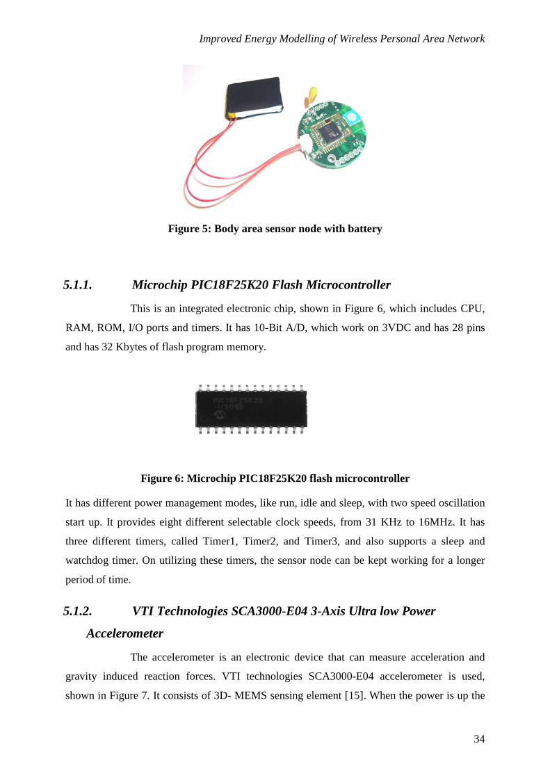
5.1.1. Microchip PIC18F25K20 Flash Microcontroller
This is an integrated electronic chip, shown in Figure 6, which includes CPU,
RAM, ROM, I/O ports and timers. It has 10-Bit A/D, which work on 3VDC and has 28 pins
and has 32 Kbytes of flash program memory.
Figure 6: Microchip PIC18F25K20 flash microcontroller
It has different power management modes, like run, idle and sleep, with two speed oscillation
start up. It provides eight different selectable clock speeds, from 31 KHz to 16MHz. It has
three different timers, called Timer1, Timer2, and Timer3, and also supports a sleep and
watchdog timer. On utilizing these timers, the sensor node can be kept working for a longer
period of time.
5.1.2. VTI Technologies SCA3000-E04 3-Axis Ultra low Power
Accelerometer
The accelerometer is an electronic device that can measure acceleration and
gravity induced reaction forces. VTI technologies SCA3000-E04 accelerometer is used,
shown in Figure 7. It consists of 3D- MEMS sensing element [15]. When the power is up the

Improved Energy Modelling of Wireless Personal Area Network
35
accelerometer starts in normal measurement mode. The accelerometer uses SPI or I2C bus for
sending information. When motion is detected, the accelerometer is activated by the pin,
called INT.
Figure 7: VTI Technologies SCA3000-E04 3-Axis accelerometer [15]
5.1.3. Free2move Low power Audio Bluetooth™ Module with antenna
F2M03ALA
Bluetooth is a short-range, wireless technology for exchange of data over 2.4
GHz ISM band (Industrial, Scientific and Medical) between two fixed or mobile devices. It
uses frequency hopping spread spectrum, which allows the transmission to be up to 79 distinct
channels.
F2M03ALA is an embedded Bluetooth module, shown in Figure 8, which has an integrated
amplifier and audio codec [16]. It has wireless UART v4 firmware. It can act both as master
and slave, in a point-to-point, and it has Piconet and scatternet capability, with a support of up
to 7 slaves. It transmits power up to +4dBm, with the possibility of restricting the output
power to 0dBm.
Figure 8: Audio Bluetooth™ module with antenna F2M03ALA. [16]
Improved Energy Modelling of Wireless Personal Area Network
36
When the device is in connecting mode, the UART firmware will try to connect to the remote
device continuously, while in endpoint mode the device may accept incoming connection
request while specified rules for establishing connection are fulfilled. It can receive a
maximum through-put of 240 Kbs, 235 Kbs and 217 Kbs, while transmitting as master to
slave, as slave to master, and as full duplex respectively.
5.1.4. Maxim DS2756 High-Accuracy Battery Fuel Gauge
DS2756 battery fuel gauge has a very small footprint that provides a certain
level of accuracy to measure the voltage, current, average current and temperature. It provides
a programmable suspend mode. Through a 1-wire interface host system, it can read/write to
status and control registers [17]. Each device has a factory-programmed 64-bit address that
allows it to be addressed individually and it supports multi battery operation [17]. In current
measurement mode, the DS2756 takes the average current of 128 individual samples after
every 88ms. In average current mode, the DS2756 takes the average of 4096 individual
current samples after every 2.8 seconds. In voltage mode, the DS2756 measures voltage
between Vin and Vss pins, over 0 to 4.75 volt range. In temperature mode, the DS2756
continuously measures the temperature and the temperature registers are updated every
220ms.
5.1.5. Battery
For back-up power to support Body area sensor node, a nominal voltage of 3.7
volts, 330mAh Lithium-Ion Polymer battery is used. It is a small and lightweight battery to
support maximum backup time.
5.2. Software
5.2.1. MPLAB IDE
MPLAB IDE is a product of Microchip for the development of embedded
applications. It is provided for free from the MPLAB website. The IDE is an integrated tool
set for the development of application for Microchip PIC and dsPIC microcontroller. It is a 32
bit application for MS Windows, and also provides the environment for third party hardware
and software development tools. MPLAB provides the same interface for all tools. It provides
the breakpoint, track and editing function. It is also color context sensitive, and just moving
the mouse on the variable or register enables the user to see the content which is saved on it.

Improved Energy Modelling of Wireless Personal Area Network
37
MPLAB IDE provides software debugging, watch window, mixed source code of Assembly
and C. It provides step in, step out and step over functions for better debugging. It has a
simulator called ‘stimulus’. The compiler, which is used to build the C or Assembly code, is
called BoostC, and it can easily integrate with MPLAB IDE.
5.2.2. MPLAB ICD 2
MPLAB ICD 2 is all in one solution; it provides a programming and debugging
environment at low cost. It provides solutions for PIC MCUs and dsPIC DSCs. Circuit
debugging is a proprietary of MPLAB. Breakpoints and watch variables can be used for
symbolic labels in Assembly and C source code. ICD 2 connects with the host PC via USB or
RS-232 Interface. It has built-in over voltage and short circuit monitor.
5.2.3. BoostC Compiler
BoostC is a C compiler that works with PIC 12, PIC 16, PIC 18. It is a
compatible compiler with ANSI C, and designed to compete with the HI-Tech C compiler. It
can be either used with SourceBoost IDE, or to integrate with MPLAB IDE.
5.3. Implementation
In the section below, the basic operations that the sensor node can perform under
normal circumstances are described.
5.3.1. Experimental Setup
In order to perform different experiments, the experimental environment is
setup with the following hardware and software.
Three additional tools are used in order to conduct experiments. These are,
� Body area sensor node (Sensor Node)
� Personal Computer
� Bluetooth™ Serial Port Plug - F2M01C1
� Docklight RS232 Terminal / RS232 Monitor Software - Version 1.8
� Agilent Digit Multimeter
The setup is briefly mentioned below.

Improved Energy Modelling of Wireless Personal Area Network
38
The personal computer, along with Bluetooth™ Serial Port Plug - F2M01C1, is used, shown
in Figure 9, which will function as base station (master), to which the sensor node will send
sensed data. One of the functions of the base station is to initiate connection with the sensor
node which is, in this case, is a Bluetooth slave (sensor node). The base station is not aware
when connection to the slave will be available, so it is always trying to get connected to the
slave when not connected.
Docklight RS232 terminal / RS232 monitor software- version 1.8 is used, which is RS232
terminal monitor software, in order to observe the received data at the base station.
Figure 9: Bluetooth™ Serial Port Plug - F2M01C1
Figure 10 shows the general flow chart of the sequence of operations on the sensor node and
Bluetooth module on the personal computer.

Improved Energy Modelling of Wireless Personal Area Network
39
Figure 10: Flow chart.

Improved Energy Modelling of Wireless Personal Area Network
40
In the next section the scenarios upon which the final system model will be based is
described.
5.4. Node Level Current Consumption
This section describes the methods used to measure the current consumption of the
sensor node with components at different states. All these individual components have already
been described in the hardware section.
The approaches followed to measure the current consumption were:
� Measurement through Agilent 34410 A 6 ½ Digit Multimeter
� Measurement through DS2756 High-Accuracy Battery Fuel Gauge
5.4.1. Measurement through Agilent 34410 A 6 ½ Digit Multimeter
The Agilent 34410 is a digital multi meter with following characteristics.
� Temperature, voltage and current measurements.
� Accuracy of 0.0030% on DC current and voltage.
� Manual and auto ranging.
� With math features like dB, null, dBm, statistics and limits.
� Data logging capability into non-volatile memory.
� Three standard remote interfaces i.e. USB, LAN and GPIB .
� Web browser bases access to instrument.
Below is the list of components, along with the different power consumption states and
current consumption, of the sensor node at these states. These measurements were taken ten
times to have the most accurate results.
Current measurements while PIC18F25K20 microcontroller in different frequencies
The current consumption of the sensor node, while the microcontroller is operating in
different frequencies, was measured. The available frequency ranges were from 31 KHz to 16
MHz. Here, the major power consumption components, like Bluetooth module and sensor
node, were turned off. The microcontroller was kept in a certain frequency for a period of
Improved Energy Modelling of Wireless Personal Area Network
41
time and the current consumption of the sensor node was measured by using digital
multimeter.
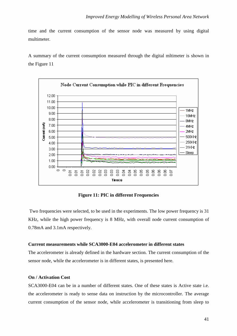
A summary of the current consumption measured through the digital mltimeter is shown in
the Figure 11
Figure 11: PIC in different Frequencies
Two frequencies were selected, to be used in the experiments. The low power frequency is 31
KHz, while the high power frequency is 8 MHz, with overall node current consumption of
0.78mA and 3.1mA respectively.
Current measurements while SCA3000-E04 accelerometer in different states
The accelerometer is already defined in the hardware section. The current consumption of the
sensor node, while the accelerometer is in different states, is presented here.
On / Activation Cost
SCA3000-E04 can be in a number of different states. One of these states is Active state i.e.
the accelerometer is ready to sense data on instruction by the microcontroller. The average
current consumption of the sensor node, while accelerometer is transitioning from sleep to
Improved Energy Modelling of Wireless Personal Area Network
42
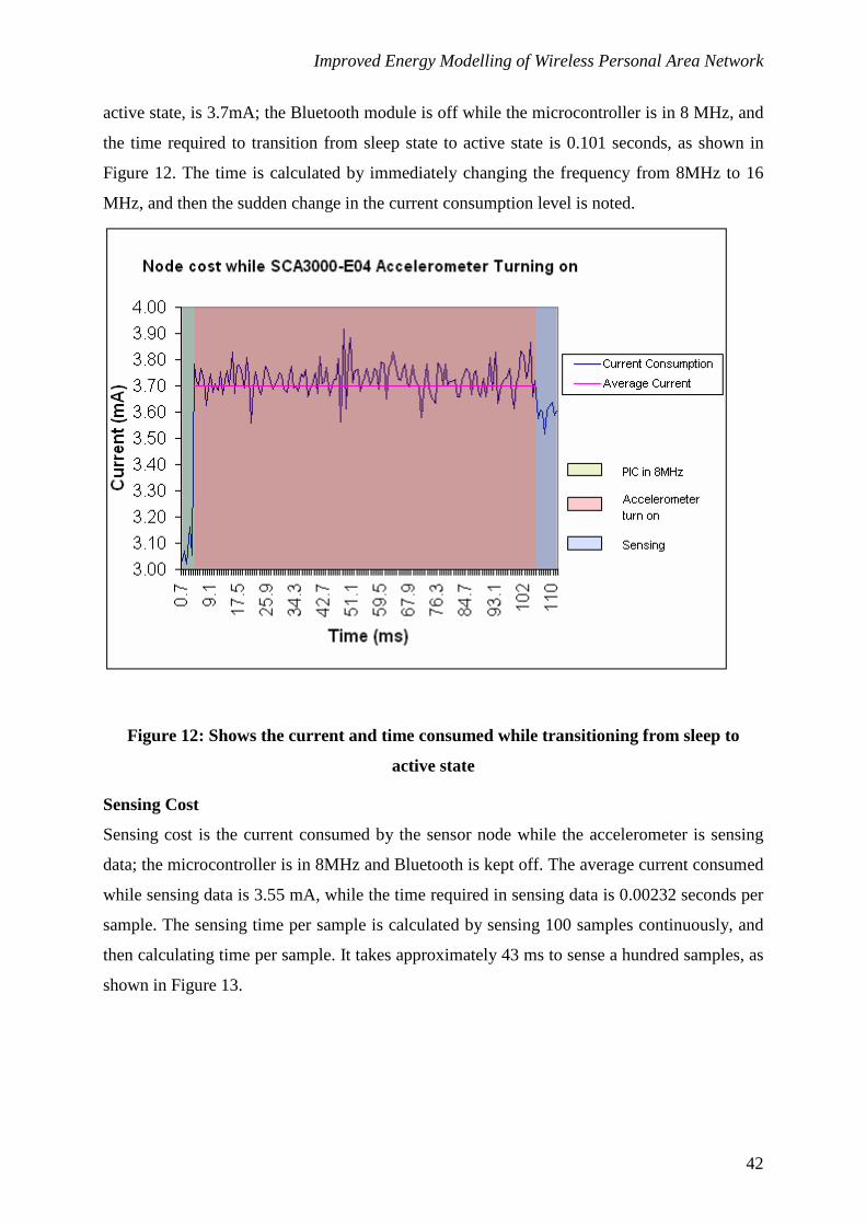
active state, is 3.7mA; the Bluetooth module is off while the microcontroller is in 8 MHz, and
the time required to transition from sleep state to active state is 0.101 seconds, as shown in
Figure 12. The time is calculated by immediately changing the frequency from 8MHz to 16
MHz, and then the sudden change in the current consumption level is noted.
Figure 12: Shows the current and time consumed while transitioning from sleep to
active state
Sensing Cost
Sensing cost is the current consumed by the sensor node while the accelerometer is sensing
data; the microcontroller is in 8MHz and Bluetooth is kept off. The average current consumed
while sensing data is 3.55 mA, while the time required in sensing data is 0.00232 seconds per
sample. The sensing time per sample is calculated by sensing 100 samples continuously, and
then calculating time per sample. It takes approximately 43 ms to sense a hundred samples, as
shown in Figure 13.

Improved Energy Modelling of Wireless Personal Area Network
43
Figure 13: Current consumed and time spends while sensing hundred samples.
Sleep Cost
Sleep state is the one with minimum current consumption. In order to transition from active
state to sleep state, the average current is approximately 2.99mA, while it takes 0.101 seconds
to transition.
Free2move F2M03ALA Bluetooth Module
The Bluetooth module can be in a number of states with different amounts of current
consumption depending upon the requirements.
Before graphically representing the current consumption at different states, certain terms will
be introduced first.
Bluetooth Turn on Cost
Bluetooth turn on cost is the cost that includes the current consumed while initializing its
circuitry, to be discovered and paired along with the time it takes to be in this state. Here, the
microcontroller is in 8MHz and the accelerometer is in sleep state. According to
measurements, the average current in turning on the Bluetooth module, while the

Improved Energy Modelling of Wireless Personal Area Network
44
microcontroller is in 8 MHz and the sensor is in sleep state, is 14.77mA, while the time
F2M03ALA used is 1.3643 seconds. The snap shot of current consumption of Bluetooth turn
on cost and time is shown in Figure 14. These measurements were done by turning on the
Bluetooth module, which is achieved by resetting the RESET pin on the Bluetooth module.
Node current consumption while Bluetooth is turned on
0
10
20
30
40
50
60
0
0.08
0.16
0.24
0.32
0.41
0.49
0.57
0.65
0.73
0.81
0.89
0.97
1.05
1.13
1.22 1.
3Time (s)
Cu
rren
t (m
A)
Figure 14: Current consumption of the sensor node while Bluetooth module is turned
on.
Connection Disconnection Cost
The connection and disconnection cost includes the current consumed while performing these
actions, along with the time spent in making this. According to measurements, the average
current consumed by the sensor node, while connecting and disconnecting a Bluetooth
connection (the accelerometer is in sleep), is 21.95mA, while the time spent is 1.0822 seconds
as shown in Figure 15.
These measurements were done by resetting the Bluetooth module, and then waiting for
connection to be established. In order to observe the connection and disconnection, two
Bluetooth ports were used. First, programmable input output pin three is used, which indicates
successful connection with the remote device. When this port is set, it indicates that the
Bluetooth connection with the remote device is established, and vice versa. When it is

Improved Energy Modelling of Wireless Personal Area Network
45
observed that the connection is established, the next step is to disconnect it, and this is
achieved by setting programmable input output pin number two, which requests the current
connection to be closed.
Node current consumption while Bluetooth is Connected & Disconnected
0
10
20
30
40
50
60
70
0
0.08
0.17
0.25
0.33
0.42 0.5
0.58
0.66
0.75
0.83
0.91 1
Time (s)
Cu
rren
t (m
A)
ConnectionDisconnection Cost
Average Current
Figure 15: Current consumed and time taken by the sensor node in connecting and
disconnecting the Bluetooth module to the base station.
Bluetooth Keep ON Cost
The sensor node has a Bluetooth module that acts as a slave, so there is a probability that the
moment the Bluetooth module at sensor node is turned on, it may not immediately get
connected to the base station (Bluetooth Master) so, in this case, it has a different current
consumption.
Figure 16 shows that the average current consumption, according to the measurement, is
5.2mA, the microcontroller is in 8 MHz and accelerometer is in sleep, while the Bluetooth is
ready to make connection with the master, and also makes a spike after every 0.82 seconds, in
case any device wants to make connection with it. The programmable input output pin
number 3 is set to low, so that it does not make a connection with any device, and the current
consumption of the sensor node is observed while the Bluetooth module is waiting for
connection.

Improved Energy Modelling of Wireless Personal Area Network
46
Bluetooth kept on
0
5
10
15
20
25
30
35
40
45
500
0.14
0.28
0.42
0.56 0.7
0.84
0.98
1.12
1.26 1.4
1.54
1.68
1.82
1.96 2.1
2.23
2.37
2.51
Time (s)
Cu
rren
t (m
A)
Figure 16: Current consumed by the sensor node while Bluetooth module is kept on
The time was calculated using graphs obtained from the Agilent digit multimeter. Transition
timing from 31 KHz to 8 MHz was calculated by changing the microcontroller frequency
from 31 KHz to 8 MHz, and plotting the graph and then, since each point on the graph was
equivalent to approximately 700 microseconds, it was easy to approximate the transition time,
and the same for 8 MHz to 31 KHz. Sensor turn on time was calculated using the same
technique. Sensor sampling time was calculated by sensing 100 samples, and then taking the
average for a single sample. A similar approach was followed for Bluetooth sending time.
Bluetooth turn on time and connection disconnection time has already been explained in the
previous section. Table 2 lists a summary of the average current measured while the
components are at different states.

Improved Energy Modelling of Wireless Personal Area Network
47
Component states Time spend Average current measurement
through Agilent multimeter
Current @ 31 KHz 7sec 0.78 mA
Current @ 8 MHz 7sec 3.1 mA
Sensor turn on 101ms 3.75 mA
Sensor sensing 0.43ms 3.55 mA
Bluetooth turn on 1.3sec 14.77 mA
Bluetooth kept on 4.2sec 4.60 mA
Bluetooth communication 0.02sec 22.55 mA
Bluetooth connection and disconnection 1.08sec 21.95 mA
Table 2: Time taken to switch from one state to another and average current measured
to perform certain functions.
5.4.2. Measurement through DS2756 fuel gauge
In order to calculate the current consumption of the individual component on
board, Dallas Semiconductor Maxim DS2756 high-accuracy battery fuel gauge is used,
providing high level of accuracy the voltage, current, average current and temperature .15 bit
average update every 2.8 seconds.
Current measurement
In order to measure the average current through the DS2756 fuel gauge, the component
should be in the particular state for 2.8 seconds, because the average current register is
updated every 2.8 seconds. For example, in order to measure the sensor node current when the
microcontroller is in 8MHz, a timer is used to keep the sensor node in this state for more than
three seconds, and then the data from the average current register is accessed. This data, i.e.
average current, is sent through Bluetooth to the base station.
Limitation
There are some limitations when measuring the average current consumption; if it is not
possible to keep the component in one state for more than 2.8 seconds, the current can not be
measured. Similarly, if the switching between different states takes less than 2.8 seconds, this
current can not be measured. For example, the Bluetooth module takes 1.36 to turn ON but
the average current register takes 2.8 seconds to be updated. It is possible to take the average

Improved Energy Modelling of Wireless Personal Area Network
48
current, but it may not be accurate since the average current may contain current, while the
sensor node is in some other state. That is why table 4 has some with ‘not applicable (NA)’
entries.
Time Measurement
In order to validate the model, the time spent in each component state shall also be known, for
example, how much time the component will take to turn ON and turn OFF. Time
measurement is also done in two ways.
� Using Agilent multimeter
� Using internal timer
Agilent multimeter has the ability to sample data every 700 micro seconds and, by using this
data, it is easily possible to know how much time any component takes to do any kind of
activity.
In order to calculate how much time the component takes to turn itself ON or OFF,
microcontroller frequency is used. At 8MHz, the MCU takes 0.5 microseconds for one cycle.
According to this, it takes 1ms/0.5 microseconds = 2000 cycles in one milliseconds. At 31
KHz, the MCU takes 0.125ms in one cycle and 1ms/0.125 milliseconds = 8 cycle in one
milliseconds.
The timer function can be used to calculate how much time the component takes to turn ON
or OFF. Before turning ON or OFF a component the timer is set to zero and the number of
cycles are measured when the component is turned ON. Table 3 shows the comparison
between the current measured through the DS2756 fuel gauge, and the digit multimeter.

Improved Energy Modelling of Wireless Personal Area Network
49
Component states Timer Time DS fuel
gauge
Agilent digit multimeter
readings
Current @ 31 KHz 7sec 7sec 0.78 mA 0.78 mA
Current @ 8 MHz 7sec 7sec 3.3 mA 3.1 mA
Sensor turn on 101ms 101ms 3.7 mA 3.75 mA
Sensor sensing 43ms 43ms 3.6 mA 3.55 mA
Bluetooth turn on NA 1.36sec NA 14.77 mA
Bluetooth keep on NA 1.80sec NA 4.60 mA
Bluetooth communication 0.03sec 0.02sec 22.3 mA 22.55 mA
Bluetooth connection and
disconnection NA 1.08sec NA 21.95 mA
Table 3: Comparison of the individual current consumption using DS2756 Fuel Gauge
and Agilent Digit Multimeter.
Through comparison of the current consumptions through a digit multimeter and a DS2756
fuel gauge, the accuracy of the DS2756 fuel gauge is verified. It proves its importance and
restriction in future design of the systems based upon the proposed model. In most of the
cases, the deviation between the current readings through a digit multimeter and DS2756 are
found to be very close.
5.5. Model level Current Consumption
Now the current and time for each individual component is calculated it can be
considered. The next section will describe the life time prediction of the sensor node through
the proposed model.
Here, two approaches are followed. One is calculating the life time of the sensor node at
different states, by actually depleting the physical battery. The other is by calculation of life
time through the current consumption of the individual components.
Scenarios
This section describes different scenarios which were included in the experiments.
All these scenarios were tested with a fully charged battery i.e. 4.1 Volts.

Improved Energy Modelling of Wireless Personal Area Network
50
� Low Power Mode - Sensing
� Sensing
� Communication
� Low Power Mode – Communication
5.5.1. Low Power Mode – Sensing
Low Power mode, as mentioned earlier in section 4, is a state where the PIC
microcontroller is in 31 KHz frequency, and both the Bluetooth and sensor modules are off.
This is the state with the minimum current consumption.
The sensing state is the one where the sensor is sensing and also the microcontroller is in 8
MHz. The sensor node stays in the low power mode for 100 milliseconds, and then turns on
the sensor module, which takes approximately 101 ms, senses data and turns off the sensor
module, and then transitions back to low power mode. Figure 17 shows the current and time
spent when the sensor node transitions from Low power mode to Sensing mode.
Low Power Mode - Sensing Mode
0
0.5
1
1.5
2
2.5
3
3.5
4
4.5
0.7 21
41.3
61.6
81.9
102
123
143
163
183
204
224
244
265
285
305
326
346
time (ms)
Cu
rren
t (m
A)
LPM
Accelerometer turn on Sensing Pow er
Accelerometer turn off
T0
T1T2
T3
T0 Time in LPM
T3 Time spent in turing off accelerometer
T2 Time spent w hile sensing
T1 Time w hile turning on accelerometer
Figure 17: Current consumption by sensor node while in Low power mode to Sensing mode.

Improved Energy Modelling of Wireless Personal Area Network
51
5.5.2. Sensing
As mentioned earlier, the sensing state is the one where the PIC is in 8 MHz
and the sensor is active and can sense data. Here, the sensor is kept active, as it is the
requirement of the system to be in this state, and then it senses every 300 milliseconds.
5.5.3. Communication
The Communication mode is the one that has the microcontroller in high
frequency, i.e. 8 MHz, while the sensor is OFF and Bluetooth is ON and connected to
transmit data. So, in this scenario, the Bluetooth is kept active and sends data every three
seconds.
5.5.4. Low Power Mode – Communication
The low power mode and communication mode are already described. In this
scenario, the system is in low power mode for 1.1662 seconds, then the frequency is changed
from 31 KHz to 8 MHz, the Bluetooth module is turned on, which takes around 1.36 seconds,
then it tries to get connected to the Bluetooth module at the base station, and then it sends the
already sensed data by the sensor. This cycle continues, i.e. it transitions back to low power
mode and so on, as shown in Figure 18.

Improved Energy Modelling of Wireless Personal Area Network
52
Low Power Mode - Communication
0
10
20
30
40
50
60
700
0.66
1.32
1.98
2.65
3.31
3.97
4.63
5.29
5.95
6.61
7.27
7.94 8.6
9.26
9.92
10.6
11.2
11.9
Time (s)
Cu
rren
t (m
A)
Figure 18: Current consumption while the sensor node is in LMP, Communication and
while transitioning from LPM to Communication.
Table 4 lists down the results obtained by actually depleting the battery when the sensor node
is at different states.
Scenario Description Results
(Actual Life Time)
1 Low Power Mode Sensing Mode 161 hr
2 Sensing Mode 75 hr
3 Low Power Mode Communication Mode 24 hr
4 Communication Mode 17 hr
Table 4: Summary life time with different Scenarios
Now that the actual current consumption of the sensor node with components at different
states is measured (Table 2), the next step would be to try to differentiate between the life
time predictions when the actual current consumption, while transitioning, is catered for, and
when it is not catered for.

Improved Energy Modelling of Wireless Personal Area Network
53
Sensor node life time is estimated with and without utilizing the switching cost. The average
current consumption per cycle is calculated by ratio of each component time to total cycle
time in particular state times, the average current consumed in the particular state during that
particular cycle e.g. in case of low power mode – Sensing scenario the current consumed by
the sensor node when the microcontroller is in 31 KHz i.e. Low power mode, while
accelerometer and Bluetooth modules are off is 0.78mA and the current consumed by the
sensor node when the sensor is active and sensing data i.e. Sensing mode, while the
microcontroller is in 8MHz and Bluetooth is off is 3.55mA.
The life time prediction, where switching cost is catered for, the average current during the
switching is measured and multiplied with the ratio of switching time to total cycle time, i.e.
in this case, current consumption are 3.7mA and 3.55mA, while turning on and off the
accelerometer.
There are three different approaches to compensate/ predict the switching cost in cases where
the actual current consumption during switching is not catered for. These are:
� Best case
� Average
� Worst case
In the best case, the switching time which is 0.202 seconds (it is the time taken to turn on the
accelerometer and to turn off the accelerometer), in case of low power mode – sensing mode,
is added to the time in Low power mode and the calculations are performed, as explained in
preceding paragraph. It is called the ‘best case’ because the time is added to the mode with
least power consumption.
In an average case, this time is equally divided and half the time is added to time in Sensing
mode, and half in low power mode.
In the worst case, this time is added to the time in sensing mode. It is called ‘worst case’ since
the time is added to the mode which is the more power consuming. A similar approach was
followed for the low power mode – communication.

Improved Energy Modelling of Wireless Personal Area Network
54
In this way, the contribution of each and every component in one single cycle is calculated.
The next step is to add all this individual contribution, and divide the total battery capacity by
the average. Here, the life time prediction of each of these scenarios is mentioned in Table 5,
and, for a detailed description, refer to appendix A.
Results with out Transitions*
Scenario Description
Results
(Actual
Life
Time)
Best Case
Average Case
Worst Case
Results with Transition*
1 Low Power Mode
Sensing Mode 161 hr 412 hr 197 hr 130 hr 136 hr
2 Sensing Mode 75 hr 75 hr 75 hr 75 hr 75 hr
3
Low Power Mode
Communication
Mode
24 hr 362 hr 38 hr 20 hr 28 hr
4 Communication
Mode 17 hr 17 hr 17 hr 17 hr 17 hr
* The calculations are given in appendix A.
Table 5: Compares the life time prediction at different scenarios and using different
calculation approaches.

Improved Energy Modelling of Wireless Personal Area Network
55
6. Summary
The aim of this thesis was to depict the importance of transition cost, which included both
time and energy consumption, from one logical state to another. In order to achieve this goal,
the sensor node is analyzed component-wise, then the logical states were defined and the
current consumption of these individual states estimated. The next step was to further improve
and formulate the current consumption of the sensor node with individual components in
different states, so that the life time of the battery, when run in different scenarios, could be
predicted. All of these scenarios were verified with actual physical settings.
6.1. Better Life Time Prediction
An important result from the research work was the accurate prediction of a battery’s
life time. If only the current consumption of individual states is considered, rather than both
the current consumption in the states and the transition, the life time prediction can not be
accurately predicted if however, this feature is considered, the life time prediction can be
improved up to an average of 85 %. The results are extremely encouraging in case of scenario
one, where better life time prediction is achieved in contrast to worst case life time prediction.
On the other hand on comparison with best case the life time prediction is improved from 412
hours to 136 hours, while the actual calculated life time was 161 hours approximately. The
life time prediction for scenario 3 in comparison to worst case was the same. Table 5
compares the life time prediction at different scenarios and using different calculation
approach.
6.2. Better Threshold Prediction
Another important result from the research work was the ability to define the
threshold in terms of time. A threshold can be better understood in terms of accelerometer
switching time, as it is known that the accelerometer takes 0.202 seconds to switch so, if an
application has a requirement of sensing ever 0.100 seconds, then it is not possible to switch
the accelerometer. Rather, it can be said that the threshold is at least 0.202 seconds.
Table 2 shows that the time to reset the Bluetooth, and trying to get connected to the
Bluetooth base station, is approximately 3 seconds, which includes Bluetooth turn on time,
Bluetooth wait for connection time, Bluetooth connection and disconnection time. So the
decision to turn off is firstly greatly influenced by reset time, the waiting for connection time

Improved Energy Modelling of Wireless Personal Area Network
56
and connection disconnection time. If it is decided to turn off the Bluetooth in order to save
power, it must be assured that the transmission time is greater than the reset time, connection
disconnection and the waiting for connection time. Any transmission time of less than 3
seconds will allow the system to be in communication state, which is to be connected to the
master or base station, and this state is the one with highest power consumption.
Like the accelerometer, the Bluetooth module also imposes a bottom line for sensing rate. If
Bluetooth switching time is increased, the advantages and disadvantage of having shorter and
longer switching times are known. Figure 19 shows that the switching time is inversely
proportional to the life time i.e. greater the switching time shorter the life time. As the
switching time reaches 4 seconds, any increase in switching time almost has an almost
negligible impact on the life time.
An important result after analyzing is that, in order to improve the life time of the battery, the
switching time must be reduced, otherwise this will remain as a bottle neck.
Figure 19: Life time prediction

Improved Energy Modelling of Wireless Personal Area Network
57
7. Discussion
In this section, a discussion about the usage of the proposed model is presented. The thesis
investigates the importance of switching cost, because this aspect was not covered in the
previous work. Different questions could arise in the mind, like what effect can it have if the
switching cost is not considered at all? And how much effect does the switching cost have If
the switching of a sensor’s component from one state to another is not feasible, then it is
worth keeping it in that state.
The end result was that switching cost is an important factor to consider. Especially while
predicting the life time of the sensor node, and while the switching cost is investigated in
terms of time and current consumption, the limitation in performance was known if the
components in a sensor node have to switch.
Reducing the switching time can increase the life time of the sensor node. It can be used as a
tool for programmers who know application-specific information, like the sampling rate, and
the transmission rate. Since this can benefit them in deciding when to switch the component,
and how long to stay in one state e.g. in case of low power mode to sensing mode, if the
application requirement is to sense every 100 milliseconds, the application can dictate to stay
in sensing mode, and vice versa.
Secondly it can be used to predict the life time of the sensor node if the switching time is
decreased in the future. It gives an accurate prediction of the life time even before actually
implementing it in the environment.
The extension of this proposed model can be, for hardware components where the time and
current consumption while switching varies, is to have dynamic current measurements
through DS2756 fuel gauge. In this way more accurate results can be obtained.

Improved Energy Modelling of Wireless Personal Area Network
58

Improved Energy Modelling of Wireless Personal Area Network
59
8. Conclusion
This thesis started aimed to verify the hypothesis that current consumption while
switching from one sensor state to another influence the life time. This aspect was previously
being ignored in other research work. A model was proposed which had a number of modes,
and each mode was defined with components in different states. These states were low power
mode, sensing, communication and full power mode. In order to prove this, the hardware
must have the property of being able to switch between different states, and the switching
between these sates shall be costly.
The proposed model was build. Analysis started from the individual component level. Tools
like the digital multimeter were used to perform different experiments. The life time
prediction through these experiments was compared. The life time prediction of the sensor
node with a given battery was quite accurate.
Switching cost is an important factor is determining the life time of the sensor node. The life
time of the sensor node can further be improved if the switching time is improved. In case of
Bluetooth, if the requirement is to transmit data less then 3 seconds, then the life time will be
restricted, and if the requirement is to transmit after 3 seconds, then the life time can be
improved significantly. From this study we can say that only by a delay of 1 second
significantly increases the life time.
Not only the focus shall be on the switching time, but also the current consumed while
switching. Figure 19 shows the life time prediction, while the current consumption of
switching is the same but the switching time varies. So the life time can be further improved
by improving the current consumed while switching.
DS2756 fuel gauge can be used, with some limitation, to estimate the life time of the sensor
node.

Improved Energy Modelling of Wireless Personal Area Network
60

Improved Energy Modelling of Wireless Personal Area Network
61
9. References
[1] Roomer, Kay; Friedman Mattern. "The Design Space of Wireless Sensor Networks".
IEEE Wireless Communications 11 (6) Dec. 2004 54-61
[2] Thomas Haenselmann (2006-04-05). "Sensor networks". GFDL Wireless Sensor
Network textbook. Retrieved on 2006-08-29.
[3] Sinha, A. Chandrakasan, A. Dynamic power management in wireless sensor networks.
IEEE Design and Test of Computers, vol. 18, Issue 2, pp. 62-74, March-April, 2001
[4] S. Hadim and N. Mohamed. Middleware Middleware challenges and approaches for
wireless sensor networks. IEEE Distributed Systems Online, 7(3), 2006. art. no. 0603-
o3001.
[5] K. Romer, .Programming paradigms and middleware for sensor networks,. in GI/ITG
Workshop on sensor networks, Karlsruhe, Germany, pp. pp. 49.54, February, 2004.
[6] Ana Luiza de A.P. Efficient Power Management in Real-Time Embedded Systems
[7] W Wolf Computer as Components – Principles of embedded computing systems
Design. Morgan Kaufman Publishers.
[8] Hempstead M, Tripathi N, Mauro P, Wei G, and Brooks D, "An Ultra Low Power
System Architecture for Wireless Sensor Network Applications," 32nd International
Symposium on Computer Architecture (ISCA-05), June 2005.
[9] T. Massey, F Dabiri, R Jafari, H Noshadi, P Brisk, W Kaiser, M Sarrafzadeh,
Towards Reconfigurable Embedded Medical Systems High Confidence Medical
Devices, Software, and Systems and Medical Device Plug-and-Play Interoperability,
2007. HCMDSS-MDPnP. Joint Workshop on volume, Issue , 25-27 June 2007
Page(s) 178 – 180
[10] B. Bougard, F. Catthoor, D. C. Daly, A. Chandrakasan, and W. Dehaene, “Energy
efficiency of the IEEE 802.15.4 standard in dense wireless microsensor networks
Modeling and improvement perspectives,” in Proc of Design, Automation, and Test in
Europe (DATE), 2005.
[11] R.M. Passos, C.J.N. Coelho, A.A.F. Loureiro, R.A.F. Mini, "Dynamic Power
Management in wireless Sensor Networks An Application-Driven Approach," In
Proc. of the 2nd Annu. conference on Wireless On-demand Network Systems and
Services (WONS '05), pp. 109 - 118, 19-21 Jan. 2005.
[12] Margi, C. B., Petkov, V., Obraczka, K., and Manduchi, R. (2006). Characterizing
energy consumption in a visual sensor network testbed. In 2nd International

Improved Energy Modelling of Wireless Personal Area Network
62
IEEE/Create-Ne Conference on Testbeds and Research Infrastructures for the
Development of Networks and Communities (TridentCom 2006), Barcelona, Spain.
[13] X. Yu, K. Niyogi, S. Mehrotra, and N. Venkatasubramanian, .Adaptive middleware
for distributed sensor environments,. IEEE DS Online, 2003.
[14] V. Shnayder et al. Simulating the Power Consumption of Large-Scale Sensor Network
Applications. In Proc. of Sen-Sys, Nov. 2004.
[15] VTI Technologies SCA3000 Series 3-axis accelerometer Doc.Nr. 8257300A.06 Data
Sheet.
[16] Free2move Low power Audio Bluetooth™ Module with antenna F2M03ALA
Preliminary datasheet Rev 0 Data sheet.
[17] Dallas Semiconductor Maxim DS2756 High-Accuracy Battery Fuel Gauge
With Programmable Suspend Mode PDF

Improved Energy Modelling of Wireless Personal Area Network
63
Appendix A
Low Power Mode- Sensing Mode (With out Transition Cost)
Sensor node Current consumption while in 31KHz C31 = 0.78mA
Sensor node Current consumption while in 8MHz C8 = 3.1mA
Sensor node Current consumption while sensing Cs = 0.45mA
Time spend in 31 KHz (LPM) TL = 0.11 sec
Time spent while sensing one sample Ts = 0.002 sec
Time spent in switching Tsw = 0.20 sec
Worst case Time Tw = Ts + Tsw
Best case Time Tb = TL + Tsw
Average case Time Ta = Tsw /2
Total energy = 330mAh
Total time T = 0.32 seconds
Worst case Current Consumption/Cycle = C31 TL / T + (C8+Cs) Tw / T
= 2.54
Best case Current Consumption/Cycle = C31 Tb / T + (C8+Cs) Ts / T
= 0.80
Average case Current Consumption/Cycle = C31 (TL+ Ta) / T + (C8+Cs) (Ts + Ta) / T
= 1.67
Life time with Worst case = Total energy / Current per cycle = 130hr
Life time with Best case = Total energy / Current per cycle = 412hr
Life time with Average case = Total energy / Current per cycle = 197hr

Improved Energy Modelling of Wireless Personal Area Network
64
Low Power (Sensing with Transition cost)
Sensor node Current consumption while in 31KHz C31 = 0.78mA
Sensor node Current consumption while in 8MHz C8 = 3.1mA
Sensor node Current consumption while sensing CS = 0.45mA
Sensor node current consumption while turning ON accelerometer CSON = 3.7mA
Sensor node current consumption while turning OFF accelerometer CSOFF = 2.99mA
Time spend in 31KHz (LPM) TL = 0.11 sec
Time spend while sensing one sample TS = 0.002 sec
Sensor time spent while turning ON TSON = 0.10sec
Sensor time spent while turning OFF TSOFF = 0.10sec
Total energy = 330 mAh
Total time T = 0.32 seconds
Current Consumption/ Cycle = C31 TL/ T +(C8+CS) TS / T + CSON TSON / T + CSOFF TSOFF / T
= 2.41
Life time = Total energy / Current per cycle = 136hr

Improved Energy Modelling of Wireless Personal Area Network
65
Low Power – Communication (With out Transition)
Current consumption while 8MHz C8 = 3.1mA
Current consumption while 31KHz C31 = 0.78mA
Current consumption while sending CBS = 22.5588mA
Time spend while sending TSB = 0.02476 sec
Time spend in low power mode TL = 1.1662 sec
Time spent in switching Tsw = 2.93 sec
Worst case Time Tw = TSB + Tsw
Best case Time Tb = TL + Tsw
Average case Time Ta = Tsw /2
Total time T = 4.12886 sec
Total energy = 330mAh
Worst case Current Consumption/Cycle = C31TL / T + CBS Tw / T
= 16.40
Best case Current Consumption/Cycle = C31 Tb / T + CBS TSB / T
= 0.91
Average case Current Consumption/Cycle = C31TL (TL +Ta)/ T + CBS (TSB +Ta )/ T
= 8.66
Life time with Worst case = Total energy / Current per cycle = 20hr
Life time with Best case = Total energy / Current per cycle = 362hr
Life time with Average case = Total energy / Current per cycle = 38hr
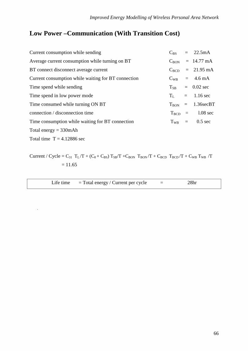
Improved Energy Modelling of Wireless Personal Area Network
66
Low Power –Communication (With Transition Cost)
Current consumption while sending CBS = 22.5mA
Average current consumption while turning on BT CBON = 14.77 mA
BT connect disconnect average current CBCD = 21.95 mA
Current consumption while waiting for BT connection CWB = 4.6 mA
Time spend while sending TSB = 0.02 sec
Time spend in low power mode TL = 1.16 sec
Time consumed while turning ON BT TBON = 1.36secBT
connection / disconnection time TBCD = l.08 sec
Time consumption while waiting for BT connection TWB = 0.5 sec
Total energy = 330mAh
Total time T = 4.12886 sec
Current / Cycle = C31 TL /T + (C8 + CBS) TSB/T +CBON TBON /T + CBCD TBCD /T + CWB TWB /T
= 11.65
Life time = Total energy / Current per cycle = 28hr
.