improved digital watermarking schemes … digital watermarking schemes using dct and neural...
TRANSCRIPT

IMPROVED DIGITAL WATERMARKING SCHEMES
USING DCT AND NEURAL TECHNIQUES
A THESIS SUBMITTED IN PARTIAL FULFILLMENT
OF THE REQUIREMENTS FOR THE DEGREE OF
Bachelor of Technology
In
Computer Science and Engineering
By
Hitesh Agarwal
Roll No: 10206006
Sapan Kumar Panda
Roll No: 10306019
Jayachandra Behera
Roll No: 10306021
Department of Computer Science and Engineering
National Institute of Technology
Rourkela
2007

i
IMPROVED DIGITAL WATERMARKING SCHEMES
USING DCT AND NEURAL TECHNIQUES
A THESIS SUBMITTED IN PARTIAL FULFILLMENT
OF THE REQUIREMENTS FOR THE DEGREE OF
Bachelor of Technology
In
Computer Science and Engineering
By
Hitesh Agarwal
Roll No: 10206006
Sapan Kumar Panda
Roll No: 10306019
Jayachandra Behera
Roll No: 10306021
Under the Guidance of
Prof. R.Baliarsingh
Department of Computer Science and Engineering
National Institute of Technology
Rourkela
2007

ii
National Institute of Technology Rourkela
CERTIFICATE
This is to certify that the thesis entitled, “IMPROVED DIGITAL WATERMARKING
SCHEMES USING DCT AND NEURAL NETWORKS” submitted by Hitesh Agarwal, Sapan
Kumar Panda and Jayachandra Behera in partial fulfillment of the requirements for the award of
Bachelor of Technology Degree in Computer Science and Engineering at the National Institute
of Technology, Rourkela (Deemed University) is an authentic work carried out by them under
my supervision and guidance.
To the best of my knowledge, the matter embodied in the thesis has not been submitted to any
other university / institute for the award of any Degree or Diploma.
Date : 10 May ,2007 Prof. R.Baliarsingh Dept. of Computer Science and Engineering
National Institute of Technology Rourkela - 769008
iii
ACKNOWLEDGEMENT
We express our sincere gratitude and indebtedness to Dr. R.Baliarsingh, Professor in the
department of Computer Science and Engineering, NIT Rourkela for giving us the opportunity to
work under him and extending every support possible at each stage of this project work. The
level of flexibility offered by him in implementing the project work is highly applaudable.
We would also like to convey our deep regards to all other faculty members and staff of
Department of Computer Science and Engineering, NIT Rourkela, who bestowed their great
effort and guidance at appropriate times without which it would have been very difficult on our
part to finish the project work.
Last but not the least we are indebted to our parents for inspiration and all of our friends
who patiently extended all sorts of help for accomplishing this undertaking.
Date: May 10, 2007 Hitesh Agarwal
Sapan Kumar Panda
Jayachandra Behera
Dept. of Computer Science Engineering
National Institute of Technology
Rourkela - 769008

iv
CONTENTS Page No
Abstract v List of Figures vii List of Tables viii
Chapter 1 General Introduction 1
1.1 Background 2
1.2 Motivation for Digital Watermarking 3
1.3 Layout of the Thesis 4
Chapter 2 Characteristics, Applications & Classification 5
2.1 Characteristics of Digital Watermarking 6
2.2 Applications of Digital Watermarking 7
2.3 Classification of Digital Watermarking technique 8
2.4 Framework and parameters of Digital Watermarking 9
Chapter 3 Digital Watermarking Techniques Classification 12
3.1 Techniques in Spatial domain 13
3.2 Techniques in Frequency domain 14
3.3 Experimental results 17
3.4 Conclusion 19
Chapter 4 Digital Watermarking using Neural Network 20
4.1 Watermarking using Back Propagation Network 21
4.2 Proposed method using RBFNN 26
4.3 Experimental Results 35
4.4 Discussion 38
4.5 Conclusion 39
Chapter 5 Conclusion 40
REFERENCES 42

v
ABSTRACT
The present thesis investigates the copyright protection by utilizing the digital watermarking of
images. The basic spatial domain technique DCT based frequency based technique were studied
and simulated. Most recently used Neural Network based DCT Scheme is also studied and
simulated. The earlier used Back Propagation Network (BPN) is replaced by Radial Basis
Function Neural Network (RBFNN) in the proposed scheme to improve the robustness and
overall computation requirements. Since RBFNN requires less number of weights during
training, the memory requirement is also less as compared to BPN.
Keywords : Digital Watermarking, Back Propagation Network (BPN), Hash Function,
Radial Basis Function Neural Network (RBFNN), and Discrete Cosine Transform (DCT).
Watermarking can be considered as a special technique of steganography where one
message is embedded in another and the two messages are related to each other in some way.
The most common examples of watermarking are the presence of specific patterns in currency
notes, which are visible only when the note is held to light, and logos in the background of
printed text documents. The watermarking techniques prevent forgery and unauthorized
replication of physical objects.
In digital watermarking a low-energy signal is imperceptibly embedded in another signal.
The low-energy signal is called the watermark and it depicts some metadata, like security or
rights information about the main signal. The main signal in which the watermark is embedded is
referred to as the cover signal since it covers the watermark. In recent years the ease with
which perfect copies can be made has lead large-scale unauthorized copying, which is a great
concern to the music, film, book and software publishing industries. Because of this concern
over copyright issues, a number of technologies are being developed to protect against illegal
copying. One of these technologies is the use of digital watermarks. Watermarking embeds an
ownership signal directly into the data. In this way, the signal is always present with the data.

vi
Analysis
Digital watermarking techniques were implemented in the frequency domain using Discrete
Cosine Transform (DCT).The DCT transforms a signal or image from the spatial domain to the
frequency domain. Also digital watermarking was implemented using Neural Networks such as:
1. Back Propagation Network (BPN)
2. Radial Basis Function Neural Network (RBFNN)
Digital watermarking using RBFNN was proposed which improves both security and robustness
of the image. It is based on the Cover’s theorem which states that nonlinearly separable patterns
can be separated linearly if the pattern is cast nonlinearly into a higher dimensional space.
RBFNN contains an input layer, a hidden layer with nonlinear activation functions and an output
layer with linear activation functions.
Results
The following results were obtained:-
1. The DCT based method is more robust than that of the LSB based method in the tested
possible attacks. DCT method can achieve the following two goals: The first is that
illegal users do not know the location of the embedded watermark in the image. The
second is that a legal user can retrieve the embedded watermark from the altered image.
2. The RBFNN network is easier to train than the BPN network. The main advantage of the
RBFNN over the BPN is the reduced computational cost in the training stage, while
maintaining a good performance of approximation. Also less number of weights are
required to be stored or less memory requirements for the verification and testing in a
later stage.

vii
LIST OF FIGURES
Figure no. Name Page
1.1 Digital Watermarking System 3
2.1 Embedding Watermark 10
2.2 Detecting Watermark 10
3.1 Defination of DCT Regions 15
3.2 DCT Based Watermark 16
3.3 Result Images of DCT Based Method 18
4.1 Architecture of a BPN network 22
4.2 Layout of a single neuron 22
4.3 BPN Model used for Watermarking 23
4.4 Result Images of BPN-DCT Based Method 25
4.5 Radial Basis Neural Network Architecture 27
4.6 Selected overlapped DCT blocks 32
4.7 Number of AC Components 32
4.8 RBFNN Model used for watermarking 33
4.9 Variations of the MSE (Mean Square Error) 35
4.10 Result Images of RBFNN-DCT Based Method 37

viii
LIST OF TABLES
Table No
Name Page
2.1 Classification of Watermarking according to several viewpoints 8
3.1 BCR % and PSNR (dB) of different test images in LSB and DCT methods 19
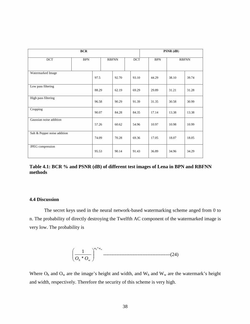
4.1 BCR % and PSNR (dB) of different test images in BPN and RBFNN methods
38

1
Chapter 1
GENERAL INTRODUCTION
1.1 Background
1.2 Motivation for Digital Watermarking
1.3 Layout of the Thesis
2
INTRODUCTION 1.1 Background
Watermarking is not a new technique. It is a descendent of a technique known as
steganography, which has been in existence for at least a few hundred years. Steganography is a
technique for concealed communication. In contrast to cryptography where the content of a
communicated message is secret, in steganography the very existence of the message is a secret
and only parties involved in the communication know its presence. Steganography is a technique
where a secret message is hidden within another unrelated message and then communicated to
the other party. Some of the techniques of steganography like use of invisible ink, word spacing
patterns in a printed document, coding messages in music compositions, etc. have been used by
military intelligence since the times of ancient Greek civilization.
Watermarking can be considered as a special technique of steganography where one
message is embedded in another and the two messages are related to each other in some way.
The most common examples of watermarking are the presence of specific patterns in currency
notes, which are visible only when the note is held to light, and logos in the background of
printed text documents. The watermarking techniques prevent forgery and unauthorized
replication of physical objects.
Digital watermarking is similar to watermarking physical objects except that the
watermarking technique is used for digital content instead of physical objects. In digital
watermarking a low-energy signal is imperceptibly embedded in another signal. The low-energy
signal is called the watermark and it depicts some metadata, like security or rights information
about the main signal. The main signal in which the watermark is embedded is referred to as the
cover signal since it covers the watermark. The cover signal is generally a still image, audio clip,
video sequence or a text document in digital format.
The digital watermarking system essentially consists of a watermark embedder and a
watermark detector (fig 1.1). The watermark embedder inserts a watermark into the cover signal
and the watermark detector detects the presence of watermark signal. Note that the entity called
the watermark key is used during the process of embedding and detecting watermarks. The
watermark key has a one-to-one correspondence with the watermark signal (i.e. a unique
watermark key exists for every watermark signal). The watermark key is private and known to

3
the authorized parties and it ensures that only the authorized parties can detect the watermark.
Further, note that the communication channel can be noisy and hostile (i.e. is prone to attacks)
and hence the digital watermarking techniques should be resilient to both noise as well as
security attacks.
Watermark key noise attacks watermark key
watermark signal watermark Fig 1.1: Digital Watermarking System
Definitions
Throughout this thesis, the notation and terminologies are used as per the definition
specified at the first International Workshop of Information Hiding.
The information to be hidden (watermark, or in the general case of steganography, a
secret message) embedded in a cover object (a cover CD, video or text), giving a stego object,
which we may also call a marked object.
The embedding is performed with the help of a key, a secret variable that is in general
known to the object’s owner. Recovery of the embedded watermark may or may not require a
key. If it does, the key may be equal to or derived from the key used in the embedding process.
1.2 Motivation for Digital Watermarking
In recent years it has been seen a rapid growth in network multimedia systems and other
numerical technologies. This has led to an increasing awareness of how easy it is becoming to
reproduce data. The ease with which perfect copies can be made may lead large-scale
unauthorized copying, which is a great concern to the music, film, book and software publishing
industries.

4
Because of this concern over copyright issues, a number of technologies are being
developed to protect against illegal copying. One of these technologies is the use of digital
watermarks. Watermarking embeds an ownership signal directly into the data. In this way, the
signal is always present with the data.
Problems with Cryptography as a solution:
Many of the problems that we need to solve in enforcing copyright law for digital content
are similar to problems in secure communications that have been solved using cryptography. For
example, we may want to guarantee the integrity of the digital content when it is distributed, so
that we can detect if it has been altered. Cryptography has also solved this problem called non-
repudiation, in secure communications. Traditional cryptosystems suffer from one important
drawback, however, which renders them useless for the purpose of enforcing copyright law: they
do not permanently associate cryptographic information with content. Cryptographic techniques
can hide a message from plain view during communication, and can also provide auxiliary
information that effectively proves the message’s integrity and guarantees non-repudiation;
however cryptography does not embed information directly into the message itself. Thus
cryptography alone can not make any guarantees about the redistribution or alteration of the
content after it has initially passed through the cryptosystem. To provide the extended guarantees
about the digital content, we need to extend the cryptographic techniques and embed additional
information in the content itself. The techniques that have been proposed for solving this
problem are collectively called digital watermarking.
1.3 Layout of the Thesis
The thesis report is organized as follows: Chapter 2 describes the Characteristics,
Applications and Classifications of Digital watermarking. Chapter 3 deals with different
watermarking techniques and also simulation results of the basic techniques like LSB
modification and DCT based watermarking. Chapter 4 discusses the existing techniques of
watermarking using MLPNN in DCT domain and the proposed RBFNN and DCT based
algorithm and the results obtained thereof. Finally chapters 5 and 6 deal with conclusion of
overall work and future enhancements.

5
Chapter 2
CHARACTERISTICS, APPLICATIONS AND
CLASSIFICATIONS OF DIGITAL WATERMARKING
2.1 Characteristics of Digital Watermarking
2.2 Applications of Digital Watermarking
2.3 Classification of Digital Watermarking technique
2.4 Framework and parameters of Digital Watermarking

6
2.1 Characteristics of Digital Watermarking
Digital watermarking techniques have the following main features for embedding
metadata in multimedia content
• Imperceptibility: The embedded watermarks are imperceptible both perceptually as well
as statistically and do not alter the aesthetics of the multimedia content that is watermarked. The
watermarks do not create visible artifacts in still images, alter the bit rate of the video or
introduce audible frequencies in audio signals.
• Robustness: Depending on the application, the digital watermarking technique can
support different levels of robustness against changes made to the watermarked image. If digital
watermarking is used for ownership identification, then the watermark has to be robust against
any modifications. The watermarks should not get degraded or destroyed as a result of
unintentional or malicious signal and geometric distortions like analog-to digital conversions,
digital-to-analog conversion, cropping, resampling, rotation, scaling and compression of the
content. On the other hand, if it is used for content authentication, the watermarks should be
fragile i.e. it should get destroyed whenever the content is modified so that any modification to
content can be detected.
• Inseparability: After the digital content is embedded with watermark, separating the
content from the watermark to retrieve the original content is not possible.
• Security: The digital watermarking techniques prevent unauthorized users from detecting
and modifying the watermark embedded in the cover signal. Watermark keys ensure that only
authorized users are able to detect/modify the watermark.

7
2.2 Applications of Digital Watermarking
Digital watermarking techniques have wide ranging applications. Some of the
applications are enlisted below:
• Copyright protection: Digital watermarks can be used to identify and protect copyright
ownership. Digital content can be embedded with watermarks depicting metadata identifying the
copyright owners.
• Copy protection: Digital content can be watermarked to indicate that the content be
illegally replicated. Devices capable of replication can then detect such watermarks and prevent
unauthorized replication of the content.
• Tracking: Digital watermarks can be used to track the usage of digital content. Each
copy of digital content can be uniquely watermarked with metadata specifying the authorized
users of the content. Such watermarks can be used to detect illegal replication of content by
identifying the users who replicated the content illegally. The watermarking techniques used for
tracking is called fingerprinting.
• Broadcast monitoring: Digital watermarks can be used to monitor broadcasted content
like television and broadcast radio signals. Advertising companies can use systems that can
detect the broadcast of advertisements for billing purposes by identifying the watermarks
broadcast along with the content.
• Tamper proofing: Digital watermarks, that are fragile, can be used for tamper proofing.
Digital content can be embedded with fragile watermarks that get destroyed when any sort of
modification is made to the content. Such watermarks can be used to authenticate the content.
• Concealed communication: Since watermarking is a special steganography it can be
used for concealed communication also.
8
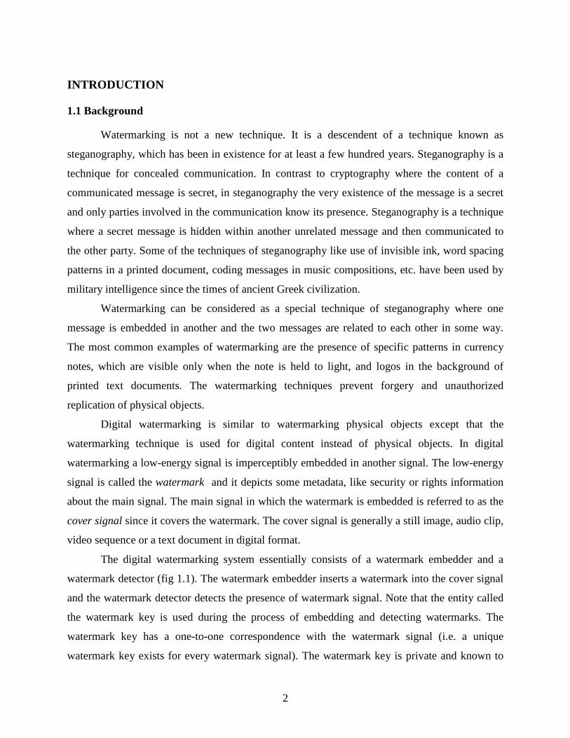
2.3 Classifications of Digital Watermarking Techniques
There are many watermark techniques in terms of their application areas and purposes.
And they have different insertion and extraction techniques. In this section we have discussed
some of the classification given by:
CLASSIFICATION CONTENT
Inserted media category Text, image, audio, video
Perceptivity of watermark Visible, invisible
Robustness of watermark Robust, semi-fragile, fragile
Inserting watermark type Noise, Image format
Spatial domain LSB, Random function Processing method
Transform domain Look-up table, spread spectrum
Necessary data for extraction Private, semi-private, public watermarking
Table 2.1: Classification of Watermarking according to several viewpoints
2.3.1 Classification according to inserted media
There have been many watermark researches for text and image so far, but video and
audio watermark are also required along with wide-spread internet applications.

9
Text watermarking: It inserts a watermark in the font shape and the space between character and
line spaces. This has some disadvantages as one cannot detect the watermark in case of
modulating the font.
Image watermarking: This embeds special information and detects or extracts it later for
ownership information. This approach is most widely
• Video watermarking: it is an extension of image watermarking. The method
requires real time extraction and robustness for compression.
• Audio watermarking: this application area becomes a hot issue because of internet
music, MP3. This approach needs watermark approaches and inaudibility like
other cases.
2.3.2 Classification according to robustness, visibility and keys.
• Robust and Fragile watermarking: Robust watermarking is a technique in which
modification to the watermarked content will not affect the watermark. As opposed to this,
fragile watermarking is a technique in which watermark gets destroyed when watermarked
content is modified or tampered with.
• Visible and Transparent watermarking: Visible watermarks are one which are embedded in
visual content in such a way that they are visible when the content is viewed. Transparent
watermarks are imperceptible.
• Asymmetric & Symmetric watermarking: Asymmetric watermarking (also called
asymmetric key watermarking) is a technique where different keys are used for embedding and
detecting the watermark. In symmetric watermarking (also called symmetric key watermarking)
the same keys are used for embedding and detecting watermarks.
2.4 Frame work And Parameters
In order to identify important watermarking parameters and variables, we first need to
have a look at the generic watermarking embedding and recovery schemes
10
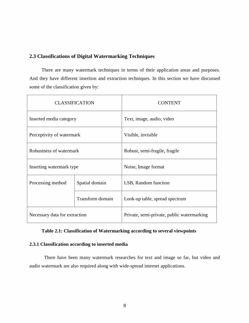
Fig.2.1 illustrates the embedding process. Given an image I, a watermark W and a key K
(usually the seed of a random number generator) the embedding process can be defined as a
mapping of the form: I*W*K I’ and is common to all watermarking methods.
The generic detecting process is depicted in Fig.2.2. Its output is either the recovered
watermark W or some confidence measure indicating how likely it is for a given watermark at
the input to be present in the image I’ under inspection.
Watermarked image (W)
Original image (I) watermarked image (I)
Secret public key (K)
Fig 2.1: Embedding Watermark
Watermark/image I
Test image (I’) watermark/confidence
Secret/public key (K)
Fig 2.2: Detecting Watermark
There are several types of watermarking systems. They are classified by their inputs and
outputs:
Private watermarking: systems require at least the original image. Type-1 systems extract the
watermark W from the possibly distorted image I’ and use the original image I as a hint to find
where the watermark could be in I’ i.e. I’*I*K W. Type-2 systems also require a copy of
the embedded watermark for extraction and just yield a ‘yes’ or a ‘no’ as to whether I’ contains
Digital watermarking
Watermark Decoder

11
W or not i.e. I’*I*K*W {0, 1}. This type of scheme is expected to be more robust since
it conveys very little information.
Semi-private watermarking: does not use the original image for detection but answers the
same question. The only use of private and semi-private watermarking seems to be evidence in
court to prove ownership and copy-control in applications such as DVD where the reader needs
to know whether it is allowed to play the content or not.
Public watermarking: remains the most challenging problem since it requires neither the secret
original I, nor the watermark W. Indeed such systems really extract n bits of information from
the watermarked image i.e. I*K W. Public watermarks have much more applications than
others and we have focused our work on these systems. Actually the embedding algorithms used
in public systems can always be used into a private one to improve robustness at the same time.
After grouping different systems, we can now identify different parameters and variables.
Amount of embedded information: This is an important parameter since it directly influences
the watermark robustness. The more information one wants to embed; the lower is the watermark
robustness. The information to be hidden depends on the application.
Watermark embedding strength: There is a tradeoff between the watermark embedding
strength and quality. Increased robustness requires stronger embedding, which in turn increases
the visual degradation of the image.
Size and nature of the image: Although very small pictures have very low commercial value,
watermarking technique needs to be able to recover a watermark from them. Photographers and
stock companies have great concerns about having their work stolen and most of them still rely
on small images, visible watermarks and even rollover java scripts to reduce infringement.
Secret information: although the amount of secret information has no direct impact on the
visual fidelity of the image or the robustness of the watermark, it plays an important role in the
security of the system. The key space i.e. the range of all possible values of the secret
information should be large enough to make exhaustive search attacks impossible.

12
Chapter 3
DIGITAL WATERMARKING TECHNIQUES
CLASSIFICATION
3.1 Techniques in Spatial domain
3.2 Techniques in Frequency domain
3.3 Experimental results
3.4 Conclusion
13
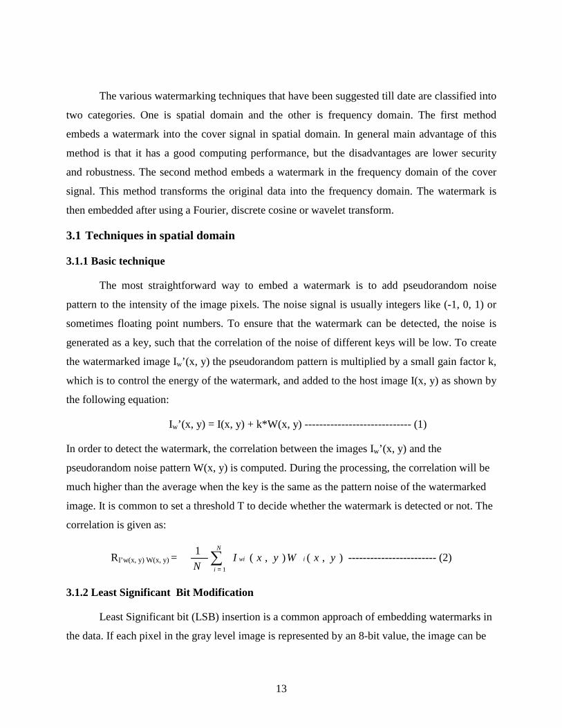
The various watermarking techniques that have been suggested till date are classified into
two categories. One is spatial domain and the other is frequency domain. The first method
embeds a watermark into the cover signal in spatial domain. In general main advantage of this
method is that it has a good computing performance, but the disadvantages are lower security
and robustness. The second method embeds a watermark in the frequency domain of the cover
signal. This method transforms the original data into the frequency domain. The watermark is
then embedded after using a Fourier, discrete cosine or wavelet transform.
3.1 Techniques in spatial domain
3.1.1 Basic technique
The most straightforward way to embed a watermark is to add pseudorandom noise
pattern to the intensity of the image pixels. The noise signal is usually integers like (-1, 0, 1) or
sometimes floating point numbers. To ensure that the watermark can be detected, the noise is
generated as a key, such that the correlation of the noise of different keys will be low. To create
the watermarked image Iw’(x, y) the pseudorandom pattern is multiplied by a small gain factor k,
which is to control the energy of the watermark, and added to the host image I(x, y) as shown by
the following equation:
Iw’(x, y) = I(x, y) + k*W(x, y) ----------------------------- (1)
In order to detect the watermark, the correlation between the images Iw’(x, y) and the
pseudorandom noise pattern W(x, y) is computed. During the processing, the correlation will be
much higher than the average when the key is the same as the pattern noise of the watermarked
image. It is common to set a threshold T to decide whether the watermark is detected or not. The
correlation is given as:
RI’w(x, y) W(x, y) = ),(),(1
1
yxWyxIN
i
N
i
wi∑=
------------------------ (2)
3.1.2 Least Significant Bit Modification
Least Significant bit (LSB) insertion is a common approach of embedding watermarks in
the data. If each pixel in the gray level image is represented by an 8-bit value, the image can be

14
spliced up into 8-bit planes. Since the least significant bit plane does not contain visually
significant information, it can easily be replaced by an enormous amount of watermark bits.
To hide the image in the LSBs of each byte of a 24-bit image, you can store 3 bits in each
pixel. A 1024×768 bit image has the potential to hide a total of 2,359,296 bits of information. If
you compress the watermark to be hidden before you embed it, you can hide a large amount of
information. To the human eye, the resulting watermarked image will look identical, to the
original image.
Example: The letter A can be hidden in 3 color pixels (assuming no compression). The original
raster data of the 3 pixels (9 bytes) may be:
(00100111 11101001 11001000)
(00100111 11001000 11101001)
(11001000 00100111 11101001)
The binary value of A is 10000011. Inserting the binary value for A in 3 pixels would result in:
(00100111 11101000 11001000)
(00100110 11001000 11101000)
(11001001 00100111 11101001)
The underlined bits are the only four actually changed in the 8 bytes used. On average,
LSB requires that only half the bits in an image be changed. You can hide data in the least and
second least significant bits and still the human eye would not be able to discern it.
The LSB insertion methods for watermarks is not very secure and robust to processing
techniques because the LSB plane can easily be replaced by random bits, effectively removing
the watermark bits. It is also vulnerable to slight image manipulations. Converting an image from
lossless compression to lossy compression and then back could also destroy the hidden
information.
3.2 Techniques in Frequency Domain
3.2.1Discrete cosine transform
The Discrete Cosine Transform (DCT) based watermarking scheme is a transform
domain algorithm for embedding watermarks into images. Normally the DCT is used for

15
decomposing the host image into parts (or spectral sub-bands) of differing importance while
taking the images visual quality into respect (Fig.3.1). The DCT transforms a signal or image
from spatial domain to the frequency domain.
Fig 3.1:Defination of DCT Regions
The middle band is chosen as the embedding region as to provide additional resistance to
lossy compression techniques, while avoiding significant modification of the cover image. A
basic scheme of the watermark embedding and detecting in DCT is given in Fig.3.2.
3.2.2 DCT Watermark casting
Discrete Cosine Transform uses the cosine transform to represent original data. The
watermark is cast by first computing the N×N DCT coefficient matrix of an N×N image. Where
A (i, j) is the intensity of the pixel in row I and column j. The DCT T(u, v) is calculated as:
T (u, v) =
+
+∑∑
−
=
−
= N
vj
N
uivujiA
N
j
N
i 2
)12(cos
2
)12(cos).()().,(
1
0
1
0
ππαα --------------- (3)
Where u, v = 0, 1, 2, 3………………….., N-1
α(u) = α(v) = (1/N)0.5 for u = 0
(2/N)0.5 for u = 1,2,…..N-1
The DCT coefficients are then reordered by the zigzag scan. For most images, much of
the signal energy lies at low frequencies; these appear in the upper left corner of the DCT. The
lower right values represent higher frequencies and are small enough to be neglected with little

16
visible distortion. The watermark is embedded by leaving the first L coefficients intact and only
changing the last M coefficients where L+M is the total number of coefficients.
Fig 3.2. DCT Based Watermark
Assume the first L+M DCT coefficients are:
is the pseudo-random watermark
After modifying the DCT coefficient we take the inverse DCT to get the watermark image.
The IDCT is defined as:
A (i, j) =
+
+∑∑
−
=
−
= N
vj
N
uivuvuT
N
j
N
i 2
)12(cos
2
)12(cos).()().,(
1
0
1
0
ππαα --------------- (4)

17
3.2.3 DCT Watermark Detection
In the detection process, given a corrupted image, the NxN DCT is computed, then re-
ordered by the zigzag scan. The L+1 to L+M coefficients are selected to form a vector T*. The
correlation of T* and the mark Y is calculated as:
----------------------------(5)
By comparing the correlation z to a pre-defined threshold, it is possible to determine if
the watermark exists or not.
Various studies have resulted in the prediction and minimization of the visual impact of
the distortion caused by the watermark. Lossy compression can be anticipated by embedding the
watermark in the same domain as the compression scheme used to process the image, thereby
making the watermark more robust.
3.3 Experimental Results
Both the algorithms are simulated using MATLAB 6.5 in a Pentium-IV processor (2.4 GHz).
In image processing techniques, Peak Signal to Noise Ratio (PSNR) is usually used to
assess the differences in the degree of image quality, from pre-processing to post-processing. A
large value of PSNR means there is little difference between original image and processed
image. A PSNR value greater than or equal to 30 means that the processed image quality is
acceptable.
The efficacy index, Bit Code Ratio (BCR) is defined as:
BCR = watermarkof size
original as recovered pixels ofNumber ---------------- (6)

18
The watermarked image is subjected to low pass filtering, high pass filtering, cropping, Gaussian
noise addition, salt and pepper noise addition and lossy compression. The retrieved watermarks
from these distorted images are recognizable in some cases.
Fig 3.3 Result Images of DCT Based Method
19
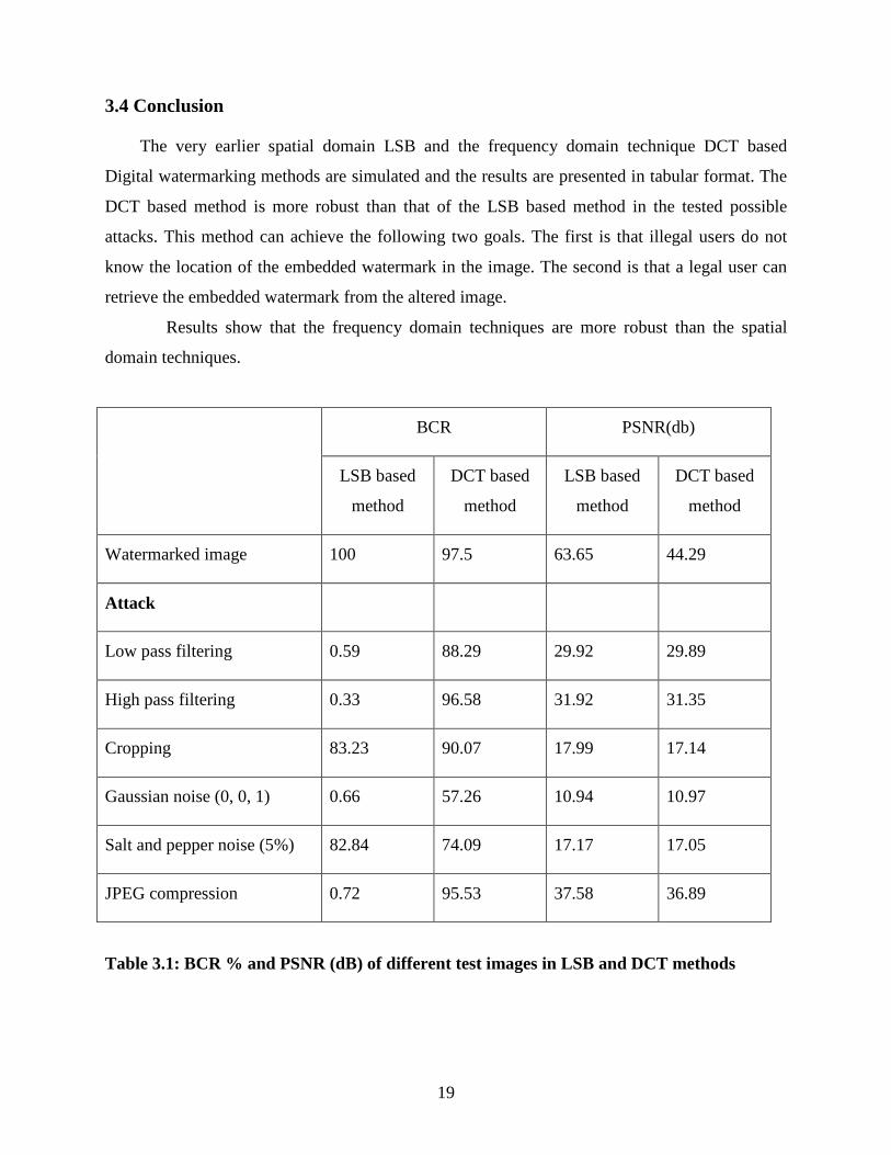
3.4 Conclusion
The very earlier spatial domain LSB and the frequency domain technique DCT based
Digital watermarking methods are simulated and the results are presented in tabular format. The
DCT based method is more robust than that of the LSB based method in the tested possible
attacks. This method can achieve the following two goals. The first is that illegal users do not
know the location of the embedded watermark in the image. The second is that a legal user can
retrieve the embedded watermark from the altered image.
Results show that the frequency domain techniques are more robust than the spatial
domain techniques.
BCR PSNR(db)
LSB based
method
DCT based
method
LSB based
method
DCT based
method
Watermarked image 100 97.5 63.65 44.29
Attack
Low pass filtering 0.59 88.29 29.92 29.89
High pass filtering 0.33 96.58 31.92 31.35
Cropping 83.23 90.07 17.99 17.14
Gaussian noise (0, 0, 1) 0.66 57.26 10.94 10.97
Salt and pepper noise (5%) 82.84 74.09 17.17 17.05
JPEG compression 0.72 95.53 37.58 36.89
Table 3.1: BCR % and PSNR (dB) of different test images in LSB and DCT methods

20
Chapter 4
DIGITAL WATERMARKING USING
NEURAL NETWORKS
4.1 Watermarking using Back Propagation Network
4.2 Proposed method using RBFNN
4.3 Experimental Results
4.4 Discussion
4.5 Conclusion

21
A neural network is a potential tool in most of the signal processing and other
application. Digital watermarking is not an exception where it finds a way to use neural network
in order to make the process more secure and robust. Different models of neural network have
their own merits and demerits. A BPN and DCT based watermarking is described below and
subsequently a modified RBFNN is suggested to gain in terms of computational efficiency as
well as memory requirements.
4.1 Watermarking using Back Propagation Network
In this section, brief discussion has been made on discrete cosine transform (DCT), the
concept of one-way hash functions and the Back Propagation Network (BPN). The scheme is
based on these foundations.
DCT can concentrate an image’s energy into the left-upper corner. According to this
characteristic, DCT has been used for image data compression, such as JPEG. Generally the
DCT blocks (8×8) are not overlapped in its applications. In this scheme the DCT blocks are
allowed to overlap partially. In this way, the security of the digital watermarking can be
improved. In other words, a pirate can not exactly obtain the DCT block in this scheme.
The concept of one way hash function involves providing an arbitrary parameter x to a
function h, which can easily produce an output value z=h(x). However, it is difficult to produce x
from the output value z. the characteristic of the one-way hash function is given x, it is difficult
to find other x’ such that h (x’) =h(x). To demonstrate the concept of one-way hash function, the
following sample example is provided. Let z=gx mod p, where g, x and p are 512 bits in length. It
is simple to produce z using exponential operation but very difficult to produce x from z.
There are many famous one-way hash functions that have been applied, such as MD5 and
SHA etc. In this scheme, a one-way hash function is used as given by Hwang to decide the
location of the DCT blocks in which the watermark is to be hidden.
The Back Propagation Network (BPN) is one type of supervised learning neural network.
It’s a very popular model in neural networks. The principle behind BPN involves using the
steepest gradient decent method to reach the smallest error tolerance.
The general model has architecture like depicted in Fig. 4.1. There are three types of
layers, input layer, hidden layer and output layer. Each layer has one or more neurons or units.
Each unit is fully connected to its adjacent layers or units. There may be more than one hidden
layer, according to practical necessity. Two units of each adjacent layer are directly connected to
each other called link. Each link has a weighted value, representing the relational degree between

22
the two units. Each input vector has its own mapping output vector in the BPN model. The
computing functions of units are shown in Fig. 4.2. The details of the training algorithm are
depicted below.
Fig 4.1 Architecture of a BPN network
Fig 4.2 Layout of a single neuron
netj (t) = ∑ +t
jiij tow θ)( ,
αj (t+1) = fact( netj (t) ), ---------------------------------------(7)
oj(t) = fout( αj( t) ) ,
Where
j = index of some current unit.
i = index of a predecessor of the current unit j.
αj (t) = activation of unit j in iteration t.
fact ( ) = activation function.
netj (t) = input value in unit j in iteration t.
23
jθ = threshold or bias of unit j.
ijw =weight of the link from unit I to unit j.
oj(t) = output of unit j in iteration t.
fout ( ) = output function.
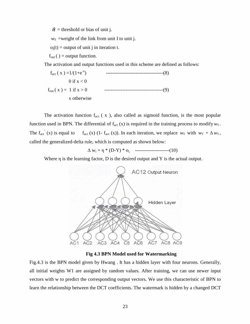
The activation and output functions used in this scheme are defined as follows:
fact ( x ) =1/(1+e-x) -----------------------------------(8)
0 if x < 0
fout ( x ) = 1 if x > 0 ------------------------------------(9)
x otherwise
The activation function fact ( x ), also called as sigmoid function, is the most popular
function used in BPN. The differential of fact (x) is required in the training process to modifyijw .
The fact’ (x) is equal to fact (x) (1- fact (x)). In each iteration, we replace ijw with ijw + ∆ ijw ,
called the generalized-delta rule, which is computed as shown below:
∆ wi = η * (D-Y) * o i, ---------------------(10)
Where η is the learning factor, D is the desired output and Y is the actual output.
Fig 4.3 BPN Model used for Watermarking
Fig.4.3 is the BPN model given by Hwang . It has a hidden layer with four neurons. Generally,
all initial weights W1 are assigned by random values. After training, we can use newer input
vectors with w to predict the corresponding output vectors. We use this characteristic of BPN to
learn the relationship between the DCT coefficients. The watermark is hidden by a changed DCT

24
coefficient, with one bit hidden in each DCT block. Since the relationship is recorded by whole
weight and threshold values. We can retrieve the approximate original coefficients using these
weights and thresholds. The watermark can be retrieved using changed coefficients and
approximate original coefficient .
4.1.1 Watermark Embedding
1. After obtaining the DCT block for an image choose the first 9 coefficients (AC1-AC9) as
the input vector and desired output as the AC12 for the ith DCT block.
2. The inputs are expanded by the sigmoid function Fact.
3. Train the block using the BPN model until the MSE is minimum or constant.
4. Embed the binary watermark Wi by replacing the original AC12i with AC12i’ where
AC12i – δ if Wi = 0
AC12i =
AC12i + δ if Wi = 1
5. Repeat step 4 till all the bits of the watermark are embedded.
6. Take the inverse DCT to obtain the watermarked image.
4.1.2 Extracting the Watermark
1. Introduce the secret keys to obtain the DCT blocks.
2. Use the AC1,AC2…..AC9 coefficients of the ith block as the inputs for the BPN
architecture to get the observed AC12i and then retrieve the watermark using
W’i = 0 if AC12i <= AC12’i
1 if AC12i > AC12’i
3. Compare the original watermark W and the extracted W’i.
4.1.3 Simulation Results
Fig 4.4 shows the training process for the original lena image by using BPN model until the
deserved goal is met. And the figures shown below are the simulated results of the watermarked

25
image on different type of attacks. The PSNR and the BCR values for these simulated results is
shown in Table 3.
Fig 4.4 Result Images of BPN-DCT Based Method

26
4.2 Proposed Method using RBFNN
In this thesis; we have proposed a digital watermarking scheme, which embeds the watermark
into the frequency domain. In this scheme, we have used a Radial Basis Function Neural
Network (RBFNN) to improve both security and robustness of the watermarked image. A one-
way hash function is also used n this scheme to decide the locations of the embedded watermark
for enhancing security.
4.2.1 Radial Basis Function Neural Network (RBFNN)
The RBF network is a popular alternative to the MLP which, although it is not as well suited to
larger applications, can offer advantages over the MLP in some applications. An RBF network
can be easier to train than an MLP network. The main advantage of the RBFNN is the reduced
computational cost in the training stage, while maintaining a good performance of
approximation. Also less number of weights is required to store or less memory requirement for
the verification or testing in a later stage.
Radial-Basis Function Networks used for pattern classification are based on Cover’s
theorem on the separability of patterns. This theorem states that nonlinearly separable patterns
can be separated linearly if the pattern is cast nonlinearly into a higher dimensional space.
Therefore we are looking for a network that converts the input to a higher dimension after which
it can the classified using only one layer of neurons with linear activation functions.
That’s why the structure of a RBFN is simple. It contains an input layer, a hidden layer
with nonlinear activation functions and an output layer with linear activation functions. Fig-4.5
shows the architecture of a RBFNN.

27
Fig 4.5 Radial Basis Neural Network Architecture
The RBF network has a similar form to the MLP in that it is a multi-layer, feed-forward
network. However, unlike the MLP, the hidden units in the RBF are different from the units in
the input and output layers: they contain the “Radial Basis Function”, a statistical transformation
based on a Gaussian distribution from which the neural network’s name is derived. Like MLP
neural networks, RBF networks are suited to applications such as pattern discrimination and
classification, pattern recognition, interpolation, prediction and forecasting, and process
modeling.
In the hidden layer of an RBF, each hidden unit takes as its input all the outputs of the input
layer x,. The hidden unit contains a “basis function” which has the parameters “center” and
“width”. The center of the basis function is a vector of numbers c1 of the same size as the inputs
to the unit and there is normally a different center for each unit in the neural network. The first
computation performed by the unit is to compute the “radial distance”, d, between the input
vector xi and the center of the basis function, typically using Euclidean distance:
d= ))(.......)22()11(( 222 cnxncxcx −++−+−
The unit output a is then computed by applying the basis function B to this distance divided by
the width o:
v=B ( )σd

28
The basis function is a curve (typically a Gaussian function), which has a peak at zero
distance, and which falls to smaller values as the distance from the center increases. As a result,
the unit gives an output of one when the input is “centered” but which reduces as the input
becomes more distant from the center. There are three sets of variables that affect each nodes
input to the solution, the position, the width and the output layer weight.
Several widely used basis functions are:
multiquadratics: )()( 22 cxx +=φ for some c>0
inverse multiquadratics: )(xφ =1/ )( 22 cx + for some c>0
Gaussian: )(xφ =exp (-x²/2σ²) for some σ>0
Multivariate Gaussian: )(xφ = exp(-║x-ci║2/2σ²) for some σ>0
—
The multivariate Gaussian function provides two important properties that make it a proper
choice for building radial-basis functions: it is both translation and rotation invariant.
The output node is a linear node as described in the MLP with a linear summation of the
weights and the outputs from the hidden Gaussian neurons
represented as yj = ∑=
+n
i
iji xw1
)( θφ ----------------------------- (11)
Where w is the weight from the i th hidden neuron to the output neuron and Ө is the bias value to
the jth output neuron.
A flat network results for which only the connection weights and the bias term must be learned.
Thus the back-propagation learning algorithm, used for adapting the RBFNN’s parameters,
becomes very simple
Back Propagation Training using LMS algorithm:
The optimization of the cost function of the RBFNN can be done by Gradient Descent technique
by taking the partial derivative of the cost function with respect to each of the parameter of the
RBFNN. The parameters of RBFNN include the centers, the variance of the hidden nodes and

29
the weights of the connecting path of the neural network. The training algorithm is derived as
follows:
Let the error vector at the output unit is e = (d — y), where d= desired output vector and
y =estimated output vector. Let E denotes half of the square error vector and is considered as the
cost function. Taking the partial derivative of E with respect to different network parameters the
update equations for the center and width of the Gaussian function as well as the connecting and
bias weights can be derived. The key equations obtained from the derivation are:
∆wji = n1eфi(x, c) ------------------------------------ (12)
∆ci = n2ewi ),(2
cxcx
ii φ
σ−
and ∆σi = n2ewi ),()(
3
2
cxcx
ii φ
σ− ----------------------- (13)
Where n1, n2, n3 are the learning parameters.
By applying each input pattern the change in the center location, width of the Gaussian
function as well as the connecting and bias weights are computed After all the patterns are
applied, the average change of different parameters is calculated and different network
parameters are updated once in each experiment, The update equation of the center position is
given by
ci (n + 1) = ci (n) + )(1
1
ncT
T
ti∑
=
∆ -------------------------------------(14)
Similarly the update equations for other parameters at (n+1) th iteration are given by
σk (n + 1) = σk (n) + )(1
1
nT
T
tk∑
=
∆σ ------------------------------------- (15)
wji (n + 1) = wji (n) + )(1
1
nwT
T
tji∑
=
∆ ------------------------------------- (16)
The main advantage of using RBFNN is that computational load is less compared to BPN
and less number of weights are required at the time of testing the watermarked image.
In this scheme, RBFNN is used to learn the relationship between the DCT coefficients.
The watermark is hidden by changing one of DCT coefficients. That is one bit of watermark is
hidden in one DCT block. Since the relationship is trained before the coefficient is changed, that
relationship is recorded using whole weights and threshold values. We can retrieve the
30
approximate original coefficients using these weights and thresholds. The watermark can be
retrieved by the relationship between the changed coefficients and the approximate original
coefficients.
4.2.2 Watermarking algorithm using RBFNN
Embedding of the Watermark
Step: I
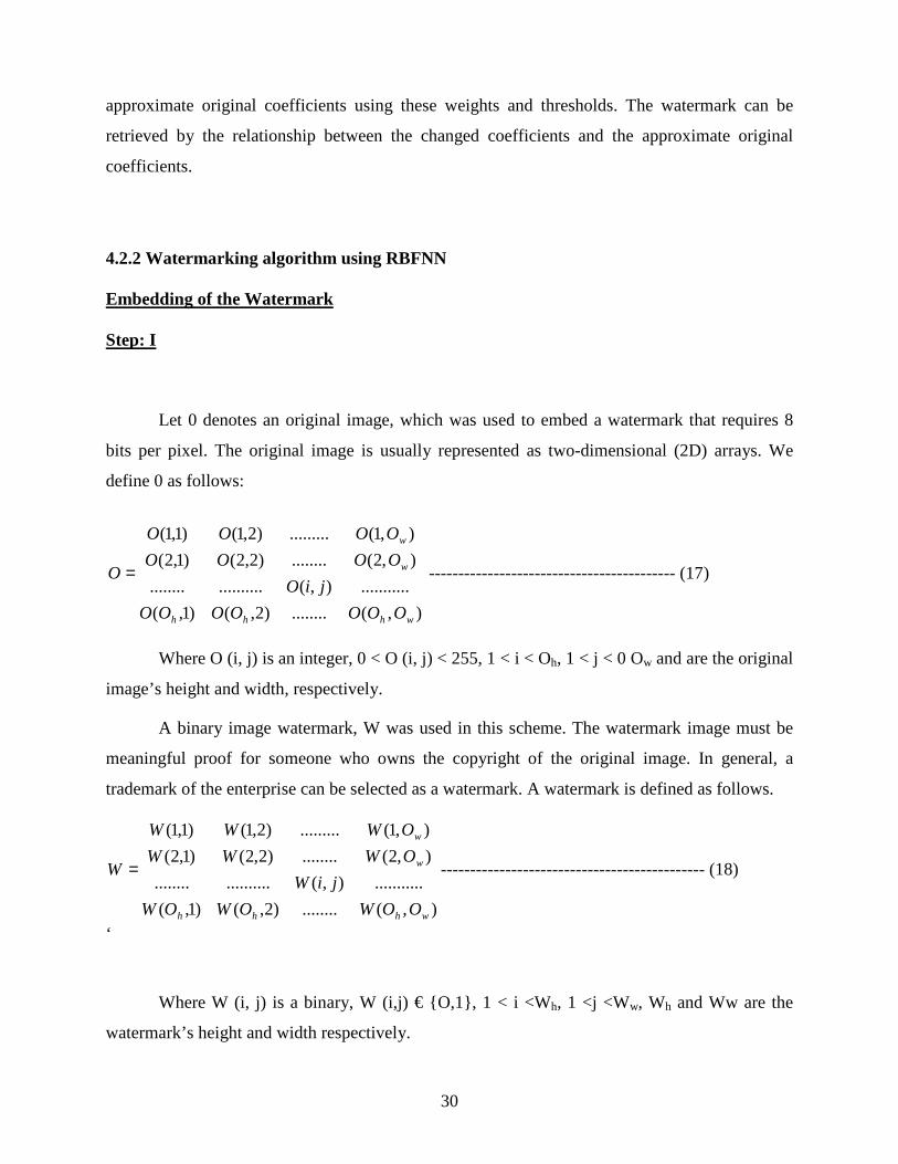
Let 0 denotes an original image, which was used to embed a watermark that requires 8
bits per pixel. The original image is usually represented as two-dimensional (2D) arrays. We
define 0 as follows:
),(........)2,()1,(
...........),(..................
),2(........)2,2()1,2(
),1(.........)2,1()1,1(
whhh
w
w
OOOOOOO
jiO
OOOO
OOOO
O = ------------------------------------------ (17)
Where O (i, j) is an integer, 0 < O (i, j) < 255, 1 < i < Oh, 1 < j < 0 Ow and are the original
image’s height and width, respectively.
A binary image watermark, W was used in this scheme. The watermark image must be
meaningful proof for someone who owns the copyright of the original image. In general, a
trademark of the enterprise can be selected as a watermark. A watermark is defined as follows.
),(........)2,()1,(
...........),(..................
),2(........)2,2()1,2(
),1(.........)2,1()1,1(
whhh
w
w
OOWOWOW
jiW
OWWW
OWWW
W = --------------------------------------------- (18)
‘
Where W (i, j) is a binary, W (i,j) € {O,1}, 1 < i <Wh, 1 <j <Ww, Wh and Ww are the
watermark’s height and width respectively.

31
The watermark is represented as 2D arrays. In order to hide the watermark in the original
image, we converted the stored 2D data into a one-dimensional array as follows.
W= (W1 … Wk………….. WhxWw), Step: 2
Let two prime numbers, p and q are chosen, and let n be equal to the product of p and q.
Two secret keys k1 and k2 are chosen by the images owner, which are used to decide the
locations (x1 y1) where the watermark will be hidden. (xi, yi) is computed using the following
location decision procedure.
1. Compute the initial location (Xi, Yi) as follows.
X1 = k12 mod n, Y1= k2
2 mod n, x1 = X1 mod O,,, y1 = Y1 mod Oh.
2. Compute the other ( Wh x Ww) -1 locations as follows Xi= X1i-1 mod n, Yi = Yi-1 mod n, x1 = X1 mod Ow, y1 = Y1 mod Oh, ---------------(19) Where i= 2,…………………… (Wh x Ww). Using the same location must be avoided. In other words, If (xi, yi) have been chosen in this procedure, ignore the (xi, yi) location. After this step, we get Wh x Ww., locations (xi, yi) These location are different from (x1,y1) and each other. Therefore, using the location decision procedure, we can produce Wh X Ww available locations in total. Each location corresponds to a sub image Mi. Here Mi is produced using:
M i = Sub matrix (0, x, x1+7, y, y1+7), 1 <i <Wh X Ww,
Where the function sub matrix (.) denote acquiring a DCT block from the image 0’s coordinate
(xi, yi) to coordinate (xi+7, yi+7). Maybe these blocks are partially overlapped (Fig.4.6). Next we
make these Mi, to perform the DCT transformation.

32
Fig 4.6 Selected overlapped DCT blocks
Step: 3
Choose the first nine AC coefficients (AC1i, AC2i,. ,..,.AC9i) as the input vector and the
twelfth AC coefficient ACI2i is the output vector in the RBFNN model. The number of AC
coefficients is shown in Fig 4.7. Note that AC1O, AC1 1 .AC14 are also candidates for the
output vector. According to the DCT characteristic, as the AC number decreases, the robustness
of the watermark increases at the same time the quantity of the watermarked image is decreased.
Fig 4.7: Number of AC Components
The RBFNN model used in our scheme is shown in fig 4.8. We take 9 AC coefficients as input.

33
Fig 4.8
The initial weight wij and the threshold of RBFNN model are random values in this scheme.
Weights are updated in the training; all weights w can be used as a secret key. The corresponding
output vector AC12i’ is acquired AC12i as:
AC12i’ = netACl2
Here netAC12 is a function (i.e. tanh() defined in RBFNN model which outputs the value of node
ACI2
Step: 4
The watermark Wi is embedded by replacing the original AC12i with AC12i’, where AC12i’’ is
computed according to AC12i and Wi as follows.
AC12i’’ = AC12i’ – σ if W i = 0; ---------------------------(20)
AC12i’ + σ if W i =1.
Here σ is a system parameter and is a constant, generally. A larger will result in a greater
robustness in the watermarked image. But the distortion will be increased too. The value ö can be
determined by the applicant’s requirements.

34
Step: 5
After the twelfth coefficients are replaced and the inverse DCT is transformed, the embedding
process is completed and we get the watermarked image.
Extracting of the Watermark Step: 1
The retrieval procedure for the watermark from the watermarked image is similar to the
embedding procedure. When the correct secret keys and weights are introduced, the
corresponding AC12i and AC12i’, can be obtained.
Step: 2
The retrieved watermark is produced using the relationship between AC12i, and AC12i’ as
Wi’ = 0 if AC12i < AC12i’;
1 if AC12i > AC12i’. ------------- (21)
Step: 3
The similarity between the original watermark W and the extracted watermark W is
quantitatively measured by the bit correct ratio (BCR), defined as follows:
BCR = %100*'
1
wh
ww
iii
ww
wwwh
∗
⊗∑∗
= --------------------------------------- (22)
Where wi is the original watermark bit, wi’ is the extracted watermark bit, ⊗ denotes the
exclusive — OR operator.

35
4.3 Experimental Results
In image processing techniques, PSNR (Peak Signal to Noise Ratio) is usually used to
assess the differences in the degree of image quality, from preprocessing to post-processing. A
larger value of PSNR means there is a little difference between original image and processed
image. A PSNR value greater than or equal to 30 means that the processed image quality is
acceptable.
The algorithm is simulated using MATLAB 6.5 in a Pentium-IV processor (2.4GHz).
Lena image is chosen as the cover signal where a logo is used as watermark signal. The BPN and
RBFNN is trained using conventional back propagation algorithm and the saturated weights and
biases are used for retrieving the watermark from the watermarked image. Fig. 4.9 depicts the
MSE after 1000 epochs. In our experiment, we let σ is selected to be 20 and n1 = 0.2, n2=0.15
and n3=0.15. We can see from Fig.15 that RBFNN has faster convergence characteristics than
BPN and less Mean square Error.
Fig 4.9 Variations of the MSE (Mean Square Error)

36
The original image of “Lena” (512 x 512, 8 bits / pixel) is shown in Fig. 4.10. The watermark is
represented by (39 x 39) binary image. We used this scheme with the above parameter to embed
watermark into original image to produce the watermarked image. The PSNR of the
watermarked image is dB (using RBFNN). The retrieved watermark is shown in the figure. The
efficacy index, Bit Correct Ratio (BCR) defined as:
BCR = watermarkof size
original as recovered pixels ofNumber ---------------- (23)
The BCR in our case (RBFNN) is found to be 93.1%, which conveys the superiority of the
retrieval process over the BPN in which it is only 92.7%.
The watermarked image is subjected to low pass filtering, high pass filtering, Cropping,
Gaussian noise addition, salt and pepper noise addition and lossy compression. The retrieved
watermarks from these distorted images are recognizable in some cases. The retrieved
watermarks from these distorted images are recognizable. The results are shown in the Fig.4.10
Three methods are compared and the results the given in Table 4.1. First method is DCT-
based which is similar to BPN method, but does not use neural network. We have simulated the
DCT-based watermarking using logo as watermark. In this we have chosen the DCT blocks by
the hash function used in our algorithm. We just modify the ACI2 coefficient. From the table 4.1
we can see that its result is better than neural network method (BPN, RBFNN). But the
disadvantage is that it requires the original image at the time of testing.
The main advantage of the RBFNN over BPN is the reduced computational cost in the training
stage, while maintaining good performance of approximation. Also less number of weights is
required to store or less memory requirement for the verification or testing in a later stage.

37
Fig 4.10 Result Images of RBFNN-DCT Based Method
38
BCR PSNR (dB)
DCT BPN RBFNN DCT BPN RBFNN
Watermarked Image
97.5 92.70 93.10 44.29 38.10 39.74
Low pass filtering 88.29 62.19 69.29 29.89 31.21 31.28
High pass filtering 96.58 90.29 91.39 31.35 30.58 30.99
Cropping 90.07 84.28 84.35 17.14 13.38 13.38
Gaussian noise addition
57.26 60.62 54.96 10.97 10.98 10.99
Salt & Pepper noise addition
74.09 70.28 69.36 17.05 18.07 18.05
JPEG compression
95.53 90.14 91.43 36.89 34.96 34.29
Table 4.1: BCR % and PSNR (dB) of different test images of Lena in BPN and RBFNN methods
4.4 Discussion
The secret keys used in the neural network-based watermarking scheme anged from 0 to
n. The probability of directly destroying the Twelfth AC component of the watermarked image is
very low. The probability is
wh ww
wh OO
∗
∗1
-----------------------------------------(24)
Where Oh and Ow are the image’s height and width, and Wh and Ww are the watermark’s height
and width, respectively. Therefore the security of this scheme is very high.
39
The quality of the watermarked image is high (Fig.16(c)) in this scheme. In addition
original image is not needed in the procedure of retrieving the watermark. Consequently this
method has achieved the primary requirement for a reliable, high quality watermarking
technique.
Because we allow partially overlapped DCT blocks, the retrieved watermark from a non-
altered watermarked image has little noise. We can use non-overlapped DCT blocks to avoid this
phenomenon. But it will reduce the security at the same time and be vulnerable to attack. The
advantage of allowing partially overlapped DCT blocks is that there is no way to determine the
exact position of the DCT blocks except by the owner of the property. The DCT coefficients on
the left-upper corner suffered little change when the PSNR is larger than 30.
4.5 Conclusion
We have used Neural Networks and DCT for the digital watermarking of images. The
RBFNN was used to improve the robustness of the proposed scheme. This method can achieve
the following two goals. The first is that illegal users do not know the location of the embedded
watermark in the image. The second is that a legal user can retrieve the embedded watermark
from the altered (filtering, lossy compression,etc) image. We used RBFNN and DCT ,in which
blocks are allowed to partially overlap, to achieve this goal. The advantage of RBFNN over BPN
is that we require less weights (i.e. half of BPN) to store or memory requirements is less, also
less computation and has a good function approximation.

40
Chapter 5
CONCLUSION

41
5.1 Conclusion
In this thesis different existing digital watermarking methods are studied and attempts has
been made to improve their performance in terms of robustness, security features and
computational overhead. Exhaustive simulation has been done and results obtained thereof are
compared to evaluate the performance of the proposed schemes.
5.2 Further Enhancements
In our proposed RBF model we are using the gradient decent training technique for updating
the various parameters of the network. But this back propagation learning based on gradient
decent technique is computationally expensive. Researchers have proved that training of RBF
Networks using the Extended Kalman Filtering is quicker while providing the performance at the
same level of index. Also new techniques can be applied to make the watermarking more robust.

42
REFERENCES
[1] Anderson, R.J. and Petitcolas, F.(1998) “On the Limits of Stenography.” IEEE
Journal of Selected Areas in Communications, vol. 16, Issue: 4, May, pp. 474 – 481.
[2] Katzenbeisser,S. and Petitcolas,F.(2000)“Information Hiding Techniques for
Stenography and Digital Watermarking”, Artech House, 2000, pp. 245 – 267.
[3] White Paper, “Digital Watermarking: A Technology Overview”,
http://www.wipro.com/dsp.
[4] Sin-Joo Lee, Sung-Hwan Jung (2001) “A survey of watermarking techniques applied
to multimedia Industrial Electronics”, Proceedings. ISIE 2001. IEEE International
Symposium on June, vol. 1, pp. 272 – 277.
[5] Elizabeth, F. and Matthew, M.(1999) “A Survey of Digital Watermarking”, February
25,pp. 127- 156.
[6] Schyndel, R. Tirkel, A. and Osborne, C. (1994) “A Digital Watermark”, Proc. IEEE
Int. Conf. on Image Processing, Nov , vol. II, pp. 86-90.
[7] Hwang, M.S. Chang, C. and Hwang, K. F.(2000) “Digital watermarking of images
using Neural Networks”, Journal of Electronic imaging, ,pp. 548-555.
[8] Zhang Zin-Ming, Li Rong-Yon, Wang Le, “Adaptive watermark scheme with RBF
neural networks”, IEEE Intl. Conf. Neural Networks & Signal Processing, pp. 1517-
1520.
[9] Gerhard C. Langelaar, Iwan Setywan, and Reginald L. Lagendijk, "Watermarking
Digital Image and Video Data", IEEE Signal Processing magazine, Sep.2000,pp.
1053-1078.
[10] Hartung, J. K. Su, and. Girod, B "Spread spectrum watermarking: Malicious attacks
and counterattacks", Proc. SPIE 3657: Security and Watermarking of Multimedia
Contents, San Jose, CA, January, 1999.

43
[11] George, M. Chouinard,Y. and Georganas, N. " Spread Spectrum Spatial and Spectral
Watermarking of for Images and Video", Proc. 1999 IEEE Can.Workshop in
Information Theory (CWIT'99), Kingston, Ont., June 1999.
[12] Chiou-Ting Hsu and Ja-Ling Wu, "Hidden Digital Watermarks in Images", IEEE
Trans. Image proc., Vol. 8, No.1, Jan. 1999.
[13] Kutter,M. and Petitcolas,F. "A fair benchmark for image watermarking systems",
proceedings of Electronic Imaging '99, Security and Watermarking of Multimedia
Contents, vol. 3657, pp. 226~239, San Jose, California, U.S.A., January 1999.
[14] Cox, I. J. Kilian, J. .Leighton, F.T and Shamoon, T. "Secure Spread Spectrum
Watermarking for Multimedia", IEEE Trans. Image Proc., Vol. 6, No. 12, Dec. 1997.
[15] Jain, A.K. "Fundamentals of Digital Image Processing", Englewood Cliffs, NJ:
Prentice Hall, 1989, pp. 215 – 296.
[16] Yeung, M.M and Mintzer, F. "An Invisible Watermarking Technique for Image
Verification," Proceedings of IEEE ICIP'97, Santa Barbara, CA, Oct. 1997.
[17] Craver,S. Memon,N. Yeo, B.L and Yeung, M.M "Resolving Rightful Ownership
with Invisible Watermarking Techniques: Limitations, Attacks and Implications,"
IEEE JSAC, March 1997.
[18] Mintzer, F. Braudaway, G.B and Yeung, M.M. "Effective and Ineffective Digital
Watermarks," Proceedings of IEEE ICIP'97, Santa Barbara, CA, Oct. 1997.
[19] Berghel, H. "Watermarking Cyberspace", Communications of the ACM, Vol. 40, No.
11, November 1997.
[20] Van den Bergh, F. Engelbrecht, A. "Cooperative Learning in Neural Networks ".
CIRG 2000,pp. 26-67.