improved algorithms for the minmax-regret 1-center and 1-median problems

36

Improved Algorithms for the Minmax-Regret 1-Centerand 1-Median Problems

HUNG-I. YU, TZU-CHIN LIN, AND BIING-FENG WANG

National Tsing Hua University

Abstract. In this article, efficient algorithms are presented for the minmax-regret 1-center and 1-

median problems on a general graph and a tree with uncertain vertex weights. For the minmax-regret

1-center problem on a general graph, we improve the previous upper bound from O(mn2 log n) to

O(mn log n). For the problem on a tree, we improve the upper bound from O(n2) to O(n log2 n). For

the minmax-regret 1-median problem on a general graph, we improve the upper bound from O(mn2

log n) to O(mn2 + n3 log n). For the problem on a tree, we improve the upper bound from O(nlog2 n) to O(n log n).

Categories and Subject Descriptors: G.2.2 [Discrete Mathematics]: Graph Theory—Graph algo-rithms, trees

General Terms: Algorithms

Additional Key Words and Phrases: Location theory, minmax-regret optimization, centers, medians,

general graphs, trees

ACM Reference Format:Yu, H.-I., Lin, T.-C., and Wang, B.-F. 2008. Improved algorithms for the minmax-regret 1-center

and 1-median problems. ACM Trans. Algor. 4, 3, Article 36 (June 2008), 27 pages. DOI =10.1145/1367064.1367076 http://doi.acm.org/10.1145/1367064.1367076

1. Introduction

Over three decades, location problems on networks have received much attention

from researchers in the fields of transportation and communication [Goldman 1971;

Preliminary versions of this article were published in Proceedings of the 12th Annual Interna-tional Computing and Combinatorics Conference (COCOON), Lecture Notes in Computer Science,

vol. 4112, Springer-Verlag, New York, 52–62, and the Proceedings of the 17th International Sym-posium on Algorithms and Computation (ISAAC), Lecture Notes in Computer Science, vol. 4288,

Springer-Verlag, New York, 537–546.

This research is supported by the National Science Council of the Republic of China under grants

NSC-94-2213-E-007-082 and NSC-95-2221-E-007-028.

Authors’ address: National Tsing Hua University, Hsinchu, Taiwan 30043, Republic of China, e-mail:

{herbert, rems, bfwang}@cs.nthu.edu.tw.

Permission to make digital or hard copies of part or all of this work for personal or classroom use is

granted without fee provided that copies are not made or distributed for profit or direct commercial

advantage and that copies show this notice on the first page or initial screen of a display along with the

full citation. Copyrights for components of this work owned by others than ACM must be honored.

Abstracting with credit is permitted. To copy otherwise, to republish, to post on servers, to redistribute

to lists, or to use any component of this work in other works requires prior specific permission and/or

a fee. Permissions may be requested from Publications Dept., ACM, Inc., 2 Penn Plaza, Suite 701,

New York, NY 10121-0701 USA, fax +1 (212) 869-0481, or [email protected]© 2008 ACM 1549-6325/2008/06-ART36 $5.00 DOI 10.1145/1367064.1367076 http://doi.acm.org/

10.1145/1367064.1367076

ACM Transactions on Algorithms, Vol. 4, No. 3, Article 36, Publication date: June 2008.

36:2 H.-I. YU ET AL.

Hakimi 1964; Kariv and Hakimi 1979a, 1979b; Ku et al. 2001; Megiddo 1983].

Traditionally, network location theory has been concerned with networks in which

the vertex weights and edge lengths are known precisely. However, in practice, it

is often impossible to make an accurate estimate of all these parameters [Kouvelis

et al. 1994; Kouvelis and Yu 1997; Nikulin 2004]. Real-life data often involve

a significant portion of uncertainty, and these parameters may change with the

time. Thus, location models involving uncertainty have attracted increasing research

efforts in recent years.

Several ways for modeling network uncertainty have been defined and studied.

One direction is the sensitivity analysis, which concerns the relationship between the

degree of change in parameters and the degree of change in the optimal objective

function value. On this model, Drezner [1980] studied the Euclidean minisum

problem and Labbe et al. [1991] discussed the minisum location problem on a tree

and on a plane using block norms. For a brief review of related literature, see Labbe

et al. [1991]. Another direction is the stochastic approach, in which parameters are

assumed to be stochastic with some known probabilistic distribution. Assuming

normally distributed vertex weights, Frank [1966, 1967] studied the 1-center and

the 1-median problems on a general graph. Assuming that both the vertex weights

and edge lengths are stochastic, Mirchandani and Odoni [1979] studied properties of

the p-median problem on a general graph. Later, Oudjit [1981], Weaver and Church

[1983], and Mirchandani et al. [1985] proposed implicit enumeration algorithms

for finding a solution.

In some practical situations, it is inappropriate to characterize uncertainty by any

specified probabilistic distribution. Kouvelis et al. [1994] pointed out that this could

indeed happen in the location-decision environment, and introduced the minmax-regret approach. In the approach, uncertainty of network parameters is character-

ized by given intervals, and it is required to minimize the worst-case loss in the

objective function that may occur because of the uncertain parameters. During the

last ten years, many researchers have concentrated on minmax-regret optimization

in various fields. A comprehensive treatment of the state of art in minmax-regret

optimization can be found in Kouvelis and Yu [1997] and Nikulin [2004], in which

various application areas are discussed, including scheduling, production planning,

assignment, resource allocation, etc. On the minmax-regret model, the 1-center

problem was studied in Averbakh and Berman [1997, 2000a] and Burkard and

Dollani [2002], the p-center problem was studied in Averbakh and Berman [1997]

and Averbakh [2000], and the 1-median problem was studied in Averbakh and

Berman [2000b, 2003], Brodal et al. [2008], Chen and Lin [1998], Kouvelis et al.

[1994] and Kouvelis and Yu [1997]. Recently, the minmax-regret 1-center and

1-median problems were studied on the plane in Averbakh and Bereg [2005].

The minmax-regret 1-center and 1-median problems are the focus of this article.

For a general graph with uncertain edge lengths, the minmax-regret 1-center prob-

lem is strongly NP-hard [Averbakh 2003]. For a general graph with uncertain vertex

weights, Averbakh and Berman [1997] gave an O(mn2 log n)-time algorithm, where

n is the number of vertices and m is the number of edges. For a tree with uncertain

vertex weights, the time complexity of their algorithm becomes O(n2) [Averbakh

and Berman 1997, 2000a]. For a tree with uncertainty in both vertex weights and

edge lengths, Averbakh and Berman [2000a] presented an O(n6)-time algorithm

and Burkard and Dollani [2002] had an O(n3 log n)-time algorithm. For a tree with

uncertain edge lengths, assuming uniform vertex weights, Averbakh and Berman


Improved Algorithms for Minmax and Median Problems 36:3

[2000a] presented an O(n2 log n)-time algorithm and Burkard and Dollani [2002]

had an (n log n)-time algorithm. In this paper, efficient algorithms are presented for

the minmax-regret 1-center problem on a general graph and a tree with uncertain

vertex weights. For general graphs, we improve the upper bound from O(mn2 log

n) to O(mn log n). For trees, we improve the upper bound from O(n2) to O(nlog2 n).

For a general graph with uncertain edge lengths, the minmax-regret 1-median

problem is also strongly NP-hard [Averbakh 2003]. For a general graph with un-

certain vertex weights, Averbakh and Berman [2000b] gave an O(mn2 log n)-time

algorithm. As to a tree, it was proved [Chen and Lin 1998] that uncertainty in

edge lengths can be ignored by setting the length of each edge to its upper bound.

For a tree with uncertain vertex weights, Kouvelis et al. [1994] first proposed an

O(n4)-time algorithm. Chen and Lin [1998] improved the bound to O(n3). Aver-

bakh and Berman [2000b] presented an O(n2)-time algorithm and then improved

it to O(n log2 n) in Averbakh and Berman [2003]. In this article, efficient algo-

rithms are also presented for the minmax-regret 1-median problem on a general

graph and a tree with uncertain vertex weights. For general graphs, we improve

the upper bound from O(mn2 log n) to O(mn2 + n3 log n). For trees, we im-

prove the upper bound from O(n log2 n) to O(n log n). We remark that very

recently, an O(n log n)-time algorithm for the minmax-regret 1-median problem

on a tree was independently obtained using a different approach in Brodal et al.

[2008].

The remainder of this article is organized as follows: In Section 2, notation and

definitions are given. In Sections 3 and 4, improved algorithms for the minmax-

regret 1-center problem are presented. Then, in Sections 5 and 6, improved algo-

rithms for the minmax-regret 1-median problem are proposed. Finally, in Section 7,

we conclude this article.

2. Notation and Preliminaries

Let G = (V , E) be an undirected connected graph, where V is the vertex set and

E is the edge set. Let n = |V | and m = |E |. In this article, G also denotes the

set of all points of the graph. Thus, the notation x ∈ G means that x is a point

along any edge of G which may or may not be a vertex of G. Each edge e ∈ Ehas a nonnegative length. For any two points a, b ∈ G, let d(a, b) be the distance

of the shortest path between a and b. Suppose that the matrix of shortest distances

between vertices of G is given. Each vertex v ∈ V is associated with two positive

values w−v and w+

v , where w−v ≤ w+

v . The weight of each vertex v ∈ V can take

any value randomly from the interval [w−v ,w+

v ]. Let � be the Cartesian product of

intervals [w−v ,w+

v ], v ∈ V . Any element S ∈ � is called a scenario and represents

a feasible assignment of weights to the vertices of G. For any scenario S ∈ � and

any vertex v ∈ V , let w Sv be the weight of v under the scenario S.

Let F(S, x) be a function that maps any scenario S ∈ � and point x ∈ G to a

real number. We discuss both center and median problems. For center problems,

F(S, x) = maxv∈V {w Sv × d(v , x)}, which is the maximum weighted distance from

any vertex in V to x according to S, and the point x ∈ G that minimizes F(S,

x) is called a classical 1-center of G under the scenario S. For median problems,

F(S, x) = ∑v∈V {w S

v × d(v , x)}, which is the total weighted distance from all the



(a) G

i

j kj' k'

i'

+− ii wSFM /))(( *

i

j k

(b) G'

FIG. 1. G and G ′.

vertices to x according to S, and the point x ∈ G that minimizes F(S, x) is called a

classical 1-median of G under the scenario S. For any point x ∈ G, the regret of xwith respect to a scenario S ∈ � is maxy∈G{F(S, x) − F(S, y)} and the maximumregret of x is

Z (x) = maxS∈�

maxy∈G

{F(S, x) − F(S, y)}.

When F(S, x) = maxv∈V {w Sv ×d(v , x)}, the finding of a point x that minimizes Z (x)

is called the minmax-regret 1-center problem. When F(S, x) = ∑v∈V {w S

v × d(v ,

x)}, the finding is called the minmax-regret 1-median problem.

3. The Minmax-Regret 1-Center Problem on a General Graph

Averbakh and Berman [1997] had an O(mn2 log n)-time algorithm for finding a

minmax-regret 1-center of a graph G = (V , E). Their algorithm is firstly described

in Section 3.1. Then, our improved algorithm is presented in Section 3.2.

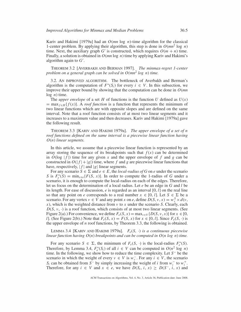
3.1. AVERBAKH AND BERMAN’S ALGORITHM. Averbakh and Berman [1997]

had an approach that solves the minmax-regret p-center problem by a reduction

to the classical p-center problem. Their approach can be viewed as an application

of the general methodology developed in Averbakh [2000], which allows reducing

a minmax-regret version of a problem to its classical version for a broad class of

problems with objective functions of a minmax type. For p = 1, Averbakh and

Berman’s reduction is described as follows. For any scenario S ∈ �, the 1-radiusof G under the scenario S is F∗(S) = minx∈G{F(S, x)}. For each i ∈ V , let Si be

the scenario in which the weight of i is w+i and the weight of any other vertex v is

w−v . Define an auxiliary graph G ′as follows: Let M = (maxv∈V w+

v ) × ∑e∈El(e),

where l(e) is the length of e. The graph G ′ is obtained from G by adding for each

i ∈ V a vertex i ′ and a dummy edge (i , i ′) with length (M − F∗(Si ))/w+i . (See

Figure 1.) Specific weights are assigned to the vertices of G ′. For each i ∈ V , the

weight of i is zero and the weight of i ′ is w+i . Averbakh and Berman [1997] gave

the following important property for solving the minmax-regret 1-center problem.

LEMMA 3.1 [AVERBAKH AND BERMAN 1997]. Let x∗ be a classical 1-centerof G ′. If x∗ is on a dummy edge (i , i ′), let x ′ = i ; otherwise, let x ′ = x∗. Then, x ′is a minmax-regret 1-center of G.

Based upon Lemma 3.1, Averbakh and Berman [1997] solved the minmax-regret

1-center problem as follows. First, for each i ∈ V , the 1-radius F∗(Si ) is computed.



Kariv and Hakimi [1979a] had an O(mn log n)-time algorithm for the classical

1-center problem. By applying their algorithm, this step is done in O(mn2 log n)

time. Next, the auxiliary graph G ′ is constructed, which requires O(m + n) time.

Finally, a solution is obtained in O(mn log n) time by applying Kariv and Hakimi’s

algorithm again to G ′.

THEOREM 3.2 [AVERBAKH AND BERMAN 1997]. The minmax-regret 1-centerproblem on a general graph can be solved in O(mn2 log n) time.

3.2. AN IMPROVED ALGORITHM. The bottleneck of Averbakh and Berman’s

algorithm is the computation of F∗(Si ) for every i ∈ V . In this subsection, we

improve their upper bound by showing that the computation can be done in O(mnlog n) time.

The upper envelope of a set H of functions is the function U defined as U (x)

= max f ∈H { f (x)}. A roof function is a function that represents the minimum of

two linear functions which are with opposite slopes and are defined on the same

interval. Note that a roof function consists of at most two linear segments and it

increases to a maximum value and then decreases. Kariv and Hakimi [1979a] gave

the following result.

THEOREM 3.3 [KARIV AND HAKIMI 1979a]. The upper envelope of a set of nroof functions defined on the same interval is a piecewise linear function havingO(n) linear segments.

In this article, we assume that a piecewise linear function is represented by an

array storing the sequence of its breakpoints such that f (x) can be determined

in O(log | f |) time for any given x and the upper envelope of f and g can be

constructed in O(| f |+ |g|) time, where f and g are piecewise linear functions that

have, respectively, | f | and |g| linear segments.

For any scenario S ∈ � and e ∈ E , the local-radius of G on e under the scenario

S is F∗e (S) = minx∈e{F(S, x)}. In order to compute the 1-radius of G under a

scenario, it is enough to compute the local-radius on each of the edges. Therefore,

let us focus on the determination of a local radius. Let e be an edge in G and l be

its length. For ease of discussion, e is regarded as an interval [0, l] on the real line

so that any point on e corresponds to a real number x ∈ [0, l]. Let S ∈ � be a

scenario. For any vertex v ∈ V and any point x on e, define D(S, v , x) = w Sv ×d(v ,

x), which is the weighted distance from v to x under the scenario S. Clearly, each

D(S, v , ·) is a roof function, which consists of at most two linear segments. (See

Figure 2(a).) For convenience, we define Fe(S, x) = maxv∈V {D(S, v , x)} for x ∈ [0,

l]. (See Figure 2(b).) Note that Fe(S, x) = F(S, x) for x ∈ [0, l]. Since Fe(S, ·) is

the upper envelope of n roof functions, by Theorem 3.3, the following is obtained.

LEMMA 3.4 [KARIV AND HAKIMI 1979a]. Fe(S, ·) is a continuous piecewiselinear function having O(n) breakpoints and can be computed in O(n log n) time.

For any scenario S ∈ �, the minimum of Fe(S, ·) is the local-radius F∗e (S).

Therefore, by Lemma 3.4, F∗e (Si ) of all i ∈ V can be computed in O(n2 log n)

time. In the following, we show how to reduce the time complexity. Let S− be the

scenario in which the weight of every v ∈ V is w−v . For any i ∈ V , the scenario

Si can be obtained from S− by simply increasing the weight of i from w−i to w+

i .

Therefore, for any i ∈ V and x ∈ e, we have D(Si , i , x) ≥ D(S−, i , x) and



(a) Three cases of D(S, v, x).

(b) Fe (S, x).

0 l

Fe(S, x)

x

0 l

x

0 l

x

0 l

x

FIG. 2. D(S, v , x) and Fe(S, x).

(a) Fe(S−, x) and D(Si, i, x). (b) Fe(Si, x).

Fe(Si, x)

0 l

D(Si, i, x)

Fe(S–, x)

0 l

FIG. 3. An illustration for Lemma 3.5.

D(Si , v , x) = D(S−, v , x) for all v �= i . Consequently, the following relation

between Fe(Si , ·) and Fe(S−, ·) is established. (See Figure 3.)

LEMMA 3.5. For any i ∈ V and x ∈ e, Fe(Si , x) = max{Fe(S−, x), D(Si , i ,x)}.

According to Lemma 3.5, Fe(Si , ·) is the upper envelope of Fe(S−, ·) and D(Si ,

i , ·). Since Fe(S−, ·) contains O(n) linear segments and D(Si , i , ·) contains at

most two linear segments, it is easy to compute their upper envelope in O(n) time.



(a) r lies on the left boundary of R.

(b) r does not lie on the left boundary of R.

r

0 lxr

left boundary

right boundary

r

lxr = 0

FIG. 4. An illustration for Lemma 3.7, in which solid lines represent R and dash lines represent A.

Therefore, after Fe(S−, ·) is determined, the time for computing each F∗e (Si ) can

be reduced to O(n). With some preprocessing on Fe(S−, ·), the time for computing

each F∗e (Si ) can be further reduced to O(log n). The trick is not to construct the

whole function Fe(Si , ·), but only to determine its minimum from Fe(S−, ·) and

D(Si , i , ·). For convenience, we define the radius-adjustment problem as follows.

Let R be a continuous piecewise linear function that has O(n) breakpoints and is

defined on an interval I = [0, l]. The radius-adjustment problem is to preprocess

R so as to answer the following queries efficiently: given a roof function A defined

on I , determine the minimum of max{R(x), A(x)} over all x ∈ I . Later, we will

present an efficient algorithm for the radius-adjustment problem. The presented

algorithm requires O(n) preprocessing time and O(log n) query time. Such a

result immediately leads to a procedure to compute F∗e (Si ) for every i ∈ V in O(n

log n) time. Consequently, we have the following theorem.

THEOREM 3.6. The minmax-regret 1-center problem on a general graph canbe solved in O(mn log n) time.

In the remainder of this section, we complete the proof of Theorem 3.6 by

presenting an efficient algorithm for the radius-adjustment problem. Since the query

function A is a roof function, it consists of at most two linear segments. In the

following, we first discuss the case that A contains only a linear segment with

positive slope. Two vertical linear segments are associated with R. One is from (0,

R(0)) to (0, ∞) and the other is from (l, R(l)) to (l, −∞). (See Figure 4(a).) These

two linear segments are called, respectively, the left and right boundaries of R. Let



(a) r lies on a segment with negative slope. (b) r lies on a horizontal segment.

r

Φ

xr x2x1

r

Φ

xr

FIG. 5. An illustration for Lemma 3.8.

R∗ be the set of points on R and its boundaries. Let U be the upper envelope of

A and R. Our problem is to compute the minimum of U . Clearly, the minimum

occurs either at one of the breakpoints of A and R or at one of their intersection

points. There may exist O(n) intersection points between A and R. The following

lemma identifies the only one that is useful to our problem.

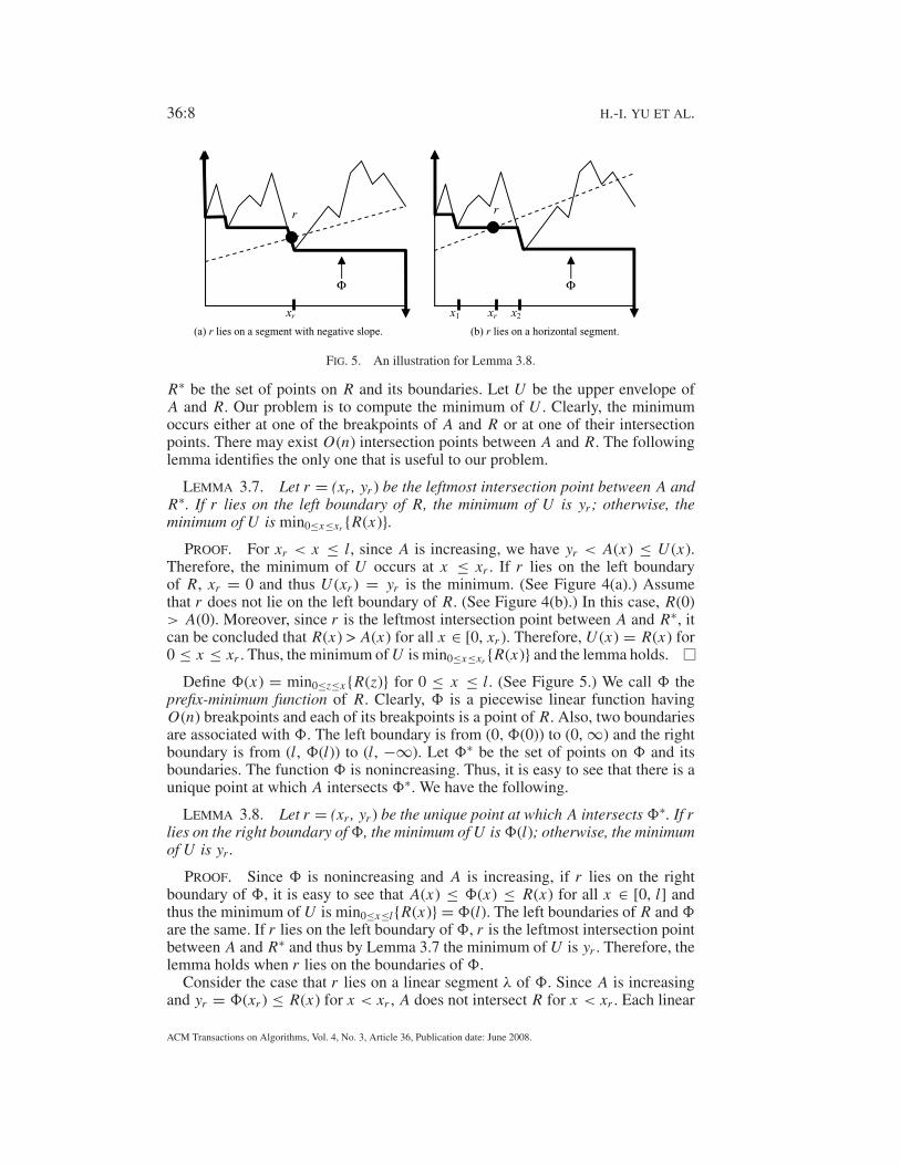
LEMMA 3.7. Let r = (xr , yr ) be the leftmost intersection point between A andR∗. If r lies on the left boundary of R, the minimum of U is yr ; otherwise, theminimum of U is min0≤x≤xr {R(x)}.

PROOF. For xr < x ≤ l, since A is increasing, we have yr < A(x) ≤ U (x).

Therefore, the minimum of U occurs at x ≤ xr . If r lies on the left boundary

of R, xr = 0 and thus U (xr ) = yr is the minimum. (See Figure 4(a).) Assume

that r does not lie on the left boundary of R. (See Figure 4(b).) In this case, R(0)

> A(0). Moreover, since r is the leftmost intersection point between A and R∗, it

can be concluded that R(x) > A(x) for all x ∈ [0, xr ). Therefore, U (x) = R(x) for

0 ≤ x ≤ xr . Thus, the minimum of U is min0≤x≤xr {R(x)} and the lemma holds.

Define �(x) = min0≤z≤x{R(z)} for 0 ≤ x ≤ l. (See Figure 5.) We call � the

prefix-minimum function of R. Clearly, � is a piecewise linear function having

O(n) breakpoints and each of its breakpoints is a point of R. Also, two boundaries

are associated with �. The left boundary is from (0, �(0)) to (0, ∞) and the right

boundary is from (l, �(l)) to (l, −∞). Let �∗ be the set of points on � and its

boundaries. The function � is nonincreasing. Thus, it is easy to see that there is a

unique point at which A intersects �∗. We have the following.

LEMMA 3.8. Let r = (xr , yr ) be the unique point at which A intersects �∗. If rlies on the right boundary of �, the minimum of U is �(l); otherwise, the minimumof U is yr .

PROOF. Since � is nonincreasing and A is increasing, if r lies on the right

boundary of �, it is easy to see that A(x) ≤ �(x) ≤ R(x) for all x ∈ [0, l] and

thus the minimum of U is min0≤x≤l{R(x)} = �(l). The left boundaries of R and �are the same. If r lies on the left boundary of �, r is the leftmost intersection point

between A and R∗ and thus by Lemma 3.7 the minimum of U is yr . Therefore, the

lemma holds when r lies on the boundaries of �.

Consider the case that r lies on a linear segment λ of �. Since A is increasing

and yr = �(xr ) ≤ R(x) for x < xr , A does not intersect R for x < xr . Each linear



segment of � is either horizontal or with negative slope. Assume first that λ is with

negative slope. (See Figure 5(a).) Clearly, in this case, r is a point of R. Since Adoes not intersect R for x < xr , r is the leftmost intersection point between A and

R∗. Therefore, by Lemma 3.7, the minimum of U is min0≤x≤xr {R(x)} = �(xr ) =yr . Next, assume that λ is horizontal. Let (x1, yr ) and (x2, yr ) be the endpoints of λ,

where x1 < x2. Each breakpoint of � is a point of R. Thus, R(x1) = R(x2) = yr .

Since A is increasing, we have A(x1) ≤ R(x1) and A(x2) ≥ R(x2). Thus, for x ∈[x1, x2], there is at least an intersection point between A and R. Let r ′ = (x ′

r , y′r )

be the leftmost such intersection point. Since A does not intersect R for x < xr ,

r ′ is the leftmost intersection point between A and R∗. Therefore, by Lemma 3.7,

the minimum of U is min0≤x≤x ′r{R(x)} = �(x ′

r ). Since x1 ≤ x ′r ≤ x2, we have

�(x ′r ) = yr , which completes the proof of this lemma.

In accordance with Lemma 3.8, after � is computed, our problem becomes to

find the unique point at which A intersects �∗. Since � is nonincreasing and A is

increasing, the finding can be done in O(log n) time by performing binary search

on the linear segments of �. Therefore, we have the following.

LEMMA 3.9. If A is a linear segment with positive slope, using the prefix-minimum function �, the minimum of U can be determined in O(log n) time.

Next, consider the case that A is a linear segment with negative slope. Define the

suffix-minimum function of R as �(x) = minx≤z≤l R(z) for 0 ≤ x ≤ l. Similarly,

we have the following.

LEMMA 3.10. If A is a linear segment with negative slope, using the suffix-minimum function �, the minimum of U can be determined in O(log n) time.

When A consists of two linear segments, the minimum of U is computed as

follows. Since A is a roof function, there is a number x∗ such that A is a linear seg-

ment with positive slope in the interval [0, x∗] and is a linear segment with negative

slope in the interval [x∗, l]. First, we compute m1 = min0≤x≤x∗{max{R(x), A(x)}}.Since A is a linear segment with positive slope in the interval [0, x∗], this can be

done in O(log n) time by changing the right boundary of � into the linear segment

from (x∗, �(x∗)) to (x∗, −∞) and then determining the smallest x ∈ [0, x∗] at

which A intersects �∗. Next, we determine m2 = minx∗≤x≤l{max{R(x), A(x)}}.Similarly, this can be done in O(log n) time by using �. Finally, the minimum of

U is computed as min{m1, m2}.By scanning the breakpoints of R from left to right, � can be computed in O(n)

time. Similarly, � can be computed in O(n) time. We conclude this section with

the following theorem.

THEOREM 3.11. With O(n)-time preprocessing, each query of the radius-adjustment problem can be answered in O(log n) time.

4. The Minmax-Regret 1-Center Problem on Trees

In this section, we assume that the underlying graph G is a tree T = (V , E). For

a tree, the auxiliary graph defined in Section 3.1 is also a tree. Megiddo [1983]

had an O(n)-time algorithm for finding the classical 1-center of a tree. Thus, as

indicated in Averbakh and Berman [1997, 2000a], on a tree the time complexity


36:10 H.-I. YU ET AL.

)b( )a(

(c) (d) (e)

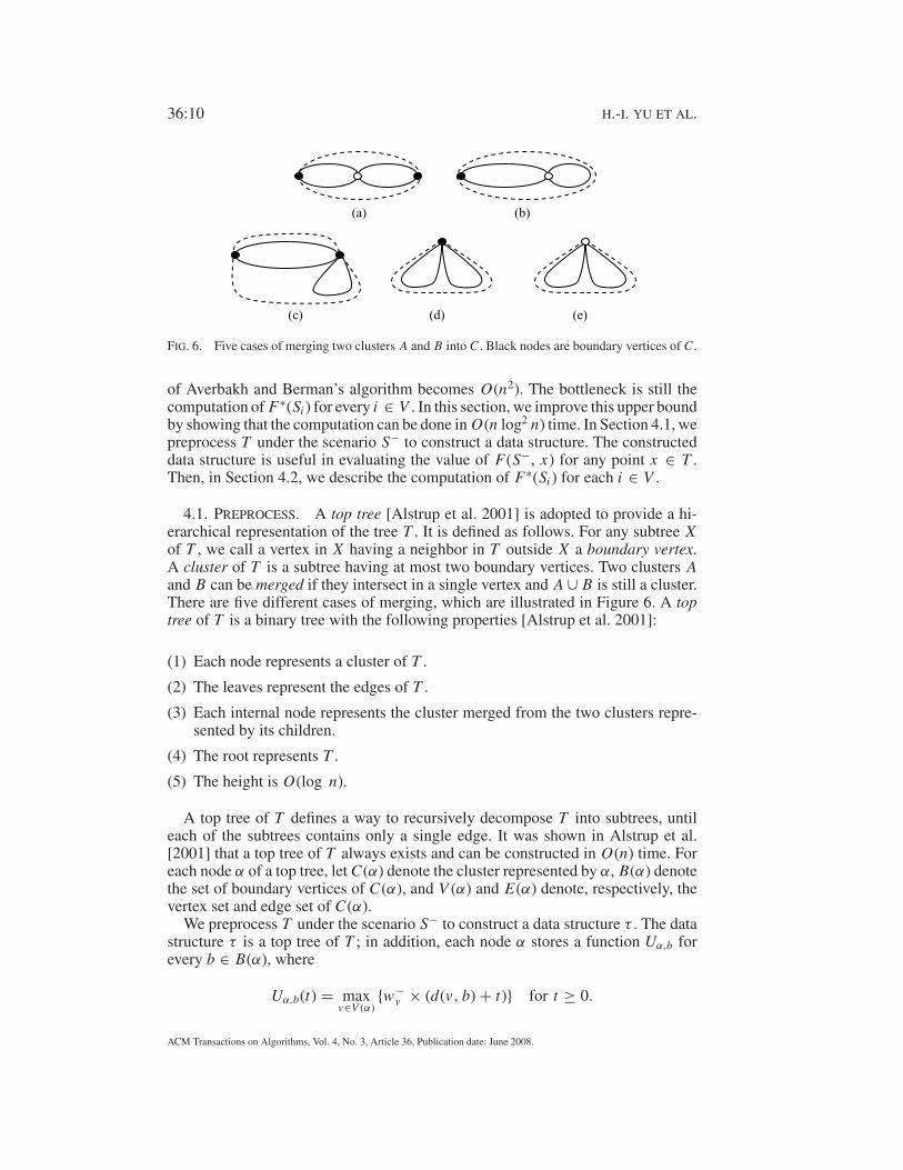
FIG. 6. Five cases of merging two clusters A and B into C . Black nodes are boundary vertices of C .

of Averbakh and Berman’s algorithm becomes O(n2). The bottleneck is still the

computation of F∗(Si ) for every i ∈ V . In this section, we improve this upper bound

by showing that the computation can be done in O(n log2 n) time. In Section 4.1, we

preprocess T under the scenario S− to construct a data structure. The constructed

data structure is useful in evaluating the value of F(S−, x) for any point x ∈ T .

Then, in Section 4.2, we describe the computation of F∗(Si ) for each i ∈ V .

4.1. PREPROCESS. A top tree [Alstrup et al. 2001] is adopted to provide a hi-

erarchical representation of the tree T . It is defined as follows. For any subtree Xof T , we call a vertex in X having a neighbor in T outside X a boundary vertex.

A cluster of T is a subtree having at most two boundary vertices. Two clusters Aand B can be merged if they intersect in a single vertex and A ∪ B is still a cluster.

There are five different cases of merging, which are illustrated in Figure 6. A toptree of T is a binary tree with the following properties [Alstrup et al. 2001]:

(1) Each node represents a cluster of T .

(2) The leaves represent the edges of T .

(3) Each internal node represents the cluster merged from the two clusters repre-

sented by its children.

(4) The root represents T .

(5) The height is O(log n).

A top tree of T defines a way to recursively decompose T into subtrees, until

each of the subtrees contains only a single edge. It was shown in Alstrup et al.

[2001] that a top tree of T always exists and can be constructed in O(n) time. For

each node α of a top tree, let C(α) denote the cluster represented by α, B(α) denote

the set of boundary vertices of C(α), and V (α) and E(α) denote, respectively, the

vertex set and edge set of C(α).

We preprocess T under the scenario S− to construct a data structure τ . The data

structure τ is a top tree of T ; in addition, each node α stores a function Uα,b for

every b ∈ B(α), where

Uα,b(t) = maxv∈V (α)

{w−v × (d(v, b) + t)} for t ≥ 0.



Before presenting the computation of the functions Uα,b, their usage is described

as follows. For any subset K ⊆ V and any point x ∈ T , define

F−(K , x) = maxv∈K

{w−v × d(v, x)},

which is the largest weighted distance from any vertex v ∈ K to x under the scenario

S−. For ease of description, for any node α of τ , we simply write F−(α, x) in place

of F−(V (α), x). Then, we have the following:

LEMMA 4.1. Let α be a node of τ . For any point x ∈ (T \C(α))∪B(α), F−(α,x) = Uα,b(d(b, x)), where b is the boundary vertex nearer to x in B(α).

PROOF. The unique path from x to any vertex in C(α) passes the vertex b.

Therefore, F−(α, x) = maxv∈V (α){w−v ×d(v , x)} = maxv∈V (α){w−

v × (d(v , b)+d(b,

x))} = Uα,b(d(b, x)). Thus, the lemma holds.

For convenience, we call each Uα,b a dominating function of α. Since Uα,b is

the upper envelope of |V (α)| linear functions, by Theorem 3.3, it is a piecewise

linear function having O(|V (α)|) breakpoints. In accordance with Lemma 4.1, with

the dominating functions of a node α of τ , the largest weighted distance from any

vertex in C(α) to any point x outside C(α) can be determined in O(log |V (α)|)time.

We now proceed to discuss the computation of the dominating functions. We do

the computation for each node α of τ , layer by layer from the bottom up. Each leaf

of τ represents an edge of T . Thus, if α is a leaf, the computation of its dominating

functions takes O(1) time. Next, consider the case that α is an internal node. Let bbe a boundary vertex of C(α). Let α1 and α2 be the children of α, and let c be the

intersection vertex of C(α1) and C(α2). Let U1(t) = maxv∈V (α1){w−v × (d(v , b)+ t)}

and U2(t) = maxv∈V (α2){w−v × (d(v , b)+t)}. Since V (α) = V (α1)∪V (α2), Uα,b(t) =

max{U1(t), U2(t)}. Therefore, Uα,b is the upper envelope of U1 and U2. Consider

the function U1. According to the definition of a top tree, B(α) ⊆ B(α1) ∪ B(α2)

and {c} = B(α1) ∩ B(α2). If b ∈ B(α1), U1(t) = Uα1,b(t); otherwise, we have d(v ,

b) = d(v , c) + d(c, b) for each v ∈ C(α1) and thus U1(t) = Uα1,c(d(b, c) + t).Therefore, we obtain U1 from a dominating function of α1 in O(|V (α1)|) time.

Similarly, we obtain U2 from a dominating function of α2 in O(|V (α2)|) time. With

U1 and U2, we then construct Uα,b in O(|V (α1)|+|V (α2)|) = O(|V (α)|) time. Since

α has at most two dominating functions, the computation for α requires O(|V (α)|)time.

The time complexity for computing all the dominating functions is analyzed as

follows. For any node α, the computation time is O(|V (α)|) = O(|E(α)|). No two

clusters of the same layer of τ share a commom edge. Thus, for any layer of τ ,∑α |E(α)| = O(n). Therefore, the computation for all nodes in a layer requires

O(n) time. Since there are O(log n) layers, we have the following:

LEMMA 4.2. The data structure τ can be constructed in O(n log n) time.

4.2. AN IMPROVED ALGORITHM. In this section, by presenting an efficient algo-

rithm to compute F∗(Si ) for every i ∈ V , we show that the minmax-regret 1-center

problem on T can be solved in O(n log2 n) time. We begin with several important

properties of this problem. For any i ∈ V and x ∈ T , define Di (x) = w+i × d(i ,

x). Trivially, Lemma 3.5 can be extended to the following.


36:12 H.-I. YU ET AL.

LEMMA 4.3. For any i ∈ V and x ∈ T , F(Si , x) = max {F(S−, x), Di (x)}.LEMMA 4.4 [MEGIDDO 1983]. For any scenario S ∈ �, the function F(S, ·) is

convex on every simple path in T .

Let c− be the classical 1-center of T under the scenario S−. For each i ∈ V ,

let ci be the classical 1-center of T under the scenario Si . For any two points x ,

y ∈ T , let P(x , y) be the unique path from x to y. The following lemma suggests

a possible range for searching each ci .

LEMMA 4.5. For each i ∈ V , ci is a point on P(c−, i).

PROOF. We prove this lemma by contradiction. Suppose that ci /∈ P(c−, i).

Let x be the point closest to ci on P(c−, i). The point x is on P(c−, ci ). Since

F(S−, ·) is convex on P(c−, ci ) and c− is the classical 1-center under S−, F(S−,

ci ) > F(S−, x) ≥ F(S−, c−). Furthermore, since d(i , ci ) = d(i , x) + d(x , ci ) >

d(i , x), we have Di (ci ) > Di (x). Thus, by Lemma 4.3, F(Si , ci ) = max{F(S−, ci ),

Di (ci )} > max{F(S−, x), Di (x)} = F(Si , x), which contradicts to the definition of

ci . Therefore, the lemma holds.

Let i ∈ V be a vertex and x be a point on P(c−, i). By Lemma 4.4, the value

of F(S−, x) is nondecreasing along the path P(c−, i). On the contrary, the value

of Di (x) is decreasing. Thus, by Lemma 4.3, ci is the point x ∈ P(c−, i) at which

F(S−, ·) and Di intersect. Moreover, F(S−, x) < Di (x) for any x ∈ P(c−, ci )\{ci }and F(S−, x) > Di (x) for any x ∈ P(ci , i)\{ci }. We have the following lemma,

which plays a key role in our algorithm.

LEMMA 4.6. Let i ∈ V be a vertex. For any point x ∈ P(c−, i), ci = x if F(S−,x) = Di (x); otherwise, ci ∈ P(c−, x) if F(S−, x) > Di (x), and ci ∈ P(x, i) ifF(S−, x) < Di (x).

In accordance with Lemma 4.6, if the values F(S−, v) of all v ∈ V are available,

by examining the vertices on P(c−, i) in a binary-search manner, the range for

searching ci can be further restricted to an edge in O(log n) time. We compute

the values F(S−, v) by using the divide-and-conquer strategy. For convenience,

we describe it on the top tree τ . For every node α of τ , layer by layer from the

bottom up, we will compute F−(α, v) for each v ∈ V (α), and we will compute

an array L(α, b) for each b ∈ B(α), where L(α, b) stores the ordering of the

vertices v ∈ V (α) by the distances d(v , b). After the whole computation, we get

F(S−, v) = F−(α0, v) for every v ∈ V , where α0 is the root of τ . If α is a leaf,

since |V (α)| = 2, the computation takes O(1) time. Consider the case that α is

an internal node. Let α1 and α2 be the children of α, and let c be the intersection

vertex of C(α1) and C(α2). We need to compute F−(α, v) for each v ∈ V (α).

Due to the symmetry between C(α1) and C(α2), we only present the computation

for each v ∈ V (α1). Since V (α) = V (α1) ∪ V (α2), F−(α, v) = max{F−(α1, v),

F−(α2, v)} for any v ∈ V . For each v ∈ V (α1), the value F−(α1, v) is available

and, by Lemma 4.1, F−(α2, v) = Uα2,c(d(c, v)). The array L(α1, c) stores the

ordering of the vertices v ∈ V (α1) by the distances d(v , c). By applying a process

similar to merge, we obtain all Uα2,c(d(c, v)) in O(|V (α)|) time from L(α1, c) and

the sequence of breakpoints of Uα2,c. Therefore, the computation of F−(α, v) for

each v ∈ V (α) takes O(|V (α)|) time. Next, consider the computation of L(α, b)

for each b ∈ B(α). By symmetry, we may assume b ∈ B(α1). Clearly, we can



obtain L(α, b) by merging L(α1, b) and L(α2, c) in O(|V (α)|) time. Therefore, the

computation for α takes O(|V (α)|) time in total, from which we conclude that the

whole computation on τ requires O(n log n) time. We have the following lemma.

LEMMA 4.7. F(S−, v) can be computed in O(n log n) time for all v ∈ V .

With the values F(S−, v), in O(n log n) time, we compute the edge ei containing

ci for every i ∈ V as follows. First, we compute c− and then orient T into a rooted

tree with root c−. (In case c− is not a vertex, a dummy vertex is introduced.) Then,

we perform a depth-first traversal on T , during which we maintain the path from

the root c− to the current vertex in an array. And, for each i ∈ V , when i becomes

the current vertex, we perform a binary search to find the edge ei .

Next, we show how to determine the exact position of ci and the value F∗(Si )

for a fixed i ∈ V . If an edge e ∈ T is removed from T , two subtrees are induced.

We denote the vertex set of the subtree containing c− by Y (e) and the vertex set of

the other subtree by Z (e).

LEMMA 4.8. Let e ∈ E be an edge. For any point x ∈ e, F(S−, x) = F−(Y (e),x).

PROOF. Since V = Y (e) ∪ Z (e), F(S−, x) = max{F−(Y (e), x), F−(Z (e), x)}.We prove this lemma by showing that F−(Y (e), x) ≥ F−(Z (e), x) for any x ∈ e.

Let e = (y, z), where y ∈ Y (e) and z ∈ Z (e). Consider moving a point x along the

edge e, from y to z. The distance d(v , x) increases for each v ∈ Y (e) and decreases

for each v ∈ Z (e). Thus, F−(Y (e), x) is increasing and F−(Z (e), x) is decreasing.

Since c− ∈ Y (e), by Lemma 4.4, F(S−, x) is increasing. Therefore, F−(Y (e), x) ≥F−(Z (e), x) for any x ∈ e; otherwise, since F−(Z (e), x) is decreasing, F(S−, x)

would be decreasing at some x .

By Lemmas 4.6 and 4.8, ci is the unique point x∗ ∈ ei at which F−(Y (ei ), ·) and

Di intersect. Moreover, F∗(Si ) = Di (x∗). Therefore, the problem remained is to

determine the unique point x∗ on ei at which F−(Y (ei ), ·) and Di intersect. The

construction of the function F−(Y (ei ), ·) is a costly computation. To avoid it, we

replace it with O(log n) dominating functions. The replacement is based upon the

following lemma.

LEMMA 4.9. For any e ∈ E, there exists a set N of O(log n) nodes in τ suchthat Y (e) = ⋃

α∈N V (α).

PROOF. Let (α0, α1, . . . , αk) be the path in τ from the root to the leaf represent-

ing e. For 1 ≤ j ≤ k, let β j be the sibling node of α j . Let e = (y, z), where y ∈ Y (e)

and z ∈ Z (e). Clearly, any leaf of T is impossible to be c−. Since c− ∈ Y (e), y is

not a leaf. Therefore, y is the intersection vertex of some C(α j ) and C(β j ). Since

V (α0) = V , by repeatedly applying the equation V (α j ) = V (α j+1) ∪ V (β j+1), we

can express V as V (β1) ∪ V (β2) ∪ . . . ∪ V (βk) ∪ V (αk). Since V (αk) = {y, z}and y is the boundary vertex of some C(β j ), V (β1) ∪ V (β2) ∪ . . . ∪ V (βk) ⊇ V \{z} ⊇ Y (e). By the definition of a top tree, e is not contained in each C(β j ). Since

each C(β j ) is a connected subtree, each V (β j ) is either a subset of Y (e) or a subset

of Z (e), from which we conclude that there is a subset N ⊆ {β1, β2, . . . , βk} such

that⋃

α∈N V (α) = Y (e). Since k = O(log n), the lemma holds.

LEMMA 4.10. For any e ∈ E, there exists a set Q of O(log n) dominatingfunctions in τ such that F−(Y (e), x) = maxUα,b∈Q{Uα,b(d(b, x))} for any x ∈ e.


36:14 H.-I. YU ET AL.

PROOF. Let N be a set of O(log n) nodes in τ such that Y (e) = ⋃α∈N V (α).

Consider a node α ∈ N . Since e /∈ E(α), by Lemma 4.1, α has a dominating

function Uα,b such that F−(α, x) = Uα,b(d(b, x)). Since Y (e) = ⋃α∈N V (α), the

lemma holds.

Now, we proceed to show how to determine the unique point x∗ on ei at which

F−(Y (ei ), ·) and Di intersect. According to the proofs of Lemmas 4.9 and 4.10, by

traveling the path in τ from the root to the leaf representing ei , we compute a set Qof dominating functions in τ such that F−(Y (ei ), x) = maxUα,b∈Q{Uα,b(d(b, x))}for any x ∈ ei . Let ei = (y, z), where y ∈ Y (e) and z ∈ Z (e). For ease of discussion,

in the following, ei is regarded as an interval [0, d(y, z)] on the real line, where yand z correspond, respectively, to 0 and d(y, z). For convenience, for any Uα,b ∈ Q,

we say that Di intersects Uα,b at a number x ∈ ei if Di (x) = Uα,b(d(b, x)). We

compute I as the set of numbers x ∈ ei at which Di intersects the functions in

Q. For each Uα,b ∈ Q, since Di is decreasing and Uα,b is increasing, Di and Uα,bhas at most one intersection point, which can be found in O(log n) time by binary

search. Thus, the computation of I takes O(log2 n) time. Then, in O(log n) time,

we compute x∗ as the smallest number in I . The correctness is ensured by the

following lemma.

LEMMA 4.11. Let Q be a set of increasing functions defined on the same intervaland U be the upper envelope of the functions in Q. Let f be a decreasing functionthat intersects U. The smallest number at which f intersects a function in Q is theunique number at which f intersects U.

PROOF. Clearly, U is increasing. Thus, there is a unique number x∗ at which

f intersects U . Since f intersects U at x∗, f (x∗) = U (x∗), and f (x) > U (x) if

x < x∗. Thus, f does not intersect any function in Q at any x < x∗. And thus, x∗is the smallest number at which f intersects a function in Q. Therefore, the lemma

holds.

As mentioned, ci is x∗ and F∗(Si ) = Di (x∗). Therefore, we have the following.

LEMMA 4.12. We can compute ci and F∗(Si ) for all i ∈ V in O(n log2 n) time.

Consequently, we obtain the following theorem.

THEOREM 4.13. The minmax-regret 1-center problem on a tree can be solvedin O(n log2 n) time.

Since all the dominating functions are precomputed and stored in τ , O(n log

n) space is required. The functions are used in (i) the computation of F(S−, v)

for all v ∈ V and (ii) the determination of ci for each i ∈ V . The space can

be reduced to O(n) as follows. We do not compute all the functions in advance.

Consider the computation in (i). It is done layer by layer in a bottom-up fashion on

the top tree τ . At each layer, only dominating functions of the previous layer are

used. Thus, during the computation, we simultaneously compute the dominating

functions layer by layer, keeping only functions of two layers at a time: the current

layer and the previous layer. Next, consider the determination in (ii). To determine

each ci , we need to find the intersection points between Di and a set of O(log

n) dominating functions of different layers. Again, we compute the dominating

functions layer by layer from the bottom up and keep only functions of the current



layer and the previous layer at a time. After the functions of a layer are computed,

before proceeding to the next layer, we find for all Di their intersection points with

these functions.

5. The Minmax-Regret 1-Median Problem on a General Graph

In this section, we consider the minmax-regret 1-median problem on a graph G =(V , E). Averbakh and Berman [2000b] had an O(mn2 log n)-time algorithm for the

problem. In this section, we give a new implementation of their algorithm, which

requires O(mn2 + n3 log n) time. Averbakh and Berman’s algorithm is firstly

described in Section 5.1. Then, our implementation is presented in Section 5.2.

5.1. AVERBAKH AND BERMAN’S ALGORITHM. It is well known that there is

always a vertex that is a solution to the classical 1-median problem [Hakimi 1964].

Thus, for any scenario S ∈ �, miny∈G F(S, y) = miny∈V F(S, y). Therefore, the

regret of x with respect to a scenario S ∈ � can also be expressed as maxy∈V{F(S, x) − F(S, y)}. Consequently, we have

Z (x) = maxS∈�

maxy∈V

{F(S, x) − F(S, y)}= max

y∈VmaxS∈�

{F(S, x) − F(S, y)}.

For any point x ∈ G and vertex y ∈ V , define R(x , y) = maxS∈�{F(S, x) − F(S,

y)}. Then, we have

Z (x) = maxy∈V

R(x, y).

The problem is to find a point x ∈ G that minimizes Z (x). For ease of presentation,

only the computation of the value minx∈G Z (x) is described. For each edge e ∈ E ,

let Z∗e = minx∈e Z (x). Averbakh and Berman solved the minmax-regret 1-median

problem by firstly determining Z∗e for every e ∈ E and then computing minx∈G Z (x)

as the minimum among all Z∗e . Their computation of each Z∗

e takes O(n2 log n) time

and thus their solution to the minmax-regret 1-median problem requires O(mn2 log

n) time. Let e = (a, b) be an edge in G. In the remainder of this subsection, Averbakh

and Berman’s algorithm for computing Z∗e is described. For ease of description, e

is regarded as an interval [a, b] on the real line so that any point on e corresponds

to a real number x ∈ [a, b].

Consider the function R(·, y) for a fixed y ∈ V . For a point x ∈ e, any scenario

S ∈ � that maximizes F(S, x) − F(S, y) is called a worst-case scenario of xaccording to y. For each point x ∈ e and each vertex v ∈ V , let

w x,yv =

{w+

v if d(v, x) > d(v, y), and

w−v if d(v, x) ≤ d(v, y).

For each point x ∈ e, let S(x,y) be the scenario in which the weight of each v ∈ Vis w x,y

v . It is easy to see that S(x,y) is a worst-case scenario of x according to y.

Thus, we have the following lemma.

LEMMA 5.1 [AVERBAKH AND BERMAN 2000b]. R(x, y) = F(S(x,y), x) −F(S(x,y), y).


36:16 H.-I. YU ET AL.

Therefore, R(x , y) = ∑v∈V {w x,y

v × (d(v , x) − d(v , y))}. Since y is fixed, d(v ,

y) is a constant for every v ∈ V . Thus, the slope of R(x , y) at x depends on the

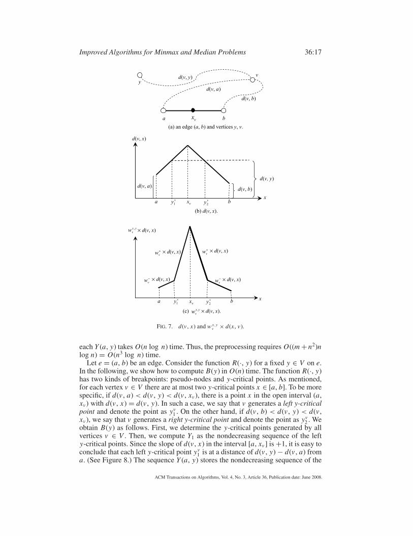
value of w x,yv and the slope of d(v , x). For each v ∈ V , let xv be the point on e that

is farthest from v . (See Figures 7(a) and 7(b).) For convenience, each xv is called a

pseudo-node of e. Consider a fixed v ∈ V . In the interval [a, xv ], d(v , x) is a linear

segment with slope +1. In the interval [xv , b], d(v , x) is a linear segment with slope

−1. Thus, the slope of d(v , x) changes only at the pseudo-node xv . There are at

most two points x ∈ [a, b] with d(v , x) = d(v , y). For ease of presentation, assume

that there are two such points yv1 and yv

2 , where yv1 < yv

2 . (See Figure 7(b).) For

convenience, yv1 and yv

2 are called y-critical points of e. By definition, w x,yv is w−

vfor x ∈ [a, yv

1 ] ∪ [yv2 , b] and is w+

v for x ∈ (yv1 , yv

2 ). Thus, the value of w x,yv changes

only at yv1 and yv

2 . Therefore, in the interval [a, b], w x,yv × d(v , x) is a piecewise

linear function having at most 3 breakpoints. (See Figure 7(c).) Consequently, in

the interval [a, b], R(·, y) is a piecewise linear function having O(n) breakpoints,

including at most n pseudo-nodes and at most 2n y-critical points. The slope of R(·,y) decreases at pseudo-nodes and increases at y-critical points. Let P(e) = (p1, p2,

. . . , pn) be the nondecreasing sequence of all the pseudo-nodes xv , v ∈ V , of e.

Since all breakpoints between two consecutive pseudo-nodes are y-critical points,

R(x , y) is convex in each subinterval [pi , pi+1] of e, 1 ≤ i < n. Note that for any

y ∈ V , e has the same set of pseudo-nodes.

Averbakh and Berman computed the function R(x , y) on e for each y ∈ Vas follows. First, the pseudo-nodes, the y-critical points, and the changes of the

slope at these points are determined, which can be done easily in O(n) time with

the help of the distance matrix. Next, the nondecreasing sequence, denoted by

B(y), of the pseudo-nodes and y-critical points is obtained in O(n log n) time by

sorting. Then, the value and slope of R(x , y) at x = a is determined in O(n) time.

Finally, by scanning the points in B(y), the function R(x , y) on e is computed.

Since the change of the slope at each point in B(y) is known, this final step takes

O(n) time. In total, the computation of each R(x , y) needs O(n log n) time.

Thus, the time complexity for computing all functions R(x , y), y ∈ V , on e is

O(n2 log n).

Next, consider the computation of Z∗e = minx∈e Z (x) = minx∈e {maxy∈V R(x , y)}.

In each subinterval [pi , pi+1] of e, all functions R(x , y), y ∈ V , are convex. Thus,

the minimum of Z (x) within each subinterval [pi , pi+1] can be computed by using

Megiddo’s linear-time algorithm for two-variable linear programming [Megiddo

1983]. Since the number of linear segments of all functions R(x , y), y ∈ V , on eis O(n2), minx∈e Z (x) can be computed in O(n2) time.

5.2. AN IMPROVED ALGORITHM. Averbakh and Berman’s algorithm for com-

puting each Z∗e requires O(n2 log n) time. The bottleneck is the computation of

B(y) for each y ∈ V . In this subsection, we show that with a simple O(n3 log

n)-time preprocessing, each B(y) can be computed in O(n) time.

The preprocessing computes a list for each edge e ∈ E and computes n lists

for each vertex a ∈ V . The list computed for each e ∈ E is P(e), which is the

nondecreasing sequence of all pseudo-nodes of e. The n lists computed for each

a ∈ V are, respectively, denoted by Y (a, y), y ∈ V . Each Y (a, y), y ∈ V , stores

the nondecreasing sequence of the values d(v , y) − d(v , a) of all v ∈ V . By using

sorting and with the help of the distance matrix, the computation of each P(e) and



y

ba

v

d(v, a)

d(v, b)

d(v, y)

xv

(a) an edge (a, b) and vertices y, v.

ba

d(v, a)

d(v, x)

d(v, b)

xv

x

d(v, y)

vy1vy2

(b) d(v, x).

ba

× d(v, x)

xvxvy1

vy2

+vw × d(v, x)+

vw

× d(v, x)−vw × d(v, x)−

vw

× d(v, x)yxvw ,

(c) yxvw , × d(v, x).

FIG. 7. d(v , x) and w x,yv × d(x , v).

each Y (a, y) takes O(n log n) time. Thus, the preprocessing requires O((m + n2)nlog n) = O(n3 log n) time.

Let e = (a, b) be an edge. Consider the function R(·, y) for a fixed y ∈ V on e.

In the following, we show how to compute B(y) in O(n) time. The function R(·, y)

has two kinds of breakpoints: pseudo-nodes and y-critical points. As mentioned,

for each vertex v ∈ V there are at most two y-critical points x ∈ [a, b]. To be more

specific, if d(v , a) < d(v , y) < d(v , xv ), there is a point x in the open interval (a,

xv ) with d(v , x) = d(v , y). In such a case, we say that v generates a left y-criticalpoint and denote the point as yv

1 . On the other hand, if d(v , b) < d(v , y) < d(v ,

xv ), we say that v generates a right y-critical point and denote the point as yv2 . We

obtain B(y) as follows. First, we determine the y-critical points generated by all

vertices v ∈ V . Then, we compute Y1 as the nondecreasing sequence of the left

y-critical points. Since the slope of d(v , x) in the interval [a, xv ] is +1, it is easy to

conclude that each left y-critical point yv1 is at a distance of d(v , y) − d(v , a) from

a. (See Figure 8.) The sequence Y (a, y) stores the nondecreasing sequence of the


36:18 H.-I. YU ET AL.

ba

d(v, a)

d(v, x)

d(v, y)

xv

x

d(v, y)

vy1vy2

d(v, y) – d(v, a) d(v, y) – d(v, b)

d(v, b)

FIG. 8. d(a, yv1 ) and d(b, yv

2 ).

values d(v , y) − d(v , a) of all v ∈ V . Thus, the order of the left y-critical points in

Y1 can be obtained from Y (a, y) in O(n) time by a simple scan. Next, we compute

Y2 as the nondecreasing sequence of the right y-critical points. Since the slope of

d(v , x) in the interval [xv , b] is −1, each right y-critical point yv2 is at a distance of

d(v , y) − d(v , b) from b. The sequence Y (b, y) stores the nondecreasing sequence

of the values d(v , y) − d(v , b) of all v ∈ V . Thus, the order of the right y-critical

points in Y2 can be obtained by scanning the reverse sequence of Y (b, y) in O(n)

time. Finally, B(y) is computed in O(n) time by merging Y1, Y2, and P(e).

With the above computation of B(y), each Z∗e can be computed in O(n2) time.

Thus, we obtain the following.

THEOREM 5.2. The minmax-regret 1-median problem on a general graph canbe solved in O(mn2 + n3 log n) time.

We remark that our algorithm requires O(n3) space to achieve the speedup,

whereas Averbakh and Bermen’s algorithm uses O(n2) space.

6. The Minmax-Regret 1-Median Problem on a Tree

In this section, we consider the minmax-regret 1-median problem on a tree T = (V ,

E). Averbakh and Berman [2003] proposed an O(n log2 n)-time algorithm for the

problem. Their algorithm is firstly described in Section 6.1. Then, in Section 6.2,

an O(n log n)-time improved algorithm is presented.

6.1. AVERBAKH AND BERMAN’S ALGORITHM. An edge that contains a minmax-

regret 1-median is called an optimal edge. Averbakh and Berman’s algorithm con-

sists of two stages. The first stage finds an optimal edge e∗, which requires O(nlog2 n) time. The second stage determines the exact position of a minmax-regret

1-median on the edge e∗, which requires O(n) time. Our improvement is obtained

by giving a more efficient implementation of the first stage. Thus, only the first

stage is described in this subsection.

Let v ∈ V be a vertex. By removing v and its incident edges, T is broken

into several subtrees, each of which is called an open v-branch. For each open

v-branch X, the union of v , X , and the edge connecting v and X is called a v-branch. (See Figure 9.) For any vertex p �= v in T , let B(v , p) be the v-branch

containing p.



v

p

a v-branch B(v, p)

an open v-branch

FIG. 9. Open v-branches and v-branches.

Recall that S− is the scenario in which the weight of every v ∈ V is w−v . Let S+

be the scenario in which the weight of every v ∈ V is w+v . For any subtree X of T ,

let V (X ) be the set of vertices in X . For any vertex a ∈ V and any open a-branch

X , the following auxiliary values are defined:

W +(X ) = ∑v∈V (X ) w+

v , W −(X ) = ∑v∈V (X ) w−

v ,

D+(X, a) = ∑v∈V (X ) w+

v × d(v, a), D−(X, a) = ∑v∈V (X ) w−

v × d(v, a),

F+(a) = ∑v∈V w+

v × d(v, a), F−(a) = ∑v∈V w−

v × d(v, a).

By using dynamic programming, these auxiliary values of all vertices a and all

open a-branches X are precomputed, which takes O(n) time [Averbakh and Berman

2003].

Let R(x , y) and S(x,y) be defined the same as in Section 5.1. Consider the com-

putation of R(x , y) for a pair of vertices x , y ∈ V . An edge is a bisector of a simple

path if it contains the middle point of the path. In case the middle point is located

at a vertex, both the edges connecting the vertex are bisectors. Let (i , j) ∈ E be a

bisector of the path from x to y, where i is closer to x than j . Let X be the open

j-branch containing x and Y be the open i-branch containing y. (See Figure 10.)

By Lemma 5.1, R(x , y) = F(S(x,y), x) − F(S(x,y), y). Since T is a tree, it is easy

to see that under the scenario S(x,y) the weights of all vertices in Y are equal to

their upper bounds w+v and the weights of all vertices in X are equal to their lower

bounds w−v . (See Figure 10.) Thus, F(S(x,y), x) and F(S(x,y), y) can be computed

in O(1) time according to the following equations:

F(S(x,y), x) = F−(x) − D−(Y, i) − d(i, x) × W −(Y ) + D+(Y, i)

+ d(i, x) × W +(Y );

F(S(x,y), y) = F+(y) − D+(X, j) − d( j, y) × W +(X ) + D−(X, j)

+ d( j, y) × W −(X ).

Therefore, given a bisector of x and y, one can compute R(x , y) in O(1) time by

using d(i , x), d( j , y) and the auxiliary values. Based upon the above discussion,

the following lemma is obtained.

LEMMA 6.1 [AVERBAKH AND BERMAN 2003]. Let x ∈ V be a vertex. Giventhe bisectors of the paths from x to all the other vertices, R(x, y) can be computedin O(n) time for all y ∈ V .


36:20 H.-I. YU ET AL.

i j

x y

set to lower

bound −vw

X Y

+vw

set to upper

bound

FIG. 10. The worst-case scenario S(x,y).

For each x ∈ V , let y(x) be a vertex in T such that R(x , y(x)) = maxy∈V R(x ,

y). Since Z (x) = maxy∈V R(x , y) is convex on any simple path in T [Averbakh

and Berman 2000b], the following lemma can be obtained, which shows that for a

given vertex x ∈ V , after y(x) is computed one can reduce the range for searching

an optimal edge e∗ to the x-branch B(x , y(x)).

LEMMA 6.2 [AVERBAKH AND BERMAN 2003]. Let x ∈ V be a vertex. If x =y(x), x is a minmax-regret 1-median of T ; otherwise, B(x, y(x)) contains a minmax-regret 1-median.

A centroid of T is a vertex c ∈ V such that every open c-branch has at most n/2

vertices. It is easy to find a centroid of T in O(n) time [Kariv and Hakimi 1979a,

1979b]. Based upon Lemma 6.2, Averbakh and Berman presented the following

efficient algorithm for finding an optimal edge.

Algorithm 1. OPTIMAL EDGE(T )

Input: a tree T = (V , E)

Output: an optimal edge or a minmax-regret 1-median

begin1 T ← T // ∗ T is the range for searching an optimal edge

2 while (T is not a single edge) do3 begin4 x ← a centroid of T5 for each y ∈ V do compute a bisector of the path from x to y6 for each y ∈ V do R(x , y) ← F(S(x,y), x) − F(S(x,y), y)

7 y(x) ← the vertex that maximizes R(x , y) over all y ∈ V8 if x = y(x) then return (x) //* x is a minmax-regret 1-median

9 else T ← B(x , y(x)) ∩ T //* reduce the search range to a subtree

10 end11 return (T ) //* T is an optimal edge

end

In the course of the above algorithm, T is a subtree of T that is guaranteed to

contain an optimal edge. Since x is the centroid of T , it is easy to conclude that the



size of T is reduced in Line 9 by a factor of at least 4/3. Therefore, the while-loop in

Lines 2–10 performs O(log n) iterations. Consider a fixed iteration. Line 5 can be

done in O(n log n) time as follows. First, T is oriented into a rooted tree with root

x . Then, we perform a depth-first traversal on T . During the traversal, the path from

x to the current vertex is maintained in an array; and, while a vertex y is visited,

a bisector of the path from x to y is computed by performing a binary search. In

Wang et al. [2001], it was shown that given a tree T and a vertex x , it requires (nlog n) time to compute for every vertex y in T a bisector of the path from x to

y. Except Line 5, all computation in the while-loop takes O(n) time. Thus, each

iteration of the while-loop requires O(n log n) time. Therefore, Algorithm 1 finds

an optimal edge in O(n log2 n) time.

6.2. AN IMPROVED ALGORITHM. For each e = (i , j) ∈ E , define Se as the

scenario in which the weight of every vertex v in the open i-branch containing j is

w+v and the weight of every vertex v in the open j-branch containing i is w−

v . Note

that Se is defined on ordered pairs of neighboring vertices and thus S(i, j) �= S( j,i).

A key procedure of the improved algorithm is to compute for every e ∈ E a vertex

that is a classical 1-median under the scenario Se. The computation requires O(nlog n) time and is described firstly in Section 6.2.1. Then, the improved algorithm

is proposed in Section 6.2.2.

6.2.1. Computing Medians. For ease of discussion, throughout this subsection,

we assume that T is rooted at an arbitrary vertex r ∈ V . Let v ∈ V be a vertex.

Denote P(v) as the path from r to v , p(v) as the parent of v , and Tv as the subtree

of T rooted at v . For convenience, the subtrees rooted at the children of v are called

subtrees of v. For any subtree X of T , define the weight of X under a scenario

S ∈ � as W (S, X ) = ∑v∈V (X ) w S

v . For any scenario S ∈ � and v ∈ V , define

δ(S, v) = 2W (S, Tv ) − W (S, T ).

Note that 2W (S, Tv ) − W (S, T ) = W (S, Tv ) − W (S, T \Tv ) and thus δ(S, v) is

equal to the weight difference between Tv and its complement under the scenario

S. By the definition of δ(S, v), it is easy to see the following.

LEMMA 6.3. For any scenario S ∈ �, the function value of δ(S, ·) is decreasingalong any downward path in T .

Under a scenario S ∈ �, a vertex v is a classical 1-median of T if and only if

W (S, X ) ≤ W (S, T )/2 for every open v-branch X [Kariv and Hakimi 1979b]. By

using this property, the following lemma can be obtained.

LEMMA 6.4 [KU ET AL. 2001]. For any scenario S ∈ �, the vertex v ∈ V withthe smallest δ(S, v) > 0 is a classical 1-median.

Under a scenario S ∈ �, T may have more than one median, but it has a unique

vertex v with the smallest δ(S, v) > 0, which is called the median, denoted as m(S).

For any v ∈ V , define the heavy path of v under a scenario S ∈ �, denoted by h(S,

v), as the path starting at v and at each time moving down to the heaviest subtree,

with a tie broken arbitrarily, until a leaf is reached. We have the following.

LEMMA 6.5. Let S ∈ � be a scenario and v ∈ V be a vertex with δ(S, v) > 0.Then, h(S, v) contains the median m(S).


36:22 H.-I. YU ET AL.

FIG. 11. The scenarios Se and Se.

PROOF. We first show that δ(S, x) ≤ 0 for any x ∈ V that is not on h(S, r ). Let

x be a vertex that is not on h(S, r ). Let y be the vertex on h(S, r ) that is closest to

x and z be the child of y that is on the path from y to x . Since z is not on h(S, r ), yhas a child z′ with W (S, Tz′) ≥ W (S, Tz). Therefore, W (S, Tx ) ≤ W (S, Tz) ≤ W (S,

Ty)/2 ≤ W (S, T )/2 and thus δ(S, x) ≤ 0.

Since δ(S, x) ≤ 0 for any x ∈ V that is not on h(S, r ), h(S, r ) contains every

x ∈ V with δ(S, x) > 0. Thus, v is on h(S, r ) and, by Lemmas 6.3 and 6.4, we

conclude that the subpath of h(S, r ) starting from v to the end contains m(S). In

accordance with the construction of a heavy path, the subpath of h(S, r ) starting

from v to the end is just the heavy path h(S, v). Therefore, the lemma holds.

Lemmas 6.3, 6.4, and 6.5 are useful for finding a classical 1-median for a fixed

scenario S ∈ �. In our problem, all scenarios Se, e ∈ E , need to be considered. Let

e = (i , j) be an edge in T such that i is the parent of j . For ease of presentation,

denote Se as the scenario S( j,i). For each v ∈ V , the weight of Tv and the heavy path

of v only depend on the weight assignment to the vertices in Tv . For the scenario

Se, the weight assignment to the vertices in Tj is the same with S+; and the weight

assignment to the vertices in T \Tj is the same with S−. (See Figure 11(a).) On the

other hand, for the scenario Se, the weight assignment to the vertices in Tj is the

same with S−; and the weight assignment to the vertices in T \Tj is the same with

S+. (See Figure 11(b).) Therefore, the following two lemmas can be obtained.

LEMMA 6.6. Let e = (i , j) be an edge in T such that i is the parent of j . Forany v ∈ V ,

W (Se, Tv ) ={

W (S+, Tv ) if v ∈ Tj ,W (S−, Tv ) if v /∈ Tj and v /∈ P(i)

W (S−, Tv ) − W (S−, Tj ) + W (S+, Tj ) if v ∈ P(i); and,

W (Se, Tv ) ={

W (S−, Tv ) if v ∈ Tj ,W (S+, Tv ) if v /∈ Tj and v /∈ P(i),W (S+, Tv ) − W (S+, Tj ) + W (S−, Tj ) if v ∈ P(i).



LEMMA 6.7. Let e = (i , j) be an edge in T such that i is the parent of j . Forany v /∈ P(i),

h(Se, v) ={

h(S+, v) if v ∈ Tj ,h(S−, v) if v /∈ Tj ;

and h(Se, v) ={

h(S−, v) if v ∈ Tj ,h(S+, v) if v /∈ Tj .

In accordance with Lemmas 6.6 and 6.7, maintaining information of T under the

scenarios S+ and S− is very useful to the computation of m(Se) for every e ∈ E .

With a bottom-up computation, we precompute the values W (S+, Tv ) and W (S−,

Tv ) for all v ∈ V in O(n) time. With the precomputed values, for any e ∈ E and

v ∈ V , δ(Se, v) = 2W (Se, Tv ) − W (Se, Tr ) can be determined in O(1) time by

Lemma 6.6. Besides, we preprocess T to construct the heavy path h(S+, v) for

every v ∈ V . The total size of the heavy paths of all v ∈ V is O(n2). However,

they can be constructed in O(n) time as follows. The vertices of T are decomposed

into disjoint paths obtained as described below. At first, we obtain the heavy path

h(S+, r ); then, we decompose each off-path subtree of h(S+, r ) recursively. Clearly,

the decomposition takes O(n) time. Let H1, H2, . . . , and Hk be the disjoint paths

obtained in the above decomposition. Consider a path Hi , 1 ≤ i ≤ k. In accordance

with the definition of a heavy path, the subpath of Hi starting from any vertex v to

the end is the heavy path h(S+, v). Thus, the heavy paths of all vertices on Hi can be

constructed by storing Hi in an array and maintaining for every vertex v two pointers

first+(v) and last+(v), where first+(v) is the position of v in the array and last+(v)

is the position of the last vertex of Hi in the array. Therefore, the construction of

the heavy paths of all the vertices on Hi takes O(|Hi |) time. Consequently, the

construction of the heavy paths of all v ∈ V takes O(n) time. In a similar way, we

also preprocess T to construct the heavy path h(S−, v) for every v ∈ V .

Let H+ = {h(S+, v)|v ∈ V } and H− = {h(S−, v)|v ∈ V }. Let e ∈ E be an

edge. Since the value of δ(Se, ·) decreases along any downward path in T , we can

compute the median m(Se) by firstly finding a path in H+ ∪ H− that contains the

median and then locating the median by performing binary search on the path. The

following two lemmas help in the finding.

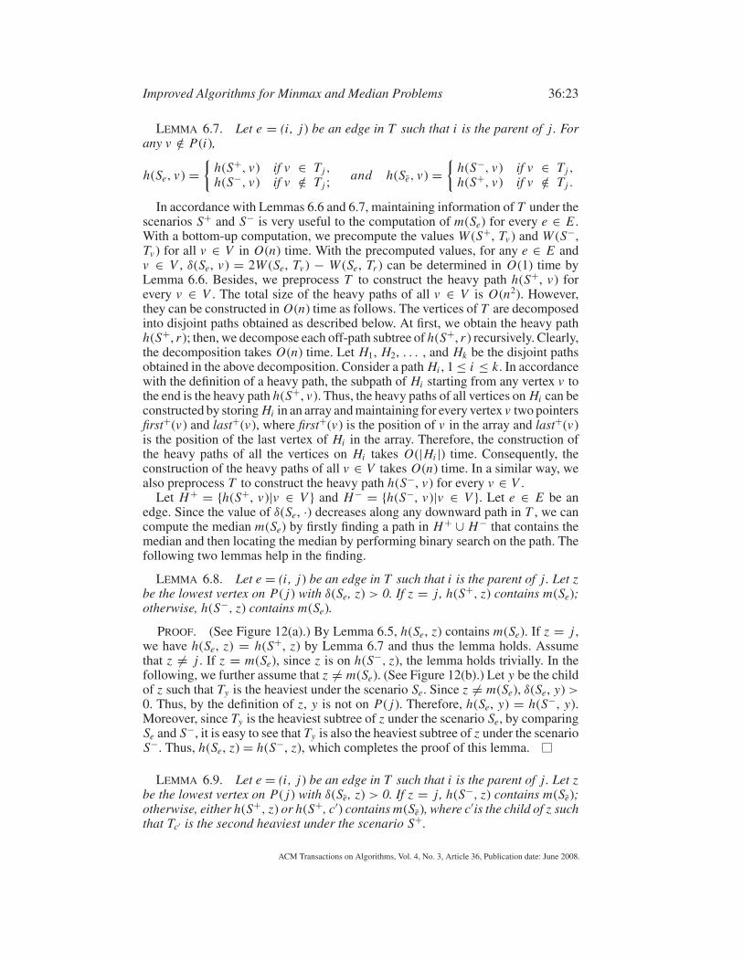
LEMMA 6.8. Let e = (i , j) be an edge in T such that i is the parent of j . Let zbe the lowest vertex on P( j) with δ(Se, z) > 0. If z = j , h(S+, z) contains m(Se);otherwise, h(S−, z) contains m(Se).

PROOF. (See Figure 12(a).) By Lemma 6.5, h(Se, z) contains m(Se). If z = j ,

we have h(Se, z) = h(S+, z) by Lemma 6.7 and thus the lemma holds. Assume

that z �= j . If z = m(Se), since z is on h(S−, z), the lemma holds trivially. In the

following, we further assume that z �= m(Se). (See Figure 12(b).) Let y be the child

of z such that Ty is the heaviest under the scenario Se. Since z �= m(Se), δ(Se, y) >0. Thus, by the definition of z, y is not on P( j). Therefore, h(Se, y) = h(S−, y).

Moreover, since Ty is the heaviest subtree of z under the scenario Se, by comparing

Se and S−, it is easy to see that Ty is also the heaviest subtree of z under the scenario

S−. Thus, h(Se, z) = h(S−, z), which completes the proof of this lemma.

LEMMA 6.9. Let e = (i , j) be an edge in T such that i is the parent of j . Let zbe the lowest vertex on P( j) with δ(Se, z) > 0. If z = j , h(S−, z) contains m(Se);otherwise, either h(S+, z) or h(S+, c′) contains m(Se), where c′is the child of z suchthat Tc′ is the second heaviest under the scenario S+.


36:24 H.-I. YU ET AL.

r

z = j

i

P(i)

h(Se, z)

= h(S+, z)w+

w–

r

j

i

P(i)

h(Se, y)

= h(S–, y)

w+

z

w–

y

(a) z = j. (b) z ≠ j and z ≠ m(Se).

FIG. 12. An illustration for the proof of Lemma 6.8.

PROOF. It is easy to see that the lemma holds for z = j or z = m(Se). Assume

that z �= j and z �= m(Se). Let y be the child of z such that Ty is the heaviest under

the scenario Se. Since z �= m(Se), δ(Se, y) > 0. Thus, y is not on P( j). Let c be

the child of z such that Tc is the heaviest under the scenario S+. Clearly, if j is

not a descendant of c, Tc is also the heaviest subtree of z under the scenario Se.

On the other hand, if j is a descendant of c, either Tc or Tc′ is the heaviest under

the scenario Se. Thus, y is either c or c′. Moreover, since y is not on P( j), h(Se,

y) = h(S+, y). Therefore, either h(S+, c) or h(S+, c′) contains m(Se). Furthermore,

since h(S+, z) ⊃ h(S+, c), we conclude that either h(S+, z) or h(S+, c′) contains

m(Se). Thus, the lemma holds.

Now, we are ready to present our algorithm for computing m(Se) for all e ∈ E .

It is as follows.

Algorithm 2. COMPUTE MEDIANS(T )

Input: a tree T = (V , E)

Output: the classical 1-medians m(Se) of all e ∈ Ebegin

1 Orient T into a rooted tree with an arbitrary root r ∈ V2 Compute W (S+, Tv ), W (S−, Tv ), h(S+, v), and h(S−, v) for all v ∈ V3 for each v ∈ V do4 c′(v) ← the child of v such that Tc′(v) is the second heaviest under S+

5 for each j ∈ V − {r} do (in depth-first search order)

6 begin7 e ← (p( j), j)

8 P( j) ← the path from r to j9 m(Se) ← the classical 1-median under Se

10 m(Se) ← the classical 1-median under Se

11 end12 return ({m(Se)|e ∈ E})

end



The time complexity of Algorithm 2 is analyzed as follows. Lines 1–4 requires

O(n) time. Consider the for-loop in Lines 5–11 for a fixed j ∈ V − {r}. Line 7

takes O(1) time. Since the vertices are processed in depth-first search order, Line 8

also takes O(1) time. Based upon Lemma 6.8, Line 9 is implemented in O(log n)

time as follows. First, we compute z as the lowest vertex on P( j) with δ(Se, z) > 0.

Then, if z = j , we find m(Se) on h(S+, z); otherwise, we find m(Se) on h(S−, z).

The computation of z and the finding of m(Se) are done in O(log n) time by using

binary search. Similarly, based upon Lemma 6.9, Line 10 is implemented in O(log

n) time. Therefore, each iteration of the for-loop takes O(log n) time. There are

n–1 iterations. Thus, the for-loop requires O(n log n) time in total. We obtain the

following.

THEOREM 6.10. The computation of m(Se) of all e ∈ E can be done in O(nlog n) time.

6.2.2. The New Approach. We precompute the medians m(Se) for all e ∈ E .

Also, as in Section 6.1, the auxiliary values W +(X ), W −(X ), D+(X , a), D−(X , a),

F+(a), and F−(a) of all vertices a ∈ V and all open a-branches X are precomputed.

Averbakh and Berman’s algorithm finds an optimal edge by repeatedly reducing

the search range T into a smaller subtree until only one edge is left. Let x be the

centroid of the current search range T . The reduction is done by determining a

vertex y(x) with R(x , y(x)) = maxy∈V R(x , y) and then reducing T into B(x , y(x))

∩ T . A solution to the finding of bisectors is required for their determination of y(x).

The new algorithm is obtained by using a different approach for the determination

of y(x), which is based upon the following lemma.

LEMMA 6.11. For any x ∈ V , there exists an edge e ∈ E such thatR(x, m(Se)) = F(Se, x) − F(Se, m(Se)) = maxy∈V R(x, y).

PROOF. Let y∗ be a vertex such that R(x , y∗) = maxy∈V R(x , y). Let e = (i ,

j) be a bisector of the path from x to y∗, where i is closer to x than j . By Lemma

5.1, R(x , y∗) = F(Se, x) − F(Se, y∗). If y∗ = m(Se), the lemma holds trivially.

In the following, we assume that y∗ �= m(Se). Since m(Se) is a classical 1-median

of T under the scenario Se, F(Se, m(Se)) ≤ F(Se, y∗) and thus F(Se, x) − F(Se,

m(Se)) ≥ F(Se, x) − F(Se, y∗). Then, we have

R(x, m(Se)) = maxS∈�

{F(S, x) − F(S, m(Se))}≥ F(Se, x) − F(Se, m(Se))

≥ F(Se, x) − F(Se, y∗)

≥ R(x, y∗)

≥ maxy∈V

R(x, y).

On the other hand, since m(Se) ∈ V , we have maxy∈V R(x , y) ≥ R(x , m(Se)).

By combining these two statements, we conclude immediately that R(x , m(Se)) =F(Se, x) − F(Se, m(Se)) = maxy∈V R(x , y). Thus, the lemma holds.

In accordance with Lemma 6.11, we modify Algorithm 1 by replacing Lines 5–7

with the following.


36:26 H.-I. YU ET AL.

5. for each e ∈ E do R′(e) ← F(Se, x) − F(Se, m(Se))

6. e ← the edge that maximizes R′(e) over all e ∈ E7. y(x) ← m(Se)

Let e = (i, j) be an edge in T . Let X be the open j-branch containing i and

Y be the open i-branch containing j . Since T is a tree, for every v ∈ V (X ),

we have F(Se, v) = F−(v) − D−(Y , i) − d(i , v) × W −(Y ) + D+(Y , i) + d(i ,

v) × W +(Y ); and for every v ∈ V (Y ), we have F(Se, v) = F+(v) − D+(X , j) −d( j , v) × W +(X ) + D−(X , j) + d( j , v) × W −(X ). By using these two equations,

it is easy to implement the new Line 5 in O(n) time. The new Lines 6 and 7 take

O(n) time. Therefore, Algorithm 1 requires O(n log n) time after the replacement.

THEOREM 6.12. The minmax-regret 1-median problem on a tree can be solvedin O(n log n) time.

7. Concluding Remarks

During the last decade, minmax-regret optimization problems have attracted sig-

nificant research efforts. For many location problems, however, there are still large

gaps between the time complexities of the solutions to their classical versions and

those to their minmax-regret versions. For example, the classical 1-center problem

on a tree can be solved in O(n) time, while the current upper bound for its minmax-

regret version on a tree with uncertainty in both vertex weights and edge lengths is

O(n3 log n) [Burkard and Dollani 2002]. It would be a great challenge to bridge

the gaps.

REFERENCES

ALSTRUP, S., LAURIDSEN, P. W., SOMMERLUND, P., AND THORUP, M. 2001. Finding cores of limited

length. Tech. Rep. The IT University of Copenhagen. (A preliminary version appeared in the 1997

Proceedings of the 5th International Workshop on Algorithms and Data Structures. Lecture Notes in

Computer Science, vol. 1272. Springer-Verlag, New York, 45–54.)

AVERBAKH, I. 2000. Minmax regret solutions for minimax optimization problems with uncertainty. Oper.Res. Lett. 27, 57–65.

AVERBAKH, I. 2003. Complexity of robust single-facility location problems on networks with uncertain

lengths of edges. Disc. Appl. Math. 127, 505–522.

AVERBAKH, I., AND BEREG, S. 2005. Facility location problems with uncertainty on the plane. Disc.Optim. 2, 3–34.

AVERBAKH, I., AND BERMAN, O. 1997. Minimax regret p-center location on a network with demand

uncertainty. Locat. Sci. 5, 247–254.

AVERBAKH, I., AND BERMAN, O. 2000a. Algorithms for the robust 1-center problem on a tree. Europ. J.Oper. Res. 123, 292–302.

AVERBAKH, I., AND BERMAN, O. 2000b. Minmax regret median location on a network under uncertainty.

Inf. J. Comput. 12, 104–110.

AVERBAKH, I., AND BERMAN, O. 2003. An improved algorithm for the minmax regret median problem

on a tree. Networks 41, 97–103.

BRODAL, G., GEORGIADIS, L., AND KATRIEL, I. 2008. An O(n log n) version of the Averbakh-Berman

algorithm for the robust median of a tree. Oper. Res. Lett. 36, 14–18.

BURKARD, R. E., AND DOLLANI, H. 2002. A note on the robust 1-center problem on trees. Ann. Oper.Res. 110, 69–82.

CHEN, B., AND LIN, C.-S. 1988. Minmax-regret robust 1-median location on a tree. Networks 31, 93–103.

DREZNER, Z. 1980. Sensitivity analysis of the optimal location of a facility. Naval Res. Logist. Quart.33, 209–224.

FRANK, H. 1966. Optimum locations on a graph with probabilistic demands. Oper. Res. 14, 409–421.

FRANK, H. 1967. Optimum locations on a graph with correlated normal demands. Oper. Res. 15, 552–557.



GOLDMAN, A. J. 1971. Optimal center location in simple networks. Transport. Sci. 5, 212–221.

HAKIMI, S. L. 1964. Optimal locations of switching centers and the absolute centers and medians of a

graph. Oper. Res. 12, 450–459.

KARIV, O., AND HAKIMI, S. L. 1979a. An algorithmic approach to network location problems. I: The

p-centers. SIAM J. Appl. Math. 37, 513–538.

KARIV, O., AND HAKIMI, S. L. 1979b. An algorithmic approach to network location problems. II: The

p-medians. SIAM J. Appl. Math. 37, 539–560.

KOUVELIS, P., VAIRAKTARAKIS, G., AND YU, G. 1994. Robust 1-median location on a tree in the presence

of demand and transportation cost uncertainty. Working Paper 93/94-3-4. Department of Management

Science and Information Systems, Graduate School of Business, The University of Texas at Austin.

KOUVELIS, P., AND YU, G. 1997. Robust discrete optimization and its applications, Kluwer Academic

Publishers, Dordrecht.

KU, S.-C., LU, C.-J., WANG, B.-F., AND LIN, T.-C. 2001. Efficient algorithms for two generalized 2-

median problems on trees. in Proceedings of the 12th International Symposium on Algorithms andComputation. Lecture Notes on Computer Science, vol. 2223. Springer-Verlag, New York, 768–778.

LABBE, M., THISSE, J.-F., AND WENDELL, R. 1991. Sensitivity analysis in minisum facility location

problems. Oper. Res. 38, 961–969.

MEGIDDO, N. 1983. Linear-time algorithms for linear-programming in R3 and related problems. SIAMJ. Comput. 12, 759–776

MIRCHANDANI, P. B., AND ODONI, A. R. 1979. Location of medians on stochastic networks. Transport.Sci. 13, 85–97.

MIRCHANDANI, P. B., OUDJIT, A., AND WONG, R. T. 1985. Multidimensional extensions and a nested

dual approach for the M-median problem. Europ. J. Oper. Res. 21, 121–137.

NIKULIN, Y. 2004. Robustness in combinatorial optimization and scheduling theory: an annotated bib-

liography. http://www.optimization-online.org/DB HTML/2004/11/995.html.

OUDJIT, A. 1981. Median locations on deterministic and probabilistic multidimensional networks. Ph.D.

dissertation, Rennselaer Polytechnic Institute, Troy.

WANG, B.-F., KU, S.-C., AND SHI, K.-H. 2001. Cost-optimal parallel algorithms for the tree bisector and

related problems. IEEE T. Parall. Distr. 12, 888–898.

WEAVER, J. R., AND CHURCH, R. L. 1983. Computational procedures of location problems on stochastic

networks. Transport. Sci. 17. 168–180.

RECEIVED JUNE 2006; REVISED JULY 2007; ACCEPTED AUGUST 2007


improved algorithms for the minmax-regret 1-center and 1-median problems

Documents