improved algorithms for bipartite network flow

Dartmouth College Dartmouth College

Dartmouth Digital Commons Dartmouth Digital Commons

Open Dartmouth: Peer-reviewed articles by Dartmouth faculty Faculty Work

10-1994

Improved Algorithms for Bipartite Network Flow Improved Algorithms for Bipartite Network Flow

Ravindra K. Ahuja Indian Institute of Technology Kanpur

James B. B. Orlin

Clifford Stein Massachusetts Institute of Technology

Robert E. Tarjan Dartmouth College

Follow this and additional works at: https://digitalcommons.dartmouth.edu/facoa

Part of the Theory and Algorithms Commons

Dartmouth Digital Commons Citation Dartmouth Digital Commons Citation Ahuja, Ravindra K.; Orlin, James B. B.; Stein, Clifford; and Tarjan, Robert E., "Improved Algorithms for Bipartite Network Flow" (1994). Open Dartmouth: Peer-reviewed articles by Dartmouth faculty. 2069. https://digitalcommons.dartmouth.edu/facoa/2069

This Article is brought to you for free and open access by the Faculty Work at Dartmouth Digital Commons. It has been accepted for inclusion in Open Dartmouth: Peer-reviewed articles by Dartmouth faculty by an authorized administrator of Dartmouth Digital Commons. For more information, please contact [email protected].

https://digitalcommons.dartmouth.edu/

https://digitalcommons.dartmouth.edu/facoa

https://digitalcommons.dartmouth.edu/facoa

https://digitalcommons.dartmouth.edu/faculty

https://digitalcommons.dartmouth.edu/facoa?utm_source=digitalcommons.dartmouth.edu%2Ffacoa%2F2069&utm_medium=PDF&utm_campaign=PDFCoverPages

http://network.bepress.com/hgg/discipline/151?utm_source=digitalcommons.dartmouth.edu%2Ffacoa%2F2069&utm_medium=PDF&utm_campaign=PDFCoverPages

https://digitalcommons.dartmouth.edu/facoa/2069?utm_source=digitalcommons.dartmouth.edu%2Ffacoa%2F2069&utm_medium=PDF&utm_campaign=PDFCoverPages

mailto:[email protected]

SIAM J. COMPUT.Vol. 23, No. 5, pp. 906-933, October 1994

1994 Society for Industrial and Applied Mathematics0O2

IMPROVED ALGORITHMS FOR BIPARTITE NETWORK FLOW*

RAVINDRA K. AHUJAt, JAMES B. ORLIN:, CLIFFORD STEIN, AND ROBERT E. TARJAN

Abstract. In this paper, network flow algorithms for bipartite networks are studied. A network G (V, E)is called bipartite if its vertex set V can be partitioned into two subsets VI and V2 such that all edges have oneendpoint in V1 and the other in V2. Let n IVI, nl IVII, n2 1I"21, m IEI and assume without loss ofgenerality that n < n2. A bipartite network is called unbalanced ifn << n2 and balanced otherwise. (This notion is

necessarily imprecise.) It is shown that several maximum flow algorithms can be substantially sped up when appliedto unbalanced networks. The basic idea in these improvements is a two-edge push rule that allows one to "charge"most computation to vertices in Vl, and hence develop algorithms whose running times depend on n rather thann. For example, it is shown that the two-edge push version of Goldberg and Tarjan’s FIFO preflow-push algorithmruns in O(nlm + n3) time and that the analogous version of Ahuja and Odin’s excess scaling algorithm runs inO(nlm + n2 log U) time, where U is the largest edge capacity. These ideas are also extended to dynamic tree

implementations, parametric maximum flows, and minimum-cost flows.

Key words, network flow, bipartite graphs, maximum flow, minimum-cost flow, parametric maximum flow,parallel algorithms

AMS subject classifications. 90B 10,68Q25,68R10

1. Introduction. In this paper, we study network flow algorithms for bipartite networks.A network G (V, E) is called bipartite if its vertex set V can be partitioned into two subsetsV1 and V2 such that all edges have one endpoint in V1 and the other in V2. Let n IV l,n V l, n2 IV21, rn EI, and assume without loss of generality that n < n2. We calla bipartite network unbalanced if n << n2 and balanced otherwise. We show that severalmaximum flow algorithms can be substantially sped up when applied to unbalanced networks.At first glance, it may appear that unbalanced networks are of limited practical utility. This isnot true, however. Gusfield, Martel, and Fernandez-Baca [21 have compiled a list of manypractical applications of unbalanced networks. Further applications of unbalanced networksappear in 14].

Specialized bipartite flow algorithms for unbalanced networks were first studied by Gus-field, Martel, and Fernandez-Baca [21]. They developed modifications of the algorithms ofKarzanov [25] and Malhotra, Pramodh Kumar, and Maheshwari (MPM)[27] for the maximumflow problem that improved their running times from O(n3) to O(nn2). For the boundeddegree case, i.e., when the degree of each vertex in V2 is bounded by a fixed constant, they

*Received by the editors May 20, 1991; accepted for publication (in revised form) June 4, 1993.Department of Industrial and Management Engineering, Indian Institute of Technology, Kanpur 208016, India.

This author’s research was supported in part by Presidential Young Investigator grant 8451517-ECS of the NationalScience Foundation, by grant AFOSR-88-0088 from the Air Force Office of Scientific Research, and by grants fromAnalog Devices, Apple Computers, Inc., and Prime Computer.

Sloan School of Management, Massachusetts Institute of Technology, Cambridge, Massachusetts 02139. Re-search partially supported by Presidential Young Investigator grant 8451517-ECS of the National Science Foundation,by grant AFOSR-88-0088 from the Air Force Office of Scientific Research, and by grants from Analog Devices, AppleComputers, Inc., and Prime Computer.

Department of Computer Science, Dartmouth College, Hanover, New Hampshire 03755. Some of the results inthis paper were part of this author’s undergraduate thesis at Princeton University. Some of the work was done whilethis author was a graduate student at the Laboratory for Computer Science, Massachusetts Institute of Technology,Cambridge, Massachusetts 02139. Research partially supported by a graduate fellowship from AT&T. Additionalsupport provided by Air Force contract AFOSR-86-0078 and by a National Science Foundation PYI grant awardedto David Shmoys, with matching funds from IBM, Sun Microsystems, and the United Parcel Service.

Department of Computer Science, Princeton University, Princeton, New Jersey 08544, and NEC ResearchInstitute, Princeton, New Jersey 08540. Research at Princeton University partially supported by the National ScienceFoundation grant DCR-8605952, and the Office of Naval Research contract N00014-9l-K-1463.

906

Dow

nloa

ded

05/1

4/18

to 1

29.1

70.1

16.2

35. R

edis

trib

utio

n su

bjec

t to

SIA

M li

cens

e or

cop

yrig

ht; s

ee h

ttp://

ww

w.s

iam

.org

/jour

nals

/ojs

a.ph

p

IMPROVED ALGORITHMS FOR BIPARTITE NETWORK FLOW 907

developed a further modification of the MPM algorithm that runs in O(nm + n) time.We suggest several algorithms for the maximum flow problem on unbalanced networks thatimprove the running times of Gusfield et al. for all classes of unbalanced networks.

Gusfield [20] has shown that on a particular bipartite network in which each vertex in V2has constant degree, an algorithm similar to the FIFO preflow-push maximum flow algorithmof Goldberg and Tarjan [15],[16] runs in O(nlm + n) time. Further, he observes that thisresult extends to parametric maximum flow; he solves a series of n maximum flow problemsin O(nlm + n) time. We have similar results, which were obtained independently and applyto a more general class of networks.

We begin with the observation of Gusfield, Martel, and Fernandez-Baca [21 that the timebounds for several maximum flow algorithms automatically improve when the algorithmsare applied without modification to unbalanced networks. A careful analysis of the runningtimes of these algorithms reveals that the worst-case bounds depend on the number of edgesin the longest vertex-simple path in the network. We call this the path length of the networkand denote it by L. For a general network, L may be as large as n 1; but, for a bipartitenetwork, L is at most 2nl + 1. Hence for unbalanced networks the path length is much lessthan n, and we get an automatic improvement in running times. As an example, considerDinic’s algorithm [10] for the maximum flow problem. This algorithm constructs O(L)layered networks and finds a blocking flow in each one. Each blocking flow computationperforms O(m) augmentations and each augmentation takes O(L) time. Consequently, therunning time of Dinic’s algorithm is O(L2m). Thus, when applied to unbalanced networks,the running time of Dinic’s algorithm improves from O(n2m) to O(n]m). Column 3 of Table1.1 summarizes these improvements for several network flow algorithms.

We obtain further running-time improvements by modifying the algorithms. This modifi-cation applies only to preflow-push algorithms [2], [3], [14]-[ 17]; we call it the two-edge pushrule. According to this rule, we always push flow from a vertex in V1 and push flow on twoedges at a time, in a step called a bipush, so that no excess accumulates at vertices in V2. Thisrule allows us to charge all computations to examinations of vertices in V1, though withoutthis rule they might be charged to vertices in V2. As an outcome of this rule, we developalgorithms whose running times depend on n rather than n. We incorporate the two-edgepush rule in several maximum flow algorithms, dynamic tree implementations, a parametricmaximum flow algorithm, and algorithms for the minimum-cost flow problem. Column 4 ofTable 1.1 summarizes the improvements obtained using this approach.

In the presentation to follow, we assume some familiarity with preflow-push algorithmsand we omit many details, since they are straightforward modifications of known results. Thereader interested in further details is urged to consult the appropriate paper or papers discussingthe corresponding result for general networks or the book or the survey paper 18].

2. Preliminaries.

2.1. Network definitions. Let G (V, E) be a directed bipartite network. We associatewith each edge (v, w) in E a finite real-valued capacity u(v, w). Let U max{u(v, w)(v, w) E}. Let source s and sink be the two distinguished vertices in the network. Wemake the assumption that s 6 V2 and 6 V. We further assume, without loss of generality,that if (v, w) is in E then so is (w, v), and that the network contains no parallel edges. Wedefine the edge incidence list I(v) of a vertex v 6 V to be the set of edges directed out ofvertex v, i.e., I(v) {(v, w) (v, w) E}.

2.2. Flow. Aflow is a function f E -- R satisfying

(2.1) f(v, w) <_ u(v, w) (v, w) E,

Dow

nloa

ded

05/1

4/18

to 1

29.1

70.1

16.2

35. R

edis

trib

utio

n su

bjec

t to

SIA

M li

cens

e or

cop

yrig

ht; s

ee h

ttp://

ww

w.s

iam

.org

/jour

nals

/ojs

a.ph

p

908 R.K. AHUJA, J. B. ORLIN, C. STEIN, AND R. E. TARJAN

TABLE 1.1A summary of the results discussed in this paper. Column 2 contains previously known results for general

graphs. Column 3 gives bounds on bipartite networks based on the improved bound on L. Column 4 gives our newresults based on the two-edge push rule.

Algorithm

Maximum Flows

Dinic 10]

Karzanov [25]

MPM [27]

FIFO preflow-push

[15], [16]

Highest label

preflow-push [7]

Excess scaling [2]

Wave scaling [3]

FIFO w/dynamic trees

[15],[16]

Parallel excess scaling [2]

Parametric Flows

GGT [14]

GGT w/

dynamic trees 14]

Min-Cost Flows

Cost scaling 17]

Cost scaling w/

dynamic trees 17]

Running time,general network

n2mn

n

n

nm+ n log U

nm + nZ/U

nm log(-

n log U log(- ),

[m/n processors

n

nm log(-k-

n log(nC)

nm log()log(nC)

Running time,bipartite network

n21 mnn[21]nn[21]n21 n

nlm + nln log U

ntm +nnvU

nlm log(-)

n n log U log(-ff ),

[m/n processors

nln

nlm log()

n21n log(n C)

nlm log(-)log(n C)

Running time,modified version

does not apply

nm + n2does not apply

nlm + nnlm

+ min{n, n/-}n m + n2 log U

nlm + n2 IUnm log( + 2)

n log U log(),[m/n processors

nlm log( + 2)

n m + n31 log(n C)

nlm log("-+2)log(n C)

(2.2) f(v, w) -f(w, v) V(v, w)_E,

(2.3) Ef(v’w)=O Yw 6 V-{s,t}.vEV

The value of a flow is the net flow into the sink, i.e.,

Ifl f(v, t).vEV

The maximumflow problem is to determine a flow f for which Ifl is maximum.

2.3. Preflow. A preflow is a function f E --+ R that satisfies conditions (2.1), (2.2),and the following relaxation of condition (2.3)"

Ef(v’w) >0 Yw_ V-{s}.(2.4)vV

Dow

nloa

ded

05/1

4/18

to 1

29.1

70.1

16.2

35. R

edis

trib

utio

n su

bjec

t to

SIA

M li

cens

e or

cop

yrig

ht; s

ee h

ttp://

ww

w.s

iam

.org

/jour

nals

/ojs

a.ph

p


The maximum flow algorithms described in this paper maintain a preflow during thecomputation. For a given preflow f, we define, for each vertex w V, the excess e(w)vz f(v, w). A vertex other than with strictly positive excess is called active.

2.4. Residual capacity. With respect to a preflow f, we define the residual capacityuf(v, w) of an edge (v, w) to be uf(v, w) u(v, w) f(v, w). The residual network is thenetwork consisting only of edges that have positive residual capacity.

2.5. Distance labels. A distance function d V -- Z+U{cx} with respect to the residualcapacities uf(v, w) is a function mapping the vertices to the nonnegative integers. We saythat a distance function is valid if d(s) 2nl, d(t) 0, and d(v) < d(w) + for every edge(v, w) in the residual network. We call a residual edge with d(v) d(w) + eligible. Theeligible edges are exactly the edges on which we push flow.

We refer to d(v) as the distance label of vertex v. It can be shown that if the distancelabels are valid, then each d(v) is a lower bound on the length of the shortest path from v toin the residual network. If there is no directed path from v to t, however, then d(v) is a lowerbound on 2n plus the length of the shortest path from v to s. If, for each vertex v, the distancelabel d(v) equals the minimum of the length of the shortest path from v to and 2nl plus thelength of the shortest path from v to s, then we call the distance labels exact.

3. The generic preflow-push algorithm on bipartite networks. All maximum flowalgorithms described in this paper are preflow-push algorithms, i.e., algorithms that maintaina preflow at every stage. They work by examining active vertices and pushing excess fromthese vertices to vertices estimated to be closer to t. If is not reachable, however, an attemptis made to push the excess back to s. Eventually, there will be no excess on any vertex otherthan t. At this point the preflow is a flow, and moreover it is a maximum flow 15], 16]. Thealgorithms use distance labels to measure the closeness of a vertex to the sink or the source.

The generic preflow-push algorithm consists ofa preprocessing stage followed by repeatedapplication of a procedure called push/relabel. These two procedures appear in Fig. 3.1.

procedure preprocessbegin

f=O;push u(s, v) units of flow on each edge (s, v) 6 I(s);compute the exact distance label function d by

backward breadth-first searches from and from sin the residual network;

endprocedure push/relabel(v)begin

if there is an eligible edge (v, w)then

begin select an eligible edge (v, w);push d min{e(v), uf(v, w)} units of flow from v to w

endelse replace d(v) by min{d(w) + (v, w) I(v) and uf(v, w) > O}

end

FIG. 3.1. Two proceduresfor the generic preflow-push algorithm.

Increasing the flow on an edge is called a push through the edge. We say a push of 3units of flow on edge (v, w) is saturating if 6 uf(v, w) and nonsaturating otherwise. Anonsaturating push at vertex v reduces e(v) to zero. We refer to the process of increasing thedistance label of a vertex as a relabel operation. The purpose of the relabel operation is tocreate at least one eligible edge on which the algorithm can perform further pushes.

Dow

nloa

ded

05/1

4/18

to 1

29.1

70.1

16.2

35. R

edis

trib

utio

n su

bjec

t to

SIA

M li

cens

e or

cop

yrig

ht; s

ee h

ttp://

ww

w.s

iam

.org

/jour

nals

/ojs

a.ph

p


Not specified in Fig. 3.1 is an efficient way to choose edges for pushing steps. We assumethe same mechanism as that proposed by Goldberg and Tarjan [15], [16]. The algorithmmaintains the incidence list I(v) for each vertex v, and a pointer into each such list indicatinga current edge. Initially the current edge of each incidence list is the first edge on the list. Toperform push/relabel(v), the current edge pointer for v is moved through the list I (v) until itindicates an eligible edge or it reaches the end of the list. In the former case, a push is doneon the current edge. In the latter case, a relabel of v is done and the pointer is reset to indicatethe first edge on I(v). Figure 3.2 contains the algorithm preflow-push, which combines thetwo subroutines of Fig. 3.1. At the termination of the algorithm, each vertex in V {s, t} haszero excess; thus the final preflow is a flow. It is easy to establish that this flow is maximum.We shall briefly discuss the worst-case time complexity of the algorithm. (We refer the readerto the paper of Goldberg and Tarjan 16] for a complete discussion of the algorithm.)

algorithm preflow-pushbegin

preprocess;while the network contains an active vertex dobegin

select an active vertex v;push/relabel(v

endend

FIG. 3.2. Algorithm preflow-push.

We begin by stating two lemmas from 15] and [16].LEMMA 3.1 [15], [16]. The generic preflow-push algorithm maintains valid distance

labels at each step. Moreover, each relabeling ofa vertex v strictly increases d(v).LEMMA 3.2 15], 16]. At any time during the preflow-push algorithm, for each vertex v

with positive excess, there is a directed pathfrom vertex v to vertex s in the residual network.Now we can derive the necessary results specific to bipartite networks.COROLLARY 3.3. For each active vertex v, d(v) < 4n.Proof. When a vertex v is relabeled, it has positive excess, and hence the residual network

contains a path P from v to s. Since the vertices on this path are alternately in V and V2, themaximum possible length of the path is 2n. Since d(s) 2n and, for every edge (w, x) onP, d(w) < d(x) + 1, it must be the case that d(v) < d(s) + 2n 4n. U

COROLLARY 3.4. The number of relabel steps is O(nn). Further, the time spent per-forming relabels is O(nm). The time spent scanning edges while finding eligible edges onwhich to pushflow is also 0(n m).

Proof. The first statement follows directly from Lemma 3.1 and Corollary 3.3. The secondstatement follows from the fact that in order to relabel a vertex v, we must look at all ofthe edgesin I(v). Hence, wecan bound the total relabeling time by O((vv II(v)l)(4n)) O(nm).The same bound holds for the time spent finding edges on which to push flow. [3

COROLLARY 3.5. The preflow-push algorithm performs O(nm) saturating pushes.

Proof. Between two consecutive saturating pushes on an edge (v, w), both d(v) and d(w)must increase by 2. By Lemma 3.1 and Corollary 3.3, only O(n 1) saturating pushes can bedone on (v, w). Summing over all edges gives the bound.

LEMMA 3.6. The preflow-push algorithm performs 0 (n2m nonsaturating pushes.

Proof Omitted. (Analogous to the proof of Lemma 3.10 in 16].) [3

Dow

nloa

ded

05/1

4/18

to 1

29.1

70.1

16.2

35. R

edis

trib

utio

n su

bjec

t to

SIA

M li

cens

e or

cop

yrig

ht; s

ee h

ttp://

ww

w.s

iam

.org

/jour

nals

/ojs

a.ph

p


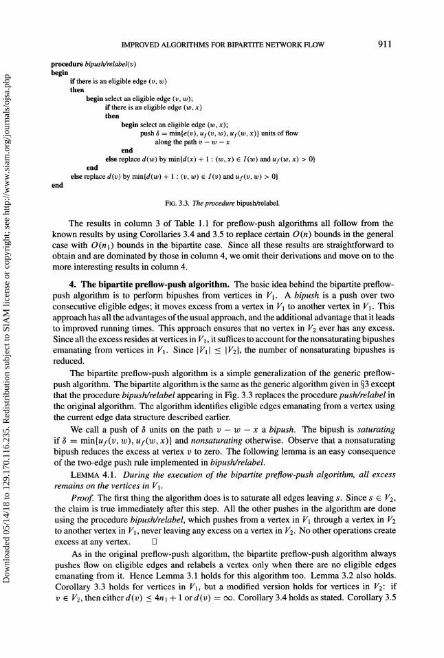
procedure bipush/relabel(vbegin

if there is an eligible edge (v, w)then

begin select an eligible edge (v, w);if there is an eligible edge (w, x)then

begin select an eligible edge (w, x);push d min{e(v), uf(v, w), uf(w, x)} units of flow

along the path v to xend

else replace d(w) by min{d(x) + (w,x) I(w) and uf(w,x) > 0}end

else replace d(v) by min{d(w) + (v, w) I(v) and uf(v, w) > 0}end

FIG. 3.3. The procedure bipush/relabel.

The results in column 3 of Table 1.1 for preflow-push algorithms all follow from theknown results by using Corollaries 3.4 and 3.5 to replace certain O(n) bounds in the generalcase with O(n) bounds in the bipartite case. Since all these results are straightforward toobtain and are dominated by those in column 4, we omit their derivations and move on to themore interesting results in column 4.

4. The bipartite preflow-push algorithm. The basic idea behind the bipartite preflow-push algorithm is to perform bipushes from vertices in V. A bipush is a push over twoconsecutive eligible edges; it moves excess from a vertex in V to another vertex in V. Thisapproach has all the advantages ofthe usual approach, and the additional advantage that it leadsto improved running times. This approach ensures that no vertex in V2 ever has any excess.Since all the excess resides at vertices in V, it suffices to account for the nonsaturating bipushesemanating from vertices in V. Since Vl _< V2l, the number of nonsaturating bipushes isreduced.

The bipartite preflow-push algorithm is a simple generalization of the generic preflow-push algorithm. The bipartite algorithm is the same as the generic algorithm given in 3 exceptthat the procedure bipush/relabel appearing in Fig. 3.3 replaces the procedure push/relabel inthe original algorithm. The algorithm identifies eligible edges emanating from a vertex usingthe current edge data structure described earlier.

We call a push of units on the path v w x a bipush. The bipush is saturatingif/ min{uf(v, w), uf(w, x)} and nonsaturating otherwise. Observe that a nonsaturatingbipush reduces the excess at vertex v to zero. The following lemma is an easy consequenceof the two-edge push rule implemented in bipush/relabel.

LEMMA 4.1. During the execution of the bipartite preflow-push algorithm, all excessremains on the vertices in V.

Proof. The first thing the algorithm does is to saturate all edges leaving s. Since s 6 V2,the claim is true immediately after this step. All the other pushes in the algorithm are doneusing the procedure bipush/relabel, which pushes from a vertex in V through a vertex in V2to another vertex in V, never leaving any excess on a vertex in V2. No other operations createexcess at any vertex. [3

As in the original preflow-push algorithm, the bipartite preflow-push algorithm alwayspushes flow on eligible edges and relabels a vertex only when there are no eligible edgesemanating from it. Hence Lemma 3.1 holds for this algorithm too. Lemma 3.2 also holds.Corollary 3.3 holds for vertices in V, but a modified version holds for vertices in V2: ifv V2, then either d(v) < 4nl + or d(v) cx. Corollary 3.4 holds as stated. Corollary 3.5

Dow

nloa

ded

05/1

4/18

to 1

29.1

70.1

16.2

35. R

edis

trib

utio

n su

bjec

t to

SIA

M li

cens

e or

cop

yrig

ht; s

ee h

ttp://

ww

w.s

iam

.org

/jour

nals

/ojs

a.ph

p


translates into a bound of O(nlm) saturating bipushes. The Lemma 3.6 bound of O(nm) onnonsaturating pushes becomes a bound of O(nm) on nonsaturating bipushes. Thus we getthe following result.

THEOREM 4.2. The bipartite preflow-push algorithm runs in O(n2m time.

We now define the concept of a vertex examination. In an iteration, the generic bipar-tite preflow-push algorithm selects an active vertex v and performs a saturating bipush or anonsaturating bipush or relabels a vertex. In order to develop more efficient algorithms, weincorporate the rule that whenever the algorithm selects an active vertex v V1, it keepspushing flow from that vertex until either its excess becomes zero or it is relabeled. Conse-quently, there may be several saturating bipushes followed either by a nonsaturating bipushor a relabel operation; there will in general also be relabelings of vertices in V2. We associatethis sequence of operations with a vertex examination. We shall henceforth assume that thebipartite preflow-push algorithm follows this rule.

5. Specific implementations ofthe bipartite preflow-push algorithm. The bottleneckin the bipartite preflow-push algorithm is the time spent doing nonsaturating bipushes. Thereare two orthogonal approaches to reducing this time. One approach is to reduce the numberof nonsaturating bipushes by selecting the vertices for bipush/relabel operations cleverly. Weshall consider several such selection rules in 5.1-5.4. The second approach is to reduce thetime spent per nonsaturating bipush. The idea is to use a sophisticated data structure in order topush flow along a whole path in one step, rather than pushing flow along a single pair of edges.We shall study this approach in 5.5. Finally, in 5.6 we study a parallel implementation ofone version of the bipartite preflow-push algorithm.

5.1. The first-in first-out (FIFO) algorithm. The FIFO preflow-push algorithm exam-ines active vertices in first-in, first-out (FIFO) order. The algorithm maintains a queue Q ofactive vertices. It selects a vertex v from the front of Q and performs pushes from v whileadding newly active vertices to the rear of Q. The algorithm examines v until either it be-comes inactive or it is relabeled. In the latter case, v is added to the rear of Q. The algorithmterminates when Q is empty. Goldberg and Tarjan 17] showed that the FIFO algorithm per-forms O(n3) nonsaturating pushes. We show, using a similar analysis, that the number ofnonsaturating bipushes in the bipartite case is O(n).

For the purpose of the analysis, we partition the sequence of vertex examinations intoseveral passes. The first pass consists of examining the vertices that become active during thepreprocess step. For k >_ 2, the kth pass consists of examining all vertices that were added tothe queue during the k st pass.

LEMMA 5.1. The number ofpasses over Q is O(n).Proof Let max{d(v)lv is active}. The initial value of is at most 4n. Consider

the effect that a pass over Q can have on . If, during the pass, no vertex in V is relabeled,then the excess at every vertex is pushed to a vertex with a distance label smaller by at leasttwo, and consequently decreases by at least two. If some vertex in V is relabeled duringthe pass, however, then can increase or remain the same. In such a case the increase inis bounded by the largest increase in any distance label. Hence, by Corollary 3.3, the totalincrease in over all passes is at most 4n2. Consequently, the total number of passes is

o(,).Now observe that any pass examines each vertex in V at most once and each vertex

examination performs at mostone nonsaturating bipush. Consequently, the algorithm performsO(n) nonsaturating bipushes. We noted in the previous section that all other operations take0(n m) time. Thus we obtain the following result.

Dow

nloa

ded

05/1

4/18

to 1

29.1

70.1

16.2

35. R

edis

trib

utio

n su

bjec

t to

SIA

M li

cens

e or

cop

yrig

ht; s

ee h

ttp://

ww

w.s

iam

.org

/jour

nals

/ojs

a.ph

p


THEOREM 5.2. The bipartite FIFO preflow-push algorithm runs in O(nlm -!- n) time.

We note that this bound is also achieved by Karzanov’s algorithm [25] if it is implementedusing the two-edge push rule. A modification of Karzanov’s algorithm by Tarjan [36], whichhe calls the wave algorithm, also has the same time bound. The analysis of both of thesealgorithms is straightforward and hence omitted.

5.2. The highest-label preflow-push algorithm. The highest-label preflow-push algo-rithm always pushes from an active vertex with highest distance label. This rule can beimplemented using a simple bucketing approach so that the overhead for vertex selection is

O(n). The nonsaturating bipushes performed by the algorithm can be divided into passes.A pass consists of all bipushes that occur between two consecutive relabel steps of verticesin//’1. Within a pass, vertices in//’2 can possibly be relabeled several times. Notice that inthis algorithm, excesses that are most distant from the sink are pushed down two levels at atime. Consequently, if the algorithm does not relabel any vertex during n consecutive vertexexaminations, all excess reaches the sink and the algorithm terminates. Since the algorithmperforms O(n) relabel operations on vertices in 1/’1, we immediately obtain a bound of O(n)on the number of vertex examinations. As each vertex examination entails at most one non-saturating bipush, this gives a bound of O(n3) on the number of nonsaturating bipushes anda bound of O(nlm + n3) on the running time of the algorithm.

Cheriyan and Maheshwari [7] showed by a clever argument that the highest label preflow-push algorithm performs O(n2dr-) nonsaturating pushes for general networks. Modifyingtheir argument to fit the bipartite case, we obtain a running time of O(nlm + min{n, n}).This improves the above bound of O(nlm + n) if < nl. We shall give a potential-basedargument that is slightly different from the analysis of Cheriyan and Maheshwari.

We focus on the set of edges that are both current and eligible; we call these edges live.Recall that an edge (v, w) is eligible if it has positive residual capacity and d(v) d(w) + 1;(v, w) is current if the current edge pointer for vertex v indicates (v, w). Each vertex has atmost one outgoing live edge, and the live edges form no cycles since d(v) > d(w) if (v, w) isa live edge. Thus the set of live edges defines a forest, which we call the live forest. We callan active vertex maximal if it has no active proper descendant in the live forest. For a vertexv, let desc(v) be the number of descendants of v in the live forest, including v itself, that arein V1. Let p be a positive integer parameter whose value we shall choose later. For a maximalactive vertex v, we define the uncounted cost c(v) of v to be min{0, desc(v) p}. For anyvertex v that is not maximal active, we define c(v) 0. We use the sum ’’vz c(v) to helpbound the number of nonsaturating bipushes.

We wish to count nonsaturating bipushes. Our strategy is to charge nonsaturating bi-pushes against changes in current edges, relabelings, increases in the total uncounted cost,and certain other events. We shall obtain an overall bound of O(nlmp + n3/p) on the num-ber of nonsaturating bipushes. Choosing p max{l, [n/dr- ]} then gives a bound ofO(min{nlm + n, n/-}) on the number of nonsaturating bipushes.

Define a pass of the algorithm to be a maximal interval of time during which all verticesselected for bipush/relabel steps have the same distance label. A pass terminates either whena relabeling occurs or when all excess at vertices with maximum distance label is moved tovertices of distance label lower by two.

LEMMA 5.3. The total number ofnonsaturating bipushes is O(nmp + n/p).Proof. An argument like that in Lemma 5.1 shows that the total number of passes is

O(n). Consider the nonsaturating bipushes that occur during a pass. Every vertex fromwhich a bipush occurs is maximal active. For a vertex v, call a nonsaturating bipush from vlarge if c(v) 0 before the bipush and small otherwise. Two vertices v and w from which

Dow

nloa

ded

05/1

4/18

to 1

29.1

70.1

16.2

35. R

edis

trib

utio

n su

bjec

t to

SIA

M li

cens

e or

cop

yrig

ht; s

ee h

ttp://

ww

w.s

iam

.org

/jour

nals

/ojs

a.ph

p


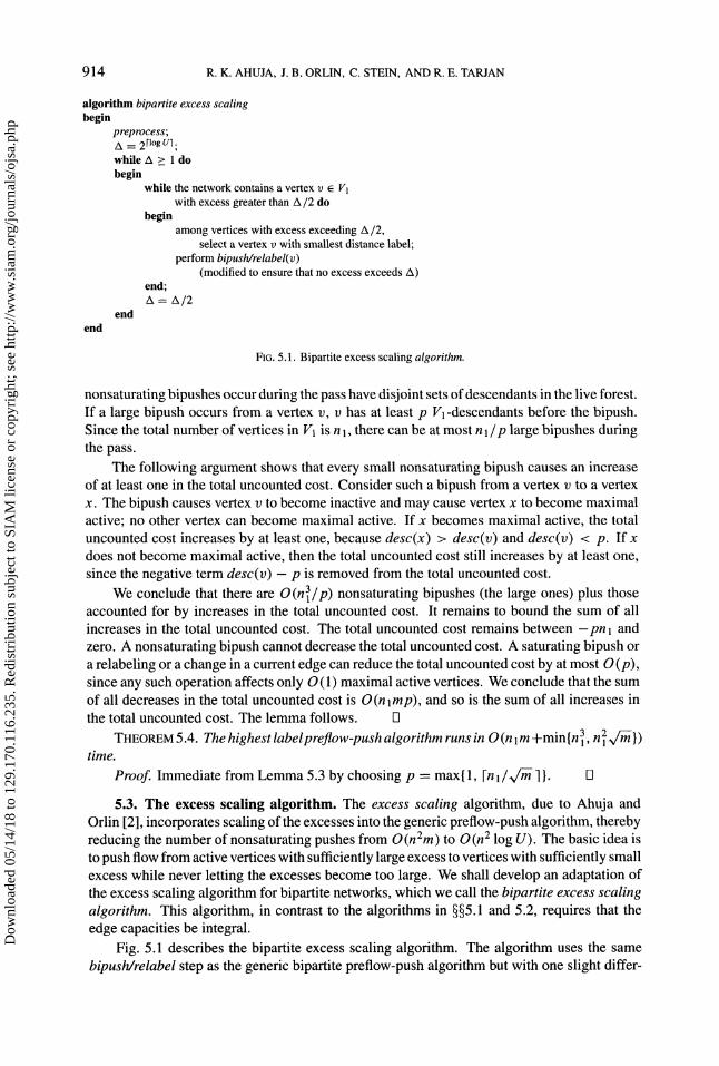
algorithm bipartite excess scalingbegin

preprocess;A 2rlg u];while A > dobegin

while the network contains a vertex v Vlwith excess greater than A/2 do

beginamong vertices with excess exceeding A/2,

select a vertex v with smallest distance label;perform bipush/relabel(v)

(modified to ensure that no excess exceeds A)end;

endend

FIG. 5.1. Bipartite excess scaling algorithm.

nonsaturating bipushes occur during the pass have disjoint sets of descendants in the live forest.If a large bipush occurs from a vertex v, v has at least p V-descendants before the bipush.Since the total number of vertices in V is n 1, there can be at most n 1/P large bipushes duringthe pass.

The following argument shows that every small nonsaturating bipush causes an increaseof at least one in the total uncounted cost. Consider such a bipush from a vertex v to a vertexx. The bipush causes vertex v to become inactive and may cause vertex x to become maximalactive; no other vertex can become maximal active. If x becomes maximal active, the totaluncounted cost increases by at least one, because desc(x) > desc(v) and desc(v) < p. If xdoes not become maximal active, then the total uncounted cost still increases by at least one,since the negative term desc(v) p is removed from the total uncounted cost.

We conclude that there are O(n/p) nonsaturating bipushes (the large ones) plus thoseaccounted for by increases in the total uncounted cost. It remains to bound the sum of allincreases in the total uncounted cost. The total uncounted cost remains between -pnl andzero. A nonsaturating bipush cannot decrease the total uncounted cost. A saturating bipush ora relabeling or a change in a current edge can reduce the total uncounted cost by at most O(p),since any such operation affects only O (1) maximal active vertices. We conclude that the sumof all decreases in the total uncounted cost is O(nmp), and so is the sum of all increases inthe total uncounted cost. The lemma follows. [3

THEOREM 5.4. The highest labelpreflow-push algorithm runs in 0 (n m+min{n, n24})time.

Proof. Immediate from Lemma 5.3 by choosing p max{ 1, [n/v/-- }. [3

5.3. The excess scaling algorithm. The excess scaling algorithm, due to Ahuja andOrlin [2], incorporates scaling ofthe excesses into the generic preflow-push algorithm, therebyreducing the number of nonsaturating pushes from O(nZm) to O (n2 log U). The basic idea isto push flow from active vertices with sufficiently large excess to vertices with sufficiently smallexcess while never letting the excesses become too large. We shall develop an adaptation ofthe excess scaling algorithm for bipartite networks, which we call the bipartite excess scalingalgorithm. This algorithm, in contrast to the algorithms in 5.1 and 5.2, requires that theedge capacities be integral.

Fig. 5.1 describes the bipartite excess scaling algorithm. The algorithm uses the samebipush/relabel step as the generic bipartite preflow-push algorithm but with one slight differ-

Dow

nloa

ded

05/1

4/18

to 1

29.1

70.1

16.2

35. R

edis

trib

utio

n su

bjec

t to

SIA

M li

cens

e or

cop

yrig

ht; s

ee h

ttp://

ww

w.s

iam

.org

/jour

nals

/ojs

a.ph

p


ence. If x t, instead of pushing 8 min{e(v), Uf(l), tO), Uf(tO, X)} units of flow, it pushes8 min{e(v), uf(v, tO), uf(tO, x), A e(x) units, where A is a positive excess bound main-tained by the algorithm. This change ensures that the algorithm permits no excess on anactive vertex to exceed A units. Since A is integral until the algorithm terminates, all excessesremain integral, which implies that on termination only s and can have nonzero excess. Thisimplies that the algorithm is correct.

LEMMA 5.5. The bipartite excess scaling algorithm maintains thefollowing three invari-ants:

1. No vertex in V2 ever has positive excess.

2. Any bipush that does not saturate an edge moves at least A /2 units offlow.3. No vertex ever has excess greater than A.

Proof. Invariant is satisfied because the bipartite excess scaling algorithm is a specialcase of the generic algorithm and the generic algorithm satisfies it. For invariants 2 and 3, see[2] and [3]. [3

We can use these invariants to establish a bound on the number of nonsaturating bipushes.We define a scaling phase to be a maximal period of time during which A does not change.

LEMMA 5.6. The bipartite excess scaling algorithm performs O(n log U) nonsaturatingpushes and runs O(nlm + n log U) time.

Proof As in [3], we consider the potential function Yvv ev)dv) which by invariantA

is the same as Yvev ev)dO)A By invariant 3, at the beginning of a scaling phase, -< 4n21.The actions of the algorithm consist of bipushes and relabels. We consider the two casesseparately.

Case 1. A relabel occurs. If a vertex in V2 was relabeled, remains unchanged. If avertex in V1 was relabeled, increases by at least one. By Corollary 3.3, such increases sumto O(n2). (This bound actually applies to the whole algorithm, not just one scaling phase.)

Case 2. A bipush occurs. This must decrease . If the bipush is nonsaturating, then byinvariant 2, it moves at least - units of flow to a vertex with distance label two units lower, so

decreases by at least 1. As the initial value plus the total increase to are O(n), candecrease by O(n) per scaling phase, which means there are O(n2) nonsaturating pushes perscaling phase.

Observe that originally A < 2U, where U is the maximum capacity in the network, andthat when A decreases below 1, the algorithm terminates. In each scaling phase, A decreasesby a factor of 2, so there are O (log U) scaling phases. Thus the total number of nonsaturatingpushes is O(n2 log U).

The running time of the algorithm is O(nlm + n2 log U) plus the time required to selectthe smallest distance vertices forpush/relabel steps. The bucket-based data structure describedin [3] makes the total time for vertex selection O(nlm + n log U). [3

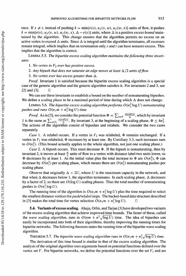
5.4. Variants ofexcess scaling. Ahuja, Orlin, and Tarjan [3] have developed two variantsof the excess scaling algorithm that achieve improved time bounds. The faster of these, calledthe wave scaling algorithm, runs in O(nm + n2v/log U) time. The idea of bipushes caneasily be incorporated into both of their algorithms, thereby improving the running times forbipartite networks. The following theorem states the running time of the bipartite wave scalingalgorithm.

THEOREM 5.7. The bipartite wave scaling algorithm runs in O(n m + nv/iog U) time.

The derivation of this time bound is similar to that of the excess scaling algorithm. Theanalysis of the original algorithm uses arguments based on potential functions defined over thevertex set V. For bipartite networks, we define the potential functions over the set V1 and are

Dow

nloa

ded

05/1

4/18

to 1

29.1

70.1

16.2

35. R

edis

trib

utio

n su

bjec

t to

SIA

M li

cens

e or

cop

yrig

ht; s

ee h

ttp://

ww

w.s

iam

.org

/jour

nals

/ojs

a.ph

p


able to replace n by n in the running time. The detailed proof of this theorem is quite lengthybut contains no new ideas; therefore we omit it. A similar improvement can be obtained inAhuja, Orlin, and Tarjan’s less efficient algorithm, called the stack scaling algorithm.

5.5. Dynamic trees. In the previous four sections, we reduced the time needed to com-pute a maximum flow by reducing the number of nonsaturating pushes. In this section, weconsider a different approach: we reduce the time spent per nonsaturating push. The idea is touse a sophisticated data structure in order to push flow along a whole path in one step, ratherthan pushing flow along a single edge. The dynamic tree data structure of Sleator and Tarjan[34], [33], [37] is ideally suited for this purpose.

The dynamic tree data structure allows the maintenance of a collection of vertex-disjointrooted trees, each edge of which has an associated real value. We adopt the convention thattree edges are directed towards the root. We denote the parent of v by p(v) and regard eachvertex as an ancestor and descendent of itself. We call a dynamic tree trivial if it contains onlyone Va-vertex and nontrivial otherwise. The data structure supports the operations in Fig. 5.2.It is shown in [34] that if the maximum number of vertices in any tree is k, we can perform anarbitrary sequence of tree operations in O (l log k) time.

make-tree(v)find-root(v)find-size(v)find-value(v)

find-min v

change-value(v, z)link(v, w, x)

cut(v)

Make vertex v into a one-vertex dynamic tree.Return the root of v’s tree.Return the number of vertices in v’s tree.Return the value of the tree edge from v to its parent.

Return cz if v is a root.Return the ancestor w of v with minimumfind-value(w).

In case of a tie, choose the w closest to the root.Choose v if v is the root.

Add z to the value of every edge from v to find-root(v).Combine the trees containing v and w by making w the parent

of v and giving edge (v, w) the value x. Do nothing if v and to arein the same tree or if v is not a root.

Break v’s tree into two trees, by deleting the edge joiningv and v’s parent. Do nothing if v is a root.

FIG. 5.2. Dynamic tree operations.

In maximum flow algorithms, the dynamic tree edges are a subset of the current edges.The value of a tree edge is its residual capacity. We maintain the invariant that every activevertex is a dynamic tree root. For this section, we relax the invariant that all excess is onvertices in V and allow excess to accumulate on vertices in V2.

The key to the dynamic tree implementation is the tree-push/relabel operation in Fig. 5.3.The operation is applied to an active vertex v. If there is an eligible edge (v, w) then theoperation adds (v, w) to the forest of dynamic trees, pushes as much flow as possible fromv to the root of the tree containing w, and then deletes from the forest all edges which aresaturated by this push. Otherwise, v is relabeled and its children are cut off. We refer to theoperation of pushing flow from a node of a dynamic tree to the root as a tree-push.

The first dynamic tree algorithm we consider is just the generic preflow-push algorithmwith the push/relabel operation replaced by the tree-push/relabel operation of Fig. 5.3. Wemodify the initialization so that each vertex is in its own one-vertex dynamic tree and we adda post-processing step which extracts the correct flow on each edge that remains in a dynamictree. We call this algorithm the generic bipartite dynamic tree algorithm.

The correctness of this algorithm is straightforward to verify (see [15] and [16]). Weshow that this implementation yields an efficient algorithm.

Dow

nloa

ded

05/1

4/18

to 1

29.1

70.1

16.2

35. R

edis

trib

utio

n su

bjec

t to

SIA

M li

cens

e or

cop

yrig

ht; s

ee h

ttp://

ww

w.s

iam

.org

/jour

nals

/ojs

a.ph

p

IMPROVED ALGORITHMS FOR BIPARTITE NETWORK FLOW 9 17

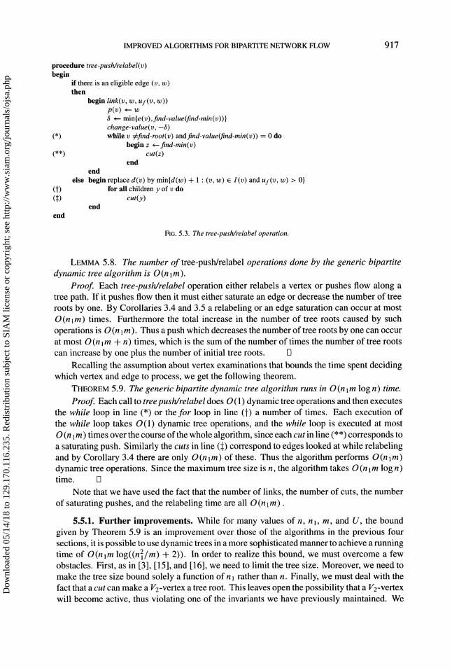
procedure tree-push/relabel vbegin

if there is an eligible edge (o, w)then

begin link(v, w, uf(v, w))p(v) -- w, -- min{e(v),find-value(find-min(v))change-value(v, -,

(*) while v find-root(v) andfind-value(find-min(v)) 0 dobegin z find-min(v)

(**) cut(z)end

endelse begin replace d(v) by min{d(w) + (v, w) I(v) and uf(v, w) > 0}

(]t) for all children y of v do(:) cut(y)

endend

FIG. 5.3. The tree-push/relabel operation.

LEMMA 5.8. The number of tree-push/relabel operations done by the generic bipartitedynamic tree algorithm is 0 (n m).

Proof. Each tree-push/relabel operation either relabels a vertex or pushes flow along atree path. If it pushes flow then it must either saturate an edge or decrease the number of treeroots by one. By Corollaries 3.4 and 3.5 a relabeling or an edge saturation can occur at most

O(nlm) times. Furthermore the total increase in the number of tree roots caused by suchoperations is O (n m). Thus a push which decreases the number of tree roots by one can occurat most O(nlm -t- n) times, which is the sum of the number of times the number of tree rootscan increase by one plus the number of initial tree roots, rq

Recalling the assumption about vertex examinations that bounds the time spent decidingwhich vertex and edge to process, we get the following theorem.

THEOREM 5.9. The generic bipartite dynamic tree algorithm runs in O(nlm log n) time.

Proof Each call to tree push/relabel does O (1) dynamic tree operations and then executesthe while loop in line (*) or the for loop in line (f) a number of times. Each execution ofthe while loop takes O(1) dynamic tree operations, and the while loop is executed at mostO (n m) times over the course of the whole algorithm, since each cut in line (**) corresponds toa saturating push. Similarly the cuts in line (:) correspond to edges looked at while relabelingand by Corollary 3.4 there are only O(nlm) of these. Thus the algorithm performs O(nlm)dynamic tree operations. Since the maximum tree size is n, the algorithm takes O(nlm log n)time. [3

Note that we have used the fact that the number of links, the number of cuts, the numberof saturating pushes, and the relabeling time are all O(nlm).

5.5.1. Further improvements. While for many values of n, n 1, m, and U, the boundgiven by Theorem 5.9 is an improvement over those of the algorithms in the previous foursections, it is possible to use dynamic trees in a more sophisticated manner to achieve a runningtime of O(nlm log((n21/m) + 2)). In order to realize this bound, we must overcome a fewobstacles. First, as in [3], [15], and [16], we need to limit the tree size. Moreover, we need tomake the tree size bound solely a function of n rather than n. Finally, we must deal with thefact that a cut can make a V2-vertex a tree root. This leaves open the possibility that a V2-vertexwill become active, thus violating one of the invariants we have previously maintained. We

Dow

nloa

ded

05/1

4/18

to 1

29.1

70.1

16.2

35. R

edis

trib

utio

n su

bjec

t to

SIA

M li

cens

e or

cop

yrig

ht; s

ee h

ttp://

ww

w.s

iam

.org

/jour

nals

/ojs

a.ph

p


see no way to avoid this--instead we control how this happens and use a fairly complicatedanalysis to show that we can achieve the desired time bounds.

To ensure that the tree size is a function of n and not n, we use the following.LEMMA 5.10. Ifall the leaves in a nontrivial dynamic tree are Vl-vertices, then the number

ofvertices in the tree is at most twice the total number of V1-vertices in the tree.

Proof. Since no V2-vertex is a leaf, all V2-vertices have at least one child. The graph isbipartite, which means that all these children must be Vl-vertices. Therefore, the total numberof V1 vertices in the tree must be at least as large as the total number of V2-vertices. q

We will use two rules to enforce this invariant. First, if a link operation could make a

Ve-vertex a leaf, we do not perform that link. This rule will be respected in all the proceduresthat follow. Second, if a cut causes a V2-vertex to become a leaf, we immediately cut thatvertex from the tree. This idea is implemented in procedure bi-cut, which appears in Fig. 5.4.Procedure bi-cut will be used in place of cut. Observe that procedure bi-cut performs at mosttwo dynamic tree operations.

procedure bi-cut(begin

if vthen cut(p(v))cut(v)

end

FIG. 5.4. The bi-cut operation.

We also want to maintain the invariant that no tree have more than k vertices (k will bechosen later). As in [15] and [16] we achieve this by preceding each link operation by acalculation of whether or not the result of the link will be a tree of greater than k vertices. Ifso, we do not perform the link. Since trees only grow as the result of link operations, it is clearthat this maintains the desired invariant.

The main problem left to address is the complexity added by allowing excess to remain on

V2-vertices. In general, this yields slower running times. We maintain the following invariant,however.

INVARIANT 5.11. Whenever a V2-vertex is relabeled, it does not have any excess on it.

As we shall see, this will allow us to get a good bound on the number of tree operations.To maintain this invariant we need to ensure that we always have the flexibility to send all

the excess from a V2-vertex out over the current edge. The following lemma gives a conditionsufficient to guarantee this flexibility.

LEMMA 5.12. Let out-cap(v) be the residual capacity of the current edge of v. lffor all

V2-vertices v that are dynamic tree roots, we maintain that

(5.1) e(v) < out-cap(v)

and that the current edge of v is eligible, then lnvariant 5.11 can be satisfied with O(1)additional work per tree-push or relabeling operation.

Proof The left side of (5.1) can change when we do a push that involves v, and the rightside can change when the current edge of v changes. We deal with these two cases separately.When doing a tree-push that terminates at a root r that is a V2-vertex we must ensure that thenew excess does not exceed out-cap(r). To do this we simply push less flow. This idea is

captured in a new procedure called bi-send, which appears in Fig. 5.5. This procedure will beused whenever we want to push flow along a path from a tree vertex to the root.

Dow

nloa

ded

05/1

4/18

to 1

29.1

70.1

16.2

35. R

edis

trib

utio

n su

bjec

t to

SIA

M li

cens

e or

cop

yrig

ht; s

ee h

ttp://

ww

w.s

iam

.org

/jour

nals

/ojs

a.ph

p


procedure bi-send(v)begin

f .--find-root(v)if r VIthen

+-- min{e(v),find-value(find-min(v))}else

(*) min{e(v), find-value(find-min(v)), out-cap(r) e(r)change-value(v, -3)while v ’=find-root(v) andfind-value(find-min(v)) 0 do

begin z -- find-min(v)bi-cut(z)end

end

FIG. 5.5. The bi-send operation.

Next we have to deal with the case when out-cap(v) changes. Let (v, w) be the currentedge of v. The value of out-cap(v) may change in two different ways. One way is that (v, w)may become saturated. When this happens, invariant (5.1) implies that the push saturating(v, w) rids v of all its excess. After the push, we advance the current edge pointer of v tothe next eligible edge, doing a relabeling if necessary. The second case is that w may berelabeled, thus making (v, w) ineligible. The current edge pointer of v is advanced to thenext eligible edge; for this new edge, (5.1) may be violated, however. To handle this case,we always push flow over edge (v, w) before relabeling w. This change is summarized inprocedure bi-relabel(w), which appears in Fig. 5.6. Observe that since all edges incident tow must be inspected in order to relabel w, procedure bi-relabel runs in the same asymptotictime as procedure relabel.

procedure bi-relabel(w)begin

ifw V1then for all v s.t. the current edge of v is (v, w) do

push e(v) units of flow over edge (v, w)replace d(v) by min{d(w) + (v, w) I(v) and uf(v, w) > O}for all children y of v do

bi-cut(y)end

FIG. 5.6. The bi-relabel operation.

What we have shown is that whenever the current edge pointer of w V2 advances, thereis no excess at w. Since this pointer advances to the end of the list before arelabel, it mustbe true that at the time of a relabel there is no excess on w. Further, the only algorithmicchanges are the change in line (*) of bi-send, which adds O(1) work per tree push, the changein bi-relabel, which adds O(1) work per relabel, and a change in the current edge advancementprocedure, to make sure that current edges from V2-vertices are always eligible.

Given these building blocks we can give the procedure bi-tree push/relabel, which incor-porates all of these ideas. The procedure appears in Fig. 5.7. The basic idea is similar to thatused in [3], [15], and [16], in that we do a tree-push, but only perform a link if the size of theresulting tree is not too large. We also have the additional constraint of not performing a linkthat will cause a V2-vertex to become a leaf. This leads to lines (T1) through (T2) of bi-treepush/relabel which handle the case when we are pushing from a trivial dynamic tree. In thiscase we first push flow over v’s eligible edge (v, w). Then we do a bi-send(w) and proceed asif we had started at the root of w’s dynamic tree. We also make one technical change and usea procedure called bi-send* instead of bi-send in line (TB). Procedure bi-send* differs from

Dow

nloa

ded

05/1

4/18

to 1

29.1

70.1

16.2

35. R

edis

trib

utio

n su

bjec

t to

SIA

M li

cens

e or

cop

yrig

ht; s

ee h

ttp://

ww

w.s

iam

.org

/jour

nals

/ojs

a.ph

p


bi-send in that it defers doing its cuts until line (**) of procedure bi-tree push/relabel. This isdone in order to avoid the case that the link performed in line (f) is linking a trivial dynamictree, as this would make a V2-vertex a leaf. (This is done purely for ease of presentation andis not necessary.)

procedure bi-tree-push/relabe vbegin

if there is an eligible edge (v, w)(T1) then begin if v is a trivial V2 tree

then begin push flow on edge (v, w)r -- find-root(w)(TB) bi-send*(w)if there is an eligible edge (r, q)then begin v r

w--qend

else bi-relabel(r)(T2) end

iffind-size(v) +find-size(w) < k(f) then begin link(v, w, uf(v, w))

p(v) +-- wend

(*) else begin push flow on edge (v, w)bi-send(w)

(**) Perform the cuts from line (TB) (there may be none)end

end

elseend

bi-relabel(v)

FIG. 5.7. The bi-tree-push/relabel procedure.

We now use procedure bi-tree-push/relabel in a FIFO algorithm. We call this the FIFObipartite dynamic tree algorithm.

Since, by Invariant 5.11, whenever a V2-vertex is relabeled it has no excess, we can derivea bound of O(n2) passes over the queue, by a proof similar to that of Lemma 5.1. Define avertex activation to be the event that either a vertex with zero excess receives positive excess,or a vertex with positive excess is relabeled. This corresponds to a vertex being placed on thequeue. We will need to bound the number of times this occurs.

First, we give a lemma, the proof of which is simliar to that of Lemma 5.8 and Theorem5.9, with the additional observation that the time spent in an iteration of bi-tree-push/relabelis within a constant factor of the amount of work done by tree-push/relabel.

LEMMA 5.13. The FIFO bipartite dynamic tree algorithm runs in 0 (n m log k) time plusO(log k) time per vertex activation.

All that remains is to bound the number of vertex activations. First we introduce someterminology. We denote the tree containing vertex v by To. We call a tree large if the numberof nodes in the tree is at least k/2. As a consequence of Lemma 5.10, there are only 2nlvertices in all the nontrivial dynamic trees, hence there are no more than 4nl/k large trees atany time. In particular we will use the fact that there are O (n / k) large trees at the beginningof a pass over the queue.

LEMMA 5.14. The number of vertex activations is O(nlm + n/k).Proof. By Invariant 5.11, all Vz-vertices have zero excess when relabeled, thus the only

vertex activations due to relabelings are from V-vertices. There are at most O(n) of these.

Dow

nloa

ded

05/1

4/18

to 1

29.1

70.1

16.2

35. R

edis

trib

utio

n su

bjec

t to

SIA

M li

cens

e or

cop

yrig

ht; s

ee h

ttp://

ww

w.s

iam

.org

/jour

nals

/ojs

a.ph

p


There can be only O (nlm) vertex activations for which the corresponding bi-tree-push/relabelexecutions perform a cut or link or a saturating push in line (*).

it remains to count the vertex activations for which the corresponding invocation of bi-tree-push/relabel does neither a cut nor a link nor a saturating push. If this occurs then it mustbe thatfind-size(v) +find-size(w) > k, i.e., either To or To is large. We consider the two casesseparately.

Suppose To is large. Vertex v is the root of To. Since the push is nonsaturating, it mustrid v of all its excess. If To has changed since the beginning of the current pass, we chargethe activation to the link or cut that most recently changed To. This occurs at most once percut and twice per link for a total of O(n m) time overall. If To has not changed since thebeginning of the pass, we charge the activation to Tv. There are at most O(n/k) large treesat the start of a pass, hence this case counts for O(n/k) charges overall.

Suppose To is large. In this case the root r of To may be added to the queue. As before,if To changed during the pass we charge the activation to the link or cut which caused it,otherwise we charge it to the large tree.

We have ignored so far the possible activations in lines (T1) through (T2). It is easy toverify that these only add a constant factor to the bounds mentioned above. The reason foradding this case is to ensure that in every iteration either a link, cut, or saturation is performed,or a large tree is involved. This additional case allows us to ensure this with no asymptoticloss in the running time of the procedure.

Combining all these cases we get O(nm + n3/k) vertex activations.THEOREM 5.15. The FIFO bipartite dynamic tree algorithm runs in O(nm log((n/m)

2)) time.

Proof Apply Lemmas 5.13 and 5.14 and choose k (n/m) + 2.

5.11. A parallel implementation. In this section, we give a parallel implementationof the bipartite excess scaling algorithm. Our model of computation is an exclusive-readexclusive-write parallel random access machine (EREW PRAM) [13]. Our algorithm runs inO((nm)/d + n log U) log d) time using d [n’l processors, thus achieving near-optimalspeedup for the given number of processors. We assume familiarity with parallel prefixoperations [22] and refer the reader to [2], [16], [26], and [32] for examples of the use ofparallel prefix operations in network flow algorithms. Specifically, we use the fact that usingd processors and O (log d) time, we can execute the following parallel prefix operation:

Parallel Prefix Operation: Given/< d numbers f(v) f(vt), computethe partial sums f(v), f(v) + f(v2) f(Vl) +... -+- f(Vl).

Our algorithm will be the same as the excess-scaling algorithm of 5.3 with a parallel im-plementation of bipush/relabel and a few additional data structures. The same approach wastaken by Ahuja and Orlin [2] in developing a parallel version of their original excess scalingalgorithm.

The first step in our algorithm is to transform the input graph so that each vertex has out-degree no greater than d. This transformation yields a graph with O(n) V-vertices, O(n2)Vz-vertices and O(m) edges. We achieve this by repeating the following step until it is no

longer applicable:

splitting step: Pick a vertex v with out-degree k > d. Create two new ver-tices v’ and v" andreplace edges (v, vk-a+)... (v, vk) withedges (v, v’), (v’, v"),and (v", vk-a+)... (v", vk). Edges (v, v’) and (v’, v") have infinite capac-ity, while each edge (v", vk) has its capacity set equal to u(v, vk).

Dow

nloa

ded

05/1

4/18

to 1

29.1

70.1

16.2

35. R

edis

trib

utio

n su

bjec

t to

SIA

M li

cens

e or

cop

yrig

ht; s

ee h

ttp://

ww

w.s

iam

.org

/jour

nals

/ojs

a.ph

p


The splitting step creates one new V-vertex, one new Vz-vertex, and 2 more edges. Leto max{0, [(out-degree(v) d)/(d 1)]}. Each splitting step reduces by one. Initially

O(n 1) and > 0 when the algorithm terminates. Thus, we only need to perform thesplitting step O(n) times overall, adding O(n) vertices and O(n) edges. Similarly, we canrepeat the same step to reduce the in-degree of each vertex.

Further, we can perform this step in O(n log m) time on d processors. We explainhow to reduce the in-degree; the out-degree can be reduced in a similar manner. First, welexicographically sort the list of edges by their tails. This can be done on d processors inO(n log m) time using Cole’s sorting algorithm [8] and Brent’s theorem [6]. Next, we assignone processor to each of the last d edges on the list. In O (log d) time, we can determine if allthese edges have the same tail. If so, we perform the splitting step, which can be done in O (1)time on d processors. We then delete these edges from the list and continue on the remainderof the list. If they do not all have the same tail, then the last vertex on the list must have degree< d. In this case we delete all edges which have the same tail as the last edge and continue onthe remainder of the list. In each iteration we either delete all the edges incident to a vertex

mor we process d edges. Hence there are O(n + 7) O(n) iterations, each of which can beperformed in O (log m) time on d processors.

For the rest of this section, we will assume, without loss of generality, that every vertexin our graph has both in-degree and out-degree < d.

We first address the problem of implementing a bipush in parallel. In the bipush operationfor the maximum flow problem, it is necessary to scan the edge list for vertex v starting withthe current edge for vertex v until either an eligible edge is determined or until the edge list isexhausted. In the parallel algorithm, we will scan these edges in parallel.

We begin by introducing some terminology. Let I(v) denote the set of vertices w suchthat (v, w) is an edge, and let (v) denote the set of vertices w such that (v, w) is an eligibleedge. Let us assume that the vertices in I(v) are denoted v, 1)2 Ok, where k II(v)l.Thus the jth edge emanating from vertex v is edge (v, vj).

For each vertex v 6 V2, we let (v) wo) r(v, w), and refer to (v) as the effectiveresidual capacity of vertex v. Note that we can always push all of the excess out of a vertexv in V2 prior to a relabeling of v so long as the excess does not exceed the effective residual

capacity.We define the effective residual capacity (v, w) of edge (v, w) as

0 if (v, w) is not eligible,(v, w) r(v, w) if (v, w) is eligible and v 6 V2, w 6 V,

min{r(v, w), (w)} if (v, w) is eligible and v 6 V, w 6 V2.

In the algorithm, we will be performing pushes from one vertex in V at a time, andwe will subsequently push from several vertices in V2 in parallel. By defining the effectiveresidual capacity for edges (v, w) as we do, we will ensure that we never push more flow into

any vertex v 6 V2 than the effective residual capacity of v. Subsequently, all of the flow canbe pushed out prior to a relabel of v.

In order to achieve the speedup desired, we cannot assign one processor to each edgeof I(v) in a push from vertex v. Thus, we will have to more efficiently allocate processorsto edges on which we wish to push flow. In order to do so, we introduce the following fourprocedures. In all these procedures v is a vertex from which we wish to push 6 units of flow.

We use Current(v) to denote v’s current edge and store the edge lists in arrays.1. NextCurrent(v, 3)" if pushing 3 units of flow would saturate all of v’s admissible

edges, then output I(v)] + 1. Otherwise, output the index of the edge that will be current

after pushing 3 units of flow from v.

Dow

nloa

ded

05/1

4/18

to 1

29.1

70.1

16.2

35. R

edis

trib

utio

n su

bjec

t to

SIA

M li

cens

e or

cop

yrig

ht; s

ee h

ttp://

ww

w.s

iam

.org

/jour

nals

/ojs

a.ph

p


2. NewRelabel(v, 3)" output true ifNextCurrent (v, 3) II(v)l + and false otherwise.3. NextIncrement(v, 3)" output the amount of flow that will be sent in edge

NextCurrent(v, 3) when pushing flow from v.

4. Requirement(v, 3)" output the number of edges scanned in order to send 3 units offlow from v without a relabel. It is equal to NextCurrent (v, 3) Current (v) + 1.

LEMMA 5.16. There exists a data structure that allows us to implement each of theseoperations in 0 (log d) time on one processor.

We defer the proof until later. Assume for now that such an implementation exists.

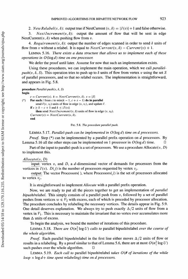
Using these procedures, we can implement the main operation, which we call parallel-push(v, 3, S). This operation tries to push up to units of flow from vertex v using the set Sof parallel processors, and so that no relabel occurs. The implementation is straightforward,and appears in Fig. 5.8.

procedure Parallel-push(v, 3, S)begin

c Current(v). k NextCurrent(v, 3). s ISI(*) For each from c to min(k 1, c + s 1) do in parallel

send (v, vi) units of flow in edge (v, vi), and update .ifs > k-c + andk < II(v)l

then send Nextlncrement(v, 3) units of flow in edge (v, v-).Current(v) NextCurrent(v, 3).end

FIG. 5.8. The procedure parallel push.

LEMMA 5.17. Parallel-push can be implemented in O(log d) time on d processors.

Proof Step (*) can be implemented by a parallel prefix operation on d processors. ByLemma 5.16 all the other steps can be implemented on processor in O (log d) time.

Part of the input to parallel-push is a set of processors. We use a procedure Allocate(v, D)to implement this.

Allocate(v, D)input: vertex v, and D, a d-dimensional vector of demands for processors from the

vertices in I (v). D(j) is the number of processors requested by vertex vj.output: The vector Processors(), where Processors(j) is the set of processors allocated

to vertex vj.

It is straightforward to implement Allocate with a parallel prefix operation.Now, we are ready to put all the pieces together to get an implementation of parallel

bipush/relabel. This simply consists of a parallel push from v, followed by a set of parallelpushes from vertices w 6 V2 with excess, each of which is preceded by processor allocation.The procedure concludes by relabeling the necessary vertices. The details appear in Fig. 5.9.One detail deserves explanation. We always try to push exactly A/2 units of flow from avertex in V. This is necessary to maintain the invariant that no vertex ever accumulates morethan A units of excess.

To begin the analysis, we bound the number of iterations of this procedure.LEMMA 5.18. There are O(n2 log U) calls to parallel bipush/relabel over the course of

the whole algorithm.

Proof Each parallel bipush/relabel in the first line either moves A/2 units of flow orresults in a relabeling. By a proof similar to that of Lemma 5.6, there are at most O (n2 log U)such pushes over the whole algorithm.

LEMMA 5.19. Each call to parallel bipush/relabel takes 0(# of iterations of the whileloop log d+ time spent relabeling) time on d processors.

Dow

nloa

ded

05/1

4/18

to 1

29.1

70.1

16.2

35. R

edis

trib

utio

n su

bjec

t to

SIA

M li

cens

e or

cop

yrig

ht; s

ee h

ttp://

ww

w.s

iam

.org

/jour

nals

/ojs

a.ph

p


procedure parallel bipush/relabel(v)begin

Parallel push(v, A/2, d)while e(vj) = 0 for some vj I (v) dobegin

for each to d do in parallelD(vj) Requirement(vj, e(vj)).

Allocate(v, D, d).for to d do in parallelbegin

(*) push(vi, e(vi), processors(i)).update data structures.

endendcreate a list L of indices j s.t. j V2 and NewRelabel(vj) true.for each L do Relabel(vi).if NewRelabel(v) true then relabel(v).

end

FIG. 5.9. Procedure parallel bipush/relabel.

Proof By Lemma 5.16 and the fact that Allocate takes O(log d) time, each step exceptfor the parallel push in line (*) takes O(log d) time. We know from Lemma 5.17 that a pushtakes O (log d) time. It is easy to see that a set of pushes which use a total of d edges can alsobe completed in O(log d) time; thus each iteration of the while loop takes O(log d) time. Thelemma follows. [3

It remains to bound the number of iterations of the while loop.LEMMA 5.20. The while loop is executed O((n m/d) + n log U) times over the whole

algorithm.

Proof. First we observe that each vertex in I (v) may have at most one nonsaturating pushfrom it per execution of the while loop. Lemma 5.18 implies that the number of nonsaturatingpushes is at most O(nZd log U) overall. Let nsp be the number of nonsaturating pushesthat have occurred since the beginning of the algorithm. Consider the potential function Fv current (v) + nsp. Initially F 0 and at termination F (# of nonsaturating pushes)O(nd log U). The only way for F to decrease is by a relabel. Each relabel decreases F byat most II(v)l; the total decrease is O(nlm). So, the total increase in F over the algorithmis O((nd log U + n lm)). A parallel push with k processors increases F by k or results in arelabeling. Each iteration in a while loop except for the last one allocates d processors; henceit increases F by d or results in a relabeling. Ignoring the last iteration of the while loop in eachcall to parallel bipush/relabel, we find that there are at most O((nd log U+nlm)/d) iterationsof the while loop. To count the last iterations, we observe that there is one last iteration per

(nlmcall for a total of O(n log U) Thus, overall there are O,--d- + n log U) iterations 1

LEMMA 5.21. The total time spent relabeling is O(((nlm/d) + n log U) log d).

Proof We spend a total of O(n m) work relabeling. However, at each relabeling stepwe look at d edges at a time, except for the last relabel step in a call to parallel bipush/relabel.

(nlmHence the total time is O -d-- + n log U) [3

Now we turn to the proof of Lemma 5.16.

Proof (of Lemma 5.16). Assume for now that k II(v)l is a power of 2 for each vertex.We create a complete binary tree whose leaves are the indices of the vertices in I(v). The keyof each leaf j in the binary tree is (v, vj). The key of each internal vertex of the binary treeis the sum of the keys of its descendent leaves.

Dow

nloa

ded

05/1

4/18

to 1

29.1

70.1

16.2

35. R

edis

trib

utio

n su

bjec

t to

SIA

M li

cens

e or

cop

yrig

ht; s

ee h

ttp://

ww

w.s

iam

.org

/jour

nals

/ojs

a.ph

p


Whenever a vertex v is relabeled, each vertex vj of I(v) is assigned a processor, andits binary tree is updated. The assignment of processors takes O(log d) steps per relabel.Moreover, each processor updates its binary tree in O (log d) steps.

When a push from vertex v is performed, the binary tree for vertex v must be updated.If k processors are assigned then Current(v) is increased by < k, and the updating can beaccomplished with k processors in O(log d) time.

In order to compute NextCurrent (v, ), we start at the root of the binary tree for v,and we select the right child or the left child depending on whether 6 is less than or greaterthan the key of the right child. We then recur on the selected child. We also can computeNextIncrement in this manner. 71

Combining all the above results, we have the following theorem.THEOREM 5.22. Algorithm Bipartite Excess Scaling with bipush/relabel replaced by

parallel bipush/relabel runs in O(((nlm/d) + n log U)log d) time on d processors on anEREW PRAM.

Plugging in d [], we can restate the theorem as the following corollary.COROLLARY 5.23. Algorithm Bipartite Excess Scaling with bipush/relabel replaced by

parallel bipush/relabel runs in O(n2 log U log ) time on processors on an EREWPRAM.The work done by this algorithm is within a logarithmic factor of the running time of the

sequential bipartite excess scaling algorithm.

6. Parametric maximum flow. A natural generalization of the maximum flow problemis obtained by making the edge capacities functions of a single parameter .. This problemis known as the parametric maximumflow problem. We consider parametric maximum flowproblems in which the capacities of the edges out of the sink are nondecreasing functions of,k, the capacities of the edges into the sink are nonincreasing functions of ., and the capacitiesof the remaining edges are constant. Although this type of parameterization appears to bequite specialized, Gallo, Grigoriadis, and Tarjan [14] have pointed out that this parametricproblem has many applications, in computing subgraph density and network vulnerability andin solving other problems, some of which are mentioned at the end of this section.

Let uz (v, w) denote the capacity of edge (v, w) as a function of ,k and suppose that wewish to solve the maximum flow problem for parameter values 1 _< 2 < < ,l. Clearly,for different values of ,k, a solution can be found using invocations of a maximum flowalgorithm. This approach takes no advantage of the similarity of the successive problems tobe solved, however. Gallo, Grigoriadis, and Tarjan [14] gave an algorithm for finding themaximum flow for O(n) increasing values of . in the same asymptotic time that it takes torun the Goldberg-Tarjan maximum flow algorithm once. If the capacities are linear functionsof ,k, it is easy to show that the value of the maximum flow, when viewed as a function of ),is a piecewise linear function with no more than n 2 breakpoints. In this case, they give analgorithm for finding all of the breakpoints of this function in the same asymptotic time as ittakes to run the Goldberg-Tarjan maximum flow algorithm once.

In this section we give an algorithm which for increasing values of k finds all maximumflows in O(ln + ln2 + n3 + nm) time. Using the dynamic tree data structure, this algorithmruns in O(ln + nm log((ln + nZ)/m + 2)) time.

We begin by giving one iteration of the algorithm, i.e., determining the maximum flowfor parameter value ,ki, if the maximum flow for parameter value ,ki_ is given. The algorithmappears in Fig. 6.1. First, we update the capacities. The capacity of an edge leaving the sourcemay have increased. If so, we saturate the edge, by setting its flow equal to its new capacity.The capacity of an edge leaving the sink may have decreased. If it has decreased below theflow on the edge, we decrease the flow so that it is equal to the capacity. Since 6 V1 by

Dow

nloa

ded

05/1

4/18

to 1

29.1

70.1

16.2

35. R

edis

trib

utio

n su

bjec

t to

SIA

M li

cens

e or

cop

yrig

ht; s

ee h

ttp://

ww

w.s

iam

.org

/jour

nals

/ojs

a.ph

p


assumption, this may create excess on vertices in V2. Therefore, we immediately push anysuch excess to vertices in V, thus re-establishing the invariant that no excess is on vertices in

V2. The second step consists of running the bipartite FIFO algorithm in the network beginningwith the current f and d. This gives us a maximum flow for the parameter value

Step (Update preflow)Let +(s, v) 6 E with d(v) < 2Hi, let f(s, v) max{uzi (s, v), f(s, v)}.(v, t) E, let f(v, t) min{ux; (v, t), f(v, t)}.’v V2 while e(v) > 0, do push/relabel(v).

Step 2 (Find maximum flow) Run the bipartite FIFO algorithm on the network with capacities u beginningwith flow f and distance labels d.

Fl6. 6.1. Algorithm parametric bipartite flow.

Remark. In applications of the parametric maximum flow problem, it may happen thats 6 V or 6 V2, contrary to our assumption. Such a possibility can be handled by makingminor changes to the algorithm, without affecting its running time.

Now we must prove that the algorithm is correct and efficient. We do this by means ofthe following lemmas.

LEMMA 6.1. At the end of each step in the algorithm, there is no excess on any vertexin V2.

Proof. It suffices to restrict our attention to Step 1, since Step 2 always maintains thiscondition. Since by assumption s 6 V2, increasing the flow on edges out of s can increase theexcess only on vertices in V. Since 6 V2, decreasing the flow on edges into may createexcesses on vertices in V2. This excess is immediately removed from vertices in V2 by theprocedure push/relabel, however. [3

LEMMA 6.2. Throughout all iterations ofthe parametric bipartite flow algorithm, distancelabels are nondecreasing.

Proof. We first show that updating the residual capacities and the preflow between itera-tions maintains the validity of the distance labels. Increasing the flow on an edge (s, v) maycreate a new residual edge (v, s), but since d(v) < 2nl, the labeling is still valid. Decreasingthe flow on edges into does not create any new residual edges, so the distance labels arestill valid. We noted earlier that procedures push/relabel and bipush/relabel maintain a validlabeling. The lemma follows.

A consequence of Lemma 6.2 is that, over all iterations of the algorithm, each vertexis relabeled O(nl) times, and the total relabeling time is O(nlm). Furthermore, the totalnumber of saturating pushes over the whole algorithm is O (nm). We bound the number ofnonsaturating bipushes in the next lemma.

LEMMA 6.3. The algorithm performs a total of O(ln + n) nonsaturating bipushes overall iterations.

Proof. As in the bipartite FIFO algorithm, consider the following potential function:max{d(v)lv is active}. The potential function increases due to relabelings, and this

increase has already been shown to be at most 4n2. The potential function may also increasein Step when the preflow is updated. But this increase is at most O(nl) per iteration, andO(nl) over all iterations. Thus the total number of passes over the queue is O(ln + n21) andthe total number of nonsaturating bipushes is O(ln2 + n). [3

THEOREM 6.4. A total of iterations of the parametric bipartite flow algorithm takeO(ln + nm + ln + n3) time.

Proof. Each execution of Step takes O(n) time to update the residual capacities andflows. Getting rid of the excesses at vertices in V2 by performing push/relabel steps takes

Dow

nloa

ded

05/1

4/18

to 1

29.1

70.1

16.2

35. R

edis

trib

utio

n su

bjec

t to

SIA

M li

cens

e or

cop

yrig

ht; s

ee h

ttp://

ww

w.s

iam

.org

/jour

nals

/ojs

a.ph

p


O(n) time per iteration plus the time to perform saturating pushes, which is O(n m) timeoverall. Hence executions of Step take O(ln + nlm) time. The executions of Step 2 takea total of O(nlm + ln2 + n) time, as was shown previously. The theorem follows.

The dynamic tree data structure can be incorporated into the parametric maximum flowalgorithm to improve its computational complexity. Using the ideas described in 5.5, it canbe shown that the dynamic tree implementation of the parametric maximum flow problemruns in O(ln + nlm log((lnl + nZ)/m + 2)) time.

Often applications of the parametric maximum flow problem require that the minimum cutbe determined for each of the parameter values .l, )2 ,l. Obviously each such minimumcut can be determined by a breadth-first search of the network, requiring O (m) effort per cut.Overall this time would be O(ml) and for larger values of would be a bottleneck. In order toachieve a faster time bound we maintain exact distance labels of vertices as explained in 16].Maintaining exact distance labels requires some additional effort but no more than O(ntime over all iterations. While using this method, the minimum cut (Xi, Xi), at the end ofiteration/is defined as X {1) E V d(v) > 2nl} and X {1) V d(v) < 2nl}. It mayalso be pointed out the minimum cuts in the parametric maximum flow problem are nested,i.e., for Zl < 2 < .3, with corresponding cuts (X1, X1), (X2, X2), (X3, X3), we have thatX1 c_ X2 __. X3 12]. This property allows us to store all cuts in O(n + l) space, and recreateany one cut in O (n) time.

While we have only given an algorithm for the case where the ’s are given in increasingorder, actually we can solve a more general problem. Let x(X), the min-cut capacityfunction,be the capacity ofthe minimum cut as a function of,k. If the edge capacities are linear functionsof X, then x(.) is a piecewise-linear concave function with at most n 2 breakpoints. We canactually compute all of these breakpoints in O(n2 + nlm log((nnl/m) + 2)) time, and can doeven better if we know a priori that o(n). This result directly follows from the results of[14] and the details appear in [35].

We conclude by noting that the bipartite parametric flow problem has many applicationsincluding multiprocessor scheduling with release times and deadlines [21 ], [24], 0-1 integerprogramming problems [29], [30], maximum subgraph density [21 ], finding a maximum-sizeset ofedge-disjoint spanning trees in an undirected graph [28], [29], [30], network vulnerability[9], 19], partitioning a data base between fast and slow memory [11], and the sportswriter’send-of-season problem [23], [31]. For all these problems we improve on or match the bestknown bounds.

7. Minimum-cost circulation. In this section we examine the minimum-costflow prob-lem on bipartite networks. We consider the recent cost-scaling minimum-cost flow algorithmof Goldberg and Tarjan 17], and describe the improvement in its running time that can beobtained when it is adapted for bipartite networks. We shall be very sketchy in our description,since all the results are analogous to the results in 5.

The minimum cost flow problem is a generalization of the maximum flow problem. Inthis problem, each edge (v, w) has a cost c(v, w). We formulate the problem as a circu-lation problem, since it is equivalent to other formulations. (See [1] and [18].) We as-sume that the costs are antisymmetric, i.e., c(v, w) -c(w, v) for each edge (v, w). LetC max{c(v, w) (v, w) 6 E}. The minimum-cost circulation problem can be formulatedas follows:

Minimize c(v, w)f(v, w)(v,w)E

subject to

Dow

nloa

ded

05/1

4/18

to 1

29.1

70.1

16.2

35. R

edis

trib

utio

n su

bjec

t to

SIA

M li

cens

e or

cop

yrig

ht; s

ee h

ttp://

ww

w.s

iam

.org

/jour

nals

/ojs

a.ph

p


(7.1) f(v, w) < u(v, w) (v, w) E,

(7.2) f(v, w) -f(w, v) (v, w) E,

(7.3) f(v, w) =O Yv 6 V.wEV

A circulation is a function of satisfying constraints (7.1), (7.2), and (7.3). A pseudoflowis a function f satisfying only constraints (7.1) and (7.2). For any pseudoflow f, we definethe excess of vertex to to be

(7.4) e(w) f(v, w).v:(v,w)EE

The excess at a vertex may be positive or negative. A vertex v is called active if e(v) > O.The residual network is defined as for the maximum flow problem. We associate with eachvertex v a real-valued price p(v). The prices correspond to linear programming dual variables.In the analysis, the prices play a role similar to that played by the distance labels in the maximumflow algorithm. The reduced cost of an edge (v, w) with respect to the price function p isdenoted by Cp(V, w) and is defined by Cp(V, w) c(v, w) + p(v) p(w).

7.1. The cost-scaling algorithm. The cost-scaling algorithm of Goldberg and Tarjan[17], relies on the concept of approximate optimality. A circulation f is said to be e-optimalfor some e > 0 if f together with some price function p satisfies the following condition:

(7.5) uf(v, w) > 0 =, Cp(V, w) >_ -e ==, (e-optimality).

We refer to this condition as the e-optimality condition. Let be the number of edges onthe longest simple cycle in the network. It can be shown that any feasible flow is e-optimalfor e > C and any e-optimal feasible flow for e < 1/l is an optimum flow [4]. Since in abipartite network every other vertex on a cycle must be a vertex in V1, any e-optimal feasibleflow for e < 1/(2nl) is an optimum flow.

The cost-scaling algorithm treats e as a parameter and iteratively obtains e-optimal flowsfor successively smaller values of e. Initially, e C; on termination, e < / (2n ). The algo-rithm performs repeated cost-scaling phases, each of which consists of applying an improve-approximation procedure that transforms a 2e-optimal circulation into an e-optimal circulation.After + [log(2nlC)] cost scaling phases, e < 1/(2nl), and the algorithm terminates withan optimal circulation. To get the algorithm started, an initial circulation can be found byusing any maximum flow algorithm, such as one of those discussed in 5. A more formaldescription of this algorithm appears in Fig. 7.1.

Recall that in the maximum flow algorithm, we maintained the invariant that all excesswas on V-vertices. This will be our goal in the minimum cost circulation algorithm also. Theprocedure improve-approximation given in Fig. 7.2 first converts the 2e-optimal circulation itreceives as input into a 0-optimal pseudoflow (lines (*) through (**)). This may leave positiveexcess on Vz-vertices. So we execute the while loop at line (f), which applies pushoperations to these vertices until they are rid of all their excess. Now we have establishedthe invariant that the only vertices with positive excess are V-vertices. We will maintain thisinvariant for the rest of procedure improve-approximation. The remainder of the proceduremoves flow from vertices with positive excess to vertices with negative excess. As vertices

Dow

nloa

ded

05/1

4/18

to 1

29.1

70.1

16.2

35. R

edis

trib

utio

n su

bjec

t to

SIA

M li

cens

e or

cop

yrig

ht; s

ee h

ttp://

ww

w.s

iam

.org

/jour

nals

/ojs

a.ph

p


algorithm cost scalingbegin

p=0; C;let f be any initial circulation;while > do2n

begin e/2improve-approximation(f, p, );

endend

FIG. 7.1. Algorithm cost scaling.

procedure improve-approximation(f, p, E)begin(*) if Cp(V, w) < 0

then begin f(v, w) u (v, w);f(w,v)=-f(v,w)

end;(**) compute vertex imbalances;(’) while the network contains an active V2-vertex v do

push(:) while the network contains an active vertex v do

bipush/update vend

FIG. 7.2. The procedure improve-approximation.

in V2 may have negative excess, this will sometimes involve a one-edge push and sometimesinvolve a two-edge push.

We call an edge (v, w) in the residual network admissible if Cp(V, w) < 0. We define thesubnetwork ofG consisting solely of admissible edges to be the admissible network. The basicoperations in the procedure are selecting active vertices, pushing flows on admissible edges,and updating vertex prices. The details of improve-approximation, adapted to the bipartitecase, appear in Figs. 7.2 and 7.3.

procedure bipush/update(vbegin

if there exists an admissible edge (v, w)then if e(w) < 0

then push min[e(w), e(v), uf(v, w)} units of flow on (v, w)else if there exists an admissible edge (w, x)

then push 3 min{e(v), uf(v, w), Uf(W,X)} units of flowalong the path v w x

else replace p(w) by max(w,x)eEj.{p(x) c(w, x) e}else replace p(v) by max(v,u,)eEj.{p(w) c(v, w) }

endprocedurepushbegin

if there exists an admissible edge (v, w)then push min{e(w), e(v), uf(v, w)} flow on (v, w)else replace p(v) by max(o,u)Ef {p(w) c(v, w) }

end

FIG. 7.3. The procedures push/update and bi-push/update.

To identify admissible edges emanating from a vertex, the algorithm uses the same current

edge data structure used in the preflow-push algorithm for the maximum flow problem.

Dow

nloa

ded

05/1

4/18

to 1

29.1

70.1

16.2

35. R

edis

trib

utio

n su

bjec

t to

SIA

M li

cens

e or

cop

yrig

ht; s

ee h

ttp://

ww

w.s

iam

.org

/jour

nals

/ojs

a.ph

p


A movement offlow along a path v w -x in bipush/update is called a bipush. The bipushis saturating if 3 min{uf(v, w), uf(w, x)} and nonsaturating otherwise. The correctnessand efficiency of the algorithm rest on the following results.

LEMMA 7.1. 1. The improve-approximation procedure always maintains e-optimality ofthe pseudoflow, and at termination yields an e-optimal circulation.

2. Each vertex price never increases, and it decreases O(n 1) times during an execution

of the procedure.3. There are 0 (n m) saturatingpushes andbipushes during an execution oftheprocedure.4. Immediately before, during, and immediately after the while loop in line () ofimprove-

approximation, all excess is on V-vertices.Proof These results follow directly from the proofs of Goldberg and Tarjan 17] adapted

for bipartite networks. E]

As in the preflow-push algorithm, it can easily be shown that the time spent updatingprices in an execution of improve-approximation is O(nm). The bottleneck in the procedureis the number of nonsaturating pushes and bipushes. Observe that there are three differenttypes of pushes and bipushes to bound:

1. pushes in the while loop at line (-),2. bipushes in the while loop at line (),3. pushes in the while loop at line (:i:).We bound the first type by observing the all the pushes are saturating except for at most

one per V2-vertex. Therefore, there are at most n nonsaturating pushes.To bound the second type of bipushes, we need the following lemma from 17].LEMMA 7.2 17]. The admissible network remains acyclic throughout the execution of

the improve-approximation procedure.The number ofnonsaturating bipushes performed by the procedure depends upon the order

in which active vertices are examined. Goldberg and Tarjan 17] show that the generic versionof the procedure, in which active vertices are examined in an arbitrary order, performs O(n2m)pushes for general networks. They show that a specific implementation of the generic imple-mentation, called thefirst-active method algorithm, performs O(n3) nonsaturating pushes, asdoes a related method, the wave method. (The wave method was developed independently byBertsekas and Eckstein [5].) We shall show that an adaptation of the first-active method forbipartite networks performs O(n]) nonsaturating bipushes.

The first-active method uses the acyclicity of the admissible network. As is well known,the vertices of an acyclic network can be ordered so that for each edge (v, w), v precedes w inthe ordering. Such an ordering of vertices is called a topological ordering and can be found inO (m) time. The first-active method maintains a list L of all vertices in V in topological order.The algorithm examines each vertex v 6 L in order. If v is active, it performs bipush/updateoperations on vertex v until either it becomes inactive or p(v) is updated. In the formercase, the algorithm examines the next vertex on L. In the latter case, the algorithm movesv from its current position on L to the front of L, and restarts the scan of L at the front.Moving v to the front of L preserves the invariant that L is a topological order of the vertices,because immediately after v is assigned a new prices, it has no incoming admissible edges.The algorithm terminates when L is scanned in its entirety. Note that updating the price of avertex in V2 does not affect the topological order of vertices in V. On termination, no vertexcan be active.

Observe that if within n consecutive vertex examinations the algorithm performs no

price updates then all active vertices have discharged their excesses and the algorithm obtains

Dow

nloa

ded

05/1

4/18

to 1

29.1

70.1

16.2

35. R

edis

trib

utio

n su

bjec

t to

SIA

M li

cens

e or

cop

yrig

ht; s

ee h

ttp://

ww

w.s

iam

.org

/jour

nals

/ojs

a.ph

p


a flow. This follows from the fact that when vertices are examined in the topological order,active vertices push flow to vertices after them in the topological order. As there are O(n2)price updates of vertices in V, we immediately obtain an O(n3) bound on the number ofvertex examinations. Each vertex examination entails at most one nonsaturating bipush.Consequently, the wave algorithm performs O(n) nonsaturating bipushes per execution ofimprove-approximation.

Now we bound the third type of push. A push in this case is performed over an edge(v, w) such that e(w) < 0. There are three cases. Either the value of the push is uf(v, w)(saturating), e(v) (nonfilling), or e(w) (filling). For the first case we have already boundedthe number of saturating pushes. In the second case, we can bound the number of nonfillingpushes by O(n) by arguments similar to those for non-saturating pushes above. For fillingpushes, observe that each vertex is filled at most once per iteration of improve-approximation;thus there are a total of n such pushes overall.

Combining the three cases, we find that the number of nonsaturating pushes and bipushesis O(n +n). As all other steps take O(n lm) time per execution of the improve-approximationprocedure and the procedure is called O(log(nlC)) times, we get the following result.

THEOREM 7.3. The wave algorithm solves the minimum costflow problem on a bipartitenetwork is O((nm + n) log(nlC)) time.

8. Summary and conclusions. We have considered a number of maximum flow algo-rithms and algorithms for other network flow problems for bipartite networks in which oneside is much smaller than the other. Our work is motivated by and improves upon the workof Gusfield, Martel, and Fernandez-Baca [21]. In that paper, the authors demonstrated theimportance of bipartite maximum flow problems in which one side is much smaller than theother. In addition, they showed that existing algorithms run much faster on these "unbalanced"networks.

We have extended the results of Gusfield et al. in several ways. First of all, we showedthat their analysis applies to other maximum flow algorithms. In addition, we developed theconcept of the bipush for preflow-push algorithms and showed that bipushes lead to furtherimprovements in several algorithms for the maximum flow problem. We further generalized theresults to algorithms for the parametric maximum flow problem, as well as the minimum costflow problem. We also showed that the results apply as well to dynamic tree implementationsif the dynamic tree algorithms are modified appropriately.

Although the theory in this paper has been concerned with bipartite networks, it would bejust as valid for networks in which we allow edges joining two vertices in V. More generally,it is valid for networks in which have a small vertex cover. A vertex cover of a networkG (V, E) is a set S of vertices such that each edge in E is incident to at least one vertexin S. A minimum vertex cover is one with the smallest number of vertices. Although it isNP-hard to determine a minimum vertex cover of a graph, it is possible to find a vertex coverin O(n + m) time whose cardinality is within a factor of 2 of the cardinality of a minimumvertex cover. (Just find any maximal matching and include each of the matched vertices).

If the size of the minimum vertex cover of a graph is n, then all of the time boundspresented in the previous sections apply. It is easy to show that the length of the longestpath in such a network is at most 2n 1. As for bipushes they would have to be replaced asfollows. Suppose G is a network, not necessarily bipartite, in which VI is a vertex cover. Asbefore we maintain the invariant that each active vertex is in V. Suppose that v is active,and that (v, w) is eligible. If w is in V then we perform a normal push. If w is not in V1,then each edge incident to w is in V and we perform a bipush. All ofthe results in this paper are

Dow

nloa

ded

05/1

4/18

to 1

29.1

70.1

16.2

35. R

edis

trib

utio

n su

bjec

t to

SIA

M li

cens

e or

cop

yrig

ht; s

ee h

ttp://

ww

w.s

iam

.org

/jour

nals

/ojs

a.ph

p


thus easily generalized to networks with small vertex covers, and the time bounds stated inTable 1.1 apply to such networks.

It is likely that improvements could be obtained in the running times of other algorithmsfor network flow problems on unbalanced bipartite networks, or on networks in which thecardinality of a minimum vertex cover is small. For example, one can obtain improvedrunning times for dynamic programming algorithms for the shortest path problem, and onecan improve the running time for all pairs shortest path algorithms. We conjecture that one canalso obtain improved time bounds for the b-matching problem on networks with small vertexcovers. We also conjecture that one can obtain improved results for polymatroidal networkflows.

Acknowledgments. We are grateful to David Shmoys for many helpful conversationsand suggestions, and for a careful reading of an earlier draft of this paper.

REFERENCES

R.K. AHUJA, T. L. MAGNANTI, AND J. B. ORLIN, Network Flows, Theory, Algorithms, andApplications, Prentice-Hall, Englewood Cliffs, NJ, 1993.

[2] R. K. AHUJA AND J. B. ORLIN, A fast and simple algorithm for the maximum flow problem, Oper. Res., 37(1989), pp. 748-759.

[3] R. K. AHUJA, J. B. ORLIN, AND R. TARJAN, Improved time bounds for the maximum flow problem, SIAM J.Comput., 18 (1989), pp. 939-954.

[4] D. BERTSEKAS, Distributed asynchronous relaxation methods for linear network flow problems, tech. reportLIDS-P- 1606, Massachusetts Institute of Technology, Laboratory for Information and Decision Sciences,Cambridge, MA, 1986.

[5] D. BERTSEKAS AND J. ECKSTEIN, Dual coordinate step methodsfor linear networkflow problems, Math. Pro-gramming, 42 (1988), pp. 202-243.

[6] R.P. BRENT, The parallel evaluation ofgeneral arithmetic expressions, J. ACM, 21 (1974), pp. 201-208.[7] J. CHERIYAN AND S. N. MAHESHWARI, Analysis ofpreflow push algorithms for maximum networkflow, SIAM

J. Comput., 18 (1989), pp. 1057-1086.[8] R. COLE, Parallel merge sort, SIAM J. Comput., 17 (1988), pp. 770-785.[9] W. CUNNINGHAM, Optimal attack and reinforcement ofa network, J. ACM, 32 (1985), pp. 549-561.

[10] E. DINIC, Algorithm for solution of a problem of maximum flow in networks with power estimation, SovietMath. Dokl., (1970), pp. 1277-1280.

11 M.J. EISNER AND D. G. SEVERANCE, Mathematical techniquesfor efficient record segmentation in large shareddatabases, J. ACM, 23 (1976), pp. 619-635.

[12] L.R. FORD AND D. R. FULKERSON, Maximalflow through a network, Canad. J. Math., 8 (1956), pp. 399--404.[13]. S. FORTUNE AND J. WYLLIE, Parallelism in random access machines, in Proceedings of the 10th Annual ACM

Symposium on Theory of Computing, ACM Press, San Diego, CA, 1978, pp. 114-118.14] G. GALLO, M. D. GRIGORIADIS, AND R. E. TARJAN, Afastparametric maximumflow algorithm and applications,

SIAM J. Comput., 18 (1989), pp. 30-55.15] A.V. GOLDBERG, Efficient graph algorithmsfor sequential andparallel computers, Ph.D thesis, Massachusetts

Institute of Technology, Cambridge, MA, 1987.[16] A. V. GOLDBERG AND R. E. TARJAN, A new approach to the maximum flow problem, J. ACM, 35 (1988),

pp. 921-940.[17] , Solving minimum-cost flow problems by successive approximation, Math. Oper. Res., 15 (1990),

pp. 430-466.18] A.V. GOLDBERG, R. E. TARJAN, AND E. TARDOS, Networkflow algorithms, in Paths, Flows, and VLSI-Layout,

B. Korte, L. Lovisz, H. Pr6mel, and A. Shriver, eds., Springer-Verlag, Berlin, 1990, pp. 101-164.[19] D. GUSFIELD, Connectivity and edge disjoint spanning trees, Inform. Process. Lett., 16 (1983), pp. 87-89.[20] Computing the strength ofa graph, SIAM J. Comput., 20 (1991), pp. 639-654.[21] D. GUSFIELD, C. MARTEL, AND D. FERNANDEZ-BACA, Fast algorithms for bipartite network flow, SIAM J.

Comput., 16 (1987).[22] W. HILLIS AND J. G. L. STEELE, Data parallel algorithms, Comm. ACM, 29 (1986), pp. 1170-1183.D

ownl

oade

d 05

/14/

18 to

129

.170

.116

.235

. Red

istr

ibut

ion

subj

ect t

o SI

AM

lice

nse

or c

opyr

ight

; see

http

://w

ww

.sia

m.o

rg/jo

urna

ls/o

jsa.

php


[23] A. HOFFMAN AND T. RIVLIN, When is a team "mathematically" eliminated?, in Symposium on MathematicalProgramming, Princeton University Press, Princeton, NJ, 1970, pp. 391-396.

[24] W. HORN, Some simple scheduling algorithms, Naval Res. Logist., 21 (1974), pp. 177-185.[25] A.V. KARZANOV, Determining the maximalflow in a network by the method ofpreflows, Soviet Math. Dokl.,

15 (1974), pp. 434-437.[26] T. LEIGHTON, C. LEISERSON, B. MAGGS, S. PLOTKIN, AND J. WEIN, Advanced parallel and VLSI computation,

Research Seminar Series MIT/LCS/RSS 2, Massachusetts Institute ofTechnology, Cambridge, MA, 1988.[27] V.M. MALHOTRA, M. PRAMODH KUMAR, AND, S. N. MAHESHWARI, An O(I//" 13) algorithmforfinding maximum

flows in networks, Inform. Process. Lett., 7 (1978), pp. 277-278.[28] C. S. J. A. NASH-WILLIAMS, Edge disjoint spanning trees offinite graphs, J. London Math. Soc., 36 (1961),

pp. 445-450.[29] J. PICARD AND M. QUERAYNE, A network flow solution to some nonlinear 0-1 programming problems, with

applications to graph theory, Networks, 12 (1982), pp. 141-159.[30] ,Selected applications ofminimum cuts in networks, INFOR., 20 (1982), pp. 394-422.[3 l] B. SCHWARTZ, Possible winners in partially completed tournaments, SIAM Rev., 8 (1966), pp. 302-388.[32] Y. SHILOACH AND U. VISHKIN, An 0(log n) parallel connectivity algorithm, J. Algorithms, 3 (1982), pp. 57-67.[33] D. SLEATOR AND R. TARJAN, Self-adjusting binary search trees, J. ACM, 32 (1985), pp. 652-686.[34] .,A data structurefor dynamic trees, J. Comput. System Sci., 26 (1983), pp. 362-391.[35] C. STEIN, Efficient algorithmsfor bipartite networkflow, undergraduate thesis, Princeton University, Dept. of

Computer Science, Princeton, NJ, 1987.[36] R.E. TARJAN, A simple version ofKarzanov’s blockingflow algorithm, Oper. Res. Lett., 2 (1981), pp. 265-268.[37] Data Structures and Network Algorithms, Society for Industrial and Applied Mathematics, Philadel-

phia, PA, 1983.

Dow

nloa

ded

05/1

4/18

to 1

29.1

70.1

16.2

35. R

edis

trib

utio

n su

bjec

t to

SIA

M li

cens

e or

cop

yrig

ht; s

ee h

ttp://

ww

w.s

iam

.org

/jour

nals

/ojs

a.ph

p

improved algorithms for bipartite network flow

Documents