Imprecise probabilities in engineering design

Scott FersonApplied Biomathematics

scott@ramas.com

Workshop on Uncertainty Representation in Robust and Reliability-based DesignASME DETC/CIE, Philadelphia, 10 September 2006

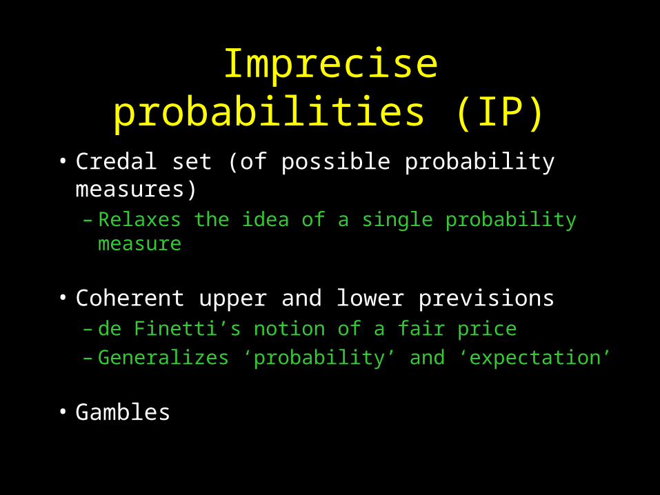
Imprecise probabilities (IP)

• Credal set (of possible probability measures)– Relaxes the idea of a single probability measure

• Coherent upper and lower previsions– de Finetti’s notion of a fair price– Generalizes ‘probability’ and ‘expectation’

• Gambles

Three pillars of IP

• Behavioral definition of probability– Can be operationalized

• Natural extension – Linear programming to compute answers

• Rationality criteria– Avoiding sure losses (Dutch books)– Coherence (logical closure)

Probability of an event

• Imagine a gamble that pays one dollar if an event occurs (but nothing otherwise)– How much would you pay to buy this gamble?– How much would you be willing to sell it for?

• Probability theory requires the same price for both– By asserting the probability of the event, you agree to

buy any such gamble offered for this amount or less, and to sell the same gamble for any amount less than or equal to this ‘fair’ price …and for every event!

• IP just says, sometimes, your highest buying price might be smaller than your lowest selling price

Credal set

• Knowledge and judgments are used to define a set of possible probability measures M

– All distributions within bounds are possible– Only distributions having a given shape

– Probability of an event is within some interval– Event A is at least as probable as event B– Nothing is known about the probability of C

IP generalizes other approaches

• Probability theory• Bayesian analysis• Worst-case analysis, info-gap theory• Possibility / necessity models• Dempster-Shafer theory, belief / plausibility functions• Probability intervals, probability bounds analysis• Lower/upper mass/density functions• Robust Bayes, Bayesian sensitivity analysis• Random set models• Coherent lower previsions

DeFinetti probability measuresCredal setsDistributions with interval-valued parametersContamination modelsChoquet capacities, 2-monotone capacities

Assumptions

• Everyone makes assumptions

• But not all sets of assumptions are equal!Linear Gaussian Independent

Montonic Unimodal Known correlation sign

Any function Any distribution Any dependence

• IP doesn’t require unwarranted assumptions– “Certainties lead to doubt; doubts lead to certainty”

Activities in engineering design

• Decision making• Optimization• Constraint propagation

• Convolutions– Arithmetic– Logic (event trees)

• Updating• Validation• Sensitivity analyses

…sometimes

…often

…a lot

Convolutions

(i.e., adding, multiplying, and-gating, or-gating, etc., for

quantifying the reliability or risk associated with a design)

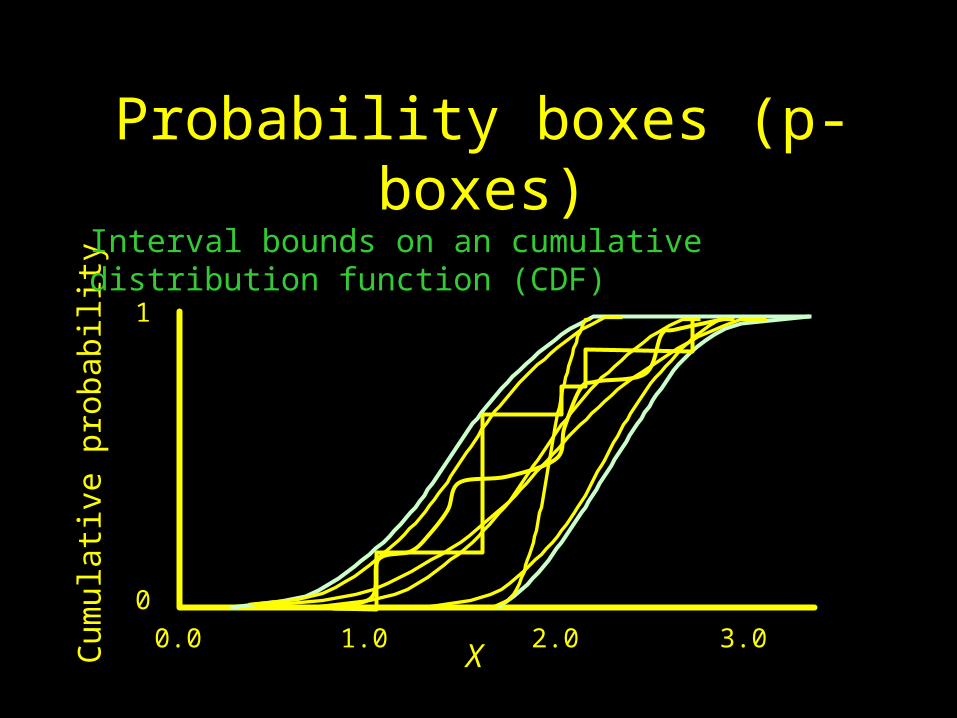
Probability boxes (p-boxes)

0

1

1.0 2.0 3.0 0.0X

Cum

ulat

ive

prob

abil

ity

Interval bounds on an cumulative distribution function (CDF)

A few ways p-boxes ariseC

DF

1

0

min max

Interval

min maxmean

Non-parametric (unknown shape)

Cumulative histogram of interval data Envelope of alternative distributions

Known shape with interval parameters

Precise distribution

P-box arithmetic (and logic)

• All standard mathematical operations– Arithmetic operations (+, , ×, ÷, ^, min, max)– Logical operations (and, or, not, if, etc.)– Transformations (exp, ln, sin, tan, abs, sqrt, etc.)– Other operations (envelope, mixture, etc.)

• Faster than Monte Carlo• Guaranteed to bounds answer• Optimal answers generally require LP

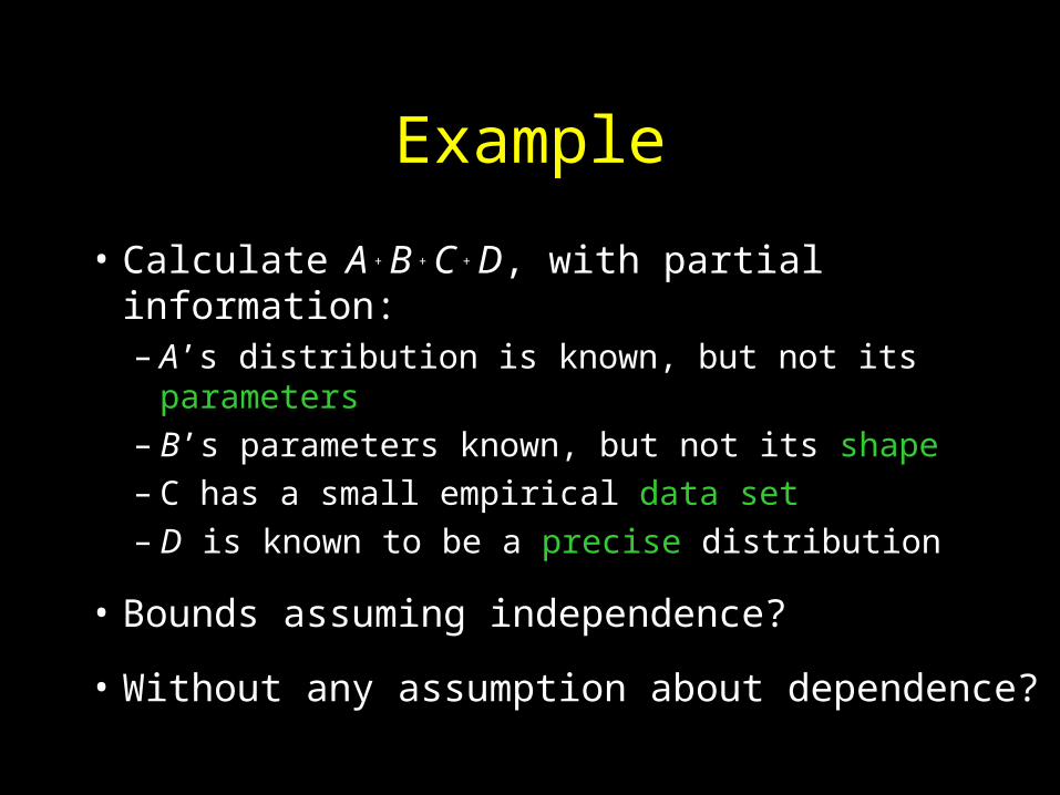
Example

• Calculate A + B + C + D, with partial information:– A’s distribution is known, but not its parameters – B’s parameters known, but not its shape– C has a small empirical data set– D is known to be a precise distribution

• Bounds assuming independence?

• Without any assumption about dependence?

A = {lognormal, mean = [.5,.6], variance = [.001,.01])B = {min = 0, max = 0.5, mode = 0.3}C = {sample data = 0.2, 0.5, 0.6, 0.7, 0.75, 0.8}D = uniform(0, 1)

A

0 0.2 0.4 0.60

1

B

0 10

1

D

0 10

1

C

CD

FC

DF

0 10

1

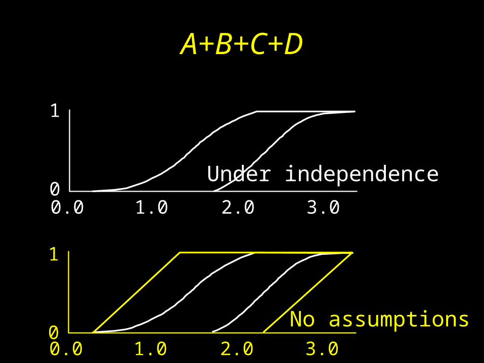
A+B+C+D

No assumptions 1.0 2.0 3.0 0.0

0

1

Under independence 0

1

1.0 2.0 3.0 0.0

Generalization of methods• Marries interval analysis with probability theory

– When information abundant, same as probability theory

– When inputs only ranges, agrees with interval analysis

• Can’t get these answers from Monte Carlo methods

• Fewer assumptions– Not just different assumptions

– Distribution-free methods

• Rigorous results– Automatically verified calculations

– Built-in quality assurance

Can uncertainty swamp the answer?

• Sure, if uncertainty is huge

• This should happen (it’s not “unhelpful”)

• If you think the bounds are too wide, then put in whatever information is missing

• If there isn’t any such information, do you want the results to mislead?

Decision making

Knight’s dichotomy

• Decisions under risk– The probabilities of various outcomes are known– Maximize expected utility– Not good for big unique decisions or when gambler’s ruin is possible

• Decisions under uncertainty– Probabilities of the outcomes are unknown– Several strategies, depending on the analyst

Decisions under uncertainty

• Pareto (some strategy dominates in all scenarios)• Maximin (largest minimum payoff)• Maximax (largest maximum payoff)• Hurwicz (largest average of min and max payoffs)• Minimax regret (smallest of maximum regret)• Bayes-Laplace (maximum expected payoff

assuming scenarios are equiprobable)

Decision making in IP

• State of the world is a random variable, X X• Outcome (reward) of an action depends on X

• We identify an action a with its reward fa : X R

• In principle, we’d like to choose the decision with the largest expected reward, but how do we do this?

• We explore how the decision changes for different probability measures in M, the set of possible ones

Comparing actions a and b

Strictly preferred a > b Ep( fa) > Ep( fb) for all p M

Almost preferred a b Ep( fa) Ep( fb) for all p M

Indifferent a b Ep( fa) = Ep( fb) for all p M

Incomparable a || b Ep( fa) < Ep( fb) and

Eq( fa) > Eq( fb) some p,q M

where Ep( f ) = p(x) f (x), and

M is the set of possible probability distributions

x X

E-admissibility

• Vary p in M and, assuming it is the correct probability measure, see which decision emerges as the one that maximizes expected utility

• The result is the set of all such decisions for all p M

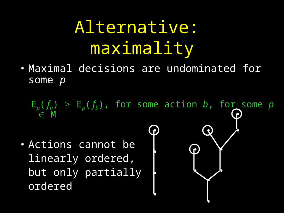
Alternative: maximality

• Maximal decisions are undominated for some p

Ep( fa) Ep( fb), for some action b, for some p M

• Actions cannot be linearly ordered, but only partially ordered

•

• •

•

•

•

•

•

•

•

•

•

•

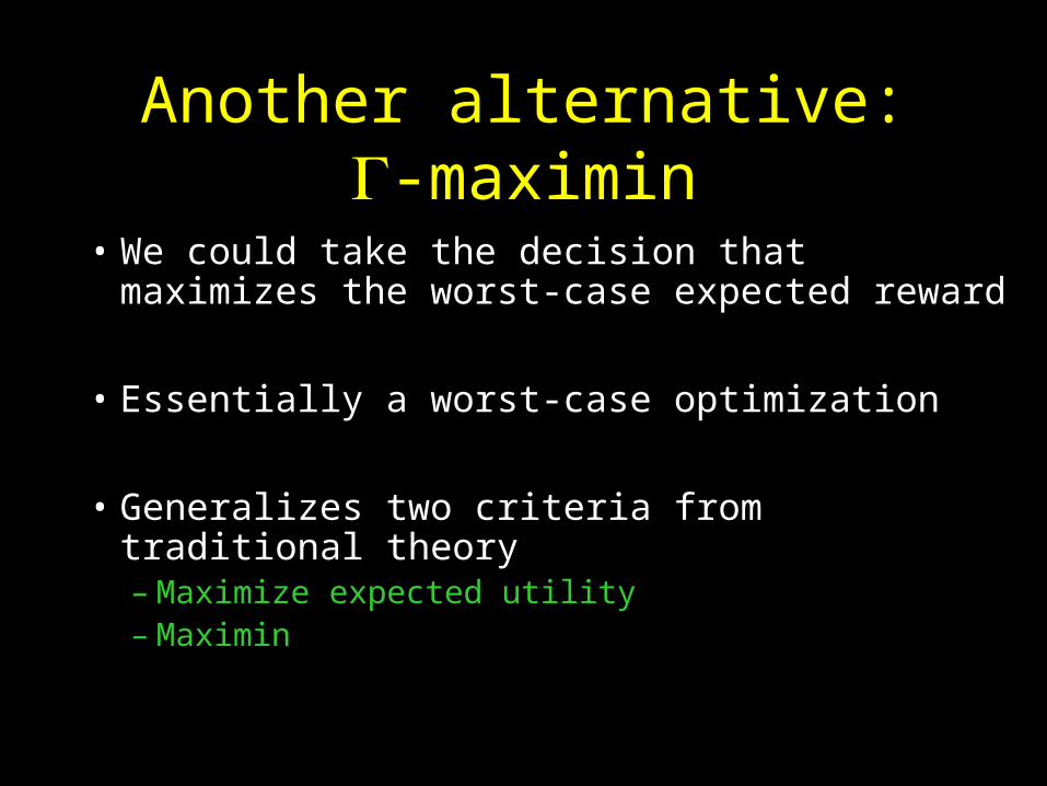
Another alternative: -maximin

• We could take the decision that maximizes the worst-case expected reward

• Essentially a worst-case optimization

• Generalizes two criteria from traditional theory– Maximize expected utility– Maximin

Several IP decision criteria

-maximax

E-admissiblemaximal

-maximin

interval dominance

Example

• Suppose we are betting on a coin toss– Only know probability of heads [0.28, 0.7]– Want to decide among six available gambles

1: Pays 4 for heads, pays 0 for tails2: Pays 0 for heads, pays 4 for tails3: Pays 3 for heads, pays 2 for tails4: Pays ½ for heads, pays 3 for tails5: Pays 2.35 for heads, pays 2.35 for tails6: Pays 4.1 for heads, pays 0.3 for tails

(due to Troffaes 2004)

E-admissibility

M is a one-dimensional space of probability measures

Probability Preference

p(H) < 2/5 2

p(H) = 2/5 2, 3 (indifferent)2/5 < p(H) < 2/3 32/5 < p(H) < 2/3 1, 3 (indifferent)2/3 < p(H) 1

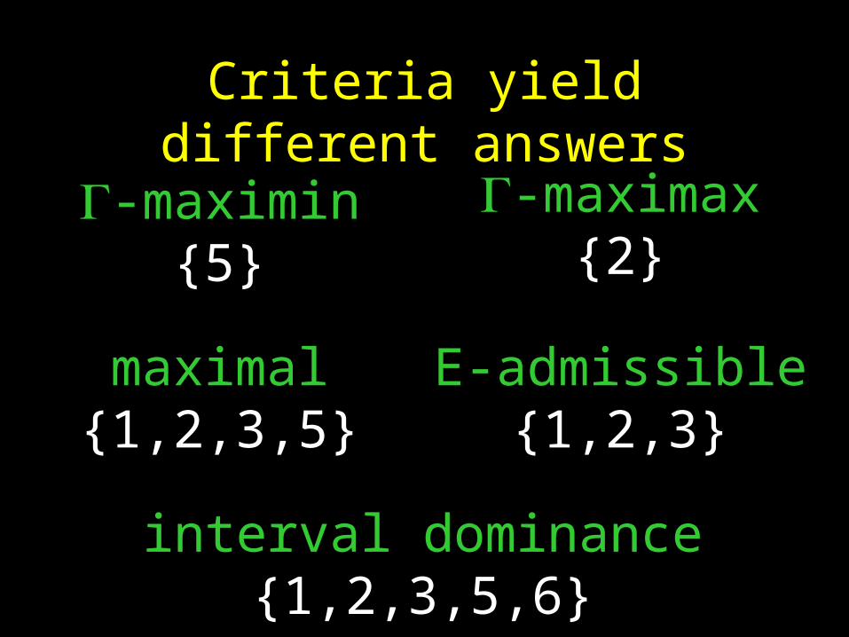
Criteria yield different answers

-maximax{2}

E-admissible{1,2,3}

maximal{1,2,3,5}

-maximin{5}

interval dominance{1,2,3,5,6}

So many answers

• Topic of current discussion and research

• Different criteria are useful in different settings

• The more precise the input, the tighter the outputs

criteria usually yield only one decision

criteria not good if many sequential decisions

• Some argue that E-admissibility is best overall

• Maximality is close to E-admissibility, but much easier to compute, especially for large problems

IP versus traditional approaches

• Decisions under IP allow indecision when your uncertainty entails it

• Bayes always produces a single decision (up to indifference), no matter how little information may be available

• IP unifies the two poles of Knight’s division into a continuum

Comparison to Bayesian approach

• Axioms identical except IP doesn’t use completeness

• Bayesian rationality implies not only avoidance of sure loss & coherence, but also the idea that an agent must agree to buy or sell any bet at one price

• “Uncertainty of probability” is meaningful, and it’s operationalized as the difference between the max buying price and min selling price

• If you know all the probabilities (and utilities) perfectly, then IP reduces to Bayes

Why Bayes fares poorly

• Bayesian approaches don’t distinguish ignorance from equiprobability

• Neuroimaging and clinical psychology shows humans strongly distinguish uncertainty from risk– Most humans regularly and strongly deviate from Bayes– Hsu (2005) reported that people who have brain lesions

associated with the site believed to handle uncertainty behave according to the Bayesian normative rules

• Bayesians are too sure of themselves (e.g., Clippy)

Robust Bayes

Derivation of Bayes’ rule

P(A | B) P(B) = P(A & B) = P(B | A) P(A)

P(A | B) = P(A) P(B | A) / P(B)

The prevalence of a disease in the general population is 0.01%. If a diseased person is tested, there’s a 99.9% chance the test is positive. If a healthy person is tested, there’s a 99.99% chance the test is negative.If you test positive, what’s the chance you have the disease?

A

B

A&B

Almost all doctors say 99% or greater, but the true answer is 50%.

-5 0 5 10 15 20-5 0 5 10 15 20

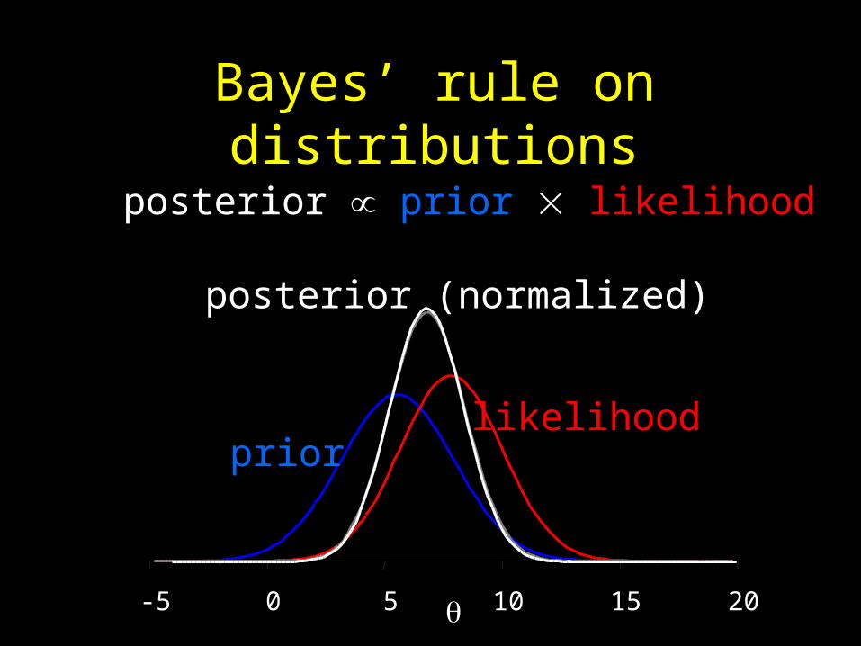
Bayes’ rule on distributions

posterior prior likelihood

-5 0 5 10 15 20

likelihood

posterior (normalized)

prior

Two main problems

• Subjectivity required– Beliefs needed for priors may be inconsistent

with public policy/decision making

• Inadequate model of ignorance– Doesn’t distinguish between ignorance and

equiprobability

Solution: study robustness

• Answer is robust if it doesn’t depend sensitively on the assumptions and inputs

• Robust Bayes analysis, also called Bayesian sensitivity analysis, investigates this

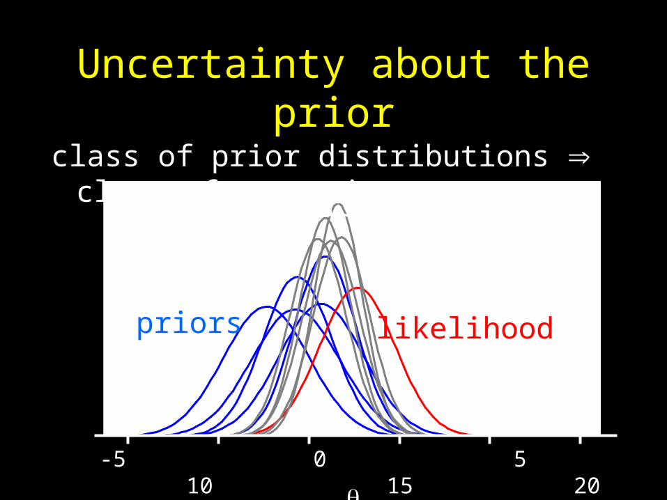
Uncertainty about the prior

class of prior distributions class of posteriors

-5 0 5 10 15 20-5 0 5 10 15 20-5 0 5 10 15 20

likelihood

posteriors

priors

-5 0 5 10 15 20

Uncertainty about the likelihood

-5 0 5 10 15 20-5 0 5 10 15 20-5 0 5 10 15 20

likelihoods

posteriors

prior

class of likelihood functions class of posteriors

-5 0 5 10 15 20

-5 0 5 10 15 20-5 0 5 10 15 20

Uncertainty about both

-5 0 5 10 15 20

Likelihoods

Posteriors

Priors

-5 0 5 10 15 20

Uncertainty about decisions

class of probability models class of decisions

class of utility functions class of decisions

If you end up with a single decision, great.

If the class of decisions is large and diverse, then any conclusion should be rather tentative.

Bayesian dogma of ideal precision

• Robust Bayes is inconsistent with the Bayesian idea that uncertainty should be measured by a single additive probability measure and values should always be measured by a precise utility function.

• Some Bayesians justify it as a convenience

• Others suggest it accounts for uncertainty beyond probability theory

Sensitivity analysis

Sensitivity analysis with p-boxes

• Local sensitivity via derivatives

• Explored macroscopically over the uncertainty in the input

• Describes the ensemble of tangent slopes to the function over the range of uncertainty

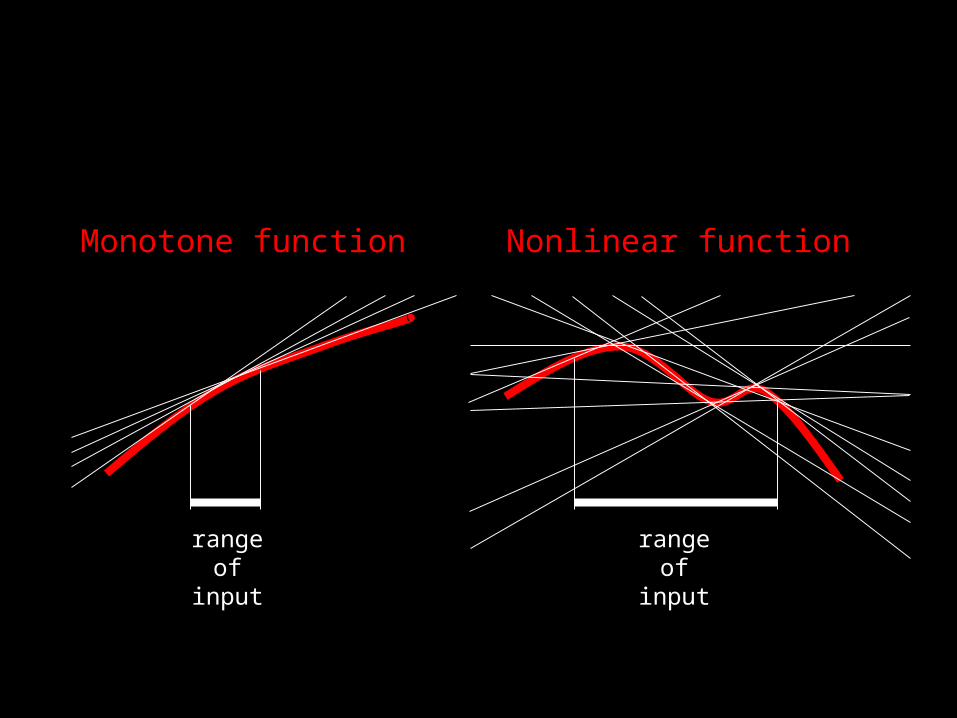
range of input

range of input

Monotone function Nonlinear function

Sensitivity analysis of p-boxes

• Quantifies the reduction in uncertainty of a result when an input is pinched

• Pinching is hypothetically replacing it by a less uncertain characterization

Pinching to a point value

0

1

1 2 30 X

Cum

ulat

ive

prob

abil

ity

0

1

1 2 30 XC

umul

ativ

e pr

obab

ilit

y

Pinching to a (precise) distribution

0

1

1 2 30 X

Cum

ulat

ive

prob

abil

ity

0

1

1 2 30 XC

umul

ativ

e pr

obab

ilit

y

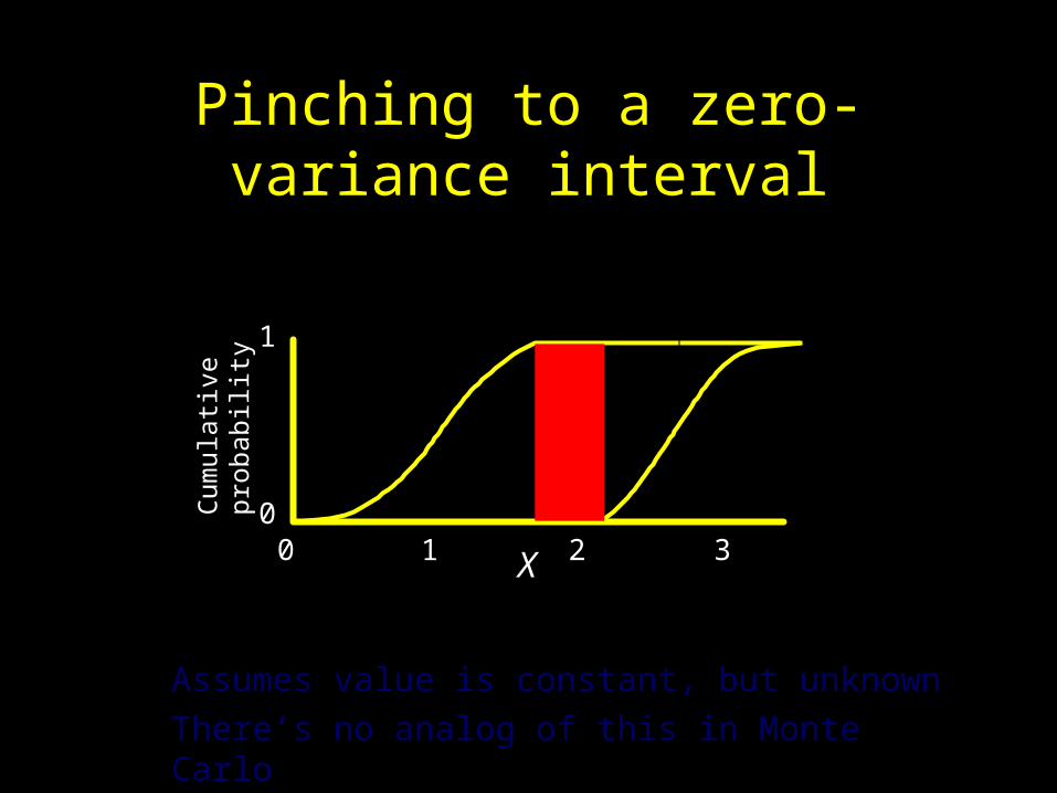
Pinching to a zero-variance interval

Assumes value is constant, but unknown

There’s no analog of this in Monte Carlo

0

1

1 2 30 X

Cum

ulat

ive

prob

abil

ity

Using sensitivity analyses

There is only one take-home message:

“Shortlisting” variables for treatment is bad– Reduces dimensionality, but erases uncertainty

Validation

200

250

300

350

400

1000900800700600

Time [seconds]

Tem

pera

ture

[de

gree

s C

elsi

us]

How the data come

How we look at them

0

1

Pro

babi

lity

200 250 300 350 450400Temperature

0

1

Pro

babi

lity

200 250 300 350 450400Temperature

One suggestion for a metric

Area or average horizontal distance between the empirical distribution Sn and the predicted distribution

Pooling data comparisons

• When data are to be compared against a single distribution, they’re pooled into Sn

• When data are compared against different distributions, this isn’t possible

• Conformance must be expressed on some universal scale

Universal scale

ui=Fi (xi) where xi are the data and Fi are their

respective predictions

1 10 100 10000

1

0 1 2 3 40

1

0 100

1

u1

u2

u3

5

Pro

babi

lity

Pro

babi

lity

Backtransforming to physical scale

u

0 50

1

1 32 4

Pro

babi

lity G

Backtransforming to physical scale

• The distribution of G1(Fi (xi)) represents the

empirical data (like Sn does) but in a common, transformed scale

• Could pick any of many scales, and each leads to a different value for the metric

• The likely distribution of interest is the one used for the validation statement

Epistemic uncertainty in predictions

• In left, the datum evidences no discrepancy at all• In middle, the discrepancy is relative to the edge• In right, the discrepancy is even smaller

Pro

babi

lity

0 10 200

1

0 10 200

1

0 10 200

1

a = N([5,11],1)show a

b = 8.1show b in blue

b = 15

breadth(env(rightside(a),b)) 4.023263478773

b = 11breadth(env(rightside(a),b)) / 2 0.4087173895951 d = 0 d 4 d 0.4

Epistemic uncertainty in bothP

roba

bili

ty

0 5 100

1

0 5 100

1

0 5 100

1

z=0.0001; zz =9.999show z,zza = N([6,7],1)-1show a

b = -1+mix(1,[5,7], 1,[6.5,8], 1,[7.6,9.99], 1, [3.3,6], 1,[4,8], 1,[4.5,8], 1,[5,7], 1,[7.5,9], 1,[4,8], 1,[5,9], 1,[6,9.99])show b in blue

b = -0.2+mix(1, [9,9.6],1, [5.3,6.2], 1,[5.6,6], 1,[7.8,8.4], 1,[5.9,7.8], 1,[8.3,8.7], 1,[5,7], 1,[7.5,8], 1,[7.6,9.99], 1, [3.3,6], 1,[4,8], 1,[4.5,8], 1,[5,7], 1,[8.5,9], 1,[7,8], 1,[7,9], 1,[8,9.99])

breadth(env(rightside(a),b)) 2.137345705795

c = -4b = -0.2+mix(1, [9,9.6],1, [5.3,6.2]+c, 1,[5.6,6]+c, 1,[7.8,8.4], 1,[5.9,7.8], 1,[8.3,8.7], 1,[5,7], 1,[7.5,8], 1,[7.6,9.99], 1, [3.3,6], 1,[4,8], 1,[4.5,8]+c, 1,[5,7]+c, 1,[8.5,9], 1,[7,8], 1,[7,9], 1,[8,9.99])

breadth(env(rightside(a),b)) / 2 1.329372857714

d = 0 d 0.05 d 0.07

Predictions in whiteObservations in blue

Backcalculation

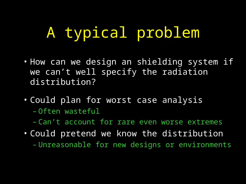
A typical problem

• How can we design an shielding system if we can’t well specify the radiation distribution?

• Could plan for worst case analysis– Often wasteful– Can’t account for rare even worse extremes

• Could pretend we know the distribution– Unreasonable for new designs or environments

IP solution

• Natural compromise that can express both– Gross uncertainty like intervals and worst cases– Distributional information about tail risks

• Need to solve equations containing uncertain numbers– Constraint propagation, or backcalculation

Can’t just invert the equation

Total ionizing dose = Radiation / Shielding

Shielding = Radiation / Dose

When Shielding is put back into the forward equation, the resulting dose is wider than planned

constraints prescribed unknown known

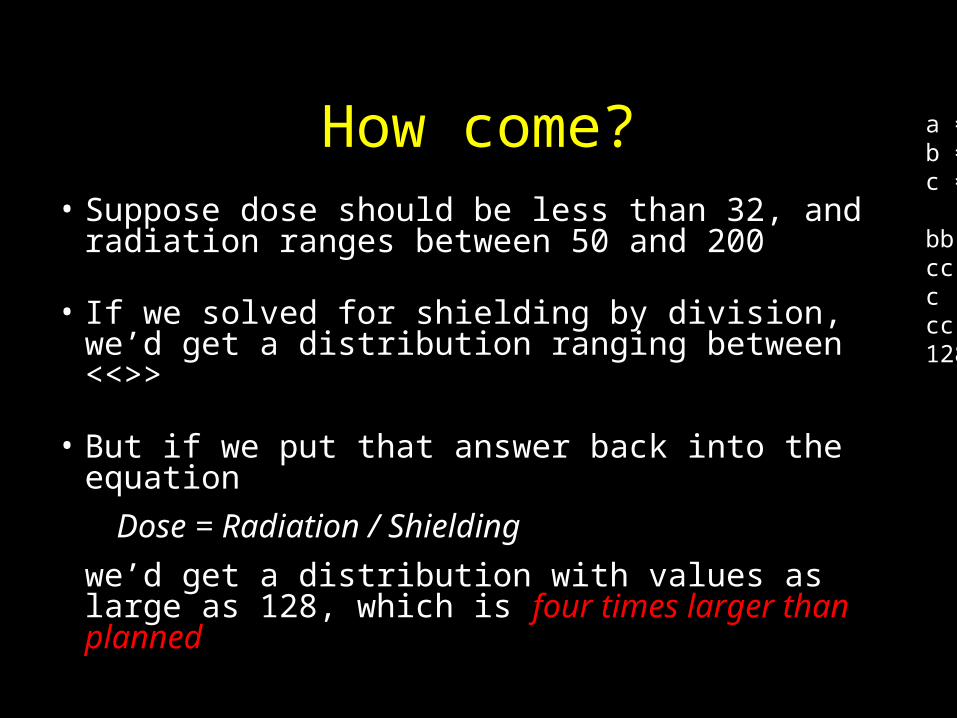
How come?• Suppose dose should be less than 32, and

radiation ranges between 50 and 200

• If we solved for shielding by division, we’d get a distribution ranging between <<>>

• But if we put that answer back into the equation

Dose = Radiation / Shielding

we’d get a distribution with values as large as 128, which is four times larger than planned

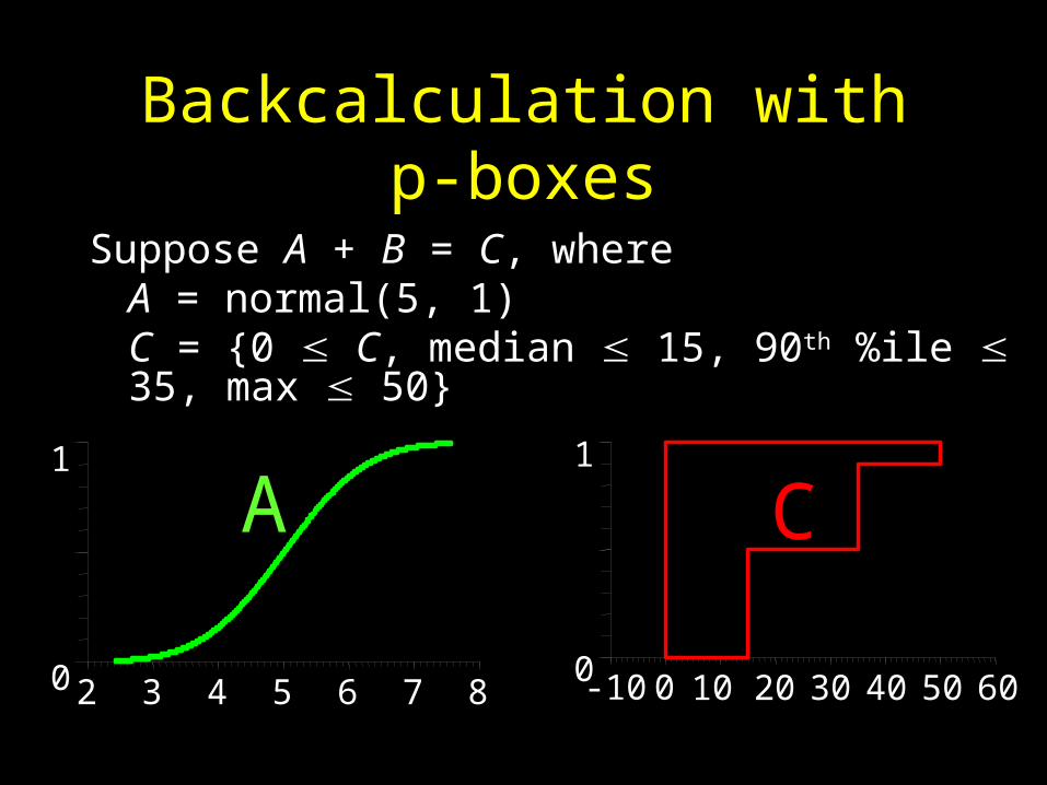
Backcalculation with p-boxes

Suppose A + B = C, where A = normal(5, 1)C = {0 C, median 15, 90th %ile 35, max 50}

2 3 4 5 6 7 80

1

A

-10 0 10 20 30 40 50 600

1

C

Getting the answer

• The backcalculation algorithm basically reverses the forward convolution

• Not hard at all…but a little messy to show

• Any distribution totally inside B is sure to satisfy the constraint … it’s a “kernel”

-10 0 10 20 30 40 500

1

B

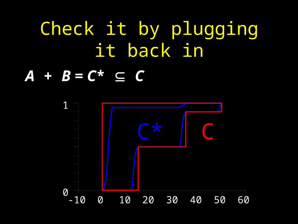
Check it by plugging it back in

A + B = C* C

-10 0 10 20 30 40 50 600

1

C* C

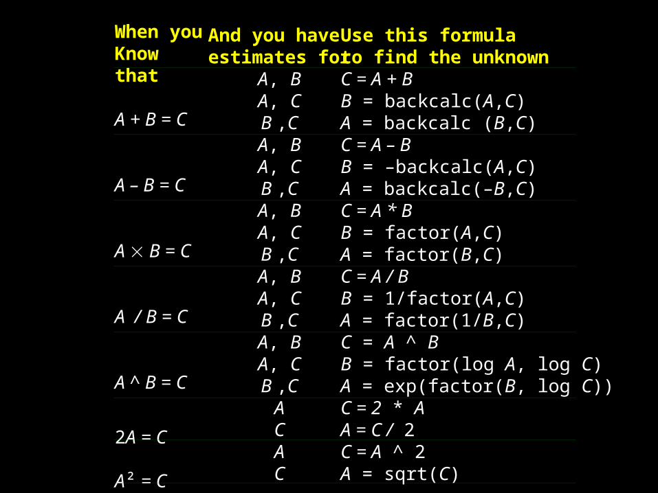
When you Know that

A + B = C

A – B = C

A B = C

A / B = C

A ^ B = C

2A = C

A² = C

And you have estimates for

A, BA, CB ,CA, BA, CB ,CA, BA, CB ,CA, BA, CB ,CA, BA, CB ,C

ACAC

Use this formulato find the unknownC = A + BB = backcalc(A,C)A = backcalc (B,C)C = A – BB = –backcalc(A,C)A = backcalc(–B,C)C = A * BB = factor(A,C)A = factor(B,C)C = A / BB = 1/factor(A,C)A = factor(1/B,C)C = A ^ BB = factor(log A, log C)A = exp(factor(B, log C))C = 2 * AA = C / 2C = A ^ 2A = sqrt(C)

Hard with probability distributions

• Inverting the equation doesn’t work

• Available analytical algorithms are unstable for almost all problems

• Except in a few special cases, Monte Carlo simulation cannot compute backcalculations; trial and error methods are required

Precise distributions don’t work

• Precise distributions can’t express the target

• A specification for shielding giving a prescribed distribution of doses seems to say we want some doses to be high

• Any distribution to the left would be better

• A p-box on the dose target expresses this idea

Conclusions

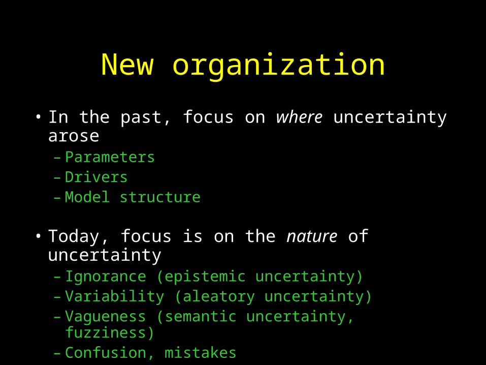
New organization

• In the past, focus on where uncertainty arose– Parameters– Drivers– Model structure

• Today, focus is on the nature of uncertainty– Ignorance (epistemic uncertainty)– Variability (aleatory uncertainty)– Vagueness (semantic uncertainty, fuzziness)– Confusion, mistakes

Untenable assumptions

• Uncertainties are small

• Sources of variation are independent

• Uncertainties cancel each other out

• Linearized models good enough

• Underlying physics is known and modeled

• Computations are inexpensive to make

Need ways to relax assumptions

• Possibly large uncertainties

• Non-independent, or unknown dependencies

• Uncertainties that may not cancel

• Arbitrary mathematical operations

• Model uncertainty

Wishfulthinking

Prudent analysis

Failure

Success

Dumb luck

Negligence Honorable failure

Good engineering

Take-home messages

• It seems antiscientific (or at least silly) to say you know more than you do

• Bayesian decision making always yields one answer, even if this is not really tenable

• IP tells you when you need to be careful and reserve judgment

References

• Cosmides, L., and J. Tooby. 1996. Are humans good intuitive statisticians after All? Rethinking some conclusions from the literature on judgment under uncertainty. Cognition 58:1-73.

• Hsu, M., M. Bhatt, R. Adolphs, D. Tranel, and C.F. Camerer. 2005. Neural systems responding to degrees of uncertainty in human decision-making. Science 310:1680-1683.

• Kmietowicz, Z.W. and A.D. Pearman. 1981. Decision Theory and Incomplete Knowledge. Gower, Hampshire, England.

• Knight, F.H. 1921. Risk, Uncertainty and Profit. L.S.E., London.

• Troffaes, M. 2004. Decision making with imprecise probabilities: a short review. The SIPTA Newsletter 2(1): 4-7.

• Walley, P. 1991. Statistical Reasoning with Imprecise Probabilities. Chapman and Hall, London.

http://www.sciencemag.org/cgi/content/short/310/5754/1680

http://www.sciencedirect.com/science?_ob=ArticleURL&_udi=B6T24-3VXBPWR-1&_user=10&_handle=V-WA-A-W-V-MsSWYWW-UUA-U-AABDWWZUBV-AABVYUZYBV-CVUEBVVZZ-V-U&_fmt=summary&_coverDate=01%2F31%2F1996&_rdoc=1&_orig=browse&_srch=%23toc%234908%231996%23999419998%2370272%21&_cdi=4908&view=c&_acct=C000050221&_version=1&_urlVersion=0&_userid=10&md5=c6985daf53c5402c195c1106cec9622f

Web-accessible reading

http://maths.dur.ac.uk/~dma31jm/durham-intro.pdf(Gert de Cooman’s gentle introduction to imprecise probabilities)

http://www.cs.cmu.edu/~qbayes/Tutorial/quasi-bayesian.html(Fabio’s Cozman’s introduction to imprecise probabilities)

http://idsia.ch/~zaffalon/events/school2004/school.htm(summer school on imprecise probabilities)

http://www.sandia.gov/epistemic/Reports/SAND2002-4015.pdf(introduction to p-boxes and related structures)

http://www.ramas.com/depend.zip(handling dependencies in uncertainty modeling)

http://www.ramas.com/bayes.pdf(introduction to Bayesian and robust Bayesian methods in risk analysis)

http://www.ramas.com/intstats.pdf(statistics for data that may contain interval uncertainty)

End