Implied Volatility Calculations:Hazards of Exotics;Instability for Vanilla Options;Hazards of Newton-Raphson;Solving Non-linear equations

0. WarningI have been expressing these views for several years now and I still do not think the mathematical finance community yet fully appreciates the general foolishness of using implied parameters. Rebonato said that implied volatility was the wrong number to put into the wrong model to get the right answer. This is just the start of the problems, as we shall now see.

In all of the following discussion the so-called implied volatility is "the" solution for s of an equation of the form

(1)PM ‡ VHs, S, K, r, q, tL

where it is assumed that the known market price of a contract is PM and all the parameters S, K, r, q, t, … of a model value V are all known with certainty.

Off@General::spell1D;Off@FindRoot::lstolD;

Now we have some simple models (analytical and finite-difference) for pricing vanilla instruments, we need to take a look at this calcula-tion. Then we shall return to a numerical discussion to treat "American" calculations. But today we shall try to probe the very real issues that arise in solving a non-linear equation, and the astonishing complications that can arise. We shall even have an excuse to draw some fractals.

1. IntroductionThe journals and magazines that deal with derivatives are fascinated by volatility modelling. Models of extraordinary detail are now being built to explain observed volatility skews and smiles. These include 2+-factor models, GARCH models and their relatives, as well as older elasticity-type models of the type you have been asked to look at in your project.

Such exotic structures need to be built on firm foundations. This note explores the foundations, which to my mind consist at present of a house of cards built on quicksand. Why do I say this? One of our primary goals is to understand and exploit the way volatility data is implied by market pricing information. The construction of a volatility surface, and/or its cross-sections in the form of skews or smiles, is fundamental to this process. This requires that the computation of volatility surfaces from pricing data is a "meaningful" process. The problem is that the inversion of option-pricing formulae is, depending on parameters, potentially a highly unstable process. When the inversion is unstable, a tiny change in a market price can cause a huge change in the "implied volatility". Any noise in the price or in the valuation algorithm can be reflected in massive shifts in volatility, so that the volatility that is calculated is essentially meaningless. "Noise" in the price can arise from, for example,

(i) bid-offer spread;

(ii) post-theory price adjustments based on psychology;

(iii) tick-size (price quantization) effects,

and any error in the valuation algorithm will also produce noise that may amplified in the volatility computation. This lecture gets a grip on when market data is actually un-usable for calculating a vol surface.

But first, In order to bring home some of the dangers, I will begin this analysis by taking a look at some simpler options than vanilla Calls and Puts, where there is a closed-form analytic solution for the implied volatility. Two interesting examples are the log and power contract, which I discussed in Chapter 5 of MFDwM, and which exhibit the phenomena of instability and non-existence of the implied volatility. The instrument that is closest to the vanilla case, and where a closed-form solution is still possible, is the case of European Binary options. I appreciate that these may not necessarily be routinely used for defining volatility, but they are a very valuable exercise for getting one out of the rather unfortunate, and completely erroneous, state of mind that the extraction of implied volatilities is a breeze! This is a particularly amusing case as the issues can be explored using only the elementary theory of quadratic equations.

Then we shall explore the most important case of vanilla European call or put options that are in-the-money and/or short-dated (matters are worse when both apply). As one goes deeper in the money, or approach maturity, the implied volatility becomes so unstable as to be meaningless. An example is given to show how even a tiny uncertainty in spread implicit in the market price can induce a fake skew in the computed volatility surface. Any flat charge in the quoted price will induce a smile just as easily.

Fake structure in the volatility surface can be created in other ways, including disagreement between market participants about interest rates, yields and times to maturity induced by inconsistent calendar tool. In the case of equities there is the fundamental issue of not really knowing the future dividends.

All of these problems are associated with the failure, or near failure, of the inverse function theorem.

Finally we look at another case that is "in the neighbourhood" of the vanilla instrument but different in another way - the case of the Convertible Bond. Here the presence of further uncertain parameters introduces additional uncertainty into the implied volatility. Similar issues arise from not really knowing the future dividends.

Equation-Solving in other Finance ApplicationsThe calculation of implied volatility is not the only place where one might wish to solve a non-linear equation to find some parameter of interest, though it is (IMHO) the most notorious. Some other examples include:

‡ Solving a dividend-discount model

There are several valuation/comparison models based on the concept that the price of an asset is the present value of its future cash flows. For example, if an equity with market price P has a future dividend stream Di, for simplicity one a year starting one year hence, we define the internal rate of return to be the solution of the equation 2

P ‡‚i=1

M

H1 + rL-i Di

‡ Finding a Quantile

In general Monte Carlo simulation, if you know the CDF FHxL associated with a density f HxL then given a sample U from a uniform distribution a sample from the given distribution is given by

X = F-1HUL

where F-1denotes the functional inverse.This inverse function is called the Quantile Function and is defined by the integral equation

u ‡ ‡-¶

xf HyL „ y

Solution of this for x given u gives the Quantile Function. It is particularly useful to know it if you are working with copulas, where simulation of the copula gives you samples from a unit hypercube. Then the QF takes to the relevant sample point. This separates the simulation of dependency from the simulation of the marginals. (See my papers page for two recent papers on the T distribution, where the QF calculation can be reduced to solution of a polynomial in certain cases.)

2. A Perverse Case - Binary OptionsIt is a revealing exercise to pursue the question of "implied volatility" for simple European binary options, for in this case the calculation (including the instability and multi-valuedness) is analytically tractable using only the simple theory of quadratic equations. (No Newton-Raphson or bisection solvers are needed).

The value of a European Binary Call option, paying out cash B if the underlying S is greater than K at maturity, is

CB = B ‰-r t F Hd2L

and that for a Put (B paid if S < K) is

PB = B ‰-r t FH- d2L

where, F is the cumulative normal distribution function, d2 is the usual thing, which we write in the form

d2 =a

s t-s t

2

and where

a = logS ‰-q t

K ‰-r t

You might find it useful to make some simple modifications to the C++ code for vanilla instruments to price this instrument. In writing the model in this way we are thinking primarily of either equity indices or FX, where the q-picture of dividends/foreign FX rates is most appropriate.

Now suppose we are given market prices CM or PM for such instruments. Provided, in each case

0 < CM < B ‰-r t

0 < PM < B ‰-r t

the pricing formula can be partially inverted to find d2 as a function of market price. We just have, respectively

d2 = F-1 HCM ‰r t êBL

and, for a Put:

d2 = -F-1 HPM ‰r t êBL

A Mathematica implementation of the inverse cumulative distribution function is:

3

A Mathematica implementation of the inverse cumulative distribution function is:

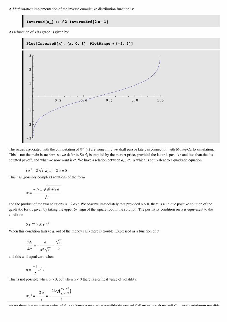
InverseN@x_D := 2 InverseErf@2 x - 1D

As a function of x its graph is given by:

Plot@InverseN@xD, 8x, 0, 1<, PlotRange Ø 8-3, 3<D

0.2 0.4 0.6 0.8 1.0

-3

-2

-1

1

2

3

The issues associated with the computation of F-1HxL are something we shall pursue later, in connection with Monte-Carlo simulation. This is not the main issue here, so we defer it. So d2 is implied by the market price, provided the latter is positive and less than the dis-counted payoff, and what we now want is s. We have a relation between d2, s, a which is equivalent to a quadratic equation:

t s2 + 2 t d2 s - 2 a = 0

This has (possibly complex) solutions of the form

s =-d2 ± d22 + 2 a

t

and the product of the two solutions is -2 a ê t. We observe immediately that provided a > 0, there is a unique positive solution of the quadratic for s, given by taking the upper (+) sign of the square root in the solution. The positivity condition on a is equivalent to the condition

S ‰-q t > K ‰-r t

When this condition fails (e.g. out of the money call) there is trouble. Expressed as a function of s

¶∂d2¶∂s

= -a

s2 t-

t

2

and this will equal zero when

a =-1

2s2 t

This is not possible when a > 0, but when a < 0 there is a critical value of volatility:

sC2 = -

2 a

t= -

2 logJ S ‰-q t

K ‰-r tN

t

where there is a maximum value of d2, and hence a maximum possible theoretical Call price, which we call Ccrit, and a minimum possible theoretical Put price, Pcrit. We proceed further for the case of a Call - the Put goes through similarly.

If in the case a < 0 the market call price exceeds that given by sc, there is no implied volatility consistent with the given market price. If it is less than this critical value, there are two implied volatilities.

So in total there are three cases for a Call provided 0 < CM < B ‰-r t:

(i) a > 0: a unique real and positive implied volatility;

(ii) a < 0 and CM > Ccrit: no implied volatility;

(iii) a < 0 and CM < Ccrit: two implied volatilitities.

4

where there is a maximum value of d2, and hence a maximum possible theoretical Call price, which we call Ccrit, and a minimum possible theoretical Put price, Pcrit. We proceed further for the case of a Call - the Put goes through similarly.

If in the case a < 0 the market call price exceeds that given by sc, there is no implied volatility consistent with the given market price. If it is less than this critical value, there are two implied volatilities.

So in total there are three cases for a Call provided 0 < CM < B ‰-r t:

(i) a > 0: a unique real and positive implied volatility;

(ii) a < 0 and CM > Ccrit: no implied volatility;

(iii) a < 0 and CM < Ccrit: two implied volatilitities.

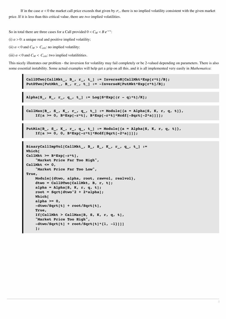
This nicely illustrates our problem - the inversion for volatility may fail completely or be 2-valued depending on parameters. There is also some essential instability. Some actual examples will help get a grip on all this, and it is all implemented very easily in Mathematica:

CallDTwo[CallMkt_, B_, r_, t_] := InverseN[CallMkt*Exp[r*t]/B]; PutDTwo[PutMkt_, B_, r_, t_] := -InverseN[PutMkt*Exp[r*t]/B];

Alpha[S_, K_, r_, q_, t_] := Log[S*Exp[(r - q)*t]/K];

CallMax[B_, S_, K_, r_, q_, t_] := Module[{a = Alpha[S, K, r, q, t]}, If[a >= 0, B*Exp[-r*t], B*Exp[-r*t]*Ncdf[-Sqrt[-2*a]]]];

PutMin[B_, S_, K_, r_, q_, t_] := Module[{a = Alpha[S, K, r, q, t]}, If[a >= 0, 0, B*Exp[-r*t]*Ncdf[Sqrt[-2*a]]]];

BinaryCallImpVol[CallMkt_, B_, S_, K_, r_, q_, t_] := Which[CallMkt >= B*Exp[-r*t], "Market Price Far Too High", CallMkt <= 0, "Market Price Far Too Low", True,

Module[{dtwo, alpha, root, rawvol, realvol}, dtwo = CallDTwo[CallMkt, B, r, t]; alpha = Alpha[S, K, r, q, t]; root = Sqrt[dtwo^2 + 2*alpha]; Which[alpha >= 0, -dtwo/Sqrt[t] + root/Sqrt[t], True, If[CallMkt > CallMax[B, S, K, r, q, t], "Market Price Too High", -dtwo/Sqrt[t] + root/Sqrt[t]*{1, -1}]]]];

5

BinaryPutImpVol[PutMkt_, B_, S_, K_, r_, q_, t_] := Which[PutMkt >= B*Exp[-r*t], "Market Price Far Too High", PutMkt <= 0, "Market Price Far Too Low", True, Module[{dtwo, alpha, root, rawvol, realvol}, dtwo = PutDTwo[PutMkt, B, r, t]; alpha = Alpha[S, K, r, q, t]; root = Sqrt[dtwo^2 + 2*alpha]; Which[ alpha >= 0, -dtwo/Sqrt[t] + root/Sqrt[t], True, If[PutMkt < PutMin[B, S, K, r, q, t], "Market Price Too Low", -dtwo/Sqrt[t] + root/Sqrt[t]*{1, -1}]]] ];

Here are some examples with a Call:

BinaryCallImpVol@10, 10, 100, 100, 0.05, 0, 1D

Market Price Far Too High

BinaryCallImpVol@5, 10, 100, 100, 0.05, 0, 1D

0.258396

Going further in the money is fine:

BinaryCallImpVol@5, 10, 105, 100, 0.05, 0, 1D

0.384824

When we come out of the money a superficially reasonable market price is has no matching implied vol within the model:

BinaryCallImpVol@4, 10, 90, 100, 0.05, 0, 1D

Market Price Too High

Lowering the market price slightly produces two answers - which of the following implied vols is the "right" one?

BinaryCallImpVol@3.5, 10, 90, 100, 0.05, 0, 1D

80.392539, 0.282064<

If you do not believe this makes sense, try calculating and plotting the call value as a function of s with these parameters, using the following code lifted from Chapter 6 of [MFDwM]:

Ncdf@x_D := H1 + Erf@x ê Sqrt@2DDL ê 2;

dtwo@s_, v_, k_, t_, r_, q_D :=HHr - qL * t + Log@s ê kDL ê Hv * Sqrt@tDL - Hv * Sqrt@tDL ê 2;

BinaryCall@B_, S_, K_, v_, r_, q_, t_D := B * Exp@-r * tD * Ncdf@dtwo@S, v, K, t, r, qDD;6

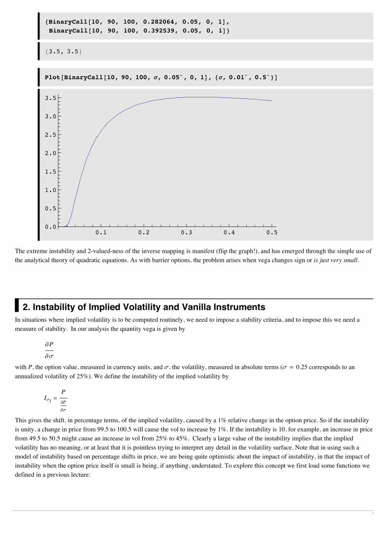
8BinaryCall@10, 90, 100, 0.282064, 0.05, 0, 1D,BinaryCall@10, 90, 100, 0.392539, 0.05, 0, 1D<

83.5, 3.5<

Plot@BinaryCall@10, 90, 100, s, 0.05`, 0, 1D, 8s, 0.01`, 0.5`<D

0.1 0.2 0.3 0.4 0.50.0

0.5

1.0

1.5

2.0

2.5

3.0

3.5

The extreme instability and 2-valued-ness of the inverse mapping is manifest (flip the graph!), and has emerged through the simple use of the analytical theory of quadratic equations. As with barrier options, the problem arises when vega changes sign or is just very small.

2. Instability of Implied Volatility and Vanilla InstrumentsIn situations where implied volatility is to be computed routinely, we need to impose a stability criteria, and to impose this we need a measure of stability. In our analysis the quantity vega is given by

¶∂P

¶∂s

with P, the option value, measured in currency units, and s, the volatility, measured in absolute terms (s = 0.25 corresponds to an annualized volatility of 25%). We define the instability of the implied volatility by

IsI =P¶∂P¶∂s

This gives the shift, in percentage terms, of the implied volatility, caused by a 1% relative change in the option price. So if the instability is unity, a change in price from 99.5 to 100.5 will cause the vol to increase by 1%. If the instability is 10, for example, an increase in price from 49.5 to 50.5 might cause an increase in vol from 25% to 45%. Clearly a large value of the instability implies that the implied volatility has no meaning, or at least that it is pointless trying to interpret any detail in the volatility surface. Note that in using such a model of instability based on percentage shifts in price, we are being quite optimistic about the impact of instability, in that the impact of instability when the option price itself is small is being, if anything, understated. To explore this concept we first load some functions we defined in a previous lecture:

7

done[s_, s_, k_, t_, r_, q_] := ((r - q)*t + Log[s/k])/(s*Sqrt[t]) + (s*Sqrt[t])/2;

BlackScholesCall[s_, k_, s_, r_, q_, t_] := s*Exp[-q*t]*Ncdf[done[s, s, k, t, r, q]] - k*Exp[-r*t]*Ncdf[dtwo[s, s, k, t, r, q]];

BlackScholesCallVega[s_,k_, v_, r_, q_, t_]= Evaluate[D[BlackScholesCall[s,k, v, r, q, t], v]];

CallIVInstability@S_, K_, s_, r_, q_, t_D :=BlackScholesCall@S, K, s, r, q, tD ê BlackScholesCallVega@S, K, s, r, q, tD

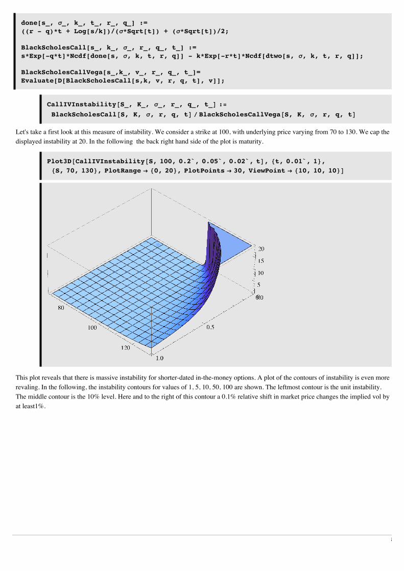
Let's take a first look at this measure of instability. We consider a strike at 100, with underlying price varying from 70 to 130. We cap the displayed instability at 20. In the following the back right hand side of the plot is maturity.

Plot3D@CallIVInstability@S, 100, 0.2`, 0.05`, 0.02`, tD, 8t, 0.01`, 1<,8S, 70, 130<, PlotRange Ø 80, 20<, PlotPoints Ø 30, ViewPoint Ø 810, 10, 10<D

This plot reveals that there is massive instability for shorter-dated in-the-money options. A plot of the contours of instability is even more revaling. In the following, the instability contours for values of 1, 5, 10, 50, 100 are shown. The leftmost contour is the unit instability. The middle contour is the 10% level. Here and to the right of this contour a 0.1% relative shift in market price changes the implied vol by at least1%.

8

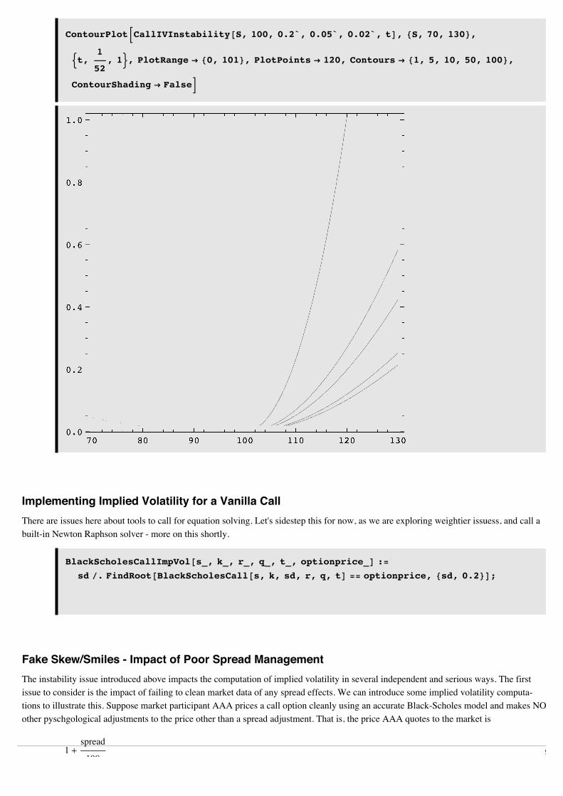
ContourPlotBCallIVInstability@S, 100, 0.2`, 0.05`, 0.02`, tD, 8S, 70, 130<,

:t,1

52, 1>, PlotRange Ø 80, 101<, PlotPoints Ø 120, Contours Ø 81, 5, 10, 50, 100<,

ContourShading Ø FalseF

Implementing Implied Volatility for a Vanilla CallThere are issues here about tools to call for equation solving. Let's sidestep this for now, as we are exploring weightier issuess, and call a built-in Newton Raphson solver - more on this shortly.

BlackScholesCallImpVol@s_, k_, r_, q_, t_, optionprice_D :=sd ê. FindRoot@BlackScholesCall@s, k, sd, r, q, tD == optionprice, 8sd, 0.2<D;

Fake Skew/Smiles - Impact of Poor Spread ManagementThe instability issue introduced above impacts the computation of implied volatility in several independent and serious ways. The first issue to consider is the impact of failing to clean market data of any spread effects. We can introduce some implied volatility computa-tions to illustrate this. Suppose market participant AAA prices a call option cleanly using an accurate Black-Scholes model and makes NO other pyschgological adjustments to the price other than a spread adjustment. That is, the price AAA quotes to the market is

1 +spread

100

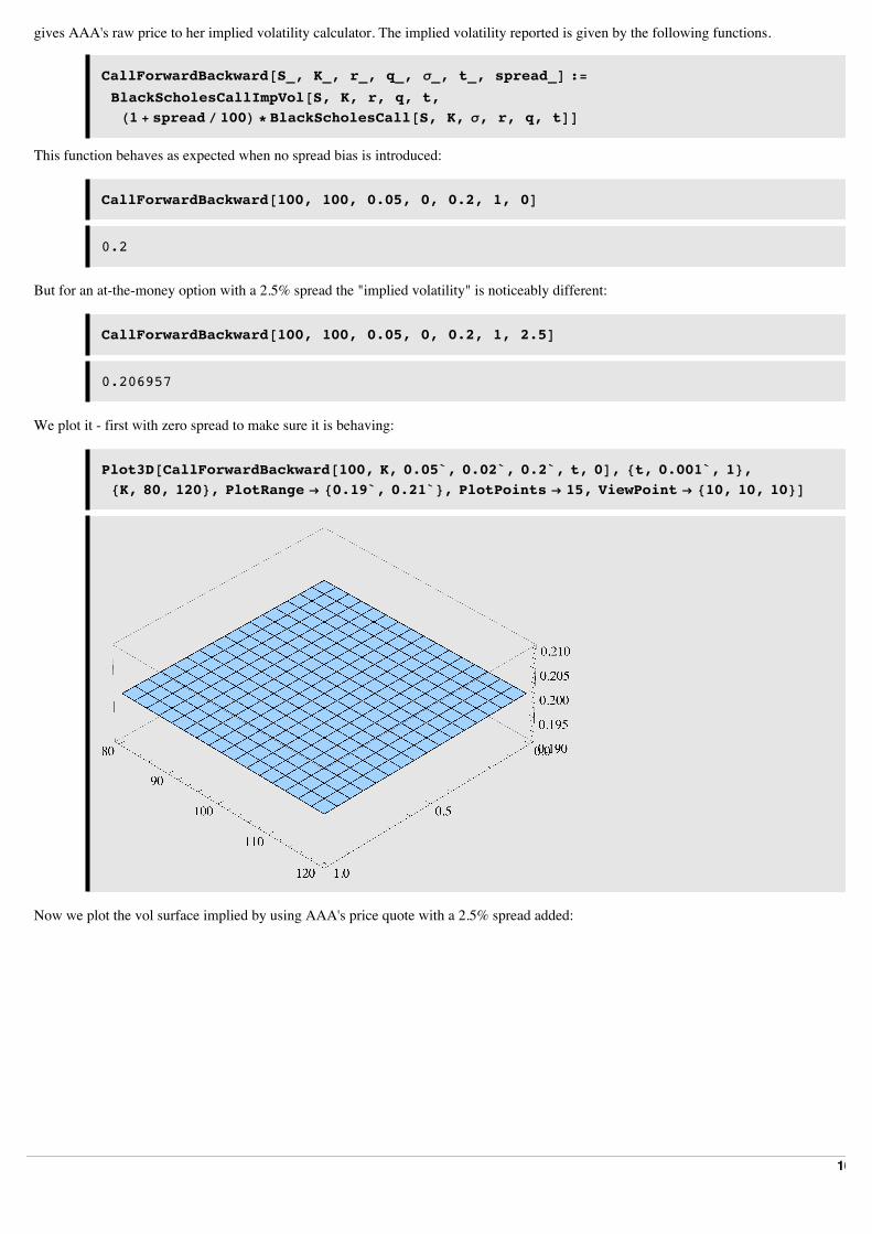
times the clean Black-Scholes value with a given fixed volatility. Participant BBB is equipped with an accurate Black-Scholes model and gives AAA's raw price to her implied volatility calculator. The implied volatility reported is given by the following functions.

9

times the clean Black-Scholes value with a given fixed volatility. Participant BBB is equipped with an accurate Black-Scholes model and gives AAA's raw price to her implied volatility calculator. The implied volatility reported is given by the following functions.

CallForwardBackward@S_, K_, r_, q_, s_, t_, spread_D :=BlackScholesCallImpVol@S, K, r, q, t,H1 + spread ê 100L * BlackScholesCall@S, K, s, r, q, tDD

This function behaves as expected when no spread bias is introduced:

CallForwardBackward@100, 100, 0.05, 0, 0.2, 1, 0D

0.2

But for an at-the-money option with a 2.5% spread the "implied volatility" is noticeably different:

CallForwardBackward@100, 100, 0.05, 0, 0.2, 1, 2.5D

0.206957

We plot it - first with zero spread to make sure it is behaving:

Plot3D@CallForwardBackward@100, K, 0.05`, 0.02`, 0.2`, t, 0D, 8t, 0.001`, 1<,8K, 80, 120<, PlotRange Ø 80.19`, 0.21`<, PlotPoints Ø 15, ViewPoint Ø 810, 10, 10<D

Now we plot the vol surface implied by using AAA's price quote with a 2.5% spread added:

10

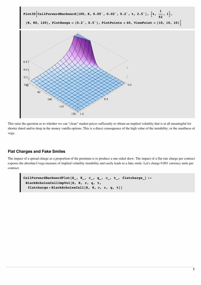
Plot3DBCallForwardBackward@100, K, 0.05`, 0.02`, 0.2`, t, 2.5`D, :t,1

52, 1>,

8K, 80, 120<, PlotRange Ø 80.2`, 0.5`<, PlotPoints Ø 40, ViewPoint Ø 810, 10, 10<F

This raise the question as to whether we can "clean" market prices sufficently to obtain an implied volatility that is at all meaningful for shorter dated and/or deep in the money vanilla options. This is a direct consequence of the high value of the instability, or the smallness of vega.

Flat Charges and Fake SmilesThe impact of a spread charge as a proportion of the permium is to produce a one-sided skew. The impact of a flat rate charge per contract exposes the absolute1/vega measure of implied volatility instability and easily leads to a fake smile. Let's charge 0.001 currency units per contract.

CallForwardBackwardFlat@S_, K_, r_, q_, s_, t_, flatcharge_D :=BlackScholesCallImpVol@S, K, r, q, t,flatcharge + BlackScholesCall@S, K, s, r, q, tDD

11

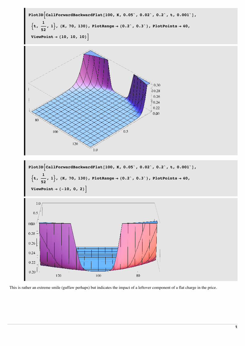
Plot3DBCallForwardBackwardFlat@100, K, 0.05`, 0.02`, 0.2`, t, 0.001`D,

:t,1

52, 1>, 8K, 70, 130<, PlotRange Ø 80.2`, 0.3`<, PlotPoints Ø 40,

ViewPoint Ø 810, 10, 10<F

Plot3DBCallForwardBackwardFlat@100, K, 0.05`, 0.02`, 0.2`, t, 0.001`D,

:t,1

52, 1>, 8K, 70, 130<, PlotRange Ø 80.2`, 0.3`<, PlotPoints Ø 40,

ViewPoint Ø 8-10, 0, 2<F

This is rather an extreme smile (guffaw perhaps) but indicates the impact of a leftover component of a flat charge in the price.

12

4. Simple Convertible BondsIn the case of convertible bonds, which may contain a complex set of embedded features including Bermudan convertibility, scheduled calls, puts, and refixes, there is considerable scope for instability of the type we have already discussed. For example, in the simplest imaginable type of CB with an underlying paying no dividends and one cash payment at maturity, the value of the CB is the discounted maturity payment plus the value of an option that is effectively European, and hence this CB just inherits the vanilla instability already discussed. The presence of additional option-like features just adds to the mayhem!

But there is an additional complication for this type of instrument, which appears even in the case of the simple Cash+Call picture. In general, for CBs associated with non-government stocks and shares, there are additional uncertain parameters associated with the default risk of the company or instrument. If we simplify (but appreciate that the issue is one of principle, not limited to this simplified picture), and fold the combination of default risk and effective default payoff into a single parameter - the spread, sp, to be applied to discounted cash flows - we view the theoretical price of a CB as a function, other parameters assumed known, of two significant variables:

P = PHs, spL

The precise form of this function is a research-level problem, even for a simple CB. One can consider numerous approaches to determine it, such as,

(i) simple risky bond plus a Call;

(ii) as (i), but lowering the effective spread for higher values of the underlying;

(iii) 2-factor approach, with stochastic processes for both the default and the underlying;

(iv) amalgamation of (iii) to one involving just the value of the firm as underlying.

Whatever route is taken, in remains the case that there are at least two uncertain parameters - three if we treat the default risk and payout-on-default as separate. The issue that arises is then very simple - we cannot estimate s from the market price unless the spread is known with high (very high, for unstable cases) accuracy. In reality, this is seldom possible. One can argue that the spread (or at least the market's view on it) can be estimated from other non-convertible bonds issued by the same company, but these estimates may not be mutually consistent, or may only be available for maturity time-scales different from the CB. Sometimes there may be no such non-convertible bonds available for analysis. Furthermore, although the default of a company is a common influence on all the derivatives associated with it, there might be different effective payouts on default, so that the spread is instrument-specific in an essential way.

What all this boils down to is that given a value for PHs, spL, it is often difficult to assign a value to sp with any reliability. Therefore you cannot estimate an implied value for s. We can say this in other ways, from the mathematical to the obvious. You cannot infer the value of one indepedent variable from a single value of a function of two. You cannot unambiguously calculate the price of oranges from the cost of a bag containing both apples and oranges. What we can do, with a theoretical model, is supply vol-spread contours consistent with the observed market price. Some knowledge about spread may limit us to a portion of this contour. The notion of a vol-spread contour is easily given concrete form if we assume a spread-adjusted theoretical model. For illustration we shall take approach (i) in the list above, though we must point out that what contours emerge are rather sensitive to the model choice (of course this just adds to the uncertainty in the IV). So suppose that our ultra-simple CB, based on a zero-dividend underlying, pays out Z currency units at maturity t, and that there are n shares per bond. Let the price of a European call option on a non-dividend paying stock with current value S, struck at K, volatility s, maturing at t, be the standard Black-Scholes function, which we abbreviate as

CHS,K,s,r,tL

Then the CB value within this simple model (i) is

P = n C S,Z

n, s, r, t + Z ‰-Hr+spL t

In an approach of type (ii), the value of sp might, for example, be lowered from its pure risky-bond value for small S, to zero when S is much higher than Z/n. We can make a trivial reorganization of this equation to have both sides just involving the option component: 13

1

nIP - Z ‰-Hr+spL tM = C S,

Z

n, s, r, t

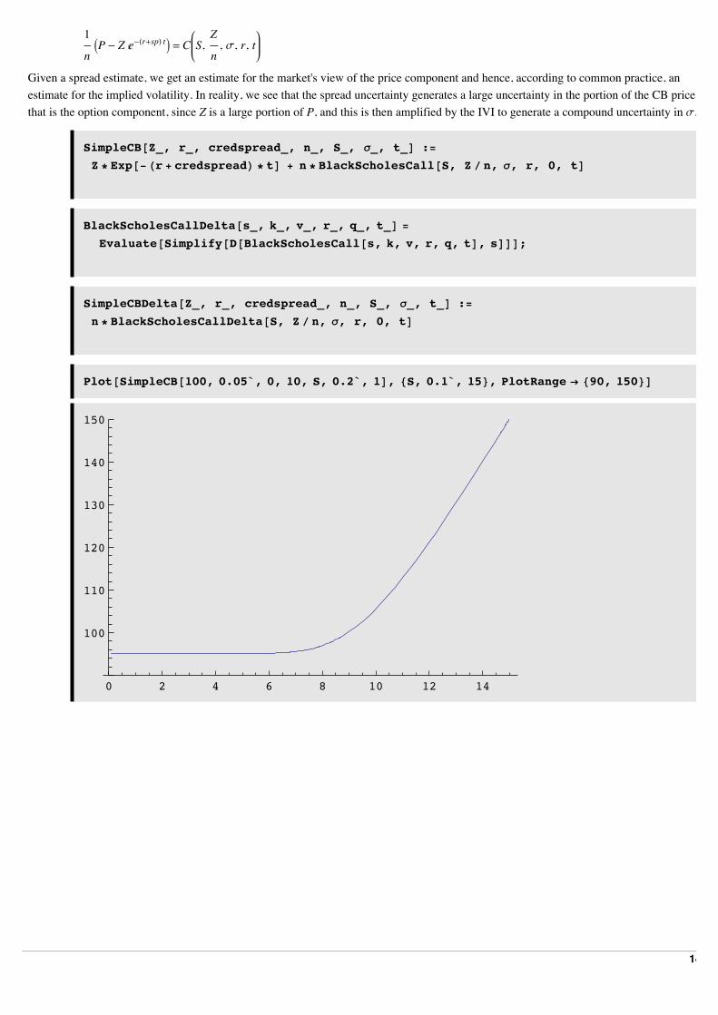
Given a spread estimate, we get an estimate for the market's view of the price component and hence, according to common practice, an estimate for the implied volatility. In reality, we see that the spread uncertainty generates a large uncertainty in the portion of the CB price that is the option component, since Z is a large portion of P, and this is then amplified by the IVI to generate a compound uncertainty in s.

SimpleCB@Z_, r_, credspread_, n_, S_, s_, t_D :=Z * Exp@-Hr + credspreadL * tD + n * BlackScholesCall@S, Z ê n, s, r, 0, tD

BlackScholesCallDelta@s_, k_, v_, r_, q_, t_D =

Evaluate@Simplify@D@BlackScholesCall@s, k, v, r, q, tD, sDDD;

SimpleCBDelta@Z_, r_, credspread_, n_, S_, s_, t_D :=n * BlackScholesCallDelta@S, Z ê n, s, r, 0, tD

Plot@SimpleCB@100, 0.05`, 0, 10, S, 0.2`, 1D, 8S, 0.1`, 15<, PlotRange Ø 890, 150<D

0 2 4 6 8 10 12 14

100

110

120

130

140

150

14

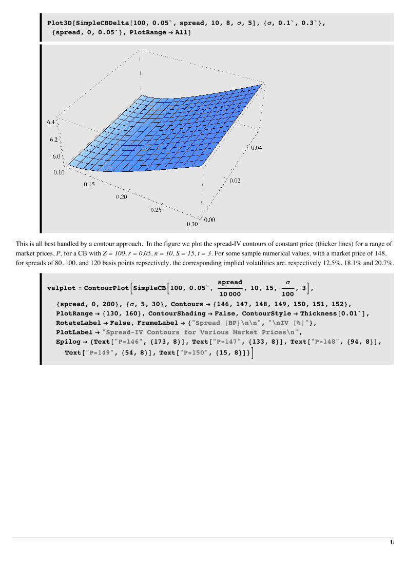
Plot3D@SimpleCBDelta@100, 0.05`, spread, 10, 8, s, 5D, 8s, 0.1`, 0.3`<,8spread, 0, 0.05`<, PlotRange Ø AllD

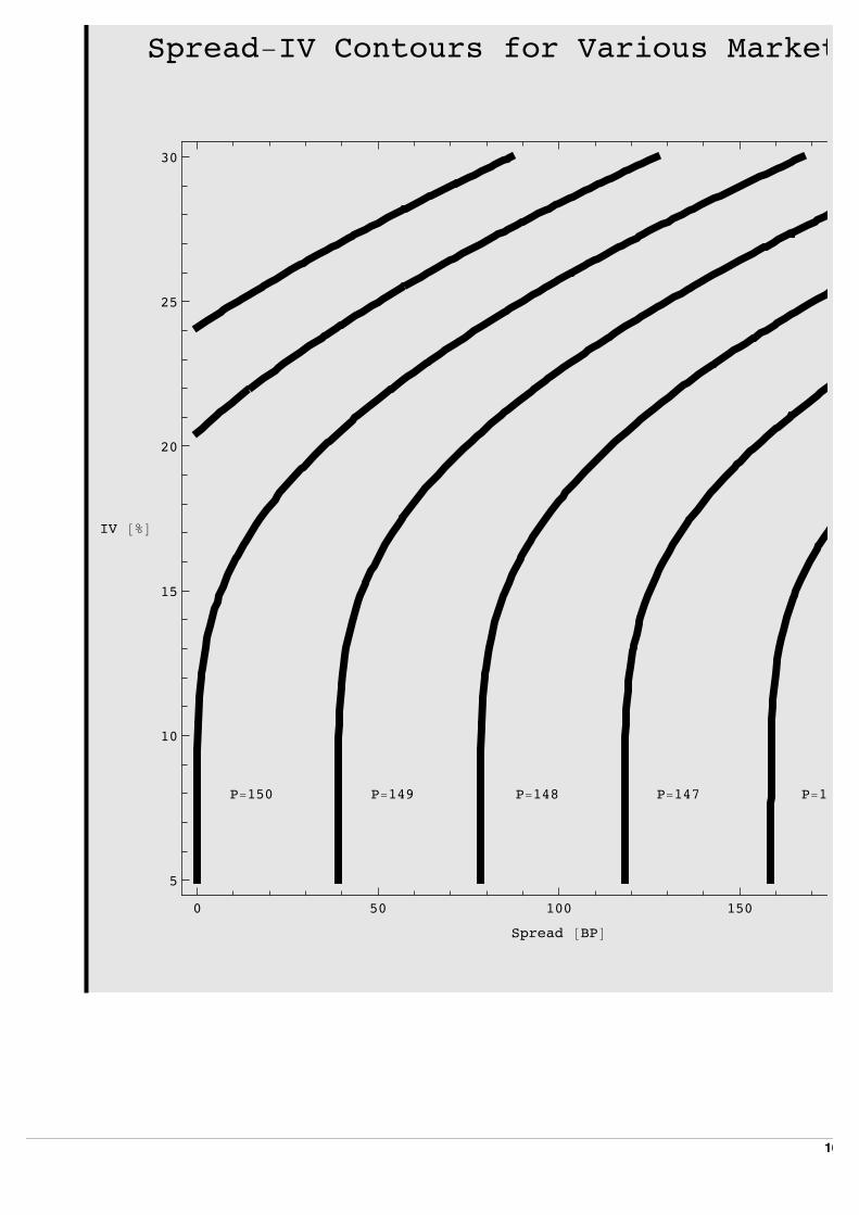
This is all best handled by a contour approach. In the figure we plot the spread-IV contours of constant price (thicker lines) for a range of market prices, P, for a CB with Z = 100, r = 0.05, n = 10, S = 15, t = 3. For some sample numerical values, with a market price of 148, for spreads of 80, 100, and 120 basis points repsectively, the corresponding implied volatilities are, respectively 12.5%, 18.1% and 20.7%.

valplot = ContourPlotBSimpleCBB100, 0.05`,spread

10 000, 10, 15,

s

100, 3F,

8spread, 0, 200<, 8s, 5, 30<, Contours Ø 8146, 147, 148, 149, 150, 151, 152<,PlotRange Ø 8130, 160<, ContourShading Ø False, ContourStyle Ø Thickness@0.01`D,RotateLabel Ø False, FrameLabel Ø 8"Spread @BPD\n\n", "\nIV @%D"<,PlotLabel Ø "Spread-IV Contours for Various Market Prices\n",Epilog Ø 8Text@"P=146", 8173, 8<D, Text@"P=147", 8133, 8<D, Text@"P=148", 894, 8<D,

Text@"P=149", 854, 8<D, Text@"P=150", 815, 8<D<F

15

0 50 100 150

5

10

15

20

25

30

Spread @BPD

IV @%D

Spread-IV Contours for Various Market Prices

P=146P=147P=148P=149P=150

16

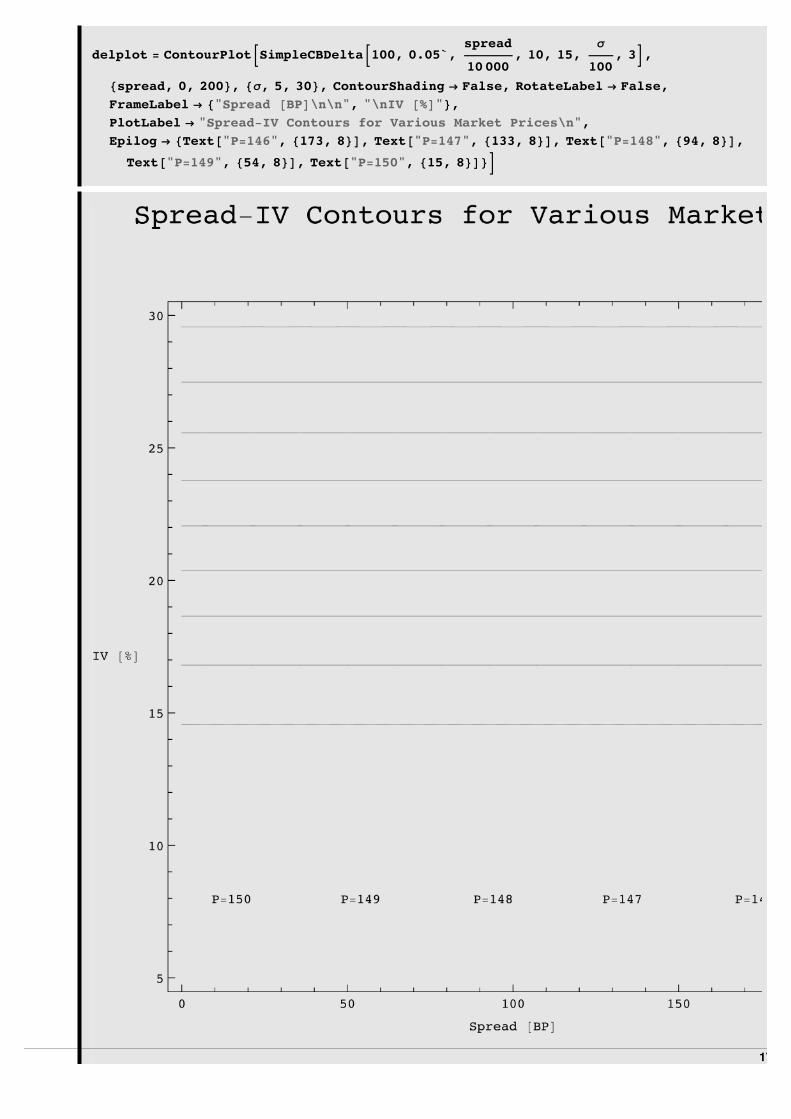
delplot = ContourPlotBSimpleCBDeltaB100, 0.05`,spread

10 000, 10, 15,

s

100, 3F,

8spread, 0, 200<, 8s, 5, 30<, ContourShading Ø False, RotateLabel Ø False,FrameLabel Ø 8"Spread @BPD\n\n", "\nIV @%D"<,PlotLabel Ø "Spread-IV Contours for Various Market Prices\n",Epilog Ø 8Text@"P=146", 8173, 8<D, Text@"P=147", 8133, 8<D, Text@"P=148", 894, 8<D,

Text@"P=149", 854, 8<D, Text@"P=150", 815, 8<D<F

17

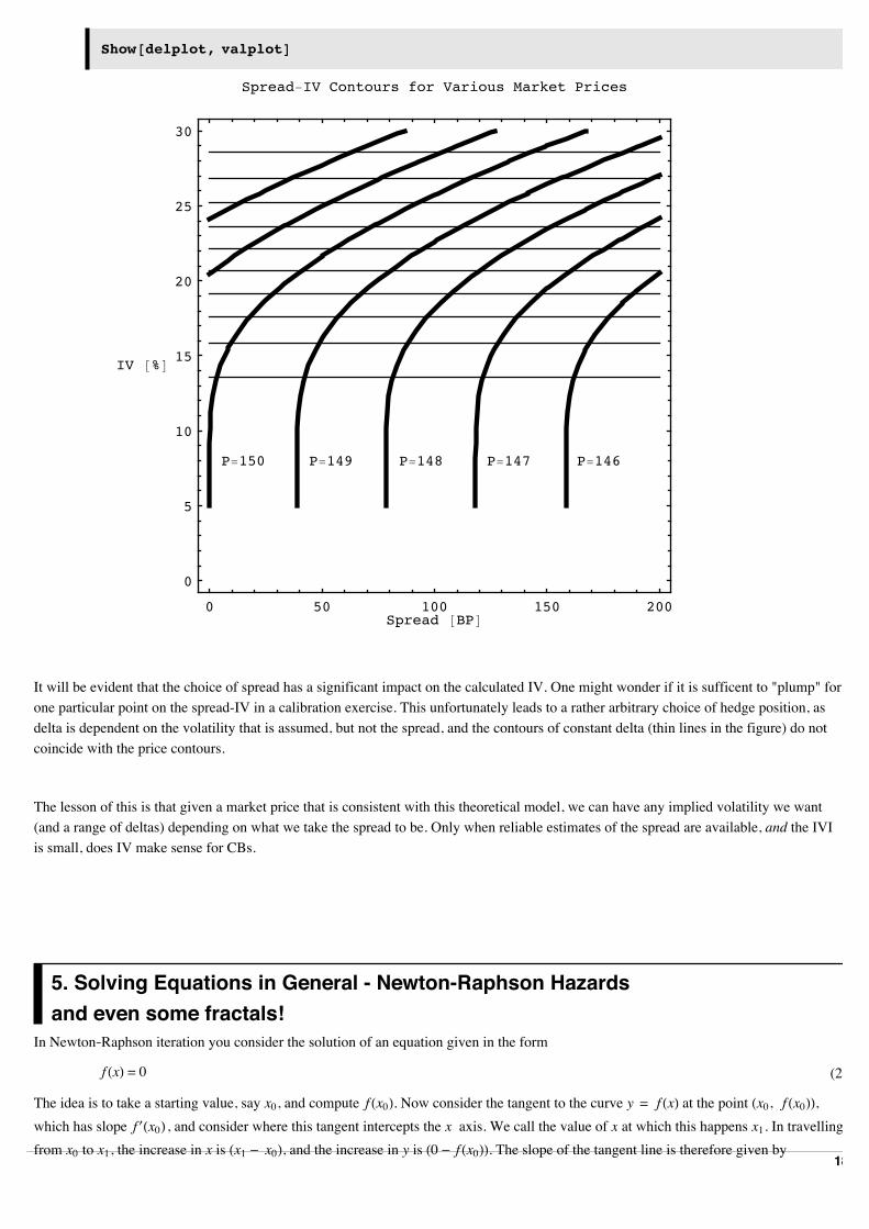
Show@delplot, valplotD

0 50 100 150 200Spread @BPD

0

5

10

15

20

25

30

IV @%D

Spread-IV Contours for Various Market Prices

P=146P=147P=148P=149P=150

It will be evident that the choice of spread has a significant impact on the calculated IV. One might wonder if it is sufficent to "plump" for one particular point on the spread-IV in a calibration exercise. This unfortunately leads to a rather arbitrary choice of hedge position, as delta is dependent on the volatility that is assumed, but not the spread, and the contours of constant delta (thin lines in the figure) do not coincide with the price contours.

The lesson of this is that given a market price that is consistent with this theoretical model, we can have any implied volatility we want (and a range of deltas) depending on what we take the spread to be. Only when reliable estimates of the spread are available, and the IVI is small, does IV make sense for CBs.

5. Solving Equations in General - Newton-Raphson Hazardsand even some fractals!

In Newton|Raphson iteration you consider the solution of an equation given in the form

(2)f HxL = 0

The idea is to take a starting value, say x0, and compute f Hx0L. Now consider the tangent to the curve y = f HxL at the point Hx0, f Hx0LL, which has slope f £Hx0L , and consider where this tangent intercepts the x axis. We call the value of x at which this happens x1. In travelling from x0 to x1, the increase in x is Hx1 - x0L, and the increase in y is H0 - f Hx0LL. The slope of the tangent line is therefore given by

18

(3)0 - f Hx0L

x1 - x0

and this must be equal to f £Hx0L. This gives us an equation governing x1:

(4)0 - f Hx0L

x1 - x0= f £Hx0L

which we can solve for x1, obtaining

(5)x1 = x0 -f Hx0L

f £Hx0L

This now defines a new iteration scheme, since we can just repeat this process, defining

(6)xn+1 = xn -f HxnL

f £HxnL

This defines the famous ‘Newton|Raphson’ iteration scheme.

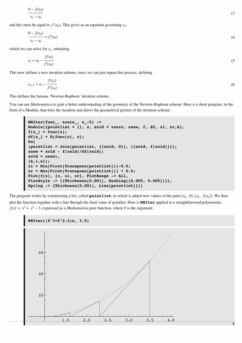
You can use Mathematica to gain a better understanding of the geometry of the Newton|Raphson scheme. Here is a short program, in the form of a Module, that does the iteration and draws the geometrical picture of the iteration scheme:

NRIter[func_, xzero_, n_:5] :=Module[{pointlist = {}, x, xold = xzero, xnew, f, df, xl, xr,k},f[x_] = func[x];df[x_] = D[func[x], x];Do[(pointlist = Join[pointlist, {{xold, 0}}, {{xold, f[xold]}}];xnew = xold - f[xold]/df[xold];xold = xnew),{k,1,n}];xl = Min[First[Transpose[pointlist]]]-0.5; xr = Max[First[Transpose[pointlist]]] + 0.5;Plot[f[x], {x, xl, xr}, PlotRange -> All,PlotStyle -> {{Thickness[0.001], Dashing[{0.005, 0.005}]}},Epilog -> {Thickness[0.001], Line[pointlist]}]]

The program works by constructing a list, called pointlist, to which is added new values of the pairs Hxn, 0L, Hxn, f HxnLL. We then plot the function together with a line through the final value of pointlist. Here is NRIter applied to a straightforward polynomial, f HxL = x3 + x2 - 3, expressed as a Mathematica pure function, where # is the argument:

NRIter[(#^3+#^2-3)&, 3.5]

1.5 2.0 2.5 3.0 3.5 4.0

20

40

60

As you can see, you do not have to change the function very much to obtain more complicated behaviour:

19

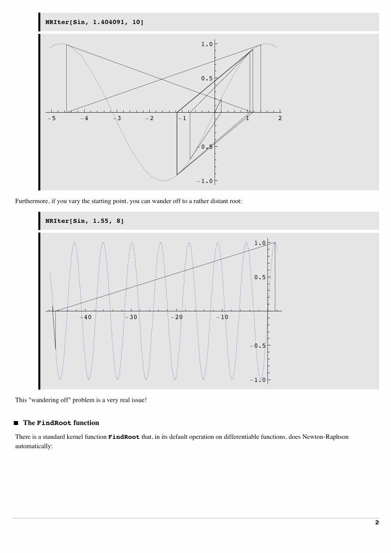
NRIter[Sin, 1.404091, 10]

-5 -4 -3 -2 -1 1 2

-1.0

-0.5

0.5

1.0

Furthermore, if you vary the starting point, you can wander off to a rather distant root:

NRIter[Sin, 1.55, 8]

-40 -30 -20 -10

-1.0

-0.5

0.5

1.0

This "wandering off" problem is a very real issue!

‡ The FindRoot function

There is a standard kernel function FindRoot that, in its default operation on differentiable functions, does Newton|Raphson automatically:

20

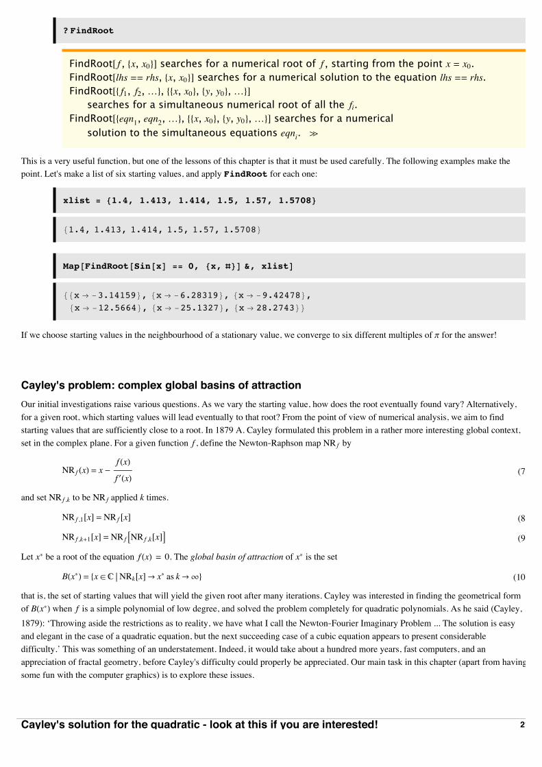
? FindRoot

FindRoot@ f , 8x, x0<D searches for a numerical root of f , starting from the point x = x0.FindRoot@lhs == rhs, 8x, x0<D searches for a numerical solution to the equation lhs == rhs.FindRoot@8 f1, f2,…<, 88x, x0<, 8y, y0<,…<D

searches for a simultaneous numerical root of all the fi.FindRoot@8eqn1, eqn2,…<, 88x, x0<, 8y, y0<,…<D searches for a numerical

solution to the simultaneous equations eqni.  à

This is a very useful function, but one of the lessons of this chapter is that it must be used carefully. The following examples make the point. Let's make a list of six starting values, and apply FindRoot for each one:

xlist = 81.4, 1.413, 1.414, 1.5, 1.57, 1.5708<

81.4, 1.413, 1.414, 1.5, 1.57, 1.5708<

Map@FindRoot@Sin@xD == 0, 8x, Ò<D &, xlistD

88x Ø -3.14159<, 8x Ø -6.28319<, 8x Ø -9.42478<,8x Ø -12.5664<, 8x Ø -25.1327<, 8x Ø 28.2743<<

If we choose starting values in the neighbourhood of a stationary value, we converge to six different multiples of p for the answer!

Cayley's problem: complex global basins of attractionOur initial investigations raise various questions. As we vary the starting value, how does the root eventually found vary? Alternatively, for a given root, which starting values will lead eventually to that root? From the point of view of numerical analysis, we aim to find starting values that are sufficiently close to a root. In 1879 A. Cayley formulated this problem in a rather more interesting global context, set in the complex plane. For a given function f , define the Newton|Raphson map NR f by

(7)NR f HxL = x -f HxL

f £HxL

and set NR f ,k to be NR f applied k times.

(8)NR f ,1@xD = NR f @xD

(9)NR f ,k+1@xD = NR f ANR f ,k@xDE

Let x* be a root of the equation f HxL = 0. The global basin of attraction of x* is the set

(10)BHx*L = 8x œ C NRk@xDØ x* as k ض<

that is, the set of starting values that will yield the given root after many iterations. Cayley was interested in finding the geometrical form of BHx*L when f is a simple polynomial of low degree, and solved the problem completely for quadratic polynomials. As he said (Cayley, 1879): ‘Throwing aside the restrictions as to reality, we have what I call the Newton|Fourier Imaginary Problem ... The solution is easy and elegant in the case of a quadratic equation, but the next succeeding case of a cubic equation appears to present considerable difficulty.’ This was something of an understatement. Indeed, it would take about a hundred more years, fast computers, and an appreciation of fractal geometry, before Cayley's difficulty could properly be appreciated. Our main task in this chapter (apart from having some fun with the computer graphics) is to explore these issues.

Cayley's solution for the quadratic - look at this if you are interested!Let's consider the equation arising from solving the quadratic equation

21

(11)f HzL = z2 - 1 = 0

The Newton|Raphson mapping for this case is easily seen to be

(12)NR f HzL =1

2z +

1

z

The solution for the basins of attraction of this problem will represent an early encounter for you with the type of mapping known as a Möbius map. These maps will reappear many times in different applications. Here its role is to make a transformation that makes it obvious what the basins of attraction are for the Newton-Raphson solution of a quadratic equation. The form of the mapping can be appreciated by noting that what we want to do is to transform the point z = 1 to the origin, and the point z = -1 to infinity. This can be achieved by setting

(13)w = MHzL =z - 1

z + 1

You can easily check that the corresponding inverse mapping is obtained by setting

(14)z = M-1HwL =1 + w

1 - w

What mapping does NRHzL induce in w-coordinates? This is the mapping

(15)w Ø NRèHwL = MINRIM-1HwLMM

Some algebra (it is left for you as an exercise) leads to the observation that

(16)NRèHwL = w2

If you work in w-coordinates, and iterate this mapping, it is obvious that wn Ø 0 if w0 < 1, and that wn ض if w0 > 1. So in these coordinates, the basins of attraction are the interior and exterior of the unit circle. Points on the unit circle just get mapped around on the unit circle, and the unit circle is the boundary between the two basins. Now you just have to interpret this in z-coordinates. Clearly, if wn Ø 0, then zn Ø 1, and if wn ض, then zn Ø-1, and what is required is an understanding of what the unit circle, in w-coordinates, is in z-coordinates. If you set

(17)w = ‰if

then it is a simple exercise to show that

(18)z = Â cotf

2

so that as f varies the whole of the imaginary axis is obtained. So in z-coordinates the boundary between the two basins is the imaginary axis. In other words, the basins are given by two (left and right) half-planes:

(19)BH1L = 8z œ C ReHzL > 0<

(20)BH-1L = 8z œ C ReHzL < 0<

In the case of a general quadratic mapping similar results apply | the plane is divided into two basins by the perpendicular bisector of the line joining the two roots.

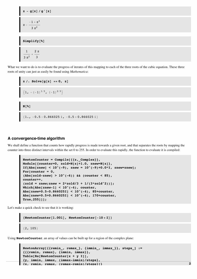
Basins of attraction for a simple cubicCayley's attempts to establish a similar result for cubics failed. A full appreciation of the reasons why is beyond the scope of this book, but you can get a good grip on why matters are more complicated by simulation using Mathematica. First, let's construct the Newton|Raphson mapping:

g[z_] := z^3 - 1

22

z - g@zD ê g'@zD

z --1 + z3

3 z2

Simplify@%D

1

3 z2+2 z

3

What we want to do is to evaluate the progress of iterates of this mapping to each of the three roots of the cubic equation. These three roots of unity can just as easily be found using Mathematica:

z ê. Solve@g@zD == 0, zD

91, -H-1L1ê3, H-1L2ê3=

N@%D

81., -0.5 - 0.866025 Â, -0.5 + 0.866025 Â<

A convergence-time algorithmWe shall define a function that counts how rapidly progress is made towards a given root, and that separates the roots by mapping the counter into three distinct intervals within the set 0 to 255. In order to evaluate this rapidly, the function to evaluate it is compiled:

NewtonCounter = Compile[{{z,_Complex}},Module[{counter=0, zold=N[z]+1.0, znew=N[z]},If[Abs[znew] < 10^(-9), znew = 10^(-9)+0.0*I, znew=znew];For[counter = 0,(Abs[zold-znew] > 10^(-6)) && (counter < 85), counter++,(zold = znew;znew = 2*zold/3 + 1/(3*zold^2))];Which[Abs[znew-1] < 10^(-4), counter,Abs[znew+0.5-0.866025I] < 10^(-4), 85+counter,Abs[znew+0.5+0.866025I] < 10^(-4), 170+counter,True,255]]];

Let's make a quick check to see that it is working:

8NewtonCounter@1.001D, NewtonCounter@-10 + ID<

82, 105<

Using NewtonCounter, an array of values can be built up for a region of the complex plane:

NewtonArray[{{remin_, remax_}, {immin_, immax_}}, steps_] :={{{remin, remax}, {immin, immax}},Table[Re[NewtonCounter[x + y I]],{y, immin, immax, (immax-immin)/steps},{x, remin, remax, (remax-remin)/steps}]}

Colouring schemes

23

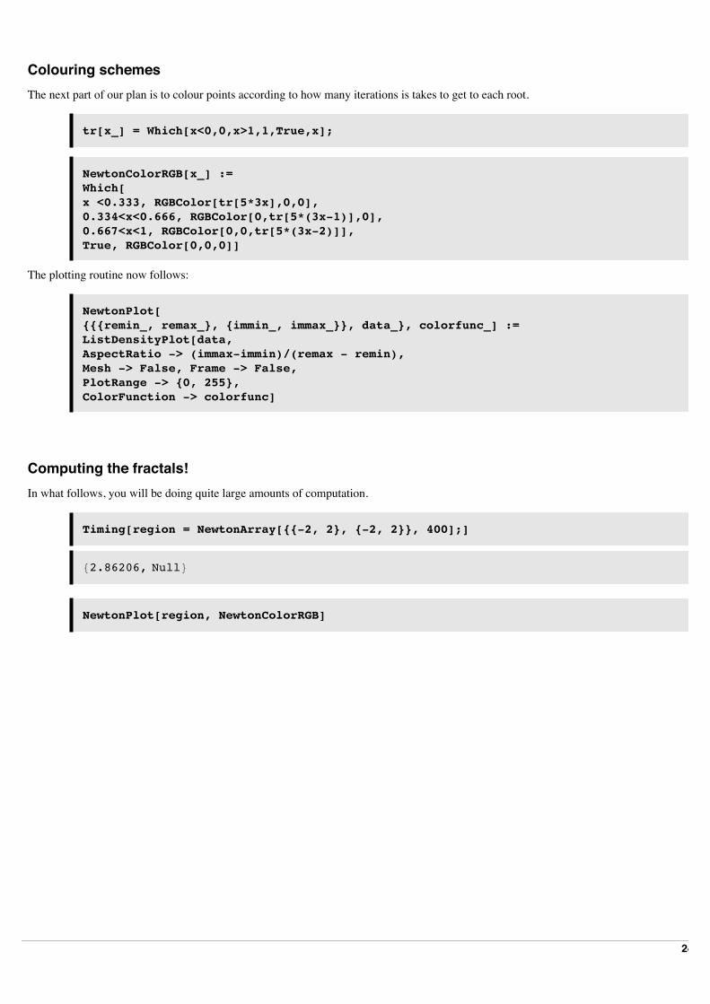
Colouring schemesThe next part of our plan is to colour points according to how many iterations is takes to get to each root.

tr[x_] = Which[x<0,0,x>1,1,True,x];

NewtonColorRGB[x_] :=Which[x <0.333, RGBColor[tr[5*3x],0,0], 0.334<x<0.666, RGBColor[0,tr[5*(3x-1)],0],0.667<x<1, RGBColor[0,0,tr[5*(3x-2)]], True, RGBColor[0,0,0]]

The plotting routine now follows:

NewtonPlot[{{{remin_, remax_}, {immin_, immax_}}, data_}, colorfunc_] :=ListDensityPlot[data,AspectRatio -> (immax-immin)/(remax - remin),Mesh -> False, Frame -> False,PlotRange -> {0, 255}, ColorFunction -> colorfunc]

Computing the fractals!In what follows, you will be doing quite large amounts of computation.

Timing[region = NewtonArray[{{-2, 2}, {-2, 2}}, 400];]

82.86206, Null<

NewtonPlot[region, NewtonColorRGB]

24

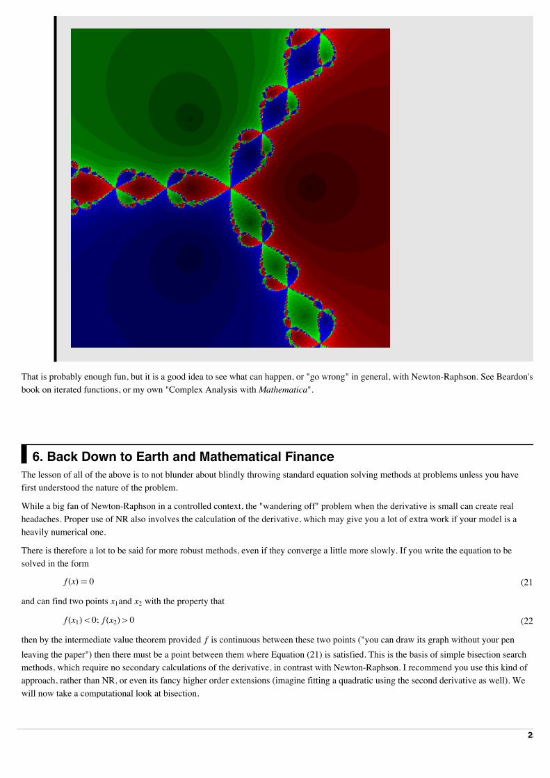
That is probably enough fun, but it is a good idea to see what can happen, or "go wrong" in general, with Newton-Raphson. See Beardon's book on iterated functions, or my own "Complex Analysis with Mathematica".

6. Back Down to Earth and Mathematical FinanceThe lesson of all of the above is to not blunder about blindly throwing standard equation solving methods at problems unless you have first understood the nature of the problem.

While a big fan of Newton-Raphson in a controlled context, the "wandering off" problem when the derivative is small can create real headaches. Proper use of NR also involves the calculation of the derivative, which may give you a lot of extra work if your model is a heavily numerical one.

There is therefore a lot to be said for more robust methods, even if they converge a little more slowly. If you write the equation to be solved in the form

(21)f HxL‡ 0

and can find two points x1and x2 with the property that

(22)f Hx1L < 0; f Hx2L > 0

then by the intermediate value theorem provided f is continuous between these two points ("you can draw its graph without your pen leaving the paper") then there must be a point between them where Equation (21) is satisfied. This is the basis of simple bisection search methods, which require no secondary calculations of the derivative, in contrast with Newton-Raphson. I recommend you use this kind of approach, rather than NR, or even its fancy higher order extensions (imagine fitting a quadratic using the second derivative as well). We will now take a computational look at bisection.

Acknowledgements

25

AcknowledgementsThe contour approach to the CB analysis was developed by Roger Wilson.

Nomura International plc

ReferencesShaw, W.T. 1998, Modelling Financial Derivatives with Mathematica, Cambridge University Press, 1998.

An overview of this work appeared in a series of articles in Financial Products - Financial Engineering News, Vol.2, Issues 5, 6, 9 (Aug, Sep, 1999).

On WS' web site:

http://www.mth.kcl.ac.uk/~shaww/web_page/papers/WebChronoPapers.htm

Shaw, W.T. and Lee, K.T.A., 2006, Copula Methods vs Canonical Multivariate Distributions | the multivariate Student T distribution with general degrees of freedom, November 2006 (submitted)

Shaw, W.T., 2006, Sampling Student’s T distribution | use of the inverse cumulative distribution function. Journal of Computational Finance, Vol 9 Issue 4, pp 37-73, Summer 2006

26